«M?

;$«,

AN EVALUATION OF THE APPROPRIATENESS OF THE

DEFENSE LOGISTICS AGENCY'S REQUIREMENTS MODEL

THESIS

Harry A. Berry, M.B.A. Captain, USAF

Edward E. Tatge, B.S. Captain, USAF

AFIT/GIM/LAL/95S-1

DEPARTMENT OF THE AIR FORCE

AIR UNIVERSITY

AIR FORCE INSTITUTE OF TECHNOLOGY

Wright-Patterson Air Force Base, Ohio

OTIO QUALITY INSPECTED 0

AHT/GIM/LAL/95S-1

AN EVALUATION OF THE APPROPRIATENESS OF THE

DEFENSE LOGISTICS AGENCY'S REQUIREMENTS MODEL

THESIS

Harry A. Berry, M.B.A. Edward E. Tatge, B.S. Captain, USAF Captain, USAF

AFIT/GIM/LAL/95S-1

19951102101 Approved for public release; distribution unlimited

The views expressed in this thesis are those of the authors and do not reflect the official policy or position of the

Department of Defense or the U.S. Government.

Accession for *"<3WW

ITIS QRAJbl W DTIC TAB Q Unanoou»ced Q Justification —

By Distribution/-

Availability Coiot

Blat Avail and/oj?

Special

AFIT/GIM/LAL/95S-1

AN EVALUATION OF THE APPROPRIATENESS OF THE

DEFENSE LOGISTICS AGENCY'S REQUIREMENTS MODEL

THESIS

Presented to the Faculty of the Graduate School of Logistics

and Acquisition Management of the Air Force Institute of Technology

Air University

In Partial Fulfillment of the

Requirements for the Degree of

Master of Science in Logistics Management

Harry A. Berry, M.B.A. Edward E. Tatge, B.S.

Captain, USAF Captain, USAF

September 1995

Acknowledgments

The authors wish to express their sincere appreciation to Dr. Rajesh Srivastava,

our thesis advisor, and Major Terrance L. Pohlen, our thesis reader, for their guidance and

support during this research. In addition, the authors would like to thank Dr. V. Dan

Guide and Major Mark E. Kraus for their assistance in making our simulation models

work correctly.

Thanks is also offered to Mr. Nandakumar M. Balwally and Mr. Robert Bilikam,

Operations Research Analysis and Projects Division, Defense Logistics Agency, Defense

Electronics Supply Center, for their insight, research assistance, and data collection skills.

Finally, but most importantly, thanks are given to our wives, Sandy and Sarah, for

the deprivations they have endured for the past fifteen months and for their understanding,

patience, and support during this period.

Harry A. Berry Edward E Tatge

Table of Contents

Page

Acknowledgments ü

List of Figures v

List of Tables vi

Abstract viii

I. Background and Problem Presentation 1-1

Introduction 1-1

The Requirements Model 1-2

Research Objectives 1-6

Methodology 1-7

Scope and Limitations 1-7

Organization of Thesis 1-8

n. Literature Review 2-1

Inventory 2-1

Purpose of Inventory 2-3

Inventory Costs 2-4

The Defense Logistics Agency 2-9

The DLA Model 2-11

Lumpy Demand 2-16

Related Studies 2-18

HI. Methodology 3-1

Conducting An Experiment 3-1

Selecting Relevant Variables 3-2

Factors and Levels of Treatment 3-4

Experimental Environment 3-8

Experimental Design 3-9

in

Page

Select and Assign the Subjects 3-16

Testing Data 3-17

Analyze the Data 3-17

IV. Data Analysis 4-1

Proposed Statistical Analysis 4-1

Output Data Analysis 4-2

V. Conclusions, Implications and Recommendations 5-1

Conclusions 5-1

Implications 5-3

Recommendations for Future Research 5-4

Appendix A. Sample Data A-l

Appendix B. Graph of Sample Demand Pattern A-3

Appendix C. Model Description and Code A-4

Appendix D. Transient Period Determination A-21

Appendix E. Sample Size Determination A-23

Appendix F. Test for Normality A-25

Appendix G. Test Results A-27

Appendix H. Silver-Meal Model Description A-32

Appendix I. Lumpy Demand Application A-33

Appendix J. Graph of Lead Time Pattern A-35

References REF-1

Berry Vita V-l

TatgeVita • V-2

IV

List of Figures

Figure ^a§e

1-1. Assumptions met (Tersine, 1994: 93) 1-3

1-2. Assumptions not met (Tersine, 1994: 207)... 1-4

2-1. Cost Curve (Tersine: 94) 2-7

List of Tables

Table Page

1-1. Assumptions of Wilson's Classic Economic Order Quantity Model 1-2

2-1. DLA Supply Centers 2-10

2-2. SMCC Categories • 2-14

3-1. Long's Experimental Factors and Levels 3-6

3-2. Steps For Successful Simulation 3-10

3-3. Comparison of Models 3-12

3-4. Expected Analysis of Results 3-18

4-1. Average On-Hand Inventory Values 4-3

4-2. Test of Hypothesis C&C vs. Lumpy 4-4

4-3. Test of Hypothesis, Lumpy vs. Normal 4-5

4-4. Test of Hypothesis, Lumpy vs. Silver-Meal 4-6

4-5. Total Variable Cost Values 4-7

4-6. Test of Hypothesis C&C vs. Lumpy ..........4-8

4-7. Test of Hypothesis, Lumpy vs. Normal .....4-9

4-8. Test of Hypothesis, Lumpy vs. Silver-Meal 4-10

A-l. Sample Data • A-l

C-l. Global Definitions A-19

C-2. Entity Attributes A-20

C-3. Files • A-20

C-4. Resources • A-20

E-l. Required Runs A-24

VI

Page

F-l. Test for Normality A-25

G-l. Confidence Intervals A-31

1-1. Demand Patterns A-33

1-2. Silver and Meal's Heuristic Results A-34

vu

AHT/GIM/LAL/95S-1

Abstract

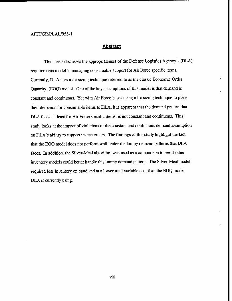
This thesis discusses the appropriateness of the Defense Logistics Agency's (DLA)

requirements model in managing consumable support for Air Force specific items.

Currently, DLA uses a lot sizing technique referred to as the classic Economic Order

Quantity, (EOQ) model. One of the key assumptions of this model is that demand is

constant and continuous. Yet with Air Force bases using a lot sizing technique to place

their demands for consumable items to DLA, it is apparent that the demand pattern that

DLA faces, at least for Air Force specific items, is not constant and continuous. This

study looks at the impact of violations of the constant and continuous demand assumption

on DLA's ability to support its customers. The findings of this study highlight the fact

that the EOQ model does not perform well under the lumpy demand patterns that DLA

faces. In addition, the Silver-Meal algorithm was used as a comparison to see if other

inventory models could better handle this lumpy demand pattern. The Silver-Meal model

required less inventory on hand and at a lower total variable cost than the EOQ model

DLA is currently using.

vin

AN EVALUATION OF THE APPROPRIATENESS OF THE DEFENSE

LOGISTICS AGENCY REQUIREMENTS MODEL

I. Background and Problem Presentation

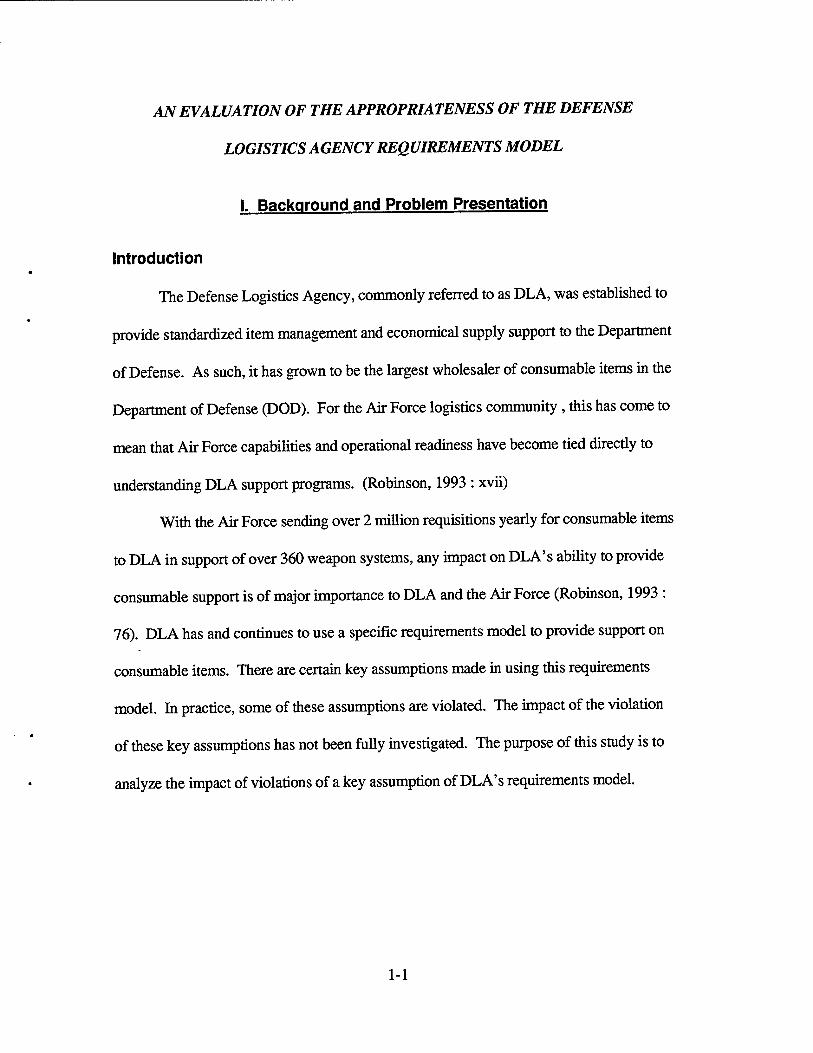
Introduction

The Defense Logistics Agency, commonly referred to as DLA, was established to

provide standardized item management and economical supply support to the Department

of Defense. As such, it has grown to be the largest wholesaler of consumable items in the

Department of Defense (DOD). For the Air Force logistics community , this has come to

mean that Air Force capabilities and operational readiness have become tied direcüy to

understanding DLA support programs. (Robinson, 1993 : xvii)

With the Air Force sending over 2 million requisitions yearly for consumable items

to DLA in support of over 360 weapon systems, any impact on DLA's ability to provide

consumable support is of major importance to DLA and the Air Force (Robinson, 1993 :

76). DLA has and continues to use a specific requirements model to provide support on

consumable items. There are certain key assumptions made in using this requirements

model. In practice, some of these assumptions are violated. The impact of the violation

of these key assumptions has not been fully investigated. The purpose of this study is to

analyze the impact of violations of a key assumption of DLA's requirements model.

1-1

The Requirements Model

In an interview with Captain William Long on June 21,1994, Mr. N. Balwally, a

member of the Operations Research Analysis and Projects Division, Defense Electronics

Supply Center, stated that the requirements model currently used by DLA is a hybrid of

Wilson's Economic Order Quantity (EOQ) model with an additional variable safety stock

(Long, 1994:2). Both the Wilson and the DLA EOQ models attempt to minimize total

variable costs by finding the point where holding costs and ordering costs balance.

In order to use these models, certain assumptions must be made. These

assumptions, as they apply to both models, are listed in Table 1.

Table 1-1. Assumptions of Wilson's Classic Economic Order Quantity Model

1. The demand rate is known, constant, and continuous 2. The lead time is known and constant 3. The entire lot size is added to inventory at the same time 4. No stockouts are permitted; since demand and lead time are known, stockouts can be

avoided 5. The cost structure is fixed; order/setup costs are the same regardless of the lot size,

holding cost is a linear function based on average inventory, and unit purchase cost is constant

6. There is sufficient space, capacity, and capital to procure the desired quantity 7. The item is a single product; it does not interact with any other inventory items (there

are know joint orders) ___ (Tersine, 1994: 95)

These assumptions are required to develop the model, but are not realistic in

normal business operations. "In reality, we find few cases where a deterministic EOQ

model can be used because we cannot satisfy all of the assumptions of the deterministic

model" (Hood, 1987:20). Although the hybrid models used by DLA and other companies

have been built to adjust to the dynamic environment of the real world, these models still

1-2

rely on the general assumptions listed in Table 1. This leads to the issue of what effect

does violations of the assumptions have on the model's ability to minimize overall variable

cost and inventory levels.

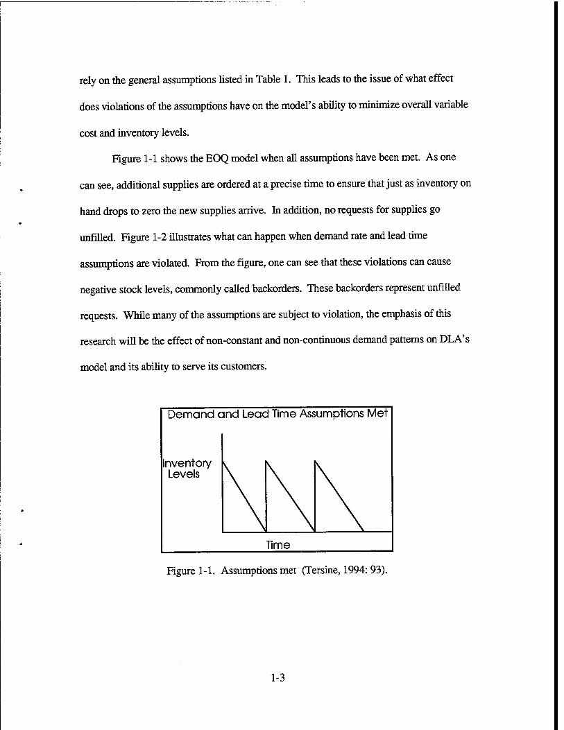
Figure 1-1 shows the EOQ model when all assumptions have been met. As one

can see, additional supplies are ordered at a precise time to ensure that just as inventory on

hand drops to zero the new supplies arrive. In addition, no requests for supplies go

unfilled. Figure 1-2 illustrates what can happen when demand rate and lead time

assumptions are violated. From the figure, one can see that these violations can cause

negative stock levels, commonly called backorders. These backorders represent unfilled

requests. While many of the assumptions are subject to violation, the emphasis of this

research will be the effect of non-constant and non-continuous demand patterns on DLA's

model and its ability to serve its customers.

Figure 1-1. Assumptions met (Tersine, 1994:93).

1-3

Demand and Lead Time Assumptions are Violatec

Inventory Levels

Time

Figure 1-2. Assumptions not met (Tersine, 1994: 207).

WJ

is

Given the somewhat unrealistic expectations of the EOQ model, one might wonder

hy anyone would use this model in practice. One of the key features of the EOQ model

its robustness. By this it is meant that the model can handle errors in the input variables,

holding cost, ordering cost, and demand rate, without significant changes in the total

variable cost (TVC) or the economic ordering quantity. According to Prichard and Eagle,

"Not only is the error in the TVC relatively insensitive to errors in individual parameters,

but it is affected only by the ratio of input error ratios, which may be less than the

individual error ratios" (Prichard and Eagle, 1965: 87-89).

The consumable requisitioning system for DLA and its customers is a multi-

echelon system. From an Air Force perspective, the first echelon is the base or retail level

which represents DLA's customers. DLA represents the second level, providing

consumable items to the bases. The third level is composed of DLA's vendors supplying

consumable items to DLA (Long, 1994 : 5).

1-4

From base level, consumable item demand is not constant or continuous. "Air

Force demand patterns tend to be lumpy and erratic" (Blazer, 1986 :1). At base level,

each base operates under an EOQ type model that emphasizes economic lot ordering to

balance ordering and holding costs (Hood, 1987 :22). Customer demands at base level,

regardless of the demand pattern, are consolidated into EOQ lot sizes and then sent to

DLA. This use of the EOQ model at the first level ensures that demands placed against

DLA are not constant or continuous, but lumpy from the lot size orders. This causes

DLA to face a demand pattern similar Figure 1-2 while their EOQ model assumes that

demands are like Figure 1-1. This disconnect can lead to stockouts or unnecessary stock

being carried by DLA depending on the type of lumpy demand pattern.

It is the effect of this lumpy demand placed against DLA's requirements model that

is the subject of this study. A significant negative impact on the model would ultimately

degrade customer support and call into question the appropriateness of the model under

these conditions. A prior thesis attempted to analyze this impact of demand rate and lead

time assumption violations on DLA's model. Unfortunately, the study, while providing a

practical observation that lumpy demand appears to effect the model, was unable to

establish any statistical significance because of problems with data manipulation (Long,

1994:69).

1-5

Research Objectives

The purpose of this research is to analyze the impact of demand rate assumption

violations on DLA's requirements model to support Air Force consumable demands. The

specific objectives are:

1. Evaluate and change, if necessary, the performance measures of total variable

cost and inventory levels at DLA as established in the prior thesis performed by Captains

Long and Engberson.

2. Gather and adjust data collected from the Defense Electronics Supply Center

(DESC) to provide a database to evaluate the effect of lumpy demand on the model.

3. Perform a simulation of DLA's model using the database to determine the

impact of lumpy demand on the model.

4. Statistically, determine if violations of the constant and continuous demand

assumption have any impact on DLA's requirements model in terms of total cost and

average inventory on hand.

5. Based on the first four steps, determine if DLA's model is the best model

available under "lumpy" demand conditions. The model will be evaluated in terms of total

cost and average inventory on hand.

In order to achieve the stated research objectives, specific research questions have

been established. These are:

1. How does lumpy demand affect the total variable cost portion of DLA's

requirements model?

1-6

2. How does lumpy demand affect DLA's requirements model with regard to

inventory levels maintained at DLA?

3. Can a different approach provide improvement over the existing DLA

model?

Answers to these questions will provide a picture of the total impact of lumpy

demand on DLA's model, customer support, and ultimately, the appropriateness of the

model under these conditions.

Methodology

The primary tool used in this research will be simulation. A model will be created

that replicates the primary functions of DLA's requirements model. The simulation model

will be manipulated using constant and continuous demand patterns to establish baselines

for variable cost and inventory levels. The second run of the model will be with the real

world requirements data collected from DESC, which is lumpy in nature, and a

comparison of the variable cost and inventory levels generated from each run will be

made. Statistical analysis will be used to quantify the significance of the differences in the

runs and ultimately establish whether the current DLA requirements model is appropriate

for the non-constant demands DLA faces.

Scope and Limitations

The scope of this research is on the impact of lumpy demand for consumable items

from Air Force bases placed against DLA's requirements model. The analysis will

1-7

concentrate on the effect over time of this lumpy demand. Therefore, data from DLA on

past Air Force demand patterns will be used to evaluate the effect of this lumpy demand.

In regard to this data, there are limiting factors. Because of budgetary and time

constraints, the data was collected from DESC as a representative sampling of DLA's

overall consumable national stock numbers. In addition, the data was collected by DESC

analysts. It is their belief that this data sampling is representative of the demand pattern

that the Air Force places on DLA.

Organization of Thesis

Chapter I has introduced the idea of lumpy demand and its effect on the Standard

EOQ model. In addition, the chapter established that DLA, which uses a hybrid of the

standard EOQ model, theoretically faces lumpy demand patterns. The impact of this

lumpy demand on DLA's model and its ability to support consumable requirements is the

emphasis of the remainder of this thesis.

Chapter II will focus on inventory theory and the theoretical effects of "lumpy"

demand on the EOQ model. In addition, Air Force consumable management philosophy

and prior Air Force studies on demand patterns will be discussed. Finally, the chapter will

describe DLA's requirements model in greater detail and compare it to the classical EOQ

model.

In Chapter IE, the methodology of the research will be discussed. The use of

simulation to answer the research questions posed in Chapter I will be justified. In

addition, the simulation model used to replicate DLA's requirements model will be

1-8

presented. Applicable variables , factors and levels of treatments, and simulation steps

taken will also be discussed. Finally, the proposed data analysis methodology will be

presented.

Chapter IV presents the data output from the simulation model, the analysis of the

data, and the results of the tests conducted on the data. Hypotheses about the data will be

rejected or not rejected based on the output data. This discussion will lay the foundation

for the conclusions and recommendations in Chapter V.

Chapter V will present the conclusions from the data provided in Chapter IV. The

adequacy of DLA's requirements model will be determined and based on this

determination, recommendations about the model as well as future research considerations

will be provided.

1-9

II. Literature Review

In order to understand the relationship between lumpy demand and DLA's

requirements model, it is important to first understand the concepts of inventory and the

EOQ model. The purpose of this chapter is to provide a basic understanding of these

concepts and then apply them directly to the issue of lumpy demand and the DLA

requirements model. The chapter begins with a review of inventory, to include the

definition of inventory, reasons for holding inventory, and the costs associated with

holding inventory. Next, the classic EOQ model will be analyzed and its basic

assumptions will be discussed.

Using these concepts, the review will then focus on DLA and the requirements

model. A brief review of DLA's mission and role will be provided and then a breakdown

of the requirements model will follow. After discussing DLA and its requirements model,

the review will focus on defining lumpy demand and examining the environment that DLA

operates within. Relevant research in this area will then be presented and discussed in

relation to DLA and its requirements model and operating environment

Inventory

The American Production and Inventory Control Society (APICS) define

inventory as "those stocks or items used to support production, supporting activities, and

customer service." (APICS, 1992: 23) Inventory is further categorized based on its utility

or purpose and divided into the following categories, "working stock, safety stock,

2-1

anticipation stock, pipeline stock, decoupling stock and psychic stock" (Tersine, 1994:7).

A closer look at each of these categories is required to fully understand why inventory is

acquired and maintained.

Working stock, also referred to as cycle stock or lot size stock, is inventory that is

purchased and held in anticipation of a need. Lot sizes allow purchasing to achieve

quantity discounts, as well as to minimize holding and ordering costs. These items are

commonly referred to as supplies or raw materials (Tersine, 1994:7-8).

Safety stock "is inventory held in reserve to protect against uncertainties of supply

and demand" (Tersine, 1994: 8). Safety stock also protects against stockouts during the

replenishment cycle or lead time, which is "the delay between placing an order for

materials and receiving the materials" (Knowles, 1989:724). Other factors influencing the

amount of safety stock are, the number of backorders allowed during one order cycle, the

cost to hold versus the cost to back order, or financial limitations within the organization.

Anticipation stock is "inventory built up to cope with peak seasonal demand,

erratic requirements, or deficiencies in production capacity" (Tersine, 1994: 8). These are

foreseen requirements that would typically exceed current stock levels and could be

negotiated for and purchased prior to the requirement.

Pipeline stock is inventory in transit that is ordered at a predetermined time

permitting continuation of the operation during lead time. The APICS definition of

pipeline stock is "inventory to fill the transportation network and distribution system

including the flow through intermediate stocking points" (APICS, 1992: 35).

2-2

Furthermore, "the flow time through the pipeline has a major effect on the amount of

inventory required in the pipeline" (APICS, 1992: 35).

Decoupling stock is inventory held to allow multiple production or manufacturing

operations to operate independently. Psychic stock refers to the items on display in retail

stores. Neither decoupling stock nor psychic stock have a significant role in the

environment DLA operates in, although decoupling stock stock is used in Air Force depot

level repair.

Purpose of Inventory

"Inventories are kept so that products are available when they are needed or

available for sale when customers want to buy them" (Knowles, 1989:722). Not for

profit organizations, like the Air Force, would not typically purchase inventory for resale

at a profit, but rather to have assets available when organizations and individuals request

it. The functional factors of inventory, time, discontinuity, uncertainty, and economy,

further stratify the need or purpose of inventory (Tersine, 1994: 6).

The time factor involves "the long process of production and distribution required

before goods reach the final consumer" (Tersine, 1994: 6). Here inventory is held to

cover the time necessary to develop and bring the product to the point of sale. Time

factor examples include the time to prepare and execute the purchase schedule, the actual

production time of the asset, and the transit time from vendor to customer.

Inventory held for the discontinuity factor absorbs the differences in vendor

production capacity and customer demand, thus allowing an uninterrupted inventory flow.

The uncertainty factor concerns unforeseen events that modify the original plans of the

2-3

organization such as errors in demand estimates, variable production yields, and shipping

delays. The economy factor includes efforts to achieve economies of scale and to take

advantage of cost-reducing alternatives (Tersine, 1994:7).

Inventory Costs

Historically inventory only represented a small amount of an organizations' total

investment. "It was better (and cheaper) to have the material than not to have it"

(Harding, 1990: 255). However, "as manufacturers became more efficient, more

automated; labor costs declined and material cost grew" (Harding, 1990: 255). Now

"purchased materials account for 60-70% of the cost to manufacture on a national

average" (Harding, 1990: 255). This means that overall inventory costs have increased

dramatically and therefore necessitate effective management control.

In order to better manage and control inventory, materiel managers must know the

specific costs incurred with inventory. In fact there are four primary costs associated with

inventory: purchase cost, order/setup cost, holding cost, and stockout cost. "The

purchase cost of an item is the unit purchase price if it is obtained from an external source,

or the unit production cost if it is produced internally" (Tersine, 1994: 13). Order and

setup costs include any cost associated with placing an order, mostly administrative time,

or physically reconfiguring a production operation or processes. Order and setup costs

are "usually assumed to vary directly with the number of order or setups placed and not at

all with the size of the order" (Tersine, 1994:14).

2-4

Holding costs, or carrying costs, are comprised of the costs associated with

purchasing and maintaining inventory. Many costs are considered in holding inventories

and typically include but are not limited to, cost of capital, obsolescence, shrinkage, taxes,

and manpower. Cost of capital or opportunity cost reflect the lost profit if the

organization had invested the money in the next best alternative to inventory.

Obsolescence is the risk incurred that inventory will lose value while being held.

Shrinkage indicates the amount of inventory lost to damage, pilferage or misconduct.

Some states consider inventory taxable property subject to annual collection. During the

time inventory is in storage, there is a cost associated with the manpower or material

handling equipment used to manage it. All of these costs vary directly with the amount of

inventory held (Tersine, 1994:14).

The stockout cost is "the economic consequence of an external or an internal

shortage" (Tersine, 1994: 14). In the retail market, no revenue is gained when goods are

unavailable for purchase. Military organizations do not necessarily incur revenue losses

due to stock outs but do incur additional expenses for back ordering or expediting,

shipping, and processing of assets not available in stock, loss of productive time in

maintenance, and aircraft downtime.

Managing inventory expenses is one of the primary functions of an inventory

manager. As organizations become increasingly concerned with financial efficiency, the

costs associated with inventory become increasingly critical.

"The aim of inventory control is to maintain inventories at such a level that the goals and objectives of the organization are achieved.

2-5

Poor control of inventory can create a negative cash flow, tie up large amounts of capital, limit the expansion of an organization through lack of capital, and reduce the return on investment by broadening the investment base." (Tersine, 1994:20)

To manage the inventory costs appropriately, the total annual costs for the

inventory must be calculated, which is the sum of the purchase cost, order cost, and

holding cost. The formula for total annual cost is:

TC(Q)=PR + ^-+^- (1) Q 2

where

R = annual demand in units,

P = purchase cost of an item,

C = ordering cost per order,

H = PF = holding cost per unit this year,

Q = lot size or order quantity in units,

F = annual holding cost as a fraction of unit cost,

TC(Q) = total annual costs for the inventory. (Tersine: 92)

There is an optimum level of investment in inventory where having too much can

impair finances just as much as having too little; too much inventory may result in

unnecessary holding costs, and too little inventory can result in disrupted operations

(Tersine, 1994: 21). Therefore it is imperative to minimize total costs which occurs when

2-6

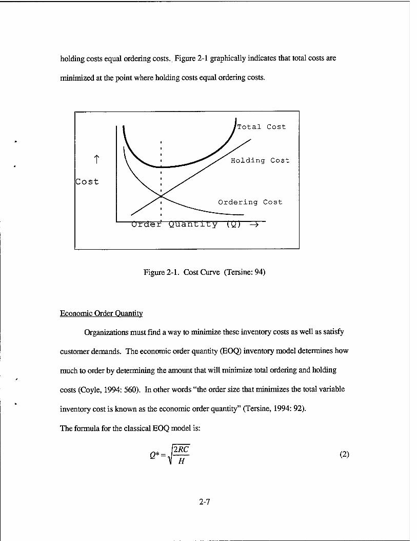
holding costs equal ordering costs. Figure 2-1 graphically indicates that total costs are

minimized at the point where holding costs equal ordering costs.

t

Cost

al Cost

ing Cost

ng Cost

urdef yuan-city CO") =T

Figure 2-1. Cost Curve (Tersine: 94)

Economic Order Quantity

Organizations must find a way to minimize these inventory costs as well as satisfy

customer demands. The economic order quantity (EOQ) inventory model determines how

much to order by determining the amount that will minimize total ordering and holding

costs (Coyle, 1994: 560). In other words "the order size that minimizes the total variable

inventory cost is known as the economic order quantity" (Tersine, 1994: 92).

The formula for the classical EOQ model is:

Q -i 2RC

H (2)

2-7

C = Cost to order

H = Holding cost

and,

H = PF

P = Price

F = Holding cost factor.

As stated in chapter I, the classical EOQ model is based on several key

assumptions. Based on these assumptions, Tersine highlights how the EOQ model reacts

to varying costs and unit prices.

"The EOQ results in an item with a high unit cost being ordered frequently in small quantities (the saving in inventory investment pays for the extra orders); an item with a low unit cost is ordered in large quantities (the inventory investment is small and the repeated expense of orders can be avoided). If the order cost is zero, orders are placed to satisfy each demand as it occurs, which results in no holding cost. If the holding cost H is zero, an order (only one) is placed for an amount that will satisfy the lifetime demand for the item." (Tersine: 94)

The EOQ model serves as the basis for DLA's requirements model, as will be shown in

the following section.

2-8

The EOQ model serves as the basis for DLA's requirements model, as will be shown in

the following section.

The Defense Logistics Agency

In August 1961, Secretary Robert S. MacNamara established the Defense Supply

Agency as an attempt to capitalize on the benefits of centralized logistical support for

common DOD items, while still providing the responsiveness that the Services had come

to rely on from their internal supply systems. At first, the Services were skeptical of the

ability of DS A to provide the specific support they required. There was a belief that each

Services individual needs would be overcome by the requirement to support a large

customer base as a whole. Over time, this belief was replaced by a growing dependence

on DSA for logistical support. DSA had quickly proven its ability to save the DOD

operating funds. In its first year of existence, DSA saved the DOD over $31 million while

providing better support than the inter-service systems it replaced. During the following

years, its role and mission expanded until the name, Defense Supply Agency, no longer

reflected the scope of its responsibilities. In 1977, the DSA became the Defense Logistics

Agency to reflect its growth from a supply manager to an agency handling the complete

logistical functions for numerous commodities (Robinson, 1994: 5).

Today, DLA's responsibilities can best be summed up by its mission statement. Its

primary mission is:

2-9

To function as an integral element of the DOD logistics system and to provide effective an efficient logistics support to DOD components as well as federal agencies, foreign governments, or international organizations as assigned in peace or war. Our vision at DLA is to continually improve the combat readiness of America's fighting forces by providing soldiers, sailors, airmen, and marines the best value in services when and where needed. (DLA, 1991:2-1)

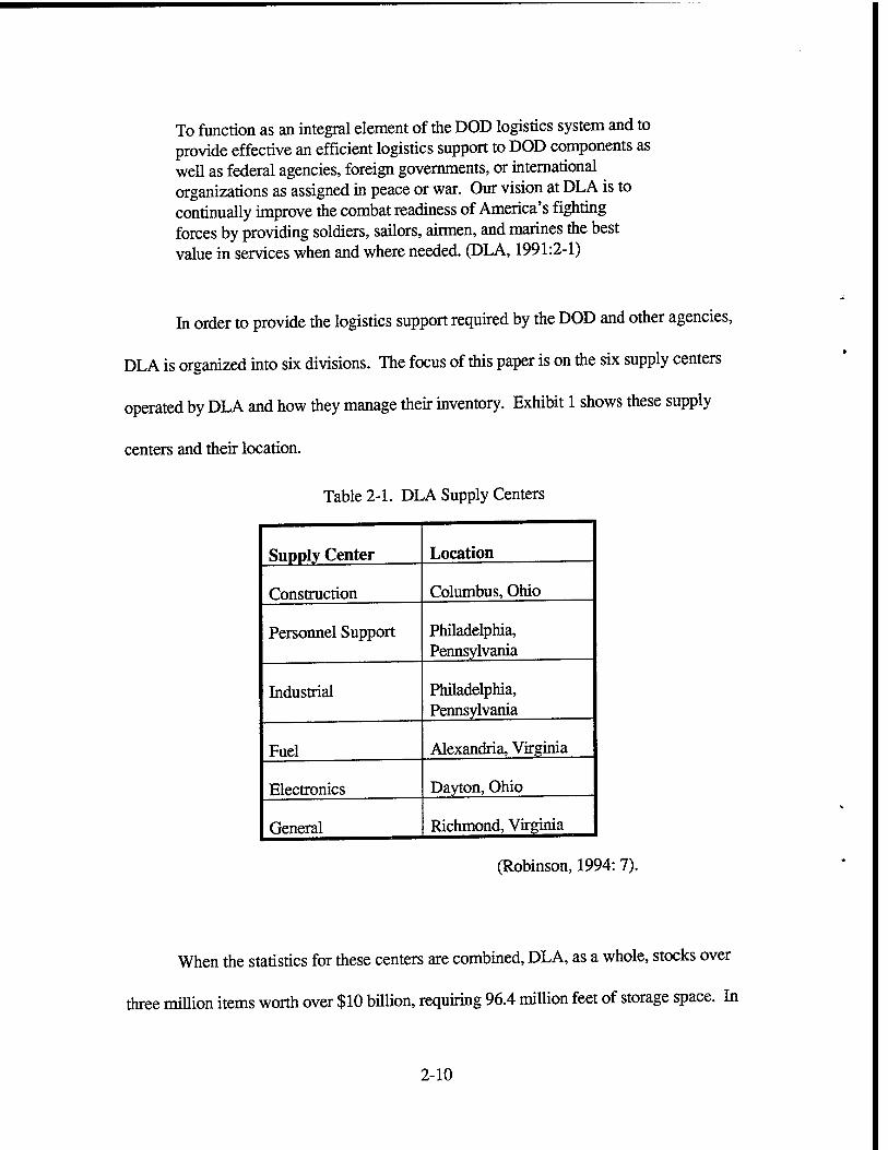
In order to provide the logistics support required by the DOD and other agencies,

DLA is organized into six divisions. The focus of this paper is on the six supply centers

operated by DLA and how they manage their inventory. Exhibit 1 shows these supply

centers and their location.

Table 2-1. DLA Supply Centers

Supply Center Location

Construction Columbus, Ohio

Personnel Support Philadelphia, Pennsylvania

Industrial Philadelphia, Pennsylvania

Fuel Alexandria, Virginia

Electronics Dayton, Ohio

General Richmond, Virginia

(Robinson, 1994: 7).

When the statistics for these centers are combined, DLA, as a whole, stocks over

three million items worth over $10 billion, requiring 96.4 million feet of storage space. In

2-10

addition, during 1991, these centers processed over 29 million requisitions while

maintaining an eighty-six percent stockage effectiveness rating (Robinson, 1994: 6).

Based on this data, one can see how crucial inventory management is to DLA in

supporting its customers.

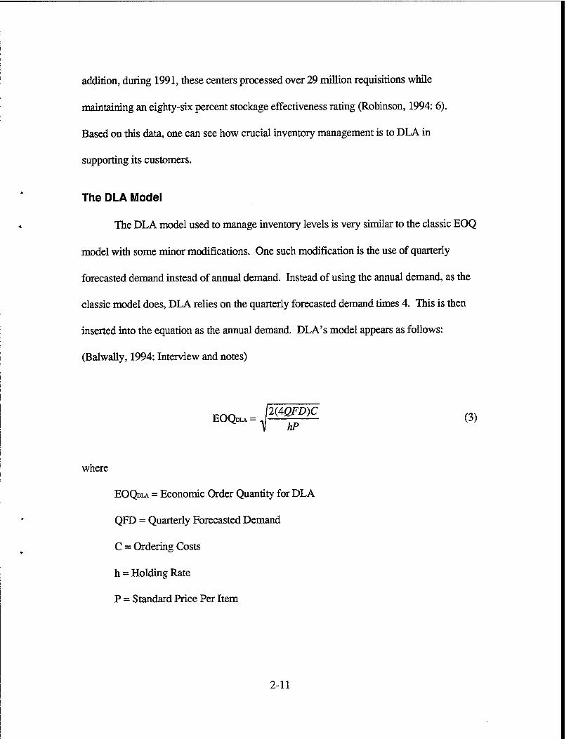
The DLA Model

The DLA model used to manage inventory levels is very similar to the classic EOQ

model with some minor modifications. One such modification is the use of quarterly

forecasted demand instead of annual demand. Instead of using the annual demand, as the

classic model does, DLA relies on the quarterly forecasted demand times 4. This is then

inserted into the equation as the annual demand. DLA's model appears as follows:

(Balwally, 1994: Interview and notes)

E0<^=JIffl£ (3) V hP

where

EOQDLA = Economic Order Quantity for DLA

QFD = Quarterly Forecasted Demand

C = Ordering Costs

h = Holding Rate

P = Standard Price Per Item

2-11

In addition, DLA factors out all the constants in the equation to reduce

computation time. For DLA, these constants are the ordering costs, the holding rate, and

the constant (2) used in the equation. (T) is then set equal to these constants. This

formula is as follows: (Balwally, 1994: Interview and notes)

\1C T = 2J— (4)

h

where

T = Constant Factor for DLA requirements model

C = Ordering Costs

h = Holding Costs

The DLA model is expressed as

EOQ = TJö^=|-VäD$ (5) V P 2P

where

EOQ = Economic Order Quantity

T = DLA's Constant Factor

QFD = Quarterly Forecasted Demand

P = Standard Price per Item

2-12

AD$ = Annual Predicted demand in dollars (AD$ = {4(QFD)p})

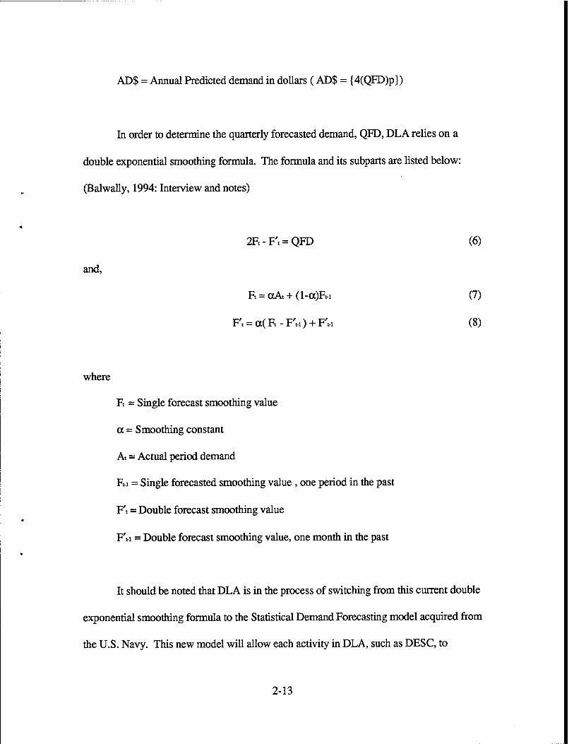
In order to determine the quarterly forecasted demand, QFD, DLA relies on a

double exponential smoothing formula. The formula and its subparts are listed below:

(Balwally, 1994: Interview and notes)

2Ft-F'« = QFD (6)

and,

Ft = aA. + (l-a)F.-i (7)

F« = a(R -F'M) + F'M (8)

where

Ft = Single forecast smoothing value

a = Smoothing constant

At = Actual period demand

Fti = Single forecasted smoothing value , one period in the past

F't = Double forecast smoothing value

F'M = Double forecast smoothing value, one month in the past

It should be noted that DLA is in the process of switching from this current double

exponential smoothing formula to the Statistical Demand Forecasting model acquired from

the U.S. Navy. This new model will allow each activity in DLA, such as DESC, to

2-13

determine its own forecasting method from the moving average to the double exponential

smoothing formula depending on which is a better predictor of future demand.

DLA also adds a variable safety level to the EOQ model. The appropriate level is

determined quarterly using a constrained optimization model which attempts to minimize

holding and ordering costs, given a target number of backorders (Balwally, 1994:

Interview and notes). Initially, DLA applies a Selective Management Category Code

(SMCC) to its items to differentiate between high dollar and frequency items and low

dollar and low frequency items. Exhibit 2 shows the SMCC categories.

Table 2-2. SMCC Categories

HIGH DOLLAR A C E LOW DOLLAR B D F

HIGH FREQUENCY

MEDR7M FREQUENCY

LOW FREQUENCY

(Bilikam, 1994)

Using simulation, DLA determines a multiplication factor, called essentiality, that

will maximize availability through safety level application in the most economical way.

Based on the simulation, categories A and B receive an essentiality factor of 6, category C

receive an essentiality factor of 2, and the other categories receive no essentiallity factor.

This factor, in basic terms, highlights the importance of having sufficient safety stock on

hand to avoid a stock out. This factor is then used in the calculation of the variable safety

stock level (Bilikam, 1994: Interview and notes).

2-14

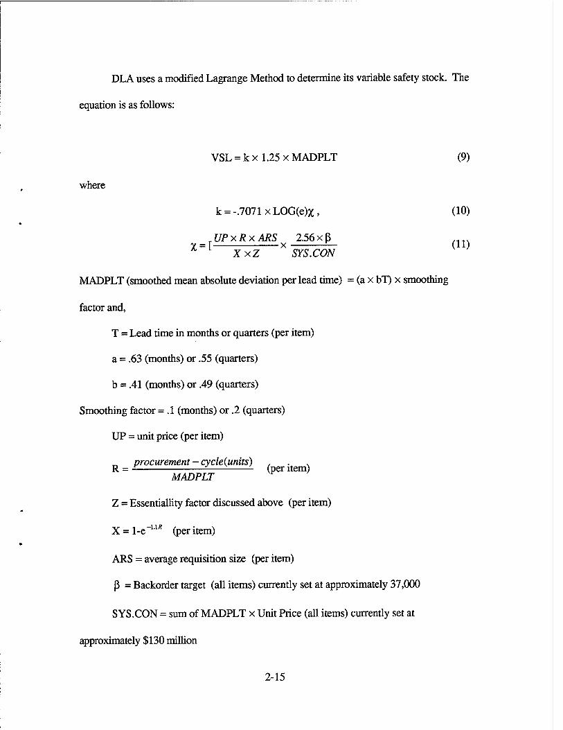
DLA uses a modified Lagrange Method to determine its variable safety stock. The

equation is as follows:

VSL = k x 1.25 x MADPLT (9)

where

k = -.7071xLOG(e)%, (10)

UPxRxARS 2.56xß Y = [ X — (11) A XxZ SYS.CON

MADPLT (smoothed mean absolute deviation per lead time) = (a x bT) x smoothing

factor and,

T = Lead time in months or quarters (per item)

a = .63 (months) or .55 (quarters)

b = .41 (months) or .49 (quarters)

Smoothing factor = .1 (months) or .2 (quarters)

UP = unit price (per item)

_ procurement - cycle(units) . . ~ MADPLT per l em

Z = Essentiallity factor discussed above (per item)

X = l-e"u* (per item)

ARS = average requisition size (per item)

ß = Backorder target (all items) currently set at approximately 37,000

SYS.CON = sum of MADPLT x Unit Price (all items) currently set at

approximately $130 million

2-15

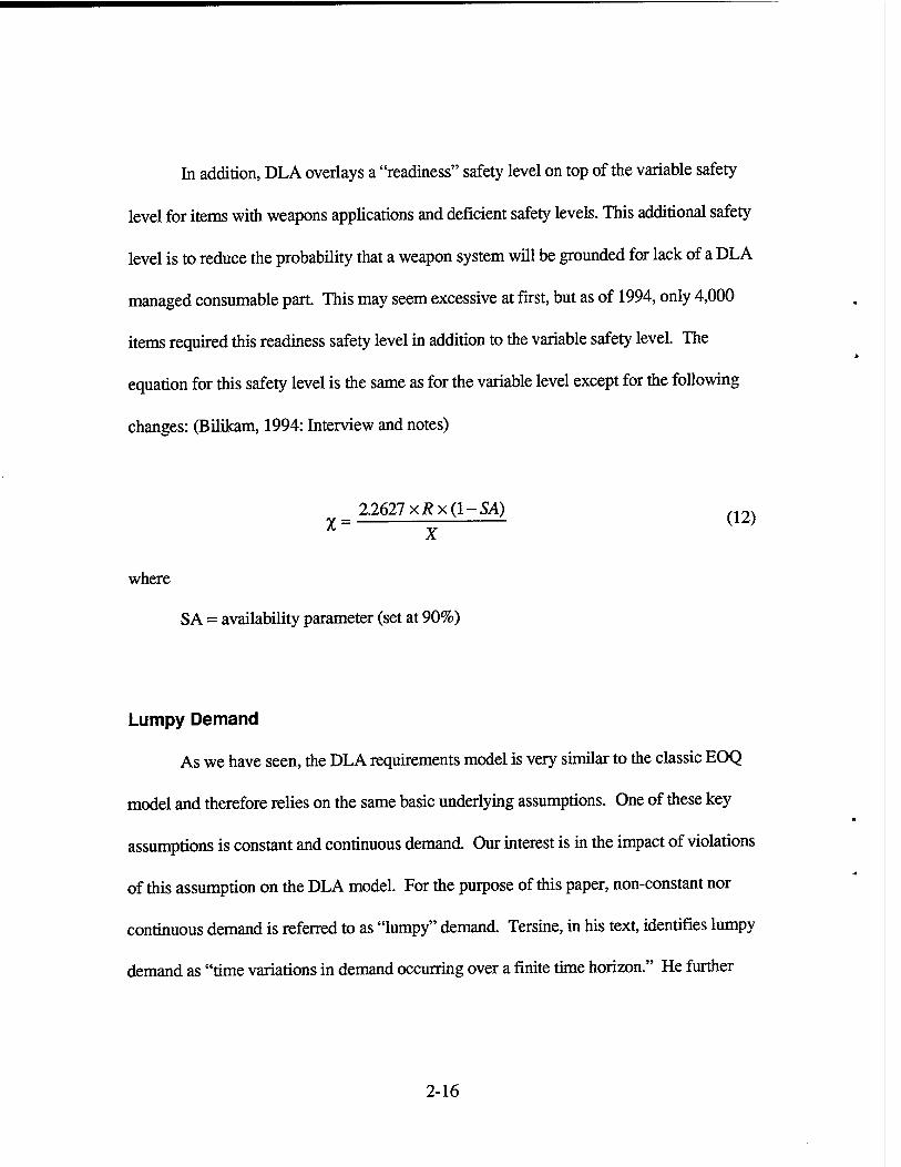
In addition, DLA overlays a "readiness" safety level on top of the variable safety

level for items with weapons applications and deficient safety levels. This additional safety

level is to reduce the probability that a weapon system will be grounded for lack of a DLA

managed consumable part. This may seem excessive at first, but as of 1994, only 4,000

items required this readiness safety level in addition to the variable safety level. The

equation for this safety level is the same as for the variable level except for the following

changes: (Bilikam, 1994: Interview and notes)

2.2627 XJRX(I-SA) n~ X = <12)

where

S A = availability parameter (set at 90%)

Lumpy Demand

As we have seen, the DLA requirements model is very similar to the classic EOQ

model and therefore relies on the same basic underlying assumptions. One of these key

assumptions is constant and continuous demand. Our interest is in the impact of violations

of this assumption on the DLA model. For the purpose of this paper, non-constant nor

continuous demand is referred to as "lumpy" demand. Tersine, in his text, identifies lumpy

demand as "time variations in demand occurring over a finite time horizon." He further

2-16

states that there are situations where lumpy demand is so pronounced that the constant

demand assumption is called into question. (Tersine, 1994:178)

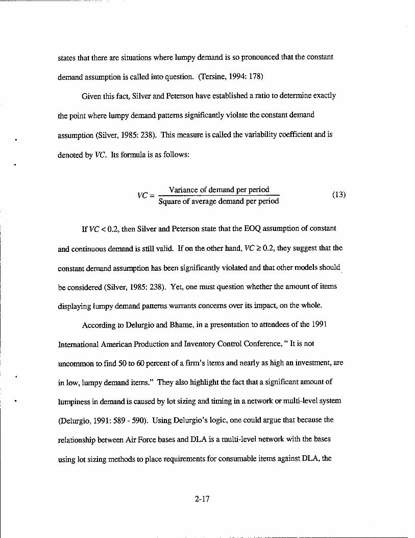
Given this fact, Silver and Peterson have established a ratio to determine exactly

the point where lumpy demand patterns significantly violate the constant demand

assumption (Silver, 1985: 238). This measure is called the variability coefficient and is

denoted by VC. Its formula is as follows:

_ Variance of demand per period Square of average demand per period

If VC < 0.2, then Silver and Peterson state that the EOQ assumption of constant

and continuous demand is still valid. If on the other hand, VC > 0.2, they suggest that the

constant demand assumption has been significantly violated and that other models should

be considered (Silver, 1985: 238). Yet, one must question whether the amount of items

displaying lumpy demand patterns warrants concerns over its impact, on the whole.

According to Delurgio and Bhame, in a presentation to attendees of the 1991

International American Production and Inventory Control Conference," It is not

uncommon to find 50 to 60 percent of a firm's items and nearly as high an investment, are

in low, lumpy demand items." They also highlight the fact that a significant amount of

lumpiness in demand is caused by lot sizing and timing in a network or multi-level system

(Delurgio, 1991:589 - 590). Using Delurgio's logic, one could argue that because the

relationship between Air Force bases and DLA is a multi-level network with the bases

using lot sizing methods to place requirements for consumable items against DLA, the

2-17

system itself would cause lumpiness in demand. Two USAF studies in this area found just

that.

In 1974, the Air Force Academy performed a study of the Air Force's EOQ

model. As a side note, they highlighted the fact that 64% of the consumable items they

sampled, exhibited other than normal demand patterns (Shields, 1990: 19 - 21). Again in

1985, Blazer verified that demand patterns tended to be lumpy in nature. Given that the

Air Force EOQ model expects a variance of demand to mean demand ratio of 3, Blazer

discovered, at the five bases he analyzed, this ratio varied from a low of 14.2 to a high of

29.5, illustrating the lumpiness of the demand patterns (Blazer, 1985: 11 -12).

Related Studies

Captains William Long and Douglas Engberson attempted to determine the effects

of violations of the constant demand assumption on DLA's requirements model. Using

simulation, they replicated DLA's requirements model and collected data on 540 stock

numbers managed by DESC. This data consisted of holding costs, ordering costs,

standard unit price, and quarterly demand data for the last 16 quarters. Based on the data

and the simulation model, Long and Engberson set up a complete 3x3x3 factorial

experimental design as follows (Long and Engberson, 1994:44):

Input Factors Levels

Ordering* 1. All activities order frequently (1 order per month) 2. Half the activities order frequently, Half infrequently) 3. All activities order infrequently (1 order every 6 months)

* the simulation model had four activities placing orders against DLA

Annual Demand 1. High (determined to be 3750 units based on data) (in units) 2. Medium (determined to be 481 units based on the data)

2-18

3. Low (determined to be 70 units based on the data)

Lead time 1. High (determined to be 14.4 months based on the data) (in months) 2. Medium (determined to be 7 months based on the data)

3. Low (determined to be 3.27 months based on the data)

The three response variables were established as total variable cost, average on

hand inventory, and pre-replenishment inventory. These three response variables were

used to determine the impact of lumpy demand on the costs associated with inventory for

DLA, as well as the ability of DLA to support customer requests. If lumpy demand causes

total variable costs to go up or customer support to go down, the appropriateness of

DLA's requirements model is called into question (Long and Engberson, 1994:46).

Long and Engberson intended to use the analysis of variance (ANOVA) statistical

method to evaluate the output of the simulation model to determine the impact of lumpy

demand. However, the variances between treatment means were not equal and this

violation of the ANOVA assumptions forced them to consider non-parametric statistical

methods. Because of the lack of independence between simulation runs, non-parametric

methods could not be used either. Practical observation of the output data was used to

made conclusions on the impact of lumpy demand. Based on their observations, Long and

Engberson determined that lumpy demand caused average on hand inventory to fluctuate

widely between periods. In addition, almost all pre-replenishment inventory levels were

negative, implying lumpy demand would require higher levels of safety stock than under

constant demand. They also determined that lead times and annual demand, when

combined with lumpy demand, have an impact on the on hand balances and overall

2-19

customer support. This led Long and Engberson to recommend further studies in this area

to quantify the impact of lumpy demand on DLA's requirements model (Long and

Engberson, 1994: 69-77). This study has served as the foundation for our current

research.

This chapter provided background information needed to understand the

importance and relevance of this research. Reasons for holding inventory as well as the

costs associated with inventory were described. In addition, the components of the

classical EOQ model and the DLA requirements model were outlined. Finally, the

concept of lumpy demand was presented and past relevant research was discussed. The

following chapter will discuss the proposed methodology to analyze the impact of lumpy

demand on DLA's model.

2-20

III. Methodology

This chapter will discuss the methodology chosen to answer the research questions

posed in Chapter I. In order to ensure all aspects of the research are discussed, this

chapter will be organized according to the seven steps Cooper and Emory have established

as essential to successful experiments (Cooper and Emory, 1995: 353).

Conducting An Experiment

The method chosen for this research is experimentation. Experimentation is

defined as "a study involving the intervention by the researcher beyond that required for

measurement" (Cooper and Emory, 1994: 351). The researcher attempts to manipulate

the independent variables and then record the effect of the manipulation on the dependent

variables. There are four distinct advantages of experimentation. The first advantage is

the researcher's ability to manipulate the independent variable to determine the effect on

the dependent variable. The second advantage is that the effect of extraneous variables

can be removed from the experiment. The third advantage is that cost and convenience of

the experiment is superior to other methods. The fourth advantage is the ability to

replicate an experiment to verify results (Cooper and Emory, 1994: 352).

To make experimentation a success, a researcher must complete a series of

activities in a logical manner in order to ensure the experiment's success. According to

Cooper and Emory, there are seven specific activities that a researcher must follow in

3-1

order to guard against defects in the experiment and its results. Those seven activities are

listed below: (Cooper and Emory, 1995: 353 - 370)

1. Select relevant variables

2. Specify the level(s) of the treatments

3. Control the experimental environment

4. Choose the experimental design

5. Select and assign the subjects

6. Pilot test, revise, and test

7. Analyze the data

The remainder of this chapter will focus on applying each of these activities to this

study to establish a concrete foundation to determine the results and subsequent

conclusions.

Selecting Relevant Variables

The focus of research is to answer a question that is not readily answerable based

on current knowledge. As such, the research question establishes what relevant variables

will be required for the experiment. For this research, the question , as stated in Chapter I,

is "What is the impact of violations of the constant demand assumption on DLA's

requirements model?". More specifically, the experiment must answer the following three

questions:

3-2

1. How does lumpy demand affect the total variable cost portion of DLA's

requirements model?

2. How does lumpy demand affect DLA's requirements model in regard to

inventory levels maintained at DLA?

3. Is there a better model that could be used instead of the current requirements

model used by DLA?

The answers to these questions will provide a picture of the total impact of lumpy

demand on DLA's model and ultimately, the appropriateness of the model under these

conditions. In order to establish and measure the impact of lumpy demand, the relevant

performance measures for the experiment must be identified. Two performance measures

were established as relevant and important. They are total variable cost and average on-

hand inventory at DLA.

Total variable cost is an important measure in evaluating the EOQ model. The

EOQ model attempts to balance ordering and holding costs to minimize total variable

costs. Therefore, if the total variable cost under lumpy demand was significantly different

than under constant and continuous demand, the impact of lumpy demand on the model

would be demonstrated as being significant.

Another important performance measure is average on hand inventory. It provides

a gauge of how much inventory the model requires to satisfy demand. If it can be shown

that the average on hand inventory under lumpy demand is significantly different than

under constant and continuous demand, given the overall annual demand is the same under

3-3

both conditions, one could argue that the lumpy demand has an observable impact on the

model.

Factors and Levels of Treatment

Factors and levels of treatments for this research were determined based on

knowledge of the EOQ model, the documented research of Long and Engberson, and the

characteristics of the data sample collected from the Defense Electronics Supply Center.

Before discussing each of these factors and its appropriate levels, it is important to

describe the data collection procedures used to develop the characteristics for these

factors.

In order to determine the DLA specific characteristics for these factors, a sample

of 525 national stock numbers was collected by DESC personnel for this research.

According to Mr. Balwally and Mr. Bilikam, operations analysts at DESC, this sample is

representative of the demand patterns that all of DLA's EOQ managed items face. The

data collected included the national stock number for each unit, the past sixteen quarters

of demand data, the calculated quarterly forecasted demand, the lead time, and the

nomenclature. This data was then used to determine the characteristics or levels for the

factors for this research. Appendix A provides an example of the data that was collected.

Using the collected data, factors and levels of treatment were established. Long

and Engberson, in their experiment on the effect of lumpy demand on DLA's requirements

model, used demand patterns, annual demand, and total lead time as their factors.

Initially, this study began on the assumption that Long and Engberson's three factors and

3-4

levels would be used to replicate their experiment. These factors and levels are listed in

Table 3-1. However, preliminary analysis of the DLA data made it apparent that these

factors and levels would not be appropriate for this study.

The first factor established by Long and Engberson was demand pattern. They

used three levels to represent constant and continuous demand, lumpy demand, and a

mixture of the two. For the purpose of this research, it was decided that demand is either

constant and continuous or lumpy in nature. Although demand patterns may vary between

these two patterns during a given time period, the objective of this research is to determine

the impact of lumpy demand on DLA's model. Therefore, levels of demand pattern will

be either constant and continuous or lumpy. Using Silver and Peterson's definition of

lumpy demand provided in Chapter n, lumpy demand patterns will be such that the

variance of demand divided by the mean demand squared will be greater than 0.20 (Silver,

1985: 238). Based on the sample data, 95.38% of items DLA manages exhibit lumpy

demand patterns. On the other hand, constant and continuous demand will be such that

the variance to mean squared ratio is less than 0.20. Appendix I illustrates these

calculations on a sample of a few items to give the reader a better understanding of what

would be considered lumpy and what would be considered constant and continuous.

A second factor used by Long and Engberson in determining the impact of lumpy demand

was the annual demand placed on DLA. This annual demand is in units. They

hypothesized that in order to determine the appropriateness of DLA's model under lumpy

demand, one must account for the different annual demands that are placed against DLA

and its impact on the model. There is the possibility that the model will react differently

under lumpy demand with varying levels of annual demand. In order to evaluate these

3-5

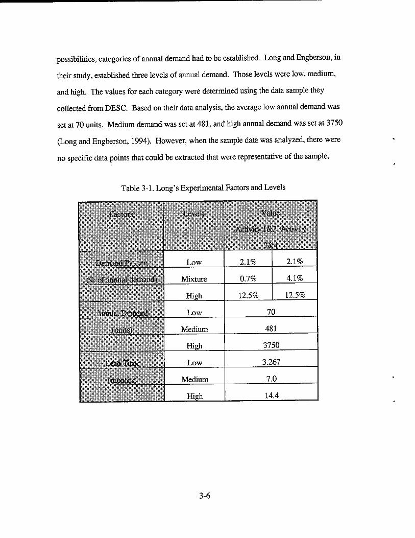
possibilities, categories of annual demand had to be established. Long and Engberson, in

their study, established three levels of annual demand. Those levels were low, medium,

and high. The values for each category were determined using the data sample they

collected from DESC. Based on their data analysis, the average low annual demand was

set at 70 units. Medium demand was set at 481, and high annual demand was set at 3750

(Long and Engberson, 1994). However, when the sample data was analyzed, there were

no specific data points that could be extracted that were representative of the sample.

Table 3-1. Long's Experimental Factors and Levels

-■ ;;:FaCtOTS ■: Levels. ;:V-- Value-';

::.:. Activity-1&2 Activity ■

3*4

Demand Pattern Low 2.1% 2.1%

C% of annual demand) Mixture 0.7% 4.1%

'.'V: ' ' .'.:•: :"^:: .■■?'.'\ ' ' " '"

High 12.5% 12.5%

Annual Demand Low 70

Medium 481

High 3750

Lead Time Low 3.267

(months) Medium 7.0

High 14.4

3-6

Appendix B, a graph of the quarterly demand pattern from the collected sample,

illustrates the problem encountered in extracting specific data points. Because the graph

appears to represent a exponential distribution with a long tail of large but infrequent

orders, there were no natural breaks in the data to categorize it into levels of demand.

SAS/STAT Release 6.03, a statistical software package, was then used to analyze the data

and locate any clusters of data points which could be used as levels. The results of the

cluster analysis indicated that there were no clusters in the data collected. Therefore, the

observed data pattern was validated with Mr. Michael Pouy, headquarters DLA. He

agreed that the demand pattern DLA faces fits the exponential distribution with a long

sparsely populated tail. Based on this information and the inability of the cluster analysis

to find natural levels in the data, annual demand was eliminated as a factor and allowed to

fluctuate according to a exponential distribution with the parameters extracted from the

collected data to reflect the actual demand pattern.

The third factor Long and Engberson chose for this experiment was lead time.

Long and Engberson determined that lead time could be divided into three categories:

low, medium, and high. Based on the data, low lead time averaged 3.267 months, medium

lead time averaged 7.0 months, and long lead time averaged 14.4 months. As with the

annual demand, this study's analysis of the data provided different results. Using the data

collected from DESC, an attempt was made to determine natural levels of lead times. This

analysis uncovered a distribution of lead times that appeared to fit an exponential

distribution with a long sparsely populated tail similar to the annual demand distribution

discussed above.

3-7

Therefore, SAS/STAT Release 6.03 was used to analyze the data and locate any

clusters of data points which could be used as levels. According to SAS output results,

there were no clusters in the data collected. Again, DLA was contacted to determine if

they had specific categories of lead times to indicate short and long lead times. If specific

numbers could be assigned to these categories, they could then serve as DLA determined

breaks in the data. Unfortunately, it was discovered that there is no such categorization of

lead times at DLA. After further examination of the data and based on the preliminary

data, it was determined that lead time was not a factor in this experiment. Failure to

categorize the lead times was not the reason for its elimination. Lead time was not a

factor for two reasons. First, lead time only impacts the EOQ model in the safety stock

and reorder point calculations. From the beginning, safety stock was eliminated from this

experiment because it could hide the real impact of lumpy demand on DLA's requirements

model. After all, the purpose of safety stock is to protect the organization from

fluctuations in demand. The reorder point then, without safety stock, is simply the mean

demand during lead time. This leads to the second point. This research does not use

customer service levels as a performance measure; therefore, changing the reorder point

by varying lead times does not provide any insight into the impact of lumpy demands being

placed against DLA's requirements model and could actually confound the results if it

were allowed to vary. For these reasons, it was decided to hold the lead time for DLA

from its suppliers constant throughout the experiment at 100 days. This figure was

determined based on the data collected from DESC. Appendix J provides a graph of the

leadtimes from the collected data..

3-8

Experimental Environment

The control of the environment refers to the ability of the researcher to minimize

his impact on the environment and the impact of all extraneous variables to the

experiment. Simulation, the methodolgy chosen for this research, inherently reduces the

impact of both of these problems on the experiment. An in-depth analysis of exactly how

simulation aids in the control of the experimental environment will be discussed as part of

the next section.

Experimental Design

The method chosen for this research is simulation. Simulation, as defined by

Pritsker, is "the process of designing a mathematical - logical model of a real system and

experimenting with this model on a computer" (Pritsker, 1986: 6). There are several

advantages of studying a system in this manner. First, the system can be tested and

manipulated before incurring the cost of actually building the system. Secondly, the

system can be studied without bringing the existing system off-line. Finally, one avoids

the potential of damaging or destroying the existing system through testing procedures

(Pritsker, 1986: 6). The last two advantages are relevant to this study. Because the DLA

requirements model is continually being used to determine requirements and manage

transactions, it would be impractical to bring this system off-line for our experiment. In

addition, the potential costs associated with any down time in the system prohibit direct

manipulation of the DLA requirements model.

3-9

The use of simulation for inventory related issues is not new. Andrew Clark, in his

article, "The Use of Simulation to Evaluate a Multiechelon, Dynamic Inventory Model,"

highlights examples where simulation is the only real method available to solve complex

inventory issues (Clark, 1993: 429-444). In addition, Choi, Malstrom, and Tsai, used

simulation to evaluate several lot sizing methods within multilevel inventory systems, to

include the EOQ model. This analysis of the lotsizing methods was performed to establish

a ranking of the effectiveness of the lot-sizing methods (Choi, Malstrom, and Tsai, 1988:

4-10).

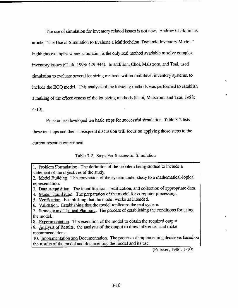
Pritsker has developed ten basic steps for successful simulation. Table 3-2 lists

these ten steps and then subsequent discussion will focus on applying those steps to the

current research experiment.

Table 3-2. Steps For Successful Simulation

1. Problem Formulation. The definition of the problem being studied to include a statement of the objectives of the study. 2. Model Building. The conversion of the system under study to a mathematical-logical representation. 3. Data Acquisition. The identification, specification, and collection of appropriate data. 4. Model Translation. The preparation of the model for computer processing. 5. Verification. Establishing that the model works as intended. 6. Validation. Establishing that the model replicates the real system. 7. Strategic and Tactical Planning. The process of establishing the conditions for using the model. 8. Experimentation. The execution of the model to obtain the required output. 9. Analysis of Results, the analysis of the output to draw inferences and make recommendations. 10. Implementation and Documentation. The process of implementing decisions based on the results of the model and documenting the model and its use.

(Pritsker, 1986: 1-10)

3-10

Problem Formulation. The problem this research attempts to resolve is the

appropriateness of DLA's requirements model under lumpy demand patterns. The

research questions are stated in Chapter I and earlier in this chapter.

Model Building. Simulation models will be created using Pritsker's SLAM II

software (Version 4.4) on the Digital Equipment Corporation's VAX 6420 mainframe

computer. These models will then be compiled and linked using DEC VAX FORTRAN

Compiler (Version 6.1). The purpose of these models is to replicate the DLA

requirements model under lumpy demand so that the researchers can statistically

determine the impact of lumpy demand. A total of four models will be built using

SLAMSYS (Version 4.0).

Each of the four models will reflect will represent different assumptions of the

demand pattern DLA faces. The first model is referred to as the Normal, Constant and

Continuous model and reflects all the assumptions of the EOQ model that DLA uses for

their requirements computations. As such, demand is generated from the bases and sent

to DLA on a deterministic schedule. This implies that each bases orders the same quantity

during a set period. The second model is called the Normal Demand model. It is similar

to the previous model except it relaxes the assumption of constant and continuous demand

to allow the amount of an item ordered by the bases to vary according to a normal

distribution. Most inventory text books use this assumption of a normal distribution of

demand when applying the EOQ model to real situations. This assumption is generally

true for a majority of the consumable items (Tersine, 1994: 212).

3-11

The third model is called the Lumpy demand model. This model incorporates

DLA's requirements model like the previous models, except demand from the bases is

allowed to fluctuate. The demand faced by DLA comes from a exponential distribution,

as reflected in the sample from DESC, and the timing of the demand comes from a normal

distribution. This model is reflective of the current conditions that DLA operates in. The

fourth model is the same as the Lumpy demand model except the EOQ model that DLA

uses is replaced with the Silver-Meal model which is designed to more effectively handle

lumpy demand. Table 3-3 summarizes the comparisons of the models.

Table 3-3. Comparison of Models

Model Timing of demands from bases

Quantity of each order

Requirements Model used

Normal, Constant and Continuous

Orders placed every month

8 units per order DLA's EOQ model

Normal Demand Orders placed every month

Normal distribution with mean of 8 and standard deviation ofl

DLA's EOQ model

Lumpy Demand Triangular distribution with a mean of 90 days, a max of 150, and a min of 30 days

Exponential distribution with mean of 89.36543

DLA's EOQ model

Silver-Meal Triangular distribution with a mean of 90 days, a max of 150, and a min of 30 days

Exponential distribution with mean of 89.36543

Silver-Meal model

Data Acquisition. As mentioned earlier in this chapter, data was collected from

DESC to establish the parameters for the independent variables in the model. Table 3-3

outlines the values chosen for the variables. These values will be incorporated into the

3-12

Simulation model. As discussed in Chapter II, DLA uses a Lagrangean method to

determine its variable safety stock. For the purpose of this experiment, the variable safety

stock will not be included in the simulation model. It was determined that safety stock

might mask the impact of lumpy demand on the model. Long and Engberson, in then-

experiment, eliminated safety stock from their experiment for the same reason.

Model Translation. Appendix C provides a detailed discussion of the simulation

model to include the program logic.

Verification. The verification of the models was completed in two steps. In the

first step, the authors went step by step through the code to ensure that it worked as it

was designed to. Also, the authors relied on the SLAMSYS (Version 4.4) syntax check

and the DEC VAX FORTRAN Compiler (Version 6.1) to aid in validating the program

code and fortran code. Secondly, a pilot test of five runs for each model was

accomplished. Results of the runs were analyzed to determine if the models were working

properly. This process was repeated until the models were working properly.

Validation. The models were validated by inventory instructors at the Air Force

Institute of Technology (AFIT) and personnel at DLA. First, personnel at DESC were

interviewed to determine any specific DLA policies that needed to be reflected in the

model (Balwally, 1994: Interview). Next, the issues raised by the DESC personnel were

discussed with the inventory instructors at AFIT. Each model was analyzed to ensure it

reflected DLA's inventory system, applicable DLA policies, and the assumptions implied

by each model's environment.

3-13

Strategie and Tactical Planning. Before each model can be run to collect the

required data, three very important questions must be answered. They concern initial

starting conditions, how long the model should be run for each run, and how many

samples or runs need to be made to ensure that the collected data is reflective of its

population. All of these questions will be answered next.

First, the initial starting conditions for each model had to be determined. The

models called for customers to begin placing demands to DLA as soon as the model

started. This means that unless the model began with some inventory at DLA, it would

backorder immediately. Secondly, until after the first quarter, there is no forecasted

demand to use in determining order quantities. Therefore, the initial amount of inventory

on hand was set at a rough-cut EOQ amount. Also, the forecasted demand was set at this

same amount. Appendix C provides specific details on these initial conditions. These

predetermined starting conditions allow the model to start at a more steady state but do

not impact the collected data from the model, as we will see next.

The second question raised earlier concerned the length of time the models should

be run. One of the assumptions of simulation models is that the output reflects the system

in steady state. Yet, with many models there is a warm up period, also called the transient

period, where the model is moving toward steady state but the model output is still

affected by the initial starting conditions. If this transient period were included in the

output of the model it might bias the results because it doesn't reflect the true steady state

of the system. Therefore, modelers must attempt to determine where the transient period

3-14

ends so that the observations during the transient period can be deleted (Law and Kelton,

1991: 545).

One method to estimate the beginning of steady state is to use a pilot ran from

each model and apply a moving average to the periodic output on the measured variable.

When the graphed moving averages are analyzed, steady state begins as the moving

average curve levels off (Law and Kelton, 1991: 545-551). This was the method used to

determine the end of the transient phase for this experiment. Appendix D provides the

graphs of average inventory and total variable cost over time. The longest transient phase

lasted 55 years or 19,800 days (days are used in the simulation, but the output is per year).

In order to ensure that the model was in steady state, all statistical arrays were cleared at

20,000 days. The model was then allowed to ran for an additional 20,000 time units for

data collection purposes. Therefore, the overall lenght of each ran was set at 40,000 days

or 111 years.

The third question raised earlier concerned the number of runs required of each

model to ensure meaningful output data. In order to determine the correct sample size

necessary for the experiment, a sample of five runs was produced from each model. The

models were lumpy demand with the EOQ, normal demand with the EOQ, and lumpy

demand with the Silver and Meal model. The constant and continuous model is

deterministic and therefore does not require a sample size calculation. The standard

deviation of the five runs was calculated and used as part of the calculation of sample size.

Next, a level for a and ß level were determined. The a level is the probability of a

type one error or stated otherwise, the probability of rejecting the null hypothesis when it

3-15

is true. The a for this experiment was set at 0.05. The ß level is the probability of a type

two error. This occurs when you accept the null hypothesis when it is false. Based on

discussions with AFIT statistics instuctors, ß was set at 0.05. Finally, a value for <j> must

be established. ()> reflects the amount of the acceptable difference between the true mean

and the observed mean divided by the standard deviation of the sample. The acceptable

difference was set at 20 units to keep the sample size manageable while maintaining

acceptable levels for a and ß. These parameters were then used to determine the sample

size required from Table All, page 632 of Statistical Design and Analysis of Experiments

with Applications to Engineering and Science by Mason, Gunst, and Hess. Based on the

chart, the highest required runs was 24. Therefore the number of runs was set at 30.

Appendix E provides the computations associated with this process.

Experimentation. Appendix C provides a detailed explanation of how the models

were run. A discussion of the logical flow of each model to include the specific functions

of the various subparts is given. In addition, the simulation code and Fortran subroutines

for each model are provided.

Analysis of Results. The analysis of results will be discussed in detail in a

subsequent section titled "Analyze the Data." Specifically, the analysis will be divided into

two parts. Part one will be a check for normality of the output data. Based on the results

of this test, parametric or nonparametric procedures will be used to determine if the

hypotheses will be rejected.

3-16

Implementation and Documentation. Appendix C provides all documentation on

each model and its code. Any recommendations for implementation will be discussed in

detail in Chapter V of this thesis.

Select and Assign the Subjects

The focus of this portion of the experiment is on ensuring that the subjects are

representative of the population. The subjects for this simulation are the demand patterns

created during the simulation process. The question to be answered is whether they are

representative of the population demand patterns that DLA faces. The demand patterns

created in the simulation are derived from the sample collected by DESC personnel. The

goal of the DESC personnel during this collection of data was to collect a representative

sample of the demand patterns DLA faces. Therefore, it is assumed that the demand

patterns created in the simulation are reflective of the population of demand patterns DLA

faces.

Testing Data

This section refers to the verification and validation process. A pilot test of our

simulation model will be conducted to ensure the model accurately represents the DLA

consumable item environment. The Long and Engberson study concluded that verification

and validation involved the coordination and review of AFIT instructors and experts from

DESC. We have chosen the same method of verification and validation. A pilot test of

five runs will be used for this process.

3-17

Analyze the Data

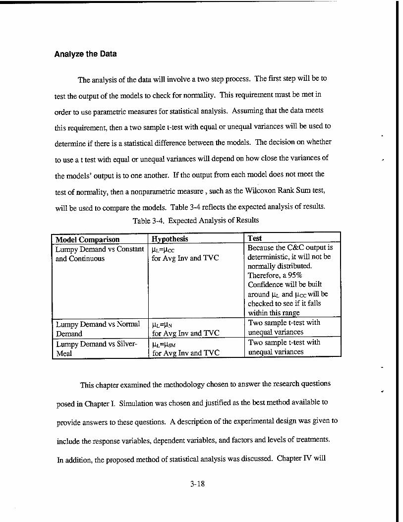
The analysis of the data will involve a two step process. The first step will be to

test the output of the models to check for normality. This requirement must be met in

order to use parametric measures for statistical analysis. Assuming that the data meets

this requirement, then a two sample t-test with equal or unequal variances will be used to

determine if there is a statistical difference between the models. The decision on whether

to use a t test with equal or unequal variances will depend on how close the variances of

the models' output is to one another. If the output from each model does not meet the

test of normality, then a nonparametric measure, such as the Wilcoxon Rank Sum test,

will be used to compare the models. Table 3-4 reflects the expected analysis of results.

Table 3-4. Expected Analysis of Results

Model Comparison Lumpy Demand vs Constant and Continuous

Lumpy Demand vs Normal Demand Lumpy Demand vs Silver- Meal

Hypothesis UL=HCC

for Avg Inv and TVC

HJ=HN for Avg Inv and TVC

M-L=M-SM

for Avg Inv and TVC

Test Because the C&C output is deterministic, it will not be normally distributed. Therefore, a 95% Confidence will be built around (iL and [ice will be checked to see if it falls within this range Two sample t-test with unequal variances Two sample t-test with unequal variances

This chapter examined the methodology chosen to answer the research questions

posed in Chapter I. Simulation was chosen and justified as the best method available to

provide answers to these questions. A description of the experimental design was given to

include the response variables, dependent variables, and factors and levels of treatments.

In addition, the proposed method of statistical analysis was discussed. Chapter IV will

3-18

now discuss the actual execution of the experiment and the subsequent analysis of the

results. Chapter V will then provide conclusions and recommendations based on the

results discussed in Chapter IV.

3-19

IV. Data Analysis

This chapter discusses the simulation output data and explains the statistical

techniques used to analyze the data. First, the proposed statistical analysis techniques will

be presented. Next, the assumptions of these techniques and the validation that the

experiment met these assumptions will be discussed. Finally, the output data will be

analyzed and comparisons between models will be made.

Proposed Statistical Analysis

In Chapter III, the proposed statistical analysis technique was the two-sample t-

test with unequal variances. The assumption that accompanies that test is that the two

populations from which the samples were collected are normally distributed (Montgomery,

1991: 30). In order to confirm the assumption of normality, the output from each model

was tested using the Wilkes-Shapiro test. This test was performed using Statistics,

Version 4.0. Using a sample size of 30 and an alpha of 0.05, the critical value for the test

was determined from Table All, page 632, of Statistical Design and Analysis of

Experiments with Applications to Engineering and Science by Mason, Gunst, and Hess.

Based on the critical value from the chart and the calculated values from the samples, all

the samples, except the Constant and Continuous model, exceeded the critical value and

therefore, can be assumed to be normally distributed. Appendix F contains the scores of

each of the samples and the critical value from Table All.

4-1

The Constant and Continuous model is a deterministic model and cannot meet the

assumption of normality. By deterministic, it is meant that the results are the same for

every run of the model. Therefore, in order to compare any of the other models to it, one

must build a confidence interval around the mean of the output that is being compared to

the results of the Constant and Continuous model. The hypothesis being tested is that the

mean of the sample is equal to the answer derived from the Constant and Continuous

model. If the Constant and Continuous model's result is not within this confidence

interval, then the hypothesis of equal means is rejected. This requires that the sample

being compared to the Constant and Continuous model come from a population that is

normally distributed. As mentioned earlier, all of the other models passed the test for

normality. Therefore, this assumption has been met.

Output Data Analysis

Data was collected from the simulation models for the response variables, average

on-hand inventory and total variable cost. This data was then used to make comparisons

between models. The following discussion is organized by variable and then by model

comparison.

Average On-Hand Inventory. Average on-hand inventory represents the average

amount of inventory maintained at DLA. Table 4-1 highlights the mean value for average

on-hand inventory for each model.

The first test conducted was a comparison between the Constant and Continuous

model and the Lumpy Demand model. The Constant and Continuous model represents

4-2

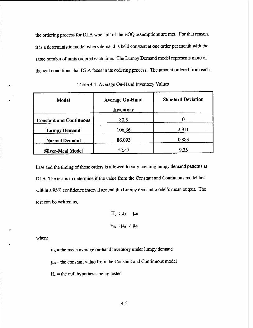
the ordering process for DLA when all of the EOQ assumptions are met. For that reason,

it is a deterministic model where demand is held constant at one order per month with the

same number of units ordered each time. The Lumpy Demand model represents more of

the real conditions that DLA faces in its ordering process. The amount ordered from each

Table 4-1. Average On-Hand Inventory Values

Model Average On-Hand

Inventory

Standard Deviation

Constant and Continuous 80.5 0

Lumpy Demand 106.36 3.911

Normal Demand 86.093 0.883

Silver-Meal Model 52.47 9.35

base and the timing of those orders is allowed to vary creating lumpy demand patterns at

DLA. The test is to determine if the value from the Constant and Continuous model lies

within a 95% confidence interval around the Lumpy demand model's mean output. The

test can be written as,

Ho : |1A = M-B

HA : HA * ^B

|IA = the mean average on-hand inventory under lumpy demand

(XB = the constant value from the Constant and Continuous model

Ho = the null hypothesis being tested

where

4-3

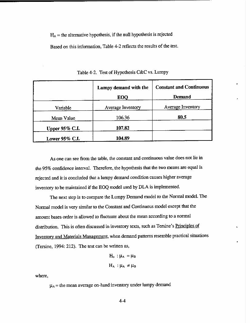
HA = the alternative hypothesis, if the null hypothesis is rejected

Based on this information, Table 4-2 reflects the results of the test.

Table 4-2. Test of Hypothesis C&C vs. Lumpy

Lumpy demand with the

EOQ

Constant and Continuous

Demand

Variable Average Inventory Average Inventory

Mean Value 106.36 80.5

Upper 95% C.I. 107.82

Lower 95% C.I. 104.89

As one can see from the table, the constant and continuous value does not lie in

the 95% confidence interval. Therefore, the hypothesis that the two means are equal is

rejected and it is concluded that a lumpy demand condition causes higher average

inventory to be maintained if the EOQ model used by DLA is implemented.

The next step is to compare the Lumpy Demand model to the Normal model. The

Normal model is very similar to the Constant and Continuous model except that the

amount bases order is allowed to fluctuate about the mean according to a normal

distribution. This is often discussed in inventory texts, such as Tersine's Principles of

Inventory and Materials Management, when demand patterns resemble practical situations

(Tersine, 1994: 212). The test can be written as,

Ho : (IA = M«

HA : HA *■ HB

where,

|iA= the mean average on-hand inventory under lumpy demand

4-4

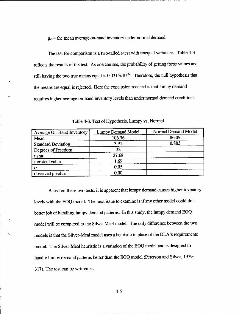
HB = the mean average on-hand inventory under normal demand

The test for comparison is a two-tailed t-test with unequal variances. Table 4-3

reflects the results of the test. As one can see, the probability of getting these values and

still having the two true means equal is 0.0315xl0"22. Therefore, the null hypothesis that

the means are equal is rejected. Here the conclusion reached is that lumpy demand

requires higher average on-hand inventory levels than under normal demand conditions.

Table 4-3. Test of Hypothesis, Lumpy vs. Normal

Average On-Hand Inventory Lumpy Demand Model Normal Demand Model

Mean 106.36 86.09

Standard Deviation 3.91 0.883

Degrees of Freedom 32 tstat 27.68 t-critical value 1.69

a 0.05 observed p value 0.00

Based on these two tests, it is apparent that lumpy demand causes higher inventory

levels with the EOQ model. The next issue to examine is if any other model could do a

better job of handling lumpy demand patterns. In this study, the lumpy demand EOQ

model will be compared to the Silver-Meal model. The only difference between the two

models is that the Silver-Meal model uses a heuristic in place of the DLA's requirements

model. The Silver-Meal heuristic is a variation of the EOQ model and is designed to

handle lumpy demand patterns better than the EOQ model (Peterson and Silver, 1979:

317). The test can be written as,

4-5

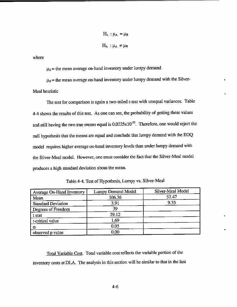
Ho : |IA = Mß

HA : HA *■ HB

where

|iA = the mean average on-hand inventory under lumpy demand

HB = the mean average on-hand inventory under lumpy demand with the Silver-

Meal heuristic

The test for comparison is again a two-tailed t-test with unequal variances. Table

4-4 shows the results of this test. As one can see, the probability of getting these values

and still having the two true means equal is 0.0225x10"22. Therefore, one would reject the

null hypothesis that the means are equal and conclude that lumpy demand with the EOQ

model requires higher average on-hand inventory levels than under lumpy demand with

the Silver-Meal model. However, one must consider the fact that the Silver-Meal model

produces a high standard deviation about the mean.

Table 4-4. Test of Hypothesis, Lumpy vs. Silver-Meal

Average On-Hand Inventory Lumpy Demand Model Silver-Meal Model Mean 106.36 52.47 Standard Deviation 3.91 9.35 Degrees of Freedom 39 tstat 29.12 t-critical value 1.69 a 0.05 observed p value 0.00

Total Variable Cost. Total variable cost reflects the variable portion of the

inventory costs at DLA. The analysis in this section will be similar to that in the last

4-6

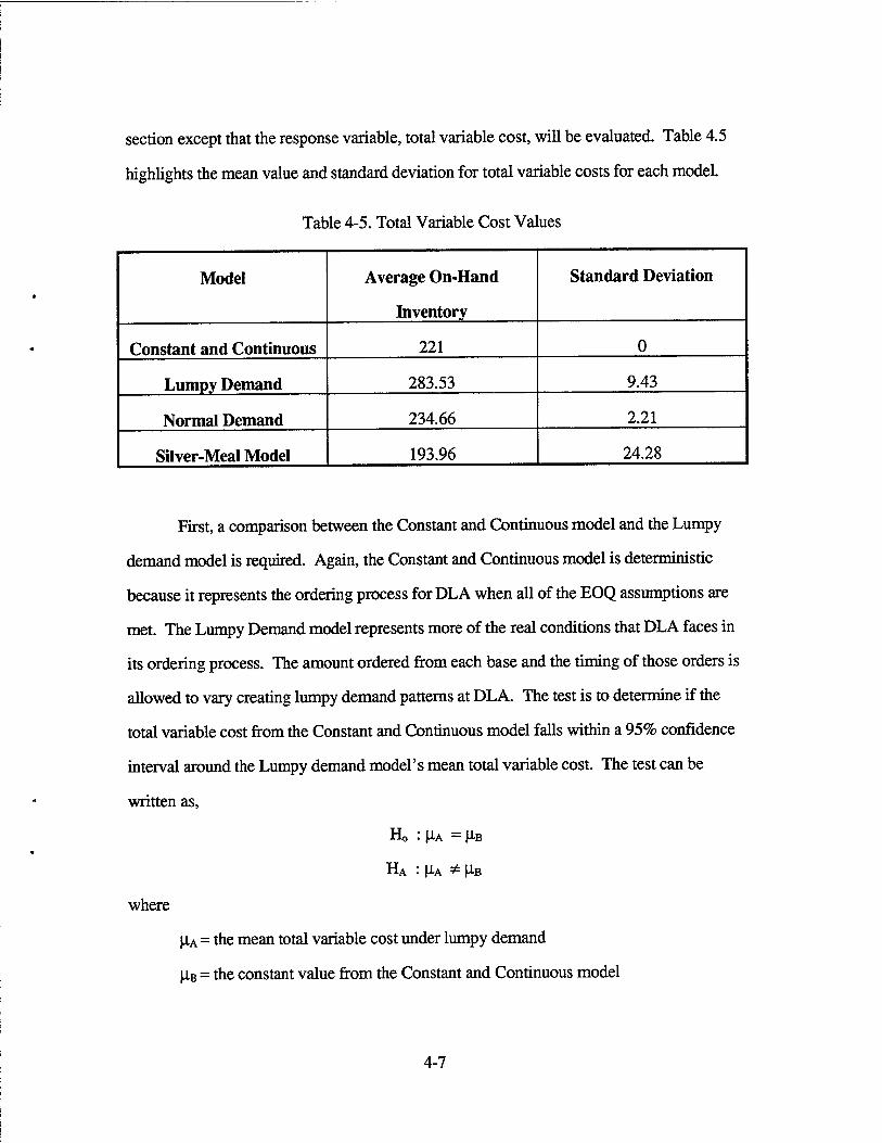
section except that the response variable, total variable cost, will be evaluated. Table 4.5

highlights the mean value and standard deviation for total variable costs for each model.

Table 4-5. Total Variable Cost Values

Model Average On-Hand

Inventory

Standard Deviation

Constant and Continuous 221 0

Lumpy Demand 283.53 9.43

Normal Demand 234.66 2.21

Silver-Meal Model 193.96 24.28

First, a comparison between the Constant and Continuous model and the Lumpy

demand model is required. Again, the Constant and Continuous model is deterministic

because it represents the ordering process for DLA when all of the EOQ assumptions are

met. The Lumpy Demand model represents more of the real conditions that DLA faces in

its ordering process. The amount ordered from each base and the timing of those orders is

allowed to vary creating lumpy demand patterns at DLA. The test is to determine if the

total variable cost from the Constant and Continuous model falls within a 95% confidence

interval around the Lumpy demand model's mean total variable cost. The test can be

written as,

Ho : |IA = M«

HA : UA *■ HB

where

HA = the mean total variable cost under lumpy demand

|HB = the constant value from the Constant and Continuous model

4-7

Table 4-6 shows the results of the test.

Table 4-6. Test of Hypothesis C&C vs. Lumpy

Lumpy demand with the

EOQ

Constant and Continuous

Demand

Variable Total Variable Cost Total Variable Cost

Mean Value 283.53 221

Upper 95% C.I. 287.05

Lower 95 % C.I. 280.01

As one can see from the table, the constant and continuous mean value is less than

the lower 95% bound and consequently does not lie within the 95% confidence interval.

Therefore, the null hypothesis that the two means are equal is rejected and the conclusion

reached is that lumpy demand conditions cause higher total variable costs to be incurred at

DLA if the present model is used.

The next step is to compare the lumpy demand model to the normal model. Here,

the amount bases order is allowed to fluctuate according to a normal distribution, which is

an assumption made in most inventory text books when describing continuous demand

patterns and also when calculating safety stock levels (Tersine, 1994:212). The test can

be written as,

Ho : (IA = M-B

HA : ^A * M-B

where,

|IA= the mean total variable cost under lumpy demand

4-8

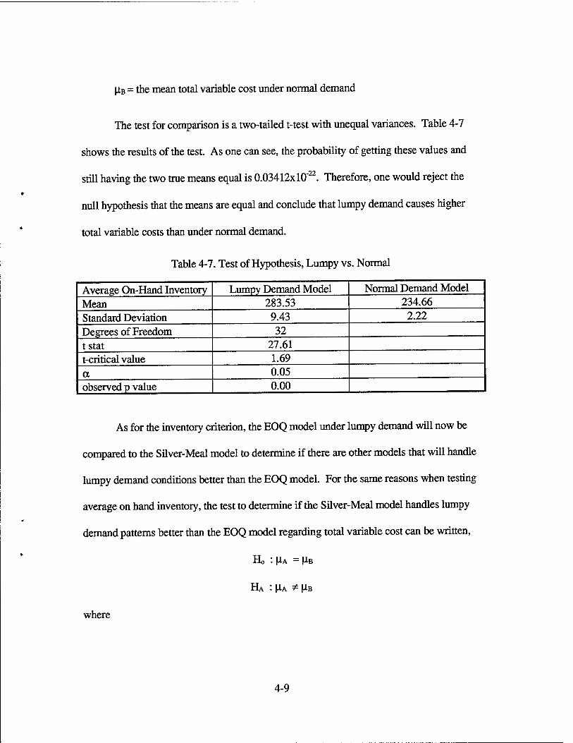
|iB = the mean total variable cost under normal demand

The test for comparison is a two-tailed t-test with unequal variances. Table 4-7

shows the results of the test. As one can see, the probability of getting these values and

still having the two true means equal is 0.03412xl0"22. Therefore, one would reject the

null hypothesis that the means are equal and conclude that lumpy demand causes higher

total variable costs than under normal demand.

Table 4-7. Test of Hypothesis, Lumpy vs. Normal

Average On-Hand Inventory Lumpy Demand Model Normal Demand Model

Mean 283.53 234.66

Standard Deviation 9.43 2.22

Degrees of Freedom 32 tstat 27.61 t-critical value 1.69 a 0.05 observed p value 0.00

As for the inventory criterion, the EOQ model under lumpy demand will now be

compared to the Silver-Meal model to determine if there are other models that will handle

lumpy demand conditions better than the EOQ model. For the same reasons when testing

average on hand inventory, the test to determine if the Silver-Meal model handles lumpy

demand patterns better than the EOQ model regarding total variable cost can be written,

Ho : |J.A = I^B

HA : |IA ^ |^B

where

4-9

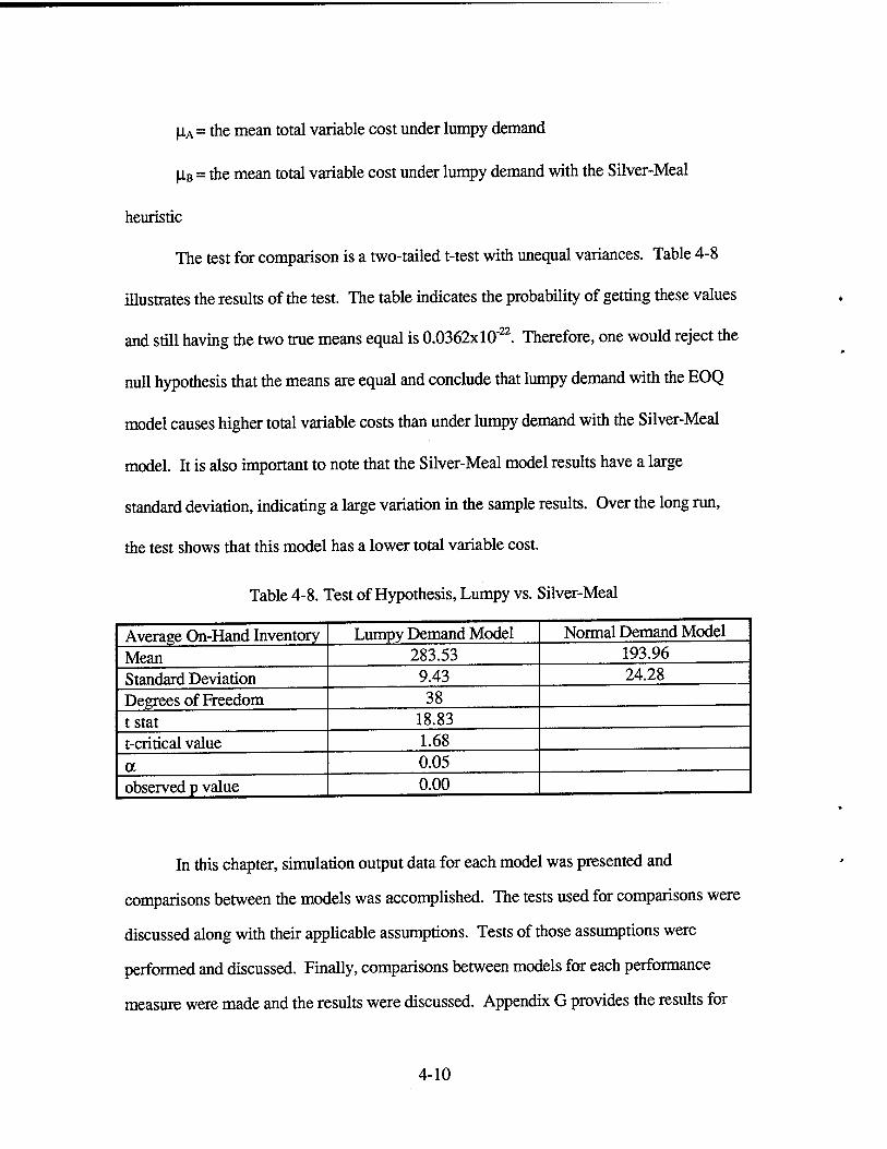
fiA = the mean total variable cost under lumpy demand

[IB = the mean total variable cost under lumpy demand with the Silver-Meal

heuristic

The test for comparison is a two-tailed t-test with unequal variances. Table 4-8

illustrates the results of the test. The table indicates the probability of getting these values

and still having the two true means equal is 0.0362xl0"22. Therefore, one would reject the

null hypothesis that the means are equal and conclude that lumpy demand with the EOQ

model causes higher total variable costs than under lumpy demand with the Silver-Meal

model. It is also important to note that the Silver-Meal model results have a large

standard deviation, indicating a large variation in the sample results. Over the long run,

the test shows that this model has a lower total variable cost.

Table 4-8. Test of Hypothesis, Lumpy vs. Silver-Meal

Average On-Hand Inventory Lumpy Demand Model Normal Demand Model Mean 283.53 193.96 Standard Deviation 9.43 24.28 Degrees of Freedom 38 tstat 18.83 t-critieal value 1.68 a 0.05 observed p value 0.00

In this chapter, simulation output data for each model was presented and

comparisons between the models was accomplished. The tests used for comparisons were

discussed along with their applicable assumptions. Tests of those assumptions were

performed and discussed. Finally, comparisons between models for each performance

measure were made and the results were discussed. Appendix G provides the results for

4-10

each run for every model and a detailed analysis of the comparisons. Now that the

experiment has been accomplished and the results presented, what should be done to

counter act lumpy demand conditions? Chapter V provides an explanation of the

conclusions from this research, some implications for DLA, and recommendations for

future research.

4-11

V. Conclusions. Implications and Recommendations

Based on the results of the experiment provided in Chapter IV, this chapter

provides implications about the appropriateness of the Defense Logistics Agency's

requirements model under lumpy demand conditions. From these conclusions,

management implications are drawn that DLA should consider given the lumpy nature of

the demand pattern they face. In addition, several recommendations for future research

are provided.

Conclusions

This section answers the research questions posed in Chapter I. The first question

to be answered is:

How does lumpy demand effect DIA's requirements model in regard to inventory levels

maintained at DLA?

The results presented in Chapter IV and in Appendix G provide several findings

with regard to average on-hand inventory. First, it is apparent that relaxing the

assumption of constant and continuous demand causes higher inventory levels to be

maintained at DLA. As one moves from the Constant and Continuous model to the

Normal model and finally, to the Lumpy model, total average on-hand inventory increases

dramatically. It is apparent that lumpy demand conditions cause the EOQ model to

maintain a higher amount of inventory even when the annual demand does not change.

5-1

From this, one can see that the requirements model used by DLA is not robust enough to

handle lumpy demand patterns.

The second research question is:

How does lumpy demand affect the total variable cost portion of DLA's requirements

model?

Based on the results of the experiment, it was discovered that lumpy demand

impacts total variable cost in a similar way as the average on hand inventory level. First,

relaxing the assumption of constant and continuous demand causes higher total variable

costs to be incurred. As one moves from the constant and continuous model to the

normal model and finally, to the lumpy model, total variable costs increase dramatically as

demand patterns approach the DLA environment. Therefore, it is apparent that the

requirements model used by DLA is not robust enough to handle lumpy demand patterns.

As mentioned earlier in Chapters IE and IV, this lumpy demand pattern is exactly what

DLA faces from Air Forces bases.

The third research question is:

Can a different approach provide improvement over the existing DLA model?

Given these conditions, a case could be made that DLA's requirements model

handles lumpy demand as well as any other model available. In order to test that

assertion, the Silver-Meal heuristic model was analyzed under the same lumpy

environment as the requirements model had undergone. The Silver-Meal heuristic model

was chosen for several reasons, its simplicity, its similarity to the EOQ model, and its

ability to handle lumpy demand patterns. Based on the results in Chapter IV, it is apparent

5-2

that the Silver-Meal model is able to provide lower average inventory levels and

ultimately, lower total variable costs than the current EOQ model, given lumpy demand

conditions. This also illustrates that there are other models in existence that do a much

better job of handling lumpy demand patterns than the EOQ model.

Implications

The conclusions have several implications for DLA and other organizations

operating in a multi-echelon environment. DLA inherently operates in a lumpy

environment. The two echelon system with EOQ models operating at both levels will

generate lumpy demand at the second echelon because of the EOQ ordering scheme at the

first level. This research has shown that lumpy demand adversely affects the average

inventory and total variable cost when an EOQ type requirements model is used at the

second echelon. The test of the Silver-Meal model illustrates that there are other models

available better suited for the lumpy demand conditions DLA faces. Given these results,

DLA should explore using another lot-sizing technique that would be more suited to

handling lumpy demand patterns.

Another consideration is forecasting methods and safety stock. This study

replicated the current forecasting technique being employed by DLA. However,

forecasting only affects the accuracy of demand estimates, as such it would not change the

demand pattern. This leaves a discussion of safety stock. Again, no safety stock was

utilized in this experiment; however, DLA does carry safety stock, as do the bases. These

stocks are used to maintain a certain customer service level. Again, these additional levels

of safety stock were not used in this experiment because they would compound the effects

5-3

of the variables evaluated. As such, the effect on the models of varying service levels was

not evaluated.

Recommendations for Future Research

There are several recommendations for future research that were identified

throughout this research.

1. Other inventory management models should be tested to determine the

appropriate model for DLA given their lumpy demand patterns. For example, the

Distribution Requirements Planning model appears to be well suited for DLA and its

environment. Due to the data sample distributions and assumptions of the statistical

analysis tools a similar experiment to this one is recommended to evaluate these alternative

models. A simulation of the model and operating environment could also be used to

compare the models in a lumpy demand environment. This research has shown that the

EOQ model is adversely affected by lumpy demand, therefore determining the optimal

model to use under these conditions would be of significance to DLA and the Air Force.

2. Another area of interest for research would be to quantify the overall effects of

lumpy demand on the Air Force. One approach would be to actually observe base level

ordering requirements and monitor them through the requisition process. Variables to

consider would be the ordering costs for the bases and DLA as well as the impact of

delivery delays at base level if stock outages occur. Another possible variable would be

the interaction with other services that are users of common items. An alternative

approach to analyzing the requisitioning of consumable items would be to apply the

5-4

findings of this study to a wartime scenario and track the consumable requisition through

the established supply channels as identified in Operations Plans for that particular theater.

A research goal could be to identify the best system for Air Force units to follow in the

deployed environment.

3. Another possible research avenue would be to test and determine the a better

forecasting method for the EOQ model given the lumpy demand patterns DLA faces. The

research should consider the time period being forecasted for as well as the forecasting

method. The current method, Double Exponential Smoothing, used by DLA was

employed in this experiment. However, there are other time series and explanatory

quantitative methods available that might produce better results. Examples of these

methods are Naive methods, other Smoothing methods, and Monitoring approaches that

could be effectively implemented in the DLA requirements model (Makridakis and

Wheelwright, 1989:14).

This study has discussed the appropriateness of the Defense Logistics Agency's

requirements model in managing consumable support for Air Force peculiar items.

Chapter I outlined the research problem and identified the operating environment in which

the EOQ model is used. Chapter II provided a thorough literature review of relevant

topics as well as recent research that dealt with lumpy demand. Chapter IE presented the

actual experiment methodology used in this research as well as verification and validation

of the simulation models used in this experiment. Chapter IV presented the results of the

experiments and discussed the statistical elements used to analyze the data. Chapter V

concluded the research by answering the research questions posed in chapter one and

5-5

raising additional questions worthy of further research. Overall, this research has

conclusively shown that lumpy demand adversely impacts both average on hand inventory

and total variable cost. Based on the sample data collected for this study, it is obvious

that DLA faces lumpy demand patterns from its customers, at least for Air Force specific

items. Yet, DLA uses a EOQ model which assumes that the demand patterns are constant

and continuous. This study has shown that the EOQ model does not handle lumpy

demand well and that there are other models available that can do a better job of managing

inventory levels in a lumpy demand environment.

5-6

References

APICS Dictionary. American Production and Inventory Control Society Dictionary (Seventh Edition). Falls Church VA: The Society. 1992.

Balwally, Nandakumar M. Operations Research Analysis and Projects Division, Defense Electronics Supply Center (DESC/EIR), Dayton OH. Telephone Interview. 12 December 1994.

Bilikan, Robert. Operations Research Analysis and Projects Division, Defense Electronics Supply Center (DESC/EIR), Dayton OH. Telephone Interview. 12 December 1994.

Blazer, Douglas J. "Variability of Demand: Why the Part is Never on the Shelf", Air Force Journal of Logistics. 11-22 (Spring,1985).

Choi, Richard H., Eric M. Malstrom, and Russell D. Tsai. "Evaluating Lot-sizing Methods in Multilevel Inventory Systems by Simulation," Production and Inventory Management Journal. 4-10 (Fourth Quarter, 1988).

Clark, Andrew J. "A Multiechelon, Dynamic Inventory Model," Naval Logistics Quarterly. 429-445 (Second Quarter, 1993).

Cooper, Donald E. and William Emory. Business Research Methods (Fifth Edition). Chicago: Irwin Incorporated, 1995.

Coyle, John J., Edward J. Bardi and C. John Langley, Jr. The Management of Business Logistics (Fifth Edition). New York: The West Publishing Company, 1988.

Defense Logistics Agency, Document DL107-2/11/91,2-1.

Delugio, Stephen A. and Carl D. Bhane. "Integrating Forecasts and Inventory Management of Low Volume Demands", 34th International Conference Proceedings. American Production and Inventory Control Society. Seattle: PAIM Press, 1991.

Harding, Michael. "Why Manage Inventory?" American Production and Inventory Control Society. 33rd International Conference Procedings, Vol: 42-247, (Oct 1990).

REF-1

Hood, William C. A Handbook of Supply Inventory Models. MS Thesis, AHT/GLM/LSMA/87S-35. School of Systems and Logistics, Air Force Institute of Technoloy (AU), Wright-Patterson AFB OH, September 1987 (AD-Al87269)

Knowles, Thomas W. Management Science. Building and Using Models Ilinois: Irwin Incorporated, 1989.

Law, Averill M. and W. David Kelton. Simulation Modeling and Analysis (Second Edition). New York: McGraw-Hill Incorporated, 1991.

Long, William S. and Douglas H. Engberson, The Effect of Violations of the Constant Demand Assumption on the Defense Logistic Agency Requirements Model. MS Thesis, AFIT/GLM/LAL/94S-15. School of Systems and Logistics, Air Force Institute of Technoloy (AU), Wright-Patterson AFB OH, September 1994 (AD-A285272).

McClave, James T. and P. George Benson. Statistics for Business and Economics (Sixth Edition). New York: Macmillen College Publishing Company, 1994.

Miller, George J. CPIM, "Inventory Reduction," American Production and Inventory Control Society. 33rd International Conference Procedings. Vol:242-247, (Oct 1990).

Madsen, Richard W., and Melvin L. Moeschberger. Statistical Concepts With Applications to Business and Economics. Prentice-Hall, Incorporated, New Jersey, 1980.

Makridakis, Spyros and Wheelwright, Steven C. Forecasting Methods for Management (Fifth Edition). New York: John Wiley & Sons, 1989.

Montgomery, Douglas C. Design and Analysis of Experiments (Third Edition). New York: John Wiley & Sons, 1991.

Peterson, Rein and Edward A. Silver. Decision Systems For Inventory Management and Production Planning. New York: John Wiley & Sons, 1979.

Prichard, James W. and Robert H. Eagle, Modern Inventory Management. New York: John Wiley & Sons, 1965.

Pritsker, Alan B. Introduction to Simulation and SLAM U (Third Edition). New York: Systems Publishing Corporation, 1986.

REF-2

Robinson, Nathaniel. The Defense Logistics Agency, Providing Logistics Support Throughout the Department of Defense. Research Report No. AU-ARI-92-4. Maxwell Air Force Base AL. Air University Press, October 1993.

Shields, Mathew D. "Economic Order Quantity and the Air Force." PhD Course Essay. The Ohio State University, Columbus OH, 1990.

Siegel, Joan. Statistix, Version 4.0. Tallahassee: Analytical Software, 1992.

Silver, Edward A. and Rein Peterson. Decision Systems for Inventory Management and Production Planning (2nd Edition). New York: John Wiley and Sons, 1985. 237-238.

Tersine, Richard J. Principles of Inventory and Materials Management (4th Edition). New Jersey: PTR Prentice Hall, 1994.

REF-3

ADDendix A. Samole Data

Sample data set, quarterly demand data periods 1-7.

Table A-1. Sample Data

*

NSN Q1 Q2 Q3 Q4 Q5 Q6 Q7 1260010735896 16 7 42 16 6 45 15 1440005727648 542 577 965 928 442 251 429 5805001408643 480 316 215 249 460 200 328 5805010773349 54 261 15 48 11 35 73 5805011775421 4927 10325 7680 6377 4299 8745 6414

5815006517030 691 289 352 475 52 13 23 5815009781363 1592 1855 2031 1474 1083 2464 1137 5895004375925 4 5 5 3 0 3 3 5895011706715 4 1 5 3 2 0 5 5905000037717 83 104 47 62 4 379 466 5905000069064 1 5 2 0 0 1 0 5905000514631 27 14 6 42 8 25 7 5905001048353 352 510 215 275 610 375 145 5905001114840 56 170 280 300 60 163 310 5905001193503 1838 3105 1208 2234 3055 3305 1937 5905001383431 2 2 3 6 1 0 101 5905001405657 76 114 164 78 72 638 536

r

A-l

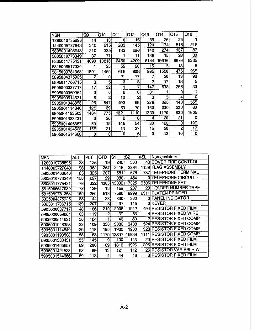
NSN Q9 Q10 Q11 Q12 Q13 Q14 Q15 Q16

1260010735896 14 13 0 15 38 26 25 1

1440005727648 340 215 283 145 120 134 518 216

5805001408643 210 225j 183 286 140 274 137 87

5805010773349 37 71 1 11 136 15 28 30

5805011775421 4690 10813 3450 4209 6144 19916 6679 8332

5815006517030 1 25 55 20 15 5 13 5

5815009781363 1801 1460 616 808 995 1550 476 265

5895004375925 2 0 21 77 7 20 13 98

5895011706715 3 5 3 3 2 17 18 2

5905000037717 17 32 1 7 147 538 266 30

5905000069064 0 0 0 0 31 1 0 1

5905000514631 6 2 12 2 3 5 4 0

5905001048353 25 547 493 95 276 390 143 555

5905001114840 125 39 53 70 150 230 230 60

5905001193503 1464 775 1321 1110 1330 1170 930 1605

5905001383431 0 20 2 0 4 20 21 0

5905001405657 60 15 145 54 30 123 0 199

5905001424523 155 21 13 27 15 20 2 17

5905001514666 0 0 0 5 0 13 10 0

NSN ALT PLT QFD S1 S2 VSL Nomenclature

1260010735896 83 125 19 245 303 43 COVER FIRE CONTROL

1440005727648 98 362 257 2415 2264 1139 FLAG ASSEMBLY

5805001408643 85 325 207 681 675 787 TELEPHONE TERMINAL

5805010773349 150 227 29 386 484 0 TELEPHONE CIRCUIT T

5805011775421 78 332 4305 15839 17325 9596 TELEPHONE SET

5815006517030 72 129 13 169 207 29 HOLDER NUMBER TAPE

5815009781363 150 260 513 7566 9999 2311 PLATEN PRINTER

5895004375925 88 44 33 330 330 0 PANEL INDICATOR

5895011706715 139 207 8 97 115 0 KEYER 5905000037717 48 166 210 2006 1912 494 RESISTOR FIXED FILM 5905000069064 63 119 2 39 63 4 RESISTOR FIXED WIRE

5905000514631 30 184 1 46 80 2 RESISTOR FIXED COMP

5905001048353 33 109 336 3386 3408 524 RESISTOR FIXED COMP

5905001114840 39 118 190 1900 1900 328 RESISTOR FIXED COMP

5905001193503 58 68 1179 13891 15989 1111 RESISTOR FIXED COMP

5905001383431 55 145 9 100 113 20 RESISTOR FIXED FILM

5905001405657 69 206 69 1310 1926 208 RESISTOR FIXED FILM

5905001424523 92 89 13 121 112 26 RESISTOR VARIABLE W

5905001514666 69 118 4 44 46 8 RESISTOR FIXED FILM

A-2

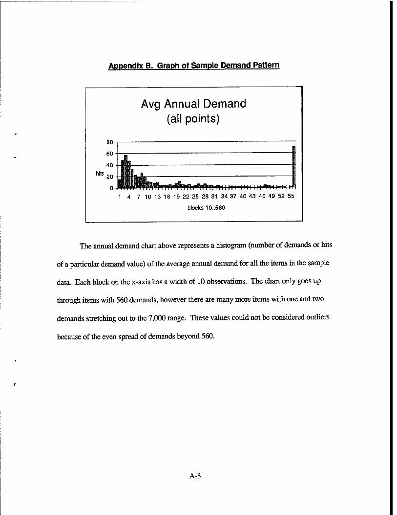
Appendix B. Graph of Sample Demand Pattern

Avg Annual Demand (all points)

1 4 7 10 13 16 19 22 25 28 31 34 37 40 43 46 49 52 55

blocks 10..560

The annual demand chart above represents a histogram (number of demands or hits

of a particular demand value) of the average annual demand for all the items in the sample

data. Each block on the x-axis has a width of 10 observations. The chart only goes up

through items with 560 demands, however there are many more items with one and two

demands stretching out to the 7,000 range. These values could not be considered outliers

because of the even spread of demands beyond 560.

A-3

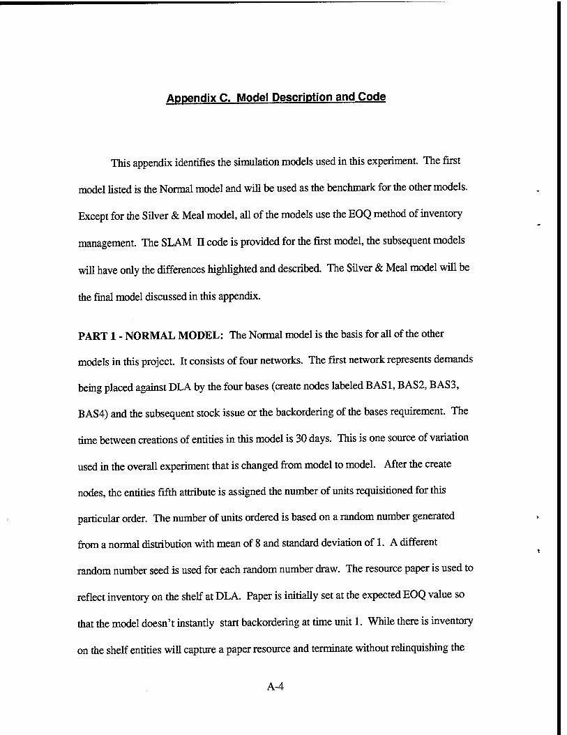
Appendix C. Model Description and Code

This appendix identifies the simulation models used in this experiment. The first

model listed is the Normal model and will be used as the benchmark for the other models.

Except for the Silver & Meal model, all of the models use the EOQ method of inventory

management. The SLAM II code is provided for the first model, the subsequent models

will have only the differences highlighted and described. The Silver & Meal model will be

the final model discussed in this appendix.

PART 1 - NORMAL MODEL: The Normal model is the basis for all of the other

models in this project. It consists of four networks. The first network represents demands

being placed against DLA by the four bases (create nodes labeled BAS1, BAS2, BAS3,

BAS4) and the subsequent stock issue or the backordering of the bases requirement. The

time between creations of entities in this model is 30 days. This is one source of variation

used in the overall experiment that is changed from model to model. After the create

nodes, the entities fifth attribute is assigned the number of units requisitioned for this

particular order. The number of units ordered is based on a random number generated

from a normal distribution with mean of 8 and standard deviation of 1. A different

random number seed is used for each random number draw. The resource paper is used to

reflect inventory on the shelf at DLA. Paper is initially set at the expected EOQ value so

that the model doesn't instantly start backordering at time unit 1. While there is inventory

on the shelf entities will capture a paper resource and terminate without relinquishing the

A-4

resource. Otherwise entities wait for replenishment at an await node (labeled BO).

Counters are used to track on hand inventory as well as the number of backorders.

Remember, safety stock was intentionally left out of the model to measure the true effects

of the different demand patterns. Consequently this model allows partial shipments to the

bases to fill requisitions.

The second network represents the daily releveling process the DLA computer

system executes to see if an order should be placed. At a create node labeled REPL, one

entity is created at each time unit and tests the on hand inventory plus the pipeline

inventory against the reorder point. If a requisition is required the cumulative order

counter is incremented and an order for the current EOQ is placed. This entity delays for

the lead time then increments the on hand inventory counter and alters the resource by

adding the EOQ. The alter allows backordered requisitions from the bases to be

processed and filled. If no requisition is required then a snapshot of on hand inventory is

captured to be used later in the model. Entities along both paths are routed through

collect nodes to generate statistical data.

The third network in this system calculates a new EOQ on a quarterly basis. Only

one entity is generated and cycles through this network continuously as long as the model

is running. Here the double exponential smoothing values are calculated and the quarterly

forecast demand is also derived in several steps. Next, user written FORTRAN functions

are invoked to complete the calculation of a reorder point and EOQ values. Now the

entity loops back to start the process over again but only after a 91 day delay.

A-5

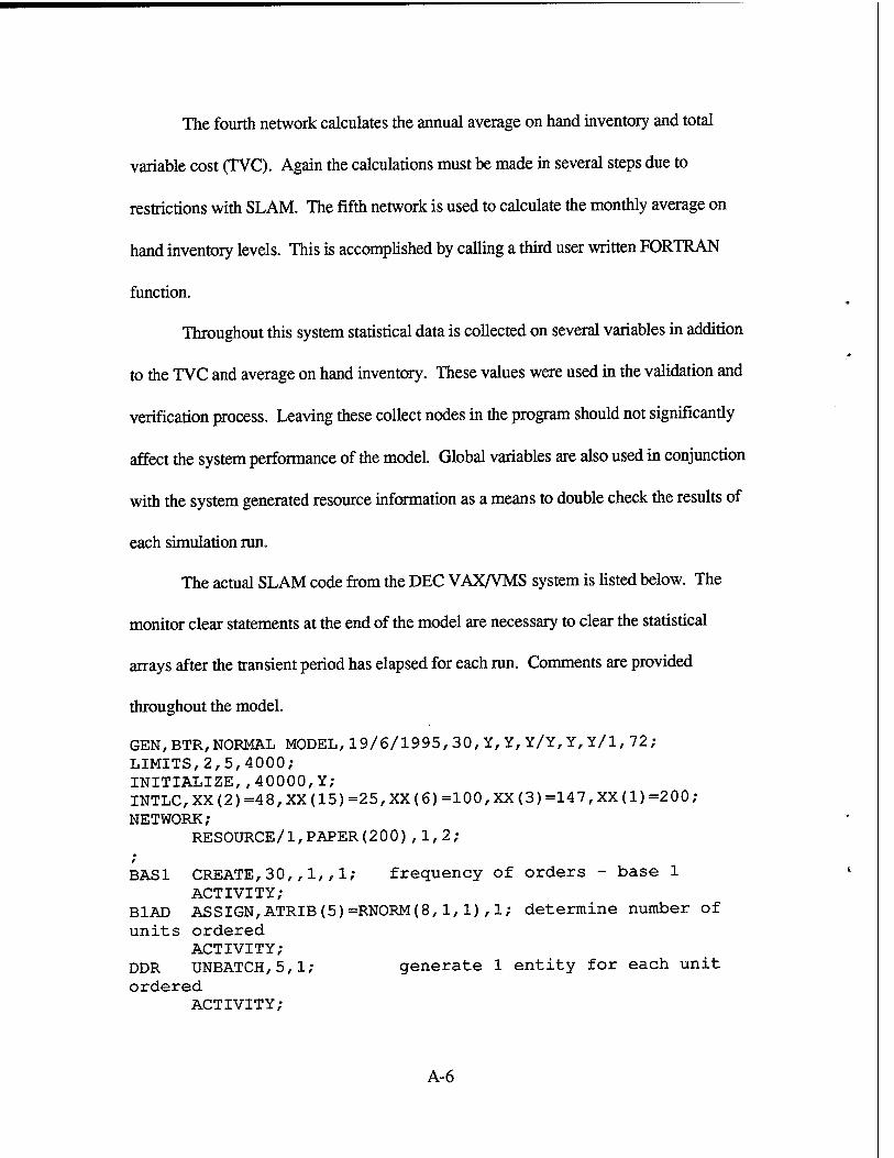
The fourth network calculates the annual average on hand inventory and total

variable cost (TVC). Again the calculations must be made in several steps due to

restrictions with SLAM. The fifth network is used to calculate the monthly average on

hand inventory levels. This is accomplished by calling a third user written FORTRAN

function.

Throughout this system statistical data is collected on several variables in addition

to the TVC and average on hand inventory. These values were used in the validation and

verification process. Leaving these collect nodes in the program should not significantly

affect the system performance of the model. Global variables are also used in conjunction

with the system generated resource information as a means to double check the results of

each simulation run.

The actual SLAM code from the DEC VAX/VMS system is listed below. The

monitor clear statements at the end of the model are necessary to clear the statistical

arrays after the transient period has elapsed for each run. Comments are provided

throughout the model.

GEN,BTR,NORMAL MODEL,19/6/1995,30,Y,Y,Y/Y,Y,Y/l,72; LIMITS,2,5,4000; INITIALIZE,,40000,Y; INTLC,XX(2)=48,XX(15)=25,XX(6)=100,XX(3)=147,XX(1)=200; NETWORK;

RESOURCE/1,PAPER(200),1,2; r

BASl CREATE,30,,1,,1; frequency of orders - base 1 ACTIVITY;

B1AD ASSIGN,ATRIB(5)=RNORM(8,l,l),1; determine number of units ordered

ACTIVITY; DDR UNBATCH,5,1; generate 1 entity for each unit ordered

ACTIVITY;

A-6

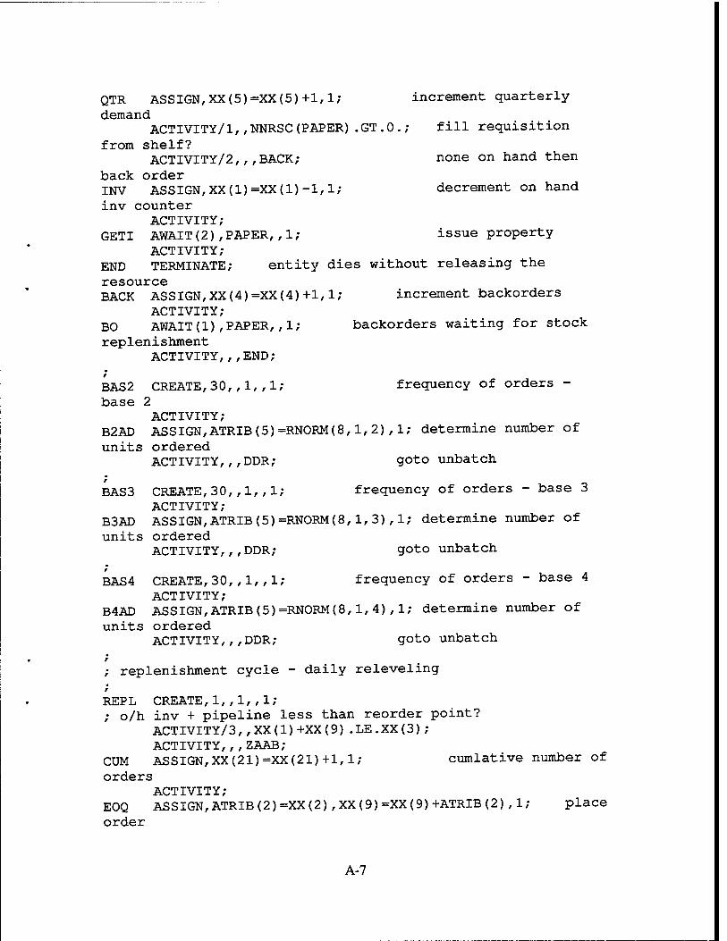
QTR ASSIGN,XX(5)=XX(5)+1,1; increment quarterly demand

ACTIVITY/1, ,NNRSC(PAPER) .GT.O.; fill requisition from shelf?

ACTIVITY/2,,,BACK; none on hand then back order INV ASSIGN,XX(1)=XX(1)-1,1; decrement on hand inv counter

ACTIVITY; GETI AWAIT(2),PAPER,,1; issue property

ACTIVITY; END TERMINATE; entity dies without releasing the resource BACK ASSIGN, XX(4)=XX(4)+1,1; increment backorders

ACTIVITY; BO AWAIT(1),PAPER,,1; backorders waiting for stock replenishment

ACTIVITY,,,END;

BAS2 CREATE, 30,, 1,,1; frequency of orders - base 2

ACTIVITY; B2AD ASSIGN,ATRIB(5)=RNORM(8,l,2),l; determine number of units ordered

ACTIVITY,,,DDR; gotounbatch

BAS3 CREATE, 30,, 1,,1; frequency of orders - base 3 ACTIVITY;

B3AD ASSIGN,ATRIB(5)=RNORM(8,l,3),1; determine number of units ordered

ACTIVITY,,,DDR; goto unbatch

BAS4 CREATE, 30,, 1,,1; frequency of orders - base 4 ACTIVITY;

B4AD ASSIGN,ATRIB(5)=RNORM(8,l,4),l; determine number of units ordered

ACTIVITY,,,DDR; gotounbatch

replenishment cycle - daily releveling

REPL CREATE, 1, , 1, ,1; ; o/h inv + pipeline less than reorder point?

ACTIVITY/3,, XX(1)+XX(9) .LE.XX(3); ACTIVITY, , , ZAAB;

CUM ASSIGN,XX(21)=XX(21)+1,1; cumlative number of orders

ACTIVITY; EOQ ASSIGN,ATRIB(2)=XX(2),XX(9)=XX(9)+ATRIB(2),1; place order

A-7

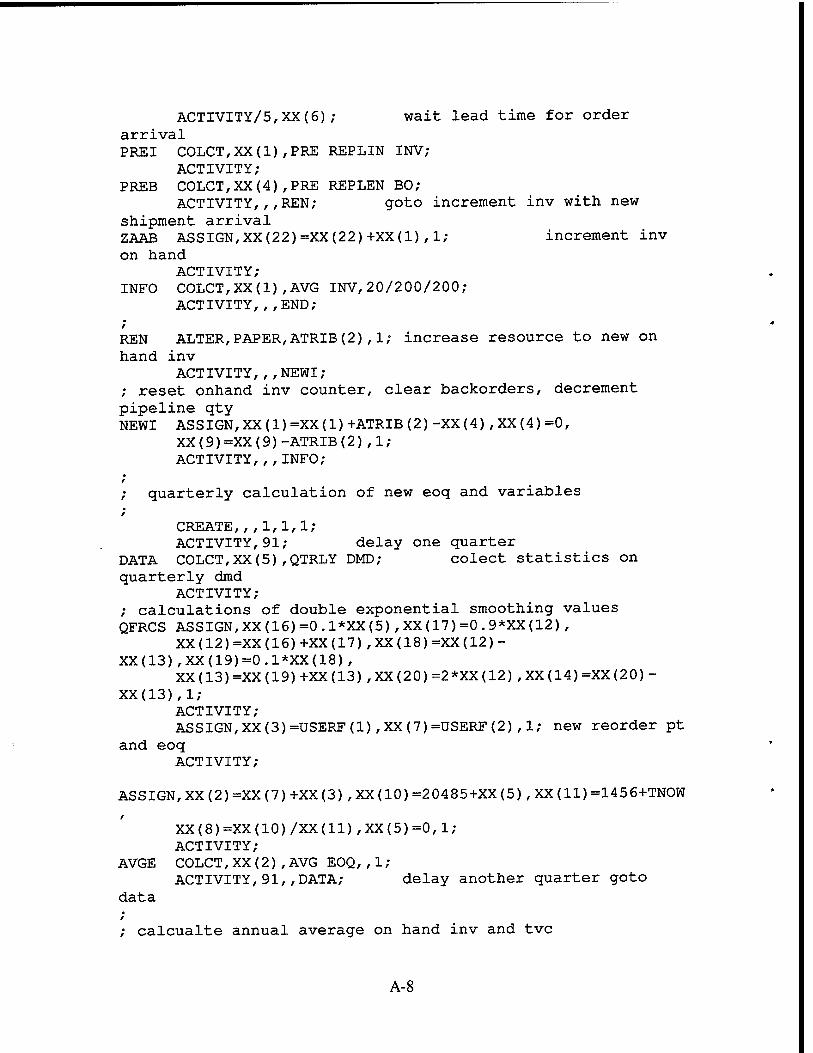
ACTIVITY/5,XX(6); wait lead time for order arrival PREI C0LCT,XX(1),PRE REPLIN INV;

ACTIVITY; PREB C0LCT,XX(4),PRE REPLEN BO;

ACTIVITY,,,REN; goto increment inv with new shipment arrival ZAAB ASSIGN,XX(22)=XX(22)+XX(1),1; increment inv on hand

ACTIVITY; INFO C0LCT,XX(1),AVG INV,20/200/200;

ACTIVITY,,,END;

REN ALTER,PAPER,ATRIB(2),1; increase resource to new on hand inv

ACTIVITY,,,NEWI; ; reset onhand inv counter, clear backorders, decrement pipeline qty NEWI ASSIGN,XX(1)=XX(1)+ATRIB(2)-XX(4) ,XX(4)=0,

XX(9)=XX(9)-ATRIB(2),1; ACTIVITY,,,INFO;

quarterly calculation of new eoq and variables

CREATE,, ,1,1,1; ACTIVITY,91; delay one quarter

DATA COLCT,XX(5),QTRLY DMD; colect statistics on quarterly dmd

ACTIVITY; ; calculations of double exponential smoothing values QFRCS ASSIGN,XX(16)=0.1*XX(5),XX(17)=0.9*XX(12),

XX(12)=XX(16)+XX(17),XX(18)=XX(12)- XX(13),XX(19)=0.1*XX(18),

XX(13)=XX(19)+XX(13) ,XX(20)=2*XX(12) ,XX(14) =XX(20)- XX (13) , IN-

ACTIVITY ; ASSIGN,XX(3)=USERF(1),XX(7)=USERF(2),1; new reorder pt

and eoq ACTIVITY;

ASSIGN, XX(2)=XX(7)+XX(3),XX(10)=20485+XX(5),XX(11)=1456+TNOW

XX(8)=XX(10)/XX(11),XX(5)=0,1; ACTIVITY;

AVGE COLCT,XX(2),AVG EOQ,,1; ACTIVITY, 91,,DATA; delay another quarter goto

data

; calcualte annual average on hand inv and tvc

A-8

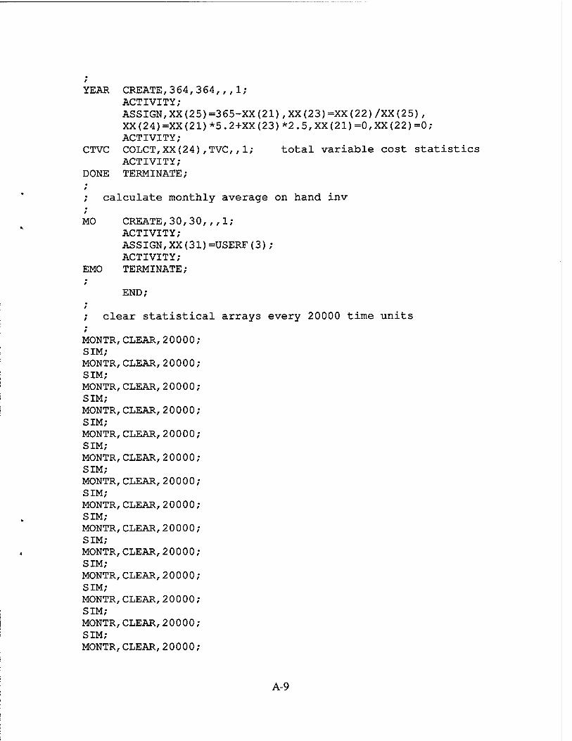
YEAR CREATE, 364, 364,, , IN- ACTIVITY ; ASSIGN,XX(25)=365-XX(21),XX(23)=XX(22)/XX(25), XX(24)=XX(21)*5.2+XX(23)*2.5,XX(21)=0,XX(22)=0; ACTIVITY;

CTVC COLCT,XX(24),TVC,, 1; total variable cost statistics ACTIVITY;

DONE TERMINATE;

calculate monthly average on hand inv

MO CREATE,30,30, , , 1; ACTIVITY; ASSIGN,XX(31)=USERF(3) ; ACTIVITY;

EMO TERMINATE;

END;

clear statistical arrays every 20000 time units

MONTR,CLEAR,20000 SIM; MONTR,CLEAR,20000 SIM; MONTR,CLEAR,20000 SIM; MONTR,CLEAR,20000 SIM; MONTR,CLEAR,20000 SIM; MONTR,CLEAR,20000 SIM; MONTR,CLEAR,20000 SIM; MONTR,CLEAR,20000 SIM; MONTR,CLEAR,20000 SIM; MONTR,CLEAR,20000 SIM; MONTR,CLEAR,20000 SIM; MONTR,CLEAR,20000 SIM; MONTR,CLEAR,20000 SIM; MONTR,CLEAR,20000

A-9

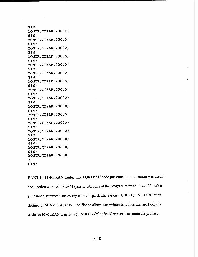
SIM; MONTR,CLEAR,20000 SIM; MONTR,CLEAR,20000 SIM; MONTR,CLEAR,20000 SIM; MONTR,CLEAR,20000 SIM; MONTR,CLEAR,20000 SIM; MONTR,CLEAR,20000 SIM; MONTR,CLEAR,20000 SIM; MONTR,CLEAR,20000 SIM; MONTR,CLEAR,20000 SIM; MONTR,CLEAR,20000 SIM; MONTR,CLEAR,20000 SIM; MONTR,CLEAR,20000 SIM; MONTR,CLEAR,20000 SIM; MONTR,CLEAR,20000 SIM; MONTR,CLEAR,20000 SIM; MONTR,CLEAR,20000 / FIN;

PART 2 - FORTRAN Code: The FORTRAN code presented in this section was used in

conjunction with each SLAM system. Portions of the program main and user-f function

are canned statements necessary with this particular system. USERF(IFN) is a function

defined by SLAM that can be modified to allow user written functions that are typically

easier in FORTRAN than in traditional SLAM code. Comments separate the primary

A-10

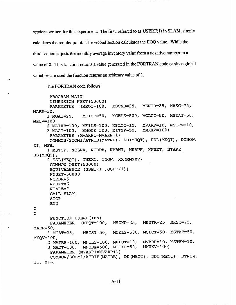
sections written for this experiment. The first, referred to as USERF(l) in SLAM, simply

calculates the reorder point. The second section calculates the EOQ value. While the

third section adjusts the monthly average inventory value from a negative number to a

value of 0. This function returns a value generated in the FORTRAN code or since global

variables are used the function returns an arbitrary value of 1.

The FORTRAN code follows.

PROGRAM MAIN DIMENSION NSET(50000) PARAMETER (MEQT=100, MSCND=25, MENTR=25, MRSC=75,

MARR=50, 1 MGAT=25, MHIST=50, MCELS=500, MCLCT=50, MSTAT=50,

MEQV=100, 2 MATRB=100, MFILS=100, MPLOT=10, MVARP=10, MSTRM=10, 3 MACT=100, MNODE=500, MITYP=50, MMXXV=100) PARAMETER (MVARP1=MVARP+1) COMMON/SCOMl/ATRIB(MATRB), DD(MEQT), DDL(MEQT), DTNOW,

II, MFA, 1 MSTOP, NCLNR, NCRDR, NPRNT, NNRUN, NNSET, NTAPE,

SS(MEQT), 2 SSL(MEQT), TNEXT, TNOW, XX(MMXXV) COMMON QSET(50000) EQUIVALENCE (NSET(1),QSET(1)) NNSET=50000 NCRDR=5 NPRNT=6 NTAPE=7 CALL SLAM STOP END

C C

FUNCTION USERF(IFN) PARAMETER (MEQT=100, MSCND=25, MENTR=25, MRSC=75,

MARR=50, 1 MGAT=25, MHIST=50, MCELS=500, MCLCT=50, MSTAT=50,

MEQV=100, 2 MATRB=100, MFILS=100, MPLOT=10, MVARP=10, MSTRM=10, 3 MACT=100, MNODE=500, MITYP=50, MMXXV=100) PARAMETER (MVARP1=MVARP+1) COMMON/SCOMl/ATRIB(MATRB), DD(MEQT), DDL(MEQT), DTNOW,

II, MFA,

A-ll

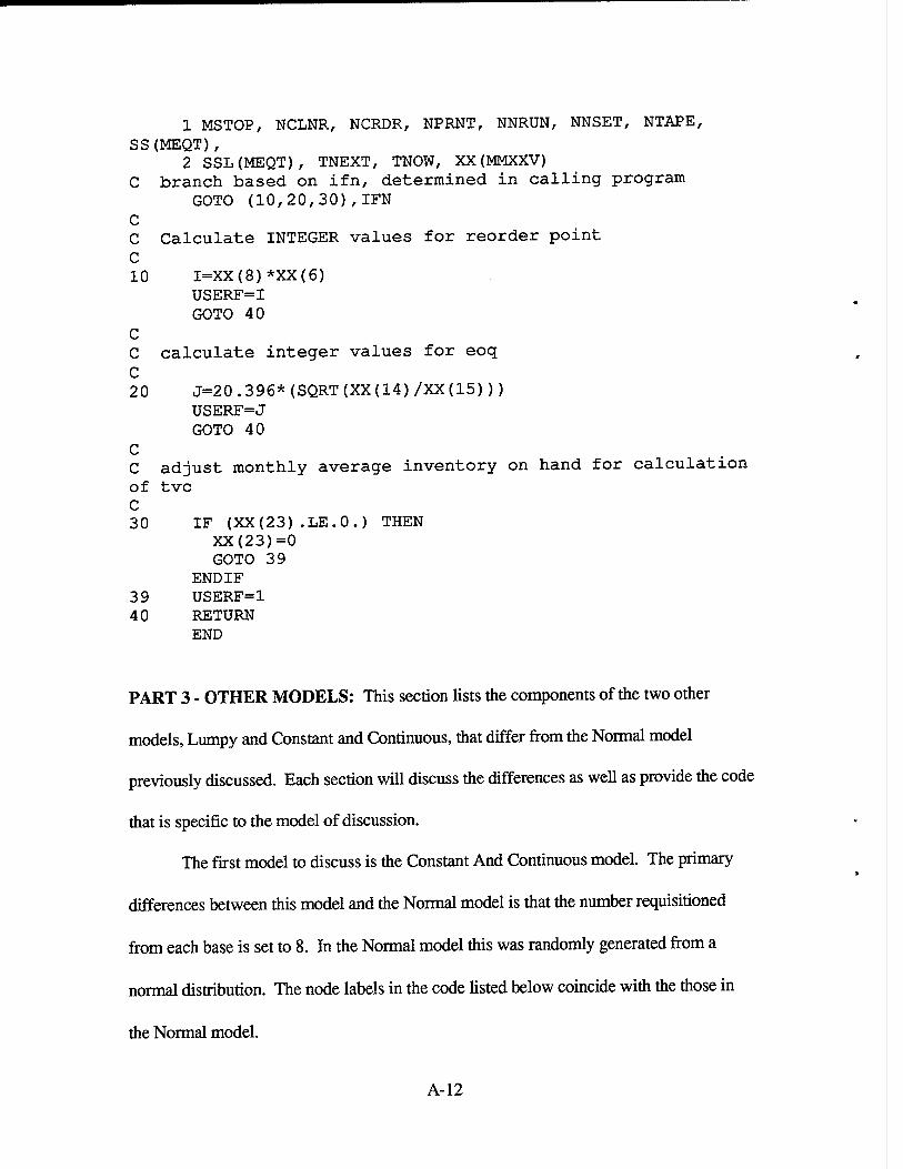
1 MSTOP, NCLNR, NCRDR, NPRNT, NNRUN, NNSET, NTAPE, SS(MEQT),

2 SSL(MEQT), TNEXT, TNOW, XX(MMXXV) C branch based on ifn, determined in calling program

GOTO (10,20,30),IFN C C Calculate INTEGER values for reorder point C 10 I=XX(8)*XX(6)

USERF=I GOTO 40

C C calculate integer values for eoq C 20 J=20.396*(SQRT(XX(14)/XX(15)))

USERF=J GOTO 40

C C adjust monthly average inventory on hand for calculation of tvc C 30 IF (XX(23).LE.0.) THEN

XX(23)=0 GOTO 39

END IF 39 USERF=1 40 RETURN

END

PART 3 - OTHER MODELS: This section lists the components of the two other

models, Lumpy and Constant and Continuous, that differ from the Normal model

previously discussed. Each section will discuss the differences as well as provide the code

that is specific to the model of discussion.

The first model to discuss is the Constant And Continuous model. The primary

differences between this model and the Normal model is that the number requisitioned

from each base is set to 8. In the Normal model this was randomly generated from a

normal distribution. The node labels in the code listed below coincide with the those in

the Normal model.

A-12

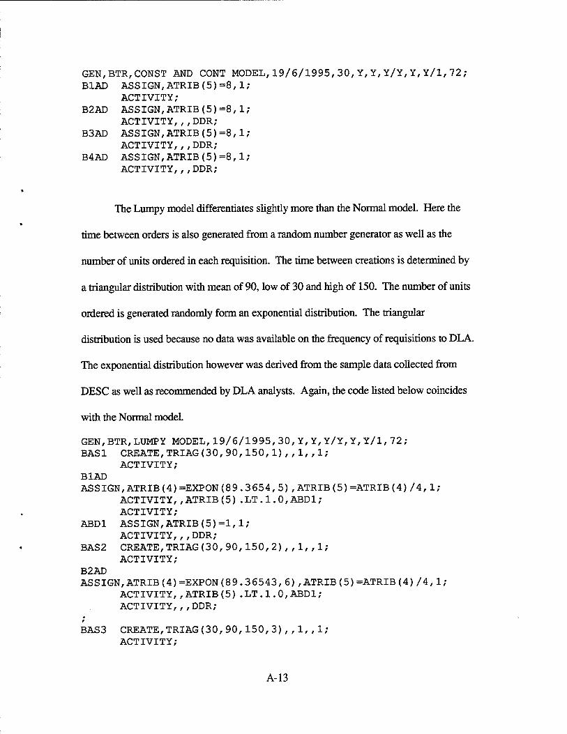
GEN,BTR,CONST AND CONT MODEL,19/6/1995,30,Y,Y,Y/Y,Y,Y/l,72; B1AD ASSIGN,ATRIB(5)=8,1,

ACTIVITY; B2AD ASSIGN,ATRIB(5)=8,1

ACTIVITY,,,DDR; B3AD ASSIGN,ATRIB(5)=8,1

ACTIVITY,,,DDR; B4AD ASSIGN,ATRIB(5)=8,1

ACTIVITY,,,DDR;

The Lumpy model differentiates slightly more than the Normal model. Here the

time between orders is also generated from a random number generator as well as the

number of units ordered in each requisition. The time between creations is determined by

a triangular distribution with mean of 90, low of 30 and high of 150. The number of units

ordered is generated randomly form an exponential distribution. The triangular

distribution is used because no data was available on the frequency of requisitions to DLA.

The exponential distribution however was derived from the sample data collected from

DESC as well as recommended by DLA analysts. Again, the code listed below coincides

with the Normal model.

GEN,BTR,LUMPY MODEL,19/6/1995,30,Y,Y,Y/Y,Y,Y/l,72; BAS1 CREATE, TRIAG (30, 90, 150,1), ,l/f IN-

ACTIVITY; B1AD ASSIGN,ATRIB(4)=EXPON(89.3654,5),ATRIB(5)=ATRIB(4)/4,1;

ACTIVITY,,ATRIB(5).LT.1.0,ABD1; ACTIVITY;

ABD1 ASSIGN,ATRIB(5)=1,1; ACTIVITY,,,DDR;

BAS2 CREATE, TRIAG (30, 90,150, 2) , ,1, , IN- ACTIVITY ;

B2AD ASSIGN,ATRIB(4)=EXPON(89.36543,6), ATRIB (5) =ATRIB (4)/4, 1;

ACTIVITY,,ATRIB(5).LT.1.0,ABD1; ACTIVITY, ,,DDR;

r

BAS3 CREATE,TRIAG(30,90,150,3),, 1,,1,- ACTIVITY;

A-13

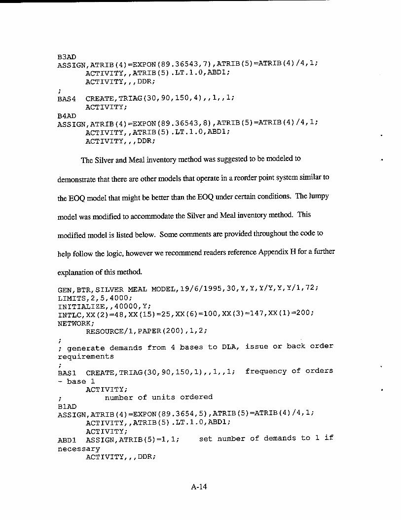
B3AD ASSIGN,ATRIB(4)=EXPON(89.36543,7),ATRIB(5)=ATRIB(4)/4,l;

ACTIVITY,,ATRIB(5).LT.1.0,ABD1; ACTIVITY,,,DDR;

BAS4 CREATE,TRIAG(30, 90,150, 4) , , 1, , 1; ACTIVITY;

B4AD ASSIGN,ATRIB(4)=EXPON(89.36543,8),ATRIB(5)=ATRIB(4)/4,l;

ACTIVITY,,ATRIB(5).LT.1.0,ABD1; ACTIVITY,,,DDR;

The Silver and Meal inventory method was suggested to be modeled to

demonstrate that there are other models that operate in a reorder point system similar to

the EOQ model that might be better than the EOQ under certain conditions. The lumpy

model was modified to accommodate the Silver and Meal inventory method. This

modified model is listed below. Some comments are provided throughout the code to

help follow the logic, however we recommend readers reference Appendix H for a further

explanation of this method.

GEN,BTR,SILVER MEAL MODEL,19/6/1995,30,Y,Y,Y/Y,Y,Y/l,72; LIMITS,2,5,4000; INITIALIZE,,40000,Y; INTLC,XX(2)=48,XX (15)=25,XX(6)=100,XX(3)=147,XX(1) =200;

NETWORK; RESOURCE/1,PAPER(200),1,2;

; generate demands from 4 bases to DLA, issue or back order requirements

BAS1 CREATE,TRIAG(30,90,150,1),,1,,1; frequency of orders - base 1

ACTIVITY; ; number of units ordered B1AD ASSIGN,ATRIB(4)=EXPON(89.3654,5),ATRIB(5)=ATRIB(4) /4, 1;

ACTIVITY,,ATRIB(5).LT.1.0,ABD1; ACTIVITY;

ABD1 ASSIGN,ATRIB(5)=1,1; set number of demands to 1 if necessary

ACTIVITY,,,DDR;

A-14

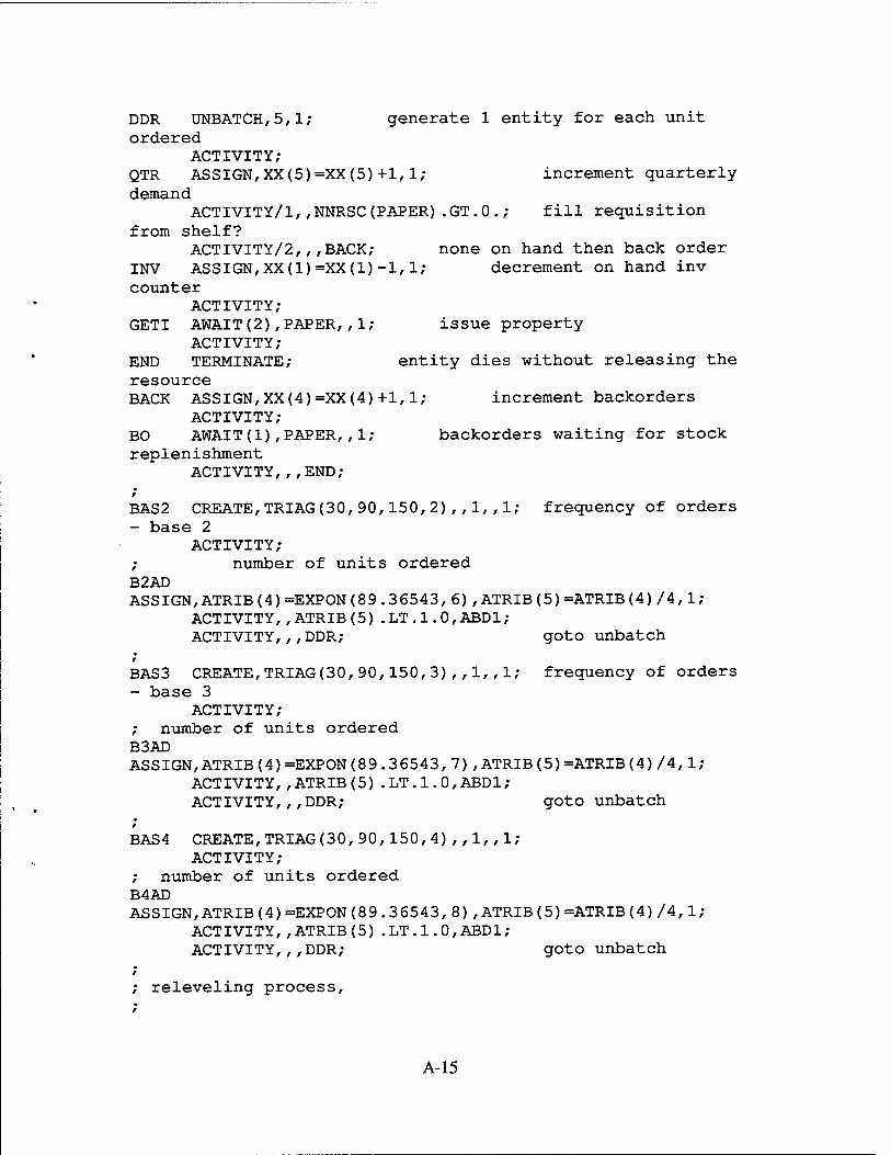
DDR UNBATCH,5,1; generate 1 entity for each unit ordered

ACTIVITY; QTR ASSIGN,XX(5)=XX(5)+1,1; increment quarterly demand

ACTIVITY/1,,NNRSC(PAPER).GT.O.; fill requisition from shelf?

ACTIVITY/2,,,BACK; none on hand then back order INV ASSIGN,XX(1)=XX(1)-1,1; decrement on hand inv counter

ACTIVITY; GETI AWAIT(2),PAPER,,1; issue property

ACTIVITY; END TERMINATE; entity dies without releasing the resource BACK ASSIGN,XX(4)=XX(4)+1,1; increment backorders

ACTIVITY; BO AWAIT(1),PAPER,,1; backorders waiting for stock replenishment

ACTIVITY,,,END; f

BAS2 CREATE,TRIAG(30,90,150,2),,1,,1; frequency of orders - base 2

ACTIVITY; ; number of units ordered B2AD ASSIGN,ATRIB(4)=EXPON(89.36543,6),ATRIB(5)=ATRIB(4)/4,l;

ACTIVITY, ,ATRIB (5) .LT . 1. 0, ABDIN- ACTIVITY, ,,DDR; goto unbatch

r

BAS3 CREATE,TRIAG(30,90,150,3),,1,,1; frequency of orders - base 3

ACTIVITY; ; number of units ordered B3AD ASSIGN,ATRIB(4)=EXPON(89.36543,7),ATRIB(5)=ATRIB(4)/4,l;

ACTIVITY,,ATRIB(5).LT.1.0,ABD1; ACTIVITY,,,DDR; goto unbatch

BAS4 CREATE,TRIAG(30,90,150,4), ,1,,1,- ACTIVITY;

; number of units ordered B4AD ASSIGN,ATRIB(4)=EXPON(89.36543, 8) , ATRIB (5)=ATRIB (4)/4, 1,-

ACTIVITY, , ATRIB (5) .LT.1.0,ABD1; ACTIVITY,,,DDR; goto unbatch

releveling process,

A-15

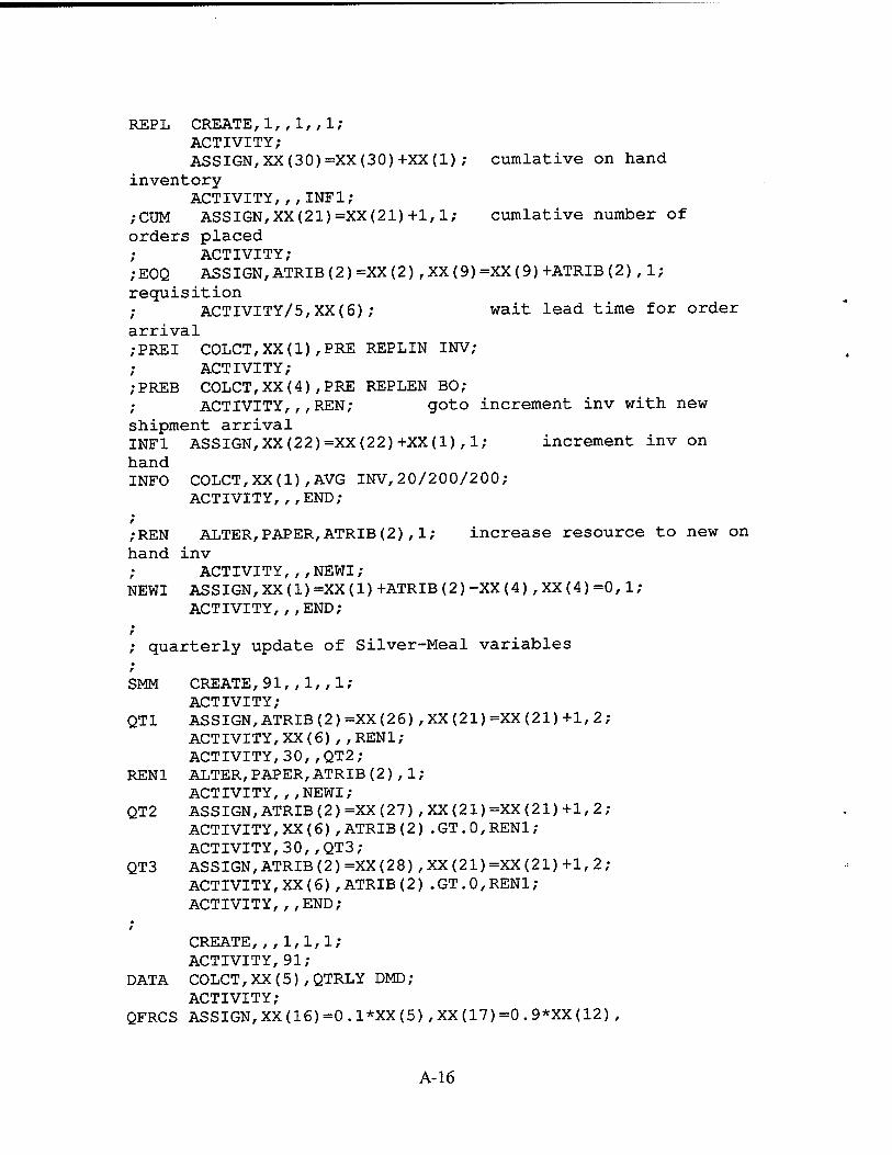
REPL CREATE,1,, 1,,1; ACTIVITY; ASSIGN,XX(30)=XX(30)+XX(1); cumlative on hand

inventory ACTIVITY,,,INF1;

;CUM ASSIGN,XX(21)=XX(21)+1,1; cumlative number of orders placed

ACTIVITY; ;EOQ ASSIGN,ATRIB(2)=XX(2),XX(9)=XX(9)+ATRIB(2),1; requisition

ACTIVITY/5,XX(6); wait lead time for order arrival PREI C0LCT,XX(1),PRE REPLIN INT-

ACT IVITY; PREB C0LCT,XX(4),PRE REPLEN BO;

ACTIVITY,,,REN; goto increment inv with new shipment arrival INF1 ASSIGN,XX(22)=XX(22)+XX(1),1; increment inv on hand INFO C0LCT,XX(1),AVG INV,20/200/200;

ACTIVITY,,,END;

;REN ALTER,PAPER,ATRIB(2),1; increase resource to new on hand inv

ACTIVITY,,,NEWI; NEWI ASSIGN, XX(1)=XX(1)+ATRIB(2)-XX(4) ,XX(4)=0, 1;

ACTIVITY,,,END;

quarterly update of Silver-Meal variables

SMM CREATE,91,,1, , 1; ACTIVITY;

QT1 ASSIGN,ATRIB(2)=XX(26),XX(21)=XX(21)+1,2; ACTIVITY,XX(6),,REN1; ACTIVITY,30,,QT2;

REN1 ALTER,PAPER,ATRIB(2),1; ACTIVITY,,,NEWI;

QT2 ASSIGN,ATRIB(2)=XX(27),XX(21)=XX(21)+1,2; ACTIVITY,XX(6),ATRIB(2).GT.0,REN1; ACTIVITY,30,, QT3;

QT3 ASSIGN,ATRIB(2)=XX(28),XX(21)=XX(21)+1,2; ACTIVITY,XX(6),ATRIB(2).GT.0,REN1; ACTIVITY,,,END;

CREATE, ,,1,1,1; ACTIVITY,91;

DATA COLCT,XX(5),QTRLY DMD; ACTIVITY;

QFRCS ASSIGN,XX(16)=0.1*XX(5),XX(17)=0.9*XX(12),

A-16

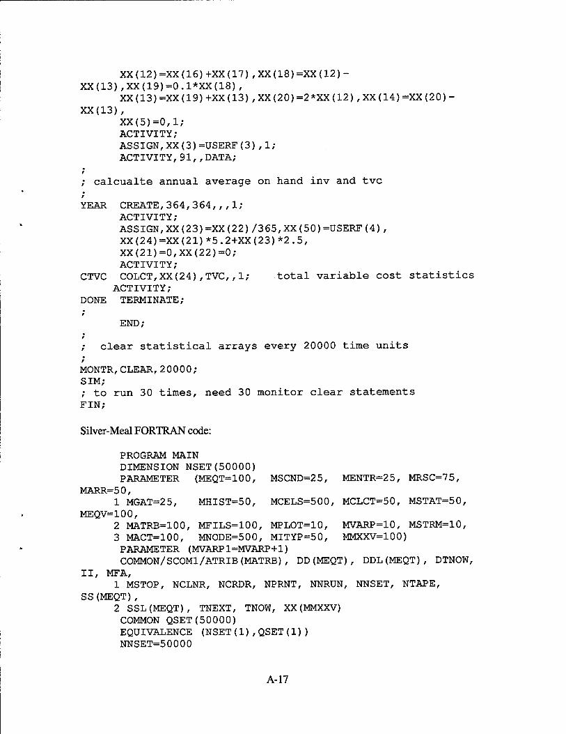
XX(12)=XX(16)+XX(17) ,XX(18)=XX(12)- XX(13) ,XX(19)=0.1*XX(18) ,

XX(13)=XX(19)+XX(13),XX(20)=2*XX(12),XX(14)=XX(20)- XX(13),

XX(5)=0,1; ACTIVITY; ASSIGN,XX(3)=USERF(3),1; ACTIVITY, 91, , DATA;

calcualte annual average on hand inv and tvc

YEAR CREATE,364,364,,,1; ACTIVITY; ASSIGN,XX(23)=XX(22)/365,XX(50)=USERF(4), XX(24)=XX(21)*5.2+XX(23)*2.5, XX(21)=0,XX(22)=0; ACTIVITY;

CTVC COLCT,XX(24),TVC,, 1; total variable cost statistics ACTIVITY;

DONE TERMINATE; r

END; r

clear statistical arrays every 20000 time units

MONTR,CLEAR,20000; SIM; ; to run 30 times, need 30 monitor clear statements FIN;

Silver-Meal FORTRAN code:

PROGRAM MAIN DIMENSION NSET(50000) PARAMETER (MEQT=100, MSCND=25, MENTR=25, MRSC=75,

MARR=50, 1 MGAT=25, MHIST=50, MCELS=500, MCLCT=50, MSTAT=50,

MEQV=100, 2 MATRB=100, MFILS=100, MPLOT=10, MVARP=10, MSTRM=10, 3 MACT=100, MNODE=500, MITYP=50, MMXXV=100) PARAMETER (MVARP1=MVARP+1) COMMON/SCOMl/ATRIB(MATRB), DD(MEQT), DDL(MEQT), DTNOW,

II, MFA, 1 MSTOP, NCLNR, NCRDR, NPRNT, NNRUN, NNSET, NTAPE,

SS(MEQT) , 2 SSL(MEQT), TNEXT, TNOW, XX(MMXXV) COMMON QSET(50000) EQUIVALENCE (NSET(1),QSET(1)) NNSET=50000

A-17

NCRDR=5 NPRNT=6 NTAPE=7 CALL SLAM STOP END

C C

FUNCTION USERF(IFN) PARAMETER (MEQT=100, MSCND=25, MENTR=25, MRSC=75,

MARR=50, 1 MGAT=25, MHIST=50, MCELS=500, MCLCT=50, MSTAT=50,

MEQV=100, 2 MATRB=100, MFILS=100, MPLOT=10, MVARP=10, MSTRM=10, 3 MACT=100, MNODE=500, MITYP=50, MMXXV=100) PARAMETER (MVARP1=MVARP+1) COMMON/SCOMl/ATRIB(MATRB), DD(MEQT), DDL(MEQT), DTNOW,

II, MFA, 1 MSTOP, NCLNR, NCRDR, NPRNT, NNRUN, NNSET, NTAPE,

SS(MEQT), 2 SSL(MEQT), TNEXT, TNOW, XX(MMXXV) GOTO (10,20,30,40),IFN

C C Calculate INTEGER values for reorder point and EOQ C 10 I=XX(8)*XX(6)

USERF=I GOTO 50

20 J=20.396*(SQRT(XX(14)/XX(15))) USERF=J GOTO 50

C C calculate monthly average inventory on hand C 30 SMT1=5.20

SMT2=(smtl+(XX(14)/3)*0.208)/2 IF (SMT2.GT.SMT1) THEN XX(26)=XX(14)/3 XX(27)=XX(14)/3 XX(28)=XX(14)/3 GOTO 39

END IF SMT3=(SMTl+(XX(14)/3)*0.208)+(((2*XX(14))/3)*0.208)/3 IF (SMT3 . GT . SMT2) THEN

XX(26) = (2*XX(14))/3 XX(27)=0.0 XX(28)=XX(14)/3 GOTO 39

END IF

A-18

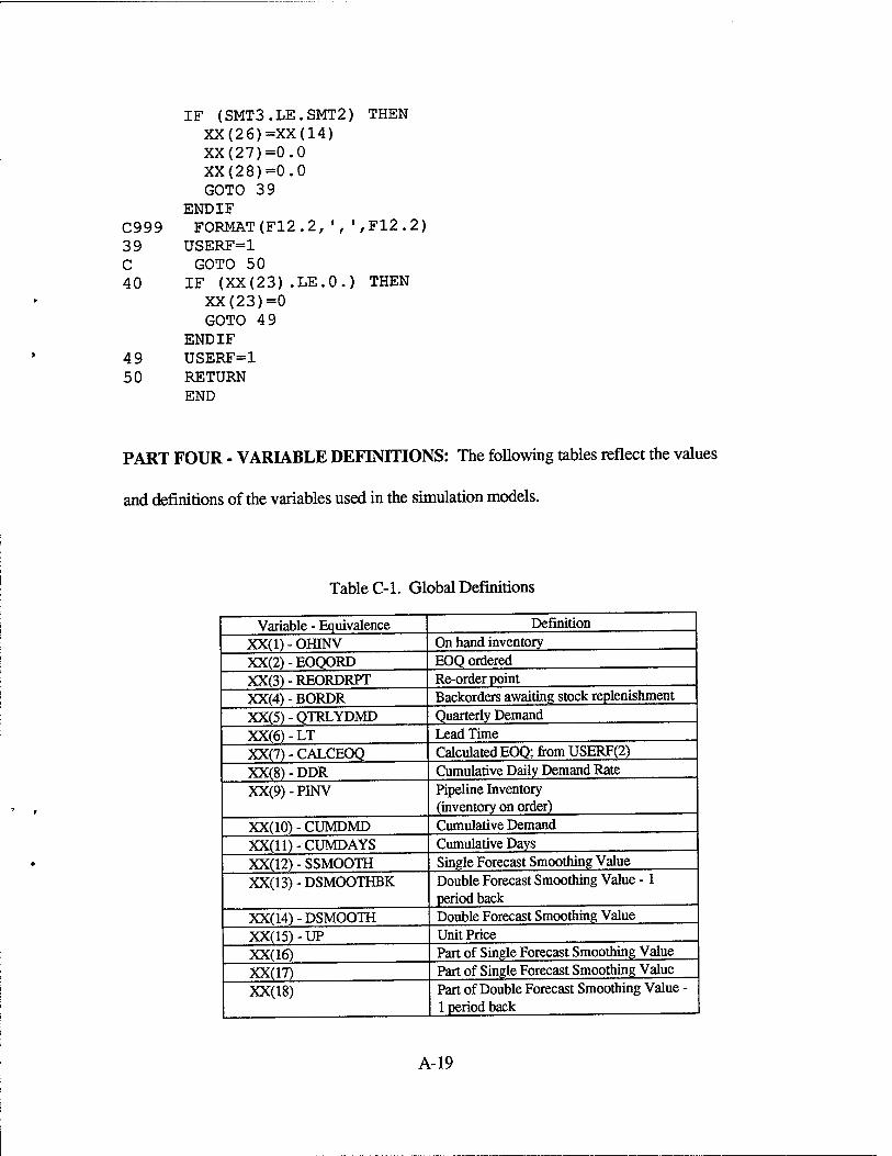
C999 39 C 40

49 50

IF (SMT3.LE.SMT2) THEN XX(26)=XX(14) XX(27)=0.0 XX(28)=0.0 GOTO 39

END IF FORMAT(F12.2,',',F12.2)

USERF=1 GOTO 50

IF (XX(23).LE.O.) THEN XX(23)=0 GOTO 4 9

END IF USERF=1 RETURN END

PART FOUR - VARIABLE DEFINITIONS: The following tables reflect the values

and definitions of the variables used in the simulation models.

Table C-l. Global Definitions

Variable - Equivalence Definition

XX(1) - OfflNV On hand inventory XX(2)-EOOORD EOQ ordered XX(3) - REORDRPT Re-order point XX(4) - BORDR Backorders awaiting stock replenishment

XX(5) - QTRLYDMD Quarterly Demand XX(6)-LT Lead Time

XX(7) - CALCEOO Calculated EOQ; from USERF(2)

XX(8) - DDR Cumulative Daily Demand Rate

XX(9)-PINV Pipeline Inventory (inventory on order)

XX(10)-CUMDMD Cumulative Demand XX(11)-CUMDAYS Cumulative Days XX(12) - SSMOOTH Single Forecast Smoothing Value

XX(13) - DSMOOTHBK Double Forecast Smoothing Value -1 period back

XX(14) - DSMOOTH Double Forecast Smoothing Value

XX(15) - UP Unit Price XX(16) Part of Single Forecast Smoothing Value

XX(17) Part of Single Forecast Smoothing Value

XX(18) Part of Double Forecast Smoothing Value - 1 period back

A-19

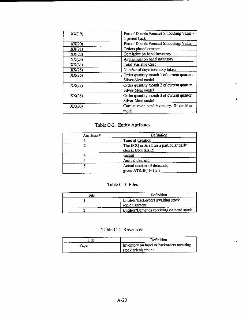
XX(19) Part of Double Forecast Smoothing Value - 1 period back

XX(20) Part of Double Forecast Smoothing Value XX(21) Orders placed counter XX(22) Cumlative on hand inventory XX(23) Avg annual on hand inventory XX(24) Total Variable Cost XX(25) Number of days inventory taken XX(26) Order quantity month 1 of current quarter.

Silver-Meal model XX(27) Order quantity month 2 of current quarter.

Silver-Meal model XX(28) Order quantity month 3 of current quarter.

Silver-Meal model XX(30) Cumlative on hand inventory. Silver-Meal

model

Table C-2. Entity Attributes

Attribute # Definition 1 Time of Creation 2 The EOQ ordered for a particular daily

check; from XX(2) 3 vacant 4 Annual demand 5 Actual number of demands,

given ATRIB(4)=1,2,3

Table C-3. Files

File Definition 1 Entities/Backorders awaiting stock

replenishment 2 Entities/Demands receiving on hand stock

Table C-4. Resources

File Definition Paper Inventory on hand or backorders awaiting

stock relenishment

A-20

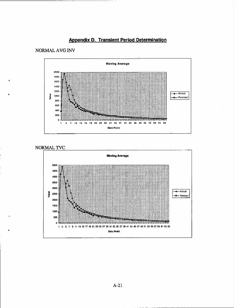
Appendix P. Transient Period Determination

NORMAL AVGINV

2000

1800

1600

1400

1200

1000

BOO

600

400

200

0

Moving Average

:H,Yn,fiTrrTrrTrTnTrr-rrrrrrrf-T,iTrtTrtTT,rrrr,n-rt

Actual

Forecast

7 10 13 16 19 22 25 28 31 34 37

Data Point

40 43 46 49 52 55 58 61 64

NORMAL TVC

Moving Average

-Actual

- Forecast

0 HWrWWWMWIWi^ffl^WlWWW-l^WI'Wt^WWWTWI'W't'fl

1 3 5 7 9 11 13 15 17 19 21 23 25 27 29 31 33 35 37 39 41 43 45 47 49 51 53 55 57 59 61 63 65

Data Pont

A-21

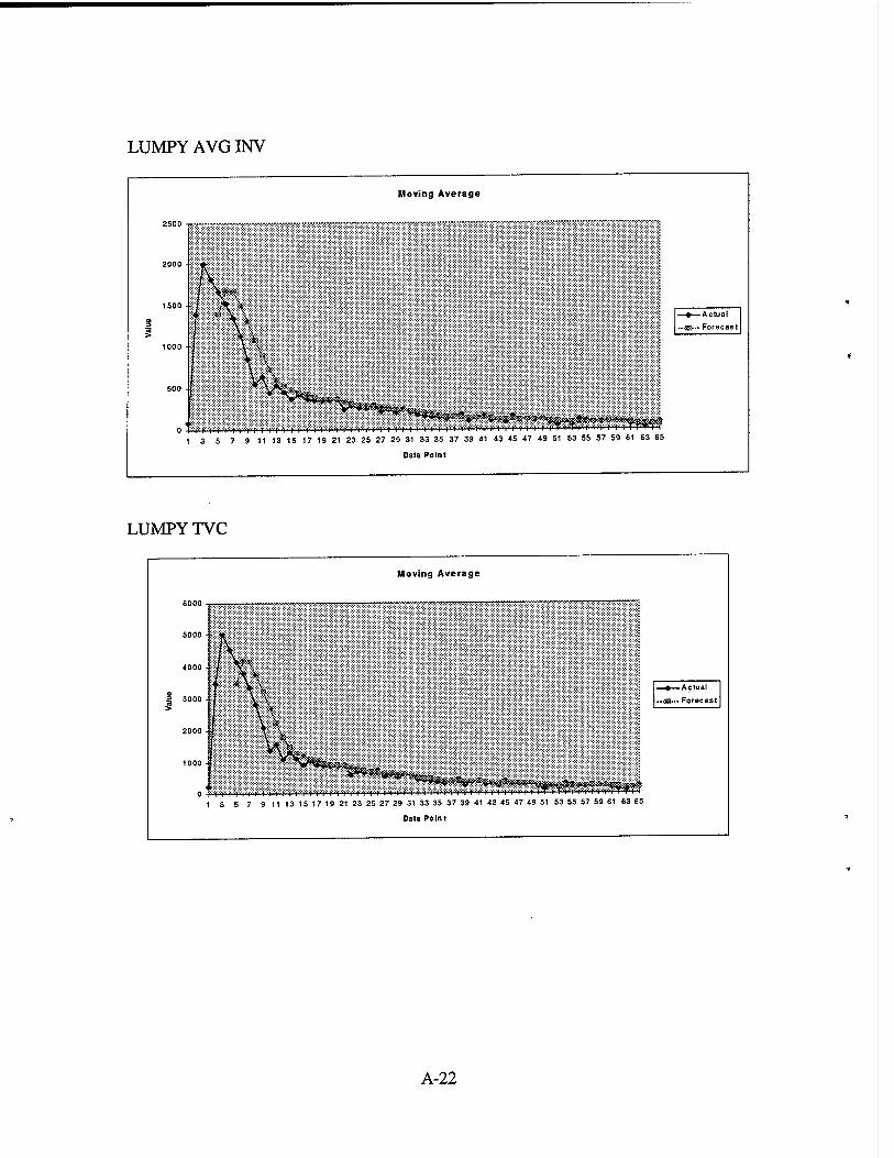
LUMPY AVGINV

Moving Average

»—Actual JJJ— Forecast

■fsw<wr<«ew(«r« 'I'M i > <■ i II i ><■!■>! ' i'l"l I i l l l )■ 3 5 7 9 11 13 15 17 19 21 23 25 27 29 31 33 35 37 39 41 43 45 47 49 51 53 55 57 59 61 63 65

LUMPY TVC

Moving Average

*— Actual

S— Forecast

7 9 11 13 15 17 19 21 23 25 27 29 31 33 35 37 39 41 43 45 47 49 51 53 55 57 59 61 63 65

Data Point

A-22

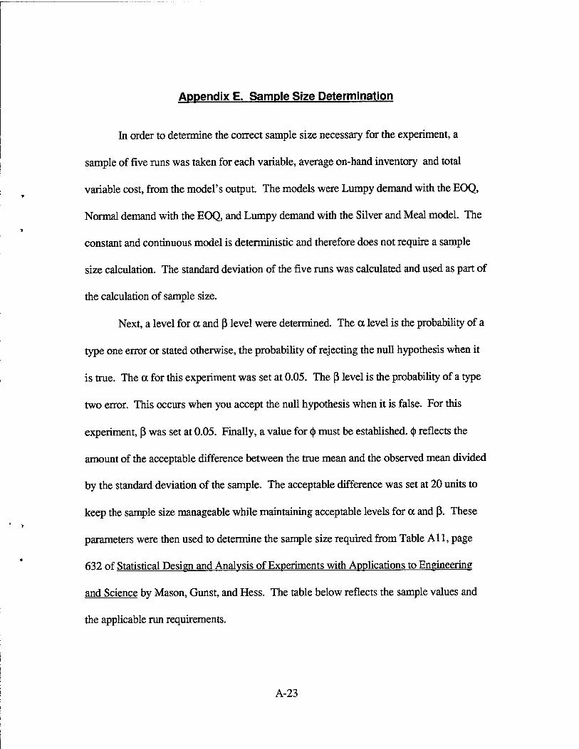
Appendix E. Sample Size Determination

In order to determine the correct sample size necessary for the experiment, a

sample of five runs was taken for each variable, average on-hand inventory and total

variable cost, from the model's output. The models were Lumpy demand with the EOQ,

Normal demand with the EOQ, and Lumpy demand with the Silver and Meal model. The

constant and continuous model is deterministic and therefore does not require a sample

size calculation. The standard deviation of the five runs was calculated and used as part of

the calculation of sample size.

Next, a level for a and ß level were determined. The a level is the probability of a

type one error or stated otherwise, the probability of rejecting the null hypothesis when it

is true. The a for this experiment was set at 0.05. The ß level is the probability of a type

two error. This occurs when you accept the null hypothesis when it is false. For this

experiment, ß was set at 0.05. Finally, a value for (J> must be established. (|> reflects the

amount of the acceptable difference between the true mean and the observed mean divided

by the standard deviation of the sample. The acceptable difference was set at 20 units to

keep the sample size manageable while maintaining acceptable levels for a and ß. These

parameters were then used to determine the sample size required from Table All, page

632 of Statistical Design and Analysis of Experiments with Applications to Engineering

and Science by Mason, Gunst, and Hess. The table below reflects the sample values and

the applicable run requirements.

A-23

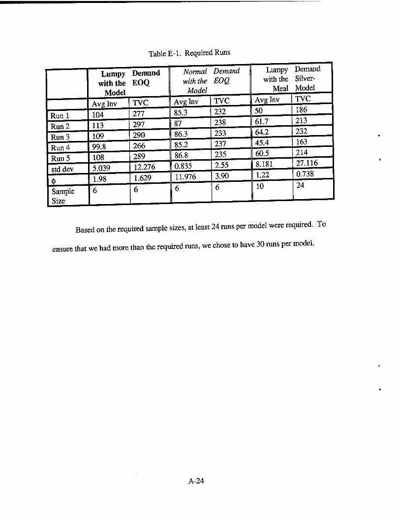
Runl Run 2 Run 3 Run 4 Run 5 std dev

A Sample Size

Table E-l. Required Runs

Lumpy Demand with the EOQ

Model Avglnv 104 113 109 99.8 108 5.039 1.98

TVC 277 297 290 266 289 12.276 1.629

Normal Demand with the EOQ

Model Avglnv 85.3

87 86.3 85.2

86.8 0.835 11.976

TVC 232 238 233 237 235

2.55

3.90

Lumpy Demand with the Silver-

Meal Model Avglnv 50 61.7 64.2 45.4 60.5 8.181 1.22 10

TVC 186 213 232 163 214 27.116 0.738 24

ensure

Based on the required sample sizes, at least 24 runs per model were required. To

that we had more than the required runs, we chose to have 30 runs per model.

A-24

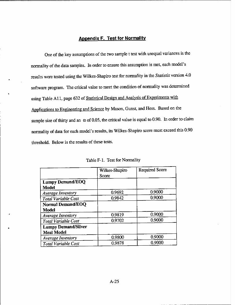
Appendix F. Test for Normality

One of the key assumptions of the two sample t test with unequal variances is the

normality of the data samples. In order to ensure this assumption is met, each model's

results were tested using the Wilkes-Shapiro test for normality in the Statistix version 4.0

software program. The critical value to meet the condition of normality was determined

using Table All, page 632 of Statistical Design and Analysis of Experiments with

Applications to Engineering and Science by Mason, Gunst, and Hess. Based on the

sample size of thirty and an a of 0.05, the critical value is equal to 0.90. In order to claim

normality of data for each model's results, its Wilkes-Shapiro score must exceed this 0.90

threshold. Below is the results of these tests.

Table F-l. Test for Normality

Wilkes-Shapiro Score

Required Score

Lumpy Demand/EOQ Model Average Inventory 0.9692 0.9000 Total Variable Cost 0.9842 0.9000 Normal Demand/EOQ Model Average Inventory 0.9819 0.9000 Total Variable Cost 0.9702 0.9000 Lumpy Demand/Silver Meal Model Average Inventory 0.9800 0.9000 Total Variable Cost 0.9878 0.9000

A-25

As one can see from the table, all the experimental results met the test of normality

and therefore, the t test is an acceptable test in this instance. As a side note, the Constant

and Continuous model does not meet the requirements of normality because it is a

deterministic model. Therefore, other nonparametric measures will be used to compare it

with other models.

A-26

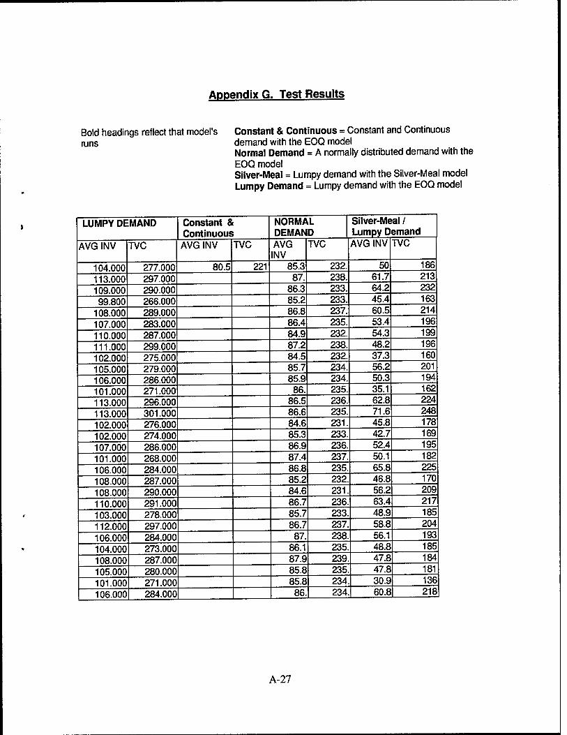
Appendix G. Test Results

Bold headings reflect that model's runs

Constant & Continuous = Constant and Continuous demand with the EOQ model Normal Demand = A normally distributed demand with the EOQ model Silver-Meal = Lumpy demand with the Silver-Meal model Lumpy Demand = Lumpy demand with the EOQ model

LUMPY DEMAND Constant & Continuous

NORMA DEMAN

L D

Silver-Meal / Lumpy Demand

AVG INV TVC AVG INV TVC AVG INV

TVC AVG INV TVC

104.000 277.000 80.5 221 85.3 232. 50 186

113.000 297.000 87. 238. 61.7 213

109.000 290.000 86.3 233. 64.2 232

99.800 266.000 85.2 233. 45.4 163

108.000 289.000 86.8 237. 60.5 214

107.000 283.000 86.4 235. 53.4 196

110.000 287.000 84.9 232. 54.3 199

111.000 299.000 87.2 238. 48.2 196

102.000 275.000 84.5 232. 37.3 160

105.000 279.000 85.7 234. 56.2 201

106.000 286.000 85.9 234. 50.3 194

101.000 271.000 86. 235. 35.1 162

113.000 296.000 86.5 236. 62.8 224

113.000 301.000 86.6 235. 71.6 248

102.000 276.000 84.6 231. 45.8 178

102.000 274.000 85.3 233. 42.7 169

107.000 286.000 86.9 236. 52.4 195

101.000 268.000 87.4 237. 50.1 182

106.000 284.000 86.8 235. 65.8 225

108.000 287.000 85.2 232. 46.8 170

108.000 290.000 84.6 231. 56.2 209

110.000 291.000 86.7 236. 63.4 217

103.000 278.000 85.7 233. 48.9 185

112.000 297.000 86.7 237. 58.8 204

106.000 284.000 87. 238. 56.1 193

104.000 273.000 86.1 235. 48.8 185

108.000 287.000 87.9 239. 47.8 184

105.000 280.000 85.8 235. 47.8 181

101.000 271.000 85.8 234. 30.9 136

106.000 284.000 86. 234. 60.8 218

A-27

Lumpy Demand Constant & Continuous

Normal Distribution

Silver-Meal / Lumpy

AVG INV TVC AVG INV TVC AVG INV

TVC AVG INV TVC

mean mean mean mean mean mean mean mean 106.360 283.533 80.5 221 86.093 234.667 52.470 193.967

stdev stdev stdev stdev stdev stdev stdev stdev

3.911 9.435 0 0 0.883 2.218 9.350 24.2806

A-28

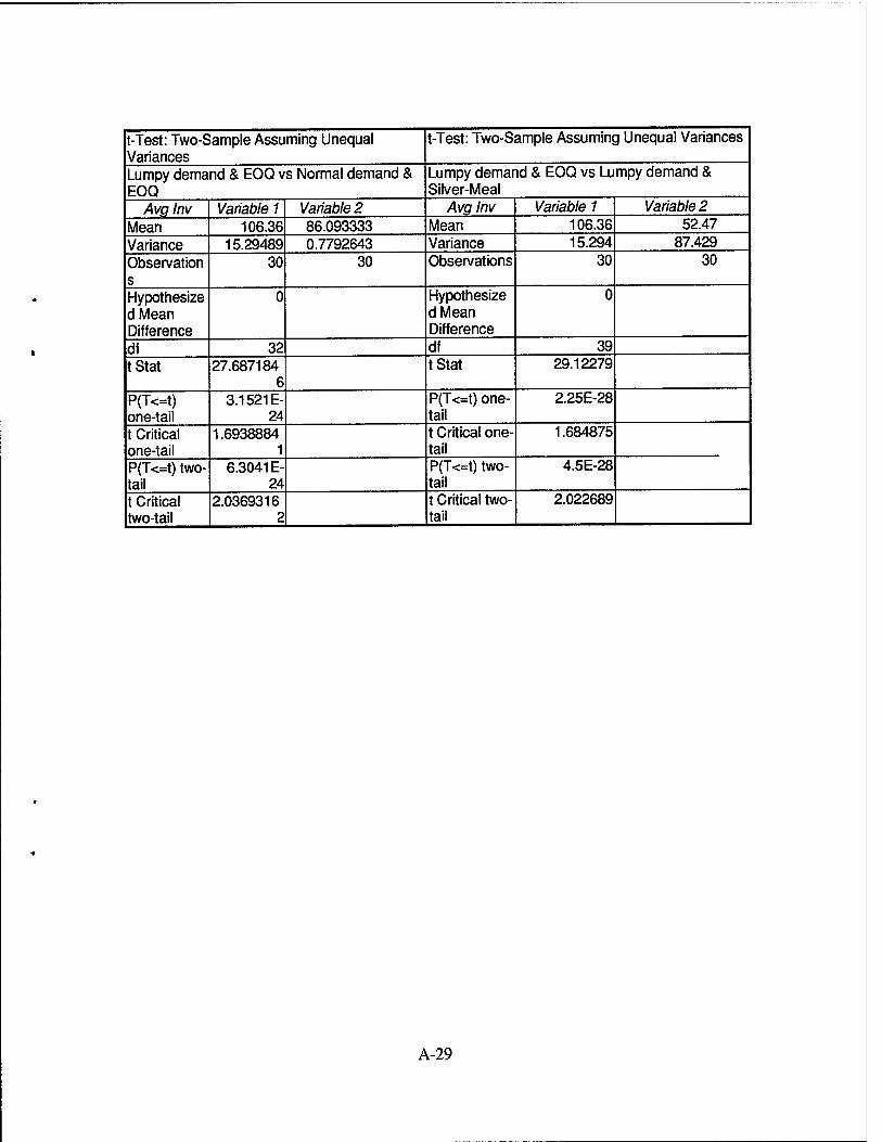
t-Test: Two-Sample Assuming Unequal Variances

t-Test: Two-Sample Assuming Unequal Variances

Lumpy demand & EOQ vs Normal demand & EOQ

Lumpy demand & EOQ vs Lumpy demand & Silver-Meal

Avg Inv Variable 1 Variable 2 Avg Inv Variable 1 Variable 2 Mean 106.36 86.093333 Mean 106.36 52.47 Variance 15.29489 0.7792643 Variance 15.294 87.429 Observation s

30 30 Observations 30 30

Hypothesize dMean Difference

0 Hypothesize dMean Difference

0

df 32 df 39 tStat 27.687184

6 tStat 29.12279

P(T<=t) one-tail

3.1521E- 24

P(T<=t) one- tail

2.25E-28

t Critical one-tail

1.6938884 1

t Critical one- tail

1.684875

P(T<=t) two- tail

6.3041 E- 24

P(T<=t) two- tail

4.5E-28

t Critical two-tail

2.0369316 2

t Critical two- tail

2.022689

A-29

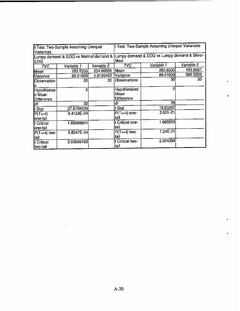
t-Test: Two-Sample Assuming Unequal Variances

t-Test: Two-Sample Assuming Unequal Variances

Lumpy demand & EOQ vs Normal demand & EOQ

Lumpy demand & EOQ vs Lumpy demand & Silver- Meal

TVC Variable 1 Variable 2 TVC Variable 1 Variable 2

Mean 283.5333 234.66666 Mean 283.5333 193.9667

Variance 89.01609 4.9195402 Variance 89.01609 589.5506

Observation s

30 30 Observations 30 30

Hypothesize dMean Difference

0 Hypothesized Mean Difference

0

df 32 df 38

tStat 27.6158339 tStat 18.83262

P(T<=t) one-tail

3.4124E-24 P(T<=t) one- tail

3.62E-21

t Critical one-tail

1.69388841 t Critical one- tail

1.685953

P(T<=t) two- tail

6.8247E-24 P(T<=t) two- tail

7.24E-21

t Critical two-tail

2.03693162 t Critical two- tail

2.024394

A-30

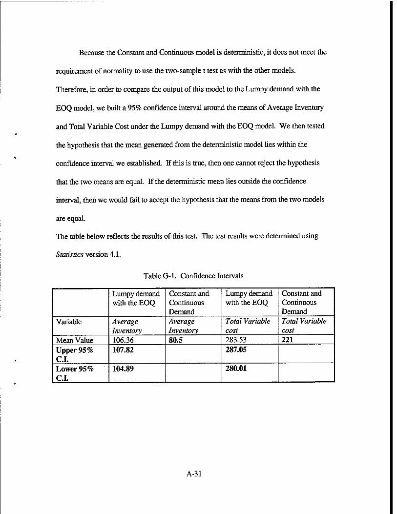
Because the Constant and Continuous model is deterministic, it does not meet the

requirement of normality to use the two-sample t test as with the other models.

Therefore, in order to compare the output of this model to the Lumpy demand with the

EOQ model, we built a 95% confidence interval around the means of Average Inventory

and Total Variable Cost under the Lumpy demand with the EOQ model. We then tested

the hypothesis that the mean generated from the deterministic model lies within the

confidence interval we established. If this is true, then one cannot reject the hypothesis

that the two means are equal. If the deterministic mean lies outside the confidence

interval, then we would fail to accept the hypothesis that the means from the two models

are equal.

The table below reflects the results of this test. The test results were determined using

Statistics version 4.1.

Table G-l. Confidence Intervals

Lumpy demand with the EOQ

Constant and Continuous Demand

Lumpy demand with the EOQ

Constant and Continuous Demand

Variable Average Inventory

Average Inventory

Total Variable cost

Total Variable cost

Mean Value 106.36 80.5 283.53 221 Upper 95% C.I.

107.82 287.05

Lower 95% C.I.

104.89 280.01

A-31

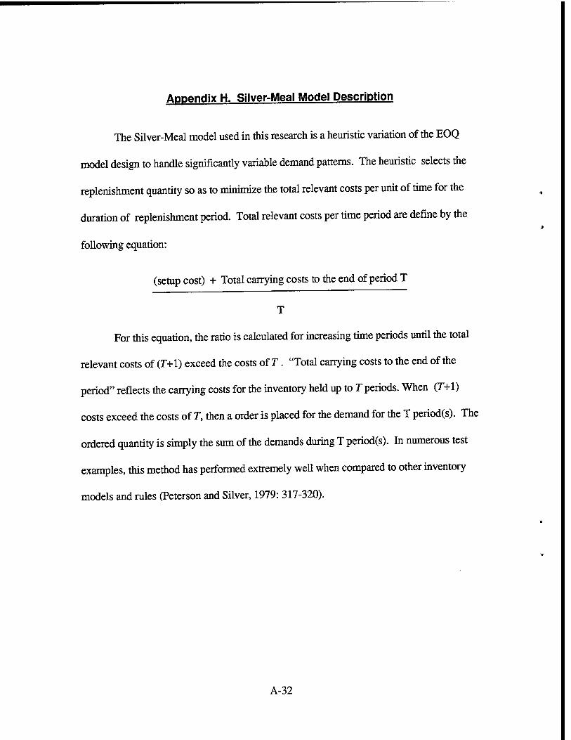
Appendix H. Silver-Meal Model Description

The Silver-Meal model used in this research is a heuristic variation of the EOQ

model design to handle significantly variable demand patterns. The heuristic selects the

replenishment quantity so as to minimize the total relevant costs per unit of time for the

duration of replenishment period. Total relevant costs per time period are define by the

following equation:

(setup cost) + Total carrying costs to the end of period T

T

For this equation, the ratio is calculated for increasing time periods until the total

relevant costs of (7>1) exceed the costs of T. "Total carrying costs to the end of the

period" reflects the carrying costs for the inventory held up to T periods. When (T+l)

costs exceed the costs of T, then a order is placed for the demand for the T period(s). The

ordered quantity is simply the sum of the demands during T period(s). In numerous test

examples, this method has performed extremely well when compared to other inventory

models and rules (Peterson and Silver, 1979: 317-320).

A-32

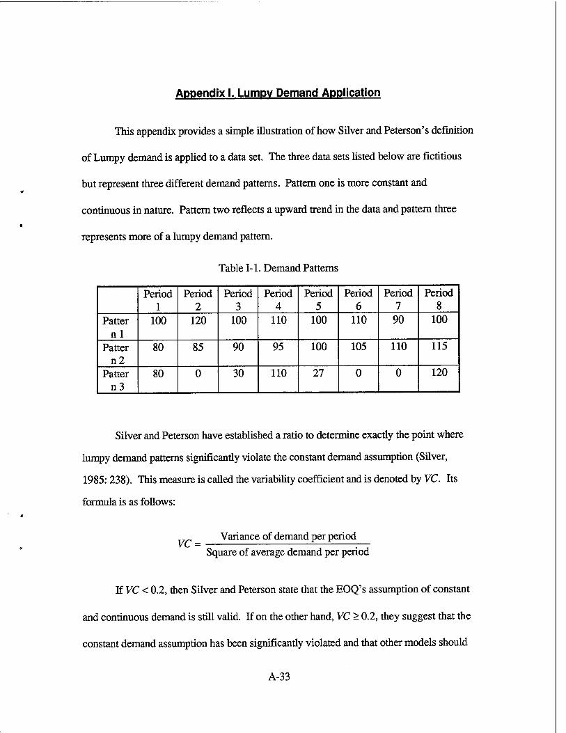
Appendix I. Lumpy Demand Application

This appendix provides a simple illustration of how Silver and Peterson's definition

of Lumpy demand is applied to a data set. The three data sets listed below are fictitious

but represent three different demand patterns. Pattern one is more constant and

continuous in nature. Pattern two reflects a upward trend in the data and pattern three

represents more of a lumpy demand pattern.

Table 1-1. Demand Patterns

Period 1

Period 2

Period 3

Period 4

Period 5

Period 6

Period 7

Period 8

Patter nl

100 120 100 110 100 110 90 100

Patter n2

80 85 90 95 100 105 110 115

Patter n3

80 0 30 110 27 0 0 120

Silver and Peterson have established a ratio to determine exactly the point where

lumpy demand patterns significantly violate the constant demand assumption (Silver,

1985: 238). This measure is called the variability coefficient and is denoted by VC. Its

formula is as follows:

VC = Variance of demand per period

Square of average demand per period

If VC < 0.2, then Silver and Peterson state that the EOQ's assumption of constant

and continuous demand is still valid. If on the other hand, VC > 0.2, they suggest that the

constant demand assumption has been significantly violated and that other models should

A-33

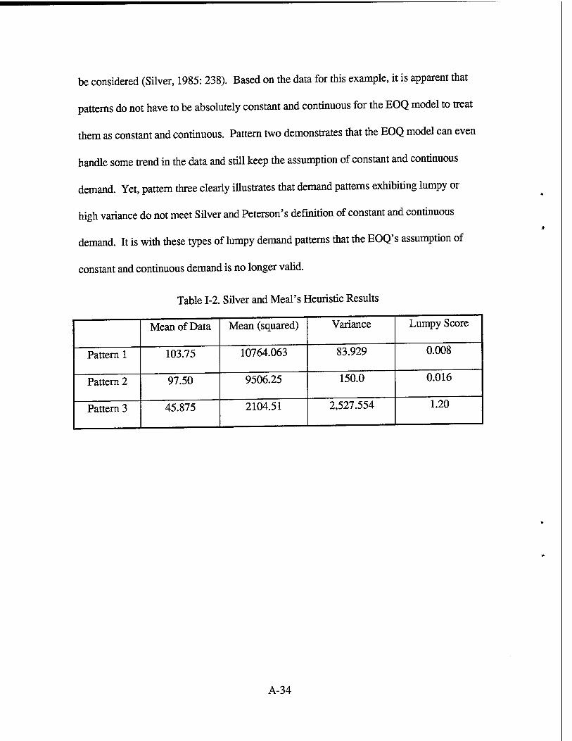
be considered (Silver, 1985: 238). Based on the data for this example, it is apparent that

patterns do not have to be absolutely constant and continuous for the EOQ model to treat

them as constant and continuous. Pattern two demonstrates that the EOQ model can even

handle some trend in the data and still keep the assumption of constant and continuous

demand. Yet, pattern three clearly illustrates that demand patterns exhibiting lumpy or

high variance do not meet Silver and Peterson's definition of constant and continuous

demand. It is with these types of lumpy demand patterns that the EOQ's assumption of

constant and continuous demand is no longer valid.

Table 1-2. Silver and Meal's Heuristic Results

Mean of Data Mean (squared) Variance Lumpy Score

Pattern 1 103.75 10764.063 83.929 0.008

Pattern 2 97.50 9506.25 150.0 0.016

Pattern 3 45.875 2104.51 2,527.554 1.20

A-34

Appendix J. Graph of Lead Time Pattern

Lead Time (days)

■H—t—i—I—I—I—h

3 5 7 9 11 13 15 17 19 21 blocks 30..720

^Frequency

The lead time chart above represents a histogram (number of demands or hits of a

particular demand value) of the average lead time for all the items in the sample data.

Each block on the x-axis has a width of 30 observations. For the first block 98 items have

a lead time of less than thirty days. All of the data points are represented in this graph.

A-35

References

APICS Dictionary. American Production and Inventory Control Society Dictionary (Seventh Edition). Falls Church VA: The Society. 1992.

Balwally, Nandakumar M. Operations Research Analysis and Projects Division, Defense Electronics Supply Center (DESC/EIR), Dayton OH. Telephone Interview. 12 December 1994.

Bilikan, Robert. Operations Research Analysis and Projects Division, Defense Electronics Supply Center (DESC/EIR), Dayton OH. Telephone Interview. 12 December 1994.

Blazer, Douglas J. "Variability of Demand: Why the Part is Never on the Shelf", Air Force Journal of Logistics. 11-22 (Spring,1985).

Choi, Richard H., Eric M. Malstrom, and Russell D. Tsai. "Evaluating Lot-sizing Methods in Multilevel Inventory Systems by Simulation," Production and Inventory Management Journal. 4-10 (Fourth Quarter, 1988).

Clark, Andrew J. "A Multiechelon, Dynamic Inventory Model," Naval Logistics Quarterly. 429-445 (Second Quarter, 1993).

Cooper, Donald E. and William Emory. Business Research Methods (Fifth Edition). Chicago: Irwin Incorporated, 1995.

Coyle, John J., Edward J. Bardi and C. John Langley, Jr. The Management of Business Logistics (Fifth Edition). New York: The West Publishing Company, 1988.

Defense Logistics Agency, Document DL107-2/11/91,2-1.

Delugio, Stephen A. and Carl D. Bhane. "Integrating Forecasts and Inventory Management of Low Volume Demands", 34th International Conference Proceedings. American Production and Inventory Control Society. Seattle: PALM Press, 1991.

Harding, Michael. "Why Manage Inventory?" American Production and Inventory Control Society, 33rd International Conference Procedings, Vol: 42-247, (Oct 1990).

REF-1

Hood, William C. A Handbook of Supply Inventory Models. MS Thesis, AFIT/GLM/LSMA/87S-35. School of Systems and Logistics, Air Force Institute of Technoloy (AU), Wright-Patterson AFB OH, September 1987 (AD-A187269)

Knowles, Thomas W. Management Science, Building and Using Models Hinois: Irwin Incorporated, 1989.

Law, Averill M. and W. David Kelton. Simulation Modeling and Analysis (Second Edition). New York: McGraw-Hill Incorporated, 1991.

Long, William S. and Douglas H. Engberson, The Effect of Violations of the Constant Demand Assumption on the Defense Logistic Agency Requirements Model. MS Thesis, AFIT/GLM/LAL/94S-15. School of Systems and Logistics, Air Force Institute of Technoloy (AU), Wright-Patterson AFB OH, September 1994 (AD-A285272).

McClave, James T. and P. George Benson. Statistics for Business and Economics (Sixth Edition). New York: Macmillen College Publishing Company, 1994.

Miller, George J. CPIM, "Inventory Reduction," American Production and Inventory Control Society, 33rd International Conference Procedings, Vol:242-247, (Oct 1990).

Madsen, Richard W., and Melvin L. Moeschberger. Statistical Concepts With Applications to Business and Economics. Prentice-Hall, Incorporated, New Jersey, 1980.

Makridakis, Spyros and Wheelwright, Steven C. Forecasting Methods for Management (Fifth Edition). New York: John Wiley & Sons, 1989.

Montgomery, Douglas C. Design and Analysis of Experiments (Third Edition). New York: John Wiley & Sons, 1991.

Peterson, Rein and Edward A. Silver. Decision Systems For Inventory Management and Production Planning. New York: John Wiley & Sons, 1979.

Prichard, James W. and Robert H. Eagle, Modem Inventory Management. New York: John Wiley & Sons, 1965.

Pritsker, Alan B. Introduction to Simulation and SLAM U (Third Edition). New York: Systems Publishing Corporation, 1986.

REF-2

Robinson, Nathaniel. The Defense Logistics Agency. Providing Logistics Support Throughout the Department of Defense. Research Report No. AU-ARI-92-4. Maxwell Air Force Base AL. Air University Press, October 1993.

Shields, Mathew D. "Economic Order Quantity and the Air Force." PhD Course Essay. The Ohio State University, Columbus OH, 1990.

Siegel, Joan. Statistix, Version 4.0. Tallahassee: Analytical Software, 1992.

Silver, Edward A. and Rein Peterson. Decision Systems for Inventory Management and Production Planning (2nd Edition). New York: John Wiley and Sons, 1985. 237-238.

Tersine, Richard J. Principles of Inventory and Materials Management (4th Edition). New Jersey: PTR Prentice Hall, 1994.

REF-3

Berry Vita

Captain Harry A. Berry is from Salt Lake City, Utah. He graduated from the

University of Utah in 1984 with a Bachelor of Science degree in Finance and again in 1986

with a Master's degree in Business Administration. After receiving his commission into

the United States Air Force in 1987 through the Officers Training School, Captain Berry

was assigned to the 27th Supply Squadron at Cannon AFB, New Mexico.

During his tour at Cannon AFB, Captain Berry served as the Chief, AGS Parts

Store in support of the F-l 1 ID and subsequently, Chief, Materiel Management Branch. In

1989, he was assigned to the 15th Supply Squadron at Hickam AFB, Hawaii. During his

tour in Hawaii, Captain Berry filled a variety of positions within the squadron. These

positions included Chief, Operations Support Branch, Chief, Materiel Management

Branch, and Chief, Management and Systems Right.

In 1994, Captain Berry entered the Air Force Institute of Technology at Wright-

Patterson AFB, Ohio, and graduated in 1995 with a Masters degree in Logistics

Management. He was subsequently assigned to the Logistics Management Agency,

Maxwell AFB, Alabama.

Captain Berry and his wife Sandy were married on August 27,1983 and have a

daughter Sarah, age 8, a son Ryan, age 5, and another son Conner, age 1.

Permanent Address: 41 Meehan Drive Dayton, OH. 45431

V-l

Tatae Vita

Captain Edward E. Tatge is from Piano, Texas. He graduated from the East Texas

State University in 1989 with a Bachelor of Science degree in Computer Science and

Math. After receiving his commission into the United States Air Force through the

Reserve Officers Training Corps, Captain Tatge was assigned to the 4 Supply Squadron, 4

Wing at Seymour Johnson AFB, North Carolina.

During his tour at Seymour Johnson AFB, Captain Tatge filled a variety of supply

positions in support of the F-15E and KC-10 aircraft. These positions included OIC of

Supply Readiness Control Center, and OIC War Readiness Section. During this

assignment, Captain Tatge deployed with the 4 Wing in support of Operation Desert

Shield and Desert Storm.

In 1992, he was assigned to Shaw AFB, South Carolina, where he served nearly

two years on the US Central Command Air Forces (USCENTAF) Staff as the Supply,

Management and Systems Branch Chief. Capt Tatge was selected into the Air Force

Institute of Technology at Wright-Patterson AFB, Ohio in May 1994 and graduated with a

Masters degree in Logistics Management in September 1995. He was subsequently

assigned to the Logistics Management Agency, Maxwell AFB, Gunter Annex, Alabama.

Permanent Address: 3823 Butterfield Dr. Beavercreek, OH. 45431

V-2

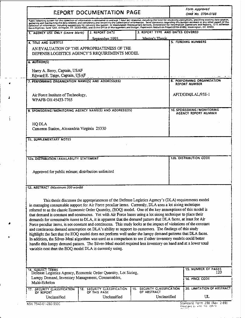
REPORT DOCUMENTATION PAGE Form Approved

OMB No. 0704-0188

Public reporting burden for this collection of information is estimated to average i hour per respome. including the lime tor reviewing instructions, searching existing data sources, gathering and maintaining the data needed, and completing and reviewing the collection o( information. Send comments regarding this burden ««mate or any other aspect of this collection of information including suggestions for reducing this Burden, to Washington Headquarters Services. Directorate tor Information Operations and Reports. 1215 Jefferson Davis Highway. Suite 1204. Arlington. VA 22202-4302. and to the OHice o' Management and Budget. Paperwork Reduction Proiect (0704-0188). Washington. DC 20503.

3. REPORT TYPE AND DATES COVERED 1. AGENCY USE ONLY (Leave blank) 2. REPORT DATE

,Sppmmhr,r1991 Mastpr'i Thpgic;

4. TITLE AND SUBTITLE

AN EVALUATION OF THE APPROPRIATENESS OF THE DEFENSE LOGISTICS AGENCY'S REQUIREMENTS MODEL

fi. AUTHOR(S)

Harry A. Berry, Captain, USAF Edward E.Tatge, Captain, USAF .

7. PERFORMING ORGANIZATION NAME(S) AND ADDRESS(ES)

Air Force Institute of Technology, WPAFB OH 45433-7765

9. SPONSORING /MONITORING AGENCY NAME(S) AND ADDRESS(ES)

HQDLA Cameron Station, Alexandria Virginia 25330

5. FUNDING NUMBERS

PERFORMING ORGANIZATION REPORT NUMBER

AHT/GIM/LAL/95S-1

10. SPONSORING/MONITORING AGENCY REPORT NUMBER

It. SUPPLEMENTARY NOTES

n2a. DISTRIBUTION / AVAILABILITY STATEMENT

Approved for public release; distribution unlimited

12b. DISTRIBUTION CODE

13. ABSTRACT (Maximum 200 words)

This thesis discusses the appropriateness of the Defense Logistics Agency's (DLA) requirements model in managing consumable support for Air Force peculiar items. Currently, DLA uses a lot sizing technique referred to as the classic Economic Order Quantity, (EOQ) model. One of the key assumptions of this model is that demand is constant and continuous. Yet with Air Force bases using a lot sizing technique to place their demands for consumable items to DLA, it is apparent that the demand pattern that DLA faces, at least for Air Force peculiar items, is not constant and continuous. This study looks at the impact of violations of the constant and continuous demand assumption on DLA's ability to support its customers. The findings of this study highlight the fact that the EOQ model does not perform well under the lumpy demand patterns that DLA faces. In addition, the Silver-Meal algorithm was used as a comparison to see if other inventory models could better handle this lumpy demand pattern. The Silver-Meal model required less inventory on hand and at a lower total variable cost than the EOQ model DLA is currently using.

"14. SUBJECT TERMS Defense Logistics Agency, Economic Order Quantity, Lot Sizing, Lumpy Demand, Inventory Management, Consumables, Multi-Echelon

17. SECURITY CLASSIFICATION OF REPORT

Unclassified

18. SECURITY CLASSIFICATION OF THIS PAGE

Unclassified

IS. SECURITY CLASSIFICATION OF ABSTRACT

Unclassified

15. NUMBER OF PAGES 120

16. PRICE CODE

20. LIMITATION OF ABSTRACT I I

UL

NSN 7540-0'i-2SO-5500 Stanoarc form 298 (Rev 2-89)