air force institute of technology - dtic
TRANSCRIPT

RAMAN SCATTERING STUDY OF SUPERCRITICAL BI-COMPONENT MIXTURES INJECTED INTO A SUBCRITICAL ENVIRONMENT
THESIS
Young Man An, Captain, ROKA
AFIT/GA/ENY/07-S01
DEPARTMENT OF THE AIR FORCE AIR UNIVERSITY
AIR FORCE INSTITUTE OF TECHNOLOGY
Wright-Patterson Air Force Base, Ohio
APPROVED FOR PUBLIC RELEASE; DISTRIBUTION UNLIMITED

The views expressed in this thesis are those of the author and do not reflect the official
policy or position of the United States Air Force, Department of Defense, or the U.S.
Government.
AFIT/GA/ENY/07-S01
RAMAN SCATTERING STUDY OF SUPERCRITICAL BI-COMPONENT MIXTURES INJECTED INTO A SUBCRITICAL ENVIRONMENT
THESIS
Presented to the Faculty
Department of Aeronautics and Astronautics
Graduate School of Engineering and Management
Air Force Institute of Technology
Air University
Air Education and Training Command
In Partial Fulfillment of the Requirements for the
Degree of Master of Science in Astronautical Engineering
Young Man An, BS
Captain, ROKA
September 2007
APPROVED FOR PUBLIC RELEASE; DISTRIBUTION UNLIMITED

AFIT/GA/ENY/07-S01
RAMAN SCATTERING STUDY OF SUPERCRITICAL BI-COMPONENT MIXTURES INJECTED INTO A SUBCRITICAL ENVIRONMENT
Young Man An, BS
Captain, ROKA
Approved: /signed/ 5 September 2007 ____________________________________ ________ Paul I. King Date /signed/ 5 September 2007 ____________________________________ ________ Richard D. Branam Date /signed/ 5 September 2007 ____________________________________ ________ Mark F. Reeder Date

AFIT/GA/ENY/07-S01
Abstract
This research studies the species distribution profiles of methane/ethylene bi-
components at downstream locations filled with subcritical nitrogen in a closed chamber.
Unique thermodynamic and transport properties of supercritical fluids along with phase
transition phenomena during fuel injection process can significantly change combustion
characteristics inside a scramjet combustor. Plume properties of supercritical jets are of
great interests to the studies of fuel/air mixing and subsequent combustion. The primary
goal of this research is to help to clarify whether there is any preferential condensation
within the condensed jets. The Raman Scattering technique is used to quantify spatial
distribution of injected methane and ethylene. Each species distribution profile is
developed in terms of mole fraction. Results demonstrated there is ethylene preferential
condensation within the supercritical bi-component mixture of the jet. It also showed the
condensation phenomenon is less desirable for combustion.
iv

v
AFIT/GA/ENY/07-S01
To My Great Country, Korea, and My Lovely Wife and Sons

Acknowledgments
The scope what was accomplished in this work far exceeded my own vision, and
would not have been possible without patient instruction of many along the way.
I would like to express my sincere appreciation to my faculty advisor, Dr. Paul
King for his guidance and encouragement throughout this effort and advising at key
points. My appreciation also to my faculty members, Major Richard Branam, Dr. Mark
Reeder for their critical advises.
I also would like to thank my sponsor, Dr. Mike Ryan, from the Air Force
Propulsion Directorate for the support and knowledge that he provided me. Dr. Mike
Ryan provided the patient teaching and the proper guidance form all the basics and presented
genuine interest in the experiment to make this thesis an enjoyable experience.
Finally, I would like to give a great thanks to my lovely wife. Without her
continuous support and dedication, I would not have achieved what I have in my life.
Thank you for supporting and being with me throughout this long journey, once again.
In addition, there were many who provided assistance along the way. I would like
thank the laboratory technicians, John Hixenbaugh for getting me out of trouble and his
friendship.
Young Man, An
iv

Table of Contents
Page Abstract ...................................................................................................................... iv Acknowledgements .................................................................................................... iv Table of Contents .........................................................................................................v List of Figures ........................................................................................................... viii List of Tables ........................................................................................................... xiv Nomenclature...............................................................................................................xv I. Introduction .............................................................................................................1 Background.............................................................................................................1 Problem Statement ..................................................................................................4 Research Objectives................................................................................................5 Research Focus .......................................................................................................5 Methodology...........................................................................................................6 II. Literature Review....................................................................................................7 Chapter Overview ..................................................................................................7 Relevant Research..................................................................................................7 Supercritical Region ..........................................................................................8 Phase Transition ................................................................................................9 Characteristics of the Near-Field Jet ..............................................................11 Mixing Characteristics at the Downstream of the ethylene Jet .......................12 Jet Flow................................................................................................................13 Raman Spectroscopy............................................................................................14 Nature of Raman Scattering.............................................................................14 Electromagnetic Wave .....................................................................................15 Classical Theory Overview ..............................................................................16 Shadowgraph Imaging System ............................................................................26 III. Methodology........................................................................................................28 Chapter Overview................................................................................................28 Apparatus ............................................................................................................29 Instrumentation ....................................................................................................33 Raman Scattering System.................................................................................33 Shadowgraph Imaging System .........................................................................35
v

Page Calibration ...........................................................................................................36 Experimental Procedure.......................................................................................41 Overview ..........................................................................................................41 Shadowgraph ...................................................................................................42 Raman Scattering ............................................................................................42 Testing Strategy ...................................................................................................43 Data Processing....................................................................................................45 Shadowgraph Image ........................................................................................45 Raman Scattering Data ...................................................................................47 IV. Results and Discussion ..........................................................................................53 Chapter Overview ................................................................................................53 Shadowgraph Results...........................................................................................54 Supercritical Ethylene Fuel Injection ..............................................................54 Supercritical Methane and Ethylene Mixture (XCH4 = 0.1) Fuel Injection......68 Raman Scattering Results ....................................................................................77 Supercritical Ethylene Fuel Injection ..............................................................78 Supercritical Methane and Ethylene Mixture (XCH4 = 0.2) Fuel Injection......84 Supercritical Methane and Ethylene Mixture (XCH4 = 0.1) Fuel Injection......90 Ethylene Mole Fractions for Different Nozzles ...........................................91 Normalized Ethylene Mole Fractions ..........................................................96 Ethylene Mole Fractions for Different Injection Temperatures ..................99 Methane Mole Fractions for Different Nozzles .........................................103 Nitrogen Mole Fractions for Different Nozzles .........................................106 Mole Fraction Ratios of Ethylene to Methane for Different Nozzles.........108 Jet Divergence Angle and Potential Core Length..............................................112 V. Conclusions and Recommendations ...................................................................114 Conclusions........................................................................................................114 Experiment Overview..................................................................................114 Conclusions.................................................................................................114 Recommendations for Future Research .............................................................117 Appendix A. Injection Nozzle Design .....................................................................118 Appendix B. Least Square Method ...........................................................................121 Appendix C. Supercritical Fuel Injection System and Operating Procedure.............122 Appendix D. Jet Divergence Angle Equation............................................................129
vi

Appendix E. Ethylene Vibrational Mode...................................................................130 References..................................................................................................................132 Vita.............................................................................................................................134
vii

List of Figures
Figure Page 1. Maximum Estimated Excess Heat Loads for Various Aircraft ..............................2
2. Cooling Capacity of Various Fuels.........................................................................3 3. Critical temperature and pressure diagram of different methane/ethylene mixture
fuel from SUPERTRAPP Program..........................................................................9 4. Entropy-pressure phase diagram for the methane/ethylene mixture, XCH4 = 0.1,
from the SUPERTRAPP program. ........................................................................10 5. Condensation phenomena for different temperature ratios at the same pressure
ratios (a). Jet expansion angles for different pressure ratios at the same temperatures (b). ....................................................................................................10
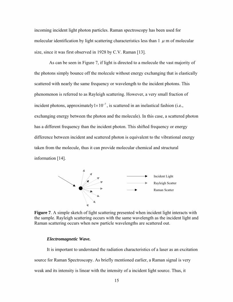
6. Nitrogen injection shadowgraph image for jet flow structure ..............................13 7. A simple sketch of light scattering presented when incident light interacts with
the sample. Rayleigh scattering occurs with the same wavelength as the incident light and the Raman scattering occurs when new particle wavelengths are scattered out. ..........................................................................................................15
8. Electromagnetic radiation .....................................................................................16 9. Polarization (P) induced in a molecule’s electron cloud by an incident optical
electric field E. ......................................................................................................17 10. (a) Simplified energy diagrams, (b) Schematics of a Raman spectrum..............19 11. Illustration of the behavior of a reflection phase grating....................................23 12. Schematic of spectrometer system......................................................................24 13. Schematic of a CCD Detector for 512×512 pixel array......................................25 14. Example of Raman shift of bi-species medium. ..................................................25 15. Schematic of the Shadowgraph technique for 2-D transparent flow.. .................26 16. Sketches of Supercritical fuel injection apparatus.. .............................................30
viii

Figure Page 17. Sketch of the nozzles used for this study, d = 0.5mm ........................................31
18. Schematic of Raman spectroscopy instrumentation ...........................................33 20. Direct shadowgraph imaging instrumentation. ...................................................35 21. Neon calibration image, number counts on the vertical-axis versus wavenumber
on the horizontal-axis.............................................................................................37 22. Calibration curve fit of Raman scattering signal…………………..……………40 23. (a) The raw shadowgraph image data, (b) Averaged, (c) Filtered ......................46 24. (a) Raman Image, (b) Intensity profile along the y-axis .....................................48 25. 3-D signal intensity profile by Image J surface plot ...........................................49 26. Different background intensity profile. (a) Ethylene calibration data, (b) XCH4 =
0.1 mixture data, (c) Background intensity profile. ...............................................51 27. Shadowgraph image injection conditions, ethylene fuel. ...................................55 28. Shadowgraph image, ethylene, nozzle #8, d = 1mm, Tr = 1.01, Pr = 1.01 ..........57
29. Shadowgraph image, ethylene, nozzle #8, d = 1mm, Tr = 1.04, Pr = 1.01. ..........57 30. Shadowgraph image, ethylene, nozzle #8, d = 1mm, Tr = 1.08, Pr = 1.02.. .........58 31. Shadowgraph image, ethylene, Nozzle #1, d = 0.5mm, Tr = 1.00, Pr = 1.03.. .....60 32. Shadowgraph image, ethylene, nozzle #1, d = 0.5mm, Tr = 1.01, Pr = 1.03. .......60 33. Shadowgraph image, ethylene, nozzle #1, d = 0.5mm, Tr = 1.02, Pr = 1.03 ........61
34. Shadowgraph image, ethylene, nozzle #1, d = 0.5mm, Tr = 1.03, Pr = 1.03. .......61 35. Shadowgraph image, ethylene, nozzle #6, d = 0.5mm, Tr = 1.00 Pr = 1.04.. .......62 36. Shadowgraph image, ethylene, nozzle #6, d = 0.5mm, Tr = 1.01 Pr = 1.03... ......62 37. Shadowgraph image, ethylene, nozzle #6, d = 0.5mm, Tr = 1.02 Pr = 1.03.. .......63
ix

Figure Page 38. Shadowgraph image, ethylene, nozzle #6, d = 0.5mm, Tr = 1.03 Pr = 1.03.... .....63 39. Shadowgraph image, ethylene, nozzle #7, d = 0.5mm, Tr = 1.00 Pr = 1.02... ......64 40. Shadowgraph image, ethylene, nozzle #7, d = 0.5mm, Tr = 1.01 Pr = 1.03 ........64
41. Shadowgraph image, ethylene, nozzle #7, d = 0.5mm, Tr = 1.02, Pr = 1.03 .......65 42. Shadowgraph image, ethylene, nozzle #7, d = 0.5mm, Tr = 1.03, Pr = 1.03. ......65 43. Shadowgraph image, ethylene, nozzle #9, d = 0.5mm, Tr = 1.00, Pr = 1.03 .......66 44. Shadowgraph image, ethylene, nozzle #9, d = 0.5mm, Tr = 1.01 Pr = 1.03 ........66 45. Shadowgraph image, ethylene, nozzle #9, d = 0.5mm, Tr = 1.02 Pr = 1.03 ........67 46. Shadowgraph image, ethylene, nozzle #9, d = 0.5mm, Tr = 1.04 Pr = 1.02 ........67 47. Shadowgraph image injection conditions, XCH4 = 0.1 mixture fuel. ..................68 48. Shadowgraph image, XCH4 = 0.1, nozzle #1, d = 0.5mm, Tr = 1.00, Pr = 1.04. ..69 49. Shadowgraph image, XCH4 = 0.1, nozzle #1, d = 0.5mm, Tr = 1.01, Pr = 1.04 ...69
50. Shadowgraph image, XCH4 = 0.1, nozzle #1, d = 0.5mm, Tr = 1.02, Pr = 1.04. ...70 51. Shadowgraph image, XCH4 = 0.1, nozzle #1, d = 0.5mm, Tr = 1.04, Pr = 1.04... .70 52. Shadowgraph image, XCH4 = 0.1, nozzle #6, d = 0.5mm, Tr = 1.00, Pr = 1.04... .71 53. Shadowgraph image, XCH4 = 0.1, nozzle #6, d = 0.5mm, Tr = 1.01, Pr = 1.04. ...71 54. Shadowgraph image, XCH4 = 0.1, nzzle #6, d = 0.5mm, Tr = 1.02, Pr = 1.03 ......72
55. Shadowgraph image, XCH4 = 0.1, nozzle #6, d = 0.5mm, Tr = 1.04, Pr = 1.03. ...72 56. Shadowgraph image, XCH4 = 0.1, nozzle #7, d = 0.5mm, Tr = 1.00, Pr = 1.01... .73 57. Shadowgraph image, XCH4 = 0.1, nozzle #7, d = 0.5mm, Tr = 1.01, Pr = 1.04... .73 58. Shadowgraph image, XCH4 = 0.1, nozzle #7, d = 0.5mm, Tr = 1.03, Pr = 1.04... .74 59. Shadowgraph image, XCH4 = 0.1, nozzle #7, d = 0.5mm, Tr = 1.04, Pr = 1.03... .74
x
Figure Page 60. Shadowgraph image, XCH4 = 0.1, nozzle #9, d = 0.5mm, Tr = 1.00, Pr = 1.04... .75 61. Shadowgraph image, XCH4 = 0.1, nozzle #9, d = 0.5mm, Tr = 1.01, Pr = 1.01 ...75
62. Shadowgraph image, XCH4 = 0.1, nozzle #9, d = 0.5mm, Tr = 1.03, Pr = 1.04 ..76 63. Shadowgraph image, XCH4 = 0.1, nozzle #7, d = 0.5mm, Tr = 1.04, Pr = 1.03...76 64. Ethylene to methane mole fraction ratios of XCH4 = 0.1, 0.2 mixture fuel without
injection..................................................................................................................78 65. Raman scattering injection conditions, ethylene fuel .........................................79 66. Ethylene mole fraction, ethylene, nozzle #1.......................................................82 67. Ethylene mole fraction, ethylene, nozzle #1, without accumulated number
density. ...................................................................................................................82 68. Normalized ethylene mole fraction, ethylene, nozzle #1....................................83
69. Nitrogen mole fraction, ethylene, nozzle #1... .....................................................83 70. Raman scattering injection conditions, XCH4 = 0.2 mixture fuel, nozzle #1…....84 71. Ethylene mole fraction, XCH4 = 0.2 mixture, nozzle #1... ....................................85 72. Ethylene mole fraction, XCH4 = 0.2 mixture, nozzle #1, without accumulated
number density.......................................................................................................86 73. Normalized ethylene mole fraction, XCH4 = 0.2 mixture, nozzle #1... .................86 74. Methane mole fraction, XCH4 = 0.2 mixture, nozzle #1.. .....................................87 75. Nitrogen mole fraction, XCH4 = 0.2 mixture, nozzle #1. ......................................87 76. Ethylene to methane mole fraction ratio of XCH4 = 0.2 mixture fuel, nozzle #1. 88 77. Raman scattering injection condition, XCH4 = 0.1 mixture .................................90 78. Ethylene mole fraction, XCH4 = 0.1 mixture, nozzle #1.. ....................................92 79. Ethylene mole fraction, XCH4 = 0.1 mixture, nozzle #6......................................92
xi

Figure Page 80. Ethylene mole fraction, XCH4 = 0.1 mixture, nozzle #7......................................93 81. Ethylene mole fraction, XCH4 = 0.1 mixture, nozzle #9......................................93 82. Ethylene mole fraction, XCH4 = 0.1 mixture, nozzle #1, without accumulated
number density.......................................................................................................94 83. Ethylene mole fraction, XCH4 = 0.1 mixture, nozzle #6, without accumulated
number density…...................................................................................................94 84. Ethylene mole fraction, XCH4 = 0.1 mixture, nozzle #7, without accumulated
number density.......................................................................................................95 85. Ethylene mole fraction, XCH4 = 0.1 mixture, nozzle #9, without accumulated
number density.......................................................................................................95 86. Normalized ethylene mole fraction, XCH4 = 0.1 mixture, nozzle #1....................97 87. Normalized ethylene mole fraction, XCH4 = 0.1 mixture, nozzle #6....................97 88. Normalized ethylene mole fraction, XCH4 = 0.1 mixture, nozzle #7....................98 89. Normalized ethylene mole fraction, XCH4 = 0.1 mixture, nozzle #9....................98 90. Ethylene mole fraction, XCH4 = 0.1 mixture, Tr = 1.00, without accumulated
number density….................................................................................................100 91. Ethylene mole fraction, XCH4 = 0.1 mixture, Tr = 1.01, without accumulated
number density….................................................................................................100 92. Ethylene mole fraction, XCH4 = 0.1 mixture, Tr = 1.02, without accumulated
number density….................................................................................................101 93. Ethylene mole fraction, XCH4 = 0.1 mixture, Tr = 1.04, without accumulated
number density….................................................................................................101 94. Ethylene centerline mole fraction values for different nozzles ... .....................102 95. Ethylene jet widths for different nozzles … ......................................................102 96. Methane mole fraction, XCH4 = 0.1 mixture, nozzle #1... ..................................104 97. Methane mole fraction, XCH4 = 0.1 mixture, nozzle #6….................................104
xii

Figure Page 98. Methane mole fraction, XCH4 = 0.1 mixture, nozzle #7….................................105 99. Methane mole fraction, XCH4 = 0.1 mixture, nozzle #9….................................105 100. Nitrogen mole fraction, XCH4 = 0.1 mixture, nozzle #1…...............................106 101. Nitrogen mole fraction, XCH4 = 0.1 mixture, nozzle #6...................................107 102. Nitrogen mole fraction, XCH4 = 0.1 mixture, nozzle #7...................................107 103. Nitrogen mole fraction, XCH4 = 0.1 mixture, nozzle #9…...............................108 104. Mole fraction ratio, XCH4 = 0.1 mixture, nozzle #1… .....................................110 105. Mole fraction ratio, XCH4 = 0.1 mixture, nozzle #6… .....................................110 106. Mole fraction ratio, XCH4 = 0.1 mixture, nozzle #7… .....................................111 107. Mole fraction ratio, XCH4 = 0.1 mixture, nozzle #9… .....................................111 108. Potential core length for different injection temperature.................................113 109. Jet divergence angle for different injection temperature, Units are in degrees113 110. Injection nozzle #6 base design, units are in inches ........................................118 111. Injection nozzle #1 and #6 designs ..................................................................119 112. Injection nozzle #7, #8, and #9 designs ...........................................................120 113. Schematic of supercritical injection flow ........................................................122 114. Supercritical injection jet control program ......................................................123 115. Ethylene molecule’s vibrational modes ...........................................................130
xiii

List of Tables
Table Page 1. Critical temperature and pressure point according to the ethylene and methane
mixture ratio.............................................................................................................9 2. Raman cross sections for molecules of interest .....................................................21 3. Averaged calibration curve fit constants with standard deviations .......................41 4. Temperature and pressure ratios used for this study..............................................44 5. Best curve fit constants ..........................................................................................96 6. Raman shift for ethylene molecule’s vibrational modes......................................131
xiv

Nomenclature
Roman a Slopes b Intercepts C Constant Ci Molar density d Groove distance d Orifice diameter dz Path length of the laser in the sample Ei Molecular energy level E Electric field strength
0E Vibrational amplitude h Planck’s constant IR Raman signal intensity in Watts I0 Incident laser intensity in Watts m Diffraction order M Vibrational energy level N Number of atom ni Number density of species i n 910 m−
NA Avogadro’s number P Pressure P Induced dipole moment PR Raman signal intensity in photon counts P0 Incident laser intensity in photon counts Re Reynolds number T Temperature u∞ Jet velocity u0 Chamber velocity Xi Mole fraction of species i z Axial distance from nozzle exit Greek α Polarizability α 0 Inherent polarizability of the moleucule β Groove angle δ Jet divergence angle σ Integrated Raman cross section
0ρ Jet center line density ρ∞ Ambient density μ 610 m−
xv

xvi
λ Frequency η Differential Raman cross section
iθ Angle between the incident light and the reflected light
0ν Incident photon frequency
mν Molecular vibrational frequency Ω Solid angle of collection φ Constants Subscripts CL Center line c Property at critical point c Local axial centerline, core chm Property inside the chamber inj Property at injection condition r Ratio of injection property to critical property rc Ratio of injection property to chamber property

RAMAN SCATTERING STUDY OF SUPERCRITICAL BI-COMPONENT MIXTURES INJECTED INTO A SUBCRITICAL ENVIRONMENT
I. Introduction
Background
The human needs and desires of achieving high-speed flight led to the
development of advanced air-breathing flight vehicles utilizing Supersonic Combustor
Ramjet or scramjet technology which can increase the vehicle flight speed into the
hypersonic regime (beyond Mach number of 5). The scramjet engine is the key enabling
technology for future seamless space access facilitating the delivery of military power
anywhere in the world in a couple of hours. Civil transport can also benefit from this
technology in long distance travel. Traditional turbojet-based engines provide the flight
speed around Mach 1-2. Ramjet engines can be operated in an extended Mach range
(Mach 3-4) while the scramjet engine can provide the flight speed further into the
hypersonic domain.
The scramjet engine is operated by burning fuel in a stream of supersonic air
compressed by the forward speed of the aircraft. Unlike conventional jet engines, the
scramjet has no moving parts such as rotating blades compressing the air. The most
distinguishing difference between scramjet and ramjet engines is whether the core flow
speed inside the combustor is supersonic or not. There is a strong normal shock in the
ramjet inlet which causes the flow speed to decelerated below Mach one. While the

concept behind the scramjet is very simple, formidable problems must be overcome to
achieve hypersonic flight. In general, as the vehicle speed increases, the vehicle will
experience large heat loads that can cause serious problems on materials, structures or
various aircraft components. The heat loads for different aircraft and components are
shown in Figure 1. As can be seen, the heat loads of the Mach 6 Interceptor are
significantly larger than that of the F-4 [1].
Figure 1. Maximum estimated excess heat loads for various aircraft [1].
The main heat source is in the engine where combustion takes place. In the case
of the scramjet combustor, the entrance temperature is well over 2500K because of the
supersonic flow speed and friction with the wall. Most metal is melted away and the
structural integrity decreases under this extreme temperature condition. Therefore, the
principal engineering challenge is using thermal management to control heat.
The conventional way to accommodate large amount of heat loads is using the
fuel as a main coolant. This is done by directing the fuel flow across the heated
combustor and re-circulating it back to the fuel tank, where the fuel can be cooled by
exchanging the heat with outside low temperature air [1]. However, this re-circulating
2

system has a limitation for use in hypersonic aircraft due to the high stagnation
temperature of the air. Another attractive method that has been undergoing extensive
research is the use of endothermic fuel as a heat sink as discussed by Maurice et al [2]. to
absorb the large heat flux from the engine and flight vehicle skin by the endothermic
reaction of the fuel. Endothermic fueling is beneficial because it acts almost as a pre-
burner for the fuel. Extensive research has been done to find the right endothermic fuel
for hypersonic aircraft to reduce the excessive heat using storable fuel without sacrificing
flight efficiency. Figure 2 shows the cooling capacity of various endothermic fuels.
Figure 2. Different cooling capacities of various fuels [1].
According to Figure 2, the liquid hydrogen has significant cooling capacity over
the JP-type hydrocarbon fuels. However, the hydrogen has a drawback. Hydrogen has to
be stored cryogenically or in heavy pressurized tanks which require additional design
considerations. Hydrogen is also a highly reactive gas to work with. Thus, liquid
hydrogen fuel may only be suitable for agencies such as NASA, which have an
appropriate infrastructure for using hydrogen fuel.
3

Hydrocarbon fuels have been used for over a century. They are liquid at room
temperature and are not as volatile as hydrogen which makes their handling easier.
Hydrocarbon fuel is used everyday in numerous applications in various operating
environments. Thus, JP-type hydrocarbon fuels can also be used in supersonic
combustion applications. The United States Air Force (USAF) has been evaluating the
use of the conventional hydrocarbon fuel as a coolant for use in future aircraft to absorb
the heat. Therefore, a large amount of heat load has to be managed with the on-board
endothermic fuel such as JP-type hydrocarbon fuel to increase thrust-to-weight ratio and
aircraft speed [1].
Problem Statement
The faster the flight speed and the longer the flight time, the more likely it is the
fuel condition will be well above the thermodynamic critical point, absorbing large
amounts of heat. Since hydrocarbon fuel that is currently used in both scramjet and gas
turbines engines can exceed its practical temperature limit, it may be thermally cracked
into simpler components before it is injected into the combustion chamber.
After thermal cracking, the fuel consists of small gaseous hydrocarbons (C1-C4)
and large hydrocarbons (-C10), such as ethylene, methane and ethane [3]. Therefore, the
fuel becomes a multi-component mixture at a supercritical condition which has different
chemical and physical properties. These physical properties can consist of a liquid like
density, zero latent heat, zero surface tension, high compressibility, large specific heats
and speeds of sound, as well as enhanced values of thermal conductivity, viscosity, and
4

mass diffusivity [1]. Thus, it is expected for supercritical fuel to have a different behavior
from that of liquid fuel when it is injected into the combustor.
Consequently, unique thermodynamic and transport properties of supercritical
fluids along with phase transition phenomena during the fuel injection process can
significantly change combustion characteristics inside a scramjet combustor. Plume
properties of supercritical jets are of great interests to this study of fuel/air mixing and
subsequent combustion.
Research objectives
• Determine species distribution profile in terms of mole fraction downstream of a
supercritical methane/ethylene mixture jet using spontaneous Raman scattering.
• Determine whether the condensation process within the jet affects the fuel
dispersion rate into the air.
• Determine whether the far-field species distribution still preserves the same
concentration ratio, compared to that of fuel mixing ratio.
• Determine which nozzle design performs better than others based on the
distribution profile.
Research focus
Previous research by Lin et al. [4] for the study of methane/ethylene mixture is to
see whether this mixture will act the same as pure ethylene in terms of global
visualization, but it did not look into the detailed species distribution within the fuel
5

plume. The use of the Raman scattering technique to study the far-field distribution
profile of pure ethylene jet was done by Wu et al. [5].
The main research focus of this work is to measure the species distribution
profiles in terms of mole fraction of supercritical methane/ethylene mixture injection
down-stream of the jet using the Raman scattering technique in order to clarify whether
there is any preferential condensation within the condensed jets. In other words, it will
show whether the down-stream species distribution still has the same concentration level.
For example, a supercritical methane/ethylene mixture with a methane concentration of
10% is injected from the injector, maintaining temperature and pressure of the injection
fuel to be in condensed phase, determine whether the methane concentration can still be
maintained at 10 % relatively at that down-stream location. Is it possible the methane still
in the condensed phase will or will not diffuse or be convected like gaseous methane 10%
level be maintained throughout the entire fuel plume?
Methodology
First, shadowgraph imaging technique is used in order to visualize the global jet
appearance and determine the injection temperature condition of where the condensed jet
is produced. Then, Raman scattering measurement is employed to study the species
distribution profiles at that down-stream location. A supercritical methane/ethylene
mixture with a methane concentration of 10% and 20% is injected into a nitrogen gas
chamber at room temperature. The injection temperature and pressure are maintained at
such a condition that the injected jet exhibited the condensation phenomenon. This is
done with four different nozzle configurations.
6

II. Literature Review
Chapter Overview
The following chapter contains a discussion of the previous fundamental research
covering the injection of a supercritical mixture of methane and ethylene into quiescent
environment. In addition, theoretical approaches of Raman spectroscopy as well as the
shadowgraph imaging technique are introduced. Previous research provides valuable
insight into near field jet structure and its phase transition conditions. In essence these
transitions are described by the condensation and jet expansion angle as a function of
injection temperature and pressure.
Raman spectroscopy is a useful technique for molecular identification using light
scattering characteristics. The technique is a linear, inelastic, two photon phenomena
employing the laser as a monochromatic light source and the spectrometer to examine
light scattered by the molecular species. Shadowgraph is a well known visualization
technique using the deflection angle characteristic of light that relates different density
medium to specific deflection angles.
Relevant Research
Many research efforts have progressed both experimentally and numerically to
characterize the near-field jet structure of the supercritical methane/ethylene mixture
injected vertically downward into a sub-critical nitrogen filled chamber at room
temperature. The supercritical methane/ethylene fuel mixtures with methane mole
fractions of 0.1 and 0.9 along with different nozzle orifice diameters are primarily used to
7

investigate temperature and pressure effects on the jet condensation phenomena using the
shadowgraph imaging technique. Downstream of the plume, the Raman scattering
technique is used to explore mixing characteristics of pure ethylene jet by Wu et al. [5].
Supercritical Region.
At the triple point, three different phases co-exists, and as the temperature and
pressure keeps increasing above the triple point, the liquid will become less dense due to
the thermal expansion while the gas will become denser due to the increasing pressure.
Eventually, the densities of the liquid and gas will converge to what is known as a critical
point where the liquid and gas boundary disappear.
Once the substances are above the critical point, they are said to be supercritical
and exhibit thermodynamic properties of both a liquid and gas. For example, a
supercritical substance could have gas like diffusivity and viscosity while displaying a
liquid like density [6]. The critical pressure and temperature of ethylene are 5.04Mpa and
282K as can be seen in Table 1. Those values could be acquired using the SUPERTRAPP
program which is a product of National Institute of Standards and Technology (NIST) [7].
SUPERTRAPP is an interactive computer database designed to predict the
thermodynamic and transport properties of fluid mixtures. For this research,
SUPERTRAPP is used to develop the required critical temperature and pressure for pure
ethylene and mixtures of ethylene/methane with methane mole fractions of 0.1 and 0.2.
This data is provided by Air Fore Research Laboratory Propulsion Directorate
(AFRL/PR), which is presented in Table 1. The other critical values of different mole
fractions are also presented in Figure 3 for a quick reference.
8

Table 1. Critical temperature and pressure point according to the ethylene and methane mixture ratio.
XCH4 Pc (MPa) Tc (K)
0.0 5.04 282.4 0.1 5.34 276.5 0.2 5.64 270.0 1.0 4.60 190.4
Figure 3. Critical temperature and pressure diagram of different methane/ethylene mixture fuel from SUPERTRAPP Program [7].
Phase Transition.
When the supercritical fuel is injected into a low pressure quiescent environment,
it will undergo phase transition during the isentropic expansion process (i.e., there is no
entropy change during the injection process). According to the entropy-pressure phase
diagram shown in Figure 4, the supercritical fuel near the critical point around Tinj/Tc =
1.03 can be forced into the two-phase region (Liquid and Vapor) whereas the higher
9

temperature, around Tinj/Tc = 1.23 enters only the vapor region causing the vapor to
experience an ideal-gas like expansion path [4].
Figure 4. Entropy-pressure phase diagram for the methane/ethylene mixture, XCH4 = 0.1, from the SUPERTRAPP program [7].
Therefore the phase transition is a strong function of temperature that is expected
to occur only near the critical temperature. In addition, the probability of a phase
transition occurring is independent of temperature once the temperature exceeds the
critical point.
(a) (b)
Figure 5. Condensation phenomena for different temperature ratios at the same pressure ratios (a). Jet expansion angles for different pressure ratios at the same temperatures (b) [4].
10

Figure 5 (a) is clearly showing the condensation phenomenon is a function of
injection temperature rather than injection pressure [4]. This condensation phenomenon
can be considered as homogeneous nucleation that is free of foreign objects [4]. In case
of homogenous nucleation, the vapor will not be condensed at the saturation point but at
supersaturation point. At that time a delayed massive condensed droplets can occur
almost spontaneously [4]. The degree of supersaturation is a key factor of determining the
nucleation rate and critical droplet radius [8]. It is reported that the nucleation rate
increases at the same supersaturation condition with a higher temperature; however, the
critical nucleus radius decreases [8]. Therefore, a large number of small droplets can be
produced if the injection temperature of a supercritical fluid approaches the critical
temperature [8]. Also, it is observed that the starting point of condensation moves
towards the inside of the nozzle as injection temperature ratio (Tinj/Tc) approaches unity
and moves toward the nozzle exit as the injection temperature ratio moves away from
unity.
Characteristics of the Near-Field Jet.
The location and size of the Mach disk is determined by measuring the distance
between the center of the Mach disk and the injector orifice as well as the distance
between the two triple points. Moreover the shock expansion angle is measured as the
angle between the jet centerline and the line tangent to the jet boundary passing through
the edge of the orifice.
An ethylene and nitrogen are used to measure the axial distance from the injector
exit to the Mach disk. The result shows that it increases as the ratio of injection pressure
to chamber pressure increases [9]. Additionally, it is reported that the axial location of the
11

Mach disk relies only on the pressure ratio and is independent of fuel types and fuel
condensation [5].
The diameters of Mach disks for the supercritical ethylene and nitrogen jets are
measured and the Mach disk size increases as the ratio of the injection pressure to the
chamber pressure increases. However at the lower injection temperature (lower than
325K) the Mach disk size increases as the injection temperature approached the critical
temperature, possibly due to the effects of larger fuel mass and condensation [5].
The shock expansion angle demonstrats the same behavior, as shown in Figure 5
(b), The expansion angle increases as the pressure ratio increases and also, at a lower
injection temperatures (lower than 311K) the angle is substantially increased as injection
temperature decreases approaching critical temperature.
It is observed that the condensation is less significant and that fuel penetration length
shortens as the ambient temperature increases on the near-field while maintaining the
constant injection temperature [5].
Mixing Characteristics at the Downstream of the Ethylene Jet.
Far-field expansion and mixing characteristics of supercritical ethylene injected
into superheated nitrogen environment are studied using Raman spectroscopy [5]. The
number density of ethylene and nitrogen are measured at z/d = 112 (1mm nozzle
diameter), Pinj = 5.8MPa, varying injection temperatures from 293-358K with Pchm =
0.2MPa, and a constant chamber temperature of 300K. It is reported that the maximum
ethylene number density value is at the jet center and decreases as the radial distance
increases whereas the nitrogen number density shows a deficiency at the jet center due to
the presence of the ethylene jet [5]. The total gas number density of nitrogen and ethylene
12

peaks at the jet center when Tinj = 293K and become constant value as the injection
temperature increases to 358K due to the decrease in the ethylene number density. In
addition, the mole fraction is calculated based on the number density of each gas and this
value decreases as the injection temperature increases, but there is no significant variation
between 325K and 358K [5]. With the assumption of the uniform pressure distribution at
the measurement station, the temperature distribution of the jet plume exhibits that the
temperature at the center of the jet plum is lower than that of the outside because of the
presence of fuel condensation and near-field expansion [5].
Jet Flow
Figure 6. Nitrogen injection shadowgraph image for jet flow structure [10].
Figure 6 is a shadowgraph image of nitrogen injection at supercritical pressure
done by Branam et al. [10]. The figure is overlaid with some of the characteristics for free
jet flow such as velocity, divergence angle as well as jet width of full width half
maximum (FWHM). This image is showing the turbulent jet structure of three distinctive
zone: potential core, transition region, and a self-similar region. Usually the jet is
categorized as either laminar (Re < 2000) or turbulent (Re > 3000) with a transition region
13

between the two flow regimes [10]. The jet regime of this research is well in the turbulent
regime based on the calculation of Reynolds number (Re = 7.2 × 10⁵).
The potential core length is the closest region to the injection plane containing
most injected mass and it is calculated using the density ratio provided by Chehroudi et al.
[11] shown the relation below:
12
0 3.3 11z Cd
ρρ∞
⎛ ⎞C= < <⎜ ⎟
⎝ ⎠ (1)
where 0 ,ρ ρ∞ are centerline density and ambient density respectively. This representation
is based on the empirical data and derived from the intact core of liquid sprays. However,
the potential core computation is done for all the Raman scattering injection conditions to
compare the condensed phase jet core length to gaseous phase jet of increased injection
temperature. The 3.4 is selected as a proportional constant in this research.
As the jet moves away further downstream of the potential core, the jet continues
to transit to a fully mixed condition [10]. The injected mass is more spread out to the
surrounding environment in the radial direction. Far downstream, the jet finally becomes
self similar where the radial profiles of density and bulk velocity can be described as a
function of only one variable [10]. Schetz reported that this behavior is observed at about
z/d ≥ 40 [12].
Raman Spectroscopy
Nature of Raman Scattering.
Light is a stream of photon particles. When incident light interacts with matter,
some of the particles may be scattered out with different wavelength than that of the
14
incoming incident light photon particles. Raman spectroscopy has been used for
molecular identification by light scattering characteristics less than 1 μ m of molecular
size, since it was first observed in 1928 by C.V. Raman [13].
As can be seen in Figure 7, if light is directed to a molecule the vast majority of
the photons simply bounce off the molecule without energy exchanging that is elastically
scattered with nearly the same frequency or wavelength to the incident photons. This
phenomenon is referred to as Rayleigh scattering. However, a very small fraction of
incident photons, approximately 71 10−× , is scattered in an inelastical fashion (i.e.,
exchanging energy between the photon and the molecule). In this case, a scattered photon
has a different frequency than the incident photon. This shifted frequency or energy
difference between incident and scattered photon is equivalent to the vibrational energy
taken from the molecule, thus it can provide molecular chemical and structural
information [14].
Incident Light
Rayleigh Scatter
Raman Scatter
Figure 7. A simple sketch of light scattering presented when incident light interacts with the sample. Rayleigh scattering occurs with the same wavelength as the incident light and Raman scattering occurs when new particle wavelengths are scattered out.
Electromagnetic Wave.
It is important to understand the radiation characteristics of a laser as an excitation
source for Raman Spectroscopy. As briefly mentioned earlier, a Raman signal is very
weak and its intensity is linear with the intensity of a incident light source. Thus, it
15

requires a strong light source such as a laser. The basic concept of laser radiation will be
discussed briefly, since a comprehensive discussion of every available laser is beyond the
scope of this research.
Advantages of employing a laser as an excitation source include the fact that the
laser is a linearly polarized beam, which can provide optimal incident power to obtain a
suitable Raman signal. It can be easily focused employing simple optical geometry set up
focused with small diameters in the range of 1-2 mm [15]. Its radiation properties can be
characterized by monocromaticity, directionality, and coherence, which can be described
as a sum of sine waves as a function of time. Laser radiation is composed of waves at the
same wavelength, which start at the same time and maintain their relative phase as they
advance. As shown in Figure 8, laser wave is composed of electric and magnetic fields
which are perpendicular to each other. The direction of the propagation of the wave is at
right angles to both field directions: this is known as an electromagnetic wave which
carries energy as it propagates forward.
Figure 8. Electromagnetic radiation [16].
Classical Theory Overview.
The principle of Raman scattering can be described according to the classical
point of view, depicted in Figure 9. Consider a wave of polarized electromagnetic
radiation propagating in the z-direction. This wave consists of two components; electric
16

(x-direction) and magnetic (y-direction) components that are perpendicular to each other.
The research presented in this thesis does not include magnetic phenomena.
Figure 9. Polarization (P) induced in a molecule’s electron cloud by an incident optical electric field E [17].
According to Gauss’s Law for electric fields, the polarization , is induced when
the molecule originates from the oscillating electric field of incident light. This forms
equal but opposite charges in an electron cloud, which is termed an electric dipole
moment for its strength. This induced dipole scatters the light, with or without
exchanging energy by vibrations in the molecule, as mentioned earlier. The relations
between the strength of the induced polarization, and the incident electric field, , is
described by the equation below:
P
E
P Eα= (2)
where α is defined as polarizability. The strength of the oscillating electric field, , is
shown as the equation below:
E
0 cos(2 )0E E tπν= (3)
where is the vibrational amplitude and 0E 0ν is the incident photon frequency of the
laser (16). Combing with equation 1 and 2:
17

0 cos(2 )P E t0α πν= (4)
The polarizability can be expanded as the summation of a static term, 0α as shown in the
equation below:
00
qqαα α
⎛ ⎞∂= + ⎜ ⎟∂⎝ ⎠
+ ⋅ ⋅ ⋅ (5)
where q pertains to the normal modes of molecular vibrations such as 3N-6 (or 3N-5 for
a linear molecule) in N atoms of a molecule [17]:
0 cos 2 mq q tπν= (6)
where mν is the characteristic harmonic frequency of the molecule’s mth normal mode.
Therefore, combining equation 4 with equations 5, 6 and using trigonometric identities to
obtain the electric dipole moment split gives [15, 16, 17]:
{ } {0 0 0 0 0 0 00
1cos(2 ) cos 2 ( ) cos 2 ( )2 m mP E t q E t t
qαα πν π ν ν π ν ν
⎛ ⎞∂= + + + }−⎡ ⎤⎜ ⎟ ⎣ ⎦∂⎝ ⎠
(7)
The induced polarizability defined above radiates light at the frequency of their
oscillations [17]. If the rate of change of polarizability, qα⎛ ⎞∂
⎜ ⎟∂⎝ ⎠, along with the vibration
cannot be zero to yield the Raman scattering [16], the first term, oscillating dipole, is
Rayleigh scattering which is at the same frequency, v0, and has a magnitude proportional
to 0α , the inherent polarizability of the molecule. The second and third terms represent
Raman scattering, which is specific to the vibrational frequency of the molecule: the
frequency of Raman scattering is “shifted” from that of the incident laser by the
characteristic frequency of a specific molecule [15]. The scattered signal occurs at
18

0 mν ν+
0
, which is historically described as the anti-Stokes component while the signal
with mν ν− is considered the Stokes component.
A simplified energy diagram illustrates the processes shown in Figure 10 (a). The
incoming photon with initial energy 0hν increases the energy of the molecule form the
ground state to an excited virtual energy state, which occurs for a very short period of
time since this is not a real excited state, such as E1. Then, the molecule relaxes to a
lower state emitting a photon with energy. This emitted photon can have the same energy
as an incoming photon, which is the case of Rayleigh scattering.
In the case of Stokes photon, an excited molecule relaxes to a lower state, the
vibrational level energy state, giving off a photon with a frequency of 0( m )ν ν− . Stokes
radiation allows the initial energy state of the molecules to be in the vibrational ground
state for the anti-Stokes case [16]. In the case of anti-Stokes photon, the vibrationally
excited ground state is raised to a virtual state by an incoming photon, when eventually
decays to the ground state emitting a photon of higher energy at a frequency of 0( )mν ν+ .
Ground State (E0)
Vibrational Level (M = 1,2,3,...)
Virtual State
h(v0-v1) h(v0+v1) hv0
Ground State (E1)
Inte
nsity
Stokes Rayleigh Anti-Stokes
(a) (b)
Figure 10. (a) Simplified energy diagrams, (b) Schematic of a Raman spectrum.
19

In a gas mixture, each species at a given initial energy level will produce a
certain degree of Raman signal intensity depending on its species number density, ni [16].
As can be seen in Figure 10 (b), it is seen that the Stokes and anti-Stokes component are
equally spaced from the Rayleigh component suggesting that they contain the same
information about the vibrational quantum energy.
The intensity of the Stokes component is much stronger than the anti-Stokes
component since the vibrationally excited number of molecules prior to irradiation is
much smaller than that of the ground state. Therefore, only the Stokes side of the
spectrum is normally measured in Raman spectroscopy. As will be described later, the
spectrometer collects this scattered light and separates a Raman signal from other
scattered signal in terms of frequency.
The intensities of Raman signal are related to the number density of the gas.
Although it is not apparent on equation 7, since qα⎛ ⎞∂
⎜ ⎟∂⎝ ⎠is generally much smaller than 0α ,
the Raman scatting signal is much weaker than the Rayleigh scattering signal and the
intensity is proportional to that of the incident light [17]. Hence, a powerful laser source
is required to produce adequate Raman scattering signal strength [16].
According to the classical theory, the intensity of a vibrational Raman signal, IR,
can be introduced relating frequencies as shown in equation below [17]:
4 2 20( )R m m mI qφ ν ν α= ± (8)
The equation above shows that the Raman signal intensity is the fourth power of
the observed frequency. In addition, it is proportional to the cross section, mσ , which is
related to qα⎛ ⎞∂
⎜ ∂⎝ ⎠⎟with units of centimeters squared per molecule [17]. By the definition for
20

the cross section, it is the effective area for the collision region. The Raman cross- section
is an empirically determined value [15]. Q-branch cross sections for molecules of
interests are tabulated in Table 1. The values are determined under room temperature
with a 532 nm frequency doubled Nd:YAG laser [18].
Table 2. Raman cross sections for molecules of interest in combustion [18].
Species Vibrational frequency (cm-1)
Cross Section (532 nm) 10-30cm2/sr
N2 2330.7 0.46 O2 1556 0.65
H2O 3657 0.9 CH4 v1 2915 2.6 v3 3017 1.7 C2H4 v1 3020 1.9 v2 1623 0.76
Thus, the intensity of a Raman signal can be described relating the cross section,
mσ , with the laser intensity, I0, in Watts [17] :
0R m iI I n dzσ= (9)
where ni is the number density of each species with units of molecules per cubic
centimeter and the dz is the path length of the laser in the sample. Since all modern
spectrometer are designed to measure photons rather than power in Watts the above
expression should be replaced with the photon counting system as shown:
0R iP P n dzη= (10)
21

where mddση =Ω
is a differential of the Raman cross section, Ω represents the solid angle
of collection with units of centimeter squared per molecule per steradians, and mσ is the
integrated cross-section with respect to all scattering directions from the sample
molecule. P0 and PR are Raman signal intensities generated by a laser beam with a 1cm2
cross section and a path length of dz. It is important to note that the Raman signal
intensity is a function of the physical parameter of the sample (η , ni) and the laser (P0)
instead of depending on the collection parameter such as the collection angle or quantum
efficiency.
After an incident laser beam interacts with a sample, all of the scattered signals
are emitted with different wave lengths and intensities entering a spectrometer, an optical
instrument that allows images to form from an incident signal according to its
wavelengths [16]. As mentioned earlier the Raman scattering signal is very weak and can
be easily obscured by elastic scattering from solid samples, optics, and dusts [17]. Thus,
it is necessary to separate a Raman signal from other radiation sources at the various
wavelengths and intensity levels. Laser rejection filters such as dielectric, holographic,
and absorption notch filters are the most commonly used for single spectrograph of
Raman spectroscopy [17]. Therefore, all other interfering lights such as stray light,
Rayleigh and Mie scattering are rejected and only Raman scattering signals can enter the
spectrograph. The signal can be split or dispersed into a spectrum by either using a prism
or diffraction grating. This effect is based on the different wavelengths or energies of
light.
In general, gratings are more efficient and provide a better linear dispersion of
wavelengths without absorption effects, when compared to a prism. Thus almost all
22

spontaneous Raman spectrometers employ diffraction gratings [17]. A zoomed-in
illustration of a diffraction grating is shown below in Figure 11.
Figure 11. Illustration of the behavior of a reflection phase grating [15].
A diffraction grating consists of equally spaced small parallel grooves that
disperse polychromatic light into its constituent wavelengths. The incident light entering
the spectrometer is reflected and dispersed onto the grating coated in a very thin
reflective layer and each wavelength is detected to the detection system at a focal plane.
The dispersion relation between the incident and the reflected light from the
diffraction grating, with groove spacing (d) is given below [15]:
d(sin sin )m i mθ θ λ− = (11)
where iθ is the angle between the incident light and the surface normal of the grating
plane, and m is the diffraction order which depends on the grating design. The dispersion
and the efficiency of a grating system rely on the groove spacing and it’s angle, β .
Usually, the grating is designed to be efficient at orders of 15°-30° of the groove angle
[15]. Hence according to the above equation, radiation will be reflected from the grating
at an angle dependent upon its wavelength for the Raman scattering application, this
23

wavelength is the Stokes component. Figure 12 is briefly showing the internal structure
of the spectrometer.
Focusing Lens
Raman signal To Spectrometer
Laser Beam
Collection Lens
Spectrometer
Transmittance Grating
CCD
Figure 12. Schematic of spectrometer system.
Low-noise is always a number one consideration for a detection system, since
noise degrades the weak Raman scattering signal [17]. Several detection systems have
been developed and commonly used such as photon counting, photodiode array detection
and a CCD basis detection system.
The CCD has been increasingly used for its advantages such as high quantum
efficiency and low readout noise, the sensitivity over the wide range of wavelengths
(120-1000nm) [16]. The CCD is a silicon-metal-oxide semiconductor based optical-array
detector, forming a two-dimensional matrix of photo sensors (pixels). The pixel size
ranges from 6-30µm. A typical 1024×256 two-dimensional CCD detector is depicted in
Figure 13.
The principle of operation is that a certain amount of an incident signal generates
photoelectrons in the silicon. The potential well formed by a circuit pattern deposited on
24

the silicon surface attracts photoelectrons and store approximately 104-106 photons before
reaching full capacity. These potential wells form an array across a two-dimensional
silicon panel, with each column of potential wells corresponding to a different
wavelength [17]. Each of large number, narrow pixels of different wavelength represents
corresponding Raman shifts. After this integration period, each group of stored electrons
is amplified and converted to a digital value, by an analog to digital converter (AD).
Finally, the resulting value is constructed as a plot of the number of electron counts
versus Raman shifts, as illustrated in Figure 14 using two different sample species.
Figure 13. Schematic of a CCD Detector for 512×512 pixel array [16].
Species B
Species A
Raman Shift. (cm-1)
Inte
nsity
Figure 14. Example of Raman shift of bi-species medium.
25

Shadowgraph Imaging System
The shadowgraph imaging technique has been used for visualizing non
homogeneities in transparent media with simple optical arrangement without disturbing
the test section. This imaging method is based on the principle that the refractive index of
light changes in accordance with density. The ratio of the speed of light in a medium to
the speed of light in a vacuum is the index of refraction [19]. A ray of light is bent toward
regions of a higher refractive index. Figure 15 displays a two-dimensional flow in the x-
direction with a density gradient in the y-direction.
Point Light Source
y
x Target Screen Test Section Incident Light Ray
Bright
Dark
Average
Figure 15. Schematic of the shadowgraph technique for 2-D transparent flow.
Consider a ray of light from a light source propagating in the positive x- direction.
This ray can be collimated by a lens then, the light passes through a transparent test
section with a density gradient. The parallel light ray is deflected from its incident path
angle due to a different index of refraction based on the density gradient [19]. After the
light passes through the test section, the deflected ray is imaged on the screen which is
placed other than the focal plane and then focused or defocused according to the index of
refraction of the test section. On the screen, the bright region corresponds to where the
ray of light is focused or converged and dark region corresponds to where the ray of light
26

is defocused or diverged. If the test section has a uniform density gradient, all of the
incoming light is deflected at the incident angle and would produce a uniform image on
the screen. Thus, the combination of the bright and dark regions on the screen generates a
precise image of the density gradient of the flow field.
The shock wave can be seen on the screen as a dark region with a light region.
The net effect of a shadowgraph depends on the second derivative of density hence, it is
an appropriate imaging instrument for flows with large, sudden density changes (strong
shock waves) [19]. A CCD camera captures the image, which is then saved on a
computer.
27

III. Methodology
Chapter Overview
In order to accomplish this research goal, the region of supercritical condition has
to be determined in terms of temperature and pressure based on the results of the
SUPERTRAPP data program. Then, the supercritical fuel near the critical point is
injected into the chamber vertically varying the injection temperature each time to find
the condition where the condensation occurs. The shadowgraph imaging technique is
employed with each temperature change. Once the condensation condition and global jet
structure are visualized, the 532nm continuous wave Nd:YVO4 laser is applied to the
down-stream location where is the self similar region and the jet plume starts becoming a
fully developed turbulent jet. Then, the scattered signal is collected by the spectrometer
placed at 90 degrees to the beam path. Then, the Raman signal is isolated and captured by
a CCD camera at the focal plane. The number density of each species can be determined
by the correlation constants which gives information about the species distribution
profile.
This chapter starts by describing the research apparatus and instrumentation
which is fundamentally same as Wu et al. [5]. However, the chamber pressure transmitter
is replaced by a new one which gives more accurate pressure readings for determining
number density. It is followed by three different calibrations which are critical steps for
the success of Raman spectroscopy. Then, test strategy and experimental procedure are
introduced. It is followed by the data processing method of both shadowgraph and Raman
spectroscopy.
28

Apparatus
The supercritical methane/ethylene mixture gas is injected vertically downward
through the nozzle into a quiescent environment filled with nitrogen gas at room
temperature and constant pressure. The basic schematic of the apparatus, as shown on
Figure 16, consists of five major components: the fuel supply bottles, the accumulator
which mixes the fuel at a constant pressure, the chiller which controls the injection
temperature, the injection nozzles, and the chamber units.
Commercially available AL size fuel cylinders (0.0295m3 internal volume) are
used to supply nitrogen, methane, and ethylene gases with initial pressures of 15.2MPa,
8.3MPa, 13.8MPa, respectively. The nitrogen gas used for back pressure is industrial
grade 99.95% pure gas and the methane/ethylene gases are 99.99% chemically pure grade.
The appropriate gas regulator is placed on the outlet of each gas cylinders and is
connected to one side of accumulator (designed maximum working pressure is 20.7MPa)
through the pressurized flexible gas line (designed working pressure is up to 0.7MPa).
Once the methane/ethylene gas is charged, the fuel gas inlet valve is closed and the
nitrogen gas is charged on the other side of accumulator until the desired supply pressure
is reached. The supply pressure is controlled by the nitrogen regulator. The fuel is
manually mixed and a detailed description will be introduced in the experimental
procedure section. Four different bridge-type pressure transmitters are used for measuring
the static pressure of the fuel supply, the nitrogen back pressure of accumulator, and the
fuel injection pressure having an accuracy of 7± KPa. Since the fluid velocity of fuel
delivery line is negligible, the measured static pressure is used for stagnation pressure.
Also, the thermocouple is placed at the same location with pressure transmitter
29

monitoring the fuel supply, injection, chamber temperature. These flow properties are
saved on the control laptop computer as a data log file automatically initiated by the fuel
injection isolation valve (IV).
Figure 16. Sketches of Supercritical fuel injection apparatus.
It is important for current research to accurately control the injection temperature
since the condensation process is highly dependent on the injection temperature near the
critical point. Thus, thermocouples measured the supercritical fuel injection temperatures
at the nozzle holder and the injection temperature was controlled by Maxi-CoolTM Re-
circulating Chiller circulating ethylene glycol as the main coolant. The ethylene glycol
flows through the double layered fuel passage pipe in the opposite direction of the fuel
flow. The chiller is remotely operated by the main control laptop computer temperature
set point. The total length of fuel passage pipe is approximately 5m. The first one third of
this is insulated. It is expected that the heat transfer between the ambient air and coolant
is much greater than that of fuel. Therefore, there is some inaccuracy between the chiller
set point, the fuel supply temperature, and the injection temperature; although the chiller
provides very good temperature control in the range of 270K to 300K with ±1K accuracy.
30

However, it is reported that the temperature difference between the final fuel temperature
and the coolant temperature was within 2K.
(1) (6) (7) (9)
Figure 17. Sketch of the nozzles used for this study, d = 0.5mm. (See Appendix A for more information)
The injection nozzles are attached to the end of nozzle holder. The nozzle holder’s
length is designed to be adjustable by inserting spacers, thus both the far and near field of
the jet can be seen through the chamber viewing port. Four round nozzles are used to
examine the effects of nozzle internal configurations on the condensation process as well
as species distribution. The detailed internal nozzle geometry description is shown in
Figure 17 having the same orifice diameters, 0.5mm. Each nozzle has the same entry
radius of 0.7mm but different convergence angle and final passage length. Nozzles #7
and #9 have different final flow path length. The final flow passage of every nozzle is
designed to have a 1-degree convergence to the nozzle exit to make sure a flow choke
point could occur only at the nozzle exit.
The fuel is injected and mixed with air molecules flowing at subsonic (ramjet) or
supersonic (scramjet) speeds. The chamber for this research is designed to simulate the
temperature and pressure profiles encountered in ramjet and scramjet engines [5]. The
chamber is mounted vertically and leveled on the supporting structure, then connected to
31
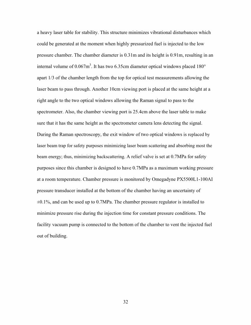
a heavy laser table for stability. This structure minimizes vibrational disturbances which
could be generated at the moment when highly pressurized fuel is injected to the low
pressure chamber. The chamber diameter is 0.31m and its height is 0.91m, resulting in an
internal volume of 0.067m3. It has two 6.35cm diameter optical windows placed 180°
apart 1/3 of the chamber length from the top for optical test measurements allowing the
laser beam to pass through. Another 10cm viewing port is placed at the same height at a
right angle to the two optical windows allowing the Raman signal to pass to the
spectrometer. Also, the chamber viewing port is 25.4cm above the laser table to make
sure that it has the same height as the spectrometer camera lens detecting the signal.
During the Raman spectroscopy, the exit window of two optical windows is replaced by
laser beam trap for safety purposes minimizing laser beam scattering and absorbing most the
beam energy; thus, minimizing backscattering. A relief valve is set at 0.7MPa for safety
purposes since this chamber is designed to have 0.7MPa as a maximum working pressure
at a room temperature. Chamber pressure is monitored by Omegadyne PX5500L1-100AI
pressure transducer installed at the bottom of the chamber having an uncertainty of
±0.1%, and can be used up to 0.7MPa. The chamber pressure regulator is installed to
minimize pressure rise during the injection time for constant pressure conditions. The
facility vacuum pump is connected to the bottom of the chamber to vent the injected fuel
out of building.
32

Instrumentation
Raman Scattering System.
A simple schematic of the instrumentation setup for the Raman spectroscopy is
shown in Figure 18. A Spectra-Physics Millenia Pro, continuous wave (CW), Nd:YVO4
laser is used as the light source producing 10 Watts at 532 nm frequency. This diode
pumped solid state laser (DPSSL) generates the vertical polarization with 2.3mm±10%
beam width. The beam is turned 90 degrees twice by two different mirrors mounted on
each side of the laser rail arm and focused after passing through a 1-meter focusing lens
placed between the two mirrors. The beam then, enters the chamber optical window and
focuses at the center of the chamber perpendicular to the direction of jet injection
allowing for one-dimensional measurements in the beam path direction.
Beam Trap
Spectrometer
+ CCD camera
Laser Rail
Mirror Lens Mirror
Lens
Viewing Window
Injection Chamber
Laser Beam
Nozzle
Laser
1-m focal Lens
x
y
Figure 18. Schematic of Raman spectroscopy instrumentation.
The exit window is replaced by the beam dump to minimize backscattering and
reflection that cause signal disruption. The scattered signal is collected by the
spectrometer. It is focused by a 58mm, f /1.2 Noct Nikon camera lens mounted on the
33

laser table just outside of 10cm viewing window at right angles to the beam path. The
Rayleigh and Mie scattering as well as stray light, is either minimized in intensity or
filtered out by the colored, 3mm thick, Schott glass OG570 long path filter before
entering the focusing camera lens. The Raman signal passing through the camera lens
then focuses on the 1mm width entrance slit. Once again, the Holographic Notch Filter is
employed to separate the Q-branch vibrational Raman signal component. The 3600
grooves/mm Holographic transmittance grating is selected to obtain the signal spectrum
throughout this research. Its wavelength range selection is only for nitrogen, methane,
and ethylene wavenumbers, (Table 2).
Each wavelength is captured by Andor’s iXonTM+, back-illuminated with 512×512
pixel array (24×24 mμ each pixel size), Electron Multiplying Charge-Coupled Device or
EMCCD detector at the focal plane. Several different binning factors are available to
perform the statistical analysis. The vertical 2×2 binning factor (total 4 pixels) is selected
for all images captured in the present research. This is because only the variation in
concentration along the laser-beam axis is of interest. Since the camera field of view is
set to view 4.2mm, the corresponding length of space viewed by each pixel is 0.016mm
along the beam axis.
The Andor software controls the CCD camera and saves captured images to the
computer as a Tagged Image File Format (TIFF or TIF) file. The camera shutter is
precisely controlled by an external trigger, Stanford Research Systems DG535 digital
delay generator, for the signal acquisition with 2 seconds of exposure. For better signal to
noise ratio (SNR), the Electron Multiplying (EM) gain is set to 75 at 223K. Ten images
are captured and averaged for the calibration and are used to determine the number
34

density. The entire spectrometer and CCD camera setup is synchronized with the laser
table, so the entire set can be traversed in the y-direction (Figure 18) to determine the jet
centerline where a maximum scattering signal is produced.
Shadowgraph Imaging System.
A direct shadowgraph technique is used to visualize the jet structure and to find
the condition where the condensation occurs. Based on that result, the desired down
stream location can be determined. The light source is a continuous wave, high pressure
mercury arc lamp providing an average brightness of 140,000 candles per square
centimeter. As can be seen in Figure 20, the pin hole aperture is placed between two
lenses to produce a point light source. The optical lens is accurately placed to collimate
the light. The two optical windows are cleaned before being placed on the chamber to
take dust free image data.
CCD Camera
Figure 20. Direct shadowgraph imaging instrumentation.
The 5cm square FGL495S 495nm frequency glass filter is used as a long pass
cutoff filter between the camera and the focusing lens to allow semi-monochromatic light
to pass through. Then, images from the injection jet are captured by the FASTCAM-
X1280 PCI high speed video camera.
Light Source Lens Glass Filter Pin Hole Aperture
35

On the CCD camera, the sharp density gradient (shock wave of the jet) and
condensation can be detected as a dark region whereas the transparent gaseous jet is
illuminated as a bright region and the corresponding image is sent to the computer. The
camera is controlled by the software installed on the computer. Images taken for the
present study are 125 frames per second with a shutter speed of 1/32000 second. The full
size, 1280×1024 pixels, and the highest sensitivity, ×8, are selected for the CCD detector.
The image file sent to the computer is stored as a TIF, one frame per file.
For this condition, the camera can capture 1024 frames for each record, hence it
can provide about 8.2 seconds recording time for each run. Tests show the injection jet
mass flow rate becomes steady about 4 seconds after injection begins. The camera can
record the entire injection process from the beginning to the end. The nozzle injection
diameter is very small, 0.5 mm. The axial distance of the Mach disk from nozzle exit
plane and the disk diameter is a few orders of magnitude larger than the injection
diameter. The camera is arranged to capture an image with a 7.3×9.1 mm field of view.
Calibration
Before calibrating the laser table and optical instruments, the chamber has to be
positioned exactly. The chamber is vertically standing with two optical viewing ports
aligned in the same direction as the laser beam path (x-direction). The center of the
viewing ports has a height of 10cm, the same height as the spectrometer camera. The
laser table is moved to level the beam path in the x-direction and to ensure the beam is at
a right angle with the second mirror.
36

Three different types of calibrations are involved to measure accurate data of each
species condensation profile. A Pen-Ray Neon lamp is used for spectral calibration
because it covers a wide spectral range and line positions are well known as shown in
Figure 21. A light ray from one side of a double-bore quartz neon tube is focused by the
camera lens and enters through a fine entrance slit with width of 0.05mm. The spectral
lines spread out along the x-axis denoting wavenumber instead of pixel numbers. Care
must be taken to locate neon lamp carefully on the laser beam path. Since the
wavenumber range of each species of interest (methane, nitrogen, ethylene) is from 5700
to 6400cm-1, the CCD camera is adjusted to cover this wavenumber range on the neon
calibration image.
As a result of spectral calibration, the CCD camera is capturing the signal of all
three species with different vibrational modes on the same image plane having the
nitrogen signal (wavenumber is 6073cm-1) at the center and the other two on the right
side of it. Also, the CCD camera has to be positioned right at the focal plane to achieve
narrow signal peaks.
Figure 21. Neon calibration image, number counts on the vertical-axis versus
wavenumber on the horizontal-axis [20].
Determining the camera’s field of view is done by imaging a razor blade. The
sharp edge of razor blade can be easily seen on the image plane. The razor blade is placed
right on the beam path near the predicted jet location in the same way as the neon lamp
37

case. The spectrometer entrance slit is set to 1mm width for this calibration. There is a
sharp change of black and white color on the focused CCD camera image where the razor
blade edge is located. Then, the razor blade is moved along the beam path to determine
where the right and left limitations are. The distance moved is the camera’s field of view
can be expressed in terms of the length of space viewed by each pixel. Based on the
previous research, the injection jet plume width itself has a size of about 30mm [5]. The
camera distance relative to the jet location is adjusted to have a suitable field of view,
4.2mm of spatial distance, each pixel is viewing 0.016mm for this study. The jet center
has to be placed right at the center of the camera field of view for achieving a symmetric
data signal.
The number density of each species can be determined by establishing the linear
relationship between the number density of each gas and the intensity of signal image
acquired by the CCD camera. This calibration was performed by filling the injection
chamber with known concentrations of nitrogen, methane, and ethylene each time.
Assuming uniform distribution, the number density inside the chamber is following the
perfect gas relation, that is
speciesspecies
species species
PR T
ρ = (12)
The chamber pressure and temperature of each gas is the same as the chamber,
those two parameters can easily be determined. The molar density, speciesC , can be
determined by the equation below:
speciesspecies
species
CMWρ
= (13)
38

where specieMW is the molecular weight of each nitrogen, methane, and ethylene which is
28.01, 16.04, 28.05 respectively [21]. Then, the number density can be founded by
species species AN C N= (14)
where is Avogadro’s number ( ). The purity of gases used for this
calibration is the same purity of the gases used for actual data acquisition, 99.95% of
nitrogen, 99.99% of methane and ethylene. The chamber is evacuated using shop air
before filling each time. It is observed 10Kpa is always left inside the chamber, however
that does not affect the signal calibration at all. As mentioned earlier, the chamber
pressure transmitter is providing ±0.1% accuracy. The background signal of ambient light
condition is taken for each gas without the laser, before taking the calibration data for the
use of background image subtraction, assuming the background intensity of the
calibration image is the same and uniform as the background intensity of ambient light
condition. However, as will be described more in the data processing section, the three
background images on its image itself is used for background subtraction, due to the
different background patterns caused by reflection, scattering and other light sources. It
has a different background intensity profile compared to the background images taken
before without the laser.
AN 236.02 10×
Before the background subtraction, it is necessary and important to select proper
signal area for calibration. After the background signal was first subtracted, selected area
of each species signal is integrated over each column pixel along the field of view, i.e. x-
axis. The least square correction method is used to determine the best line fit over each
integrated column for seven different number density cases. From the result of this
method, 256 different calibration line fits are made for each species. Overall validity of
39

these lines are above 99.4% accuracy and the calibration line constants are displayed on
Figure 22. Each line represents averaged slopes and intercepts values. The standard
deviations of those numbers are shown in Table 3.
A small number of nitrogen signal intercepts show the calibration for nitrogen is
more accurate than other species. The different slopes result from the different Raman
scattering cross section as discussed in the previous chapter. The signal intensity is
proportional to its cross section. The methane cross section of v2 is close to that of
ethylene (reference Table 2). Thus, the number density of each injecting species can be
determined from measured signals using these linear curve constants of calibration.
P R = 5352n C2H4 - 588.81
P R = 6805.7n CH4 - 372.7
P R = 1548.8n C2H4 - 165.63
P R = 718.04n N2 + 17.76
0.E+00
1.E+04
2.E+04
3.E+04
4.E+04
5.E+04
0 1 2 3 4 5 6 7 8
Normalized Number Density
Cou
nts
Ethylene I, IIEthylene IIIMethaneNitrogen
Figure 22. Calibration curve fit of Raman scattering signal.
* Ethylene I, II: v3, v2 vibrational modes, Ethylene III: v1 vibrational mode (Appendix E)
40

Table 3. Averaged calibration curve fit constants with standard deviations.
Raman Line Slope Intercept
Nitrogen 718.04 ± 43.3 17.76 ± 8.5 Methane 6805.7 ± 440.4 -372.7 ± 29.7
Ethylene I, II 1548.8 ± 123.6 -165.63 ± 13.6 Ethylene III 5352 ± 628.5 -588.81 ± 64.9
Experimental Procedure
Overview.
There are two main experimental sets. One is shadowgraph and the other is
Raman spectroscopy. Both the shadowgraph and the Raman spectroscopy are for
characterizing and determining the species distribution profile of the supercritical jet.
Since the Raman spectroscopy is sensitive to molecular species, the accumulator is
flushed out once before the initial filling of fuel to avoid the presence of unwanted gas
species. Then, the fuel is charged in one side of the accumulator and nitrogen in the other
side to control the desired supply pressure by the regulator. A methane/ethylene mixture
is prepared manually, by Dalton’s law of partial pressure. The number of moles of each
gas is the partial pressure. The desired mole fraction of methane, , can be found by 4CHX
4 44
4 2 4 4 2 4( ) ( )CH CH
CHCH C H CH C H
n P Xn n P P
=+ +
= (15)
where n is a number density and P is a partial pressure.
The chamber regulator is pre-adjusted to provide a constant pressure level during
the injection. After each injection, the 1.03Mpa shop air is on to vent the injected fuel and
nitrogen gas out of the chamber. The chamber is flushed with nitrogen once again to
41

minimize the effect on the signal by the injected fuel remaining in the chamber for the
Raman spectroscopy.
Shadowgraph.
The shadowgraph technique is relatively simple and similar to Raman
spectroscopy once the image resolution and appropriate field of view is determined. Four
different runs are performed for each nozzle, each run is corresponding to each
temperature condition. The mass flow rate of the jet becomes steady state four seconds
after injection begins. The entire image is acquired and saved to the computer. Then, 40
consecutive time-averaged images in the four second time frame are selected and
averaged for improving the image quality.
Raman scattering.
Before testing begins, the laser is set to safe mode and proper alignment between
optical set and chamber is observed at the beam off-angle. Then, the laser transition table
is moved in the positive y-axis direction to the predetermined position. Since the Raman
signal is very sensitive to light, all the unnecessary light in the laboratory is turned off. A
dark covering is provided between the collection camera lens and the entrance slit. The
spectrometer assembly is sealed off by black tape to minimize the interference of
background lighting. Three sets of runs are performed for each temperature condition
with four different nozzle configurations. After finishing four temperature conditions, the
chamber is filled with air at ambient pressure and the laser intensity is reduced back
down to safe mode. Then the chamber is closed until the nozzle is changed to another
one. Each time the nozzle is changed, the laser needs to be realignment to the center of
the jet. Assuming the jet has a circular cone shape and uniform distribution of molecules,
42

the center line is where the largest number of molecules is detected. At the centerline, the
larger number of molecules scatter the signal much more than other areas. Then, the
stronger signal intensity can be acquired on the CCD camera. Just as with the
shadowgraph, the jet becomes steady four seconds after the injection begins. The jet is
controlled to not exceed eight seconds because the accumulation of the fuel in the
chamber will affect the signal. The external trigger for the camera shutter is used to
accurately measure the jet. It is connected to the apparatus initiated by the injection valve.
The shutter is opened for two seconds and the image is viewed on the computer screen
and saved as a TIF file. Three runs are performed for the same temperature and the
intensity is averaged. Before running the jet, ten time averaged images are taken for
background signal and subtracted from the signal image to have a better signal to noise
ratio.
Testing Strategy
Test fuels for this study are pure ethylene, a mixture of ethylene and methane with
methane mole fractions of 0.1 and 0.2. As mentioned earlier, typical fuels above the
critical point start to crack down to simpler molecular species, particularly ethylene and
methane. Thus, ethylene and methane are selected. Ethylene’s critical point is near room
temperature which minimizes system safety requirements. Also 0.1 and 0.2 mixture ratios
are chosen to maintain the same test fluid as previous work. Nitrogen is used as the
ambient gas because it is inert and its properties are close to the air. Fuel critical
temperature and pressure point are calculated by the SUPERTRAPP program. The fuel
temperatures for this study are chosen near the fuel critical point, as can be seen in Table
43
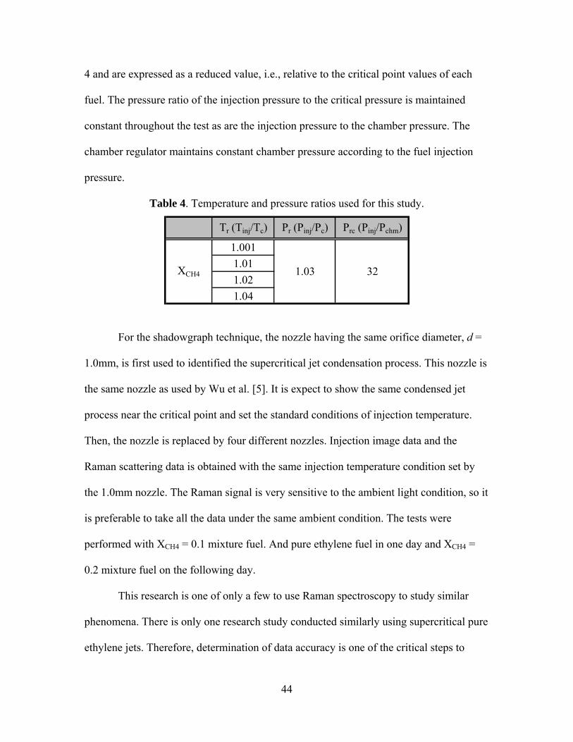
4 and are expressed as a reduced value, i.e., relative to the critical point values of each
fuel. The pressure ratio of the injection pressure to the critical pressure is maintained
constant throughout the test as are the injection pressure to the chamber pressure. The
chamber regulator maintains constant chamber pressure according to the fuel injection
pressure.
Table 4. Temperature and pressure ratios used for this study.
Tr (Tinj/Tc) Pr (Pinj/Pc) Prc (Pinj/Pchm)
1.0011.011.021.04
XCH4 1.03 32
For the shadowgraph technique, the nozzle having the same orifice diameter, d =
1.0mm, is first used to identified the supercritical jet condensation process. This nozzle is
the same nozzle as used by Wu et al. [5]. It is expect to show the same condensed jet
process near the critical point and set the standard conditions of injection temperature.
Then, the nozzle is replaced by four different nozzles. Injection image data and the
Raman scattering data is obtained with the same injection temperature condition set by
the 1.0mm nozzle. The Raman signal is very sensitive to the ambient light condition, so it
is preferable to take all the data under the same ambient condition. The tests were
performed with XCH4 = 0.1 mixture fuel. And pure ethylene fuel in one day and XCH4 =
0.2 mixture fuel on the following day.
This research is one of only a few to use Raman spectroscopy to study similar
phenomena. There is only one research study conducted similarly using supercritical pure
ethylene jets. Therefore, determination of data accuracy is one of the critical steps to
44

proof whether the resulting data is valid or not. The certified methane/ethylene mixture
gas with methane mole fraction 0.1 is used for filling up the tank with known
concentration to determine mole fraction ratio of the ethylene to the methane. If the
resulting mole fraction ratio is exactly nine, the overall data processing and calibration
are accurately done. The same data processing method can then be applied to the Raman
signal data with manually mixed fuels.
During the course of the experiment, the entire laser table is moved 5.0mm in the
negative x-axis direction to relocate the jet centerline at the center of the camera field of
view. For this reason, each species Raman signal is moved three pixels to the right along
the wavenumber axis. This could affect the background pattern. Therefore, there might be
inconsistency between the calibration data and the injection data. Also, the certified fuel
with the methane mole fraction 0.1 was not enough to cover all amount of testing. The
manually mixed fuel is used for the Raman spectroscopy. Thus, it is not sure how
accurate the mole fraction is for the mixture fuel. The only way to determine the fuel
mole fraction is taking the Raman signal data of the injection fuel after filling the
chamber with known concentrations. It can be determined using the calibration
correlation constants. The detailed results of this step are discussed on the next chapter.
Data Processing
Shadowgraph Image.
The imaging process for the shadowgraph is fairly simple and straightforward.
Entire sets of images taken during each run are stored in an external hard drive. Forty
consecutive images are averaged in terms of intensity using the Image J® program. By
45

doing so, the shock wave structure and condensation can be recognized more clearly as
seen in Figure 23 (b). The undesirable disturbances appearing in a couple of images along
with turbulent irregularity around the jet structure are either removed or minimized. The
averaged image is separated to the red, green, or blue color component. Blue color is
filtered out by the glass filter, so it does not contribute to any image information. The
green component image is selected and filtered by the custom made filter which uses Fast
Fourier Transform to refine the image. As can be identified in Figure 23, the barrel shock
structure looks clearer. The dark regions appeared on both sides of the image (c) can be
easily identified that are not clear on the first two images, (a) and (b). Generally, on the
shadowgraph image, the denser region appears as a dark region. For this image, the dark
region represents a change in density gradient. The condensed phase molecules are
represented in the gaseous phase. This kind of small condensed jet is hard to be
distinguished on the raw image. The same shadowgraph image data processing
procedures are applied throughout this research.
(a) (b) (c)
Figure 23. (a) The raw shadowgraph image data, (b) Averaged, (c) Filtered.
46

Raman Scattering Data.
The data processing of the Raman signal is relatively complicated and requires
delicate processing due to the fact that the signal and the background intensity are
sensitive to the area of selection. Any changes must be done uniformly across all images
and any artificial data manipulation to make it look aesthetically pleasing must be
avoided. Three images were taken for each test condition. The raw images of the CCD
camera were saved on the computer as a Tiff file format and the Mathcad® program is
used for the Raman scattering data processing. There are a few steps that need to be taken
to reach the final destination of determining each species concentration profile. The raw
image is a 256×256 pixel matrix containing intensity information of each species as
wavenumber on the x-axis versus field of view on the y-axis. It is rotated 90° to the right
to reorient as field of view on the x-axis as shown in the Figure 24 (a). The white line
represents the corresponding species intensity profile and the dark region is the
background signal on the image plane. Figure 24 (b) is the intensity profile along the
wavenumber, y-axis. The peaks represent ethylene I and II spikes, nitrogen, and
methane/ethylene III from the left respectively. The methane signal is hard to identify on
the image of the Figure 24 (a) due to the small amount of methane mole fraction compare
to ethylene. Although the intensity diagram of the Figure 24 (b) is showing there is a
small peak of the methane signal right before the ethylene signal peak, it is impossible to
separate the methane signal from the ethylene signal. The intensities of those species are
overlapped and mixed together. Readjusting the spectral resolution risks loosing some
species number density information because it can degrade the intensity of both gases.
47

Therefore, the method employed here is integrating methane and ethylene III line
together over the field of view and subtracting ethylene I and II intensity from it. The
methane intensity will be left and the number density can be determined from it. This
process follows the background subtraction. In addition, Figure 24 (b) is showing there is
no other foreign gas species signal appearing on the intensity diagram. Oxygen line is
supposed to be located between ethylene II and nitrogen, but it is completely removed
from the chamber by the shop air. It must be noted ethylene has three distinguishable
signal lines containing different types of vibrational information for the same ethylene
molecules. Ethylene I is at 1342frequency (H-C-H scis), ethylene II is at 1623nm
frequency from v2 vibractional mode (C=C stretching), ethylene III is at 3020nm
frequency from v1 vibractional mode (H-C-H stretching). The reason of integrating
ethylene I and II together at the same time is to increase SNR. It is found another small
methane signal line is located between the two.
Field of View
Inte
nsity
Wavenumber
Methane Peak
Ethylene II Ethylene I
Nitrogen
Methane Ethylene III
Wav
enum
ber
(a) (b)
Figure 24. (a) Raman Image, (b) Intensity profile along the y-axis.
48

Figure 25 is showing the 3-dimensional intensity diagram of the image of Figure
25(a). The intensity is on the z-axis and its profile is different along the field of view axis.
It needs to be noted relatively small signal intensity is still appearing around the ethylene
III signal even though it is not clear on the image of Figure 25 (b), this is generally the
same for all other signal lines. Thus, this kind of region must be avoided for selecting the
background image area. Also, the brightest region of the ethylene III line on the image
(Figure 24 (a)) corresponds to the peak area of intensity where the largest number density
of ethylene III species exists on the 3-D diagram. It is expected that the peak intensity
area is where the jet center is. In addition, the signal intensity deficit at the ethylene peak
is caused by CCD camera defect. It is always at that location and this deficit affects the
species mole fraction profile.
Inte
nsity
(z)
Wavenumber (y)
Field of View (x)
Figure 25. 3-D signal intensity profile by Image J® surface plot.
Subtracting appropriate background signal is the key to the success of this study
for accurate results. However, the problem is every each image has different background
49

intensity profiles making the background subtraction difficult as shown in Figure 26. It
appears as every image has the same and uniform background. However after adjusting
the brightness of the image with Image J® program, it does not have a uniform intensity
distribution on the background area. This irregular background is caused by the reflecting
from internal structure of the chamber and the window of viewing port. It is expected also
the signal line is affected by this back scattering too. It is also observed every image has
different background intensity and the intensity profile is different from the area of
selection on the same image itself. It tends to proportionally increase as the signal
intensity increases for the calibration image data. Therefore, the image taken for
background signal is no more useful because it has a uniform intensity. The appropriate
background signal has to be selected and subtracted from both calibration and injection
data processing consistently.
Three background images are taken from its own image data. The area between
the signal lines are selected and averaged along the field of view axis and subtracted from
the image data. Figure 26 shows how the background intensity profile varies along the x-
axis as well as y-axis. Care must be provided to select the background image which
contains the closest intensity profile to the signal line, while also avoiding the signal line.
Once the background area is determined, the same area is used for background image
subtraction for all the data images throughout the processing for consistency. For this
study, the areas between ethylene II and oxygen, oxygen and nitrogen, nitrogen and
methane/ethylene III lines are selected. Each area of selection has seven rows. Those
areas are integrated over field of the view axis and averaged to give a single line intensity
profile.
50
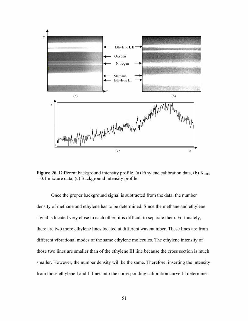
Figure 26. Different background intensity profile. (a) Ethylene calibration data, (b) XCH4 = 0.1 mixture data, (c) Background intensity profile.
Once the proper background signal is subtracted from the data, the number
density of methane and ethylene has to be determined. Since the methane and ethylene
signal is located very close to each other, it is difficult to separate them. Fortunately,
there are two more ethylene lines located at different wavenumber. These lines are from
different vibrational modes of the same ethylene molecules. The ethylene intensity of
those two lines are smaller than of the ethylene III line because the cross section is much
smaller. However, the number density will be the same. Therefore, inserting the intensity
from those ethylene I and II lines into the corresponding calibration curve fit determines
Ethylene I, II
Nitrogen
Oxygen
(a) (b)
y
Ethylene III Methane
x
(c)
z
x
51

the ethylene number density, which is eventually the same number as the ethylene line
close to the methane signal. The equation for determining ethylene number density is:
2 4 2 4RC H C HP an b= + (16)
where a and b are coefficients of the corresponding calibration line and PR and ni are
number density and intensity, respectively. The next step is to insert this number density
into the calibration curve fit of the ethylene III signal to determine the intensity. The
integration of the main ethylene and methane signal produces the total intensity of
ethylene and methane. Subtracting off the ethylene III intensity determined by its own
calibration curve from the total intensity gives just the methane intensity itself. Finally,
the methane number density can be determined by inserting the methane intensity into its
own calibration curve fit. Consequently, the methane and ethylene number density are
determined individually and the mole fractions of each gas can be derived from the
number density.
The exact same manner is applied to the nitrogen signal; integration over the field
of view axis to determine the intensity profile. The nitrogen number density can be
determined by inserting the intensity profile into its own calibration curve fit.
52

IV. Results and Discussion
Chapter Overview
The main purposes of the shadowgraph images are the identification of the jet
global appearance and finding the jet condensation condition in terms of injection
temperature. The previous research explored the injection temperature effects on the
supercritical jet condensation process. The near-field jet characteristics are well discussed
in terms of axial location and size of the Mach disk and expansion angle. Therefore, it is
not necessary to repeat the whole process in this study, but the same procedure is
repeated to find the jet condensation condition which might be slightly different from the
previous work since a smaller nozzle diameter is used. The nozzle with the same nozzle
diameter is used to compare the difference between a smaller nozzle diameter and the
previous work. The shadowgraph image results for the different nozzles are compared to
identify the nozzle design effects on the jet shape and condensation. The Raman
scattering technique is employed at the jet down stream location to determine molecular
profiles.
The mole fraction of ethylene, methane, and nitrogen at different injection
temperature conditions are studied to identify the condensation effects on the fuel mixing
process with the air (nitrogen in this study). The mole fraction ratio of ethylene to
methane for each fuel condition is also studied to clarify whether there is any preferential
condensation within the jet. In addition, each species mole fraction for the different
nozzles is compared to determine which nozzle design is better than another in terms of
mixing characteristics, which is the fast spreading rate. Those three main themes are the
main discussion points. The methane’s signal to noise ratio (SNR) is relatively lower than
53

ethylene and nitrogen due to its small mole fraction, significantly adding uncertainty to
the results. Therefore, the main discussion will be on the ethylene and the nitrogen signal
data. In addition, each nozzle’s potential core length is computed using the relation
provided by Chehroudi et al. for characterizing the jet (Chapter II).
This chapter begins with the discussion of the shadowgraph results over various
temperature range and different nozzles. It will be followed by the Raman scattering
results discussion in terms of ethylene mole fraction and mole fraction ratio of
ethylene/methane. Both the shadowgraph and the Raman scattering result are presented in
the order of supercritical ethylene, XCH4 = 0.2, 0.1 mixture fuel. Also, it needs to be noted
that a lot of discussions presented in this chapter are the comparison to the previous work
done by Wu et al. [5]. The jet divergence angle and potential core length are also
discussed to identify nozzle and condensation effects.
Shadowgraph Results Supercritical Ethylene Fuel Injection. Figure 27 is showing the actual injection condition with the injection temperature
ratio (Tr = Tinj/Tc) versus injection pressure ratio (Pr = Pinj/Pc) for each nozzle. These data
points are taken at four second after injection begins. All the injection conditions are in
the supercritical region, although there are variations due to the system inaccuracy.
Generally, the injection pressure ratio is maintained at a constant for all the cases varying
within 0.01 pressure ratio range. The injection temperature ratios are varied also from
1.01 to 1.04 which are well agree with the ratio values of the testing strategy. For nozzle
#8, three runs are conducted with Tr = 1.01, 1.04, 1.08 for the comparison to the previous
54

work done by Wu et al. [5]. The pressure ratio of the injection pressure to the chamber
(Prc = Pinj/Pchm) is maintained a constant, Prc = 30, although this is not shown in Figure 27.
0.991
1.011.021.031.041.051.061.071.081.09
1.1
1 1.01 1.02 1.03 1.04 1.05Pr
T r
Nozzle #1Nozzle #6Nozzle #7Nozzle #9Nozzle #8
Figure 27. Shadowgraph image injection condition, ethylene fuel.
Generally, a lot of condensation is observed as the injection temperature
approaches the critical temperature. Figure 29 is showing the condensed jet shadowgraph
image with d = 1.0mm nozzle at Tr = 1.01, Pr = 1.01 condition. The dark region is
considered a condensed jet since the density of the liquid phase is higher than gaseous
phase. According to Wu et al, the barrel shock is still formed inside the condensed jet, but
it is hard to recognize. It is obvious as the injection temperature increases shown in
Figure 29. The increased injection temperature does not produced as much condensed jet
as the previous case. As shown in Figure 29, less condensation is observed at Tr = 1.04, Pr
= 1.01 injection condition, but there is still small amount of condensed jet around the
barrel shock structure. The barrel shock is formed because this is a supersonic jet and an
under expanded shock structure forms. As the injection temperature moves further away
to Tr = 1.08, the jet becomes transparent. This is predicted trend based on the entropy-
55

pressure diagram as shown in Figure 4 in chapter II. Since the supercritical injection jet is
considered isentropic expansion process, as the injection temperature is approached the
critical temperature point, it enters the two phase region (liquid and vapor) which is
depicted in the same Figure 5 of chapter II. However, as the injection temperature
increases and moves away from the critical temperature, the injection process enters the
vapor regime. There is no condensed jet in this region. The shadowgraph result of nozzle
#8 shows as the injection temperature increases the condensation is less significant. This
result is well agreed with the result of previous study done by Wu et al. [5].
In addition, the Mach disk size and the jet plume are bigger than those of the
smaller nozzle diameter. The bigger nozzle diameter produces larger mass flow rates
which is proportional to the nozzle diameter. The condensed jet does not appear at Tr =
1.08, therefore the injection temperature ratio for the rest of the research is focused on the
very near critical temperature point; Tr = 1.00, 1.01, 1.02, 1.04. The first case of injection
temperature ratio case, Tr = 1.00, is rounded off number. The actual value is greater than
Tr = 1.00, but very close to it. It needs to be noted the triangle pattern in the jet plume is
not shock structure, it is the background pattern caused by the chamber optical windows.
It must be noted that the injection jet shows isentropic expansion (barrel shape
shock structure) and after that it is no more isentropic expansion. Also, the jet is not in
the supercritical condition at z/d = 100 location.
56

Figure 28. Shadowgraph image, ethylene, nozzle #8, d = 1mm, Tr = 1.01, Pr = 1.01
Figure 29. Shadowgraph image, ethylene, nozzle #8, d = 1mm, Tr = 1.04, Pr = 1.01
57

Figure 30. Shadowgraph image, ethylene, nozzle #8, d = 1mm, Tr = 1.08, Pr = 1.02 Four nozzles with a small nozzle diameter (d = 0.5mm) are used to study the
condensation process, whether it occurs the same way or not, as well as whether any
particular condensation is observed depending on the nozzle configuration. The fuel
critical temperature and pressure point are different from those of pure ethylene.
However, the injection pressure ratio remained at the same value as nozzle #8. Each
nozzle has four different injection temperature ratios; 1.00, 1.01, 1.02, 1.03. The chamber
pressure ratio also maintains a constant value of Prc = 30.
The same jet condensation process is observed throughout the different injection
temperatures and nozzles. The barrel shock size is smaller than for the nozzle #8 cases
due to the smaller nozzle diameter (mass flow rate). Also, the amount of condensation is
58

slightly reduced comparing to the nozzle #8 cases. Figure 31 and 35 show the
condensations are occurring at the outer edge of the barrel shock.
Nozzle #6 is producing a relatively small amount of condensation on both sides
of the barrel shock. Most of the shadowgraph image is showing the jet has a symmetrical
shape. In addition, as the injection temperature increases the condensation is hard to
identify. There might still be a very small amount of condensation where still noticeable
amounts of condensation are produced in the same case of nozzle #8, Figure 29.
59

Figure 31. Shadowgraph image, ethylene, Nozzle #1, d = 0.5mm, Tr = 1.00, Pr = 1.03
Figure 32. Shadowgraph image, ethylene, nozzle #1, d = 0.5mm, Tr = 1.01, Pr = 1.03
60

Figure 33. Shadowgraph image, ethylene, nozzle #1, d = 0.5mm, Tr = 1.02, Pr = 1.03
Figure 34. Shadowgraph image, ethylene, nozzle #1, d = 0.5mm, Tr = 1.03, Pr = 1.03
61

Figure 35. Shadowgraph image, ethylene, nozzle #6, d = 0.5mm, Tr = 1.00 Pr = 1.04
Figure 36. Shadowgraph image, ethylene, nozzle #6, d = 0.5mm, Tr = 1.01 Pr = 1.03
62
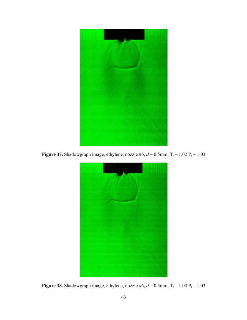
Figure 37. Shadowgraph image, ethylene, nozzle #6, d = 0.5mm, Tr = 1.02 Pr = 1.03
Figure 38. Shadowgraph image, ethylene, nozzle #6, d = 0.5mm, Tr = 1.03 Pr = 1.03
63

Figure 39. Shadowgraph image, ethylene, nozzle #7, d = 0.5mm, Tr = 1.00 Pr = 1.02
Figure 40. Shadowgraph image, ethylene, nozzle #7, d = 0.5mm, Tr = 1.01, Pr = 1.03
64

Figure 41. Shadowgraph image, ethylene, nozzle #7, d = 0.5mm, Tr = 1.02, Pr = 1.03
Figure 42. Shadowgraph image, ethylene, nozzle #7, d = 0.5mm, Tr = 1.03, Pr = 1.03
65

Figure 43. Shadowgraph image, ethylene, nozzle #9, d = 0.5mm, Tr = 1.00, Pr = 1.03
Figure 44. Shadowgraph image, ethylene, nozzle #9, d = 0.5mm, Tr = 1.01 Pr = 1.03
66

Figure 45. Shadowgraph image, ethylene, nozzle #9, d = 0.5mm, Tr = 1.02 Pr = 1.03
Figure 46. Shadowgraph image, ethylene, nozzle #9, d = 0.5mm, Tr = 1.04 Pr = 1.02
67

Supercritical Methane and Ethylene Mixture (XCH4 = 0.1 ) Fuel Jet. The same injection condition is maintained fro these test cases, while the injection
pressure ratio is a little bit higher than the ethylene injection. The pressure ratio of nozzle
#9 and nozzle #7 are lower than others. This is because the fuel supply is limited. But, all
the injection conditions are inside the supercritical region.
Also, the same result is observed. An asymmetric condensed jet is produced
possibly caused by injection tube machining irregularities.
1
1.01
1.02
1.03
1.04
1.05
1.06
1 1.01 1.02 1.03 1.04 1.05
Pr
T r
Nozzle #1Nozzle #6Nozzle #7Nozzle #9
Figure 47. Shadowgraph image injection conditions, XCH4 = 0.1 mixture fuel.
68

Figure 48. Shadowgraph image, XCH4 = 0.1, nozzle #1, d = 0.5mm, Tr = 1.00, Pr = 1.04
Figure 49. Shadowgraph image, XCH4 = 0.1, nozzle #1, d = 0.5mm, Tr = 1.01, Pr = 1.04
69

Figure 50. Shadowgraph image, XCH4 = 0.1, nozzle #1, d = 0.5mm, Tr = 1.02, Pr = 1.04
Figure 51. Shadowgraph image, XCH4 = 0.1, nozzle #1, d = 0.5mm, Tr = 1.04, Pr = 1.04
70

Figure 52. Shadowgraph image, XCH4 = 0.1, nozzle #6, d = 0.5mm, Tr = 1.00, Pr = 1.04
Figure 53. Shadowgraph image, XCH4 = 0.1, nozzle #6, d = 0.5mm, Tr = 1.01, Pr = 1.04
71

Figure 54. Shadowgraph image, XCH4 = 0.1, nzzle #6, d = 0.5mm, Tr = 1.02, Pr = 1.03
Figure 55. Shadowgraph image, XCH4 = 0.1, nozzle #6, d = 0.5mm, Tr = 1.04, Pr = 1.03
72

Figure 56. Shadowgraph image, XCH4 = 0.1, nozzle #7, d = 0.5mm, Tr = 1.00, Pr = 1.01
Figure 57. Shadowgraph image, XCH4 = 0.1, nozzle #7, d = 0.5mm, Tr = 1.01, Pr = 1.04
73

Figure 58. Shadowgraph image, XCH4 = 0.1, nozzle #7, d = 0.5mm, Tr = 1.03, Pr = 1.04
Figure 59. Shadowgraph image, XCH4 = 0.1, nozzle #7, d = 0.5mm, Tr = 1.04, Pr = 1.03
74

Figure 60. Shadowgraph image, XCH4 = 0.1, nozzle #9, d = 0.5mm, Tr = 1.00, Pr = 1.04
Figure 61. Shadowgraph image, XCH4 = 0.1, nozzle #9, d = 0.5mm, Tr = 1.01, Pr = 1.01
75

Figure 62. Shadowgraph image, XCH4 = 0.1, nozzle #9, d = 0.5mm, Tr = 1.03, Pr = 1.04
Figure 63. Shadowgraph image, XCH4 = 0.1, nozzle #7, d = 0.5mm, Tr = 1.04, Pr = 1.03
76

Raman Scattering Results
Molecular concentration profiles of nitrogen, methane and ethylene at a z/d = 100
downstream location are measured using the Raman scattering. Three different fuels are
used. Pure ethylene jet species profiles are first compared to the previous study done by
Wu et al. [5]. The XCH4 = 0.1 and 0.2 mixture concentration profiles of different nozzles
and injection temperatures will be discussed. Figure 64 shows the overall data processing
accuracy. The movement of the laser table is expected to cause some inconsistency
between the calibration and injection data. The blue line of Figure 64 is the mole fraction
ratio of ethylene to methane determined from the number density of each gas for the
certified gas with XCH4 = 0.1.
The actual methane concentration is 10.378 ± 0.02 of error, thus the expected
mole fraction ratio is 8.636 based on the certification document. The averaged mole
fraction of data processing is 8.736 ± 0.113. The average value and standard deviation
value is calculated from five different pressure cases. This result is proving the data
processing method is very accurately performed and both mole fraction ratios agree well
with each other. Although the intercept values of the calibration data curve fits are not
quite zero, the calibration constants provide accurate and consistent measurement. The
XCH4 = 0.1 mixture fuel data was taken before moving the laser table. Thus, it is
necessary to check the mole fraction ratio of the fuel used for the actual Raman signal
data.
The red line on Figure 64 is representing the mole fraction ratio of XCH4 = 0.2
mixture fuel. This fuel is not certified gas. Instead it is manually mixed fuel using the
accumulator. Therefore, the accuracy of the methane gas mole fraction is not known.
77

However, the data results show the mole fraction ratio of ethylene to methane is close to
four.
The average mole fraction ratio value is 3.444 ± 0.150. Based on this number, the
calculated methane concentration is 22.522%. Those two mixed fuel mole fraction ratio is
almost constant along the field of view axis, but the right side of XCH4 = 0.2 mixture fuel
is higher than left side. This slight variation will largely affect to methane mole fraction
due to the small amount of methane concentration.
2.53
3.54
4.55
5.56
6.57
7.58
8.59
9.510
0 5 10 15 20 25 30 35 40 45Field of View (mm)
Rat
io XCH4 = 0.1XCH4 = 0.2
Figure 64. Ethylene to methane mole fraction ratio of XCH4 = 0.1, 0.2 mixture fuel without injection.
Supercritical Ethylene Fuel Injection.
Figure 65 shows the actual injection condition measured at the nozzle holder. The
values are expressed in reduced values showing all conditions in the supercritical region.
The pressure ratio of Tr = 1.00 is lower than the others simply because the fuel supply
pressure was lowered. This is not related to the condensation issue. The pressure ratio of
78

the injection to the critical pressure is generally maintained constant. In addition, the ratio
of the injection pressure to the chamber pressure is also maintained at a constant value,
although it is not specifically shown in the figure. The average increase of the chamber
pressure is 17Kpa, a small change compared to the injection pressure.
11.011.021.031.041.051.06
1 1.01 1.02 1.03 1.04 1.05
Pr
Tr
11.011.021.04
Figure 65. Raman scattering injection conditions, ethylene fuel.
The mole fractions of ethylene and nitrogen are shown in Figure 66 and Figure
69. Ethylene mole fractions shown here are calculated as:
2 4 2 42 4
2 4 4 2
C H C H bC H
C H CH N
n nX
n n n−
=+ +
(17)
where nC2H4b is the ethylene number density accumulated inside the chamber before data
collection. Other presented mole fraction values do not subtract the accumulated number
density. As an example, the ethylene mole fraction without subtraction is presented in
Figure 66. The nitrogen and methane mole fractions are actually calculated as:
2( 4)2( 4)
2 4 4 2
N CHN CH
C H CH N
nX
n n n=
+ + (18)
79

The sum of the species mole fractions are one. The data points of each line
represent the average value of three tests for the same condition and the error bar is the
standard deviation of them.
As identified in Figure 66, the ethylene centerline mole fraction peak value
decreases as the temperature ratio increases from 1.00 to 1.04. Based on the shadowgraph
results, a condensed jet is observed close to the critical temperature. The condensation
becomes less significant as the injection temperature increases above the critical
temperature point. Thus, the higher mole fraction is caused by the fuel condensation
process and the condensed jet is not mixed well with the air compared to other jets at
higher injection temperature condition.
Previous research measured the jet width at the stoichiometric level of 0.065 and
reported the jet width decreased 14mm to 13mm as the injection temperature ratio
increases from 1.04 to 1.27 [5]. In this study, the jet width is calculated using full width
half maximum (FWHM). The resulting jet width is 11.8mm for Tr = 1.00 and 11.9mm for
Tr = 1.04. The jet width in this study is smaller than previous work done by Wu et al. [5],
because the nozzle diameter of previous work is 1mm. Also, the jet width is almost
constant value over the different injection temperatures in this study. This could be the
result of the narrow temperature rage of this study. The temperature range of the previous
study is from 294K to 354K compared to the 282K to 294K for this study. Therefore, the
width appears as a constant value for this study.
The jet center value of ethylene mole fraction calculated by Wu et al. [5] at Tr =
1.04 is, XCL = 0.2, higher than that (XCL = 0.16) of 0.5mm diameter nozzle in this study.
This difference is because of the different mass flow rate. The mass flow rate reported on
80

the previous paper was 12.1g/s at that particular temperature condition. The measured
mass flow rate is 3.6g/s in this study. The mass flow rate is proportional to nozzle
diameter. The bigger nozzle produces larger mass flow rates than the smaller nozzle does.
The ethylene mole fraction is divided by its centerline mole fraction to compare it
to Wu et al. [5]. The previous study employs a pseudo-diameter approach to determine
centerline mole fraction value and normalize the measured mole fraction to check the
self-similar characteristics for the different injection temperature case [5]. But, there is
10% difference between pseudo-diameter centerline mole fraction and measured
centerline mole fraction at the temperature close to the critical point. This is caused by
condensation. However, the pseudo-diameter centerline mole fraction value agrees well
with other temperature conditions where the condensation becomes less [5].
In this study, the ethylene mole fraction is divided by its own centerline mole
fraction value without calculating pseudo-diameter centerline mole fraction. The
calculation requires additional values not measured for this study (specific heat ratio).
The radial ethylene mole fraction profile normalized by the centerline value is shown in
Figure 68. All the curves collapse onto a single curve and can be modeled by the best
curve fit:
2
2exp7.2CL
X yX
⎛= −⎜
⎝ ⎠
⎞⎟ (19)
The previous curve fit is also presented on the same Figure 68 showing the jet
width is narrower than for this study. Overall, the result agrees well with previous
research in terms of mole fraction profile and temperature effects on the mole fraction
values, although each value is not quite matched each other.
81

0
0.05
0.1
0.15
0.2
0.25
0.3
0.35
0.4
0 5 10 15 20 25 30 35 40 45Field of View (mm)
Mol
e Fr
actio
nTr = 1.00Tr = 1.01Tr = 1.02Tr = 1.04
Figure 66. Ethylene mole fraction, ethylene, nozzle #1.
0
0.02
0.04
0.06
0.08
0.1
0.12
0.14
0.16
0.18
0.2
0 5 10 15 20 25 30 35 40 45
Field of View (mm)
Mol
e Fr
actio
n
Tr = 1.00Tr = 1.01Tr = 1.02Tr = 1.04
Figure 67. Ethylene mole fraction, ethylene, nozzle #1, without accumulated number density.
82

0
0.2
0.4
0.6
0.8
1
1.2
0 5 10 15 20 25 30 35 40 45
Field of View (mm)
Mol
e Fr
actio
nTr = 1.00Tr = 1.01Tr = 1.02Tr = 1.04Curve FitWu et al.[5]
Figure 68. Normalized ethylene mole fraction, ethylene, nozzle #1.
0.5
0.6
0.7
0.8
0.9
0 5 10 15 20 25 30 35 40 45
Field of View (mm)
Mol
e Fr
actio
n
Tr = 1Tr = 1.01Tr = 1.02Tr = 1.04
Figure 69. Nitrogen mole fraction, ethylene, nozzle #1.
83
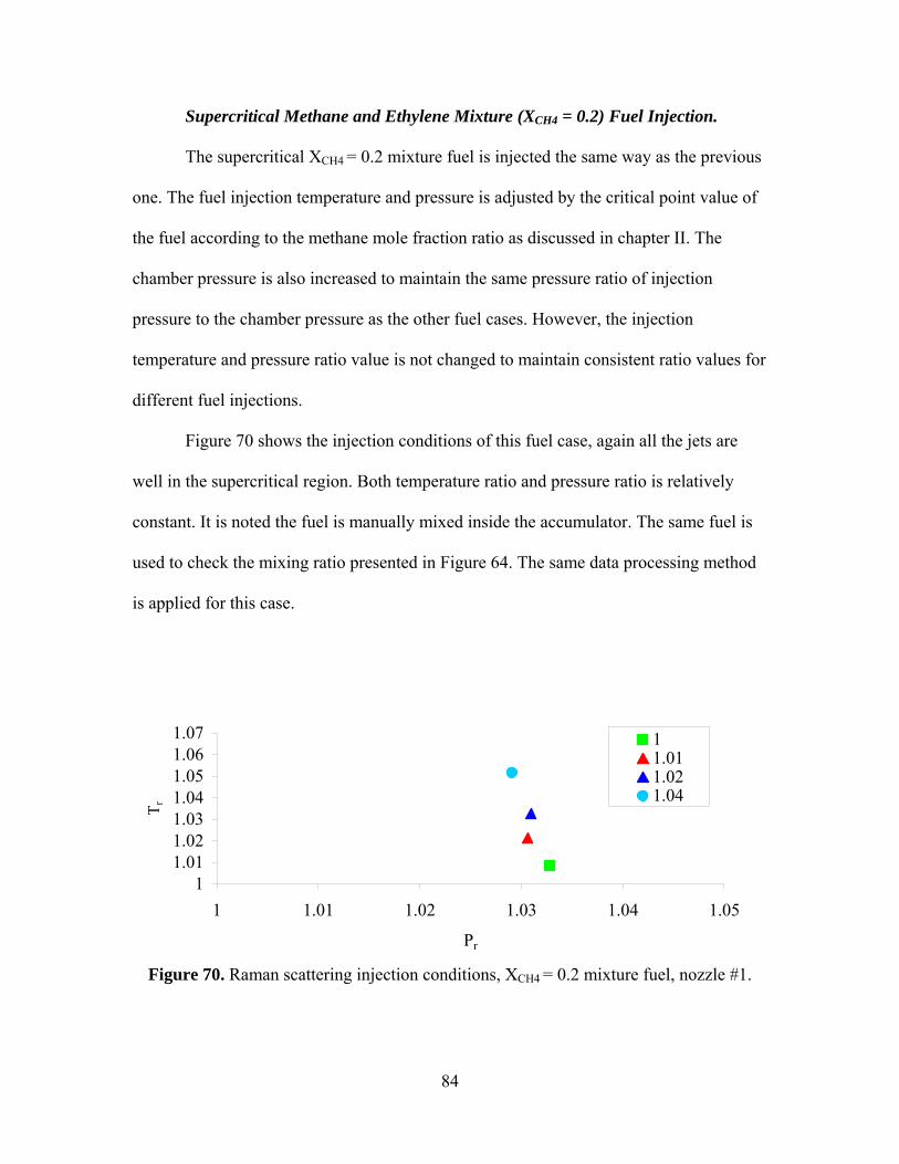
Supercritical Methane and Ethylene Mixture (XCH4 = 0.2) Fuel Injection.
The supercritical XCH4 = 0.2 mixture fuel is injected the same way as the previous
one. The fuel injection temperature and pressure is adjusted by the critical point value of
the fuel according to the methane mole fraction ratio as discussed in chapter II. The
chamber pressure is also increased to maintain the same pressure ratio of injection
pressure to the chamber pressure as the other fuel cases. However, the injection
temperature and pressure ratio value is not changed to maintain consistent ratio values for
different fuel injections.
Figure 70 shows the injection conditions of this fuel case, again all the jets are
well in the supercritical region. Both temperature ratio and pressure ratio is relatively
constant. It is noted the fuel is manually mixed inside the accumulator. The same fuel is
used to check the mixing ratio presented in Figure 64. The same data processing method
is applied for this case.
11.011.021.031.041.051.061.07
1 1.01 1.02 1.03 1.04 1.05
Pr
T r
11.011.021.04
Figure 70. Raman scattering injection conditions, XCH4 = 0.2 mixture fuel, nozzle #1.
84

The ethylene mole fraction at the centerline of the Figure 71 and Figure 72
decreases compared to the previous case. That is also because of the small mass flow
rate. The measured average mass flow rate value is 3.08g/s in this case. The condensed
jet has the highest value of centerline mole fraction. It mixes relatively poorly mix,
slowly spreading out into the nitrogen.
The lower mole fraction indicates better mixing with the nitrogen. Therefore,
injection of the condensed jet is less preferred from a fuel mixing perspective. The
higher nitrogen mole fraction shows better mixing, and the nitrogen mole fraction of
condensed jet has the lowest number. The normalized ethylene mole fraction curve for
different injection temperatures also collapses into a single curve. The curve fit
denominator is 7.2, slightly smaller than for the ethylene jet.
0
0.05
0.1
0.15
0.2
0.25
0.3
0.35
0 5 10 15 20 25 30 35 40
Field of View (mm)
Mol
e Fr
actio
n
Tr = 1.00Tr = 1.01Tr = 1.02Tr = 1.04
Figure 71. Ethylene mole fraction, XCH4 = 0.2 mixture, nozzle #1.
85

0
0.02
0.04
0.06
0.08
0.1
0.12
0.14
0.16
0 5 10 15 20 25 30 35 40 45
Field of View (mm)
Mol
e Fr
actio
nTr = 1.00Tr = 1.01Tr = 1.02Tr = 1.04
Figure 72. Ethylene mole fraction, XCH4 = 0.2 mixture, nozzle #1, without accumulated number density.
0
0.1
0.2
0.3
0.4
0.5
0.6
0.7
0.8
0.9
1
1.1
1.2
0 5 10 15 20 25 30 35 40 45Field of View (mm)
Mol
e Fr
actio
n
Tr = 1.00Tr = 1.01Tr = 1.02Tr = 1.04Curve Fit
Figure 73. Normalized ethylene mole fraction, XCH4 = 0.2 mixture, nozzle #1.
86

0
0.02
0.04
0.06
0.08
0.1
0 5 10 15 20 25 30 35 40 45
Field of View (mm)
Mol
e Fr
actio
n
Tr = 1.00Tr = 1.01Tr = 1.02Tr = 1.04Gaussian Fit
Figure 74. Methane mole fraction, XCH4 = 0.2 mixture, nozzle #1.
0.5
0.55
0.6
0.65
0.7
0.75
0.8
0.85
0.9
0.95
1
0 5 10 15 20 25 30 35 40 45
Field of View (mm)
Mol
e Fr
actio
n
Tr = 1Tr = 1.01Tr = 1.02Tr = 1.04
Figure 75. Nitrogen mole fraction, XCH4 = 0.2 mixture, nozzle #1.
87
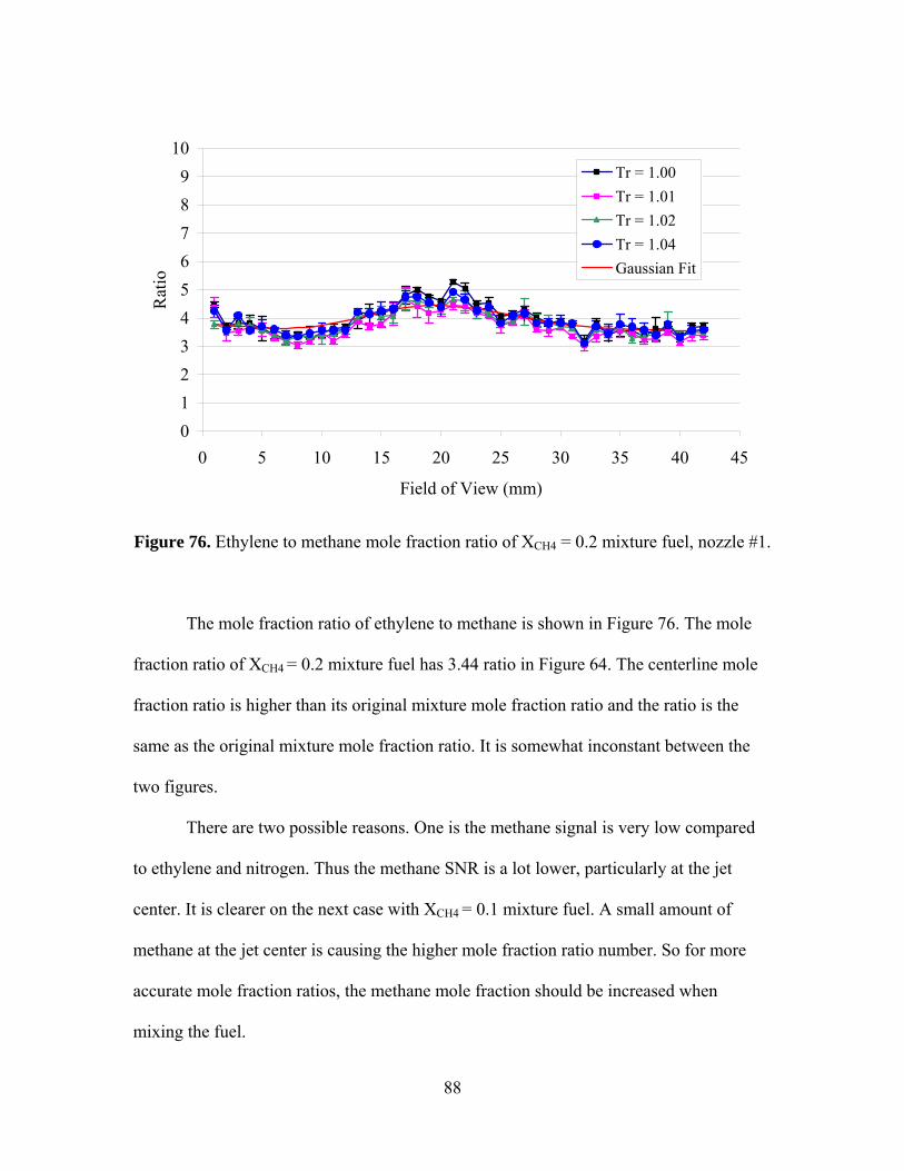
0123456789
10
0 5 10 15 20 25 30 35 40 45
Field of View (mm)
Rat
ioTr = 1.00Tr = 1.01Tr = 1.02Tr = 1.04Gaussian Fit
Figure 76. Ethylene to methane mole fraction ratio of XCH4 = 0.2 mixture fuel, nozzle #1.
The mole fraction ratio of ethylene to methane is shown in Figure 76. The mole
fraction ratio of XCH4 = 0.2 mixture fuel has 3.44 ratio in Figure 64. The centerline mole
fraction ratio is higher than its original mixture mole fraction ratio and the ratio is the
same as the original mixture mole fraction ratio. It is somewhat inconstant between the
two figures.
There are two possible reasons. One is the methane signal is very low compared
to ethylene and nitrogen. Thus the methane SNR is a lot lower, particularly at the jet
center. It is clearer on the next case with XCH4 = 0.1 mixture fuel. A small amount of
methane at the jet center is causing the higher mole fraction ratio number. So for more
accurate mole fraction ratios, the methane mole fraction should be increased when
mixing the fuel.
88

The other possible reason is a turbulent flow effect. At the jet centerline of the
nozzle exit plane, only ethylene and methane molecules will be detected with an initial
mole fraction ratio, for this case it should be at 4. As it progresses further and further
downstream, it is dispersed into the nitrogen environment, and the initial mole fraction
ratio is no more maintained, because of two species different dispersion rates. The
density of the jet centerline is smaller than of the nozzle exit plane but still higher than
the ambient density. Therefore, the molecular mean free path is relatively short and the
chance of collision between the ethylene and the methane molecules are high. Although
the collision probability between the ethylene molecule themselves are much higher than
the ethylene and the methane, the methane molecules can spread out faster than ethylene
from the jet centerline. Because the methane kinetic energy is smaller than ethylene, the
methane is easily bounced off from the ethylene gas molecule when two molecules
collide each other. Once the methane is spread out from the jet center, it is overwhelmed
by the turbulent flow. In this region, the gas molecule number density is fairly low and
mean free path is long enough to mix well. In addition, the data is taken four seconds
after the injection, there are a number of molecules already accumulated and mixed by
the turbulent flow. That makes the mole fraction ratio at the jet edge the same as the
original mixing ratio.
In short, the methane is spread out faster than the ethylene gas at the jet center.
And as it moves to the jet edge it is overwhelmed by the turbulent flow forcing three
gases are mixed. The data is taken after the fuel molecules are well mixed and
accumulated at the jet edge. Therefore, the centerline mole fraction ratio is higher than at
the jet edge.
89

Supercritical Methane and Ethylene Mixture (XCH4 = 0.1) Fuel Injection.
The supercritical XCH4 = 0.1 mixture of methane and ethylene fuel is injected with
the same condition as the previous two cases. Figure 77 is showing the injection
condition and the each injection temperature ratio. Again, all the injection conditions are
in the supercritical region.
11.0051.01
1.0151.02
1.0251.03
1.0351.04
1.0451.05
1 1.01 1.02 1.03 1.04 1.05
Pr
T r
Nozzle #1Nozzle #6Nozzle #7Nozzle #9
Figure 77. Raman scattering injection conditions, XCH4 = 0.1 mixture fuel.
This section has a lot more data than the other injection conditions. Four different
nozzles are used instead of one. Most of the research objectives will be discussed with
these cases. The following figures are arranged in the following order; ethylene mole
fractions for different nozzles, ethylene mole fractions for different nozzles without
accumulated ethylene number density during data acquisition, normalized ethylene mole
fractions, ethylene mole fractions for different injection temperatures for nozzle
90

comparing purpose, methane and nitrogen mole fractions for different nozzles, ethylene
and methane mole fraction ratios for different nozzles.
Ethylene Mole Fractions for Different Nozzles.
Again, the first four ethylene figures represent the ethylene mole fraction without
subtracting accumulated number density to capture the total mole fractions of unity
adding those of methane and nitrogen together. However, it is necessary to use the mole
fraction without accumulated number density to determine the differences between
condensed jets and less condensed jets. Generally, the ethylene molecules are still
concentrated at the center of the jet at the downstream location shown in Figure 78
through Figure 81. The peak value is located at the jet center for all the different nozzles
and injection cases although the values vary over the nozzles.
The condensed jet centerline mole fraction values are always higher than the
different nozzles shown in Figure 82 through Figure 85. It demonstrates the ethylene
molecules in condensed phase do not spread out fast compared to less condensed jet
cases. In other words, the condensed ethylene molecules do not mix well with the
nitrogen. That is undesired state from a combustion point of view. The nitrogen mole
fractions shown in Figure 100 through 103 are showing the nitrogen mole fraction profile
of the condensed jet case has a larger jet width as well as a lower mole fraction value at
the centerline. This means the nitrogen number density at the condensed jet centerline is
lower than others. A small number of nitrogen molecule presence means less mixing.
Therefore, the condensed phase of an ethylene jet is affecting mixing rate and is not a
desirable state inside the combustor. In addition, the ethylene mole fraction profile shape
91

is somewhat different depending on each nozzle, detailed discussion will be in the nozzle
comparison section.
0.16
0.21
0.26
0.31
0.36
0.41
0 5 10 15 20 25 30 35 40 45
Field of View (mm)
Mol
e Fr
actio
n
Tr = 1.00Tr = 1.01Tr = 1.02Tr = 1.04
Figure 78. Ethylene mole fraction, XCH4 = 0.1 mixture, nozzle #1.
0.16
0.21
0.26
0.31
0.36
0.41
0 5 10 15 20 25 30 35 40 45
Field of View (mm)
Mol
e Fr
actio
n
Tr = 1.00Tr = 1.01Tr = 1.02Tr = 1.04
Figure 79. Ethylene mole fraction, XCH4 = 0.1 mixture, nozzle #6.
92

0.16
0.21
0.26
0.31
0.36
0.41
0 5 10 15 20 25 30 35 40 45
Field of View (mm)
Mol
e Fr
actio
nTr = 1.00Tr = 1.01Tr = 1.02Tr = 1.04
Figure 80. Ethylene mole fraction, XCH4 = 0.1 mixture, nozzle #7.
0.16
0.21
0.26
0.31
0.36
0.41
0 5 10 15 20 25 30 35 40
Field of View (mm)
Mol
e Fr
actio
n
Tr = 1.00Tr = 1.01Tr = 1.02Tr = 1.04
Figure 81. Ethylene mole fraction, XCH4 = 0.1 mixture, nozzle #9.
93

0
0.05
0.1
0.15
0.2
0.25
0 5 10 15 20 25 30 35 40 45
Field of View (mm)
Mol
e Fr
actio
n
Tr = 1.00Tr = 1.01Tr = 1.02Tr = 1.04
Figure 82. Ethylene mole fraction, XCH4 = 0.1 mixture, nozzle #1, without accumulated number density.
0
0.05
0.1
0.15
0.2
0.25
0 5 10 15 20 25 30 35 40 45
Field of View (mm)
Mol
e Fr
actio
n
Tr = 1.00Tr = 1.01Tr = 1.02Tr = 1.04
Figure 83. Ethylene mole fraction, XCH4 = 0.1 mixture, nozzle #6, without accumulated number density.
94

0
0.05
0.1
0.15
0.2
0.25
0 5 10 15 20 25 30 35 40 45
Field of View (mm)
Mol
e Fr
actio
n
Tr = 1.00Tr = 1.01Tr = 1.02Tr = 1.04
Figure 84. Ethylene mole fraction, XCH4 = 0.1 mixture, nozzle #7, without accumulated number density.
0
0.05
0.1
0.15
0.2
0.25
0 5 10 15 20 25 30 35 40 45
Field of View (mm)
Mol
e Fr
actio
n
Tr = 1.00Tr = 1.01Tr = 1.02Tr = 1.04
Figure 85. Ethylene mole fraction, XCH4 = 0.1 mixture, nozzle #9, without accumulated number density.
95

Normalized Ethylene Mole Fractions. Next four figures are presenting normalized ethylene mole fractions divided by
their own peak centerline value. Every mole fraction curve collapses onto almost one
single curve for the same nozzle. The red line is the best curve fit and the relation is
developed by Wu et al. [5]. The curve fit relation is also presented on equation 19. Since
the jet width is different over the nozzles the denominator constant is varied in
accordance with jet width. Table 5 is showing the denominator constant value of each
nozzle as well as the best curve fit range. Large denominator indicates wide jet width.
Table 5. Best curve fit constants. Nozzle #1 Nozzle #6 Nozzle #7 Nozzle #9 Wu et al.
Denaminator 7.4 7.8 7.8 7.3 6.34Best fit range > 0.03 > 0.03 > 0.03 > 0.04 > 0.03
The ethylene jets of nozzle #6 and #7 have the widest dispersion profiles and
spreading fast in the radial directions. Based on this parameter, nozzle #6 and #7 are
better nozzles because these nozzles are spreading the fuel in the radial direction wider
than others for better mixing with the nitrogen at the same concentration value. The best
curve fit range is greater than 0.03 which is the same range to the previous work done by
Wu et al. [5].
96

00.10.20.30.40.50.60.70.80.9
11.11.2
0 5 10 15 20 25 30 35 40 45
Field of View (mm)
Mol
e Fr
actio
n
Tr = 1.00Tr = 1.01Tr = 1.02Tr = 1.04Curve Fit
Figure 86. Normalized ethylene mole fraction, XCH4 = 0.1 mixture, nozzle #1.
00.10.20.30.40.50.60.70.80.9
11.11.2
0 5 10 15 20 25 30 35 40 45
Field of View (mm)
Mol
e Fr
actio
n
Tr = 1.00Tr = 1.01Tr = 1.02Tr = 1.04Curve Fit
Figure 87. Normalized ethylene mole fraction, XCH4 = 0.1 mixture, nozzle #6.
97

00.10.20.30.40.50.60.70.80.9
11.11.2
0 5 10 15 20 25 30 35 40 45Field of View (mm)
Mol
e Fr
actio
nTr = 1.00Tr = 1.01Tr = 1.02Tr = 1.04Curve Fit
Figure 88. Normalized ethylene mole fraction, XCH4 = 0.1 mixture, nozzle #7.
00.10.20.30.40.50.60.70.80.9
11.11.2
0 5 10 15 20 25 30 35 40 45
Field of View (mm)
Mol
e Fr
actio
n
Tr = 1.00Tr = 1.01Tr = 1.02Tr = 1.04Curve Fit
Figure 89. Normalized ethylene mole fraction, XCH4 = 0.1 mixture, nozzle #9.
98

Ethylene Mole Fractions for Different Injection Temperatures.
Ethylene mole fractions over different injection temperatures are shown in Figure
90 through 93 to identify whether there is any particularly outstanding performance
nozzle or not. After changing the nozzle, the laser table is moved along the y-direction to
find the new jet center. The ethylene mole fraction profiles over the different nozzles are
little bit off to each other for this reason. The centerline mole fraction value is almost the
same but nozzle #7 has centerline peak value over little wider range of jet center. Nozzle
#1 is performing better nozzle based on the results shown in Figure 91, 92 and 93 in
terms of jet centerline mole fraction value. Figure 94 shows centerline ethylene mole
fraction values for each nozzle. It is clear ethylene centerline mole fraction value of
nozzle #1 has the lowest value among four nozzles. This indicates the ethylene molecules
of nozzle #1 are spreading out faster than others and mixing well with nitrogen, although
nozzle #6 has the lowest value at Tr = 1.00. However the ethylene mole fraction value of
nozzle #6 has the highest value as the injection temperature increases.
Another important parameter of comparing nozzle performance is a jet width.
Figure 95 shows the jet widths determined by FWHM method. Generally, nozzle #7
shows better mixing except for Tr = 1.00. Nozzle #6 shows outstanding performance at Tr
= 1.00 but rapidly decreases as the injection temperature increases until Tr = 1.02. Nozzle
#1 shows the smallest jet width value which is not spreading well in the radial direction.
Nozzle #9 increases as the injection temperature increases. It needs to compare over wide
injection temperature range to identify individual nozzle’s jet width trends more
accurately. For this reason, centerline mole fraction value is the parameter used to
compare each nozzle’s performance in this study.
99

0
0.05
0.1
0.15
0.2
0.25
0 5 10 15 20 25 30 35 40 45
Field of View (mm)
Mol
e Fr
actio
nNozzle #1Nozzle #6Nozzle #7Nozzle #9
Figure 90. Ethylene mole fraction, XCH4 = 0.1 mixture, Tr = 1.00, without accumulated number density.
0
0.05
0.1
0.15
0.2
0.25
0 5 10 15 20 25 30 35 40 45
Field of View (mm)
Mol
e Fr
actio
n
Nozzle #1Nozzle #6Nozzle #7Nozzle #9
Figure 91. Ethylene mole fraction, XCH4 = 0.1 mixture, Tr = 1.01, without accumulated number density.
100
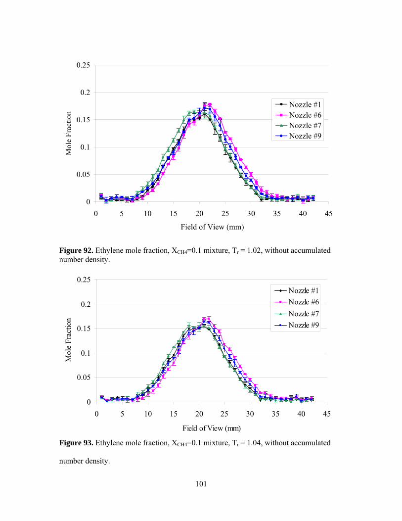
0
0.05
0.1
0.15
0.2
0.25
0 5 10 15 20 25 30 35 40 45
Field of View (mm)
Mol
e Fr
actio
n
Nozzle #1Nozzle #6Nozzle #7Nozzle #9
Figure 92. Ethylene mole fraction, XCH4=0.1 mixture, Tr = 1.02, without accumulated number density.
0
0.05
0.1
0.15
0.2
0.25
0 5 10 15 20 25 30 35 40 45
Field of View (mm)
Mol
e Fr
actio
n
Nozzle #1Nozzle #6Nozzle #7Nozzle #9
Figure 93. Ethylene mole fraction, XCH4=0.1 mixture, Tr = 1.04, without accumulated
number density.
101

0.14
0.15
0.16
0.17
0.18
0.19
0.2
0.21
0.22
0.23
0.99 1 1.01 1.02 1.03 1.04 1.05Tr
Mol
e Fr
actio
nNozzle #1Nozzle #6Nozzle #7Nozzle #9
Figure 94. Ethylene centerline mole fraction values for different nozzles.
10.65
11.15
11.65
12.15
12.65
13.15
13.65
14.15
0.99 1 1.01 1.02 1.03 1.04 1.05
Tr
Jet W
idth
(mm
)
Nozzle #1Nozzle #6Nozzle #7Nozzle #9
Figure 95. Ethylene jet widths for different nozzles.
102

Methane Mole Fractions for Different Nozzles.
Methane mole fraction profiles are presented for the next four figures, Figure 96
through Figure 99. The Gaussian curve fit of Tr = 1.04 case is also presented on each
figure to show the general pattern. The left side mole fraction value is higher than the
right side. That is caused by the calibration inaccuracy. As mentioned earlier, there is
difference associated with calibration data shown in Figure 64. Due to the small methane
concentration in the fuel compare to that of ethylene, the methane signal is easily
overwhelmed by even small signal noise.
In spite of low SNR, the profiles are consistent over different nozzles and
injection conditions. The mole fraction profile of condensed jet is distinctively above
from other cases which are also less desirable condition from the fuel mixing point of
view. As the injection temperature increases, the general pattern of mole fraction value
converges into one line as shown in Figure 99 except for Tr = 1.00. More importantly, the
mole fraction profile presented here for XCH4 = 0.1 mixture fuel has a different pattern
comparing to that of XCH4 = 0.2 mixture fuel. There is methane concentration at the jet
center of XCH4 = 0.2 mixture fuel. It is possible certain amount of methane molecules are
dispersing faster, and the rest of the methane molecules are remained at the jet center.
Furthermore, methane molecules are not condensed while ethylene molecules are
condensed. Because methane critical temperature is much lower than that of mixture fuel.
Thus it may not be in condensed phase letting methane disperses fast from the jet center.
Also, it is relatively light gas molecule comparing to ethylene that could spread out
quickly. And once it is dispersed to the jet edge, it is overwhelmed by turbulent flow for
mixing with nitrogen.
103

0
0.02
0.04
0.06
0.08
0.1
0 5 10 15 20 25 30 35 40 45
Field of View (mm)
Mol
e Fr
actio
nTr = 1.00Tr = 1.01Tr = 1.02Tr = 1.04Gaussian Fit
Figure 96. Methane mole fraction, XCH4 = 0.1 mixture, nozzle #1.
0
0.02
0.04
0.06
0.08
0.1
0 5 10 15 20 25 30 35 40 45
Field of View (mm)
Mol
e Fr
actio
n
Tr = 1.00Tr = 1.01Tr = 1.02Tr = 1.04Gaussian Fit
Figure 97. Methane mole fraction, XCH4 = 0.1 mixture, nozzle #6.
104

0
0.02
0.04
0.06
0.08
0.1
0 5 10 15 20 25 30 35 40 45
Field of View (mm)
Mol
e Fr
actio
nTr = 1.00Tr = 1.01Tr = 1.02Tr = 1.04Gaussian Fit
Figure 98. Methane mole fraction, XCH4 = 0.1 mixture, nozzle #7.
0
0.02
0.04
0.06
0.08
0.1
0 5 10 15 20 25 30 35 40 45
Field of View (mm)
Mol
e Fr
actio
n
Tr = 1.00Tr = 1.01Tr = 1.02Tr = 1.04Gaussian Fit
Figure 99. Methane mole fraction, XCH4 = 0.1 mixture, nozzle #9.
105

Nitrogen Mole Fractions for Different Nozzles.
Nitrogen mole fraction profiles are shown in Figure 100 through 103 as an ambient
gas representing the air in the combustor. The centerline deficit is well expected because
of the presence of the ethylene and methane molecules. These nitrogen mole fractions are
supporting the fact that the condensed jet is not well mixed with the nitrogen. Because,
the nitrogen mole fraction profile at the condensed jet has the lowest centerline value as
well as widest deficit width. This fact indicates the ambient nitrogen molecules are not
smeared to the condensed ethylene molecules. However, as the injection temperature
increases nitrogen mole fraction is proving better mixing with the fuel. The centerline
mole fraction is increased and the width is narrowed.
0.5
0.6
0.7
0.8
0.9
0 5 10 15 20 25 30 35 40 45
Field of View (mm)
Mol
e Fr
actio
n
Tr = 1Tr = 1.01Tr = 1.02Tr = 1.04
Figure 100. Nitrogen mole fraction, XCH4=0.1 mixture, nozzle #1.
106

0.5
0.6
0.7
0.8
0.9
0 5 10 15 20 25 30 35 40 45
Field of View (mm)
Mol
e Fr
actio
n
Tr = 1Tr = 1.01Tr = 1.02Tr = 1.04
Figure 101. Nitrogen mole fraction, XCH4=0.1 mixture, nozzle #6.
0.5
0.6
0.7
0.8
0.9
0 5 10 15 20 25 30 35 40 45
Field of View (mm)
Mol
e Fr
actio
n
Tr = 1Tr = 1.01Tr = 1.02Tr = 1.04
Figure 102. Nitrogen mole fraction, XCH4=0.1 mixture, nozzle #7.
107

0.5
0.6
0.7
0.8
0.9
0 5 10 15 20 25 30 35 40 45
Field of View (mm)
Mol
e Fr
actio
n
Tr = 1Tr = 1.01Tr = 1.02Tr = 1.04
Figure 103. Nitrogen mole fraction, XCH4=0.1 mixture, nozzle #9.
Mole Fraction Ratios of Ethylene to Methane for Different Nozzles.
Mole fraction ratio of ethylene to methane mole fraction is developed to
determine whether there is any preferential condensation within the supercritical jet. The
mole fraction ratios over the different nozzles are shown in Figure 104 through 107. The
centerline ratio value is generally higher than jet edge value. Also, much lareger errors
are involved at the jet center due to the small centerline mole fraction value of methane
signal. The centerline value is much higher than the fuel initial mixing ratio. If two
species are spreading out with the same rate, it should appear as a constant line at 9 the
same as the one shown in Figure 64. However, there might be different dispersion rate is
involved. The centerline value is much higher than initial mixing ratio and lower value at
the jet edge region. As mentioned previously, high noise associated with methane mole
fraction is primary reason for rising the centerline ratio value higher than it should be.
108

Every figure has large error bar at the jet center and unrealistic peak values which can be
considered abnormal value. So this might be one possible reason to rise up the ratio value
somewhat higher than where it should be, but generally high ratio value is observed as
can be seen in Figure 104 which has relatively low signal noise.
At the methane mole fraction section, it is observed methane molecules are
spreading out faster in the jet center. The differential dispersion rate between ethylene
and methane gas molecule can produce high ratio value at the jet center. Methane
molecules are spreading out faster than ethylene molecule at the jet center, this causes
higher mole fraction value than initial mixing ratio. Possibly, methane is not condensed
as much as ethylene. In other words, the condensation rate under the same temperature
condition is not equal to both gases. Light methane molecule in gaseous phase is
spreading out faster than heavy condensed ethylene molecules while both partially
condensed molecules are spreading out at the same rate. This is possible, because the
methane critical temperature is much lower than injection condition whereas the ethylene
critical temperature is the same as Tr = 1.02 case that is the condition that could produce
condensed ethylene jet, even if mixture gas exhibits different critical temperature point.
The ratio value at the jet edge is consistently lower than initial fuel mixing ratio.
The gaseous phase of methane molecules are spreading faster than the ethylene. The
number density of methane at the jet edge is larger than the number density in the fuel.
The methane molecule presence at the jet center is relatively small. This is rising high
mole fraction ratio at the jet center. Relatively large methane molecule as a result of
differential spreading out rate exists at the jet edge. This is lowering the mole fraction
109

ratio. Consequently, there is ethylene preferential condensation within the jet based on
the mole fraction ratios.
147
10131619222528
0 5 10 15 20 25 30 35 40 45
Field of View (mm)
Rat
io
Tr = 1.00Tr = 1.01Tr = 1.02Tr = 1.04Gaussian Fit
Figure 104. Mole fraction ratio, XCH4=0.1 mixture, nozzle #1.
147
10131619222528
0 5 10 15 20 25 30 35 40 45
Field of View (mm)
Rat
io
Tr = 1.00Tr = 1.01Tr = 1.02Tr = 1.04Gaussian Fit
Figure 105. Mole fraction ratio, XCH4=0.1 mixture, nozzle #6.
110
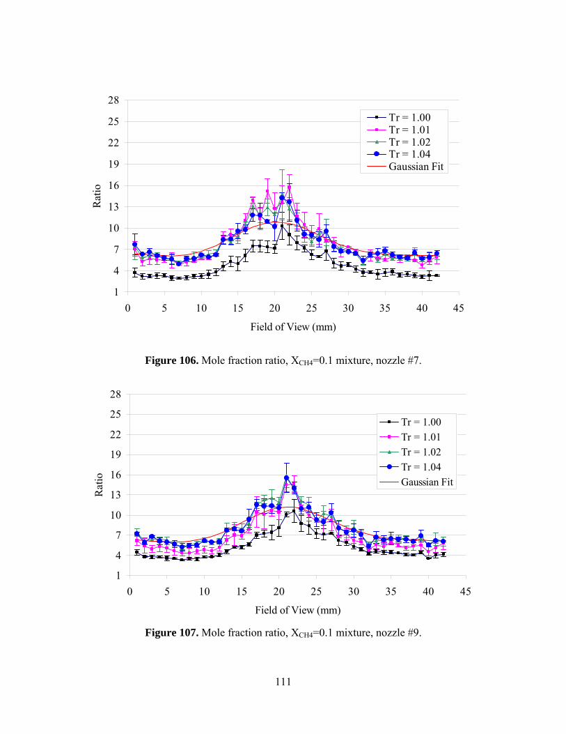
1
4
7
10
13
16
19
22
25
28
0 5 10 15 20 25 30 35 40 45
Field of View (mm)
Rat
io
Tr = 1.00Tr = 1.01Tr = 1.02Tr = 1.04Gaussian Fit
Figure 106. Mole fraction ratio, XCH4=0.1 mixture, nozzle #7.
1
4
7
10
13
16
19
22
25
28
0 5 10 15 20 25 30 35 40 45
Field of View (mm)
Rat
io
Tr = 1.00Tr = 1.01Tr = 1.02Tr = 1.04Gaussian Fit
Figure 107. Mole fraction ratio, XCH4=0.1 mixture, nozzle #9.
111

Jet Divergence Angle and Potential Core Length
The calculated potential core length is presented in the Figure 108 from the given
relations by Chehroudi et al. [10]. Generally, the potential liquid core decreases as the
injection temperature is increased, because the liquid jet produced at the lower injection
temperature has larger density. Therefore, the potential core length is longer than gaseous
jet which is increased injection temperature.
Also the jet divergence angle is calculated based on the relation given by
Dimotakis et al. [22]. This relationship is depends on bulk velocity and density ratio of
the sheer layer. See Appendix D for detailed relationship developed by him. The jet
divergence angle is shown in Figure 109. The condensed jet has relatively small
divergence angle and it is almost linearly increased as the injection temperature increases.
And based on this result, nozzle #9 has a little bit larger divergence angle but the
difference is not significantly large.
Consequently, the injection performance of nozzle 9 is spreading the fuel in a
redial direction and nozzle #1 is injecting the fuel in a axial direction. Because the nozzle
#9 has shortest potential core length while largest fuel divergence angle. In case of nozzle
#1 has longest potential core while narrowest divergence angle. Therefore, the nozzle #1
is suitable injector injecting the fuel to long supersonic flow combustor such as scramjet
engine.
112

17.4
17.6
17.8
18
18.2
18.4
18.6
18.8
0.99 1 1.01 1.02 1.03 1.04 1.05
Tr
z/d
Nozzle #1Nozzle #6Nozzle #7Nozzle #9
Figure 108. Potential core length for different injection temperature.
11.44
11.46
11.48
11.5
11.52
11.54
11.56
11.58
0.99 1 1.01 1.02 1.03 1.04 1.05Tr
Jet D
iver
genc
e A
ngle
Nozzle #1Nozzle #6Nozzle #7Nozzle #9
Figure 109. Jet divergence angle for different injection temperature, Units are in degrees.
113

V. Conclusions and Recommendations
Conclusions
Experiment Overview.
All tests are performed in a supercritical region injecting vertically into the
quiescent chamber simulating the environment of a Ramjet or scramjet combustor
section. Experimental research is conducted with four different research objectives of
determining species distribution profile in terms of mole fraction at the down-stream
location using Raman scattering technique.
This research starts with visualizing the global appearance of supercritical jet
using shadowgraph imaging technique to find the jet condensation condition. Then, the
Raman scattering technique is employed to identify species concentration profile at
down-stream location associated with the injection condition found by shadowgraph
technique.
Three different fuels are used for testing fluid along with four injection
temperature conditions with four injection nozzles.
Conclusions.
All the species concentration profile is determined over the different nozzles and
injection conditions. Each species mole fraction is determined based on the number
density. Ethylene mole fraction profile shows that the peak mole fraction value is located
at the jet centerline. Certain amounts of ethylene species are still concentrated at the jet
centerline at that location. Nitrogen has lowest value at the jet centerline which is
expected. The nitrogen deficit at the jet center is primarily due to the presence of ethylene
114

gas. Methane mole fraction also demonstrates that its peak value is maintained at the jet
centerline on XCH4 = 0.2 mixture case whereas evenly distributed methane mole fraction
is observed on XCH4 = 0.1 mixture case. Therefore, the first research objective
determining species distribution profile is accomplished.
The second research objective is determining whether the condensed jet effects on
the fuel mixing process or not. For this research objective, the test is conducted with four
different injection conditions from where a lot of condensed droplets are produced within
the jet to where the condensation is not significant elevating the injection temperature
from the each fuel’s critical temperature point. Centerline ethylene mole fraction of
condensed jet (Tr = 1.00) is higher than other injection cases which are less condensed
jets produce. As the injection temperature increases the centerline mole fraction value
decreases. Whereas, the nitrogen mole fraction profile shows that the centerline value
goes the other way as the injection temperature increases. In essence, the condensed jet
demonstrates relatively poor mixing behavior with the air. This phenomenon is the strong
evidence that the condensed jet is affecting on the fuel mixing rate and the condensed jet
is not preferable from fuel mixing perspective. In addition, the methane mole fraction has
the same trends to that of ethylene gas. The question of the second research objective has
been answered, therefore it is also accomplished.
The third research objectively is clarifying whether there is any preferential
condensation within the mixture jet or not. The mole fraction ratio of ethylene to methane
mole fraction of each mixture fuel is presented for this research objective. The methane
Raman signal is weak and has high SNR due to its small amount of presence in the fuel.
In spite of this reason, the mole fraction ratio of each fuel case consistently demonstrates
115

that there is preferential condensation within the jet. The methane which is light molecule
compare to ethylene is dispersing faster than ethylene (heavy molecule) at the jet center.
Both mixture cases, the methane mole fraction shows almost uniform dispersion which
means spreading out faster than the ethylene molecule does. This is because possibly the
amount of gaseous methane molecule is larger than that of ethylene molecules, since the
liquid phase ethylene jet is slowly spreading out at the jet center based on the answer of
previous objective. This differential spreading out rate forms relatively high mole fraction
ratio at the jet center and it becomes leveled at the outer edge of the jet by the turbulent
flow effects. In short, the methane molecules (light molecule) spread out faster than the
ethylene (heavy molecule) at the jet center. Therefore, the gas mole fraction ratio at the
downstream location does not have evenly distributed value in stead its centerline value
is higher than that of surrounds. The conclusion of third research objective is that there is
ethylene preferential condensation within jet.
The last research objective is to choose the nozzle performing better mixing
behavior with the air. Four nozzles are used and ethylene mole fraction profile is
compared at the same injection temperature ratio. The nozzle which has the smallest
centerline mole fraction value and the largest jet width is better nozzle than others.
Generally every four nozzle has almost the same performance in terms of centerline value
and jet width. It is hard to determine, but nozzle #1 which has no internal convergence
section and shortest final flow pass length is demonstrating better performance in terms
of centerline mole fraction value at each condition. Therefore, the nozzle #1 is
recommended for long combustion chamber.
116

Consequently, experimental results satisfy four research objectives. Furthermore,
this Raman study results will give enough information for comparing to the results of
Computer Fluid Dynamics (CFD) which will be studied in the near future.
Recommendations for Future Research
Since the thermo-dynamical property of the supercritical fuel is unique, there
might be a difference when it is injected into the air. This research is initially attempted
study to identify molecular distribution profile at z/d = 100 down-stream location
injecting the supercritical fuel into the quiescent chamber. It is difficult to draw
conclusion of the supercritical fuel species distribution profile with single observation
point. Therefore, the first recommendation for future research is to diversify the
observation point vertically along the jet line; near-field or potential core region,
transition region, and self-similar region. Thus the observation location might be z/d =
10, 40, 70, 100 to determine supercritical molecular species diffusion profile as it moves
away from nozzle exit plane.
The methane mole fraction of the fuel is small which is the primary reason
decreasing SNR and it degrades the accurate measurement of methane signal at that far
down-stream location. Increasing the methane mole fraction higher than 30% would be
recommended for the accurate measurement. In addition, increasing the chamber pressure
also recommended to the accurate measurement for the future research.
117

Appendix A: Injection Nozzle Design
Figure 110. Injection nozzle #6 base design, units are in inches.
118

Figure 111. Injection nozzle #1 and #6 designs.
119

Figure 112. Injection nozzle #7, #8, and #9 designs.
120

Appendix B: Least Square Method
The method of least square is used to find correlations to calibration of number
density of nitrogen and methane, ethylene. The purpose of the method of least square is
to minimize the sum of the squares of the fit’s offset (residual). If there is no
experimental error, the two sets of data point will form the line Y=C + DX. But, if there
is error, the line can be formed and it is necessary to find the best fitted line between the
two points. Consider seven different points, ( , )i ix y , i = 1..7.
1 1
2 2
7 7
C Dx yC Dx y
C Dx y
+ =+ =
+ =
There are two unknowns and seven equations. If there is an error, this set of
equation will not have a solution. Rewriting this equation set in a matrix form,
1 1
2 2
3 3
4 4
5 5
6 6
77
111
, or1111
x yx yx y
Cx y AX b
Dx yx y
yx
⎛ ⎞ ⎛ ⎞⎜ ⎟ ⎜ ⎟⎜ ⎟ ⎜ ⎟⎜ ⎟ ⎜ ⎟⎜ ⎟ ⎜ ⎟⎛ ⎞
= =⎜ ⎟⎜ ⎟ ⎜ ⎟⎝ ⎠⎜ ⎟ ⎜ ⎟
⎜ ⎟ ⎜ ⎟⎜ ⎟ ⎜ ⎟⎜ ⎟ ⎜ ⎟
⎝ ⎠⎝ ⎠
It can’t be solved because the points are not on a line. Therefore they are solved by
least squares:
1, ( )T T TA A X A b or X A A A b∧ ∧
−= = T
In this study, variable, ix , (i = 1..7) are the species number density determined by
the perfect gas law. b is the corresponding signal intensities.
121

Appendix C: Supercritical Fuel Injection System and Operating Procedure
Figure 113. Schematic of supercritical injection flow.
122

Figure 114. Supercritical injection jet control program.
123

124

125

126

127

128

Appendix D: Jet Divergence Angle Equation
Jet divergence angles of different nozzles calculated using the relationship
presented by Dimotakis et al. [22]. This relationship is based on bulk velocity and density
ratio of the shear layer.
( )( )
1/ 2
1/ 200
1/ 20 0
00 0
110.17 1
1 /1 2.91 1 /
uu
u uuu uu
ρρρδ
ρρρ
∞∞
∞
∞∞ ∞
∞
⎧ ⎫⎧ ⎡ ⎤⎛ ⎞⎛ ⎞⎪ ⎪⎪ ⎢ ⎥− ⎜ ⎟−⎜ ⎟⎪ ⎪⎪ ⎢ ⎥⎝ ⎠⎛ ⎞⎪ ⎪⎪⎝ ⎠ ⎣ ⎦= + −⎨ ⎬⎨ ⎜ ⎟⎡ ⎤ ⎡ +⎝ ⎠⎛ ⎞ ⎛ ⎞⎪ ⎪⎪ +⎢ ⎥ ⎢+ ⎜ ⎟ ⎜ ⎟⎪ ⎪⎪ −
⎫⎪⎪⎪⎬⎤ ⎪⎥ ⎪⎣ ⎦⎢ ⎥⎝ ⎠ ⎝ ⎠⎪ ⎪⎪⎣ ⎦⎩ ⎭⎩ ⎪⎭
(20)
For this study, a supercritical jet is injected into a quiescent chamber, the velocity
ratio is zero, simplifying the following equation.
1/ 2
0
0.17 1 ρδρ∞
⎡ ⎤⎛ ⎞⎢ ⎥= − ⎜ ⎟⎢ ⎥⎝ ⎠⎣ ⎦
(21)
129

Appendix E: Ethylene Vibrational Mode
There are six different kinds of vibrational modes for every molecules [23].
Generally, it has stretching and bending vibrations. Stretching vibration has symmetric
and asymmectric vibrations. Bending vibaration has in-plane and out of plane vibrations.
In-plane vibration has rocking and scissoring vibrations while out of plane has wagging
and twisting vibrations [23].
21 3
54 6
98
7
12
1110
Figure 115. Ethylene molecule’s vibrational modes [23].
Ethylene molecule has twelve different types of vibration as shown in Figure 108.
1 is a CH2 symmetric stretching, 2 is a CC stretching, and 3 is a CH2 scissoring. 4 is a
CH2 twisting, 5 is a asymmetric CH2 stretching, and 6 is a CH2 rocking. 7 and 8 are
CH2 wagging, 9 is a CH2 asymmetric stretching, and 10 is a CH2 rocking. 11 is CH2
symmetric stretching, 12 is a CH2 scissoring mode. Each vibrational mode has specific
frequencies that can be detected by molecular spectroscopy. Table 6 is showing the
130

specific Raman frequencies corresponding to the ethylene vibrational modes [24]. Other
vibrational mode is not the Raman active. According to Table 6, ethylene I is a
vibrational mode 3 (v3), ethylene II is a vibrational mode 2 (v2), and ethylene III is a
vibrational mode 1 (v1).
Table 6. Raman shift for ethylene molecule’s vibrational mode [24].
Mode Type of mode Raman frequency (cm-1) Phase
1 CH2 symmetric stretching 3026.4 Gas 2 CC stretching 1622.6 Gas 3 CH2 scissoring 1342.2 Gas 5 CH2 asymmetric stretching 3102.5 Gas 6 CH2 rocking 1236 Liquid 8 CH2 wagging 943 Liquid
131

References
1. Edwards, T., “USAF Supercritical Hydrocarbon Fuels Interests”, AIAA paper 93-
0807, January 1993 2. Maurice, L., Edwards, T., and Griffiths, J. “Liquid Hydrocarbon Fuels for Hypersonic
Combustion”. Progress in Astronautics and Aeronautics V189: Scramjet Propulsion, Ed. E.T. Curran and S.N.B. Murthy. American Institute of Aeronautics and Astronautics, Inc. VA, 2000, pp 757-822.
3. Edwards, T., Anderson, S. D., “Results of High Temperature JP-7 Cracking Asscssment,”
AIAA Paper 93-0806, AIAA Aerospace Sciences Meeting, Reno, NV, Jan. 1993. 4. Lin, K.-C., Cox-Stouffer, S. K., Kennedy, P.J., and Jackson, T. A., “expansion of
Supercritical Methane/Ethylene Jets in a Quiescent Subcritical Environment” AIAA paper 03-0483, January 2003.
5. Wu, P.-k., Shahnam, M., Kirkendall, K. A., Carter, C. D., and Nejad, A. S.,
“Expansion and Mixing Processes of Underexpanded Supercritical Fuel Jets Injected into Superheated Conditions”, Journal of Propulsion and Power, Vol. 15, No. 5, pp.642-649, 1999.
6. http://www.pnl.gov/supercriticalfluid/about.stm 7. Huber, M. L., NIST Standard Reference Database 4: NIST Thermophysical Properties
of Hydrocarbon Mixtures Database (SUPERTRAPP), Version 4, 1999. 8. Lin, K.-C., Cox-Stouffer, S. K., and Jackson, T. A., “Structures and Phase Transition
Processes of Supercritical Methane/Ethylene Mixtures Injected into a Subcritical Environment” Combustion and Science Technology, 178: pp 129-160, 2006.
9. Crist, S., Sherman, P. M., and Glass, D. R., “Study of the highly underexpanded sonic
jet”, AIAA Journal, 4, 68. 1968. 10. Branam, R., and Mayer, W., “Characterization of Cryogenic Injection at Supercritical
Pressure,” Journal of Propulsion and power, Vol. 19, No. 3, pp. 342-355, May/Jun 2003
11. Chehroudi, B., Talley, D., and Coy, E., “Initial Growth Rate and Visual
Characteristics of a Round Jet into a Sub- to Supercritical Environment of Relevance to Rocket, Gas Turbine, and Diesel Engines,” AIAA paper number 99-0206, 37th AIAA Aerospace Sciences Meeting and Exhibit, Reno, NV, pp. 6-7, 1999.
132

12. Schetz, J. A., “Injection and Mixing in Turbulent Flow”, Progress in Aeronautics and Astronautics, Vol 68, AIAA 1980, pp. 19-84. 13. Ewen, smith., and Geoffrey, Dent., Modern Raman Spectroscopy: A Practical
Approach. Southern Gate : John Wiley and sons Ltd. England. 2005. 14. Schrader, B., Infrared and Raman Spectroscopy; Chapter 4. New York : VCH
Publishers Inc. 1995. 15. Eckbreth, Alan C., Laser Diagnostics for Combustion Temperature and Species.
Cambridge: Abacus. 1995. 16. Ferraro, J.R., and Kazuo, N. Introductory Raman Spectroscopy. San Diego:
Academic Press. 1994. 17. McCreery, R. L., Raman Spectroscopy for Chemical Analysis. John Wiley & Sons,
Inc. 2000. 18. Holman, J. P., Experimental Methods for Engineers. McGrow-Hill, Co. 2001. 19. Yang, Wen-Jei. Handbook of Flow Visualization. Taylor and Francis. 1989. 20. www.geocities.com 21. http://webbook.nist.gov 22. Dimotakis, P.E., “Two-dimensional Shear-layer Entrainment,” AIAA Journal, vol.
24, no. 11, pp. 1791-1796, 1986. 23. www.shodor.org/succeed/compchem/labs/vibrations/ 24. www.webbook.nist.gov/cgi/cbook/
133

Vita
Captain Young Man An, Republic of Korea Army, graduated from Korea
Military Academy where he graduated with a Bachelor of Science degree in Physics in
March 2000. He was commissioned as a 2nd lieutenant and assigned to 28th infantry
division as a platoon leader. He served as an aid-de-camp of a division commander for
one year. He entered Infantry Officer’s Advanced Course for six months where he could
broaden and enrich the knowledge on military operations and command philosophy.
Upon graduation he was selected to the Graduate School of Engineering and
management, Air Force Institute of Technology.
Upon achievement of a masters of science in Aeronautical Engineering, Capt. An
will continue on to conduct his military career assuming company commander of 11th
Mechanized Infantry Division in the First ROK field army, South Korea.
134

135
REPORT DOCUMENTATION PAGE Form Approved OMB No. 074-0188
The public reporting burden for this collection of information is estimated to average 1 hour per response, including the time for reviewing instructions, searching existing data sources, gathering and maintaining the data needed, and completing and reviewing the collection of information. Send comments regarding this burden estimate or any other aspect of the collection of information, including suggestions for reducing this burden to Department of Defense, Washington Headquarters Services, Directorate for Information Operations and Reports (0704-0188), 1215 Jefferson Davis Highway, Suite 1204, Arlington, VA 22202-4302. Respondents should be aware that notwithstanding any other provision of law, no person shall be subject to an penalty for failing to comply with a collection of information if it does not display a currently valid OMB control number. PLEASE DO NOT RETURN YOUR FORM TO THE ABOVE ADDRESS. 1. REPORT DATE (DD-MM-YYYY)
13-09-2007 2. REPORT TYPE
Master’s Thesis 3. DATES COVERED (From – To)
August 2005 – September 2007
5a. CONTRACT NUMBER
5b. GRANT NUMBER
4. TITLE AND SUBTITLE RAMAN SCATTERING STUDY OF SUPERCRITICAL
BI-COMPONENT MIXTURES INJECTED INTO A SUBCRITICAL ENVIRONMENT
5c. PROGRAM ELEMENT NUMBER
5d. PROJECT NUMBER 5e. TASK NUMBER
6. AUTHOR(S) An, Young Man., Captain, ROKA
5f. WORK UNIT NUMBER
7. PERFORMING ORGANIZATION NAMES(S) AND ADDRESS(S) Air Force Institute of Technology Graduate School of Engineering and Management (AFIT/EN) 2950 Hobson Way, Building 640 WPAFB OH 45433-8865
8. PERFORMING ORGANIZATION REPORT NUMBER
AFIT/GA/ENY/07-S01 10. SPONSOR/MONITOR’S ACRONYM(S)
AFRL/PRAS
9. SPONSORING/MONITORING AGENCY NAME(S) AND ADDRESS(ES) AFRL Propulsion Directorate 1950 5th street WPAFB OH 45433-7251
11. SPONSOR/MONITOR’S REPORT NUMBER(S)
12. DISTRIBUTION/AVAILABILITY STATEMENT APPROVED FOR PUBLIC RELEASE; DISTRIBUTION UNLIMITED.
13. SUPPLEMENTARY NOTES 14. ABSTRACT This research studies the species distribution profiles of methane/ethylene bi-components at downstream locations filled with subcritical nitrogen in a closed chamber. Unique thermodynamic and transport properties of supercritical fluids along with phase transition phenomena during fuel injection process can significantly change combustion characteristics inside a scramjet combustor. Plume properties of supercritical jets are of great interests to the studies of fuel/air mixing and subsequent combustion. The primary goal of this research is to help to clarify whether there is any preferential condensation within the condensed jets. The Raman Scattering technique is used to quantify spatial distribution of injected methane and ethylene. Each species distribution profile is developed in terms of mole fraction. Results demonstrated there is ethylene preferential condensation within the supercritical bi-component mixture of the jet. It also showed the condensation phenomenon is less desirable for combustion. 15. SUBJECT TERMS Ethylene/methane mixture fuel, Supercritical injection jet, Raman scattering, Condensation, Mole fraction profile
16. SECURITY CLASSIFICATION OF:
19a. NAME OF RESPONSIBLE PERSON Dr. Paul I. King
a. REPORT
U
b. ABSTRACT
U
c. THIS PAGE
U
17. LIMITATION OF ABSTRACT
UU
18. NUMBER OF PAGES
154
19b. TELEPHONE NUMBER (Include area code) (937) 255-3636, ext 4628 ([email protected])
Standard Form 298 (Rev. 8-98) Prescribed by ANSI Std. Z39-18