air force institute of technology - dtic · talkies. together these devices operate across a wide...

Passive Geolocation of Low-Power Emitters

in Urban Environments Using TDOA

THESIS

Myrna B. Montminy, Captain, USAF

AFIT/GE/ENG/07-16

DEPARTMENT OF THE AIR FORCEAIR UNIVERSITY

AIR FORCE INSTITUTE OF TECHNOLOGY

Wright-Patterson Air Force Base, Ohio

APPROVED FOR PUBLIC RELEASE; DISTRIBUTION UNLIMITED.

The views expressed in this thesis are those of the author and do not reflect theofficial policy or position of the United States Air Force, Department of Defense, orthe United States Government.

AFIT/GE/ENG/07-16



THESIS

Presented to the Faculty

Department of Electrical and Computer Engineering

Graduate School of Engineering and Management

Air Force Institute of Technology

Air University

Air Education and Training Command

In Partial Fulfillment of the Requirements for the

Degree of Master of Science in Electrical Engineering

Myrna B. Montminy, B.S.E.E.

Captain, USAF

March 2007

APPROVED FOR PUBLIC RELEASE; DISTRIBUTION UNLIMITED.

AFIT/GE/ENG/07-16

Abstract

Low-power devices such as key fobs, cell phones, and wireless routers are com-

monly used to control Improvised Explosive Devices (IEDs) and as communications

nodes for command and control. Quickly locating the source of these signals is dif-

ficult, especially in an urban environment where buildings and towers can cause in-

terference. This research presents a geolocation system that combines the attributes

of several proven geolocation and error mitigation methods to locate an emitter of

interest in an urban environment. The proposed geolocation system uses a Time

Difference of Arrival (TDOA) technique to estimate the location of the emitter of

interest. Using multiple sensors at known locations, TDOA estimates are obtained

by cross-correlating the signal received at all the sensors. A Weighted Least Squares

(WLS) solution is used to estimate the emitter’s location. If the variance of this lo-

cation estimate is too high, a sensor is detected and identified as having a Non-Line

of Sight (NLOS) path from the emitter. This poorly located sensor is then removed

from the geolocation system and a new position estimate is calculated with the re-

maining sensor TDOA information. The performance of the TDOA system is assessed

through modeling and simulations. Test results confirm the feasibility of identifying

a NLOS sensor, thereby improving the geolocation system’s accuracy in an urban

environment.

iv

Acknowledgements

I would like to thank my husband. Your support and understanding got me

through many hard and long days. Thank you for your love and encouragement.

Myrna B. Montminy

v

Table of ContentsPage

Abstract . . . . . . . . . . . . . . . . . . . . . . . . . . . . . . . . . . . . . iv

Acknowledgements . . . . . . . . . . . . . . . . . . . . . . . . . . . . . . . v

List of Figures . . . . . . . . . . . . . . . . . . . . . . . . . . . . . . . . . ix

List of Tables . . . . . . . . . . . . . . . . . . . . . . . . . . . . . . . . . . xi

I. Introduction . . . . . . . . . . . . . . . . . . . . . . . . . . . . . 11.1 Background . . . . . . . . . . . . . . . . . . . . . . . . . 1

1.2 Problem Statement . . . . . . . . . . . . . . . . . . . . . 21.3 Current Research . . . . . . . . . . . . . . . . . . . . . . 21.4 Scope and Application . . . . . . . . . . . . . . . . . . . 2

1.5 Assumptions . . . . . . . . . . . . . . . . . . . . . . . . 3

1.6 Research Benefits . . . . . . . . . . . . . . . . . . . . . . 31.7 Standards . . . . . . . . . . . . . . . . . . . . . . . . . . 41.8 Approach / Methodology . . . . . . . . . . . . . . . . . 4

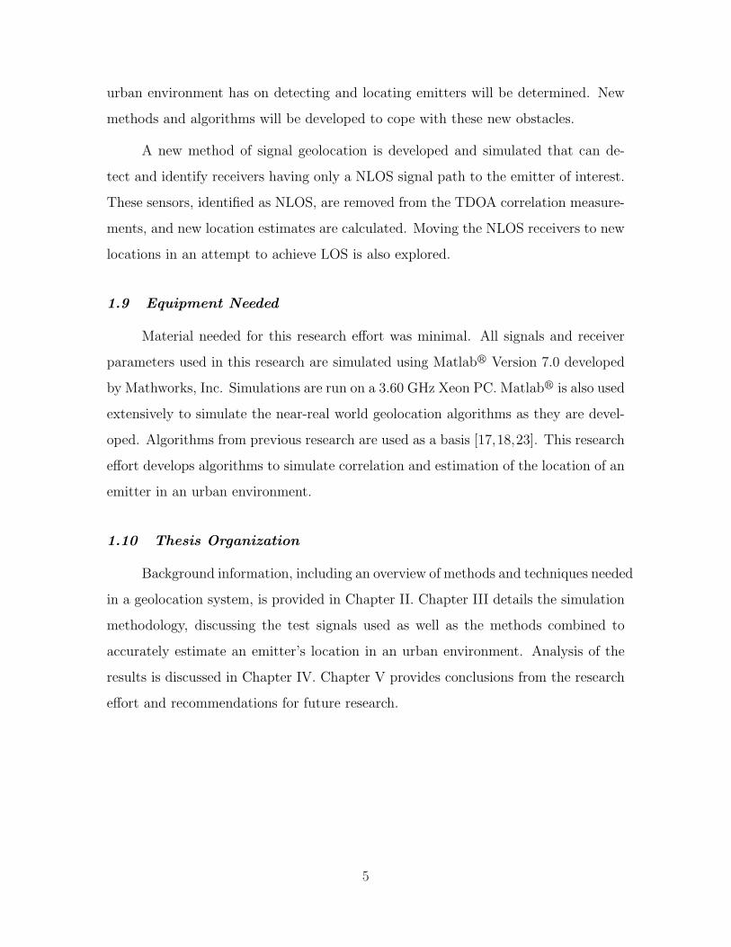
1.9 Equipment Needed . . . . . . . . . . . . . . . . . . . . . 5

1.10 Thesis Organization . . . . . . . . . . . . . . . . . . . . 5

II. Background . . . . . . . . . . . . . . . . . . . . . . . . . . . . . . 6

2.1 Overview . . . . . . . . . . . . . . . . . . . . . . . . . . 62.2 Methods for Locating Emitters . . . . . . . . . . . . . . 6

2.2.1 Angle of Arrival (AOA) . . . . . . . . . . . . . 6

2.2.2 Frequency Difference of Arrival (FDOA) . . . . 7

2.2.3 Time of Arrival (TOA) . . . . . . . . . . . . . . 8

2.2.4 Time Difference of Arrival (TDOA) . . . . . . . 9

2.3 Time Difference of Arrival Estimation (TDOA) . . . . . 11

2.3.1 Cross Correlation Function . . . . . . . . . . . . 122.3.2 Correlation Window Size . . . . . . . . . . . . . 132.3.3 Ambiguity Function . . . . . . . . . . . . . . . . 14

2.4 Estimation of Low-Power Emitter Location . . . . . . . 152.4.1 Taylor Series Approximation . . . . . . . . . . . 17

2.4.2 Closed-Form Solution . . . . . . . . . . . . . . . 172.4.3 Hyperbolic Asymptotes . . . . . . . . . . . . . . 17

2.5 Over-Approximation . . . . . . . . . . . . . . . . . . . . 18

2.5.1 Divide and Conquer Position Estimation Method 19

vi

5.2 Linear Weighted Least Squares (WLS) Algorithm 19

2.6 Urban Environment Characteristics . . . . . . . . . . . . 212.6.1 Multipath . . . . . . . . . . . . . . . . . . . . . 21

2.6.2 Non-Line of Sight (NLOS) . . . . . . . . . . . . 22

2.7 Receiver Error Identification and Mitigation . . . . . . . 23

2.7.1 Time-History Based Approach . . . . . . . . . . 24

2.7.2 Residual Ranking . . . . . . . . . . . . . . . . . 24

2.7.3 Receiver Geometrical Layout . . . . . . . . . . . 25

2.8 Summary . . . . . . . . . . . . . . . . . . . . . . . . . . 27

III. Simulation Methodology . . . . . . . . . . . . . . . . . . . . . . . 29

3.1 Overview . . . . . . . . . . . . . . . . . . . . . . . . . . 293.2 Geolocation System . . . . . . . . . . . . . . . . . . . . 29

3.3 Sensor Parameters . . . . . . . . . . . . . . . . . . . . . 303.4 Cross-Correlation . . . . . . . . . . . . . . . . . . . . . . 31

3.4.1 Correlation Technique . . . . . . . . . . . . . . 31

3.4.2 Correlation Window . . . . . . . . . . . . . . . 323.4.3 Sampling Frequency . . . . . . . . . . . . . . . 33

3.4.4 Smoothing Function . . . . . . . . . . . . . . . 34

3.4.5 Resolution . . . . . . . . . . . . . . . . . . . . . 343.5 Position Estimation Using WLS Estimator . . . . . . . . 36

3.6 Detection and Identification of NLOS Receiver(s) . . . . 40

3.6.1 Approach . . . . . . . . . . . . . . . . . . . . . 41

3.6.2 Sensor Error Mitigation . . . . . . . . . . . . . 42

3.6.3 Emitter Position Variance . . . . . . . . . . . . 433.6.4 Recommended Sensor Locations . . . . . . . . . 47

3.7 Emitter Signal Generation . . . . . . . . . . . . . . . . . 48

3.7.1 Baseline Signal: BPSK Waveform Signal . . . . 48

3.7.2 Test Signal: GMSK Waveform Signal . . . . . . 49

3.7.3 Noise Generation . . . . . . . . . . . . . . . . . 513.8 Urban Environment Generation . . . . . . . . . . . . . . 523.9 Summary . . . . . . . . . . . . . . . . . . . . . . . . . . 52

IV. Geolocation Results and Analysis . . . . . . . . . . . . . . . . . . 53

4.1 Overview . . . . . . . . . . . . . . . . . . . . . . . . . . 534.2 System Results and Analysis: Baseline BPSK Signal . . 53

4.2.1 BPSK Signal Precision Characteristics . . . . . 53

4.2.2 Scenario A: Effects of Data Rate on Position Es-timate . . . . . . . . . . . . . . . . . . . . . . . 55

4.2.3 Scenario B: Effects of Correlation Window on Po-sition Estimate . . . . . . . . . . . . . . . . . . 56

vii

2.4 Scenario C: Favorable Sensor Configuration . . . 57

4.2.5 Scenario D: NLOS Sensor Configuration . . . . 58

4.2.6 Scenario E: Poorly Located LOS Sensor Configu-rations . . . . . . . . . . . . . . . . . . . . . . . 61

4.3 Other Signal Results . . . . . . . . . . . . . . . . . . . . 67

4.4 Summary . . . . . . . . . . . . . . . . . . . . . . . . . . 67

V. Conclusions and Future Work Recommendations . . . . . . . . . 695.1 Summary . . . . . . . . . . . . . . . . . . . . . . . . . . 69

5.2 Conclusions . . . . . . . . . . . . . . . . . . . . . . . . . 695.3 Recommendations for Future Work . . . . . . . . . . . . 70

Appendix A. Matlab Code . . . . . . . . . . . . . . . . . . . . . . . . 71

List of Abbreviations . . . . . . . . . . . . . . . . . . . . . . . . . . . . . . 100

Bibliography . . . . . . . . . . . . . . . . . . . . . . . . . . . . . . . . . . 101

viii

List of FiguresFigure Page

2.1. Triangulation. . . . . . . . . . . . . . . . . . . . . . . . . . . . 7

2.2. FDOA contours. . . . . . . . . . . . . . . . . . . . . . . . . . . 8

2.3. TDOA hyperbolic curves. . . . . . . . . . . . . . . . . . . . . . 10

2.4. Example configuration of two receivers and one emitter. . . . . 11

2.5. Correlation of two received signals. . . . . . . . . . . . . . . . . 12

2.6. Cross correlation example. . . . . . . . . . . . . . . . . . . . . 13

2.7. Auto-correlation of GSM signal. . . . . . . . . . . . . . . . . . 14

2.8. Complex ambiguity function. . . . . . . . . . . . . . . . . . . . 16

2.9. Geolocation using TDOA hyperbolas. . . . . . . . . . . . . . . 18

2.10. Geolocation using hyperbolic asymptotes. . . . . . . . . . . . . 19

2.11. Urban environment and multipath. . . . . . . . . . . . . . . . . 21

2.12. Multipath signals. . . . . . . . . . . . . . . . . . . . . . . . . . 22

2.13. NLOS signal path. . . . . . . . . . . . . . . . . . . . . . . . . . 23

2.14. NLOS effect on TDOA location estimate. . . . . . . . . . . . . 23

2.15. BS layout. . . . . . . . . . . . . . . . . . . . . . . . . . . . . . 26

2.16. Good geometry. . . . . . . . . . . . . . . . . . . . . . . . . . . 27

3.1. Example sensor configuration with emitter. . . . . . . . . . . . 29

3.2. Passive geolocation system. . . . . . . . . . . . . . . . . . . . . 30

3.3. Estimated TDOA hyperbolas. . . . . . . . . . . . . . . . . . . . 32

3.4. Correlation windows and their autocorrelations. . . . . . . . . . 33

3.5. Sampling rates compared. . . . . . . . . . . . . . . . . . . . . . 34

3.6. Smoothing function. . . . . . . . . . . . . . . . . . . . . . . . . 35

3.7. Geometry of emitter and N sensors. . . . . . . . . . . . . . . . 37

3.8. Estimated position using Torrieri’s method. . . . . . . . . . . . 40

3.9. NLOS sensor detection and identification. . . . . . . . . . . . . 41

ix

Figure Page

3.10. NLOS sensor configuration with intermediate position estimates. 44

3.11. Sensor position estimate residuals. . . . . . . . . . . . . . . . . 46

3.12. GSM frame details. . . . . . . . . . . . . . . . . . . . . . . . . 50

3.13. GSM signal pulses. . . . . . . . . . . . . . . . . . . . . . . . . . 50

3.14. Cross-correlation of GSM signal pulses. . . . . . . . . . . . . . 51

3.15. Simulated reflector and its effects. . . . . . . . . . . . . . . . . 52

4.1. BPSK signal and its autocorrelation. . . . . . . . . . . . . . . . 54

4.2. Favorable LOS configuration. . . . . . . . . . . . . . . . . . . . 55

4.3. Data rate comparison results. . . . . . . . . . . . . . . . . . . . 56

4.4. Correlation window comparison results. . . . . . . . . . . . . . 57

4.5. Favorable LOS configuration data. . . . . . . . . . . . . . . . . 58

4.6. NLOS configurations. . . . . . . . . . . . . . . . . . . . . . . . 59

4.7. NLOS configuration data. . . . . . . . . . . . . . . . . . . . . . 59

4.8. Variance and position error with NLOS sensor removed. . . . . 61

4.9. Poor LOS sensor configurations. . . . . . . . . . . . . . . . . . 62

4.10. Poor LOS configuration data. . . . . . . . . . . . . . . . . . . . 63

4.11. Poor zig-zag LOS sensor configuration. . . . . . . . . . . . . . . 64

4.12. Poor zig-zag LOS (5 sensor) configuration data. . . . . . . . . . 65

4.13. Poorly located LOS sensor removed. . . . . . . . . . . . . . . . 66

4.14. Variance and position error with NLOS sensor removed. . . . . 66

4.15. Autocorrelations of BPSK and GSM signals. . . . . . . . . . . 67

x

List of TablesTable Page

3.1. Signal sampling parameters. . . . . . . . . . . . . . . . . . . . . 36

xi



I. Introduction

1.1 Background

Low-power emitters are greatly contributing to the complexity of the electronic

warfare problem. They are commonly used to control IEDs, often detonating the

IEDs remotely with no warning to those who are targeted. Various emitters can also

be used by terrorists for command and control devices. Quickly locating the source of

the detonation signal is difficult, especially in an urban environment where buildings

and other signals can cause interference. This research presents a geolocation system

that use time difference of arrival (TDOA) to locate emitters of interest in an urban

environment.

Signals of interest, including signals from airplanes and radars, are detected

with receivers located and controlled by operators at a safe distance. Now, emitters

of interest include key fobs, cordless phones, cell phones, wireless routers, and walkie-

talkies. Together these devices operate across a wide range of the radio frequency

spectrum. The diversity of these emitters presents a significant force protection chal-

lenge because little is currently known about how to locate them.

The urban environment introduces additional challenges, including multipath,

signal scattering, and widespread interfering signals. These complications make it dif-

ficult and sometimes impossible to detect emitters, especially from the safe stand-off

distance that most geolocation systems currently use. New systems must have the

ability to approach much closer to the emitter to detect its signal, while keeping the

military controller safe from harm. This requirement means its possible deployment

onto an unmanned aerial vehicle (UAV) or unmanned ground vehicle (UGV). De-

ploying the geolocation system onto a UAV adds size and weight restrictions to the

1

already complex problem. These challenges highlight some of the many aspects that

this difficult problem presents.

1.2 Problem Statement

The purpose of this research is to provide a background on geolocation methods

and recommend methods that can be used to locate emitters within an urban envi-

ronment through modeling and simulation. This capability can lead to alternative

approaches to exploit the enemy, not only by locating possible IED detonators, but

also locating cell phones and communications nodes that may be used by the enemy

for command and control purposes.

1.3 Current Research

When a signal arrives at two moving, spatially separated receivers, the receivers

measure a difference in phase and frequency. The time that a signal arrived at two

spatially separate receivers also yields helpful information. These characteristics are

the basis for four methods of geolocation: 1) the angle of arrival (AOA) method that

locates a position using the directional angle of a signal, 2) the frequency difference

of arrival (FDOA) that determines the position of the emitter from the difference in

frequency of the signal measured between two receivers, 3) the time of arrival (TOA)

technique that calculates the position of the emitter using the precise time the signal

arrives at multiple receivers, and 4) time difference of arrival (TDOA) which uses the

difference in time a signal is received at two or more receivers to determine the location

of an emitter. In passively locating emitters, the TDOA and FDOA approaches offer

several advantages over both the AOA and TOA methods. Current research of each

of these emitter location techniques is discussed in more detail in Chapter II.

1.4 Scope and Application

This research investigates a process for locating low-power devices. As men-

tioned earlier, the emitters of interest are found in a wide variety of applications

2

ranging from remote controlled toys, to household electronics, to wireless communi-

cations. The research presented provides background on several current geolocation

methods and modify and apply them to locate emitters in the presence of multipath

and noise that are abundant in urban environments.

1.5 Assumptions

Specific limits and assumptions are imposed to make the problem solvable within

time and equipment availability constraints. It is assumed that the emitter of interest

is stationary and within detection range of several sensors. While the emitter location

is unknown, the emitter’s signal structure, including general waveform and bandwidth,

can be recognized. Approximation methods for estimating a single solution from

a set of multiple solutions are chosen from those readily available to the technical

community, including the estimation work of Knapp and Torrieri [15, 28]. These

methods are explained in more detail in Chapter II. It is also assumed that there are

no other signals in the area that may cause interference or overlap with the low-power

emitter’s signal being located.

1.6 Research Benefits

Results from this research are anticipated to have several applications. First,

the results will lead the U.S. military one step closer to having the ability to passively

locate unknown emitters. For this research, passive geolocation is defined as the ability

to geolocate an emitter by processing its radio frequency (RF) emissions. This allows

the emitter to be geolocated without being interrogated. Passive capability is crucial

in locating emitters that may be used for IED detonation, hostile jamming, or as

communications nodes because it can be accomplished without alerting the enemy. It

may also benefit search and rescue missions and law enforcement surveillance. Second,

the algorithms and geolocation methods that are developed as a part of this research

can be applied to current systems or added later to mobile receiver systems. Finally,

3

a complete geolocation system will be proposed that incorporates several different

research efforts in this area.

1.7 Standards

For this research to be successful, the location of an emitter must be accurate to

within ten meters. This accuracy is important in urban environments because other

emitters may be near the emitter of interest. If the error is greater than ten meters,

other emitters within the error range may be mistaken for the emitter of interest. Ten

meters is a reasonable distance because it can narrow down the location of the emitter

of interest to a specific building, park, or section of street. Accurate geolocation is

essential in the military’s ability to weaken the enemy and protect its troops.

1.8 Approach / Methodology

This research begins by investigating current methods of locating signals to

determine the best approach to locate an unknown emitter. This preliminary inves-

tigation and its results can be found in Chapter II. After deciding on a geolocation

approach, factors that may impede the goals of this research are considered. These

factors include emitter signal strength, tolerable noise level, and estimation schemes.

As these factors become more defined, more assumptions may be needed.

The research then focuses on the main problem: locating an unknown emitter in

an urban environment. As mentioned previously, the urban environment introduces

many obstacles that make it difficult to detect and locate signal sources. Buildings

can reflect signals, allowing multiple copies of the same signal to arrive at a receiver

at different times and signal strengths, also known as multipath. Many other emitters

can produce signals spanning a wide range of the frequency spectrum. These added

signals can cause interference and may be strong enough to hide the emitter that

needs to be located. The TDOA method of signal geolocation has been widely used

to locate signal sources. This research combines the TDOA geolocation method with

error detection techniques to effectively locate an emitter of interest. The impact the

4

urban environment has on detecting and locating emitters will be determined. New

methods and algorithms will be developed to cope with these new obstacles.

A new method of signal geolocation is developed and simulated that can de-

tect and identify receivers having only a NLOS signal path to the emitter of interest.

These sensors, identified as NLOS, are removed from the TDOA correlation measure-

ments, and new location estimates are calculated. Moving the NLOS receivers to new

locations in an attempt to achieve LOS is also explored.

1.9 Equipment Needed

Material needed for this research effort was minimal. All signals and receiver

parameters used in this research are simulated using Matlabr Version 7.0 developed

by Mathworks, Inc. Simulations are run on a 3.60 GHz Xeon PC. Matlabr is also used

extensively to simulate the near-real world geolocation algorithms as they are devel-

oped. Algorithms from previous research are used as a basis [17,18,23]. This research

effort develops algorithms to simulate correlation and estimation of the location of an

emitter in an urban environment.

1.10 Thesis Organization

Background information, including an overview of methods and techniques needed

in a geolocation system, is provided in Chapter II. Chapter III details the simulation

methodology, discussing the test signals used as well as the methods combined to

accurately estimate an emitter’s location in an urban environment. Analysis of the

results is discussed in Chapter IV. Chapter V provides conclusions from the research

effort and recommendations for future research.

5

II. Background

2.1 Overview

This chapter reviews literature of several geolocation methods and estimation

techniques that may be used to passively locate low-power emitters while identifying

and mitigating possible sources for error.

2.2 Methods for Locating Emitters

A wide range of methods are currently being used to geolocate signals. The four

fundamental techniques include: 1) the AOA method that locates a position using the

directional angle of a signal, 2) the FDOA method that determines the position of the

emitter from the difference in frequency of the signal measured between two receivers,

3) the TOA technique that calculates the position of the emitter using the precise

time the signal arrives at multiple receivers, and 4) TDOA which uses the difference

in time a signal is received at two or more receivers to determine the location of an

emitter. In passively locating low-power emitters, the TDOA approach offers several

advantages over both the AOA and TOA methods. These emitter location techniques

are now discussed in more detail.

2.2.1 Angle of Arrival (AOA). The emitter location technique of using the

AOA of a signal received at multiple receivers at known locations is regularly used in

surveying, radar tracking and vehicle navigation systems [22, 27]. An AOA estimate

is made by electronically steering an adaptive phased array antenna in the direction

of the arriving emitter’s signal. An adaptive phased array antenna is made up of an

array of sensors and a real-time adaptive signal processor. A line of bearing (LOB)

is calculated from each AOA estimate and drawn from its corresponding receiver

location. These LOBs intersect at the estimated location of the emitter [20]. This

method is commonly known as triangulation. An illustration of triangulation is shown

in Figure 2.1, in which three fixed receivers (A, B, C) provide LOBs that are used to

estimate the location of an emitter (P).

6

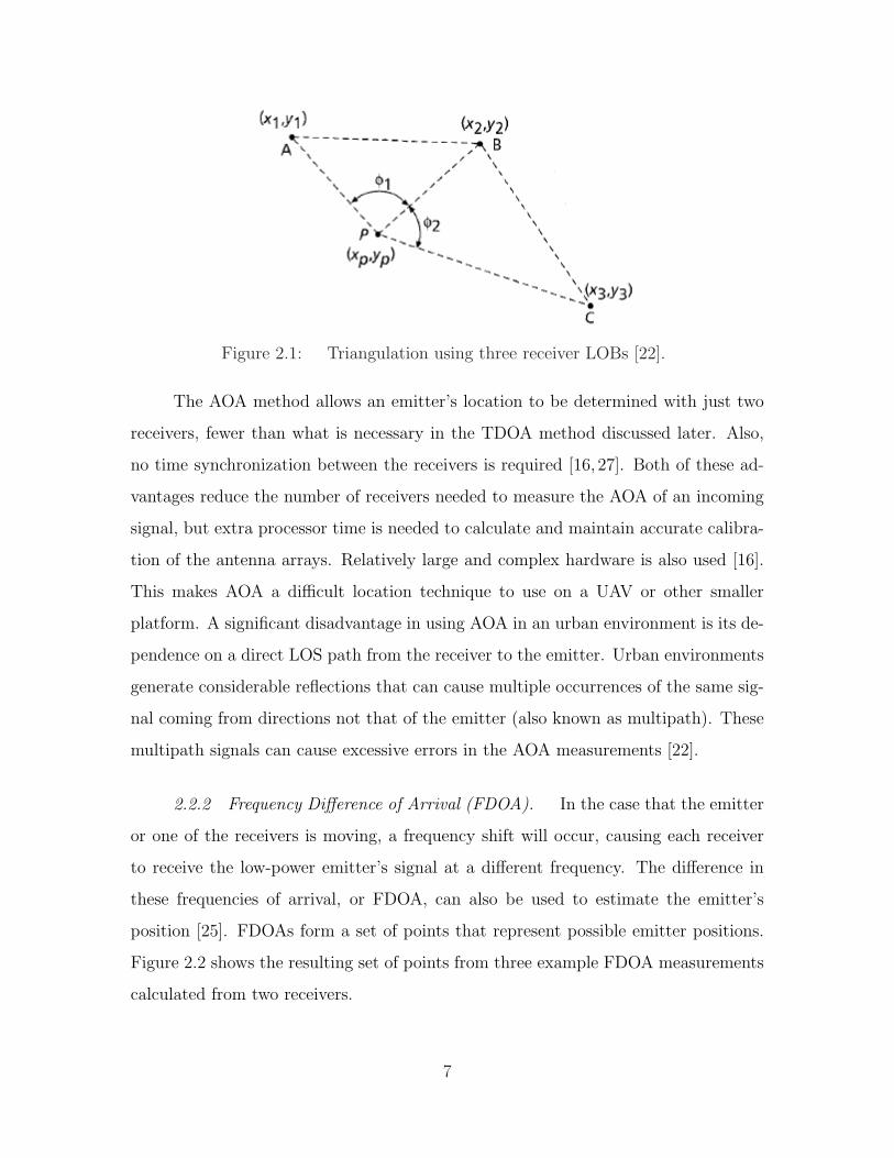
Figure 2.1: Triangulation using three receiver LOBs [22].

The AOA method allows an emitter’s location to be determined with just two

receivers, fewer than what is necessary in the TDOA method discussed later. Also,

no time synchronization between the receivers is required [16, 27]. Both of these ad-

vantages reduce the number of receivers needed to measure the AOA of an incoming

signal, but extra processor time is needed to calculate and maintain accurate calibra-

tion of the antenna arrays. Relatively large and complex hardware is also used [16].

This makes AOA a difficult location technique to use on a UAV or other smaller

platform. A significant disadvantage in using AOA in an urban environment is its de-

pendence on a direct LOS path from the receiver to the emitter. Urban environments

generate considerable reflections that can cause multiple occurrences of the same sig-

nal coming from directions not that of the emitter (also known as multipath). These

multipath signals can cause excessive errors in the AOA measurements [22].

2.2.2 Frequency Difference of Arrival (FDOA). In the case that the emitter

or one of the receivers is moving, a frequency shift will occur, causing each receiver

to receive the low-power emitter’s signal at a different frequency. The difference in

these frequencies of arrival, or FDOA, can also be used to estimate the emitter’s

position [25]. FDOAs form a set of points that represent possible emitter positions.

Figure 2.2 shows the resulting set of points from three example FDOA measurements

calculated from two receivers.

7

Figure 2.2: FDOA contours [25].

The FDOA method has several limitations in its ability to locate low-power

emitters. The relative velocity between the two receivers must be large enough for

the FDOA to outweigh the frequency measurement error [14]. The receivers also

need to have the ability to measure frequency with more accuracy than the smallest

frequency shift that is expected. If this accuracy is not possible, the FDOA may

be undetectable below the noise. FDOA is difficult to implement, and very costly,

especially when the signal is already at a very low power level [25].

2.2.3 Time of Arrival (TOA). Using the time that a signal arrives at a

receiver is another technique that is used in determining the location of an emitter.

Because signals propagate at the constant speed of light, the distance from a trans-

mitter to a receiver can be calculated from the propagation time of the signal [22].

This estimated distance forms a circle around the receiver. The intersection of three

or more of these circles provides an estimate of the location of the emitter.

For the TOA method to work, specific knowledge of the emitter’s signal must

be known. TOA uses precise time synchronization of all the receivers, as well as the

emitter of interest. The exact time the signal left the emitter must be known in order

to determine the signal propagation time [22, 30]. In this research the signal type

8

and waveform are known, but because the timing is unknown, there is no way to

synchronize its time source with each receiver’s time source to obtain the precise time

when the signal left the emitter.

2.2.4 Time Difference of Arrival (TDOA). The TDOA-based approach to

loca-ting emitters is one of the most commonly used position location techniques [30].

TDOA is used in many geolocation, operational and scientific applications [3] and is

widely used in sonar and radar to find the position of a signal of interest [31]. Many

navigation systems, including long range navigation (LORAN) and Decca, use the

TDOA between a radio signal and multiple stations to determine a desired navigation

position [10].

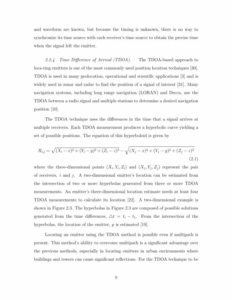
The TDOA technique uses the differences in the time that a signal arrives at

multiple receivers. Each TDOA measurement produces a hyperbolic curve yielding a

set of possible positions. The equation of this hyperboloid is given by

Ri,j =√

(Xi − x)2 + (Yi − y)2 + (Zi − z)2 −√

(Xj − x)2 + (Yj − y)2 + (Zj − z)2

(2.1)

where the three-dimensional points (Xi, Yi, Zi) and (Xj, Yj, Zj) represent the pair

of receivers, i and j . A two-dimensional emitter’s location can be estimated from

the intersection of two or more hyperbolas generated from three or more TDOA

measurements. An emitter’s three-dimensional location estimate needs at least four

TDOA measurements to calculate its location [22]. A two-dimensional example is

shown in Figure 2.3. The hyperbolas in Figure 2.3 are composed of possible solutions

generated from the time differences, 4t = ti − t1. From the intersection of the

hyperbolas, the location of the emitter, p is estimated [19].

Locating an emitter using the TDOA method is possible even if multipath is

present. This method’s ability to overcome multipath is a significant advantage over

the previous methods, especially in locating emitters in urban environments where

buildings and towers can cause significant reflections. For the TDOA technique to be

9

Figure 2.3: TDOA hyperbolic curves [19].

successful, at least one LOS path between the emitter and each receiver must exist.

If there is a LOS path from the emitter to a sensor, and multipath is present, the

signal with the least time delay (as determined by correlation described later) is the

LOS signal [16]. The condition when there is no LOS path between the transmitter

and a receiver is discussed more in Section 2.6.2.

Another advantage in using TDOA to passively locate unknown emitters (over

the other methods presented) is that there is no requirement that the emitter be

synchronized in time with the receivers. When using the TDOA technique to locate

the source of a signal, the time that the signal left the emitter is not needed, and

only the receivers need to be synchronized in time [22, 30]. A timing reference that

is commonly used is global positioning system (GPS), but in urban environments,

access to GPS satellites is often obstructed by buildings or towers. Another approach

that is used in time synchronization is the use of atomic clocks, like a Rubidium

or Cesium time source [16]. The ability to locate a signal using TDOA without

needing to time synchronize the emitter is especially important in detecting signals

passively. In passive detection, the characteristics of the signal coming from the

emitter are unknown, so there is no way to obtain the exact time when the signal left

the emitter [15].

Estimation of an unknown emitter’s position depends on the ability to measure

the time differences of the signal as it arrives at several different receivers. These

10

time difference measurements can be accomplished using time correlation methods

described in the next section.

2.3 Time Difference of Arrival Estimation (TDOA)

Typically two spatially separated receivers will receive the same emitted signal at

different times. An example configuration is shown in Figure 2.4. This configuration

is represented by received signal equations

x(t) = s(t) + nx(t) (2.2)

y(t) = αs(t−D) + ny(t), (2.3)

where s(t) is the original signal, nx(t) and ny(t) are uncorrelated zero-mean Gaussian

noise processes, α is the scaled difference in amplitude between the two received

signals, and D , which can be either positive or negative, is the TDOA between the

two signals [31].

Figure 2.4: Example configuration of two receivers and oneemitter.

After the signal is acquired by the two receivers, correlation analysis is per-

formed. This correlation yields the difference of time that each receiver actually re-

ceived the signal. Several of these time measurements, converted to distance, are used

to calculate the location of the low-power emitter of interest, as previously discussed.

This section reviews two methods that are used to correlate two received signals to

find the TDOA. The cross correlation function can be used when the emitter and the

two receivers are stationary. The complex ambiguity function can be used to estimate

11

both the FDOA and the TDOA for cases when there is motion among the emitter or

the receivers.

2.3.1 Cross Correlation Function. The first step in locating an emitter is

estimating the TDOA. For this research, the signals are assumed to be real-valued. A

commonly used method to obtain this measurement is by using the generalized cross

correlation function

Rxy(τ) = E[x(t)y(t− τ)], (2.4)

where E is the expected value operator.

Figure 2.5 illustrates the process of the cross correlation function when it is

applied to find the TDOA of a signal. Assuming ergodicity, the cross correlation in

(3.2) can generally be written as

Rxy(τ) =1

T − τ

∫ T

τ

x(t)y(t− τ)dt, (2.5)

where T is the observation interval. The value of τ that maximizes the cross corre-

lation function in (3.3) is the time delay estimate, R [15]. A visual example of this is

also shown in Figure 2.6.

Figure 2.5: Correlation of two received signals, x(t) and y(t)to obtain the TDOA.

Error analysis of the cross correlation function shows that adding a filter to

the input of each signal prior to correlation improves the accuracy of the time delay

estimate [15]. In the frequency domain, adding a filter is equivalent to multiplying

the power spectral density by a weighting function. Knapp and Carter [15] describe

five weighting functions that are designed to reduce noise for different cases. Function

12

Figure 2.6: Cross correlation example. R is the estimatedtime delay [11].

selection requires some knowledge of the transmitted signal’s frequency spectrum and

noise [31], which may not be readily available for an unknown signal. But if char-

acteristics like the waveform, or expected signal power are known, using a weighting

function may prove to be beneficial in correlating the signal to find its TDOA.

2.3.2 Correlation Window Size. The ability to correlate two signals also

depends on the autocorrelation of the original signal from the emitter that is being

located. By increasing the correlation window size (Ts), the autocorrelation of a

signal shows a more narrow peak. When the autocorrelation of a signal has a more

narrow, defined peak, the chance for error and ambiguities to occur when correlating

the signal after it is received by two spatially separated receivers is lower than in the

case when the autocorrelation has a wider peak [17]. Various GSM autocorrelation

functions using different correlation window sizes (Ts) are shown in Figure 2.7. In

this figure, Ts is also equal to the total signal length. Increasing the sampling rate

may also benefit correlation of two signals. The correlation window size is especially

important when the emitter produces a low-power signal, causing the SNR to also be

low. This is further developed in Chapter III.

13

Figure 2.7: Auto-correlations of GSM signal with various cor-relation window sizes, Ts [17].

The methods discussed to decrease the chance for ambiguities and errors while

correlating two received signals will have to be balanced with the time and processor

requirements of the geolocation system and its ability to locate an unknown emitter

in the time required.

2.3.3 Ambiguity Function. The ambiguity function is viewed as an extension

of the generalized cross correlation function for moving receivers or transmitters. It

can be used to jointly estimate both the TDOA and FDOA of a signal at two spatially

separated receivers [24]. With the addition of phase shift, the received signals become

14

more complicated, as shown in the equations

x(t) = s(t) + nx(t) (2.6)

y(t) = Ars(t−D)ej2πfdt + ny(t), (2.7)

where fd is the FDOA and D is again the TDOA between the two receivers. The

complex ambiguity function is given as [24]

|A(τ, fd)| =∫ T

0

x(τ)y∗(t− τ −D)e−j2πfdte+j2πfdτdt, (2.8)

where τ corresponds to the estimated TDOA, D. τ and fd are simultaneously solved

to maximize |A(τ, fd)|, resulting in the estimated TDOA and FDOA of the signal

between two receivers [24].

Using both the TDOA and FDOA methods allows the estimate of the emitter’s

location in both poor noise conditions as well as in the presence of many spectrally

and spatially overlapping interfering signals. Figure 2.8 shows a typical complex

ambiguity function in which TDOA and FDOA can be determined [26].

Both the generalized cross correlation function and the ambiguity function suffer

in poor SNR environments. Thus, if implemented techniques discussed previously to

reduce noise at the receivers (filtering) may have to be considered [26], especially for

a low-power emitter.

2.4 Estimation of Low-Power Emitter Location

The previous section described how correlation can be used to estimate the

TDOA between two received signals. Once the TDOA between all pairs of receivers

has been estimated, the location of the low-power emitter can be solved by finding

the intersections of the formed hyperbolas with respect to the known receiver loca-

tions, as discussed earlier. But because the equations of the hyperbolas are nonlinear,

estimating the solution through brute force calculations can be time consuming and

15

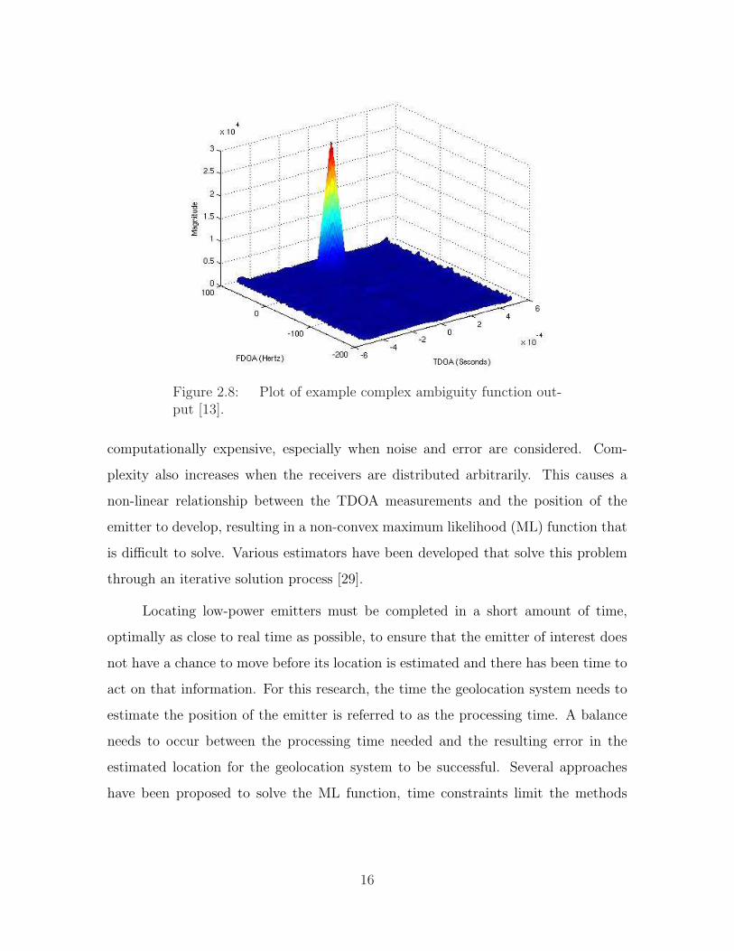
Figure 2.8: Plot of example complex ambiguity function out-put [13].

computationally expensive, especially when noise and error are considered. Com-

plexity also increases when the receivers are distributed arbitrarily. This causes a

non-linear relationship between the TDOA measurements and the position of the

emitter to develop, resulting in a non-convex maximum likelihood (ML) function that

is difficult to solve. Various estimators have been developed that solve this problem

through an iterative solution process [29].

Locating low-power emitters must be completed in a short amount of time,

optimally as close to real time as possible, to ensure that the emitter of interest does

not have a chance to move before its location is estimated and there has been time to

act on that information. For this research, the time the geolocation system needs to

estimate the position of the emitter is referred to as the processing time. A balance

needs to occur between the processing time needed and the resulting error in the

estimated location for the geolocation system to be successful. Several approaches

have been proposed to solve the ML function, time constraints limit the methods

16

that can be used to estimate the emitter’s location. Those methods that may cut

down processor time are discussed in this section.

2.4.1 Taylor Series Approximation. One of the simplest methods to find a

solution of hyperbolic TDOA equations is to use a Taylor-series expansion to linearize

the hyperbolic equations. Although commonly used, this method needs an initial

guess close to the true solution to avoid being stuck in a local minima. It also improves

the location estimate in a series of steps, determining the local linearization solution

(LS) at each step. There is no guarantee of convergence to a solution, especially when

the initial guess is not close to the true solution [4,12]. Because little is known about

the emitter of interest, it would be difficult to guess the initial location required to

estimate the position, especially if this were implemented on an automated system

without a human decision maker. Also, calculating the LS during each estimation

step adds to the calculations that are needed and processor time. This added time

may limit the geolocation system’s ability to locate an emitter in near-real time.

2.4.2 Closed-Form Solution. Another method of estimating the location

of an emitter from TDOA measurements is a closed-form technique. In comparison

to other emitter location estimation methods, closed-form methods may not be as

accurate. Chan and Ho [4] have developed a closed-form solution that can be used

to determine an emitter’s location for both near and far sources. This method only

works when the signal has a large SNR, and the number of receivers must be four.

Fang [10] developed a method that estimates a unique position for the case when the

number of TDOA measurements is equal to the number of unknown coordinates to

the emitter. Most closed-form solutions, although they require less calculations than

the Taylor-series expansion method, cannot take advantage of extra receivers that

may improve solution accuracy [4].

2.4.3 Hyperbolic Asymptotes. An additional method of localization using

TDOA measurements has been developed that is less computationally intensive, but

17

may also be less accurate than the previous estimation methods referenced. Drake

and Dogancay [9], proposed a new, simplified method to locate an emitter by using the

set of linear equations that corresponds to the hyperbolic asymptotes of the TDOA

measurements.

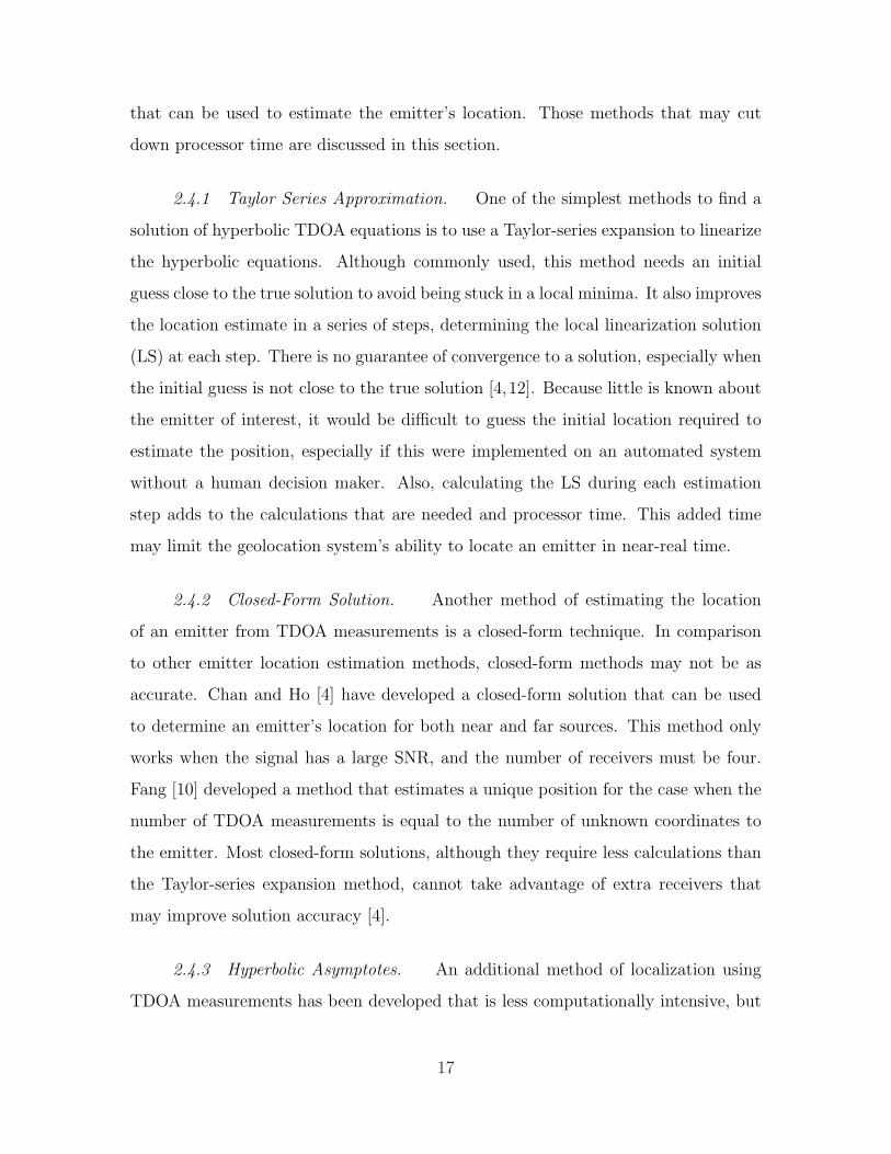
Figures 2.9 and 2.10 show hyperbolas and their respective hyperbolic asymp-

totes [9]. This method of estimating an emitter’s location reduces the calculations

needed considerably. However, it also introduces more room for error, especially if

the receivers are relatively close to the emitter, or to each other.

Figure 2.9: Geolocation using TDOA hyperbolas [9].

2.5 Over-Approximation

Because LOS signal paths to the emitter are more difficult to obtain in an urban

environment, more receivers than are minimally required to estimate a position must

be deployed, so more TDOA measurements may be obtained than are necessary to

estimate the emitter’s position. But some receivers may be further from the emitter

than others, or there may not be a direct path from a receiver to the emitter, which

could add more uncertainty to the estimated location. There are a few estimation

18

Figure 2.10: Geolocation using hyperbolic asymptotes [9].

methods that take into account extra TDOA measurements. One of these methods

is the Divide and Conquer (DAC) approach.

2.5.1 Divide and Conquer Position Estimation Method. The DAC estima-

tion method divides the TDOA measurements into equal groups each containing the

same number of unknowns. The unknown parameters are calculated in each group,

then combined to give the final position estimate [2]. This solution uses stochastic

approximation and requires a large amount of data, which limits the amount of noise

that can be tolerated [4]. This is a significant disadvantage in estimating the location

of a low-power signal, where the noise level may be relatively high compared to the

signal power. This method also assumes that the receivers have a good LOS signal

path to the emitter, and all TDOA measurements are good. It does not distinguish

between measurements taken from a receiver close to the emitter and one that may

be further away that may cause more error in its relative TOA measurements.

2.5.2 Linear Weighted Least Squares (WLS) Algorithm. In real environ-

ments, TDOA measurements contain noise, either from inconsistencies in the re-

ceivers, or from other outside sources. Torrieri [28] derived the principal algorithms

19

in 1984 that are still commonly used to estimate an emitter’s position from TDOA

measurements [29]. Torrieri’s weighted least squares (WLS) estimator, when applied

to finding the location of an emitter using TDOA measurements, can successfully

compute a location estimate from any number of sensors and their respective TDOA

measurements.

The location of an emitter is estimated from TDOA measurements using an

iterative linear WLS approach. WLS is an estimation method that is similar to the

more common LS method. The WLS estimation method uses the same minimization

of the sum of the residuals:

S =n∑

i=1

[yi − f(xi)]2, (2.9)

where (xi, yi) are the data points for i = 1, 2, ..., n cases. For position estimation

using TDOA, the TDOA values and sensor location information serve as the input

data points. The function f that produces f(xi) ≈ yi + εi gives the solution, an

estimated emitter position.

The WLS method of estimation is similar to the LS approach, but instead of

weighting all the points equally as in (2.9), the points are weighted such that the

points with a greater weight contribute more to the fit:

S =n∑

i=1

wi[yi − f(xi)]2. (2.10)

The weight, wi, is usually given as the inverse of the variance, giving points with a

lower variance a greater statistical weight [28]:

wi = 1/σ2i . (2.11)

Applying this WLS method may cut down on the number of iterations needed

for the solution to converge because there will be less variance in each estimate, further

reducing the overall time the processor needs to make all the calculations. But as the

20

number of sensors and their respective TDOA measurements increase, the number of

calculations needed will rise, increasing the processing time.

As the methods presented in this section suggest, over-approximation still re-

mains a problem in locating the source of a signal. A new estimation method that

takes advantage of additional TDOA measurements than are necessary is developed

in Chapter III.

2.6 Urban Environment Characteristics

In a dense urban environment, there may not always be direct LOS from a

receiver to the emitter of interest. Buildings and towers can cause the signal to be

blocked or reflected, causing multiple paths to occur. Figure 2.11 shows an example

of several receivers and the respective signal paths to an emitter of interest.

Figure 2.11: Example layout of receivers and emitter in anurban environment with possible signal propagation paths dis-played. City background from [1].

2.6.1 Multipath. As discussed earlier, assuming that a direct LOS exists

between the receiver and emitter, when multiple delayed copies of the signal arrive

at a specific receiver, also known as multipath, the signal with the least time delay

is the LOS signal [16]. The LOS path is assumed to be the most direct path to the

emitter [22]. Figure 2.12 shows an example of how the same signal can be received

multiple times at one receiver.

21

Figure 2.12: Example of multipath signals.

2.6.2 Non-Line of Sight (NLOS). In locating an emitter, position error and

complexity is added if an obstacle like a building or tower blocks the LOS path between

the sensor and emitter. In this case, the most direct signal path from the emitter to

the sensor is not the LOS path, leading to error and variance in the estimated position

of the emitter. Non-LOS (NLOS) paths from the emitter to the sensors are common,

especially in the urban environment. There is a great need to have the ability to

determine which sensor in a geolocation system is limited to a NLOS path from the

emitter. If the NLOS sensor can be identified and removed from the system, the

error associated with this sensor’s TDOA calculations can also be removed, leading

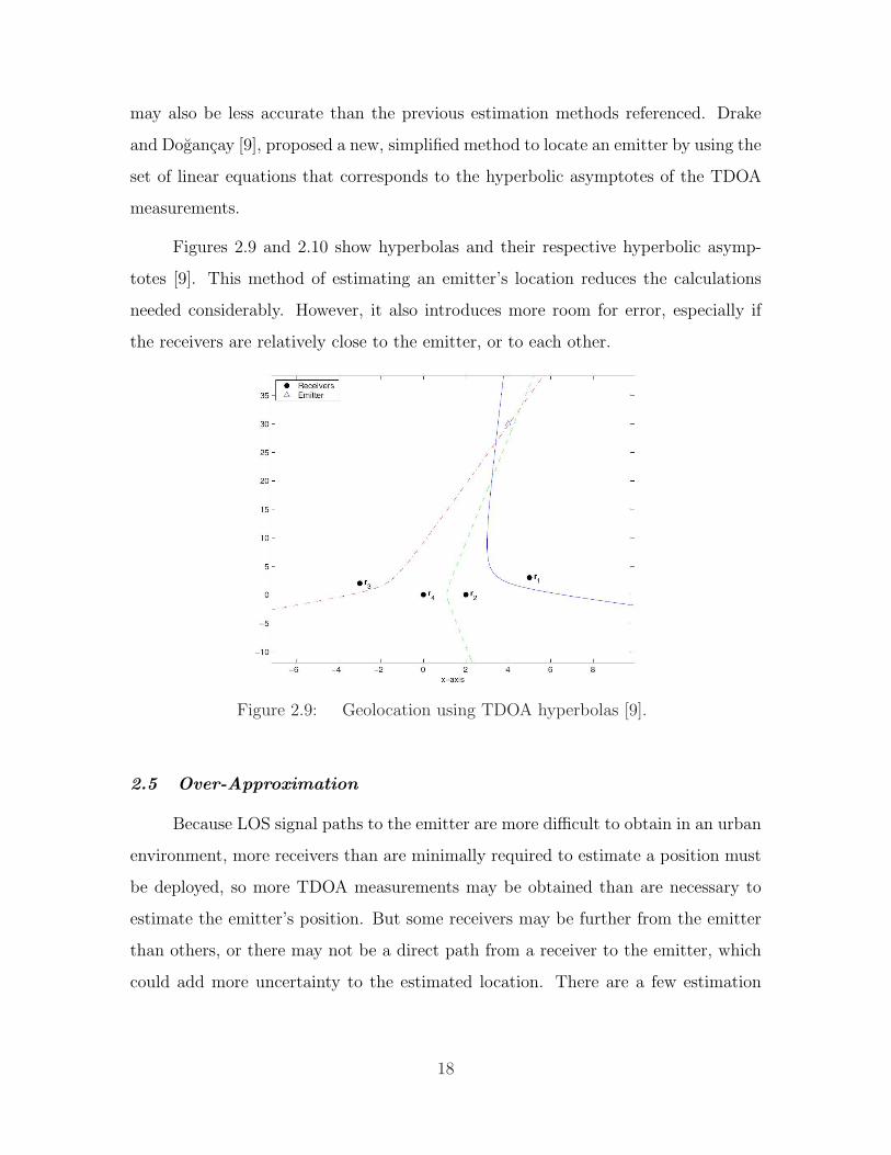
to a more accurate emitter position estimate [7]. Figure 2.13 shows an example

configuration that includes a NLOS receiver.

Identifying a NLOS sensor is crucial in reducing the error in estimating the

position of a low-power emitter. If a sensor has a NLOS propagation path to the

emitter, the signal has to travel a longer distance to reach the sensor. This causes the

estimated position to be further away from the NLOS sensor and away from the true

position of the emitter. Figure 2.14 shows the effect a NLOS receiver can have on the

overall TDOA position estimate. In this configuration, the mobile station (MS) is the

emitter, and each base station (BS), is a sensor.

22

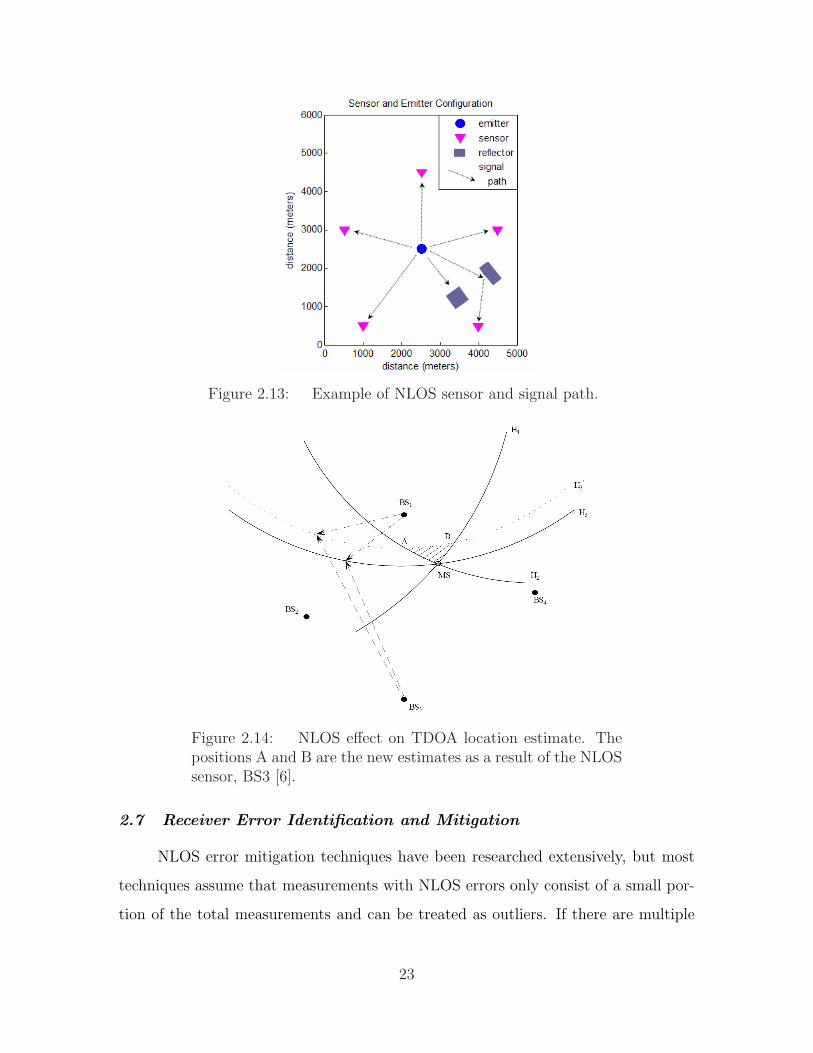
Figure 2.13: Example of NLOS sensor and signal path.

Figure 2.14: NLOS effect on TDOA location estimate. Thepositions A and B are the new estimates as a result of the NLOSsensor, BS3 [6].

2.7 Receiver Error Identification and Mitigation

NLOS error mitigation techniques have been researched extensively, but most

techniques assume that measurements with NLOS errors only consist of a small por-

tion of the total measurements and can be treated as outliers. If there are multiple

23

NLOS sensors present, these measurements make up a larger portion of the total

measurements, and can have a much larger effect on the final estimated position [7].

Several error mitigation methods using deletion diagnostics have been developed

to work around the problem of multiple NLOS receivers. The time-history based

approach and the method of ranking the residual of each receiver have both been

adopted by many to reduce the effect a NLOS receiver may have on the overall

emitter position estimate. There is also research into how the geometrical layout

of the sensors affects the estimated position of the emitter of interest. This section

describes these methods.

2.7.1 Time-History Based Approach. Wylie and Holtzman [32] developed

a time-history based hypothesis test that identifies the NLOS error in TDOA calcu-

lations by looking at each base station’s relative TOA measurement over a period

of time, then combining this information with the variance of the standard noise

measurement. Their work was focused on cell phone systems.

This NLOS identification technique then compares the standard deviation of

a sample statistic (each base station’s relative TOAs and the known standard noise

for each receiver) to the known standard deviation of that statistic when the mea-

surements are from a LOS receiver. When there is a LOS from the base station to

the MS, then the standard measurement noise’s effect on the measured TOA can be

predicted. If there is NLOS error present, then the measured TOA is expected to

have a significantly larger average deviation from the expected curve than when there

is no NLOS error present [32]. This method works well to detect if a receiver has only

a NLOS signal path to the emitter, but cannot differentiate which receiver has the

NLOS signal path.

2.7.2 Residual Ranking. One general method adopted by many researchers [5,

32] uses a residual rank test. In this method, all of the initial relative TOA measure-

ments, ti, are used to estimate the emitter’s position. A NLOS error in a receiver

24

can cause inconsistent TOA measurements, leading to inconsistencies in the TDOA

calculations as well. After several emitter position estimates are completed over time,

the NLOS error will become more detectable due to its irregularities.

A residual rank test can be performed to determine which receiver is most likely

to have the NLOS signal path to the emitter. The general steps are:

1. Use all TDOA measurements at ti to estimate the position.

2. Calculate each receiver’s residual:

em(ti) = rm(ti)− Lm(ti), (2.12)

where rm(ti) represents the measured TDOAs, and Lm(ti) = |d(ti)−dm| are the

calculated TDOAs.

3. Count number of times |em(ti)| is largest error for each ti.

4. Rank results from 3.

The receiver with the consistently largest residual, em(ti), is assumed to be the re-

ceiver with the NLOS signal path to the emitter [32]. This method is effective in

determining if there is a NLOS receiver, but needs several position estimates over an

extended period of time to allow the NLOS receiver’s relative TOA measurements

have a detectable effect on the overall position estimate of the emitter. While effec-

tive, this method may take too much time to allow for near-real time emitter position

estimates. This also does not account for the case of more than one NLOS receiver.

2.7.3 Receiver Geometrical Layout. Because of the recent government push

towards E-911, most research into passively locating emitters assumes a typical cell

phone BS geometrical configuration. In this layout, the cell phone emitter is sur-

rounded by BS’s that are evenly spaced azimuthly around the cell phone [7]. An

example of this is in Figure 2.15.

25

Figure 2.15: BS typical layout [7].

More recently, Drake [8] explored receiver geometrical layouts as they would

happen if mounted on multiple UAVs. Using statistical analysis developed by Torri-

eri [28], Drake was able to accurately predict error bounds for various receiver layouts.

These are shown in Figures 2.16a and 2.16b.

If the receivers are mounted on UAVs, the ability exists to move the receiver

that is causing the error to help mitigate the multipath NLOS error. If a sensor is

identified as located in a poor location with respect to the other sensors, causing

more error in the estimated position of the emitter, that sensor can be moved to a

better location. Based on the error predictions of various sensor configurations, better

sensor geometrical layouts can be recommended and implemented while the UAVs are

in flight, assuming that an initial position estimate can be obtained.

Techniques of identifying a NLOS receiver work well when there is only one

receiver with a NLOS path from the emitter and the sensors are located surrounding

the emitter [7]. But many times more than one BS suffers from NLOS, or more

than one receiver is located too far away from the emitter to help in estimating the

emitter’s location. The case when more than one receiver contributes to bad TDOA

measurements is further developed in Chapter III.

26

Figure 2.16: TDOA location uncertainty elipses for good (a)and poor (b) geometry [8].

2.8 Summary

This chapter provides a foundation on geolocation systems, reviewing several

methods that can be used to locate signal sources, specifically, those methods that

can be applied to passively locate low-power emitters. The TDOA emitter locating

technique is the most appropriate method to find the source of a low-power signal. It

is less computationally intensive and physically less complex than the AOA and TOA

methods. For these reasons, TDOA was the method of choice for this research.

There are several major challenges in developing methods to passively locate

low-power emitters. Size, weight, power and cost all have important roles and are

considered in the design of the hardware and algorithms of the geolocation system.

27

Many approximation methods that are used to estimate the location of a signal from

TDOA measurements are explored, but none fit the constraints of deploying the

system onto a UAV or other smaller platform. A combination of these techniques

is required to successfully locate low-power emitters, and will have to be developed

to meet these strict limitations. Chapter III includes simulation methodology for

a robust geolocation system that can locate a low-power emitter in the presence of

multipath using multiple receivers, one of which only has a NLOS path to the emitter.

28

III. Simulation Methodology

3.1 Overview

This chapter provides a description of the simulations developed for this research

to include the structure of the algorithms developed and used. An overall system

description is presented followed by a detailed description of each system component

and how each component is used in locating the emitter of interest.

3.2 Geolocation System

The proposed passive geolocation system is comprised of several parts: a) the

sensors, b) the correlators, c) WLS position estimator, d) a NLOS sensor detection

and identification algorithm and finally, e) a sensor redirection algorithm. The bulk

of this research effort was spent on the identification and mitigation of NLOS sensors.

Figure 3.1 shows an example sensor and emitter configuration and the true and

estimated positions of the emitter of interest. This is a simple case where each sensor

has a LOS propagation path from the emitter and the sensors encompass the emitter.

Figure 3.1: Example receiver configuration with estimatedand true emitter positions. All sensors have a LOS signal pathto the emitter.

29

In urban environments where buildings and towers are common, there is a need

to identify when the LOS path from the emitter to the sensor is blocked. If a sensor’s

LOS path is blocked or reflected, the signal it receives is delayed, causing the time that

the signal arrives at the sensor to be later than if the signal propagated directly to the

sensor. This is the result of the signal reflecting off other buildings and obstacles before

it reaches the receiving sensor. When this received signal is included in the geolocation

solution, any TDOA calculation and resultant position estimate will include additional

error. To estimate the position of the low-power emitter accurately, the source of

this error needs to be determined and removed from the geolocation system. After

the sensor is removed from the geolocation system, the emitter location can be re-

estimated more accurately without the added NLOS error. Figure 3.2 shows a top-

level view of the geolocation system.

Figure 3.2: Passive geolocation system.

3.3 Sensor Parameters

The geolocation system includes N sensors that each receive the signal of in-

terest. It is assumed that the sensors each have identical capabilities. Each sensor

is omni-directional and can detect and receive the signal coming from the low-power

emitter. All sensors have perfect timing and are synchronized.

30

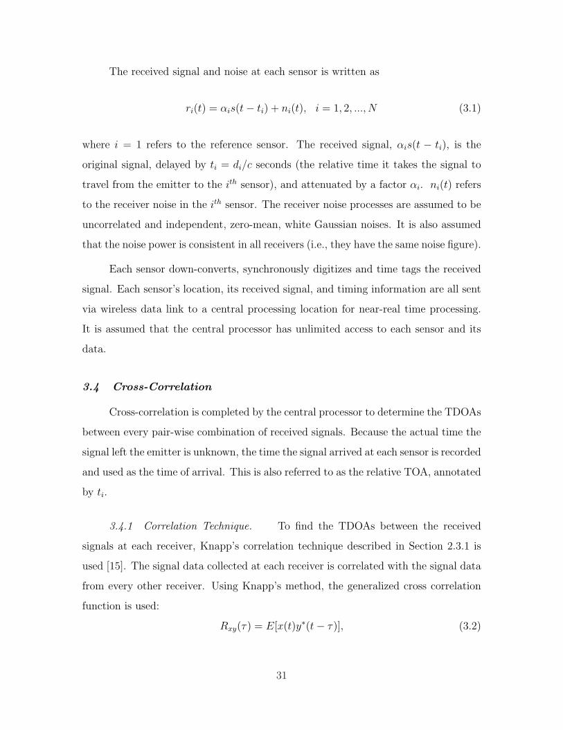
The received signal and noise at each sensor is written as

ri(t) = αis(t− ti) + ni(t), i = 1, 2, ..., N (3.1)

where i = 1 refers to the reference sensor. The received signal, αis(t − ti), is the

original signal, delayed by ti = di/c seconds (the relative time it takes the signal to

travel from the emitter to the ith sensor), and attenuated by a factor αi. ni(t) refers

to the receiver noise in the ith sensor. The receiver noise processes are assumed to be

uncorrelated and independent, zero-mean, white Gaussian noises. It is also assumed

that the noise power is consistent in all receivers (i.e., they have the same noise figure).

Each sensor down-converts, synchronously digitizes and time tags the received

signal. Each sensor’s location, its received signal, and timing information are all sent

via wireless data link to a central processing location for near-real time processing.

It is assumed that the central processor has unlimited access to each sensor and its

data.

3.4 Cross-Correlation

Cross-correlation is completed by the central processor to determine the TDOAs

between every pair-wise combination of received signals. Because the actual time the

signal left the emitter is unknown, the time the signal arrived at each sensor is recorded

and used as the time of arrival. This is also referred to as the relative TOA, annotated

by ti.

3.4.1 Correlation Technique. To find the TDOAs between the received

signals at each receiver, Knapp’s correlation technique described in Section 2.3.1 is

used [15]. The signal data collected at each receiver is correlated with the signal data

from every other receiver. Using Knapp’s method, the generalized cross correlation

function is used:

Rxy(τ) = E[x(t)y∗(t− τ)], (3.2)

31

where E [ ] is the expected value operator. This equation, assuming ergodicity, can be

written as

Rxy(τ) =1

t− τ

∫ T

τ

x(t)y∗(t− τ)dt, (3.3)

where T is the observation interval. The value of τ that maximizes this cross corre-

lation function is the TDOA estimate, ti − ti+1 [15].

The TDOAs between each pair-wise combination of receivers is estimated using

the cross-correlation function in (3.3). Figure 3.3 displays the hyperbola set of solu-

tions that can be drawn from calculated TDOAs between three simulated receivers

located at “x.” The estimated emitter location (*) lies at the intersection of the

hyperbolas.

0 500 1000 1500 2000 2500 3000 3500 4000 4500 50000

500

1000

1500

2000

2500

3000

3500

4000

4500

5000TDOA Hyperbolas

distance

dist

ance

Figure 3.3: Estimated TDOA hyperbolas for three receiverslocated at “x.”

3.4.2 Correlation Window. The correlation window size will affect the ac-

curacy of the TDOA estimation. As Figure 3.4 shows, the peak of the autocorrelation

of a modeled BPSK signal varies in width with respect to the correlation window.

The BPSK signal parameters used in simulation are described in Section 3.7.1. Side

lobes in the autocorrelation of a signal can indicate possible sources of error while

32

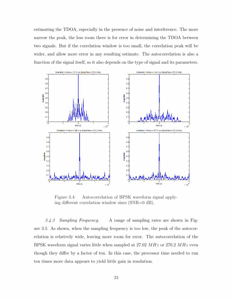
estimating the TDOA, especially in the presence of noise and interference. The more

narrow the peak, the less room there is for error in determining the TDOA between

two signals. But if the correlation window is too small, the correlation peak will be

wider, and allow more error in any resulting estimate. The autocorrelation is also a

function of the signal itself, so it also depends on the type of signal and its parameters.

Figure 3.4: Autocorrelation of BPSK waveform signal apply-ing different correlation window sizes (SNR=0 dB).

3.4.3 Sampling Frequency. A range of sampling rates are shown in Fig-

ure 3.5. As shown, when the sampling frequency is too low, the peak of the autocor-

relation is relatively wide, leaving more room for error. The autocorrelation of the

BPSK waveform signal varies little when sampled at 27.02 MHz or 270.2 MHz even

though they differ by a factor of ten. In this case, the processor time needed to run

ten times more data appears to yield little gain in resolution.

33

Figure 3.5: Autocorrelation of BPSK waveform signal aftervarious sampling rates are used (SNR=0 dB).

3.4.4 Smoothing Function. Because there may be some noise in the signal,

especially at lower power levels, the cross correlations are smoothed using a smoothing

function. The smoothing function performs a moving average of a specified number

of correlated points (Ns). An example of this can be seen in Figure 3.6 for Ns = 8.

Eight was used as the moving average window because it produced results consistent

with the desired ten meter estimated position solution resolution.

3.4.5 Resolution. As discussed in previous sections, precision of the es-

timated position is affected by the size of the correlation window and the rate of

sampling. Increasing the correlation window size may increase the precision of the

cross-correlation calculations, but a larger correlation window also adds more data

points to process, adding to the overall processing time the system needs to estimate

the position of the emitter. Increasing the sampling rate can also increase the resolu-

tion of the position estimate, but this also adds more processing time. Both methods

34

−5000 −4000 −3000 −2000 −1000 0 1000 2000 3000 4000 50000

0.2

0.4

0.6

0.8

1Cross Correlation before Smoothing

samples

ampl

itude

−5000 −4000 −3000 −2000 −1000 0 1000 2000 3000 4000 50000

0.2

0.4

0.6

0.8

1Cross Correlation after Smoothing

ampl

itude

samples

Figure 3.6: Smoothing function (Ns = 8): autocorrelationof BPSK signal before and after smoothing function is imple-mented.

of increasing the resolution of the estimate reach a point when adding more data

points no longer adds to the precision of the estimate.

The correlation window size depends on the signal that is being correlated. For

example, the GSM cell phone uses time division multiple access (TDMA) to optimize

communication channels, where each time division is 577 µs long. To accommodate

this, the GSM signal is sent in 577 µs long pulses every eight time divisions. For this

case, using a correlation window longer than 577 µs would not be favorable because it

would cause the geolocation system to spend unnecessary processing time correlating

noise and interference while no signal is being sent. Section 3.7.2 provides more detail

on the GSM cell phone signal characteristics.

For all results and analysis in this research, a correlation window of 144.2 µs is

chosen to find each estimated TDOA. This is shorter than a GSM signal pulse but

provides the desired resolution in the position estimate. Several different correlation

windows and their effects on the estimated position variance and error of the emitter

are explored in Chapter IV. The correlation window size and sampling rate will need

35

to be re-evaluated if the geolocation system is used to locate an emitter with a different

signal waveform than is presented here.

The sampling rate can limit the resolution of the estimated position. For ex-

ample, a sampling rate of 72.02 MHz results in 100 samples per 3.7 µs symbol, or

1 sample per 37 ns. If the signal travels at the speed of light, c = 3.00 × 108m/s,

one sample will be taken every 11.1 meters. This corresponds to the geolocation sys-

tem having a best possible resolution of 11.1 meters at that sampling rate. Table 3.1

includes possible sampling rates and their impact on the estimated position resolution.

Table 3.1: Signal sampling parameters.Samples/ Sampling Sampling PossibleSymbol Interval Frequency Resolution

(nsec) MHz (m)10 369 2.70 11120 185 5.41 55.640 92.3 10.8 27.7100 36.9 27.1 11.1200 18.5 54.0 5.54

The geolocation system needs to have the ability to locate an emitter in near-real

time while keeping the estimate as accurate as possible. Therefore a balance between

the resolution of the position estimate and the time required by the processor to gain

that resolution needs to be met.

3.5 Position Estimation Using WLS Estimator

A method of estimating the location of a signal source from TDOA measure-

ments is presented that takes advantage of extra receiver TDOA measurements. This

method detects and identifies sensors that provide poor relative TOA measurements

due to NLOS error or low signal power. This is done by using a combination of several

proven location estimation schemes including Residual Ranking and a Weighted Least

Squares Estimation method that were detailed in Chapter II [6, 7].

36

The TDOA measurements found previously through cross correlation are used

to estimate a location. As Figure 3.2 showed, the TDOA measurements between

the sensors along with an initial guess of the emitter position are inputted into Tor-

rieri’s WLS location estimation algorithm [28]. Figure 3.7 displays the geometrical

configuration referred to by the WLS position estimator.

Figure 3.7: Geometry of emitter and N sensors [28].

This algorithm, like most other estimation algorithms, needs an initial position

guess to estimate the position from TDOA measurements. Because the proposed

geolocation system is passive, it is not known initially what area the emitter may be

in, so the centroid, or arithmetic mean between the receivers, R0 = [x, y, z], is used

as the initial position guess.

The distance from sensor i, si, to the reference location, R0, is defined as the

scalor

D0i = ‖R0 − si‖, (3.4)

where si is the matrix containing the known locations of each sensor. The matrix

of derivatives evaluated at the coordinates of the reference location, F, is calculated

from (3.4) as

F =

(R0 − s1)T /D01

(R0 − s2)T /D02

...

(R0 − sN)T /D0N

(3.5)

37

By estimating the TDOAs between each sensor, the initial time the signal left

the emitter, t0, is not needed. The TDOA measurements are written as

ti − ti+1 = (Di −Di+1)/c + ni, i = 1, 2, ..., N, (3.6)

where ni is the measurement error and ti − ti+1 is the difference in time the signal

arrived at each ith sensor. To simplify calculations in Matlabr, (3.6) is written in

matrix form

Ht = HD/c + Hε, (3.7)

where t, D, and ε are N -dimensional column vectors with components ti, Di and

εi. ε refers to the arrival time measurement error, which accounts for propagation

anomalies, receiver noise, and errors in the sensor positions. The H matrix, (N −1)×N is given as [28],

H =

1 −1 0 · · · 0 0

0 1 −1 · · · 0 0...

......

......

0 0 0 · · · 1 −1

.

The final equation for the weighted least squares estimator then becomes [28]

R = R0 + c(FTHTN−1HF)−1FTHTN−1(Ht−HD0/c), (3.8)

where N denotes the covariance matrix of the arrival-time errors. It is defined as

N = HNεHT . (3.9)

38

where Nε represents the estimated noise in the receivers,

Nε =

σ21 0 . . . 0

0 σ22 . . . 0

......

...

0 0 . . . σ2N

, (3.10)

and σ2i is the arrival-time variance.

During each iteration of the LS algorithm, the position estimate and TDOA

estimates are used to generate a new position estimate for the emitter. This position

estimation method continues until the position estimate converges to a location or

the algorithm loop is stopped. To determine if the position estimate has converged

to a solution, the standard deviation, s, is used

s =

√√√√ 1

n− 1

n∑j=1

(Rj − R)2, j = 1, 2, ..., n (3.11)

where Rj refers to the jth iteration of the position estimate, and R refers to the mean

of the estimated locations.

Initial runs of the WLS estimator shows that when the estimate converges to

a solution, it does so over just a few iterations of the estimator. By comparing

the last three estimates the WLS algorithm produces, it can be determined if the

algorithm has converged to a solution, or if more iterations of the WLS estimator

are needed. This saves precious processor time by eliminating redundant position

estimates. Comparing more than the last three estimates yields a position estimate

with no less error than comparing just the last three, and takes more time to run since

more calculations are needed. Standard deviation is used to compare the last three

position estimates. If it is found that the position estimates are within ten meters

of each other, it is assumed that the solution has converged, the WLS estimator is

stopped, and the last position estimate is used as the final estimate out of the WLS

39

estimator. Ten meter resolution is consistent with the initial standards set for this

research in Chapter I. Depending on where the emitter is in relation to the sensors,

it may take several iterations of the WLS estimator to converge to a solution. An

example of an estimated location using this method is shown in Figure 3.8. In this

case, it took five iterations of the WLS location estimator to converge to a solution

close to the true location of the emitter.

Figure 3.8: Estimated position using Torrieri’s method [28].The numbered estimated positions correspond to the order ofiterative emitter location estimates calculated, eventually con-verging close to the true emitter location (SNR = 0).

3.6 Detection and Identification of NLOS Receiver(s)

As mentioned throughout this research effort, there are many challenges in lo-

cating a emitter like a cell phone or walkie-talkie in an urban environment. Besides

the low-power signal levels involved, there are buildings, highways, and towers that

could be in the way of a sensor that is trying to detect and locate the emitter. Since it

is not known exactly where the emitter of interest is, the geolocation system must be

40

able to determine if one of its sensors does not have a LOS propagation path from the

emitter. Therefore, a proposed method of identifying a NLOS receiver is presented.

3.6.1 Approach. Figure 3.9 displays the flow chart for this segment of the

geolocation system.

Figure 3.9: Bad sensor detection and identification process.

The equation

N −K ≥ L, (3.12)

is used to describe how many LOS and NLOS sensors there are, where N is the total

number of sensors, K is the number of NLOS sensors, and L is the minimum number

of LOS sensors required to estimate a position. In 2D position estimation, L = 3 LOS

sensors are needed to estimate a position.

Assuming there are sufficient sensors that have a LOS propagation path to the

emitter, just one emitter position estimate calculated with the WLS estimator is

needed for the Sensor Error Mitigation Algorithm to determine if a sensor adds too

much variation to the estimated emitter position. The sensor may only have a NLOS

path from the emitter and needs to be moved to another location with a LOS path

41

to the emitter to further optimize the position estimate. After the K NLOS sensors

are removed from the computations, an improved emitter location estimate can be

calculated using only the N −K LOS sensors, assuming there still remains at least L

sensors remaining.

3.6.2 Sensor Error Mitigation. Adding more receivers to the geolocation

system does not always increase accuracy in the emitter location estimate. If a receiver

is added to the system, but has only a NLOS signal propagation path to the emitter,

more processor time is needed to identify this bad receiver and to omit it from the

geolocation system. The effects of propagation also play a role in increasing the

amount of error due to the added noise and decrease in signal strength.

It is assumed for the scope of this research that the number of sensors with a

LOS signal path to the emitter is equal to or greater than the minimum required to

estimate a location, L. As mentioned earlier, to determine a two dimensional emitter

location, the minimum number of sensors needed is L = 3. If there are more sensors

than are minimally required to estimate a location (N > L), there is more flexibility

in how the TDOA calculations are grouped and used in the WLS location estimator.

For example, if there are N = 5 sensors, there are 16 different combinations that can

be used to estimate the emitter location.

1. Select 5 out of 5:(55

)= 1 possible combination


)= 5 possible combinations


)= 10 possible combinations

Applying the WLS estimator to these combinations results in 16 different emitter

location estimates. These estimates are referred to as intermediate location estimates.

Because these intermediate location estimates result from different combinations

of sensor TDOA calculations, each estimate will have varied weights of each sensor’s

relative TOA information contributing to it. If there is a NLOS sensor, some of the

position estimates will contain NLOS errors, and others may have fewer or no NLOS

42

errors. These errors depend on which sensor has the NLOS signal path from the

emitter and can result in measurable variance in the estimated intermediate positions.

3.6.3 Emitter Position Variance. If the number of sensors in the geolocation

system is small, a NLOS sensor may cause more error and variance in the estimated

position of the emitter than if the number of sensors is large. For example, if there are

N = 5 sensors, and 1 sensor has a NLOS propagation path to the emitter, the NLOS

sensor will cause there to be some variation and error in the position estimate. But

if there are only N = 3 sensors, and 1 is a NLOS sensor, the variance of the resulting

position estimate is expected to be larger than in the N = 5 case described.

3.6.3.1 Variance Calculation. A plot of the intermediate estimated

positions of a geolocation system that has a NLOS sensor is shown in Figure 3.10.

Each intermediate position plotted represents the result of the WLS estimator after

three sensors and their respective TDOA calculations are used. The variance of

these intermediate location estimates is calculated and plotted for different cases to

determine what the variance is when there is a NLOS sensor in the system.

By using only L sensors’ relative TOA measurements in the WLS algorithm, the

time needed to calculate the position estimate is much less because of the decrease in

matrix calculations needed. If there are N = 5 sensors, as mentioned in Section 3.6.2,

there is just one possible way to select all five sensors at once, and ten possible ways

to select three sensors. Using the WLS method described earlier to estimate the

emitter’s position, one position can be estimated using all five sensor locations and

their respective TDOA information, while ten positions can be estimated by using

each combination of three sensors,(53

), and their respective TDOA information into

the WLS estimator.

Although it may seem to be more efficient to only run the estimator one time, in-

putting 5 arguments 1 time takes approximately the same amount of time to estimate

a position as inputting 3 arguments 10 times. The ability to run more WLS estimates

43

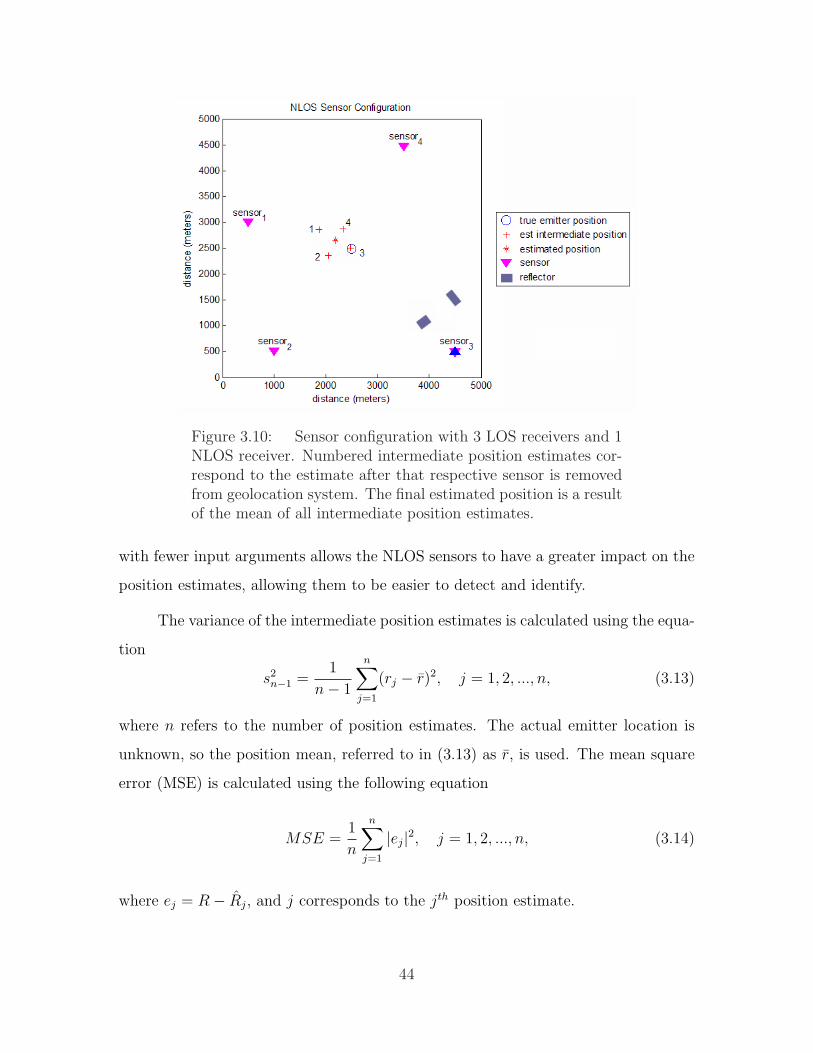
Figure 3.10: Sensor configuration with 3 LOS receivers and 1NLOS receiver. Numbered intermediate position estimates cor-respond to the estimate after that respective sensor is removedfrom geolocation system. The final estimated position is a resultof the mean of all intermediate position estimates.

with fewer input arguments allows the NLOS sensors to have a greater impact on the

position estimates, allowing them to be easier to detect and identify.

The variance of the intermediate position estimates is calculated using the equa-

tion

s2n−1 =

1

n− 1

n∑j=1

(rj − r)2, j = 1, 2, ..., n, (3.13)

where n refers to the number of position estimates. The actual emitter location is

unknown, so the position mean, referred to in (3.13) as r, is used. The mean square

error (MSE) is calculated using the following equation

MSE =1

n

n∑j=1

|ej|2, j = 1, 2, ..., n, (3.14)

where ej = R− Rj, and j corresponds to the jth position estimate.

44

It is assumed when a NLOS sensor is included in the estimation of the emitter

position, the variance and error is much greater than if all sensors have a LOS signal

propagation path to the emitter. The variance of the intermediate position estimates

is compared to the variance of the estimated location when there is no NLOS sensor.

If the variance of the estimated location is higher than the variance of the estimated

position with no NLOS sensor, then it is assumed that there is at least one receiver

that has a NLOS path to the emitter, adding error to the location estimate.

3.6.3.2 Sensor Residual. If the variance of the final position estimate

is above a desired threshold set, the variance of the position estimates with respect to

each sensor is calculated using (3.13). In the case of N = 5 sensors, each individual

sensor has(5−13−1

)= 6 possible combinations of L = 3 sensors that include itself, that

the central processor can use to estimate a position. These six position estimates

are separated from the geolocation system, and the variance is determined. This

variance, now termed sensor residual, is compared with the residual of all the other

respective sensor position estimates. The steps taken by the geolocation system to

find the residual for a sensor’s position estimate are detailed below:

1. Use all pairwise-combinations(

N−1L−1

)of TDOA measurements with respect to

each sensor i to estimate the position. Estimates using the same combination

of sensors have already been calculated by the central processor.

2. Calculate the variance of these estimated positions. This is referred to as sensor

i’s residual.

3. Complete step 1 and step 2 for every ith sensor.

4. Rank the sensor residuals from 2.

An example of N = 5 sensors with 1 NLOS sensor is shown in Figure 3.11. Each

plot shows the intermediate estimated emitter positions with respect to each of the

reference sensors highlighted. The variance of the estimated positions in each plot

correspond to the residual variance for that respective sensor. Figure 3.11c shows

45

the most variance in the estimated positions because each position estimate has the

NLOS sensor error contributing to it. The other plots show less variance in the

position estimates because not all the intermediate position estimates have the NLOS

sensor error.

Figure 3.11: Plots of emitter position estimates with respectto each reference sensor. Sensor 3 has a NLOS path to theemitter.

The residual refers to the variance that each sensor’s TDOA measurements bring

to the overall position estimate. The sensor with the largest residual is removed from

the location estimation process, since this sensor’s probability of being the NLOS

sensor is the highest. The emitter’s location is re-estimated with the remaining sen-

sors. If the variance of the location estimates falls below the desired threshold after

removing the receiver from the system, it is determined that sensor has only a NLOS

path from the emitter, and created the additional error. If the variance of the location

estimate remains above the desired threshold, the sensor previously removed from the

46

system is added back in, and the sensor with the next largest residual is removed from

the system. This process of isolating each sensor one at a time is continued until one

is identified as the bad sensor, or all sensors have each been pulled individually from

the system.

If the variance remains above the desired threshold even after each sensor has

been removed from the algorithm, then each pair-wise combination of receivers is

taken out. This continues until the variance of the location estimate falls below

the threshold level set, or there are just L receivers left (the minimum number of

receivers needed to calculate the location of an emitter using TDOA). If there is no

sensor determined to be the main error contributor at this point, it is determined the

geolocation system cannot accurately estimate the emitter’s position and produces no

result.

The reflectors modelled during this simulation are stationary, delaying the rel-

ative TOA of the signal that it comes in contact with the same during each trial.

Because TDOA is the geolocation method used, any phase shift associated with the

addition of reflectors is ignored. It is expected that the variance will be consistent

and predictable for each of the sensor configurations being tested. Thresholds will be

set so that future position estimate variances can determine if there is a NLOS sensor.

3.6.4 Recommended Sensor Locations. After the emitter location is esti-

mated by the methods described previously, the sensors identified as NLOS can be

moved to a better location. This may be especially useful if the geolocation system

is deployed onto UAVs or UGVs that are remotely controlled, and can be moved to

a different location on demand. Chapter II discussed Drake’s research into control of

multiple UAVs for passively locating radars [8]. For the 2D case, we can write the

sensor new location as

xi.new = xi +4xadj, i = 1, 2, ..., N (3.15)

47

yi.new = yi +4yadj, i = 1, 2, ..., N (3.16)

where (xi, yi) is the original location of the ith sensor, (4xadj, 4yadj) is the difference

between the old and new location of the ith sensor, (xi.new, yi.new) is the new sensor

location, and 4 can be either positive or negative.

If a sensor is determined to have a NLOS propagation path to the emitter,

an adjustment to the location of the sensor is made. Because the characteristics of

the obstacle blocking the LOS path are not known, the NLOS sensor is directed to

move in a direction perpendicular to the line between the emitter and sensor while

maintaining the same distance to the emitter. If it still has a NLOS path to the

emitter, the sensor continues moving the same direction until the blockage no longer

has an effect on the emitter’s signal.

3.7 Emitter Signal Generation

Two types of signals are used during simulation and analysis of the geolocation

system. The first signal is a common, relatively simple binary phase shift keyed

(BPSK) signal. This signal has known characteristics including autocorrelation and

power-spectral density, providing a good baseline to test the geolocation system prior

to simulating the more complex gaussian minimum shift keyed (GMSK) waveform

signal. This section provides more detail on how these two modelled signals are

generated.

3.7.1 Baseline Signal: BPSK Waveform Signal. Parameters similar to

those in a GSM cell phone signal are applied for consistency and easier analysis and

comparison. The bits used are independent and randomly generated using the “rand”

command in Matlabr. These are (BPSK) modulated using 1 bit/symbol. The bit

rate applied is approximately 270 kHz which is a result of a symbol period of 3.7 µs.

The signal is set in the base band to reduce complexity of the signal. The initial phase

is set to zero.

48

3.7.2 Test Signal: GMSK Waveform Signal. As Chapter II mentions, the

GSM cell phone can be an easy tool for potential terrorists to use because of its

popularity and versatility. The GSM signal is used as the representative waveform

during this research, but the simulation can be expanded to include other emitters of

interest. While the need still exists to locate an emitter while in the presence of other

interfering signals, for the purposes of this research effort, it is assumed that only one

stationary emitter exists in the area of interest.

A gaussian minimum shift keyed (GMSK) waveform signal, modeled after a

common global system for mobile communications (GSM) cell phone signal, is simu-

lated and used as the test signal. The Matlabr code for the GMSK waveform signal

generation is adopted from Sikes’ research [23]. Taking characteristics from an actual

recorded GSM signal from Marino’s work [18], the Matlabr code is developed to sim-

ulate a GSM signal that is emitted from an active GSM cell phone. This allows the

levels of noise and attenuation to be modelled for the simulation.

It is observed from Marino’s work that the emitted GSM signal is made up of

series of four pulse trains, each 18.5 ms in length. This corresponds to four TDMA

frames being utilized in a row. The structure of a GSM frame is shown in Figure 3.12.

Each individual pulse is made up of 148 randomly generated bits that are GMSK

modulated. A pulse is 577 µs long in time and takes up one TDMA slot of time.

A series of the short burst pulses are shown in Figure 3.13. It is assumed that each

sensor can detect when a pulse begins, independent of any noise that may be present

in the receiver or data channel. After it is determined that every sensor in the system

can detect the signal coming from the low-power emitter, all sensors are instructed

by the central processor to record and send the next pulse for analysis. At this time,

each ith sensor waits until it detects the next pulse in the signal. It then time stamps

the signal and records 577 µs of the GSM signal to send to the central processor.

This time period is equal to the maximum correlation window length that is

used by the central processor to correlate and determine the TDOAs between the

49

Figure 3.12: GSM frame details [21].

Figure 3.13: Series of simulated GSM signal pulses. Eachpulse corresponds to an assigned time slot. Pulses are laterreferenced as pulse 1 through pulse 4.

received signals. By only sending 577 µs of data to the central processor, the amount

of data, and therefore bandwidth needed, is minimized. In this method, no extra

data points are sent to the central processor, saving valuable processor time and

bandwidth. Because each signal pulse is independent, if a sensor accidentally records

and sends the wrong pulse to the central processor, the central processor will easily

detect the error after that pulse is cross-correlated with another pulse received at a

different sensor. This is shown in Figure 3.14. The remaining parameters are set the

same as in the BPSK signal model described previously.

50

Figure 3.14: Cross-correlation of GSM signal pulses. Theautocorrelation of pulse 1 is compared with the cross-correlationof pulse 1 with pulse 2, pulse 3, and pulse 4. All plots arenormalized to the maximum value of the autocorrelation in (a).

3.7.3 Noise Generation. The noise added to the modeled signals is assumed

to be additive white Gaussian noise (AWGN) and uncorrelated. Even though the

receivers are assumed to be identical, they are all physically different systems, with

different noise variations. The noise amplitude is the same for each receiver. This

amplitude is calculated from the signal-to-noise ratio (SNR) value that is specified.

For this research, SNR is calculated as

SNR =Average Received Signal Power

Average Received Noise Power(3.17)

The actual noise and signal amplitudes used are calculated from the SNR values

simulated.

51

3.8 Urban Environment Generation

To simulate the effects of the urban environment in Matlabr, reflectors, like

buildings and towers, are added. When the distance from a sensor to the true location

of the emitter is calculated, the distance from the sensor to the reflector is added to

the distance from the reflector to the emitter. This simulates the added distance and

time the signal will travel on its way to the sensor. As illustrated in Figure 3.15, the

distance between the emitter and Sensor 3 would be equal to D3a +D3b and not equal

to the direct difference in distance between the emitter and sensor.

Figure 3.15: Simulated signal propagation path block, reflec-tor and its effects on the distance the signal travels from theemitter to each sensor.

3.9 Summary

This chapter includes an overview of the Passive Geolocation System. This

system provides a robust way to passively geolocate a low-power emitter while in the

presence of multipath and noise. The possible outcomes include (1) correct location

of the emitter, (2) incorrect location of the emitter, and (3) unknown no location of

the emitter.

Chapter IV includes results and analysis of the geolocation system with the

test signals developed in Chapter III. Predictable position variance and error for

different sensor configurations, from simulating the proposed geolocation system using

Matlabr are presented.

52

IV. Geolocation Results and Analysis

4.1 Overview

This chapter presents the results and analysis of the modeled geolocation system

performance as simulated using Matlabr. Position estimate analysis and the effects

of various sensor configurations are provided. Baseline results are presented from

running the geolocation system to estimate the location of a BPSK emitter with

several different sensor configurations. Analysis of the overall problem, locating an

emitter in the urban environment, is also provided.

Although this method can be applied to 3-dimensional space, all simulations

are based on 2-dimensional configurations to simplify the simulations and analysis.

To obtain a position estimate in two dimensions, three sensors are needed. Each sim-

ulation contains 500 Monte Carlo trials. For a given simulation, each trial maintains

the same configuration of sensors, emitter, and reflectors, but differs in the noise real-

izations and the randomly generated binary data that is modulated to produce each

BPSK signal. The sensor, emitter, and reflector locations are based on a local coordi-

nate system that is measured in meters. Specific simulated sensor configurations are

shown followed by their corresponding results.

4.2 System Results and Analysis: Baseline BPSK Signal

As Section 3.7.1 mentions, the BPSK waveform is a commonly used signal, with

known characteristics that make it a good signal to baseline the proposed geolocation

system with and verify the system can successfully locate a low-power emitter in a

simulated urban environment. The BPSK signal, with applied parameters similar to

those of a GSM signal, is used to provide baseline results for this geolocation system.

4.2.1 BPSK Signal Precision Characteristics. Although the geolocation

system can be used to estimate the location of many different types of emitters, the

error in the resultant position estimate is dependent on the width of the signal’s

autocorrelation function. The autocorrelation peak width has a large impact on the

53

variance and error of the estimated position of the low-power emitter produced by

the geolocation system.

The BPSK signal and its respective autocorrelation are shown in Figure 4.1.

The BPSK signal has a relatively narrow autocorrelation, which corresponds to less

error when the TDOA is found via cross-correlation. If the autocorrelation were wider

there would be increased error, especially when receiver and channel noise are added

to the signal.

Figure 4.1: Simulated BPSK signal. Top figure is a BPSKwaveform signal modulated from the 11-bit Barker sequence,bottom figure shows the absolute value of its autocorrelation.Number of samples per symbol is 100.

54

4.2.2 Scenario A: Effects of Data Rate on Position Estimate. For this

research, a favorable sensor alignment is defined as the case when all sensors are

located at equal distances from the emitter and distributed evenly in azimuth around

the emitter. This alignment with five LOS sensors is used to show how different

sampling rates can effect the error and variance of the position estimate even in a

favorable sensor configuration.

In this scenario, the sensor and true emitter locations are as shown in Figure 4.2.

The average over 200 trials of the estimated positions (denoted with a “*”) resulting

from each sample rate fell very close to the true position of the emitter. While the

sensors encompass the emitter, it was found that the error in the estimated position

caused the average position over those trials to converge to the true emitter loca-

tion. The variance in position estimates and average error versus SNR are shown in

Figure 4.3 for varying data rates.

Figure 4.2: Favorable LOS configuration. The position esti-mate has very little variation and the error is minimized. Dis-tance is calculated in meters (SNR = 0 dB).

55

Figure 4.3: Data rate comparison results. The variance anderror in the position estimate visibly improve with higher datarates.

4.2.3 Scenario B: Effects of Correlation Window on Position Estimate.

A favorable sensor alignment is again used to show how different length correlation

windows can effect the error and variance of the position estimate even in a favorable

sensor configuration.

In this scenario, the sensors and true emitter location are positioned as shown

in Figure 4.2. The estimated positions resulting from each correlation window size

used is also shown. 200 trials of each data rate were run. The variance in the position

estimate and error are shown in Figure 4.4.

56

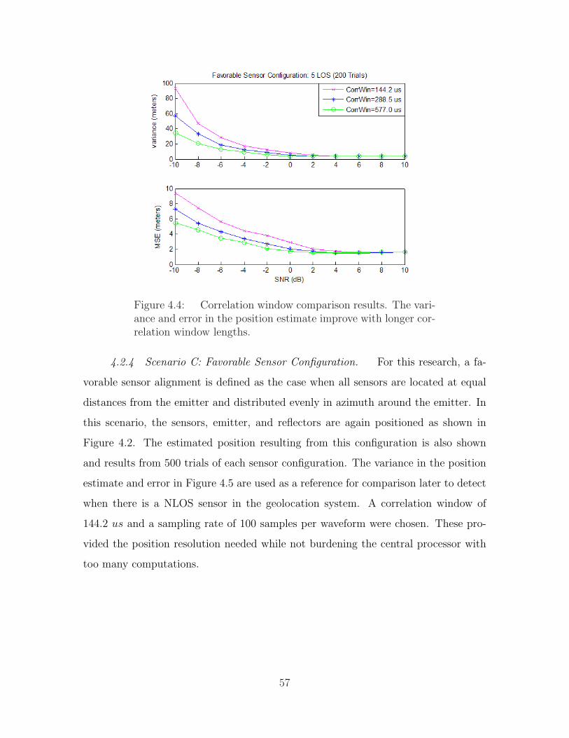
Figure 4.4: Correlation window comparison results. The vari-ance and error in the position estimate improve with longer cor-relation window lengths.

4.2.4 Scenario C: Favorable Sensor Configuration. For this research, a fa-

vorable sensor alignment is defined as the case when all sensors are located at equal

distances from the emitter and distributed evenly in azimuth around the emitter. In

this scenario, the sensors, emitter, and reflectors are again positioned as shown in

Figure 4.2. The estimated position resulting from this configuration is also shown

and results from 500 trials of each sensor configuration. The variance in the position

estimate and error in Figure 4.5 are used as a reference for comparison later to detect

when there is a NLOS sensor in the geolocation system. A correlation window of

144.2 us and a sampling rate of 100 samples per waveform were chosen. These pro-

vided the position resolution needed while not burdening the central processor with

too many computations.

57

Figure 4.5: Favorable LOS configuration data. The varianceand error is minimal while in this configuration.

4.2.5 Scenario D: NLOS Sensor Configuration. In this scenario, reflectors

are added to the favorable sensor configuration of Scenario C to simulate buildings

and towers that may block the emitter LOS path to a sensor. This configuration is

shown in Figure 4.6. The resulting position errors and variance in this configuration

at different SNR values are shown in Figure 4.7.

4.2.5.1 Detection and Mitigation of NLOS Sensor. The results in

Figure 4.7 show that when a NLOS sensor is included in the geolocation system, the

variance and error in the estimated position are much higher than when all sensors

have a LOS to the emitter. This result shows that position estimate variance can

provide an indication if there is a NLOS sensor present in the system. The geolocation

system uses this higher variance to detect when there is a NLOS sensor.

58

Figure 4.6: NLOS sensor configurations used in simulation.There are 4 LOS and 1 NLOS sensors. The estimated emit-ter position’s error is a result of all sensors TDOA informa-tion (including the NLOS sensor) included and used by the cen-tral processor to estimate the position of the low-power emitter(SNR = 0 dB).

Figure 4.7: NLOS configuration data. This figure shows howlarge the variance and error of the estimated position are whenthere is a NLOS sensor included in the position estimate.

59

4.2.5.2 Optimized Position Estimation in NLOS Configuration. Be-

cause the variance in Figure 4.7 is above the desired threshold for both cases of NLOS

sensor configurations, the geolocation system determines that there is a sensor with a

NLOS component. The sensor error detection and identification algorithm is then run

before the central processor estimates the final position. This algorithm calculates

the residual error in each sensor’s respective position estimates. These residuals are

ranked, and the sensor with the largest residual error is removed from subsequent

position estimate calculations. After the position is re-calculated with the remain-

ing sensor data, the resultant position estimate variance falls below the threshold

allowed, causing the estimated position error to also be much lower. This confirmed

that if there is just one NLOS sensor, the sensor with the highest residual variance

is the NLOS sensor. The case when the sensor with the highest residual variance is

not the sensor contributing the most variance in the position estimate is explored in

Section 4.2.6. The results after detecting and removing the NLOS sensor from the

geolocation system are shown in Figure 4.8. These results are consistent with baseline

results presented in Figure 4.5

60

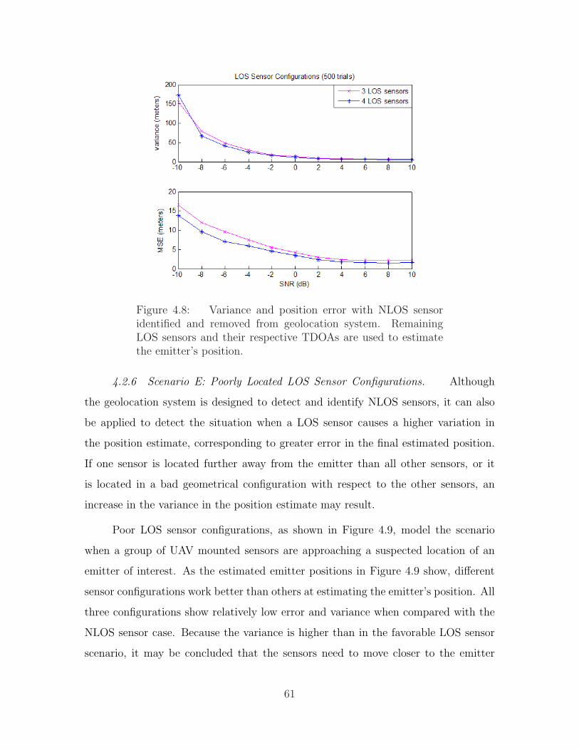
Figure 4.8: Variance and position error with NLOS sensoridentified and removed from geolocation system. RemainingLOS sensors and their respective TDOAs are used to estimatethe emitter’s position.

4.2.6 Scenario E: Poorly Located LOS Sensor Configurations. Although

the geolocation system is designed to detect and identify NLOS sensors, it can also

be applied to detect the situation when a LOS sensor causes a higher variation in

the position estimate, corresponding to greater error in the final estimated position.

If one sensor is located further away from the emitter than all other sensors, or it

is located in a bad geometrical configuration with respect to the other sensors, an

increase in the variance in the position estimate may result.

Poor LOS sensor configurations, as shown in Figure 4.9, model the scenario

when a group of UAV mounted sensors are approaching a suspected location of an

emitter of interest. As the estimated emitter positions in Figure 4.9 show, different

sensor configurations work better than others at estimating the emitter’s position. All

three configurations show relatively low error and variance when compared with the

NLOS sensor case. Because the variance is higher than in the favorable LOS sensor

scenario, it may be concluded that the sensors need to move closer to the emitter

61

to achieve similar variance in the position estimate and lower error in the estimated

position. Figure 4.10 shows the error and variances corresponding to the poor LOS

case plots.

Figure 4.9: Poor LOS sensor configurations used in simula-tion. The estimated emitter position error is a result of allsensor TDOA information being included and used by the cen-tral processor to estimate the position of the low-power emitter(SNR = 0 dB).

62

Figure 4.10: Poor LOS configuration data. This figure showsthe variance and error of the estimated position when the sensorsare located to one side of the emitter.

4.2.6.1 Detection and Mitigation of Poorly Located Sensors. In Fig-

ure 4.11, the resultant position error and respective variance is quite a bit larger than

is observed in Figure 4.9. The sensors, located almost in a zig-zag pattern, make it

more difficult for an estimator to converge to a position estimate. This is consistent

with the location error ellipses developed by [8] and discussed in Chapter II.

The results in Figure 4.12 show that even when all sensors have a LOS propa-

gation path to the emitter, there is considerable error and variance in the estimated

position of the emitter. The results also show how the variance of the position estimate

can indicate the existence of a poorly located LOS sensor.

63

Figure 4.11: Poor LOS sensor configuration. The estimatedemitter position error is a result of all sensors TDOA informationbeing included and used by the central processor to estimate theposition of the low-power emitter (SNR = 0 dB).

4.2.6.2 Position Estimate with Poorly Located Sensor Removed. Be-

cause the variance of the position estimate in Figure 4.12 is observed to be above

the desired variance of the favorable LOS case, the geolocation system detects that

there is a poorly located LOS sensor, so the sensor error detection and identification

algorithm is run before estimating the final position of the emitter. The residual

error in each sensor’s respective position estimates is calculated. These residuals are

ranked, and the sensor with the largest residual error is removed from the geolocation

system’s calculations. After the position is re-calculated with the remaining sensor

data, the resultant position estimate variance is compared with the variance of the

favorable LOS configuration. Several sensors are removed this way, then placed back

into the geolocation system before a sensor is determined to contribute the greatest

variance to the position estimate. This occurred because the sensor that caused the

most variance in the final position estimate does not have the highest residual. This

shows that the LOS sensor having the highest residual error is not necessarily the

64

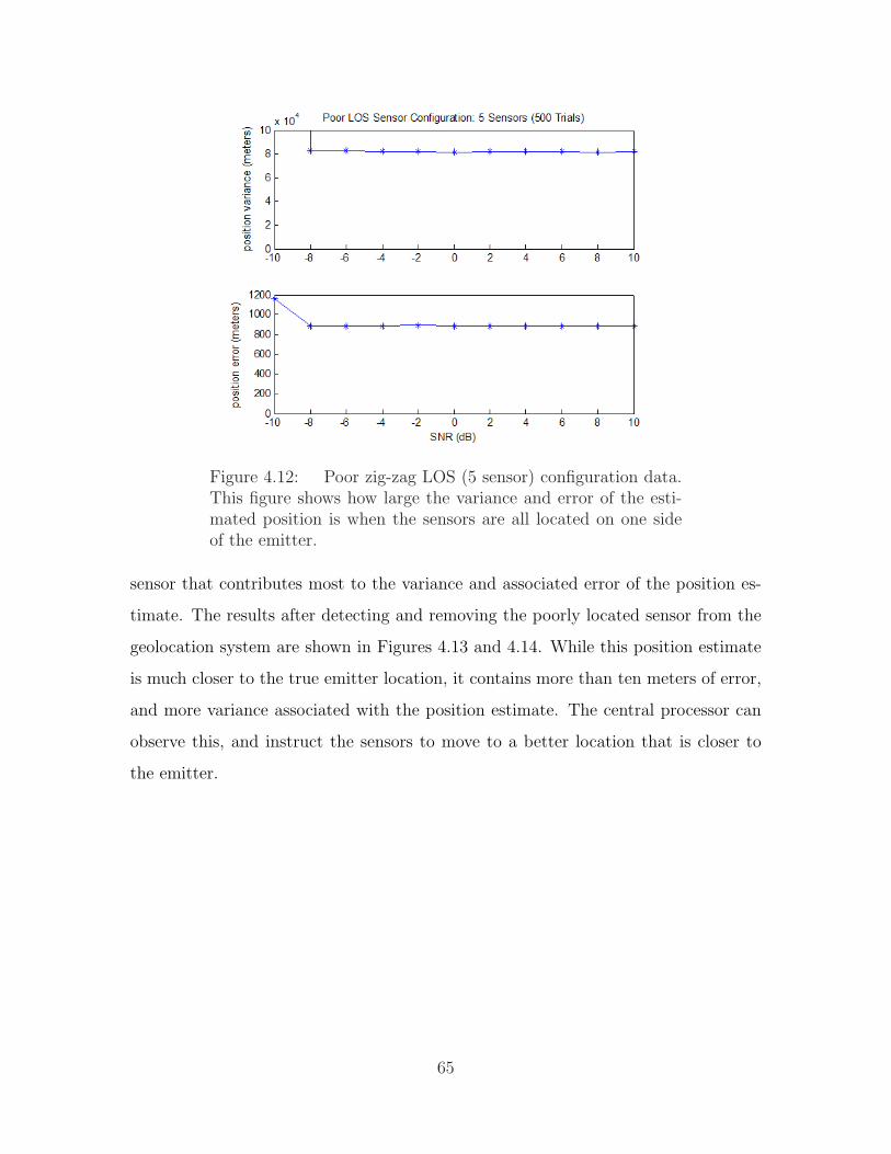
Figure 4.12: Poor zig-zag LOS (5 sensor) configuration data.This figure shows how large the variance and error of the esti-mated position is when the sensors are all located on one sideof the emitter.

sensor that contributes most to the variance and associated error of the position es-

timate. The results after detecting and removing the poorly located sensor from the

geolocation system are shown in Figures 4.13 and 4.14. While this position estimate

is much closer to the true emitter location, it contains more than ten meters of error,

and more variance associated with the position estimate. The central processor can

observe this, and instruct the sensors to move to a better location that is closer to

the emitter.

65

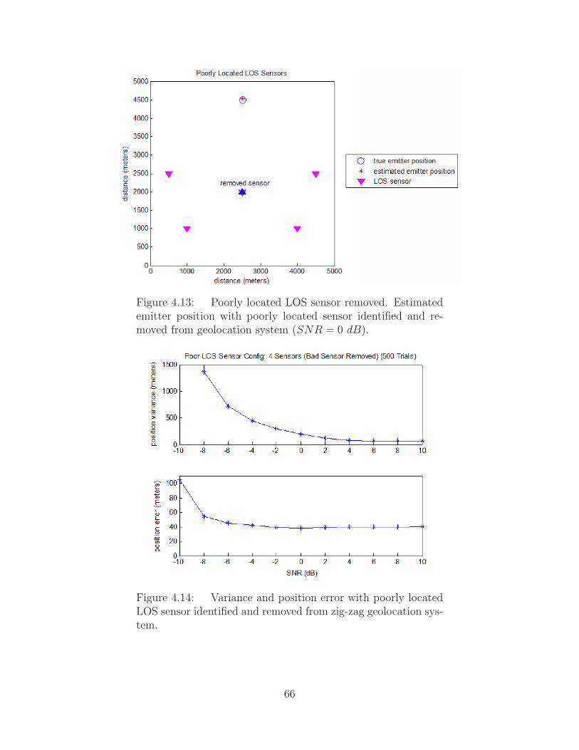
Figure 4.13: Poorly located LOS sensor removed. Estimatedemitter position with poorly located sensor identified and re-moved from geolocation system (SNR = 0 dB).

Figure 4.14: Variance and position error with poorly locatedLOS sensor identified and removed from zig-zag geolocation sys-tem.

66

4.3 Other Signal Results

Baseline results were obtained using a generated BPSK signal. While no other

signal types were used to test the geolocation system, autocorrelations shown in Fig-

ure 4.15 suggest similar results can be obtained with a GSM signal.

Figure 4.15: Autocorrelations of BPSK and GSM signals.These plots suggest that similar results can be optained witha GSM signal.

4.4 Summary

Based on simulation results, the ability to locate an emitter in an urban envi-

ronment was demonstrated. This chapter explored the effects different sensor con-

figurations and NLOS sensors have on the variance and accuracy of the estimated

emitter position. The system was able to identify and mitigate NLOS error and poor

sensor configurations using sensor residual variance.

In general, as the SNR increased the MSE of the position estimates decreased.

When the SNR dropped below −8 dB, significant error and variance occurred in the

position estimates. By averaging across a number of Monte Carlo trials over a specified

range of SNR values, a baseline containing the expected variance and position error

with various number of sensors and configurations was achieved for the geolocation

system.

67

The results presented are comparable with research completed at the Naval

Post Graduate school by Mantis [17] and the ongoing work of Hippenstiel [14]. While

their research goals were different, both used the TDOA method as a basis in the

development of their respective geolocation systems.

Chapter V provides conclusions of this research and recommendations for future

research.

68

V. Conclusions and Future Work Recommendations

5.1 Summary

This research presented the modeling methodology and results of a simulated

passive low-power emitter geolocation system. These simulation results and analysis

provide important insight that must be considered in the design and possible deploy-

ment of a geolocation system. Based on the results, a more robust geolocation system

that can detect and identify the presence of NLOS signals impinging upon poorly

located sensors, which add significant difficulty in passively locating emitters in the

urban environment, is possible.

5.2 Conclusions

It cannot be assumed that an arbitrary emitter can be located with an arbitrary

sensor configuration. If there is a very poor sensor configuration, the emitter position

estimate may be very far away from the true emitter’s location. In this situation,

the geolocation system’s estimated emitter location is incorrect with respect to range,

but can provide the direction the emitter is in. This allows the system to direct the

sensors closest to the emitter to obtain a better position estimate.

If the sensors are positioned around the emitter of interest, and there are at

least three sensors with a LOS path from the emitter, the accuracy of the geolocation

system and its ability to detect and mitigate a NLOS sensor was very good. In the

case where all sensors are located on one side of the emitter, the best location estimate

was found if the sensors were positioned in a semicircle facing the emitter. While not

a favorable sensor configuration, this did yield more accurate position estimates than

in the case when the sensors were aligned in a rough line perpendicular to the actual

emitter location.

69

5.3 Recommendations for Future Work

While the simulated TDOA geolocation system demonstrated its ability to lo-

cate an emitter through detection and mitigation of NLOS sensors, there are still

areas that could be expanded to make the system more robust. To implement the

system onto a UAV or UGV, more research needs to be completed.

Several different configurations were modeled and tested with the geolocation

system, but there are many more that could provide a more realistic scenario should

this be implemented onto a UAV or UGV system. This will make the system more

adaptable to the always changing sensor configurations.

Other types of low-power signals that are commonly used for command and

control, networking, and IED detonation (garage door openers, walkie talkies, etc.)

could be simulated using this geolocation system. By finding the variance and error

of the resultant position estimates, it could be determined how close the sensors need

to be to these types of emitters to be able to locate them with the required accuracy.

This research effort focused on the geolocation system, assuming all the com-

munications links between the sensors and central processor were properly working.

Cross-sensor communication is a key part of the system. Requirements for the central

processor need to be defined, including data links, bandwidth needed, and what kind

of connections will work. The determination of what geolocation tasks are assigned

to whom also needs to be determined. Some of the data processing, like correlating

signals, might be done at the sensors. This could minimize the amount of data they

have to send to the central processor.

While a range of SNR values were used in simulating geolocation system per-

formance, the effects of signal power loss due to propagation needs to be explored.

70

Appendix A. Matlab Code

Listing A.1: (appendix1/GeoSystem.m)%----------------------------------------------------------------% Passive Geolocation System ( GeoSystem.m)% Main program for passive geolocation system model.% Written by Myrna Montminy

5 %----------------------------------------------------------------

clear all; clc;

%----------------------------------------------------------------10 % Simulation Input Parameters

c = 3.00 e008; % speed of light (m/s)esym = 1.0e -009; % energy per output symboltsym = 3.7e -006; % symbol duration (s)

15 fnot = 1/ tsym; % number of symbols (bps)fc = 1; % carrier frequency (MHz)sigamp = sqrt (2* esym/tsym);nsamp = 100; % # of output waveform samples per

% symbol period20 fs = tsym/nsamp ; % number of samples/second

signal = ’BPSK’; % waveform used for simulation% signal = ’GMSK ’; % BPSK = baseline , GMSK = testRxTr = ’good’; % geometric layout of sensors

25 %RxTr = ’baad ’; % good is surrounding emitter% baad is all on one side of% emitter

numRx = 5; % number of sensorsranges = [5000 5000]; % sensor configuration range

30 axis_lim = [0 ranges (1) 0 ranges (2)];[Rx , Tr , reflec ] = RxTrConfig(RxTr , numRx , ranges);Rx_NLOS = [1 1 1 1 1 1]; % defines LOS (1) or NLOS (0)SNR = [ -10 -8 -6 -4 -2 0 2 4 6 8 10];M = length(SNR);

35 numtrials = 500;%----------------------------------------------------------------

%------------for v = 1:M, % loop running through SNR values

40 %------------

%------------for s = 1: numtrials , % loop running through trials%------------

45clear timvec ; clear sigvec ; clear max; clear Rx_nlos;

%--------------------------------------------------------if signal == ’GMSK’ % generates GSM signal

50 [timvec , sigvec ] = GsmSig(1,tsym ,fc,fs);

71

sigvec = sigvec * sigamp;

elseif signal == ’BPSK’ % generates BPSK signaldatsel = ’rand’; % select random data for BPSK sig

55 rbits = 148; % # of bits in one GSM sig burstndelay = 0; % # of leading samples preceeding

% first valid sample[timvec ,sigvec ] = BpskSig(datsel ,rbits ,ndelay ,...

fnot ,SNR(v),tsym ,esym ,nsamp ,0);60 else

signal = signalend

%--------------------------------------------------------65 % sample rate information

ts = timvec (2) - timvec (1);fs = 1/ ts;CorWin = 0.577e -003/4; % length of corr window (s)N = floor(CorWin/ts); % length of corr window (# samp)

70 tau = (-N+1:N-1) ’*ts;

% plot of original signal and its correlation% figure ; hold on;% subplot (2,1,1);

75 % plot(timvec (1:N),sigvec (1:N));% PlotDetails(’BPSK Signal - no noise ’,’time (s) ’,...% ’amplitude (v) ’,0,0,1,0);

timvec = timvec (1:N);80 s1 = VecShift(sigvec ,0);

s1 = s1(1:N);sigvec (1:N) = s1;sigvec = sigvec ’;

85 % subplot (2,1,2)% figure;% ww = smooth(abs(xcorr(s1 ,s1)) ,8);% ww = ww/max(ww);% plot(tau , ww);

90 % axis ([-2.0e -004 2.0e -004 0 1])% plot_details(’Sampling Frequency = 2.70 MHz ...% (CorrWin = 144.2 us)’,’time (s)’,’magnitude ’,0,0,0,0);

%--------------------------------------------------------95 % calculate true arrival time delays in received signals

for i = 1: numRx ,if Rx_NLOS(i) == 0,

D(i) = ArrTime(Tr , Rx(i,:) , c, reflec(i,:));else

100 D(i) = ArrTime(Tr , Rx(i,:) , c);endDs(i) = D(i) * fs;

72

sigvec_new (:,i) = VecShift(sigvec ,Ds(i));sigvec_fnl (1:N,i) = sigvec_new (1:N,i);

105 endsigvec = sigvec_fnl;clear sigvec_fnl ; clear sigvec_new;

%--------------------------------------------------------110 % generate noise

snrat = 10^( SNR(v)/10); % calc ratio of SNRsigamp = sqrt (2* esym/tsym); % signal amplitudenosamp = sqrt(esym/(tsym*snrat)); % noise amplitude

115 for k = 1: numRx ,noise_new(:,k) = nosamp .* randn(size(sigvec(:,k)));sigvec(:,k) = sigvec(:,k) + noise_new(:,k);

end

120 %--------------------------------------------------------% compute cross correlation , smooth , find peak valueTDOA_est = TdoaEst(sigvec , Rx , tau);

%--------------------------------------------------------125 % estimate emitter position , calc residual variance wrt

% each receiver ’s position estimatesfor m = 1: numRx ,

[LocEst(m,:) , LocVar(m,:) , PosHis ] = ...PosEstimator(Rx , m, Tr , c, ( TDOA_est(m,:)));

130 residual(m) = mean(LocVar(m,:));if residual(m) > 200, % detect if sensor has NLOS

multipath = 1;else

multipath = 0;135 end

end

LocEstVar(s,:) = var(LocEst ,1);PosEstVar(s) = mean(LocEstVar(s,:));

140%--------------------------------------------------------% take out each Rx seperately to see if estimated% position convergesif multipath > 0,

145 clear LocEst;[Rx_multipath , RxNLOS , LocEst ] = ...

FindNlosRx(multipath ,Tr ,Rx ,Rx_NLOS ,reflec ,c);else

multipath = multipath;150 end

%--------------------------------------------------------% final estimated location at specified SNR valueif length(LocEstFix) > 2,

73

155 location = mean(LocEst);else

location = LocEst;end

160 Pos(s,:) = location;PosErr(s) = (( Tr(1)-Pos(s,1))^2 + ...

(Tr(2)-Pos(s,2))^2 ) ^(1/2);

%------------165 end % end of trial runs loop s

%------------

PosVar(v,:) = var(Pos ,1);% variance wrt each trial position average

170 PosVar(v) = mean(PosVar(v,:));% variance wrt each trial variance average relative to% each Rx ’s position estimate

PosVarRes(v) = mean(mean_var);PosEstVarRx(v) = mean(PosEstVar);

175 % variance wrt each Rx ’s position estimate variancePosAve(v,:) = mean(Pos);

% estimated position average over s trialsPos2Err(v) = mean(PosErr);

% average estimated position error over s trials180

%------------end % end of main process loop v%------------

185 %----------------------------------------------------------------% plotting SNR versus position variance

close all;

190 figure;subplot (211);hold on;plot(SNR ,PosEstVarRx , ’*-’);PlotDetails(’Sensor Configuration : 5 LOS (500 Trials)’ ,...

195 0,’position variance ( meters)’ ,0,0,0,1);% line(xlim ,[max(ylim) max(ylim)],’color ’,’k’);% line([max(xlim) max(xlim)],ylim ,’color ’,’k’);

%----------------------------------------------------------------200 % plotting SNR vs position error

subplot (212);hold on;plot(SNR ,Pos2Err ,’*-’);

205 PlotDetails (0,’SNR (dB)’ ,...’position error ( meters)’ ,0,0,0,1);

74

% line(xlim ,[max(ylim) max(ylim)],’color ’,’k’);% line([max(xlim) max(xlim)],ylim ,’color ’,’k’);

210 %----------------------------------------------------------------% plotting sensors with estimated positions for each SNR valuefigure ; hold on;%[Rx , Tr , reflec ] = rx_locations(RxTr , 5, ranges);PlotRxTr(Rx , Tr , ranges);

215 %plot(Rx(3,1),Rx(3,2) , ’b^’, ’markersize ’, 10);for xx = 1:M,

plot(PosAve(xx ,1),PosAve(xx ,2),’+’);end% line(xlim ,[max(ylim) max(ylim)],’color ’,’k’);

220 % line([max(xlim) max(xlim)],ylim ,’color ’,’k’);

% save GSM_500_LOS_3good_5wls Pos* Rx Tr;

75

Listing A.2: (appendix1/RxTrConfig.m)

function [Rxy , Tr , reflec ] = RxTrConfig(RxTr , numRx , ranges)

%----------------------------------------------------------------5 % This function sets sensor , transmitter and reflector locations

% Written by Myrna Montminy%% In: RxTr = ’good ’ or ’baad ’% numRx = number of receivers

10 % ranges = area receivers can be in (i.e. 5000 , 5000)%% Out: Rx = matrix of receiver lcoations within range% Tr = emitter location% reflec = reflector locations

15 %----------------------------------------------------------------

if RxTr == ’good’;Tr = [2500 2500];if numRx == 3,

20 Rxy(1,:) = [2500 4500];Rxy(2,:) = [4500 500];Rxy(3,:) = [500 500];reflec = [3500 4000; 3500 500; 1500 500];

elseif numRx == 4,25 Rxy(1,:) = [4000 4000];

Rxy(2,:) = [4000 1000];Rxy(3,:) = [1000 1000];Rxy(4,:) = [1000 4000];reflec = [4000 3000; 4000 2000; 1000 2000; 1000 3000];

30 elseif numRx == 5,Rxy(1,:) = [2500 4500];Rxy(2,:) = [4500 3000];Rxy(3,:) = [4000 500];Rxy(4,:) = [1000 500];

35 Rxy(5,:) = [500 3000];reflec = [3500 4000; 4000 2000; 4000 2000; 1000 2000;...

1000 2000];elseif numRx == 6,

Rxy(1,:) = [3500 4500];40 Rxy(2,:) = [4500 2500];

Rxy(3,:) = [3500 500];Rxy(4,:) = [1500 500];Rxy(5,:) = [500 2500];Rxy(6,:) = [1500 4500];

45 reflec = [4500 2500; 3500 500; 1500 500; 500 2500;...1500 4500; 3500 4500];

elsenumRx = numRx

end50

elseif RxTr == ’baad’,

76

Tr = [2500 4500];if numRx == 3,

Rxy(1,:) = [3500 1500];55 Rxy(2,:) = [2500 500];

Rxy(3,:) = [1500 1500];reflec = [3500 4000; 3500 500; 1500 500];

elseif numRx == 4,Rxy(1,:) = [4000 2000];

60 Rxy(2,:) = [3000 500];Rxy(3,:) = [2000 500];Rxy(4,:) = [1000 2000];reflec = [3500 4000; 3500 500; 1500 500];

elseif numRx == 5,65 Rxy(1,:) = [4500 2500];

Rxy(2,:) = [4000 1000];Rxy(3,:) = [2500 500];Rxy(4,:) = [1000 1000];Rxy(5,:) = [500 2500];

70 reflec = [4500 4000; 4000 4000; 3500 1000; 1000 4000;...500 4000];

elsenumRx = numRx

end75

elseif RxTr == ’rand’,for i = 1: numRx ,

Rxy(i,:) = [ floor(rand*ranges (1))+trans (1) ; ...floor(rand*ranges (2))+trans (2)];

80 end

% pick Tr located within Rx rangesRx_range = range(Rxy);Tr = [( floor(rand*Rx_range (1))+min(Rxy(:,1))) ...

85 (floor(rand*Rx_range (2))+min(Rxy(:,2)))];

elseRxTr = RxTr

end90

return;

77

Listing A.3: (appendix1/GsmSig.m)

function[GMSK_time , GMSK_sig_out , pulse1 ] = ...GsmSig(num_frames ,Ts,fc,fs);

5 %----------------------------------------------------------------% This function generates a GMSK waveform signal% Adopted from a script created by Clint Sikes%% In: num_frames = 1 frame_num = 0.2354s or 51 TDMA frames

10 % Ts = signal length (us)% fc = carrier frequency% fs = signal frequency%% Out: GMSK_time = time vector for GSM signal

15 % GMSK_sig_out = simulated GSM signal with no noise% pulse1 = one pulse length of signal (577 us)%----------------------------------------------------------------

pulselength = 577; % Length of pulse (us)20 L = 3.7; % Length of GMSK Pulse Shape (us)

ns = fs*Ts; % Number of samples/bit (4)BT = 0.3; % BT Parameter of GMSK Pulseh = 0.5; % Modulation Index of GMSK Pulsez0 = 0; % Initial Phase of GMSK Signal

25 N = floor(pulselength/L); % Number of bits in T1%N = 192;

%----------------------------------------------------------------% generate GMSK pulse shape

30 % Ts = 3.7;tpulse = [ -1.5*Ts:1/fs:1.5*Ts -1/fs];g = 1/(2* Ts).*( qfunc (2*pi*BT.*(tpulse -Ts/2) ./...

(Ts*sqrt(log (2))))-qfunc (2*pi*BT.*( tpulse+Ts/2) ./...(Ts*sqrt(log (2)))));

35 g = g/(2* sum(g));

%----------------------------------------------------------------% uncomment when outputing GSM signal > 1 pulse length% seg = [1 2 3];

40 % frame_len = floor(num_frames /3);% frames = [];% for m = 1: frame_len ,% frames = [ frames seg];% end

45GSM_sig = [];% for k = 1: length(frames),

% Generate 4 pulses to simulate50 pulse4 = [];

for j = 1:4 ,

78

clear sGMSK;clear bits;% generate 1 pulse one time slot (TS) long (15/26 ms)

55 % generate vector of binary bitsbitsin=round(rand(1,N)) ’;% Converting bits to NRZfor i=1:N

if bitsin(i)==060 bits(i)=-1;

elsebits(i)=1;

endend

65 bits=bits ’;% generate SOI[Phase ,sGMSK ]= GmskMod(L,bits ,ns,fc,Ts,N,BT,g,h);pulse = sGMSK;% TDMA = 8 time slots

70 zero_vec = zeros (1,7* length(sGMSK));pulse4 = [ pulse4 pulse zero_vec ];

% time_p4 = time_p4 + 8;pulse1(j,:) = pulse;

end75 time4 = linspace (0 ,0.000577*8*4 , length(pulse4));

%----------------------------------------------------------------% uncomment when outputing GSM signal > 1 pulse length% % implement typical spacing while phone is active

80 % % time_len = 0;% if frames(k) == 1,% zero_vec1 = nosamp .* randn (1,15* length(pulse4));% GSM_sig = [ GSM_sig new_noisy_GMSK zero_vec1 ];% % time_len = time_len + (16* time_p4);

85 % elseif frames(k) == 2 ,% zero_vec2 = nosamp .* randn (1,34* length(pulse4));% GSM_sig = [ GSM_sig new_noisy_GMSK zero_vec2 ];% % time_len = time_len + (35* time_p4);% else ,

90 % zero_vec3 = nosamp .* randn (1,50* length(pulse4));% GSM_sig = [ GSM_sig new_noisy_GMSK zero_vec3 ];% % time_len = time_len + (51* time_p4);% end

95 % implement typical spacing while phone is active% time_len = 0;% if frames(k) == 1,% zero_vec1 = zeros (1,15* length(pulse4));% GSM_sig = [ GSM_sig pulse4 zero_vec1 ];

100 % % time_len = time_len + (16* time_p4);% elseif frames(k) == 2 ,% zero_vec2 = zeros (1,34* length(pulse4));% GSM_sig = [ GSM_sig pulse4 zero_vec2 ];

79

% % time_len = time_len + (35* time_p4);105 % else ,

% zero_vec3 = zeros (1,50* length(pulse4));% GSM_sig = [ GSM_sig pulse4 zero_vec3 ];% % time_len = time_len + (51* time_p4);% end

110 %%% end

% time_len = time_len * 0.000577;115 time_len = num_frames * 51 * 8 * 0.000577;

% time = linspace (0 ,(0.000570*4*8*51*6) ,length(GSM_sig));time = linspace(0,time_len ,length(GSM_sig));

% data is large - reshape to output to main file120 % GMSK_sig_out = reshape(GSM_sig , length(GSM_sig)/...

% length(pulse4) , (length(pulse4)));% GMSK_time = reshape(time , length(time)/length(pulse4) , ...% (length(pulse4)));

125 GMSK_sig_out = pulse4;GMSK_time = time4;

return;

80

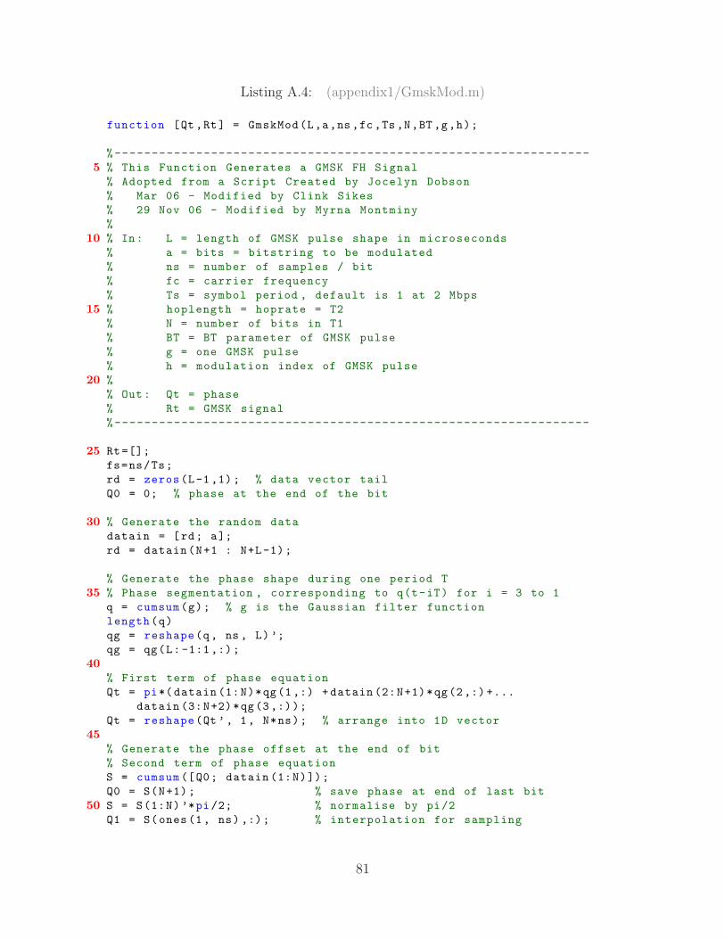
Listing A.4: (appendix1/GmskMod.m)

function [Qt ,Rt] = GmskMod(L,a,ns ,fc ,Ts ,N,BT ,g,h);

%----------------------------------------------------------------5 % This Function Generates a GMSK FH Signal

% Adopted from a Script Created by Jocelyn Dobson% Mar 06 - Modified by Clink Sikes% 29 Nov 06 - Modified by Myrna Montminy%

10 % In: L = length of GMSK pulse shape in microseconds% a = bits = bitstring to be modulated% ns = number of samples / bit% fc = carrier frequency% Ts = symbol period , default is 1 at 2 Mbps

15 % hoplength = hoprate = T2% N = number of bits in T1% BT = BT parameter of GMSK pulse% g = one GMSK pulse% h = modulation index of GMSK pulse

20 %% Out: Qt = phase% Rt = GMSK signal%----------------------------------------------------------------

25 Rt=[];fs=ns/Ts;rd = zeros(L-1,1); % data vector tailQ0 = 0; % phase at the end of the bit

30 % Generate the random datadatain = [rd; a];rd = datain(N+1 : N+L-1);

% Generate the phase shape during one period T35 % Phase segmentation , corresponding to q(t-iT) for i = 3 to 1

q = cumsum(g); % g is the Gaussian filter functionlength(q)qg = reshape(q, ns , L) ’;qg = qg(L:-1:1,:);

40% First term of phase equationQt = pi*( datain (1:N)*qg(1,:) + datain (2:N+1)*qg(2,:) +...

datain (3:N+2)*qg(3,:));Qt = reshape(Qt ’, 1, N*ns); % arrange into 1D vector

45% Generate the phase offset at the end of bit% Second term of phase equationS = cumsum ([Q0; datain (1:N)]);Q0 = S(N+1); % save phase at end of last bit

50 S = S(1:N) ’*pi/2; % normalise by pi/2Q1 = S(ones(1, ns) ,:); % interpolation for sampling

81

Q1 = Q1(:) ’;% Combine to give the final phaseQt = (Qt + Q1).*(h/(1/2)); %Normalize by modulation Index "h"

55for i=1:N

% Form signal to be transmittedn = [(i-1)*Ts:1/fs:i*Ts -1/fs]; % form time baseI = cos (2*pi*fc*n).*cos(Qt(fs*Ts*(i-1)+1:fs*Ts*i));

60 % in -phase componentQ = sin (2*pi*fc*n).*sin(Qt(fs*Ts*(i-1)+1:fs*Ts*i));

% quadrature componentRt_temp = I - Q; % transmitted signalRt=[Rt Rt_temp ];

65 end

return;

82

Listing A.5: (appendix1/BpskSig.m)

function [time ,sigvec ] = BpskSig(datsel ,rbits ,ndelay ,fnot ,...snr ,tsym ,esym ,nsamp ,noisamp)

5 %----------------------------------------------------------------% This function produces a sampled MPSK output waveform with% symbols generated per Eq 4.31 of Sklar ’s Digital% Communications text (2nd Ed.)%% [1] = > s1 => Phz = 180 Deg

10 % [0] = > s2 => Phz = 0 Deg% BPSK_MOD Function : Binary Phase Shift Keying Modulator%----------------------------------------------------------------%% Developed : Apr 04

15 % Dr. Michael A. Temple% Modified by Capt Montminy , Dec 2006%% In:% datsel - Data control variable:

20 % ’user ’ --> User SUPPLIED Data (" indata ") for Modulation% ’rand ’ --> Random Data GENERATED for Modulation% rbits - For " datsel " = ’rand ’ ... Number of " rbits"% Randomly generated for Modulation% ndelay - Number of LEADING samples preceeding first valid

25 % sample of first Complete Symbol% fnot - Modulator Output Frequency ( Hertz)% snr - Input Signal -to -Noise Ratio in Decibels (dB)% tsym - SYMbol Time / Duration% esym - Energy per putput SYMbol

30 % nsamp - Number of output waveform SAMPles per Symbol% Period (tsym)% noisamp - amplitude of noise wrt signal amplitude%% Out:

35 % time - sample time vector% sigvec - modulated signal vector%----------------------------------------------------------------

msym = 2; % sets default to BPSK (M=2)40 wnot = 2* pi*fnot; % radian frequency of carrier

snrat = 10^( snr /10); % calculate tatio form of input SNRsigamp = sqrt (2* esym/tsym); % signal component amplitudenosamp = sqrt(esym/( snrat*tsym)); % amplitude of received

% noise term45

% initial SYNChronization BIT vector ( syncbit)syncbit = [1,1,1,0,0,0,1,0,0,1,0]; % 11-Bit " Barker Sequence"

% IF datsel = " user" use " indata " vector as " rdata " vector50 rdata = []; % Initialize Data Vector

if datsel ==’user’

83

rdata = indata;rdata = cat(2,syncbit ,rdata);rbits = length(rdata);

55 rbits = rbits - mod(rbits ,2);end

% IF datsel = " rand" generate a Random " rdata " vector of length% "rbits"

60 if datsel ==’rand’rbits = rbits - mod(rbits ,2);for jbits = 1: rbits % (rbits -4)

y = rand;if(y<0.5)

65 rdata(jbits) = 1;else

rdata(jbits) = 0;end

end70 rbits = length(rdata);

endbitsin = rdata ; % actual BITS INto the Modulator

% calculate number of symbol periods (nsym) in RDATA75 bitsym = 1; % number of bits/symbol = 1 for BPSK

nsym = round(rbits/bitsym);tstep = tsym/nsamp;modout = [];

80 % Initialize " Sampled " Continuous Waveform vector ( sigvec) and% total Time vector (time)with leading zero samples

% Assign initial " LEADING " waveform sample and time valuessigvec = [];

85 %sigvec = zeros(1,ndelay);time = [];tlow = -tstep*ndelay;thgh = tstep *(nsym*nsamp -1);time = [ tlow:tstep:thgh];

90 ntime = length(time); % total number of initial time valuesrandn(’state’,sum (100* clock)); % Reset Random # Generator

%----------------------------------------------------------------% Calculate Sampled Output Waveform over each " Symbol Interval"

95 %----------------------------------------------------------------

% Initialize Symbol TIMe INTerval ( timint) , 0 < t < Tsymtimint = [];tlow = 0;

100 thgh = tstep *(nsamp -1);timint = [ tlow:tstep:thgh];%for jsym = 1: bitsym:nsym*bitsym

84

% Note: jsym step size = BITSYM105 symbol = sigamp*cos(wnot*timint + pi*rdata(jsym));

% Symbol over symbol time ( timint)sigvec = [ sigvec ,symbol ];

% Create Composite " Sampled " Modulated Signal vectorend

110%----------------------------------------------------------------% End of main " Symbol Interval " Loop Calculations%----------------------------------------------------------------

115 % Fill " LEADING " samples of " sigvec " with last symbol dataif ndelay > 0

sigvec (1: ndelay)=sigvec (( length(sigvec)-ndelay +1) :...length(sigvec));

end120 % Generate and add zero mean AWGN vector over total signal

% interval.% Noise amplitude ( nosamp) is calculated using inputs : snr ,% esym , tsymif noisamp == 1,

125 noise = nosamp*randn(size(sigvec));else

noise = 0;endsigvec = sigvec + noise;

130 % TOC % Stop Subroutine Timerreturn

85

Listing A.6: (appendix1/PlotDetails.m)

function PlotDetails(titlestr , xlabelstr , ylabelstr , ...axis_lim , axis_specs , hold_specs , grid_specs)

5 %----------------------------------------------------------------% This function plots the details for a figure% Written by Myrna Montminy%% In: title = title (*)

10 % xlabel = xlabel (*)% ylabel = ylabel (*)% axis_lim = axis (*)% axis_apecs = square (1) , image (2) , both (12) , no specs (0)% hold = on(1) / off (0)

15 % grid_specs = on(1) / off (0)%% Out: details plotted on desired graph%----------------------------------------------------------------

20 if titlestr == 0,titlestr = titlestr;

elsetitle(titlestr);

end25 if xlabelstr == 0,

xlabelstr = xlabelstr;else

xlabel(xlabelstr);end

30 if ylabelstr == 0,ylabelstr = ylabelstr;

elseylabel(ylabelstr);

end35 if axis_lim == 0,

axis_lim = axis_lim;else

axis(axis_lim);end

40 if axis_specs == 1,axis square;

elseif axis_specs == 2,axis image;

elseif axis_specs == 12 ,45 axis image;

axis square;else

axis_specs = axis_specs;end

50 if hold_specs == 0,hold off;

86

elsehold on;

end55 if grid_specs == 1,

grid on;else

grid_specs = grid_specs;end

60return

Listing A.7: (appendix1/smooth.m)

function y = smooth(x,M)

%----------------------------------------------------------------5 % This function smoothes the input vector by taking the moving

% average over the amount specified% Written by Dr. Robert Mills , Jul 06%% In: x = Input vector

10 % M = smoothing factor (even)%% Out: Y = smoothed version of X%----------------------------------------------------------------

15 if M < 2y=x;

elseN=length(x); % get length of input vectors=ones(1,M+1)/(M+1);

20 y=conv(s,x);y=y( 1+M/2:N+M/2 );

endreturn

87

Listing A.8: (appendix1/ArrTime.m)

function [ sig_time ] = ArrTime(Tr , R1 , c, refl)

%----------------------------------------------------------------5 % This function calculates the true arrival time of the signal

% at each of the sensors% Written by Myrna Montminy%% In: Tr = transmitter location

10 % R1 = receiver location% refl = reflection location% c = speed of light in feet/sec%% Out: sig_time = arrival time of the signal

15 %%----------------------------------------------------------------

% distance between transmiter of interest and receiverD = ((( R1(2)-Tr(2))^2) +((R1(1)-Tr(1))^2))^0.5;

20% added propagation time due to a reflectionif nargin == 3 ,

D = D;else

25 % added propagation time from multipath errorsDx = ((( Tr(2)-refl (2))^2) +((Tr(1)-refl (1))^2))^0.5;

D = Dx + ((( R1(2)-refl (2))^2)+((R1(1)-refl (1))^2))^0.5;hold on;plot(refl (1),refl (2),’s’);

30 end

% propagation time of signal from transmitter to receiversig_time = D / c;

35 return;

88

Listing A.9: (appendix1/VecShift.m)

function [Y] = VecShift(X,d)

%----------------------------------------------------------------5 % This function shifts the input vector by the amount

% specified . Zeros are shifted in one end and data is lost% out the other (i.e., no circular shift). Input vector can be% row or column.% Written by Dr. Robert Mills , Jul 06

10 % Modified by Myrna Montminy , Oct 06%% In: X = Input vector% d = shift value ( >0 = shift right )%

15 % Out: Y = shifted version of X%----------------------------------------------------------------

Xrow = X(:) ’;N = length(Xrow);

20 N = 2*N;ad = abs(d);Zrow = zeros(1,ad);Zpad = zeros(1,N);

25 if d == 0Yrow = [ Xrow Zpad];

Y = Yrow (1:N);elseif d > 0

Yrow = [ Zrow Xrow Zpad];30 Y = Yrow (1:N);

elseif d < 0Yrow = [ Xrow Zrow];Yrow = Yrow( ad+1:ad+N );

end35

% return Y as either row or column depending on inputY = Y’;return

89

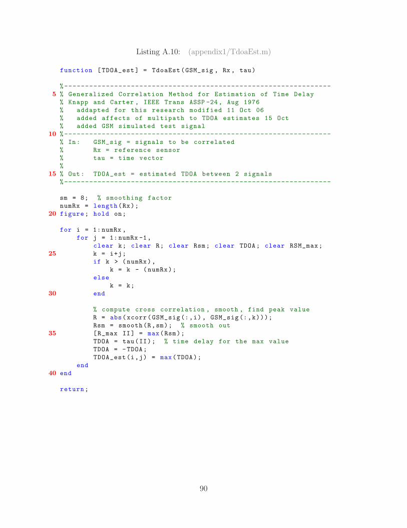
Listing A.10: (appendix1/TdoaEst.m)

function [ TDOA_est ] = TdoaEst(GSM_sig , Rx , tau)

%----------------------------------------------------------------5 % Generalized Correlation Method for Estimation of Time Delay

% Knapp and Carter , IEEE Trans ASSP -24, Aug 1976% addapted for this research modified 11 Oct 06% added affects of multipath to TDOA estimates 15 Oct% added GSM simulated test signal

10 %----------------------------------------------------------------% In: GSM_sig = signals to be correlated% Rx = reference sensor% tau = time vector%

15 % Out: TDOA_est = estimated TDOA between 2 signals%----------------------------------------------------------------

sm = 8; % smoothing factornumRx = length(Rx);

20 figure ; hold on;

for i = 1: numRx ,for j = 1: numRx -1,

clear k; clear R; clear Rsm; clear TDOA; clear RSM_max;25 k = i+j;

if k > ( numRx),k = k - (numRx);

elsek = k;

30 end

% compute cross correlation , smooth , find peak valueR = abs(xcorr(GSM_sig(:,i) , GSM_sig(:,k)));Rsm = smooth(R,sm); % smooth out

35 [R_max II] = max(Rsm);TDOA = tau(II); % time delay for the max valueTDOA = -TDOA;TDOA_est(i,j) = max(TDOA);

end40 end

return;

90

Listing A.11: (appendix1/FindNlosRx.m)

function [multipath , Rx_nlos , est_pos ] = ...FindNlosRx(multipath , Tr , Rx , Rx_NLOS , reflec , c)

5 %----------------------------------------------------------------% This function test the given sensor for NLOS by removing it% and re -estimating the position . This function continues% to be called until a NLOS sensor is identified and removed% and the variance is found below desired max.

10 % Written by Myrna Montminy%% In: multipath = 1 for 1 NLOS detected , 2 for 2 NLOS detected% Tr = transmitter location% Rx = 3 receiver locations

15 % Rx_NLOS = sensor being tested for NLOS% reflec = reflector% c = speed of light (m/s)%% Out: multipath = 0 for no NLOS detected

20 % Rx_nlos = sensor identified as NLOS% est_post = estimated location of emitter%----------------------------------------------------------------

numRx = length(Rx);25 % take out each Rx seperately to see if est pos converges

n = 1; % Rx1 thru every Rx until multipath Rx is found% if mult Rx is not found , assume 2 mult. Rx ’s exist

while multipath == 1 ,30 Rxx = circshift(Rx , ((n)*(-1)));

Rxx = Rxx (1:( numRx -1) , :);Rx_NLOSx = circshift(Rx_NLOS ’, ((n)*(-1)));Rx_NLOSx = Rx_NLOSx ’;Rx_NLOSx = Rx_NLOSx (1: ( numRx -1));

35 reflecX = circshift(reflec , (n*(-1)));reflecX = reflecX (1:( numRx -1) , :);[TDOA_true , TDOA_outX ] = TdoaEst(Tr , Rxx , c, ...

reflecX , Rx_NLOSx);[location_est , location_est_std ] = ...

40 PosEstimator(Rxx , 1, Tr , c, ( TDOA_outX (1,:)));if location_est_std (1) > 100,

multipath = 1;elseif location_est_std (2) > 100,

multipath = 1;45 else

multipath = 0;Rx_multipath = n;Rx_nlos_xx = 0;est_pos(n,:) = location_est;

50 endclear Rxx; clear Rx_NLOSx ; clear reflecX ; clear TDOA_outX;

91

n = n+1;if n > ( numRx +1),

multipath = 0; % !! need to change this back to 2 !!55 % after each Rx is pulled to test for multipath , if

% there is still large std in the estimated position ,% then there are 2 Rx’s with multipath

elsemultipath = multipath;

60 endend % end of 1 NLOS test while loop

p = 1;% 2 Rx ’s with NLOS:

65 while multipath == 2 ,Rx1 = circshift(Rx , ((p)*(-1)));Rx1 = Rx1 (1:( numRx -1) , :);Rx_NLOSx1 = ( circshift(Rx_NLOS ’, ((p)*(-1)))) ’;Rx_NLOSx1 = Rx_NLOSx1 (1: ( numRx -1));

70 reflecX1 = circshift(reflec , (p*(-1)));reflecX1 = reflecX1 (1:( numRx -1) , :);for i = 2: numRx ,

Rx2 = circshift(Rx1 , ((i-2)*(-1)));Rx2 = Rx2 (2:( numRx -1) , :);

75 Rx_NLOSx2 = ( circshift(Rx_NLOSx1 ’, ((i-2)*(-1)))) ’;Rx_NLOSx2 = Rx_NLOSx2 (2: ( numRx -1));reflecX2 = circshift(reflecX1 , ((i-2)*(-1)));reflecX2 = reflecX2 (2:( numRx -1) , :);[TDOA_true , TDOA_outX2 ] = TdoaEst(Tr , Rx2 , c, ...

80 reflecX2 , Rx_NLOSx2);[location_Rx2 , location_Rx2_std ] = ...

PosEstimator(Rx2 , 1, Tr , c , ...(TDOA_outX2 (1,:)));

if location_Rx2_std (1) > 100,85 multipath = 2;

elseif location_Rx2_std (2) > 100,multipath = 2;

elsemultipath = 0;

90 multipath_Rx (1,:) = pmultipath_Rx (2,:) = iest_pos2(i,:) = location_Rx2;

endclear Rx2; clear Rx_NLOSx2 ; clear reflecX2;

95 clear TDOA_outX2;endclear Rx1; clear Rx_NLOSx1 ; clear reflecX1;p = p+1;if p > ( numRx +1),

100 multipath = 3;% after each Rx is pulled to test for multipath , if% there is still large std in the estimated position ,% then there are 2 Rx’s with multipath

92

else105 multipath = multipath;

endend % end of 2 NLOS test while loop

return

93

Listing A.12: (appendix1/PosEstimator.m)

function [ location_est , location_Rx_var , LocHis ] = ...PosEstimator(Rx , Rx_num , Tr , c, TDOAs)

5 %----------------------------------------------------------------% This function uses the maximum likelihood method to estimate% the position from TDOA measurements . A different location% is estimated from each 3-wise combonation of TDOA% measurments inputed.

10 % Written by Myrna Montminy%% In: Rx = all receiver locations% matrix of all locations (up to 6 receiver locations)% Rx_num = Rx referenced for location estimation

15 % Tr = emitter location (true)% c = speed of light% TDOAs = TDOA between all receiver combinations% vector of specified Rx with all other Rx ’s (in time)%

20 % Out: location_est = estimated location of emitter% location_Rx_std = standard deviation of estimated location%----------------------------------------------------------------

numRx = length(Rx);25 Rxx = circshift(Rx ,(( Rx_num -1)*(-1)));

if numRx == 3,Rx1 = [ Rxx(1,:); Rxx(2,:); Rxx(3,:)]; % Rx 1 2 3TDOA1 = [ TDOAs (1); TDOAs (2)];

30 [location_est , LocHis ] = WlsEst(Rx1 , Tr , c, TDOA1);

elseif numRx == 4,% estimated location referenced to specified sensor , Rx_numRx1 = [ Rxx(1,:); Rxx(2,:); Rxx(3,:)]; % Rx 1 2 3

35 TDOA1 = [ TDOAs (1); TDOAs (2)];[location_est (1,:) , LocHis ] = WlsEst(Rx1 , Tr , c, TDOA1);

Rx2 = [ Rxx(1,:); Rxx(2,:); Rxx(4,:)]; % Rx 1 2 4TDOA2 = [ TDOAs (1); TDOAs (3)];

40 location_est (2,:) = WlsEst(Rx2 , Tr , c, TDOA2);

Rx3 = [ Rxx(1,:); Rxx(3,:); Rxx(4,:)]; % Rx 1 3 4TDOA3 = [ TDOAs (2); TDOAs (3)];location_est (3,:) = WlsEst(Rx3 , Tr , c, TDOA3);

45elseif numRx == 5,

Rx1 = [ Rxx(1,:); Rxx(2,:); Rxx(3,:)]; % Rx 1 2 3TDOA1 = [ TDOAs (1); TDOAs (2)];[location_est (1,:) , LocHis ] = WlsEst(Rx1 , Tr , c, TDOA1);

50Rx2 = [ Rxx(1,:); Rxx(2,:); Rxx(4,:)]; % Rx 1 2 4

94

TDOA2 = [ TDOAs (1); TDOAs (3)];location_est (2,:) = WlsEst(Rx2 , Tr , c, TDOA2);

55 Rx3 = [ Rxx(1,:); Rxx(2,:); Rxx(5,:)]; % Rx 1 2 5TDOA3 = [ TDOAs (1); TDOAs (4)];location_est (3,:) = WlsEst(Rx3 , Tr , c, TDOA3);

Rx4 = [ Rxx(1,:); Rxx(3,:); Rxx(4,:)]; % Rx 1 3 460 TDOA4 = [ TDOAs (2); TDOAs (3)];

location_est (4,:) = WlsEst(Rx4 , Tr , c, TDOA4);




70elseif numRx == 6,

Rx1 = [ Rxx(1,:); Rxx(2,:); Rxx(3,:)]; % Rx 1 2 3TDOA1 = [ TDOAs (1); TDOAs (2)];[location_est (1,:) , LocHis ] = WlsEst(Rx1 , Tr , c, TDOA1);

75Rx2 = [ Rxx(1,:); Rxx(2,:); Rxx(4,:)]; % Rx 1 2 4TDOA2 = [ TDOAs (1); TDOAs (3)];location_est (2,:) = WlsEst(Rx2 , Tr , c, TDOA2);







95Rx7 = [ Rxx(1,:); Rxx(3,:); Rxx(6,:)]; % Rx 1 3 6TDOA7 = [ TDOAs (2); TDOAs (5)];location_est (7,:) = WlsEst(Rx7 , Tr , c, TDOA7);


95



elsenumRx = numRx;

110 end

location_est;

% standard deviation (see Wyli 96)115 if length(location_est) == 2,

location_est = location_est;location_Rx_var = [0 0];

elselocation_Rx_var = var(location_est ,1);

120 end

num_loc = length(location_est);if length(location_est) == 2,

location_est = location_est ’;125 % plot(location_est (1),location_est (2) , ’+’);

else% for k = 1: num_loc ,% plot(location_est(k,1),location_est(k,2) , ’r+’);% end

130 location_est = mean(location_est);end

% ranges = [5000 5000];% axis_lim = [0 ranges (1) 0 ranges (2)];

135% plot_details(’Estimated Positions wrt each Rx ’,’distance ’,...% ’distance ’,axis_lim ,1,0,1);

%plot_details(0,’distance (m) ’,...140 % ’distance (m)’,axis_lim ,1,0,1);

% location_est = mean(location_est);return;

96

Listing A.13: (appendix1/WlsEst.m)

function [ location_est , Ro_history ] = ...WlsEst(Rx , Tr , c, TDOAs)

5 %----------------------------------------------------------------% Adopted from:% Statistical Theory of Passive Location Systems% Torrieri , IEEE Trans AES , Mar 1984% Hyperbolic Location Systems for 2D geolocation

10 % Modified by Myrna Montminy , Jan 07% position standard deviation limits added%% In: Rx = 3 receiver locations% TDOAs = time between first Rx and additional Rx ’s

15 % err = AWGN error in TDOAs%% Out: location_est = estimated location of emitter%----------------------------------------------------------------

20 Rx = Rx ’;numRx = length(Rx); % number of receiversTDOAs = [0; TDOAs ];Ro = [];Ro1 = mean(Rx ,2); % Ro is initially set as midpoint between

25 % all recieversfor j = 1: numRx ,

Ro = [Ro Ro1];end

30 H = eye((numRx -1),numRx); % creates matrix to multiply errorfor i = 1:( numRx -1),

H(i,(i+1)) = -1;end

35 D = TDOAs * c;% relative arrival distances

Do = ((( Rx(2,:)-Ro(2,:)).^2) + (( Rx(1,:)-Ro(1,:)).^2)) .^ 0.5;% Do = distance from station m to the reference point

F1 = (Ro-Rx);40 % F = unit vector pointing from each Rx to reference point Ro

for k = 1: numRx ,F(k,:) = F1(:,k)/Do(k);

end

45 Ro = Ro(:,1);Ro_history = Ro;

PosStd = 60;v = 2;

50while PosStd > 20,

97

sigma = 1.0e -008; % bpsk signalepsilon = sigma * randn(numRx ,1);n = H * epsilon;

55 % noise in receivers ...Ht = H * D / c + n;for q = 1: numRx ,

N_ep(q,q) = epsilon(q);end

60 N = H*N_ep*H’; % covariance matrix of measurement errorsNin = N^(-1);Ro1 = [];for j = 1: numRx ,

Ro1 = [ Ro1 Ro];65 end

Ro = Ro1;F1 = (Ro-Rx);Do = ((( Rx(2,:)-Ro(2,:)).^2) + ...

((Rx(1,:)-Ro(1,:)).^2)) .^ 0.5;70 % Do = distance from station m to the reference point

Do = Do ’;

for k = 1: numRx ,F(k,:) = F1(:,k)/Do(k);

75 endRo = Ro(:,1);Ro = Ro + c*((((F’*H’*Nin)*H*F)^(-1))*(F’*H’*Nin)*...

(Ht -(H*Do/c)));% least squares estimator

80 P = (c^2) *(((F’*H’*Nin)*H*F)^(-1));% covariance matrix of R_est

Ro_history (:,v) = Ro;

PosStdxx = std(Ro_history (:,(v-1):v) ,0,2);85 PosStdxx = mean(PosStdxx);

if mean(PosStdxx) < 20,location_est = Ro;PosStd = 0.0;

else90 PosStd = 60.0;

endif v == 10 ,

location_est = Ro;PosStd = 0.0;

95 end

clear epsilon ; clear N; clear N_ep; clear FHN; clear Do;clear F1; clear F;v = v+1;

100 end % end of while loop

return;

98

Listing A.14: (appendix1/PlotRxTr.m)

function plotRxTr = PlotRxTr(Rx ,Tr ,ranges)

%----------------------------------------------------------------5 % This function plots given receivers and sensors with range

%% In: Rx = receiver locations% Tr = true transmitter location% range = area receivers can be in (i.e. 5000 , 5000)

10 %% Out: plot of Rx and true Tr location%----------------------------------------------------------------

numRx = length(Rx);15 axis ([0 ranges (1) 0 ranges (2)]);

%figure ; hold on;plot(Tr(1) , Tr(2),’o’, ’markersize ’ , 10);

20 for i = 1: numRx ,plot(Rx(i,1) , Rx(i,2) , ’mv’, ’markersize ’ , 10);

end

axis ([0 ranges (1) 0 ranges (2)]);25 grid on;

return;

99

List of AbbreviationsAbbreviation Page

TDOA Time Difference of Arrival . . . . . . . . . . . . . . . . . . 1

UAV Unmanned Aerial Vehicle . . . . . . . . . . . . . . . . . . 1

UGV Unmanned Ground Vehicle . . . . . . . . . . . . . . . . . 1

AOA Angle of Arrival . . . . . . . . . . . . . . . . . . . . . . . 2

FDOA Frequency Difference of Arrival . . . . . . . . . . . . . . . 2

TOA Time of Arrival . . . . . . . . . . . . . . . . . . . . . . . . 2

TDOA Time Difference of Arrival . . . . . . . . . . . . . . . . . . 2

RF Radio Frequency . . . . . . . . . . . . . . . . . . . . . . . 3

LOB Line of Bearing . . . . . . . . . . . . . . . . . . . . . . . . 6

LORAN LOng RAnge Navigation . . . . . . . . . . . . . . . . . . . 9

GPS Global Positioning System . . . . . . . . . . . . . . . . . . 10

ML Maximum Likelihood . . . . . . . . . . . . . . . . . . . . . 16

LS Linearization Solution . . . . . . . . . . . . . . . . . . . . 17

DAC Divide and Conquer . . . . . . . . . . . . . . . . . . . . . 19

WLS Weighted Least Squares . . . . . . . . . . . . . . . . . . . 20

NLOS Non-Line of Site . . . . . . . . . . . . . . . . . . . . . . . 22

MS Mobile Station . . . . . . . . . . . . . . . . . . . . . . . . 22

BS Base Station . . . . . . . . . . . . . . . . . . . . . . . . . 22

TDMA Time Division Multiple Access . . . . . . . . . . . . . . . 35

MSE Mean Square Error . . . . . . . . . . . . . . . . . . . . . . 44

BPSK Binary Phase Shift Keyed . . . . . . . . . . . . . . . . . . 48

GMSK Gaussian Minimum Shift Keyed . . . . . . . . . . . . . . . 48

AWGN Additive White Gaussian noise . . . . . . . . . . . . . . . 51

SNR Signal-to-Noise Ratio . . . . . . . . . . . . . . . . . . . . . 51

100

Bibliography

1. “Google Maps”. NAVTEQ Map Data, November 2006. URLhttp://www.google.com/maps.

2. Abel, J. S. “A Divide and Conquer Approach to Least-Squares Estimation”.IEEE Transactions on Aerospace and Electronic Systems, 26(2):423–427, 1990.

3. Bard, J. D., F. M. Ham, and W. L. Jones. “An Algebraic Solution to the TimeDifference of Arrival Equations”. Proceedings of the IEEE Southeastcon, BringingTogether Education, Science and Technology, 313–319, 1996.

4. Chan, Y. T. and K. C. Ho. “A Simple and Efficient Estimator for HyperbolicLocation”. IEEE Transactions on Signal Processing, 42(8):1905–1915, 1994.

5. Chen, P. C. “A NLOS Error Mitigation Algorithm in Location Estimation”. IEEEWireless Communications and Networking Conference (WCNC), 316–320, 1999.

6. Cong, L. and W. Zhuang. “NLOS Error Mitigation in TDOA Mobile Location”.IEEE Global Telecommunications Conference (GLOBECOM), 1, 2001.

7. Cong, L. and W. Zhuang. “NLOS Error Mitigation in Mobile Location”. IEEETransactions on Wireless Communications, 4(2):560–573, 2005.

8. Drake, S., K. Brown, J. Fazackerley, and A. Finn. “Autonomous Control ofMultiple UAVs for the Passive Location of Radars”. Proceedings of the 2005 In-ternational Conference on Intelligent Sensors, Sensor Networks and InformationProcessing, 403–409, 2005.

9. Drake, S. R. and K. Dogancay. “Geolocation by Time Difference of Arrival UsingHyperbolic Asymptotes”. IEEE International Conference on Acoustics, Speech,and Signal Processing (ICASSP), 2, 2004.

10. Fang, B. T. “Simple Solutions for Hyperbolic and Related Position Fixes”. IEEETransactions on Aerospace and Electronic Systems, 26(5):748–753, 1990.

11. Ferguson, B. G. “Time-Delay Estimation Techniques Applied to the AcousticDetection of Jet Aircraft Transits”. The Journal of the Acoustical Society ofAmerica, 106:255, 1999.

12. Foy, W. H. “Position-Location Solutions by Taylor-Series Estimation”. IEEETransactions on Aerospace and Electronic Systems, 12:187–194, 1976.

13. Hartwell, G. D. Improved Geo-Spatial Resolution using a Modified Approach tothe CAF. Thesis, Naval Postgraduate School, Monterey CA, September 2005.

14. Hippenstiel, R. D., T. T. Ha, and U. Aktas. Localization of Wireless EmittersBased on the TDOA and Wavelet Denoising. Report, Naval Postgraduate School,Monterey CA, May 1999.

101

15. Knapp, C. and G. Carter. “The Generalized Correlation Method for Estimationof Time Delay”. IEEE Transactions on Acoustics, Speech, and Signal Processing,24(4):320–327, 1976.

16. Krizman, K. J., T. E. Biedka, and T. S. Rappaport. “Wireless Position Location:Fundamentals, Implementation Strategies, and Sources of Error”. IEEE 47thVehicular Technology Conference, 2, 1997.

17. Mantis, S. D. Localization of Wireless Communication Emitters using TDOAMethods in Noisy Channels. Thesis, Naval Postgraduate School, Monterey CA,June 2001.

18. Marino, J. E. Detection and characterization of Commercial GSM IntracellularRadio Frequency ”Observables”. Thesis, Air Force Institute of Technology, Wright-Patterson AFB OH, March 2006.

19. Nordlund, P. J., F. Gunnarsson, and F. Gustafsson. “Particle Filters for Posi-tioning in Wireless Networks”. Proceedings of EUSIPCO, September 2002.

20. Pages-Zamora, A., J. Vidal, and D. H. Brooks. “Closed-Form Solution for Posi-tioning Based on Angle of Arrival Measurements”. The 13th IEEE InternationalSymposium on Personal, Indoor and Mobile Radio Communications, 4:1522–1526,2002.

21. Rappaport, T. S. Wireless Communications: Principles and Practice. PrenticeHall, Upper Saddle River, NJ, 1996.

22. Rappaport, T. S., J. H. Reed, and B. D. Woerner. “Position Location UsingWireless Communications on Highways of the Future”. IEEE CommunicationsMagazine, 34(10):33–41, 1996.

23. Sikes, C. R. Non-Cooperative Detection of Frequency-Hopped GMSK Signals.Thesis, Air Force Institute of Technology, Wright-Patterson AFB OH, March2006.

24. Stein, S. “Algorithms for Ambiguity Function Processing”. IEEE Transactionson Acoustics, Speech, and Signal Processing, 29(3):588–599, 1981.

25. Streight, D. A. Application of Cyclostationary Signal Selectivity to the Carry-OnMulti-Platform GPS Assisted TDOA System. Thesis, Naval Postgraduate School,Monterey CA, March 1997.

26. Streight, D. A. Maximum-Likelihood Estimators for the Time and FrequencyDifferences of Arrival of Cyclostationary Digital Communications Signals. Drdissertation, Naval Postgraduate School, Monterey CA, June 1999.

27. Sun, G., J. Chen, W. Guo, and K. Liu. “Signal Processing Techniques in Network-Aided Positioning”. IEEE Signal Processing Magazine, 22(4):12–23, 2005.

28. Torrieri, D. J. “Statistical Theory of Passive Location Systems”. IEEE Transac-tions on Aerospace and Electronic Systems, 20(2):183–198, 1984.

102

29. Urruela, A. and J. Riba. “Novel closed-form ML position estimator for hyper-bolic location”. IEEE International Conference on Acoustics, Speech, and SignalProcessing, 2, 2004.

30. Vossiek, M., L. Wiebking, P. Gulden, J. Wieghardt, C. Hoffmann, P. Heide,S. Technol, and G. Munich. “Wireless Local Positioning”. IEEE MicrowaveMagazine, 4(4):77–86, 2003.

31. Wu, S. Q., H. C. So, and P. C. Ching. “Improvement of TDOA Measurement usingWavelet Denoising with a Novel Thresholding Technique”. IEEE InternationalConference on Acoustics, Speech, and Signal Processing (ICASSP), 1:539–542,1997.

32. Wylie, M. P. and J. Holtzman. “The NLOS Problem in Mobile Location Estima-tion”. IEEE International Conference on Universal Personal Communications,2:827–831, 1996.

103

REPORT DOCUMENTATION PAGE Form ApprovedOMB No. 0704–0188

The public reporting burden for this collection of information is estimated to average 1 hour per response, including the time for reviewing instructions, searching existing data sources, gathering andmaintaining the data needed, and completing and reviewing the collection of information. Send comments regarding this burden estimate or any other aspect of this collection of information, includingsuggestions for reducing this burden to Department of Defense, Washington Headquarters Services, Directorate for Information Operations and Reports (0704–0188), 1215 Jefferson Davis Highway,Suite 1204, Arlington, VA 22202–4302. Respondents should be aware that notwithstanding any other provision of law, no person shall be subject to any penalty for failing to comply with a collectionof information if it does not display a currently valid OMB control number. PLEASE DO NOT RETURN YOUR FORM TO THE ABOVE ADDRESS.

1. REPORT DATE (DD–MM–YYYY) 2. REPORT TYPE 3. DATES COVERED (From — To)

4. TITLE AND SUBTITLE 5a. CONTRACT NUMBER

5b. GRANT NUMBER

5c. PROGRAM ELEMENT NUMBER

5d. PROJECT NUMBER

5e. TASK NUMBER

5f. WORK UNIT NUMBER

6. AUTHOR(S)

7. PERFORMING ORGANIZATION NAME(S) AND ADDRESS(ES) 8. PERFORMING ORGANIZATION REPORTNUMBER

9. SPONSORING / MONITORING AGENCY NAME(S) AND ADDRESS(ES) 10. SPONSOR/MONITOR’S ACRONYM(S)

11. SPONSOR/MONITOR’S REPORTNUMBER(S)

12. DISTRIBUTION / AVAILABILITY STATEMENT

13. SUPPLEMENTARY NOTES

14. ABSTRACT

15. SUBJECT TERMS

16. SECURITY CLASSIFICATION OF:

a. REPORT b. ABSTRACT c. THIS PAGE

17. LIMITATION OFABSTRACT

18. NUMBEROFPAGES

19a. NAME OF RESPONSIBLE PERSON

19b. TELEPHONE NUMBER (include area code)

Standard Form 298 (Rev. 8–98)Prescribed by ANSI Std. Z39.18

22–03–2007 Master’s Thesis Sept 2006 — Mar 2007

Passive Geolocation of Low-Power Emittersin Urban Environments Using TDOA

Myrna B. Montminy, Capt, USAF

Air Force Institute of TechnologyGraduate School of Engineering and Management (AFIT/EN)2950 Hobson Way, Bldg 641WPAFB OH 45433-7765

AFIT/GE/ENG/07-16

AFRL/SNRWAttn: Mr. Vasu ChakravarthyAir Force Research Laboratory, 2241 Avionics Circle, Bldg 620Wright-Patterson AFB, OH 45433-7321DSN: 785-5579 x3547; e-mail: [email protected]

Approval for public release; distribution is unlimited.

Low-power devices are commonly used by the enemy to control Improvised Explosive Devices (IEDs), andas communications nodes for command and control. Quickly locating the source of these signals is difficult, especially inan urban environment where buildings and towers can cause interference. This research presents a geolocation systemthat combines several geolocation and error mitigation methods to locate an emitter in an urban environment. Theproposed geolocation system uses a Time Difference of Arrival (TDOA) technique to estimate the location of the emitterof interest. Using sensors at known locations, TDOA estimates are obtained by cross-correlating the signal received at allthe sensors. A Weighted Least Squares (WLS) solution is used to estimate the emitter’s location. If the variance of thelocation estimate is too high, a sensor is detected as having a Non-Line of Sight (NLOS) path from the emitter, and isremoved from the geolocation system and a new position estimate is calculated with the remaining sensor TDOAinformation. The performance of the system is assessed through modeling and simulations. The test results confirm thefeasibility of identifying a NLOS sensor, optimizing the geolocation system’s accuracy in an urban environment.

TDOA, WLS, LOS, NLOS, multipath, passive geolocation, low-power emitter

U U U UU 116

Dr. Robert F. Mills (ENG)

(937)255-3636x4527,email:[email protected]

air force institute of technology - dtic · talkies. together these devices operate across a wide...

Documents