ai based orthodontics by rahul shankarrao nalawade

AI BASED ORTHODONTICS

by

Rahul Shankarrao Nalawade

APPROVED BY SUPERVISORY COMMITTEE:

___________________________________________ Dr. Balakrishnan Prabhakaran, Chair

___________________________________________ Dr. Gopal Gupta, Co-Chair

___________________________________________ Dr. Shuang Hao

Dedicated to my loving parents


by

RAHUL SHANKARRAO NALAWADE, B.TECH.

THESIS

Presented to the Faculty of

The University of Texas at Dallas

in Partial Fulfillment

of the Requirements

for the Degree of

MASTER OF SCIENCE IN

COMPUTER SCIENCE

THE UNIVERSITY OF TEXAS AT DALLAS

May 2019

v

ACKNOWLEDGMENTS

I would like to thank my advisors Dr. Balakrishnan Prabhakaran and Dr. Gopal Gupta for giving

me an opportunity to work with them. It was because of their continuous guidance and support

that I was able to complete my thesis. I would also like to thank Dr. Rohit Sachdeva for helping

me with resources and Dr. Shuang Hao for encouraging me by his thoughtful insights. For their

continual sustenance, and perpetual inspiration, this work is dedicated to them.

The Multi-Media Systems lab along with its members provided me with an ideal and a

productive work environment. The group meetings really helped me shape my ideas and mold

them into constructive work. I would also like to thank all my colleagues, specifically Kevin Desai,

Deeksha Lakshmeesh Mestha, Teja Simha for their substantial contributions by either suggesting

their own solutions or criticizing mine.

I would like to thank my parents for their encouragement and support towards my master’s

education. Lastly, I am grateful to all my friends at UT Dallas for all the helpful suggestions.

This material is based upon work supported by the US Army Research Office (ARO) Grant

W911NF-17-1-0299. Any opinions, findings, and conclusions or recommendations expressed in

this material are those of the author(s) and do not necessarily reflect the views of the NSF and

ARO.

April 2019

vi


Rahul Shankarrao Nalawade, MS The University of Texas at Dallas, 2019

ABSTRACT

Supervising Professors: Balakrishnan Prabhakaran, Chair Gopal Gupta, Co-Chair Artificial Intelligence (AI) is a science or technology by virtue of which machines inculcate human

intelligence by implementing intelligent algorithms. This research study could be generalized as

an application understanding and imitating expert human (an orthodontist) to solve an optimization

problem with computing ability as high as a normal computer system. Formalizing the common

sense facts and constraints, and then designing a logically sound algorithm to solve the constraints

and produce an optimum solution are two main parts of the optimization mechanism. Using a real-

world 3D model for parameter evaluation to generate a single input matrix for the algorithm is a

part of preprocessing for the optimization. Thus, this convergence and automation of AI and

Orthodontics for the malocclusion treatment will minimize the differences and errors from manual

work and reduce labor force saving time and cost by minimizing the iterative biological sequence

of diagnosis.

vii

TABLE OF CONTENTS

ACKNOWLEDGMENTS . . . . . . . . . . . . . . . . . . . . . . . . . . . . . . . . . . . . . . . . . . . . . . . . . . v

ABSTRACT . . . . . . . . . . . . . . . . . . . . . . . . . . . . . . . . . . . . . . . . . . . . . . . . . . . . . . . . . . . . . . vi

LIST OF FIGURES . . . . . . . . . . . . . . . . . . . . . . . . . . . . . . . . . . . . . . . . . . . . . . . . . . . . . . . . ix

CHAPTER 1 INTRODUCTION

1.1 The Beginning . . . . . . . . . . . . . . . . . . . . . . . . . . . . . . . . . . . . . . . . . . . . . . 1

1.2 Existing Scenario . . . . . . . . . . . . . . . . . . . . . . . . . . . . . . . . . . . . . . . . . . . 2

1.3 Overview . . . . . . . . . . . . . . . . . . . . . . . . . . . . . . . . . . . . . . . . . . . . . . . . . . 3

1.4 Thesis Outline . . . . . . . . . . . . . . . . . . . . . . . . . . . . . . . . . . . . . . . . . . . . . 4

CHAPTER 2 ORTHODONTICS

2.1 Background . . . . . . . . . . . . . . . . . . . . . . . . . . . . . . . . . . . . . . . . . . . . . . . 5

2.2 Structure and Type of Teeth . . . . . . . . . . . . . . . . . . . . . . . . . . . . . . . . . . . 8

2.3 Classification of Occlusions and Malocclusions . . . . . . . . . . . . . . . . . . . 12

2.4 Global Prevalence of Malocclusion . . . . . . . . . . . . . . . . . . . . . . . . . . . . 17

2.5 Crowding of Teeth . . . . . . . . . . . . . . . . . . . . . . . . . . . . . . . . . . . . . . . . . . 17

CHAPTER 3 CONSTRAINT LOGIC PROGRAMMING

3.1 Introduction to Logic Programming. . . . . . . . . . . . . . . . . . . . . . . . . . . . . 21

3.2 Prolog . . . . . . . . . . . . . . . . . . . . . . . . . . . . . . . . . . . . . . . . . . . . . . . . . . . 23

3.3 CLPFD . . . . . . . . . . . . . . . . . . . . . . . . . . . . . . . . . . . . . . . . . . . . . . . . . . . 28

viii

3.4 Formulation of Optimization Algorithm . . . . . . . . . . . . . . . . . . . . . . . . . 31

3.5 Test Cases and Results . . . . . . . . . . . . . . . . . . . . . . . . . . . . . . . . . . . . . . 39

CHAPTER 4 SEGMENTATION AND DATA GENERATION

4.1 Background . . . . . . . . . . . . . . . . . . . . . . . . . . . . . . . . . . . . . . . . . . . . . . . 42

4.2 Blender and Python . . . . . . . . . . . . . . . . . . . . . . . . . . . . . . . . . . . . . . . . . 44

4.3 Conventions about the input 3D models . . . . . . . . . . . . . . . . . . . . . . . . . 46

4.4 Series of Python Scripts . . . . . . . . . . . . . . . . . . . . . . . . . . . . . . . . . . . . . 48

4.5 Bounding Box and Challenges . . . . . . . . . . . . . . . . . . . . . . . . . . . . . . . . 56

CHAPTER 5 APPLICATIONS

5.1 Conclusion . . . . . . . . . . . . . . . . . . . . . . . . . . . . . . . . . . . . . . . . . . . . . . . . 58

5.2 Contributions to the Research and Future work . . . . . . . . . . . . . . . . . . . 59

5.3 Applications . . . . . . . . . . . . . . . . . . . . . . . . . . . . . . . . . . . . . . . . . . . . . . . 60

BIBLIOGRAPHY . . . . . . . . . . . . . . . . . . . . . . . . . . . . . . . . . . . . . . . . . . . . . . . . . . . . . . . . . 61

BIOGRAPHICAL SKETCH . . . . . . . . . . . . . . . . . . . . . . . . . . . . . . . . . . . . . . . . . . . . . . . . . 65

CURRICULUM VITAE

ix

LIST OF FIGURES

1.1 Overview of AI based Orthodontics . . . . . . . . . . . . . . . . . . . . . . . . . . . . . . . . . . . 3

2.1 Mandibular Malocclusion [Meshlab] . . . . . . . . . . . . . . . . . . . . . . . . . . . . . . . . . . 5

2.2 Planar division of human body . . . . . . . . . . . . . . . . . . . . . . . . . . . . . . . . . . . . . . . 7

2.3 Tooth Anatomy . . . . . . . . . . . . . . . . . . . . . . . . . . . . . . . . . . . . . . . . . . . . . . . . . . . 8

2.4 Primary and Secondary Dentition . . . . . . . . . . . . . . . . . . . . . . . . . . . . . . . . . . . . . 9

2.5 Incisors in Green [Meshlab] . . . . . . . . . . . . . . . . . . . . . . . . . . . . . . . . . . . . . . . . . 10

2.6 Canines/ Cuspid in Red [Meshlab] . . . . . . . . . . . . . . . . . . . . . . . . . . . . . . . . . . . . 11

2.7 Premolars in Yellow [Meshlab] . . . . . . . . . . . . . . . . . . . . . . . . . . . . . . . . . . . . . . 11

2.8 Molars in Blue [Meshlab] . . . . . . . . . . . . . . . . . . . . . . . . . . . . . . . . . . . . . . . . . . . 12

2.9 Types of Malocclusion . . . . . . . . . . . . . . . . . . . . . . . . . . . . . . . . . . . . . . . . . . . . . 13

2.10 Angel’s Classification of Malocclusion . . . . . . . . . . . . . . . . . . . . . . . . . . . . . . . . 13

2.11 Mixed Dentition Malocclusion . . . . . . . . . . . . . . . . . . . . . . . . . . . . . . . . . . . . . . . 17

2.12 Permanent Dentition Malocclusion . . . . . . . . . . . . . . . . . . . . . . . . . . . . . . . . . . . 17

3.1 Simple logic program with facts, rules and queries . . . . . . . . . . . . . . . . . . . . . . . 25

3.2 Simple program with constraints using CLPFD . . . . . . . . . . . . . . . . . . . . . . . . . . 30

3.3 Indexed Teeth Representation [Meshlab] . . . . . . . . . . . . . . . . . . . . . . . . . . . . . . . 31

3.4 Crown Tipping Predicate . . . . . . . . . . . . . . . . . . . . . . . . . . . . . . . . . . . . . . . . . . . 34

x

3.5 Root Tipping Predicate . . . . . . . . . . . . . . . . . . . . . . . . . . . . . . . . . . . . . . . . . . . . . 35

3.6 Torquing and Rotation Predicates . . . . . . . . . . . . . . . . . . . . . . . . . . . . . . . . . . . . . 36

3.7 Translation in Transverse Plane Predicates . . . . . . . . . . . . . . . . . . . . . . . . . . . . . 37

3.8 Intrusion/ Extrusion Predicate . . . . . . . . . . . . . . . . . . . . . . . . . . . . . . . . . . . . . . . 38

3.9 Main search Predicate . . . . . . . . . . . . . . . . . . . . . . . . . . . . . . . . . . . . . . . . . . . . . . 38

3.10 Input and Output - Test Case 1 . . . . . . . . . . . . . . . . . . . . . . . . . . . . . . . . . . . . . . . 39

3.11 Input and Output - Test Case 2 and 3 . . . . . . . . . . . . . . . . . . . . . . . . . . . . . . . . . . 39





4.1 O4R8 3D model in STL format (Meshlab) with gingiva . . . . . . . . . . . . . . . . . . . 42

4.2 O4R8 3D model in STL format (Meshlab) with supplemental . . . . . . . . . . . . . . 42

4.3 A sample 3D model in Blender . . . . . . . . . . . . . . . . . . . . . . . . . . . . . . . . . . . . . . . 43

4.4 O3M6.L1.013.stl . . . . . . . . . . . . . . . . . . . . . . . . . . . . . . . . . . . . . . . . . . . . . . . . . . 47

4.5 O3M6.L1.Suppl.013.stl . . . . . . . . . . . . . . . . . . . . . . . . . . . . . . . . . . . . . . . . . . . . 47

4.6 O4R8.L1.015.stl . . . . . . . . . . . . . . . . . . . . . . . . . . . . . . . . . . . . . . . . . . . . . . . . . . 47

4.7 O4R8.L1.Ging.015.stl . . . . . . . . . . . . . . . . . . . . . . . . . . . . . . . . . . . . . . . . . . . . . . 47

4.8 Block Diagram of Python Scripts . . . . . . . . . . . . . . . . . . . . . . . . . . . . . . . . . . . . . 48

xi

4.9 I/O for BPY01 . . . . . . . . . . . . . . . . . . . . . . . . . . . . . . . . . . . . . . . . . . . . . . . . . . . . 49

4.10 Output of BPY01 in Blender . . . . . . . . . . . . . . . . . . . . . . . . . . . . . . . . . . . . . . . . 49

4.11 I/O for BPY02 . . . . . . . . . . . . . . . . . . . . . . . . . . . . . . . . . . . . . . . . . . . . . . . . . . . . 50


4.13 I/O for BPY03 . . . . . . . . . . . . . . . . . . . . . . . . . . . . . . . . . . . . . . . . . . . . . . . . . . . . 51


4.15 I/O for BPY04 . . . . . . . . . . . . . . . . . . . . . . . . . . . . . . . . . . . . . . . . . . . . . . . . . . . . 52


4.17 I/O for BPY05 . . . . . . . . . . . . . . . . . . . . . . . . . . . . . . . . . . . . . . . . . . . . . . . . . . . . 53


4.19 I/O for BPY06 . . . . . . . . . . . . . . . . . . . . . . . . . . . . . . . . . . . . . . . . . . . . . . . . . . . . 54

4.20 Start and Final (Yellow) State of 3D model . . . . . . . . . . . . . . . . . . . . . . . . . . . . . 57

4.21 Output for BPY06 . . . . . . . . . . . . . . . . . . . . . . . . . . . . . . . . . . . . . . . . . . . . . . . . . 55

1

CHAPTER 1

INTRODUCTION

“I don’t see that human intelligence is something that humans can never understand.”

~ John McCarthy, March 1989

1.1 The Beginning

Artificial Intelligence (AI) is a science or technology by virtue of which machines inculcate human

intelligence by implementing intelligent algorithms. It can be defined as science and engineering

of building intelligent machines with the help of intelligent computer programs. It is related to the

work of computer systems understanding human intelligence, not confining itself to biologically

observable methods [32].

Intelligent behavior could be attributed to two main qualities – logic formalism and

decision making. System possessing artificial intelligence must be capable of performing

automated decision making and responding to the changing environment (as we change the

knowledge). Machines need to understand this logic and make the decisions while interacting with

the environment to produce an intelligent outcome. To build automated reasoning systems,

classical logic based approaches have been used traditionally.

AI has certain branches like – Logical AI, Search, Representation, Inference, Learning

from Experience, Pattern Recognition, Common Sense Knowledge and Reasoning, Planning,

Epistemology, Genetic Programming, Ontology, Heuristics.

AI offers a wide range of applications in terms of Game Playing, Computer Vision, Speech

Recognition, Expert Systems, Natural Language Processing, Heuristic Classification [32].

2

This research is more of an application based than the theoretical aspect of AI. It could be

generalized as an application understanding and imitating expert human (an orthodontist) to solve

an optimization problem with computing ability as high as a normal computer system. Formalizing

the common sense facts and constraints, and then designing a logically sound algorithm to solve

the constraints and produce an optimum solution are two main parts of the optimization

mechanism. Using a real-world 3D model for parameter evaluation to generate a single input

matrix for the algorithm is a part of preprocessing for the optimization. Thus, this convergence and

automation of AI and Orthodontics for the malocclusion treatment will minimize the differences

and errors from manual work and reduce labor force saving time and cost by minimizing the

iterative biological sequence of diagnosis.

1.2 Existing Scenario

Nowadays the dental care can be costly and hard to access, especially if you live in a rural country

side. The biggest challenge in dental care is cost. According to a study from the National Health

and Nutrition Examination Survey, about 65% of the population could have treatment from an

orthodontist [5]. But it is the higher income generating people who get to afford for most of the

treatments.

Most predominant appliances used in the treatment – braces and invisible aligners (clear,

mouth-guard like piece of fiber) may have variable cost, but the treatment can range from $4500

to $6500 for adolescents (with mixed dentition or number of teeth anywhere in between 20 and

32), and up to $7000 for adults (permanent dentition, with 32 number of teeth). Thus, a handful of

startups are now vying to use the opportunity in this market with over $10 billion revenue [10].

3

Several startups use clear aligners in most of their treatments and try to come up with the

plan for each patient in multiple phases with an experienced team of Orthodontists [11] [12] [13]

[14]. Each patient is then allocated with different sets of invisible aligners iteratively at the end of

each phase in the plan. This plan is orthodontist crafted. And again lacks the ability to confront

many mechanical and biological constraints producing the minimum sequence of fixtures.

1.3 Overview

The AI driven Orthodontics is divided in two major phases – data generation and optimization.

The input to the problem is the simple 3D image and the output of this process is the sequence of

fixtures required to fix the crooked model by an orthodontist, as in Figure 1.1.

Figure 1.1: Overview of AI based Orthodontics

4

1.4 Thesis Outline

This research involves two main ideas – formalism of a constraint logic program understanding

the different movements an orthodontist could make freely, and extraction of required parameters

as an input to the logic program.

The next chapter on Orthodontics discusses the problem from an orthodontist perspective.

It explains several basic ideas about the misalignment of the teeth. Other than aesthetic benefits, it

explains the health benefits of a healthy bite, with signs, symptoms, and consequences of

disfigured orientation of teeth. It gives an overview of the structure of the teeth and discusses

several classifications on the type of irregularities. It concludes with the diagnosis, challenges of

crowding of teeth, which is the most prevalent type of irregularities found in orthodontic treatment,

followed by the need for an optimization technique.

Chapter 3 is about Constraint Logic Programming. It builds up from the idea of logic

programming and moves further into the realms of Prolog, followed by Prolog programs using

Constraint Logic Programming over Finite Domains (referred to as CLP(FD) hereafter). It

discusses the formulation of the optimization algorithm using snippets from the source code and

provides the set of constraints assumed and relaxed for simplicity.

The next chapter, Chapter 4, is about Segmentation and Data Generation, which provides

insights on how the required input data is generated from a real-world 3D model.

And the last chapter, Chapter 5 – Applications, provides a brief summary of this study in

the form of conclusion, it’s contribution to the research community and future work, and

applications of this AI based Orthodontics study.

5

CHAPTER 2

ORTHODONTICS

2.1 Background

Orthodontics (or Dentofacial Orthopedics) is a dental domain that consists of the diagnosis,

prevention, interception and correction of malocclusion, as well as neuromuscular and skeletal

abnormalities of the developing or mature orofacial structures [17]. “Orthodontics” is formed by

combining two greek words – orthos (correct or straight) and odont (tooth).

2.1.1 Malocclusion

Malocclusion can be defined as incorrect alignment of teeth forming uneven alignment of two

dental arches as they are joined together, as seen in Figure 2.1. This termed was first coined by

Edward Angle, father of modern Orthodontics, deriving it from occlusion (the way in which

opposing teeth meet together) [17].

Figure 2.1: Mandibular Malocclusion [Meshlab]

6

2.1.2 Signs, Symptoms and Treatment

It is a common myth to consider malocclusion as a disease. It is no more than just a misalignment

of maxillary (upper) and mandibular (lower) teeth. It varies in adults, with permanent dentition, as

well as in children, with primary dentition. Several studies indicate the prevalence of malocclusion,

and it can be safely said that about 57% of the United States population has malocclusion, and thus

can be treated with the help of an Orthodontist [5].

Generally, the treatment of malocclusion spans from 1 to 3 years, where the individual is

called upon every 4 to 10 weeks for monitoring and treatment purposes. Depending upon the need

of the patient, necessity of fixtures and some other constraints, various methods can be adopted to

treat the malocclusion. If left untreated, malocclusions can result in several oral issues like -

1. crooked teeth 6. temporo-mandibular joint dysfunction (TMJ)

2. crowded teeth 7. sleep disorders

3. protruding teeth 8. cosmetic appearance

4. gum problems 9. speech

5. headaches 10. difficulty with eating or chewing

Treatment of malocclusion could reduce the risk of tooth decay, and help in relieving

excess pressure on the temporo-mandibular joint (TMJ). Properly aligned dentition is also easier

to keep clean, preventing plaque, bacterial growth and cavities [16]. Orthodontic treatment is also

used to align teeth for aesthetic reasons, to gain a confident smile.

Improperly aligned teeth can wear down the enamel which could eventually end up having

a tooth loss. Coupling with the skeletal disharmony of the face, malocclusion is an inappropriate

relation between the upper and lower jaws. These skeletal disharmonies distort individual’s face

7

shape thereby affecting aesthetics of the face and causing mastication or speech problems. Many

of the skeletal disharmonies can be treated by Orthognathic surgery only.

2.1.3 Types of Plane in 3D

There are 3 hypothetical planes transecting a body, so as to describe relative movements and

structures around it. As shown in the Figure 2.2, we’ll use these three naming conventions for each

tooth in the 3D model.

• Sagittal Plane – Plane dividing the body in two identical halves, left and right.

• Frontal Plane – Plane dividing the body into front and back portions.

• Transverse Plane – Plane dividing the body into head and tail (or legs).

Note that, for teeth structures, Frontal plane and Sagittal plane changes as we move along

the arch form from one tooth to another, Transverse plane being left unchanged.

Figure 2.2: Planar division of human body. Image obtained

from Opinions on Horizontal plane, May 2019 http://www.writeopinions.com/horizontal-plane.

http://www.writeopinions.com/horizontal-plane

http://www.writeopinions.com/horizontal-plane

8

2.2 Structure and Type of Teeth

A tooth has two main parts – crown and root. Crown is the part above the gums and root is the part

below the gums. Neck is between the crown and the root of the tooth as in Figure 2.3.

Figure 2.3: Tooth Anatomy. Image ID: 11229680 from Tooth Anatomy Dental Vectors in

Royalty Free Vectors by MicroOne (artist). Source URL: https://www.vectorstock.com/royalty-free-vector/tooth-anatomy-dental-infographics-

vector-11229680

https://www.vectorstock.com/royalty-free-vector/tooth-anatomy-dental-infographics-vector-11229680




9

There are four main types of teeth in the oral cavity, as in Figure 2.4.

Primary dentition (the arrangement or condition of the teeth in a particular species or individual)

is the first oral cavity, often termed as deciduous teeth. These teeth will be exfoliated (lost) as the

permanent teeth grow (erupt). It has 6 anterior teeth (4 incisors and 2 canines), whereas 4 posterior

teeth (2 molars in each quadrant), in each of the maxillary and mandible arch forms.

Secondary dentition comprises of 32 teeth, where 12 teeth (3 in each quadrant) are newly

added. Mixed dentition period is a phase when both primary (deciduous) and permanent teeth are

present in the oral cavity.

Figure 2.4: Primary and Secondary Dentition. From an article What are the Different Types of Teeth called? Medically reviewed by Christine Frank, written by

Stephanie Watson, May, 2018 from https://www.healthline.com/health/teeth-names#diagram

https://www.healthline.com/health/teeth-names#diagram

https://www.healthline.com/health/teeth-names#diagram

10

2.2.1 Incisors

The four front teeth in either of the jaws are called incisors as in Figure 2.5. The main function of

incisors is to cut food. The two adjacent teeth to the mid-line are called central incisors whereas

the other two are called lateral incisors. They have a single root and a sharp incisal edge.

2.2.2 Canines

There are two canines in each jaw – upper (maxilla) and lower (mandible), as in Figure 2.6. Their

primary function is to tear food. Canines have single pointed cusp and a single root. They have the

longest root among all the teeth. They form corners of the mouth.

Figure 2.5: Incisors in Green [Meshlab]

11

2.2.3 Premolars

Designed to crush the food, premolars are in between molars and canines. There are 2 premolars

in each quadrant of the mouth as shown in Figure 2.7, with a total of 8 in a secondary dentition

and no premolars in a primary dentition. Premolar closest to the mid-line is the first premolar and

the other is second premolar. These type of teeth could have 3-4 cusps. The maxillary premolar

has 2 roots, and the rest of them has single root.

Figure 2.6: Canines/ Cuspid in Red [Meshlab]

Figure 2.7: Premolars in Yellow [Meshlab]

12

2.2.4 Molars

Molars are the posterior (farthest from the mid-line) teeth as shown in Figure 2.8. They have 4-5

cusps with a broader and flatter crown. They serve as to grind the food. They usually have 2-3

roots. There are 12 molars, with 3 in each quadrant, in a fully grown dentition, whereas there are

8 molars in the primary dentition. Identifying from the closest to the mid-line, they are termed as

first, second and third molars. Third molar is referred to as wisdom tooth, which may or may not

be developed in some individuals.

2.3 Classification of Occlusions and Malocclusions

2.3.1 Angel’s Classification Method

The common system used to classify occlusion is termed as Angel’s classification system. It is

based on relative positions of maxillary and mandible first molars. Class I, as in Figure 2.9 and

Figure 2.10, is considered as normal occlusion. Class II and III are considered as malocclusions

and further have different divisions [18].

Figure 2.8: Molars in Blue [Meshlab]

13

Class II malocclusion can be classified further into division 1 (maxillary incisors tilting

outwards) and division 2 (maxillary incisors inclining labially).

Figure 2.9: Types of Malocclusion. A. Normal occlusion; B. Class I malocclusion; C. Class II malocclusion; D. Class III malocclusion. Dorland's Medical Dictionary for Health Consumers.

S.v. "malocclusion." Retrieved May 6 2019 from https://medical-dictionary.thefreedictionary.com/malocclusion

Figure 2.10: Angel’s Classification of Malocclusion. Mosby's Medical Dictionary, 8th edition. S.v. "malocclusion." Retrieved May 6 2019 from https://medical-

dictionary.thefreedictionary.com/malocclusion

https://medical-dictionary.thefreedictionary.com/malocclusion




14

2.3.2 Types of Malocclusions

Human skull has its maxillary arch wider than the mandibular arch structure. This leads to natural

occlusion where mandibular teeth just touch maxillary teeth from inside while making the contact

on closing the jaws. Thus, bone structure plays a vital role in determining the severity of

malocclusion in addition to the misalignment of the teeth.

There are several different types of malocclusions, and while some may be symptom-less,

others can be inconvenient and even painful. But they all can be straightened at any age. And they

are not all mutually exclusive [15].

Here are most commonly found types of malocclusions in an Orthodontic treatment. These

disharmonies can be observed as the extended cases of Angel’s classification in an abstract form

from the three classifications.

2.3.2.1 Overcrowding

The most common orthodontic treatment among adults is Overcrowding. It is caused by lack of

space, resulting in the formation of crowded teeth, which are at times crooked and might have an

overlap.

2.3.2.2 Overjet

Overjet, a type of class II occlusion, is often confused with an overbite. It is an alignment of the

teeth where upper teeth extend beyond the bottom teeth in transverse plane. It can cause damage

to the dentition, producing eating and speech problems.

15

2.3.2.3 Overbite

A small attachment of mandibular teeth within the maxillary teeth is an ideal occlusion. Overbite

occurs when the maxillary teeth bite down onto the mandibular gums.

2.3.2.4 Crossbite

Just like Overbite, where mandibular teeth are inside, Crossbite is a case where maxillary teeth

bite inside your mandibular teeth. This could happen to either side of the jaws and mainly affects

your front (anterior) and back (posterior) teeth.

2.3.2.5 Anterior Crossbite (or Underbite)

Underbite or anterior Crossbite is a type of Crossbite where the front teeth are affected.

2.3.2.6 Spacing

A case of misalignment of teeth where there occurs a space between two neighboring teeth, is

termed as Spacing. Tongue thrusting, missing teeth, small teeth and thumb sucking are common

causes of Spacing.

2.3.2.7 Diastema

A case of Spacing where there exists a space between anterior (front) teeth. Famous models like

Lara Stone and Madonna are known to have Diastema.

16

2.3.2.8 Impacted tooth

A tooth which has a stunted growth and is unable to erupt from the gums is called as Impacted

tooth. It could be often treated by extruding it to apply force couple or even the tooth could be

removed in few cases.

2.3.2.9 Missing tooth (or Hypodontia)

A tooth not grown due to trauma or not developing in the dentition is often treated as the case of a

Missing tooth or Hypodontia.

2.3.2.10 Openbite

A case where anterior teeth do not occlude ideally, creating space is called an Openbite. It can also

called be as anterior Openbite.

There are also several occasions of malocclusion of type – Misplaced mid-line (the

misaligned line formed by joining the central incisors from upper and lower jaws), Rotation (a

case when a tooth turns or tips from its normal orientation), and Transposition (when a tooth

grows or erupts in to one another’s place).

17

2.4 Global prevalence of Malocclusion

Following, as shown in Table 2.1, is the global prevalence of malocclusions with respect to 3

classes from Angel’s classification system [19].

Table 2.1: Percentage of malocclusions in Mixed and Permanent Dentition

Mixed Dentition Permanent Dentition

Class I Class II Class III Class I Class II Class III

72.74% 23.11% 3.98% 74.70% 19.56% 5.93%

Figure 2.11 and 2.12 represent the above values for Mixed and Permanent Dentition respectively.

2.5 Crowding of Teeth

Crowding of teeth is very common cause of malocclusion treated by orthodontists. It occurs when

there is insufficient room for teeth in either of the arches (maxillary, or mandible). The blocking

for the space is in all planes of space in a 3 dimensional view.

Figure 2.11: Mixed Dentition Malocclusion

Figure 2.12: Permanent Dentition Malocclusion

18

2.5.1 Diagnosis of Crowding

The strategy for correction of Crowding involves estimating the amount of crowding. It is followed

by defining the therapeutic strategy which may include extraction of teeth, expanding the dental

arches, reducing the size of the teeth (commonly called as inter-proximal reduction), distal

movement of molars, flaring the lower incisors, uprooting teeth. These approached may be applied

singularly or in combination. The decision to use any of those strategies is dependent on the

severity of the problem, biological and physiological parameters, the patient’s desire, soft tissue

aesthetics, and the dental history of an individual.

To make diagnosis of crowding quantifiable, many attempts have been made over the years

to develop accurate space analysis. The measure remains limited in their scope since they measure

crowding in a linear and a single plane only.

It has been found in a study [3] that direct visualization was the preferred method of space

estimation by all the orthodontists. In contrast, the crowding estimations were very variable. For a

mandibular crowding with most crowded model having 7.5mm of crowding, the estimates of the

orthodontists ranged from 5 to 20mm. Besides, all the crowding estimates made were unrelated to

clinical experience. Errors in estimation of crowding often lead to incorrect treatment approaches

which add to the cost of treatment, length of care and unwanted biological sequel thus affecting

the treatment outcome adversely.

19

2.5.2 Challenges in the Diagnosis - Constraints

Correction of crowding is accomplished by applying mechanical force to the bone via the teeth.

These forces include a biological response within the bone. More specifically, apposition of the

bone i.e. build of the bone is caused by tensile forces and bone resorption is caused by compressive

forces. The interplay of apposition and resorption of bone is bone remodeling, which allows the

tooth to move through the bone towards its planned position. The force delivery mechanisms are

called as orthodontic appliances. These may be forced in nature as the commonly seen braces

which are bonded to the teeth and carry wires whose elastic recovery post deformation provide the

force mechanism to move the teeth. The shape or the configuration of the wire drives the teeth

towards their final state.

More recently clear aligners have come into vogue [8]. These consist of pre-molded plastic

trays to deliver forces created by their elastic deformation. They are progressively changed to apply

forces on the teeth to reach the target state. The aligner can only produce push forces and therefore

special attachments need to be placed on the teeth to elicit forces and rotational couples to move

the teeth effectively.

Furthermore, these aligners are designed using a CAD/CAM process, where by a 3D virtual

image of the dentition is captured with a scanner. This image is processed, and each tooth is

segmented to create an individual movable object. And then the teeth are set to be in a desired

target state.

A similar process is also offered for fixed appliance treatment. So, this CAD/CAM

approach in orthodontics offers the orthodontist the ability to create totally personalized

orthodontic appliances for their patients. The customized wires are automatically designed, and

20

the fixed braces are machined while the aligners fabricated by printing molds of teeth that reflect

their incremental movement and for each mold a plastic tray is thermoformed over the positive

vector.

2.5.3 The Need for Optimization

The greatest challenge in designing the optimal therapeutic device is that neither the biological

constraints nor the mechanical constraints, such as tooth-to-tooth conflicts, are reflected in design

parameters.

In other words, planning is designed by a linear model driven by an initial state and the

final state. In case of Invisalign, the largest aligner manufacturing company, there is more credence

paid to the design of the target state by considering conflict management, but the approach remains

superficial at its best. Thus, CAD/CAM approaches to orthodontics treatment remain limited in

offering the doctor an optimized care strategy with associated appliances.

There is a need to aid the orthodontist with the design software that enables her to perform

a target setup that recognizes the impact of biological boundary conditions on tooth movement to

resolve crowding and furthermore enhance the ability to optimize the setup through logic-based

approach. This overrides any conflict (or collisions) between teeth as their target positions are

designed. This would help clinician to design more predictable care regiments and achieve superior

outcomes in shorted care cycles, thereby minimizing the iterative cycles in the virtual care process

that the doctor has to go through in dental care planning.

21

CHAPTER 3

CONSTRAINT LOGIC PROGRAMMING

3.1 Introduction to Logic Programming

Scientific thinking lays foundation for the inception of logic [30]. It provides the explicit

expression of one’s goals, knowledge, and assumptions as a precise language.

Logic gives the constitution for -

i. deducing consequences from premises

ii. studying the truth or falsity of statements given the truth or falsity of other statements

iii. establishing the consistency of one’s claims

iv. verifying the validity of one’s arguments

Every modern-day computer is based on the early concepts of von Neumann and his

colleagues. A program based on this concept is a sequence of instructions which are intended to

do such tasks, with an additional set of control instructions monitoring the next instruction to be

executed in the sequence, which may reside at some register in the memory.

Logic and programming both need the explicit expression of one’s knowledge and methods

in an acceptable formalism. It is common presumption that programming should be an

intellectually rewarding activity. Moreover, a good programming language is a powerful tool that

could organize, express, experiment, and even communicate with the thought process.

Programming is often treated as “coding”, which is nothing but the last, mundane, intellectually

trivial, time-consuming and unexciting phase of problem solving using a computer system, which

perhaps lies at the root of modern “software crises”.

22

Rather, we think that programming can be, and should be, part of the problem-solving

process itself; that thoughts should be organized as programs, so that consequences of complex set

of assumptions can be investigated by “running” the assumptions; that a conceptual solution to a

problem should be developed hand-in-hand with a working program that demonstrates it and

exposes its different aspects.

Logic programming, and its sister approach, functional programming, radically departs

from the conventional computer languages. Logic programming is derived from an abstract model,

which has no direct relation to or dependence on to one machine model or another. Logic

programming proposes, in it’s purest form, that explicit expressions should not be provided for the

operations rather the assumptions and knowledge about the problem sufficient enough to solve it

be stated explicitly, as logical axioms. Therefore, implementation of a logical program is an

endeavor to solve a problem having a goal statement, by formalizing the statement to be proved,

given the assumptions included in the program. This idea can be summarized as following two

metaphorical equations:

program = set of axioms

computation = constructive proof of a goal statement from the program

The intuition to these equations could be traced back to David Hilbert’s program [34], in

1906, on formalizing theorem proving set as a part of agenda of mathematics (23 problems).

Failure of this program lead to incompleteness and undecidability results – given a set of axioms

that encompasses natural numbers there are results that can be neither be proved or disproved,

from Gödel and Turing (1930) [35]. This marked the beginning of modern age computers.

23

The first use of this approach in practical computing is a sequel to J. A. Robinson’s

unification algorithm and resolution principle [36] (1965), which is considered to be an

improvement over Herbrand’s automatic theorem proving procedure [37]. In early 1970s, R.

Kowalski formulated the procedural interpretation of Horn clause logic [38] [39], showing one can

design a programming language based on resolution known as a SLD resolution principles. It is a

commonly used inference rule in the logic programming domain. It is both sound and refutation

complete for Horn clause, i.e. a refinement of resolution. And thus, the field of logic programming

was born.

3.2 Prolog

Prolog is a language built upon the fundamental constructs of logic programming – terms and

statements. There are three main kinds of statements in Prolog – facts, rules, and queries. The only

data structure it has is termed as a logical term.

3.2.1 Facts

% fact: father(X,Y) : X is father of Y

father(tywin, tyrion).

could be read as “tywin is father of tyrion” or “father relation holds between tywin and tyrion”.

Here “father” is a predicate symbol and tywin or tyrion are called atoms or actuals. Predicates and

atoms always begin with lowercase letter.

male(john).

Is another simple fact stating that “john is male”.

24

3.2.2 Rules

As facts are unconditional truths, rules are conditional truths. Rules are generally of the form:

Head ← Body or A ← B1, B2, B3, …, Bn.

where n >= 0. Here, A is the head of the rule, and the conjunction of goal statements B1, …, Bn is

the body of the rule.

Thus, a fact is a rule without a body (n = 0). A rule expressing son relationship is as follow -

son(X, Y) :- father(Y, X), male(X).

3.2.3 Queries

Queries are means of retrieving information from the logic program. Syntactically, facts and

queries looks the same, but they can be distinguished by the context. A simple query like in Figure

3.1 consists of a single goal. Rules, facts, and queries are also called as Horn clauses.

3.2.4 Data Structure

The logic programs consist of single data structure, called predicates. A predicate could be

explained as - P(t1, t2, t3, ..., tn). Where P is the predicate name, and t1, t2, t3, ..., tn are terms as

arguments to the predicate P.

Each term could be a -

i. constant, beginning with a lowercase letter. E.g. parent(catelyn, arya).

ii. Variable, beginning with an uppercase letter.

iii. Structure or a function, which is of type f(t1, t2, t3, ..., tn) where again t1, t2, t3, ..., tn are

terms of the function f, or a function symbol or a functor f.

25

Note that predicate occurs in rules, but functors will always be in a predicate’s or other functor’s

argument. E.g. f(g(a,X), Y). Here, ‘g’ is a functor whereas ‘f’ is a predicate [31].

3.2.5 Unification and Execution model

These queries are matched with a rule having a matching head, which is referred to as unification.

These matching is executed from left to right, with a goal to find all possible matchings. On a

failure to unify a rule, the search backtracks to find more possible unifications. This search is

executed in a depth first search manner.

Figure 3.1: Simple logic program with facts, rules and queries

26

The execution model -

i. calls the expansion using argument matching with the head of a matching rule

ii. substitutes variables in the body with values found during argument matching

iii. repeats until no calls are left

iv. backtracks if failure occurs

3.2.6 Horn Clauses and The Power of Prolog

Predicate, of the form P(t1, t2, t3, ..., tn) with P as predicate symbol and t1, t2, t3, ..., tn as terms, can

be also called as atomic formula in Prolog.

A literal could be of form of:

• an atomic formula (or a positive literal)

• a negated atomic formula (or a negated literal) E.g. ¬P(t1, t2, t3, ..., tn)

A clause is a disjunction of literals:

• L1 V L2 V L1 V . . . V LN where each Lk is a literal

A clause with at most one positive literal is called a Horn clause. And a definite clause is a Horn

clause with exactly one positive literal.

• (H V ¬G1 V ¬G2 V . . . V ¬GN) . . . . where H is called head of the clause and the rest is

called body of the clause.

Equivalently, it can be written as:

• H V ¬(G1 Λ G2 Λ . . . Λ GN) . . . . using DeMorgan’s rule

which is semantically equivalent to A V ¬B Ξ A ← B,

we can write this clause as an implication.

27

• H ← (G1 Λ G2 Λ . . . Λ GN)

And we know that, these implications are the basic building blocks for programming in Prolog.

Prolog uses :- for ← and , for Λ.

Horn clauses are a Turing complete subset of predicate logic.

A Turing machine consists of:

• a set Q of states

• an initial state

• a final state qf

• a tape alphabet Γ

• a transition function δ

which maps current state, and symbol under the tape head to:

◦ the next state

◦ a symbol that is written at the current position

◦ and L or R indicating how to move the tape head

δ: Q X Γ → Q X Γ X {L, R}

This formalism suffices to express all computations that are currently known. A Turing machine

can be modeled as a conjunction of Horn clauses.

Thus, two main characteristics of Horn clauses:

1. they have a simple structure

2. they are general enough to express all computations.

Syntactic simplicity allows fast inference algorithms.

28

Horn clauses thus strike a nice balance between expressiveness and efficiency. Prolog

benefits from this balance. Prolog lets us write short programs that are general and efficient. In

addition, we can reason logically about Prolog programs. This makes pure Prolog code also easy

to understand and debug.

3.3 CLPFD

CLP(FD) stands for Constraint Logic programming over Finite Domains [28]. It solves problems

that involves sets of variables, where relationships among the variables need to be satisfied.

CLP(FD) is also useful for replacing many getter and setter methods in Object Oriented design,

which restricts the domain of the input/ output. For example, if we are asked about height of a

certain person, without knowing it’s actual height, we can assert that it is in the range of 21 to 108

inches (shortest to tallest known height of a human). We can again restrict other unreasonable

values, as we find a solution to the height finding problem.

Constraints help in pruning subtrees of the search space, thus improvising the efficiencies

in several search space optimization problems.

Here are some broad categories of problems that CLP(FD) can address:

• Scheduling problems: For example, when to schedule task, tk, given N tasks and their

dependencies.

• Optimization problems: For example, what combinations of elements could be added to

make products maximizing profits earned in the factory.

• Satisfaction problems: For example, arranging rooms in a school, with some constraints

like staff room should be close to all the class rooms, or the well-known Zebra Puzzle.

29

• Labeling problems: For example, solving a Sudoko or a Cryptarithmetic problem.

• Belief or intention problems: Like in detective puzzles or Non-Player Characters (NPCs)

in video-games.

• Sequence problems: Like finding a travel itinerary that gets to our destination.

• Geometric constraints for Graphics: Like in a CAD system, where two lined need to

perpendicular to each other, with being parallel to the third line with distance D apart, and

so on.

All widely used Prolog implementations provide CLP(FD) constraints. Exact details might

differ from system to system. In SWI-Prolog, the CLP(FD) constraints are conveniently available

from as a built-in library.

3.3.1 Example of Constraints in the Logic program

To include the CLP(FD) library, we need to import it by mentioning it in the first line as in the

following program [27]. Here, we’ve put 3 constraints for variables X and Y. Domain constraint

on both the variables and X always being greater than Y. On querying, as in Figure 3.2, we can

get all possible values for these variables, or even ask for values of one variable by fixing the other.

3.3.2 Labeling

After adding constraints to the program, it is necessary to get variables in their grounded form. For

e.g. if we have unbounded variable X, it must be assigned or bounded by some value. This often

gives us a deterministic or non-deterministic solution.

30

The predicate indomain/1 successively binds a single variable to it’s all possible values on

backtracking the search. But usually we could call label/1 or labeling/2 to find all possible

solutions. These predicates bind a set of values to the variable on backtracking.

Thus, our constraint system is capable enough to fall back and generate, similar to most of

the Prolog programs, every possible outcome satisfying the set of constraints in the program [29].

Consequently, the generate and test model becomes – constraint, generate (by labeling), and test

model. And therefore, most of the CLP(FD) programs follow a general design of constraint

followed by label.

Figure 3.2: Simple program with constraints using CLPFD

31

3.4 Formulation of the Optimization Algorithm

We’ve identified the following structure of tooth predicate for representational simplicity and

robustness of the problem representation.

tooth(ToothIndex, [M1, M2, M3, M4, [X, Y], M6], [Bl, Br]).

Here, the tooth predicate has 3 terms as it’s arguments -

1. ToothIndex: Determines the index of each tooth in the arch as in Figure 3.3. Note that it

starts from 0, and goes on till N – 1, where N is total number of teeth in the arch form.

2. List of deviations: [M1, M2, M3, M4, M5, M6] denotes the list of deviation (movements)

of the tooth from its correct orientation. Each of these deviations could be computed as a

vector from irregular to regular plan (or model). Following is the list of all these deviations

and their corresponding descriptions:

Figure 3.3: Indexed Teeth Representation [Meshlab]

32

• M1: It corresponds to Crown Tipping of the tooth. It can be described as tooth being

rotated keeping pivot at its root. Note that this movement could be observed in sagittal

plane as well as frontal plane.

• M2: It corresponds to Root Tipping of the tooth. It can be described as tooth being

rotated around a pivot which is at the crown. Like Crown tipping, it can also be

observed in sagittal as well as frontal plane.

• M3: It corresponds to Torquing of the tooth. It can be described as a rotation at center

of the tooth (pivot) where axis of rotation is in transverse plane.

• M4: It corresponds to the Rotation of the tooth. Here, the axis of rotation passes through

the center of the tooth to the crown making it a rotation of the tooth around itself.

• M5: It corresponds to translational movement of the tooth. It is again a list of a pair of

numbers. For example, M5 = [X1, Y1] where X1 denotes the deviation in X dimension

whereas Y1 denotes deviation is Y dimension perpendicular to X dimension. Both of

these deviations occur in the transverse plane. Note that these deviations are in 3D

coordinate system.

• M6: It denotes the Intrusion/ Extrusion of the tooth. It is along the perpendicular to the

transverse plane.

3. List of pair of booleans(1 or 0): [Bl, Br] denotes the Blocking constraint from the

neighbors of the tooth. Bl and Br denotes blocking constraint by the previous indexed tooth

and next indexed tooth on this tooth respectively.

33

3.4.1 Fixing with and without Blocking

The simplest form of constraint is having no constraint on the tooth movement. With these 6

degrees of freedom, a tooth could be moved to be fixed resolving irregularities in the dentition.

These movements are identified as the fixtures that could be performed by an orthodontist when

fixing the malocclusion of a patient. These movements are combination of two basic

transformations of objects in 3D – translation and rotation.

When a tooth is unblocked for its desired fixture the fixture is performed readily. For

example, if a tooth is supposed to be moved along X axis by Dx = -0.5 mm, and there is no blocking

constraint conflicting this fixture, then we can say the fixture could be performed safely. Note that,

if there is a blocking constrain from one of the neighbors and if it does not cause conflict with the

desired fixture, the action is performed as well. Here, the terms – left and right neighbors are used

in place of – previous and next indexed tooth and vice versa quite often.

When a tooth is blocked by its neighbor, in such a way that the fixture required to perform

is blocked, then such a neighbor is assumed to be at inappropriate location. This fact can be

attributed to the logic that teeth are assumed to be the bounding boxes, not as their actual shape,

and therefore, any blocking box must be misaligned from its correct orientation. Eventually, every

blocking tooth is fixed preferably and thus provides the sequence of the fixtures following the

blocking dependency from neighbor to neighbor. Note that, a tooth blocked by it’s both the

neighbors if only fixed when these neighboring teeth are fixed.

34

3.4.2 Movements and their descriptions

3.4.2.1 M1 – Crown Tipping

Fixes the tooth at index I, with the two cases as in Figure 3.4. Tooth is fixed only if the neighboring

condition is not blocked. Here, two in-built predicates from the CLP(FD) library are extensively

used – flatten and ins.

Predicate flatten/2: flatten(+NestedList, -FlatList) is true if FlatList is not nested version of

NestedList, without any empty lists.

Predicate ins/2: +Vs ins +D describes that the variables in the list Vs are elements of the domain

D. Domain D is always an integer set.

Built-in meta predicates like assert/2 retract/2 are used to dynamically add and remove facts from

the Prolog database.

Figure 3.4: Crown Tipping Predicate

35

3.4.2.2 M2 – Root Tipping

Fixes the tooth if there is no blocking on its corresponding side of fixture as in Figure 3.5. For

example, if right neighbor blocks, but the root tipping could be performed swiftly on the left side,

then the tooth is diagnosed with relevant amount of root tipping.

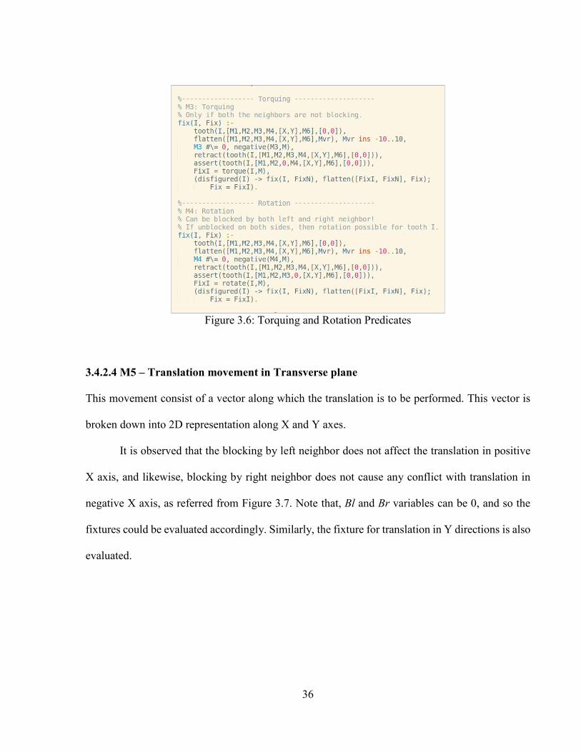
3.4.2.3 M3 – Torquing and M4 – Rotation

Torquing and Rotation for a tooth, refer Figure 3.6, it is desirable to have unblocked conditions on

either side. So, a tooth is performed with the relevant fixture out of these two only if the tooth is

unblocked. If it is even blocked by one of the adjacent tooth, the fixture is not performed. Thus,

one has to have to fix the blocking neighbor first and then try to perform these fixtures. Note that

the torquing can be performed in the both sagittal and frontal plane. Rotation is recommended only

if there is no tipping or torquing needed for a tooth. Besides, Rotation as well as Torquing does

not affect the change in the center of the tooth.

Figure 3.5: Root Tipping Predicate

36

3.4.2.4 M5 – Translation movement in Transverse plane

This movement consist of a vector along which the translation is to be performed. This vector is

broken down into 2D representation along X and Y axes.

It is observed that the blocking by left neighbor does not affect the translation in positive

X axis, and likewise, blocking by right neighbor does not cause any conflict with translation in

negative X axis, as referred from Figure 3.7. Note that, Bl and Br variables can be 0, and so the

fixtures could be evaluated accordingly. Similarly, the fixture for translation in Y directions is also

evaluated.

Figure 3.6: Torquing and Rotation Predicates

37

3.4.2.5 M6 – Intrusion/ Extrusion

The level of intrusion (pushing the tooth towards to bone) or extrusion (pulling the tooth away

from the bone) depends upon the deviation of the tooth in Z axis. Z axis is perpendicular to the

transverse plane. And the Z-deviation determines the level of intrusion/ extrusion by comparing

the model to be diagnosed with the correct model as in Figure 3.8.

Eventually all the values in the predicate are fixed to be 0, so that the model or dentition

has no irregularities left. This process continues until we find a fixture for all the deviations for

every tooth in the model.

These predicates combine to form a logic program which could serve as an input in a

predicate called state. The state is evaluated and according the sequence of fixtures is generated.

Figure 3.7: Translation in Transverse Plane Predicates

38

A state consists of assertions about initial dentition and for each tooth indexed from 0 to N-1,

where N is total number of teeth in the arch form.

The main search predicate, as in Figure 3.9, goes through all the possibilities to fix the

tooth sequentially by considering the blocking constraints. It evaluates the tooth which has no

blocking. The model needs to have at-least a single tooth that has no blocking, in our case which

is the most posterior molar (second or third molar depending upon the dentition).

Figure 3.8: Intrusion/ Extrusion Predicate

Figure 3.9: Main search Predicate

39

3.5 Test Cases and Results

• Test Case 1: As simple as no deviation at all, as shown in Figure 3.10.

• Test Case 2 and 3: Case 2 is a simple single deviation for a tooth at index 8. Case 3 is

multiple deviations for teeth with no blocking constraints, as shown in Figure 3.11.

Figure 3.10: Input and Output - Test Case 1

Figure 3.11: Input and Output - Test Case 2 and 3

40

• Test Case 4: With a simple blocking of tooth(7, _) to tooth(8, _), as shown in Figure 3.12.

• Test Case 5: Multiple blocking to a single tooth – tooth(8, _, [1,1]) as in Figure 3.13.



41

• Test Case 6: Multiple triplets of multiple blocking constraints as in Figure 3.14.

• Test Case 7: A complex dentition with multiple blocking constraints as in Figure 3.15.



42

CHAPTER 4

SEGMENTATION AND DATA GENERATION

4.1 Background

The most challenging part of this study is to go through an actual 3D model to figure out the

relevant parameters for the optimization program we saw in Chapter 3.

In order to generate the required data for each model, we need to know the orientation of

each irregular tooth with its correct orientation. The parameters indicate the deviations for each

tooth from its expected orientation.

The general 3D model looks like the Figure 4.1 and Figure 4.2.

These models are obtained by technologies which are available in the market. It uses

cephalometric tracing [9] which could generate the STL file of segmented teeth and bone structures

from a CBCT (Cone Beam Computed Tomography) file. These CBCT scans are computed using

divergent X-rays, forming a cone. The generated STL files have been used for computation of

parameters in this study.

Figure 4.1: O4R8 3D model in STL format

(Meshlab) with Gingiva

Figure 4.2: O3M6 3D model in STL format

(Meshlab) with supplemental

43

These 3D models were studied using Meshlab and Meshlab server [20] [21] to automate

the segmentation of these pre-processed file. Due to some challenges in the scripting the manual

process in Meshlab server, there is a shift in usage of Blender from Meshlab. Blender provides

more control over the processing and has been popular in professional community. Figure 4.3

shows a 3D STL model in Blender application.

Figure 4.3: A sample 3D model in Blender

44

4.2 Blender and Python (bpy)

Blender is equipped with large API (Application Programming Interface) available with many

modules with extensive documentation on its application [1]. To name a few – Math Types &

Utilities (mathutils), Blender Python (bpy), Geometry Utilities (mathutils.geometry), BMesh

Module (bmesh), OpenGL Wrapper (bgl).

The most widely used module is Blender Python (bpy). Python is an interactive, interpreted

and object-oriented programming language. It has exceptional potential with a clear syntax for

incorporating modules, exceptions, dynamic typing, classes, and so on.

To extend the Blender functionalities, Python scripts are powerful and versatile to script

repetitive tasks in the areas of animation, rendering, import/ export, object creation, modification

and data extraction. Blender Python API have been referenced for writing scripts to automate the

task in this chapter. One can create add-ons to encapsulate and distribute scripts, or even share the

scripts to be included in official Blender distribution.

The Blender Python API has components which are still in development phase, like mesh

creation and editing functions, which could be subject to change in future. Although, there are

more stable areas which are unlikely to be changed and could be used by any development research

group.

We use the Blender version 2.79b, Hash: f4dc9f9d68b, in a Linux environment with ubuntu

16.04 LTS (64-bit) operating system. It uses Intel® UHD Graphics 620 (Kabylake GT2) for

graphics and Intel® Core™ i5-8250U CPU @ 1.60GHz × 8 as it’s processor.

45

4.2.1 Python in Blender

Blender can be invoked from the terminal using its blender executable. The above screen appears

as we see the startup screen in the Blender application. Blender has an embedded Python interpreter

[2]. It is loaded as the application is running staying active until we close. This interpreter is used

to implement certain python scripts with Blender’s internal tools.

It is more like a Python environment, and one could start off with writing code from

tutorials on how to write python scripts. Blender provides bpy and mathutils to be imported in the

python scripts, which are executed with this embedded interpreter, to give access to Blender’s data,

classes, and functions.

Here is a simple example which demonstrates a translation of a vertex attached to an object

(default object) Cube.

import bpy

bpy.data.objects[“Cube”].data.vertices[0].co.x += 1

This can modify the internal data directly. This script can be saved in a file to be executed

from a Text Editor (bottom middle window in the above image), or it can be executed in the

interactive Python console (bottom left window with black background in the above image).

It is advisable to load the scripts in the Text Editor and run, but one could use any of these

3 methods to execute the scripts -

1. Load the script in the Text Editor and press Run Script.

2. Type or paste the script into the interactive Python console.

46

3. Execute a python file with Blender from the command line. For example:

$ Blender2.79b/blender --python /home/rahul/AI-Based-

Orthodontics/Samples/Q3Z7-L/BPY01.Segmentation.Script.py

4.3 Conventions about the input 3D models

• Each file represents a 3D teeth model in .STL format.

• NAMING CONVENTION of the files:

Consider the example files - O3M6.L1.013.stl, and O3M6.L1.Suppl.027.stl

◦ First four characters represent the patient number.

Here, O3M6 is patient number.

◦ Again, after the 'dot' we have first character as 'L' for lower and 'U' for upper teeth

model. This is followed by '1' (indicating crooked model) or by '2' (indicating fixed

model).

◦ After the 'dot' separator we have 'Suppl' as optional to only those files which has the

complete root model. We can also have 'Ging' as optional to those files with gingiva

(gums) present in the 3D models.

◦ After the 'dot', we have last three digits determining the number (N - 1) where N is the

total number of teeth (or the number of meshes) in the 3D model file. Here, as we’ve

N = 14 so, we add '.013' in the end for normal O3M6.L1.013.stl file.

Thus, O3M6.L1.Suppl.027.stl tells us that this is the model for the patient 'O3M6' which is

supplemental which is lower crooked model having 14 teeth with 28 different meshes.

47

Few models as an example opened as in Blender:

O3M6-L1: Figure 4.4 and Figure 4.5 shows normal and supplemental model respectively.

O4R8-L1: Figure 4.6 and Figure 4.7 shows normal and supplemental model respectively.

Figure 4.4: O3M6.L1.013.stl

Figure 4.5: O3M6.L1.Suppl.013.stl

Figure 4.6: O4R8.L1.015.stl

Figure 4.7: O4R8.L1.Ging.015.stl

48

4.4 Series of Python Scripts

There is a series of scripts, as shown in Figure 4.8, through which a 3D model is passed through

to generate the parameters we require for the optimization algorithm.

Each script file uses a set of input and produces an output. Overall, the first script uses the

plain non-segmented 3D model for a patient with irregularities and fixed versions, whereas the last

script generates the parameters required.

These scripts generate segmented files creating new directories. These scripts could be

executed from a batch file as we can run python scripts in the blender environment. The convention

for naming the input and output files is strictly followed throughout this pipeline so that the

indexing is as expected for the subsequent programs.

Scripts BPY02 and BPY03 uses two different add-ons which are available freely [23].

BPY02 uses BTrace which is pre-installed, whereas BPY03 uses Min Bounding Box [24] [25]

which is requires manual installation.

Figure 4.8: Block Diagram of Python Scripts

49

4.4.1 BPY01.Segmentation.Script.py

Given a 3D model (with no gingiva, or supplemental), this script segments the meshes from the

pre-processed STL file as shown in Figure 4.9 and Figure 4.10. These meshes were present in the

given single STL file. After execution of this script, each tooth is saved into new STL file with

mesh of its own.

Figure 4.9: I/O for BPY01

Figure 4.10: Output of BPY01 in Blender

50

4.4.2 BPY02.Spline.Generation.py

Once the 3D model is segmented, from Figure 4.11, the individual meshes are imported back to

produce the spline subsequently. Their centers are extracted so that the BTrace add-on is executed

with Objects Connect tool, connecting the centers of these meshes sequentially. Note that this

curve is then made smooth and stored in the STL file again as in Figure 4.12.


Figure 4.12: Output for BPY02

51

4.4.3 BPY03.Spline.Approximation.py

The smooth spline is again imported to compute the Minimum Bounding Box for it as shown in

Figure 4.13 and Figure 4.14. It is used to further compute the rotation parameters for the 3D model.

These rotation parameters are then applied to the original 3D model to produce the rotated version

of the model.


Figure 4.14: Output for BPY03 in Blender

52

4.4.4 BPY04.New.Segmentation.py

The rotated version of the 3D model is then segmented in the similar fashion that it was segmented

in the first script, as shown in Figure 4.15 and Figure 4.16. Here, the model file is renamed as in

the above example, from O4R8.L1.015.Rotated.stl to O4R8.L1.Rot.015.stl.


Figure 4.16: Output for BPY04 in Blender

53

4.4.5 BPY05.Apprx.Z.Translation.py

As shown in Figure 4.17, the rotated and segmented models are then applied a transformation

along Z axis. The amount of translation is calculated from average Z coordinates of the centers of

these individual meshes. All these meshes are then pushed towards Z = 0 plane by the mean Z

values to give the properly aligned model as shown in Figure 4.18.


Figure 4.18: Output of BPY05 in Blender

54

4.4.6 BPY06.Generation.M5.M6.py

The final step, as in Figure 4.19, comprises of computing the deviations in terms of translation and

rotation vectors. There is visible difference in terms of translation, as seen from Figure 4.20, but

there is no tool available to discover the deviations in terms of rotation vectors.


Figure 4.20: Start and Final (Yellow) State of 3D model

55

These deviations can be stored in the required file which then further could be read into the

optimization program as shown in Figure 4.21.

These numbers indicated in the above image, in the left-hand side of the python console

window, is the outcome of the script shown in the Text Editors on the right side. These numbers

could be fit it in the tooth predicate for each of the index. For example, for ToothIndex = i,

tooth predicate will look like -

tooth(i, [M1, M2, M3, M4, [Dx[i], Dy[i]], Dz[i]], [Bl, Br]).

Figure 4.21: Output for BPY06

56

4.5 Bounding Box and Challenges

The segmentation and parameter generation has been the most challenging part of this study. The

evaluation of other parameters in the tooth predicate requires knowledge of the deviation in

rotation vectors of the 3D model [33].

tooth(i, [M1, M2, M3, M4, [Dx[i], Dy[i]], Dz[i]], [Bl, Br]).

Parameters for Crown Tipping, Root Tipping, and Torquing requires information about the

vector passing from the center (or root) to the crown of the tooth. As we have the center, the point

on the crown is to be calculated considering different surfaces for the crowns of different tooth.

Let’s call this as normal N1. Crowns may have a single cusp or up to 4-5 cusps as in case of molars.

Thus, identifying the best suitable crown point for these surfaces would yield the parameters for

M1, M2, and M3, as these movements (or deviations) rely on vertical axis of the tooth passing

through the crown.

Besides, that M4 requires to know the direction of frontal plane for the tooth. It is the

deviation vector in terms of rotation of the tooth, where normal N1 is acting as axis of rotation,

from its fixed counterpart. Let us call this as normal N2. This normal is passing through the center

and perpendicular to the frontal plane of a tooth. As you rotate a tooth, along the axis of rotation

as N1, this normal changes its angle and thus contributes to the parameter required as M4.

The boolean values for Bl and Br can be determined using simple overlapping of two

bounding boxes. As, we have normals N1 and N2, we can form a bounding box encapsulating the

mesh of a tooth. Hence, construction of this bounding box could attribute to the blocking

constraints of neighboring teeth. For example, tooth at index 7 and index 8 has an overlap, we can

further verify that by confirming whether tooth(7, _) or tooth(8, _) has non-zero deviation in

57

general direction of its neighbor. As in this case, say tooth(8, _) had a deviation on the opposite

direction of tooth(7,_), it means tooth(8, _) needs to be moved towards tooth(7, _). And thus,

tooth(7, _) would have a blocking constraint on tooth(8, _). We can further check the same for

tooth(7, _) and its neighbors. Therefore, blocking is not a two-way constraint.

Computation of remaining parameters is tricky and could be extended as an add-on in

Blender to contribute to this problem. The problem could also be simplified by determining any

other point on the mesh, assuming that the same point is determined for all different orientations

of the same mesh. Further, joining these two segments on the same source as origin or a pivot, we

can compute the deviations in the rotation of these teeth.

Though absence of other parameters is still a goal to be achieved, evaluating the

translational parameters has more impact in determining the irregularities in malocclusions as most

of the orthodontic treatment fall under the class I malocclusion [4] [5] [6] [7]. Note that, no

prediction or estimates are made in evaluation of the parameters. Thus, these parameters can be

trusted with high confidence level capturing slightest of deviation in the dentition.

58

CHAPTER 5

APPLICATIONS

5.1 Conclusion

Existing scenarios in today’s world depict cost and time as biggest challenges in the orthodontic

treatment. It is predominantly affordable to the people with higher income. Besides, no treatment

uses machine intelligence to optimize the dental plan. Instead expertise of Orthodontists is used in

evaluation of such optimization problem in most of the treatments. Thus, existing approaches tend

to have limited capabilities as they mostly rely on direct visualization. It has been found that these

estimates generated by orthodontists on a simple model could be variable, and are unrelated to

their clinical experience. Errors in estimation of crowding often lead to incorrect treatment

approaches, adding cost to the treatment, length of the care and unwanted forced biological sequel

in the dentition taking toll on natural remodeling of bone structures, affecting the treatment

outcome adversely.

We propose an approach based on logic and reasoning to model the estimation of spatial

orientation of the dentition, and generate the best solution to solve the optimization problem

considering all reasonable constraints in to our program. We use Prolog program with CLP(FD)

which is predominantly used for solving optimization problem on the constraint systems. The

problem is formalized, asserting and retracting logical facts dynamically and a solution is

generated satisfying all the constraints from the vast search space.

59

5.2 Contributions to the Research and Future work

This study has been made with an objective to make the orthodontic care reliable, affordable, and

expedite the overall treatment. It contributes to the field of Orthodontics by applying machine

intelligence from the logic-based approaches to solve the problem of finding best sequence of

fixtures as we rely on technology over visual observations, interactions, and articulation of human

capacity. The proposed solution harnesses key insights to produce reliable outcomes by

combination of the human expertise and technological aspects of AI. It also provides use case of

logic programming to solve a real-world optimization problem. Moreover, in its first attempt of

data extraction from 3D images, this study provides foundation for producing relevant information

from a set of point cloud.

Future work could be made in deriving more and more constraints from the scanned images

using advanced tools to get every bit of knowledge about the dentition. Several scripts used in this

study are used from freely available add-ons in Blender. Their usage is limited to manual

implementation in the Blender application. One can come up with automated pipeline of these

scripts to tackle semi-automatic segmentation and data generation process. Research could also be

made in identifying relevant bounding box for each individual tooth based on its shape and type.

This may involve the use of machine learning to identify the correct bounding box given an input

3D model for a tooth. This extraction of bounding box could also be achieved using another

approach involving identification of the location of the relevant crown point. It also needs another

point to identify the normal for the frontal plane. This work would ease the entire process and

provide a sound manifestation for building more applications around teeth movement.

60

5.3 Applications

The intriguing applications of AI-driven Orthodontic treatment is in the diagnosis, treatment and

monitoring phases of the dental care [22]. Such treatment provides better diagnosis by in-depth

understanding of the 2D and 3D constraints, quicker treatment plan due to solving the optimization

problem satisfying necessary constraints, and produces reliable outcomes.

AI based Orthodontics enables clinicians to utilize their time effectively making them focus

on actual treatment and monitoring the progress. This improves the capability of doctors to

diagnose more patients in the same amount of time.

It removes the responsibility of space estimation done usually by direct visualization by

most of the orthodontists, which is considered to be the most challenging part, by providing

accurate space analysis. Thus, this approach eliminates the uncertainty from the very first step –

understanding the case, in dental care.

Further, it considers the constraints provided by scanning the 3D model and then using an

optimization algorithm, plans the shortest series of fixtures required to fix the malocclusion for the

patient’s dentition. This leads to tremendous amount of cost cutting for most of the population

with minor to moderate crowding of teeth. These fixtures decide which of the patient’s teeth and

how the patient’s teeth should be moved, with 6 movements designed around the combination of

both translation and rotation of 3D objects. It leaves the decision of actual implementation of these

movements on to the expertise of an orthodontist. Thus, AI driven Orthodontic treatment would

save huge time and cost and would give reliable outcomes providing healthy as well as aesthetic

benefits.

61

BIBLIOGRAPHY

1. The Blender 2.79 Manual by the Blender Documentation Team, CC-BY-SA v4.0, April

2019. https://docs.blender.org/manual/en/latest/advanced/scripting/introduction.html

2. Blender Documentation Contents – Blender 2.79b, API Documentation. Python API Overview, April 2019. https://docs.blender.org/api/current/info_overview.html

3. Colin Wallis, Clare McNamara, Susan J. Cunningham, Martyn Sherriff, Jonathan R. Sandy, Anthony J. Ireland, How good are we at estimating crowding and how does it affect our treatment decisions?, European Journal of Orthodontics, Volume 36, Issue 4, August 2014, Pages 465–470, https://doi.org/10.1093/ejo/cjt080

4. Birgit Thilander, Lucia Pena, Clementina Infante, Sara Stella Parada, Clara de Mayorga, Prevalence of malocclusion and orthodontic treatment need in children and adolescents in Bogota, Colombia. An epidemiological study related to different stages of dental development, European Journal of Orthodontics, Volume 23, Issue 2, 1 April 2001, Pages 153–168, https://doi.org/10.1093/ejo/23.2.153

5. W. R. Proffit, H.W. Jr. Fields, L.J. Moray (1998), Prevalence of malocclusion and orthodontic treatment need in the United States: Estimates from the NHANES III survey. The International journal of adult orthodontics and orthognathic surgery. 13. 97-106.

6. Ali Borzabadi-Farahani, Anahid Borzabadi-Farahani, Faezeh Eslamipour, Malocclusion and occlusal traits in an urban Iranian population. An epidemiological study of 11- to 14-year-old children, European Journal of Orthodontics, Volume 31, Issue 5, October 2009, Pages 477–484, https://doi.org/10.1093/ejo/cjp031

7. J. A. Brunelle, M. Bhat, & J. A. Lipton (1996). Prevalence and Distribution of Selected Occlusal Characteristics in the US Population, 1988–1991. Journal of Dental Research, 75(2_suppl), 706–713. https://doi.org/10.1177/002203459607502S10

8. American Association of Orthodontists, April 2019. https://www.aaoinfo.org/

9. Orca Dental AI, Orthodontics: Cephalometric Analysis and Teeth Segmentation, April 2019. https://orca-ai.com/solutions/orthodontics/

10. Market research by IBISWorld, April 2019. https://www.ibisworld.com/industry-trends/specialized-market-research-reports/life-sciences/health-practitioners/orthodontists.html

https://docs.blender.org/manual/en/latest/advanced/scripting/introduction.html

https://docs.blender.org/api/current/info_overview.html

https://doi.org/10.1093/ejo/cjt080

https://doi.org/10.1093/ejo/23.2.153

https://doi.org/10.1093/ejo/cjp031

https://doi.org/10.1177/002203459607502S10

https://www.aaoinfo.org/

https://orca-ai.com/solutions/orthodontics/

https://www.ibisworld.com/industry-trends/specialized-market-research-reports/life-sciences/health-practitioners/orthodontists.html



62

11. Uniform Teeth, How it Works, Teeth Straightening, April 2019. https://www.uniformteeth.com/how-it-works/

12. Candid, How Candid Works, Teeth Straightening and Whitening, April 2019. https://www.candidco.com/how-it-works/

13. Smile Direct Club, How We Straighten Your Teeth At Home, April 2019. https://smiledirectclub.com/how_it_works/

14. Orthly, Invisible Aligners, April 2019. https://www.orthly.com/#how-it-works

15. Different types of malocclusions, by Total Orthodontics Ltd https://www.totalorthodontics.co.uk/different-types-of-malocclusions/

16. Different types of malocclusions, by Shaw Orthodontics, July 2018 https://shawsmiles.com/different-types-of-malocclusions/

17. Orthodontics: https://en.wikipedia.org/wiki/Orthodontics

18. Vickie Parrish Foster, “An Overview of Dental Anatomy,” April 2019. https://www.dentalcare.com/en-us/professional-education/ce-courses/ce500/toc

19. Maged Sultan Alhammadi, Esam Halboub, Mona Salah Fayed, Amr Labib, Chrestina El-Saaidi, Global distribution of malocclusion traits: A systematic review, 2018 Nov-Dec; 23(6): 40.e1–40.e10., Dental Press Journal of Orthodontics, PMCID: PMC6340198 PMID: 30672991 doi: 10.1590/2177-6709.23.6.40.e1-10.onl https://www.ncbi.nlm.nih.gov/pubmed/30672991

20. Meshlab Server Command Man Page https://www.mankier.com/1/meshlabserver

21. Visual Computing, MeshLab, 2012. https://sourceforge.net/p/meshlab/discussion/499533/thread/63bd8f30/

22. Dr. C. William Dabney, “Artificial Intelligence (AI) and Orthodontics – can you imagine where we will be in the very near future?” Rocky Mountain Orthodontics, Nov 2017. https://www.orthopracticeus.com/technology/artificial-intelligence-ai-orthodontics-can-imagine-will-near-future

23. Stack Exchange Inc., Blender Stack Exchange, April 2019. https://blender.stackexchange.com/questions/

24. Patrick Moore, Object Bounding Box, blenderartists.org, Mar 2015. https://blenderartists.org/t/addon-minimum-bounding-volume/635618

https://www.uniformteeth.com/how-it-works/

https://www.candidco.com/how-it-works/

https://smiledirectclub.com/how_it_works/

https://www.orthly.com/#how-it-works

https://www.totalorthodontics.co.uk/different-types-of-malocclusions/

https://shawsmiles.com/different-types-of-malocclusions/

https://en.wikipedia.org/wiki/Orthodontics

https://www.dentalcare.com/en-us/professional-education/ce-courses/ce500/toc

https://dx.doi.org/10.1590%2F2177-6709.23.6.40.e1-10.onl

https://www.ncbi.nlm.nih.gov/pubmed/30672991

https://www.mankier.com/1/meshlabserver

https://sourceforge.net/p/meshlab/discussion/499533/thread/63bd8f30/

https://www.orthopracticeus.com/technology/artificial-intelligence-ai-orthodontics-can-imagine-will-near-future

https://www.orthopracticeus.com/technology/artificial-intelligence-ai-orthodontics-can-imagine-will-near-future

https://blender.stackexchange.com/questions/

https://blenderartists.org/t/addon-minimum-bounding-volume/635618

63

25. Godfried T. Toussaint, “Solving geometric problems with rotating calipers,” Proceedings of IEEE MELECON’83, Athens, Greece, May 1983. http://www-cgrl.cs.mcgill.ca/~godfried/research/calipers.html

26. Marcus Triska, “The Power of Prolog,” April 2019. https://www.metalevel.at/prolog

27. SWI-Prolog.org, SWI-Prolog library(CLPFD), April 2019. http://www.swi-prolog.org/pldoc/man?section=summary-lib-clpfd

28. Anne Ogborn, “CLP(FD) Constraint Logic Programming over Finite Domains” Tutorial, Dec 2017. http://www.pathwayslms.com/swipltuts/clpfd/clpfd.html

29. Helmut Simonis, “Constraint Logic Programming”, COSYTEC SA, Feb 2008. http://www.utdallas.edu/~gupta/courses/lp/clp-tutorial.pdf

30. L. Sterling and E. Shapiro, “The Art of Prolog Advanced Programming Techniques”, 2nd Edition, The MIT Press Cambridge, 1999.

31. Ulf Nilsson and Jan Maluszyński, “Logic, Programming and Prolog,” 2nd Edition, 2000. http://www.ida.liu.se/~ulfni/lpp

32. John McCarthy, “What is Artificial Intelligence?” Nov 2007. http://jmc.stanford.edu/articles/whatisai/whatisai.pdf

33. G. Scott Owen, “Modeling in Computer Graphics,” July 1999. https://www.siggraph.org/education/materials/HyperGraph/modeling/cgmodel.htm

34. Zach, Richard, "Hilbert's Program", The Stanford Encyclopedia of Philosophy (Spring 2016 Edition), Edward N. Zalta (ed.). https://plato.stanford.edu/archives/spr2016/entries/hilbert-program/

35. Raatikainen, Panu, "Gödel's Incompleteness Theorems", The Stanford Encyclopedia of Philosophy (Fall 2018 Edition), Edward N. Zalta (ed.). https://plato.stanford.edu/archives/fall2018/entries/goedel-incompleteness/

36. J. A. Robinson, “A Machine-Oriented Logic based on the Resolution Principle”, Jan 1965, Journal of the ACM. 12(1): 23-41 DOI: 10.1145/321250.321253

37. Herbrand, Jaques, Recherches sur la théorie de la démonstration, 1930.

http://www-cgrl.cs.mcgill.ca/%7Egodfried/research/calipers.html

http://www-cgrl.cs.mcgill.ca/%7Egodfried/research/calipers.html

https://www.metalevel.at/prolog

http://www.swi-prolog.org/pldoc/man?section=summary-lib-clpfd

http://www.swi-prolog.org/pldoc/man?section=summary-lib-clpfd

http://www.pathwayslms.com/swipltuts/clpfd/clpfd.html

http://www.utdallas.edu/%7Egupta/courses/lp/clp-tutorial.pdf

http://www.ida.liu.se/%7Eulfni/lpp

http://jmc.stanford.edu/articles/whatisai/whatisai.pdf

https://www.siggraph.org/education/materials/HyperGraph/modeling/cgmodel.htm

https://plato.stanford.edu/archives/spr2016/entries/hilbert-program/

https://plato.stanford.edu/archives/fall2018/entries/goedel-incompleteness/

https://doi.org/10.1145%2F321250.321253

64

38. R. Kowalski, "Predicate Logic as Programming Language", in Proceedings IFIP Congress, Stockholm, North Holland Publishing Co., 1974, pp. 569–574. Reprinted in Computers for Artificial Intelligence Applications, (eds. B. Wah and G. J. Li), IEEE Computer Society Press, Los Angeles, 1986, pp. 68–73.

39. M. Van Emden and R. Kowalski, "The Semantics of Predicate Logic as a Programming Language", in Journal of the ACM, Vol. 23, No. 4, 1976, pp. 733–742.

65

BIOGRAPHICAL SKETCH

Rahul Nalawade was born in Paithan, Maharashtra, India. After completing his school education,

he joined Indian Institute of Information Technology, Vadodara. During his bachelor’s degree,

Rahul was employed by Tata Consultancy Services as a Summer SDE Intern in 2016. He

completed his bachelor’s, as a part of the pioneering batch of the Institute in 2017. He then decided

to pursue a master’s degree to enrich his knowledge about Artificial Intelligence, Machine

Learning and Natural Language Processing. He enrolled in the Master of Science in Computer

Science program at The University of Texas at Dallas in Fall of 2017.

CURRICULUM VITAE


EDUCATION

Master of Science in Computer Science (GPA 3.58/4) Expected May 2019

Thesis: AI Based Orthodontics

The University of Texas at Dallas, Texas, USA

Bachelor of Technology in Computer Science May 2017

Indian Institute of Information Technology Vadodara, Gujarat, India

SKILLS

Programming Languages: Java, Python, Shell Scripting, C++, C, Prolog, LISP

Web Technologies: HTML5, CSS3, JavaScript, PHP, JSON, JSP, JQuery, RESTful, SOAP

Database: SQL, PostgreSQL, MySQL, PL/SQL, RDBMS, Oracle SQL Developer

Software Tools: Terminal, Matlab, GitHub, MeshLab, Blender (bpy), PyOpenGL,

PhpMyAdmin, NLTK, Spacy

Others: Unix/ Linux, Agile, Object Oriented Programming and Design, Multi-threading, SDLC,

Technical Writing, Socket Programming, Answer Set Programming

WORK EXPERIENCE

SDE Intern Tata Consultancy Services, Gandhinagar, India May 2016 – July 2016

Team and Product: SAP ICC - Centralized Dashboard

RESEARCH INTERESTS

My research interests mainly include Artificial Intelligence, Machine Learning, Algorithm

Design, Natural Language Processing, and Logic Programming.

LANGUAGES

My mother tongue is Marathi. I’m also fluent in Hindi and English. I can understand Spanish and

can have conversational mostly revolving around soccer.

ai based orthodontics by rahul shankarrao nalawade

Documents