additive coefficient modeling via polynomial spline
TRANSCRIPT
ADDITIVE COEFFICIENT MODELING VIA
POLYNOMIAL SPLINE
Lan Xue and Lijian Yang
Michigan State University
Abstract : A flexible nonparametric regression model is considered in which the response de-pends linearly on some covariates, with regression coefficients as additive functions of other co-variates. Polynomial spline estimators are proposed for the unknown coefficient functions, withoptimal univariate mean square convergence rate under geometric mixing condition. Consistentmodel selection method is also proposed based on a nonparametric Bayes Information Criterion(BIC). Simulated and real data examples demonstrate that the polynomial spline estimators arecomputationally efficient and also as accurate as the existing local polynomial estimators.
Short Running Title. Additive Coefficient Model
Key words and phrases: AIC, Approximation space, BIC, German real GNP, knot, meansquare convergence, spline approximation
1. Introduction
Parametric regression models are based on the assumption that their regression functions follow apre-determined parametric form with finitely many unknown parameters. A wrong model can leadto excessive estimation biases and erroneous inferences. In contrast, nonparametric models imposeless stringent assumptions on the regression functions. General nonparametric models, however,need large sample sizes to obtain reasonable estimators when the predictors are high dimensional.Much effort has been made to alleviate the “curse of dimensionality” by imposing appropriatestructures on the regression function.
Of special importance is the varying coefficient model (Hastie & Tibshirani 1993), whoseregression function depends linearly on some regressors, with coefficients as smooth functions ofother predictor variables, called tuning variables. A special type of varying coefficient model iscalled functional coefficient model by Chen & Tsay (1993b), in which all tuning variables are thesame and univariate. It was studied in the time series context by Cai, Fan & Yao (2000) and Huang& Shen (2004). Xue & Yang (2005a) extended the functional coefficient model to the case whenthe tuning variable is multivariate, with additive structure on regression coefficients to avoid the
“curse of dimensionality”. The regression function of the new additive coefficient model is
m (X,T) =d1∑
l=1
αl (X) Tl, αl (X) = αl0 +d2∑
s=1
αls (Xs) , (1.1)
in which the predictor vector (X,T) ∈ Rd2 × Rd1 , with X = (X1, ..., Xd2)T ,T =(T1, . . . , Td1)
T .This additive coefficient model includes as special cases the varying/functional coefficient models,as well as additive model (Chen & Tsay 1993a, Hastie & Tibshirani 1990) and linear regressionmodel, see Xue & Yang (2005a), which has obtained asymptotic distributions of local polynomialmarginal integration estimators of the unknown coefficients. The parameters {αl0}d1
l=1 are estimatedat the parametric rate 1/
√n, and the nonparametric functions {αls (xs)}d1,d2
l=1,s=1 are estimated atthe univariate smoothing rate. Due to integration step and its ‘local’ nature, the kernel methodin Xue & Yang (2005a) is computationally expensive. Based on a sample of size n, to estimatethe coefficient functions {αl (x)}d1
l=1 in (1.1) at any fixed point x, a total of (d2 + 1) n least squaresestimations have to be done. So the computational burden increases dramatically as the samplesize n and the dimension of the tuning variables d2 increase.
In this paper, we propose a faster polynomial spline estimator for model (1.1). In contrast tothe local polynomial, polynomial spline is a global smoothing method. One solves only one leastsquares estimation to estimate all the components in the coefficient functions, regardless of thesample size n and the dimension of the tuning variable d2. So the computation is substantiallyreduced. As an attractive alternative to the local polynomial, polynomial spline has been used toestimate various models, for example, additive model (Stone 1985), the functional ANOVA model(Huang 1998a, b), the varying coefficient model (Huang, Wu & Zhou 2002), and additive model forweakly dependent data (Huang & Yang 2004), with asymptotic results. We have given completeproof of the polynomial spline estimators’ rate of convergence under geometric mixing condition.A major innovation is the use of approximation space with possibly unbounded basis. Huang,Wu & Zhou (2002), for instance, has imposed the assumption that T =(T1, . . . , Td1)
T in (1.1) hascompactly supported distribution to make their basis bounded. Our method, in contrast, onlyimposes mild moment conditions on T.
The paper is organized as follows. Section 2 discusses the identification issue for model (1.1).Section 3 presents the polynomial spline estimators, their L2 consistency and a model selectionprocedure based on Bayes Information Criterion (BIC). These estimation and model selectionprocedures adapt automatically to varying coefficient model (Hastie & Tibshirani 1993), functionalcoefficient model (Chen & Tsay 1993b), additive model (Hastie & Tibshirani 1990, Chen & Tsay1993a), and linear regression model, a feature not shared by any kernel type estimators. Section 4applies the methods to the simulated and empirical examples. Technical assumptions and proofsare given in the Appendix.
2. The Model
Let {(Yi,Xi,Ti)}ni=1 be a sequence of strictly stationary observations, with univariate response Yi,
d2 and d1 variate predictors Xi and Ti. With unknown conditional mean and variance functions
2
m (Xi,Ti) = E (Yi|Xi,Ti) , σ2 (Xi,Ti) = var (Yi|Xi,Ti), the observations satisfy
Yi = m (Xi,Ti) + σ (Xi,Ti) εi. (2.1)
The errors {εi}ni=1 are i.i.d with E (εi|Xi,Ti) = 0, E
(ε2i |Xi,Ti
)= 1, and εi independent of
the σ-field Fi = σ {(Xj ,Tj) , j ≤ i} for i = 1, . . . , n. So the variables (Xi,Ti) can consist of eitherexogenous variables or lagged values of Yi. For the additive coefficient model, the regression functionm takes the form in (1.1), and satisfies the identification conditions that
E {αls (Xis)} = 0, 1 ≤ l ≤ d1, 1 ≤ s ≤ d2. (2.2)
The conditional variance function σ2 (x, t) is assumed to be continuous and bounded. As in mostworks on nonparametric smoothing, estimation of the functions {αls (xs)}d1,d2
l=1,s=1 is conducted oncompact sets. Without lose of generality, let the compact set be χ = [0, 1]d2 .
Following Stone (1985), p.693, the space of s-centered square integrable functions on [0, 1] is
H0s =
{α : E {α (Xs)} = 0, E
{α2 (Xs)
}< +∞}
, 1 ≤ s ≤ d2.
Next define the model space M, a collection of functions on χ×Rd1 as
M =
{m (x, t) =
d1∑
l=1
αl (x) tl; αl (x) = αl0 +d2∑
s=1
αls(xs);αls ∈ H0s
},
in which {αl0}d1l=1 are finite constants. The constraints that E {αls (Xs)} = 0, 1 ≤ s ≤ d2 ensure
unique additive representation of αl, but are not necessary for the definition of space M.In what follows, denote by En the empirical expectation, Enϕ =
∑ni=1 ϕ (Xi,Ti) /n. We
introduce two inner products on M. For functions m1,m2 ∈ M, the theoretical and empiri-cal inner products are defined respectively as 〈m1,m2〉 = E {m1 (X,T) m2 (X,T)} , 〈m1,m2〉n =En {m1 (X,T) m2 (X,T)}. The corresponding induced norms are ‖m1‖2
2 = Em21 (X,T), ‖m1‖2
2,n =Enm2
1 (X,T). The model spaceM is called theoretically (empirically) identifiable, if for any m ∈M,‖m‖2 = 0 (‖m‖2,n = 0) implies that m = 0 a.s.
Lemma 1 Under assumptions (C1) and (C2) in the Appendix, there exists a constant C > 0 suchthat
‖m‖22 ≥ C
{d1∑
l=1
(α2
l0 +d2∑
s=1
‖αls‖22
)}, ∀ m =
d1∑
l=1
(αl0 +
d2∑
s=1
αls
)tl ∈M.
Hence for any m ∈ M, ‖m‖2 = 0 implies αl0 = 0, αls = 0 a.s., for all 1 ≤ l ≤ d1, 1 ≤ s ≤ d2.Consequently the model space M is theoretically identifiable.
Proof. Let Al(X) = αl0 +d2∑
s=1αls(Xs),A(X) = (A1(X), . . . , Ad1(X))T . Under assumption (C2)
‖m‖22 = E
[d1∑
l=1
{αl0 +
d2∑
s=1
αls(Xs)
}Tl
]2
= E[A(X)TTTTA(X)
]
≥ c3E[A(X)TA(X)
]= c3E
d1∑
l=1
{αl0 +
d2∑
s=1
αls(Xs)
}2
3
which, by (2.2), is c3
[∑d1l=1 α2
l0 +∑d1
l=1 E{∑d2
s=1 αls(Xs)}2
]. Applying Lemma 1 of Stone (1985)
‖m‖22 ≥ c3
[d1∑
l=1
α2l0 + {(1− δ)/2}d2−1
d1∑
l=1
d2∑
s=1
Eα2ls(Xs)
],
where δ = (1− c1/c2)1/2 with 0 < c1 ≤ c2 as specified in assumption (C1). By takingC = c3 {(1− δ)/2}d2−1, the first part is proved. To show identifiability, notice that for anym =
∑d1l=1
(αl0 +
∑d2s=1 αls
)tl ∈ M, with ‖m‖2 = 0, we have
0 = E
[d1∑
l=1
{αl0 +
d2∑
s=1
αls(Xs)
}Tl
]2
≥ C
[d1∑
l=1
α2l0 +
d1∑
l=1
d2∑
s=1
E{α2
ls(Xs)}]
,
which entails that al0 = 0 and αls(Xs) = 0 a.s. for all 1 ≤ l ≤ d1, 1 ≤ s ≤ d2, or m = 0 a.s. ¥
3. Polynomial Spline Estimation
3.1 The estimators
In this paper, denote by Cp ([0, 1]) the space of p-times continuously differentiable functions. Foreach of the tuning variable direction, i.e. s = 1, . . . , d2, a knot sequence ks,n with Nn interior knotsis introduced
ks,n = {0 = xs,0 < xs,1 < · · · < xs,Nn < xs,Nn+1 = 1} .
For an integer p ≥ 1, define ϕs = ϕp([0, 1] , ks,n), a subspace of Cp−1 ([0, 1]) consisting of func-tions that are polynomial of degree p (or less) on intervals [xs,i, xs,i+1), i = 0, . . . , Nn − 1, and[xs,Nn , xs,Nn+1]. Functions in ϕs are called polynomial splines, which are piecewise polynomialsconnected smoothly on the interior knots. So a polynomial spline with degree p = 1 is a continuouspiecewise linear function, etc. The space ϕs is determined by the polynomial degree p and theknot sequence ks,n. Let hs = hs,n = maxi=0,...,Nn |xs,i+1 − xs,i|, called mesh size of ks,n, and defineh = maxs=0,...,d2 hs, the overall smoothness measure.
Lemma 2 For 1 ≤ s ≤ d2, define ϕ0s = {gs : gs ∈ ϕs, Egs (Xs) = 0}, the space of centered polyno-
mial splines. There exists a constant c > 0, so that for any αs ∈ H0s ∩ Cp+1 ([0, 1]), there exists a
gs ∈ ϕ0s, such that ‖αs − gs‖∞ ≤ c
∥∥∥α(p+1)s
∥∥∥∞
hp+1s .
Proof. According to de Boor (2001), p.149, there exists a constant c > 0 and spline functiong∗s ∈ ϕs, such that ‖αs − g∗s‖∞ ≤ c
∥∥∥α(p+1)s
∥∥∥∞
hp+1s . Note next that |Eg∗s | ≤ |E (g∗s − αs)|+ |Eαs| ≤
‖g∗s − αs‖∞. Thus for gs = g∗s − Eg∗s ∈ ϕ0s, one has
‖αs − gs‖∞ ≤ ‖αs − g∗s‖∞ + Eg∗s ≤ 2c∥∥∥α(p+1)
s
∥∥∥∞
hp+1s . ¥
Lemma 2 entails that if the functions {αls (xs)}d1,d2
l=1,s=1 in (1.1) are smooth, they are approx-
imated well by centered splines{gls (xs) ∈ ϕ0
s
}d1,d2
l=1,s=1. As the definition of ϕ0
s depends on the
4
unknown distribution of Xs, the empirically defined space ϕ0,ns = {gs : gs ∈ ϕs, En(gls) = 0} is
used. Intuitively, function m ∈M is approximated by some function from the approximate space
Mn =
{mn (x, t) =
d1∑
l=1
gl (x) tl; gl (x) = αl0 +d2∑
s=1
gls(xs); gls ∈ ϕ0,ns
}.
Given observations {(Yi,Xi,Ti)}ni=1 from model (2.1) , the estimator of the unknown regression
function m is defined as its ‘best’ approximation from Mn,
m = argminmn∈Mn
n∑
i=1
{Yi −mn (Xi,Ti)}2 . (3.1)
To be precise, write Jn = Nn + p, and let {ws,0, ws,1, . . . , ws,Jn} be a basis of the spline spaceϕs, for 1 ≤ s ≤ d2. For example, the truncated power basis is used in the implementation
{1, xs, . . . , x
ps, (xs − xs,1)
p+ , . . . , (xs − xs,Nn)p
+
},
in which (x)p+ = (x+)p. Let w = {1, w1,1, . . . , w1,Jn , . . . , wd2,1, . . . , wd2,Jn}, then {wt1, . . . ,wtd1} is
a Rn = d1 {d2Jn + 1} dimensional basis of Mn, and (3.1) amounts to
m (x, t) =d1∑
l=1
cl0 +
d2∑
s=1
Jn∑
j=1
cls,jws,j (xs)
tl, (3.2)
in which the coefficients {cl0, cls,j , 1 ≤ l ≤ d1, 1 ≤ s ≤ d2, 1 ≤ j ≤ Jn} minimize the sum of squares
n∑
i=1
Yi −
d1∑
l=1
cl0 +
d2∑
s=1
Jn∑
j=1
cls,jws,j (Xis)
Til
2
(3.3)
with respect to {cl0, cls,j , 1 ≤ l ≤ d1, 1 ≤ s ≤ d2, 1 ≤ j ≤ Jn}. Note that Lemma A.5 entails that,with probability approaching one, the sum of squares in (3.3) has a unique minimizer. For 1 ≤l ≤ d1, 1 ≤ s ≤ d2, denote α∗ls(xs) =
∑Jnj=1 cls,jws,j(xs). Then the estimators of {αl0}d1
l=1 and{αls (xs)}d1,d2
l=1,s=1 in (1.1) are given as
αl0 = cl0 +d2∑
s=1
Enα∗ls, 1 ≤ l ≤ d1;
αls(xs) = α∗ls(xs)− Enα∗ls 1 ≤ l ≤ d1, 1 ≤ s ≤ d2, (3.4)
where {αls(xs)}d1,d2
l=1,s=1 are empirically centered to consistently estimate the theoretically centeredfunction components in (1.1). These estimators are determined by the knot sequences {ks,n}d2
s=1
and the polynomial degree p, which relates to the smoothness of the regression function. We willrefer to an estimator by its degree p. For example, a linear spline fit corresponds to p = 1.
Theorem 1 Under assumptions (C1)-(C5) in the Appendix, if αls ∈ Cp+1 ([0, 1]) , for 1 ≤ l ≤d1, 1 ≤ s ≤ d2, one has
‖m−m‖2 = Op
(hp+1 +
√1/nh
),
max1≤l≤d1
|αl0 − αl0|+ max1≤l≤d1,1≤s≤d2
‖αls − αls‖2 = Op
(hp+1 +
√1/nh
).
5
Theorem 1 entails that the optimal order of h is n−1/(2p+3), in which case ‖αls − αls‖2 =Op
(n−1/(2p+3)
), which is the same rate of the mean square errors as the marginal integration
estimators in Xue & Yang (2005a).
3.2 Knot number selection
An appropriate selection of the knot sequence is important to efficiently implement the proposedpolynomial spline estimation method. Stone (1986) found that the number of knots is more crucialthan its location. Thus we discuss an approach to select the number of interior knots Nn using theAIC criteria. For knots location, we use either equally spaced knots (the same distance betweenany adjacent knots), or quantile knots (sample quantiles with the same number of observationsbetween any two adjacent knots).
According to Theorem 1, the optimal order of Nn is n1/(2p+3). Thus we propose to select the‘optimal’ Nn denoted as Nopt
n from the set of integers in [0.5Nr,min (5Nr, T b)] with Nr = n1/(2p+3)
and Tb = {n/ (4d1)− 1} /d2 which ensures the total number of parameters in the least squareestimation is less than n/4.
To be specific, we denote the estimator for the i-th response Yi by Yi (Nn) = m (Xi,Ti), fori = 1, · · · , n. Here m depends on the knot sequence as given in (3.2). Let qn = (1 + d2Nn) d1 bethe total number of parameters in the least square problem (3.3). Then Nopt
n is the one minimizingthe AIC value
Noptn = argmin
Nn∈[0.5Nr,min(5Nr,T b)]AIC (Nn) , (3.5)
where AIC (Nn) = log (MSE) + 2qn/n with MSE =∑n
i=1
{Yi − Yi (Nn)
}2/n.
3.3 Model selection
For the full model (1.1), a natural question to ask is whether the functions {αls (xs)}d1,d2
l=1,s=1 are allsignificant. A simpler model by setting some of {αls (xs)}d1,d2
l=1,s=1 zero may perform as well as the fullmodel. For 1 ≤ l ≤ d1, let Sl denote the set of indices of the tuning variables which are significantin the coefficient function of Tl, and S the collection of indices from all the sets Sl. The set S iscalled the model indices. In particular, the model indices of the full model is Sf = {Sf1, . . . , Sfd1},where Sfl ≡ {1, . . . , d2} , 1 ≤ l ≤ d1. For two indices S = {S1, . . . , Sd1} , S′ =
{S′1, . . . , S
′d1
}, we say
that S ⊂ S′ if and only if Sl ⊂ S′l, for all 1 ≤ l ≤ d1 and Sl 6= S′l, for some l. The goal is to selectthe smallest sub-model with indices S ⊂ Sf , which gives the same information as the full additivecoefficient model. Following Huang & Yang (2004), Akaike Information Criterion (AIC) and BayesInformation Criterion (BIC) are considered.
For a submodel mS with indices S = {S1, . . . , Sd1}, let Nn,S be the number of interiorknots used to estimate the model mS and Jn,S = Nn,S + p. As in the full model estimation,let {cl0, cls,j , 1 ≤ l ≤ d1, s ∈ Sl, 1 ≤ j ≤ Jn,S} be the minimizer of the sum of squares
n∑
i=1
Yi −
d1∑
l=1
cl0 +
∑
s∈Sl
Jn,S∑
j=1
cls,jws,j (Xis)
Til
2
. (3.6)
6
Define
mS (x, t) =d1∑
l=1
cl0 +
∑
s∈Sl
Jn,S∑
j=1
cls,jws,j (xs)
tl. (3.7)
Denote Yi,s = mS (Xi,Ti),i = 1, · · · , n, MSES =∑n
i=1
(Yi − Yi,s
)2/n, qS =
∑d1l=1 {1 + # (Sl) Jn,s},
the total number of parameters in (3.6). Then the submodel is selected with the smallest AIC (orBIC) values, defined as AICS = log (MSES) + 2qS/n, BICS = log (MSES) + log (n) qS/n.
Let S0 and S be the index set of the true model and the selected model respectively. Theoutcome is defined as correct fitting, if S = S0; overfitting, if S0 ⊂ S; and underfitting, if S0 6 ⊂S,that is, S0l 6 ⊂Sl, for some l. For either overfitting or underfitting, we denote S 6= S0.
Theorem 2 Under the same conditions as in Theorem 1, and Nn,S ³ Nn,S0 ³ n1/(2p+3), the BICis consistent: for any S 6= S0, limn→∞ P (BICS > BICS0) = 1, hence limn→∞ P
(S = S0
)= 1.
The condition that Nn,S ³ Nn,S0 is essential for the BIC to be consistent. As a referee pointedout, the number of parameters qS depends on the number of knots and the number of additiveterms used in the model function. To ensure BIC consistency, roughly the same sufficient numberof knots should be used to estimate the various models so that qS depends only on the number offunctions terms. In the implementation, we have used the same number of interior knots Nopt
n (see(3.5), the optimal knot number for the full additive coefficient model) in the estimation of all thesubmodels.
4. Examples
In this section, we first analyze two simulated data sets with an i.i.d. and time series set-uprespectively. Both data sets have sample sizes n = 100, 250 and 500, and 100 replications. Laterthe proposed methods are successfully applied to an empirical example: West German real GNP.
The performance of the function estimators is assessed by the averaged integrated squarederror (AISE). Denoting the estimator of αls in the i-th replication as αi,ls, and {xm}ngrid
m=1 the gridpoints where the functions are evaluated, we define
ISE(αi,ls) =1
ngrid
ngrid∑
m=1
{αi,ls(xm)− αls(xm)}2 and AISE(αls) =1
100
100∑
i=1
ISE(αi,ls).
4.1 Simulated example 1
The data are generated from the model
Y = {c1 + α11 (X1) + α12 (X2)}T1 + {c2 + α21 (X1) + α22 (X2)}T2 + ε,
with c1 = 2, c2 = 1 and α11 (x) = sin {2(4x− 2)} + 2 exp{−2(x− 0.5)2
}, α12 (x) = x, α21 (x) =
sin (x), α22 (x) = 0. The vector X = (X1, X2)T is uniformly distributed on [−π, π]2 independent of
the standard bivariate normal T = (T1, T2)T . The error ε is a standard normal variable independent
of (X,T).
7
The functions are estimated by linear spline (p = 1), cubic spline (p = 3) and the marginalintegration method of Xue & Yang (2005a). For s = 1, 2, let xi
s,min, xis,max denote the smallest
and largest observation of the variable xs in the i-th replication. Knots are placed evenly on theintervals
[xi
s,min, xis,max
], with the number of interior knots Nn selected by AIC as in subsection
3.2. The functions {αls}2,2l=1,s=1 are estimated on a grid of equally-spaced points xm,m = 1, ..., ngrid
with x1 = −0.975π, xngrid= 0.975π, ngrid = 62.
Table 1 reports the means and standard errors (in the parentheses) of {cl}l=1,2 and the AISEsof {αls}s=1,2
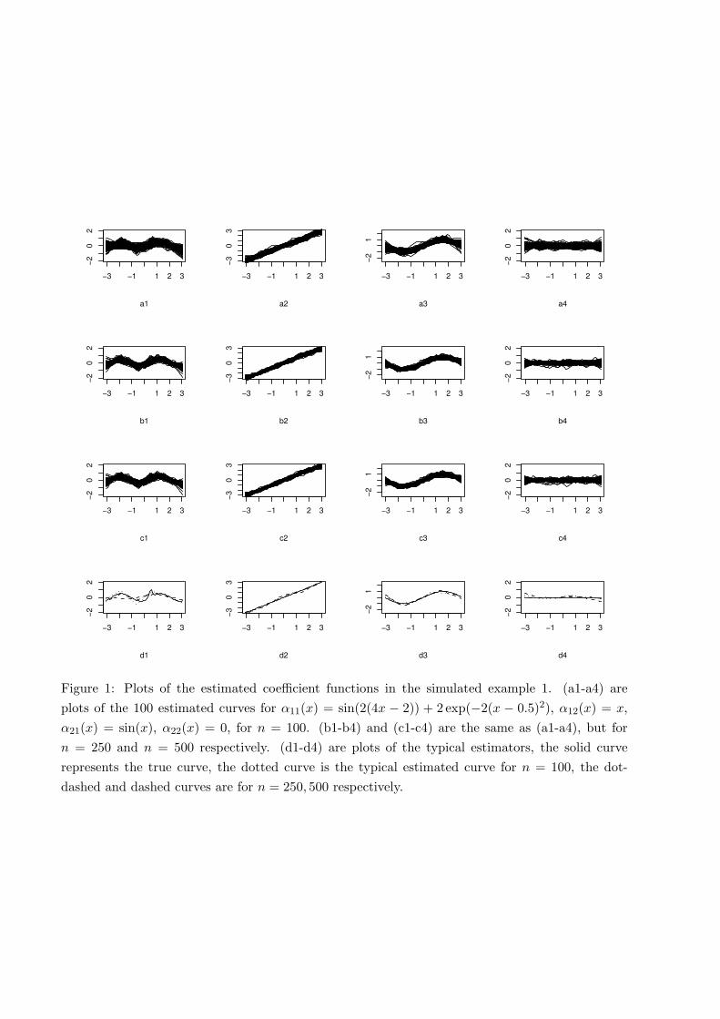
l=1,2 for all the three fits. Both spline fits (p = 1, 3) are generally comparable, with thecubic fit (p = 3) better than the linear fit (p = 1) for larger sample sizes (n = 250, 500), thestandard errors of the constant estimators and the AISEs of the function estimators decrease assamples size increases, confirming Theorem 1. The polynomial spline methods also perform betterthan the marginal integration method. Figure 1 gives the plots of the 100 cubic spline fits for allsample sizes, clearly illustrating the estimation improvements as sample size increases. Plots d1-d4of the typical estimated curves (whose ISE is the median of the 100 ISEs from the replications)seem satisfactory for sample size as small as 100.
As mentioned earlier, the polynomial spline method enjoys great computational efficiency. Ittakes polynomial spline less than 20 seconds to run 100 simulations on a Pentium 4 PC, regardlessof sample sizes. In contrast, it takes marginal integration about 2 hours to run 100 simulationswith n = 100; and about 20 hours with n = 500.
For each replication, model selection is also conducted according to the criteria proposed insubsection 3.3, for polynomial splines with p = 1, 2, 3. The model selection results are presentedin Table 2, indexed as ‘Example 1’. The BIC is rather accurate: more than 86% correct selectionwhen the sample size is as small as 100, and absolute correct selection when sample size increasesto 250 and 500, corroborating with Theorem 2 that BIC is consistent. AIC clearly tends to over-fitand never under-fits.
(Insert Table 1 about here)
(Insert Table 2 about here)
(Insert Figure 1 about here)
4.2 Simulated example 2
The data is generated from a nonlinear AR model
Yt = {c1 + α11 (Yt−1) + α12 (Yt−2)}Yt−3 + {c2 + α21 (Yt−1) + α22 (Yt−2)}Yt−4 + 0.1εt,
with i.i.d. standard normal noise εt, c1 = 0.2, c2 = −0.3 and
α11 (u) = (0.3 + u) exp(−4u2), α12 (u) = 0.3/{1 + (u− 1)4
},
a21 (u) = 0, α22 (u) = −(0.6 + 1.2u) exp(−4u2).
In each replication, a total of 1000 + n observations are generated and only the last n obser-vations are used to ensure approximate stationarity. In this example, we have used linear spline(p = 1) on the quantile knot sequences. The coefficient functions {αls}2,2
l=1,s=1 are estimated on a
8
grid of equally-spaced points on the interval [−1, 1], with the number of grid points ngrid = 41.Table 3 contains the means and standard errors of {cl}l=1,2 and the AISEs of {αls}s=1,2
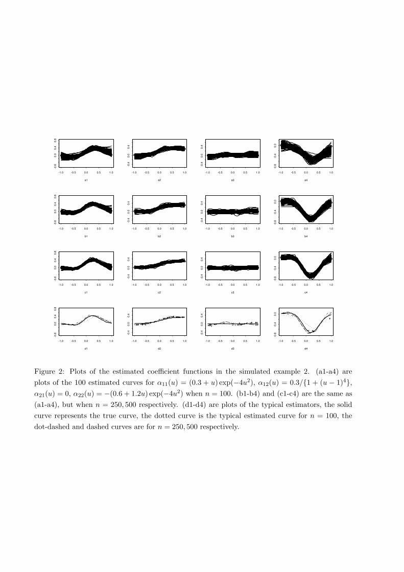
l=1,2 . Theresults are also graphically presented in Figure 2. Similar to Example 1, the estimation improves assample size increases, supporting the asymptotic result (Theorem 1). The model selection resultsare presented in Table 2, indexed as ‘Example 2’. As Example 1, AIC tends to overfit comparedwith BIC, and for n = 250, 500, the model selection result is satisfactory.
(Insert Table 3 about here)
(Insert Figure 2 about here)
4.3 West German real GNP
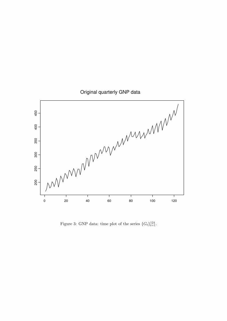
Now, we compare the estimation and prediction performances of the polynomial spline and marginalintegration methods through the West German real GNP. For other empirical examples, see Xue& Yang (2005b). The data consists of the quarterly West German real GNP from January 1960 toDecember 1990, denote as {Gt}124
t=1, where Gt is the real GNP in the t-th quarter (the first quarterbeing from January 1, 1960 to April 1, 1960). From its time plot (Figure 3), {Gt}124
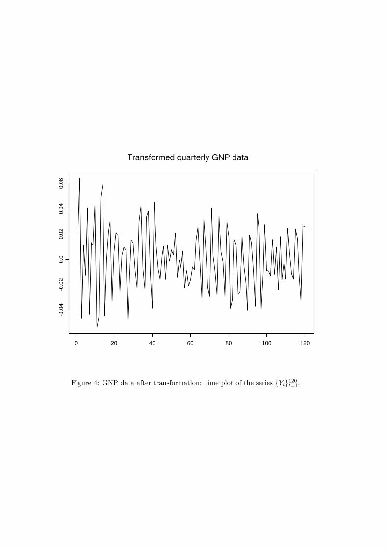
t=1 appears tohave both trend and seasonality. After removing the seasonal means from {log (Gt+4/Gt+3)}120
t=1,we obtain a more stationary time series denoted as {Yt}120
t=1, whose time plot is given in Figure 4.As the nonparametric alternative to the linear autoregressive model selected by BIC
Yt = a1Yt−2 + a2Yt−4 + σεt, (4.1)
Xue & Yang (2005a) proposed the additive coefficient model
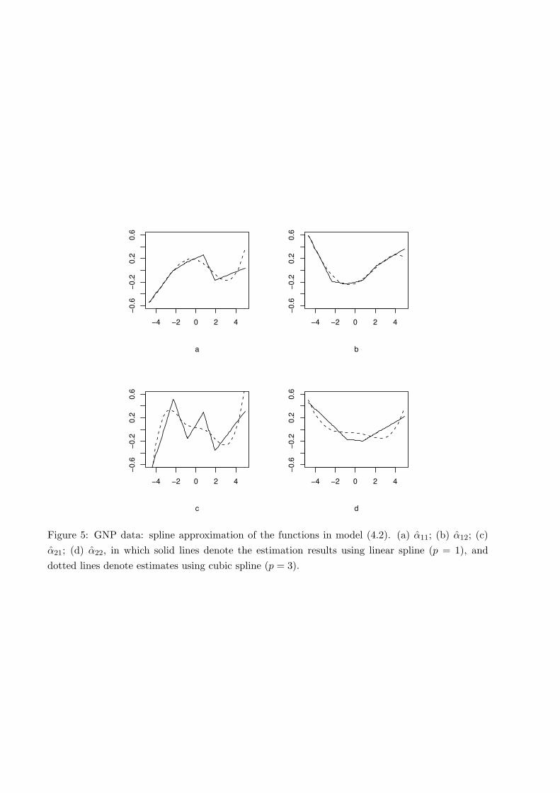
Yt = {c1 + α11 (Yt−1) + α12 (Yt−8)}Yt−2 + {c2 + α21 (Yt−1) + α22 (Yt−8)}Yt−4 + σεt, (4.2)
which is fitted by linear and cubic splines (p = 1, 3). Following Xue & Yang (2005a), we use the first110 observations for estimation and the last 10 observations for one-step prediction. Table 4 givesthe averaged squared estimation errors (ASE) and averaged squared prediction errors (ASPE)of different fittings. Polynomial spline is better than the marginal integration method overall,while model (4.2) significantly improves over model (4.1) in both estimation and prediction. Forvisualization, plots of the function estimates are given in Figure 5.
(Insert Table 4 about here)
(Insert Figure 3 about here)
(Insert Figure 4 about here)
(Insert Figure 5 about here)
5. Conclusion
A polynomial spline estimation method together with a BIC model selection procedure have beenproposed for the semiparametric additive coefficient model. Consistency has been established underbroad geometric mixing assumptions. The procedures apply to nonlinear regression with weaklydependence as well as i.i.d. observations. Implementation of the proposed method is as easy and
9
fast as linear regression, with excellent performance as Theorem 1 stipulates. Empirical studyillustrates that these methods are very useful for statistical inference in multivariate regressionsetting.
Acknowledgements
The paper is substantially improved thanks to the helpful comments of Editor Jane-Ling Wang,an associate editor and the referees. Research has been supported in part by National ScienceFoundation grants BCS 0308420, DMS 0405330, and SES 0127722.
References
Bosq, D. (1998). Nonparametric Statistics for Stochastic Processes: estimation and prediction,2nd Ed. Springer-Verlag, New York.
Cai, Z., Fan, J. and Yao, Q. W. (2000). Functional-coefficient regression models for nonlineartime series. J. Amer. Statist. Assoc. 95, 941-956.
Chen, R. and Tsay, R. S. (1993a). Nonlinear additive ARX models. J. Amer. Statist. Assoc. 88,955-967.
Chen, R. and Tsay, R. S. (1993b). Functional-coefficient autoregressive models. J. Amer. Statist.Assoc. 88, 298-308.
de Boor, C. (2001). A Practical Guide to Splines. Springer, New York.
Devore R. A. and Lorentz, G. G. (1993). Constructive Approximation. Springer-Varlag, BerlinHeidelberg.
Hastie, T. J. and Tibshirani, R. J. (1990). Generalized Additive Models. Chapman and Hall,London.
Hastie, T. J. and Tibshirani, R. J. (1993). Varying-coefficient models. J. Roy. Statist. Soc. Ser.B 55, 757-796.
Huang, J. Z. (1998a). Projection estimation in multiple regression with application to functionalANOVA models. Ann. Statist. 26, 242-272.
Huang, J. Z. (1998b). Functional ANOVA models for generalized regression. J. Multivariate Anal.67, 49-71.
Huang, J. Z. and Shen, H. (2004). Functional coefficient regression models for non-linear timeseries: a polynomial spline approach. Scandinavian Journal of Statistics 31, 515-534.
Huang, J. Z., Wu, C. O. and Zhou, L. (2002). Varying-coefficient models and basis functionapproximations for the analysis of repeated measurements. Biometrika 89, 111-128.
10
Huang, J. Z., and Yang, L. (2004). Identification of nonlinear additive autoregressive models.Journal of the Royal Statistical Society Series B 66, 463-477.
Stone, C. J. (1985). Additive regression and other nonparametric models. Ann. Statist. 13, 689- 705.
Xue, L. and Yang, L. (2005a). Estimation of semiparametric additive coefficient model. Journalof Statistical Planning and Inference in press.
Xue, L. and Yang, L. (2005b). Additive coefficient modeling via polynomial spline, downloadableat http://www.msu.edu/˜yangli/addsplinefull.pdf.
Department of Statistics and Probability, Michigan State University, East Lansing, MI 48824, USA
E-mail: [email protected]
Department of Statistics and Probability, Michigan State University, East Lansing, MI 48824, USA
E-mail: [email protected]
Appendix
A.1 Assumptions and notations
The following assumptions are needed for our theoretical results.
(C1) The tuning variables X = (X1, . . . , Xd2) are compactly supported and without lose of general-ity, we assume that its support is χ = [0, 1]d2. The joint density of X, denoted by f(x), is ab-solutely continuous and bounded away from zero and infinity, that is, 0 < c1 ≤ minx∈χ f(x) ≤maxx∈χ f(x) ≤ c2 < ∞.
(C2) (i) There exist positive constants 0 < c3 ≤ c4, such that c3Id1 ≤ E(TTT |X = x) ≤c4Id1 forall x ∈ χ. Here Id1denotes the d1 × d1 identity matrix. There also exist positive constantsc5, c6 such that, c5 ≤ E
{(TlTl′
)2+δ0 |X = x}≤ c6 a.s. for some δ0 > 0 and l, l
′= 1, . . . , d1.
(ii) For some sufficient large m > 0, E |Tl|m < +∞, for l = 1, . . . , d1.
(C3) The d2 sets of knots denoted as ks,n = {0 = xs,0 ≤ xs,1 ≤ · · · ≤ xs,Nn ≤ xs,Nn+1 = 1} , s =1, . . . , d2, are quasi-uniform, that is, there exists c7 > 0
maxs=1,...,d2
max (xs,j+1 − xs,j , j = 0, . . . , Nn)min(xs,j+1 − xs,j , j = 0, . . . , Nn)
≤ c7.
The number of interior knots Nn ³ n1
2p+3 , where p is the degree of the spline and ‘ ³′meaningboth sides have the same order. In particular, h ³ n
− 12p+3 .
(C4) The vector process {ςt}∞t=−∞ = {(Yt,Xt,Tt)}∞t=−∞ is strictly stationary and geometriclystrongly mixing, that is, its α -mixing coefficient α(k) ≤ cρk, for constants c > 0, 0 < ρ < 1,where α(k) = supA∈σ(ςt,t≤0),B∈σ(ςt,t≥k) |P (A)P (B)− P (AB)| .
11
(C5) The conditional variance function σ2 (x, t) is measurable and bounded.
Assumptions (C1)-(C5) are common in the nonparametric regression literature. Assumption(C1) is the same as Condition 1, p.693 of Stone (1985), assumption (c), p.468 of Huang & Yang(2004). Assumption (C2) (i) is a direct extension of condition (ii), p.531 of Huang & Shen (2004).Assumption (C2) (ii) is a direct extension of condition (v), p.531 of Huang & Shen (2004), and ofthe moment condition A.2 (c) p.952 of Cai, Fan & Yao (2000). Assumption (C3) is the same as inequation (6), p.249 of Huang (1998a), and also p.59, Huang (1998b). Assumption (C4) is similarto condition (iv), p.531 of Huang & Shen (2004). Assumption (C5) is the same as p.242 of Huang(1998a), and p.465 of Huang & Yang (2004).
In this Appendix, whenever proofs are brief, see Xue & Yang (2005b) for details.
A.2 Technical lemmas
For notational convenience, we introduce, for 1 ≤ l ≤ d1, 1 ≤ s ≤ d2,
αl0 = cl0 +d2∑
s=1
Eα∗ls, αls(xs) = α∗ls(xs)− Eα∗ls. (A.1)
Then one can rewrite m (3.1) as m =∑d1
l=1
{αl0 +
∑d2s=1 αls(xs)
}tl, with {αls(xs)}1≤l≤d1
∈ ϕ0s.
The terms in (A.1) are not directly observable and serve only as the intermediate step in the proofof Theorem 1. By observing that, for 1 ≤ l ≤ d1, 1 ≤ s ≤ d2,
αl0 = αl0 −d2∑
s=1
Enαls, αls(xs) = αls(xs)− Enαls, (A.2)
the terms {αl0}d1l=1 , {αls(xs)}d1,d2
l=1,s=1 and {αl0}d1l=1 , {αls(xs)}d1,d2
l=1,s=1 differ only by a constant. Insection A.3, we first prove the consistency of {αl0}d1
l=1 , {αls(xs)}d1,d2
l=1,s=1 in Theorem 3. Then Theorem1 follows by showing {Enαls}d1,d2
s=1,l=1 are negligible.B-spline basis is used in the proofs, which is equivalent to the truncated power basis used in
implementation, but has nice local properties (de Boor 2001). With Jn = Nn + p, we denote theB-spline basis of ϕs by bs = {bs,0, . . . , bs,Jn}. For 1 ≤ s ≤ d2, denote Bs = {Bs,1, . . . , Bs,Jn} with
Bs,j =√
Nn
(bs,j − E (bs,j)
E (bs,0)bs,0
), j = 1, . . . , Jn. (A.3)
Note that assumption (C1) ensures all Bs,j ’s are well defined.Now, let B = (1,B1,1, . . . , B1,Jn , . . . , Bd2,1, . . . , Bd2,Jn)T with 1 being the identity function de-
fined on χ. Define G = (Bt1, . . . ,Btd1)T = (G1, . . . , GRn)T ,with Rn = d1 (d2Jn + 1). Then G is
a set of basis of Mn. By (3.1), one has m (x, t) =∑d1
l=1
{c∗l0 +
∑d2s=1
Jn∑j=1
c∗ls,jBs,j (xs)
}tl, in which
{c∗l0, c
∗ls,j , 1 ≤ l ≤ d1, 1 ≤ s ≤ d2, 1 ≤ j ≤ Jn
}minimize the sum of squares as in (3.3), with ws,j
replaced by Bs,j . Then Lemma 1 leads to αl0 = c∗l0, αls =Jn∑j=1
c∗ls,jBs,j (xs) , 1 ≤ l ≤ d1, 1 ≤ s ≤ d2.
12
Theorem 3 Under assumptions (C1)-(C5), if αls ∈ Cp+1 ([0, 1]) , for 1 ≤ l ≤ d1, 1 ≤ s ≤ d2, onehas
‖m−m‖2 = Op
(hp+1 +
√1/nh
),
max1≤l≤d1
|αl0 − αl0|+ max1≤l≤d1,1≤s≤d2
‖αls − αls‖2 = Op
(hp+1 +
√1/nh
).
To prove Theorem 3, we first present the properties of the basis G in Lemmas A.1-A.3.
Lemma A.1 For any 1 ≤ s ≤ d2, and spline basis Bs,j as in (A.3), one has
(i) E (Bs,j) = 0, E |Bs,j |k ³ Nk/2−1n , for k > 1, j = 1, . . . , Jn.
(ii) There exists a constant C > 0 such that for any vector a = (a1, . . . , aJn)T , as n → ∞,∥∥∥∥∥Jn∑j=1
ajBs,j
∥∥∥∥∥2
2
≥ CJn∑j=1
a2j .
Proof. (i) follows from Theorem 5.4.2 of DeVore & Lorentz (1993), and assumptions (C1), (C3).To prove (ii), we introduce the auxiliary knots xs,−p = . . . = xs,−1 = xs,0 = 0, and xs,Nn+p+1 =. . . = xs,Nn+2 = xs,Nn+1 = 1 for the knots ks. Then
∥∥∥∥∥∥
Jn∑
j=1
ajBs,j
∥∥∥∥∥∥
2
2
≥ c1
∥∥∥∥∥∥
Jn∑
j=1
ajBs,j
∥∥∥∥∥∥
∗2
2
= c1
∥∥∥∥∥∥
Jn∑
j=1
aj
√Nnbs,j −
Jn∑
j=1
aj
√NnE (bs,j)E (bs,0)
bs,0
∥∥∥∥∥∥
∗2
2
,
where ‖·‖∗2 is defined as ‖f‖∗2 =√∫
f2 (x) dx, for any square integrable function f . Let ds,j =(xs,j+1 − xs,j−p) / (p + 1). Then Theorem 5.4.2 of Devore & Lorentz (1993) ensures that for aC > 0, the above is
≥ c1C
Jn∑
j=1
a2jNnds,j +
Jn∑
j=1
aj
√NnE (bs,j)E (bs,0)
2
ds,0
≥ c1C
Jn∑
j=1
a2jNnds,j ≥ c1C (p + 1) /c7
Jn∑
j=1
a2j . ¥
Lemma A.2 There exists a constant C > 0, such that as n → ∞, for any sets of coefficients,{cl0, cls,j , l = 1, . . . , d1; s = 1, . . . , d2; j = 1, . . . , Jn}
∥∥∥∥∥∥
d1∑
l=1
cl0 +
d2∑
s=1
Jn∑
j=1
cls,jBs,j
tl
∥∥∥∥∥∥
2
2
≥ C
d1∑
l=1
c2
l0 +d2∑
s=1
Jn∑
j=1
c2ls,j
.
Proof. The result follows immediately from Lemmas 1, and A.1. ¥
Lemma A.3 Let 〈G,G〉 be the Rn×Rn matrix defined as 〈G,G〉 = (〈Gi,Gj〉)Rn
i,j=1. Define 〈G,G〉nsimilarly as 〈G,G〉 , but replace the theoretical inner product with the empirical inner product, andlet D = diag(〈G,G〉). Define Qn = sup
∣∣D−1/2 (〈G,G〉n − 〈G,G〉)D−1/2∣∣, where sup is taken
oven all the elements in the random matrix. Then as n →∞, Qn = Op
(√n−1h−1 log2(n)
).
13

Proof. For notation simplicity, we consider the diagonal terms. For any 1 ≤ l ≤ d2, 1 ≤ s ≤d1, 1 ≤ j ≤ Jn fixed, let ξ = (En − E)
{B2
s,j (Xs) T 2l
}= 1
n
n∑i=1
ξi, in which ξi = B2s,j (Xis) T 2
il −
E{
B2s,j (Xis) T 2
il
}. Define Til = TilI{|Til|≤nδ}, for some 0 < δ < 1, and define ξ, ξi similarly as ξ
and ξi, but replace Tl with Tl′ . Then for any ε > 0, one has
P
(|ξ| ≥ ε
√log2(n)/ (nh)
)≤ P
(∣∣∣ξ∣∣∣ ≥ ε
√log2(n)/ (nh)
)+ P (ξ 6= ξ), (A.4)
in which P (ξ 6= ξ) ≤ P(Til 6= Til, for some i = 1, . . . , n
)≤
n∑i=1
P(|Til| ≥ nδ
) ≤ E |Tl|m /nmδ−1.
Also note that sup0≤xs≤1 |Bs,j (xs)| = sup0≤xs≤1
∣∣√Nn {bs,j − E (bs,j) bs,0/E (bs,0)}∣∣ ≤ c
√Nn, for
some c > 0. Then by Minkowski’s inequality, for any positive integer k ≥ 3
E∣∣∣ξi
∣∣∣k≤ 2k−1
[E
∣∣∣B2s,j (Xs) T 2
l
∣∣∣k
+{
E∣∣∣B2
s,j (Xs) T 2l
∣∣∣}k
]≤ 2k−1
[n2δkckNk
n + (cNn)k]≤ n2δkckNk
n .
On the other hand
E∣∣∣ξi
∣∣∣2≥ E
∣∣B2s,j (Xs) T 2
l
∣∣2 /2− E2{B2
s,j (Xs) T 2l
}− E∣∣∣B2
s,j (Xs) T 2l I{|Tl|>nδ}
∣∣∣2/2,
in which, under assumption (C2)
E∣∣∣B2
s,j (Xs) T 2l I{|Tl|>nδ}
∣∣∣2≤ E
∣∣∣B4s,j (Xs) E
(T 4+δ0
l /nδδ0 |X)∣∣∣ ≤ c6E
∣∣B4s,j (Xs)
∣∣ /nδδ0 ≤ cNn/nδδ0 ,
where δ0 is as in assumption (C2). Furthermore
E2{B2
s,j (Xs) T 2l
} ≤ c24E
2{B2
s,j (Xs)} ≤ c,
E∣∣B2
s,j (Xs) T 2l
∣∣2 ≥ c5E |Bs,j (Xs)|4 ≥ c1c5
∫|Bs,j (xs)|4 dxs ≥ cc1c5Nn.
Thus E∣∣∣ξi
∣∣∣2≥ cNn − c− cNn
nδδ0≥ cNn. So there exists a constant c > 0, such that for all ≥ 3
E∣∣∣ξi
∣∣∣k≤ n2δkckNk
n ≤(cn6δN2
n
)k−2k!E
∣∣∣ξi
∣∣∣2.
Then one can apply Theorem 1.4 of Bosq (1998) to∑n
i=1 ξi, with the Cramer’s constant cr =cn6δN2
n. That is, for any ε > 0, q ∈ [1, n
2
], and k ≥ 3, one has
P
1
n
∣∣∣∑n
i=1ξi
∣∣∣ ≥ ε
√log2(n)
nh
≤ a1 exp
− qε2 log2(n)
nh
25m22 + 5εcr
√log2(n)
nh
+ a2(k)α
([n
q + 1
]) 2k2k+1
,
where
a1 = 2n
q+ 2
1 +
ε2 log2(n)nh
25m22 + 5εcr
√log2(n)
nh
, a2(k) = 11n
1 +
5mk
2k+1p
ε
√log2(n)
nh
,m2
2 = Eξ2i ,mp =
∥∥∥ξi
∥∥∥p.
14
Observe that 5εcr
√log2(n)
nh = 5εcn6δN2n
√log2(n)
nh = o(1), by taking δ < 2p12(2p+3) . Then by taking
q = n/ {c0 log (n)} , one has a1 = O(
nq
)= O {log(n)} , a2(k) = O
(n N
k2k+1
n√log2(n)
nh
)= o
(n
32
). Thus,
for n large enough
P
(1n
∣∣∣∑n
i=1ξi
∣∣∣ ≥ ε
√log2(n)/ (nh)
)≤ c log(n) exp
{−ε2 log(n)
50c0m22
}+ cn
32 exp {− log(ρ)c0 log (n)} .
Thus by (A.4), taking c0, ε, m large enough and use assumption (C4), one has that
∑∞n=1
P
(sup |〈G,G〉n − 〈G,G〉| ≥ ε
√log2(n)/ (nh)
)
≤∑∞
n=1{d1d2(Nn + 2)}2
{c log(n) exp
{−ε2 log(n)
25c0
}+ cn
32 exp {− log(ρ)c0 log (n)}+
E |Tl|mnmδ−1
}
<∑∞
n=1{d1d2(Nn + 2)}2 n−3 < +∞,
in which Nn ³ n1
2p+3 . Then the lemma follows from Borel-Cantelli Lemma and Lemma A.1. ¥
Lemma A.4 As n →∞, one has
supφ1∈Mn,φ2∈Mn
∣∣∣∣〈φ1, φ2〉n − 〈φ1, φ2〉
‖φ1‖2 ‖φ2‖2
∣∣∣∣ = Op
√log2(n)
nh
.
In particular, there exist constants 0 < c < 1 < C such that, except on an event whose probabilitytends to zero as n →∞, c ‖m‖2 ≤ ‖m‖2,n ≤ C ‖m‖2 ,∀m ∈Mn.
Proof. With vector notation, one can write φ1 = aT1 G, φ2 = aT
2 G, for Rn × 1 vectors a1,a2.
|〈φ1, φ2〉n − 〈φ1, φ2〉| =Rn∑
i,j=1
|a1ia2j |∣∣〈Gi, Gj〉n − 〈Gi, Gj〉
∣∣
≤ Qn
Rn∑
i,j=1
|a1ia2j | ‖Gi‖2 ‖Gj‖2 ≤ QnC
Rn∑
i,j=1
|a1ia2j | ≤ QnC√
aT1 a1aT
2 a2.
On the other hand by Lemma A.2,
‖φ1‖22 ‖φ2‖2
2 =(aT
1 〈G,G〉a1
) (aT
2 〈G,G〉a2
) ≥ C2aT1 a1aT
2 a2.
Then
∣∣∣∣〈φ1, φ2〉n − 〈φ1, φ2〉
‖φ1‖2 ‖φ2‖2
∣∣∣∣ ≤∣∣∣∣∣∣QnC
√aT
1 a√
aT2 a2
C√
aT1 a1
√aT
2 a2
∣∣∣∣∣∣= Op (Qn) = Op
√log2(n)
nh
. ¥
Lemma A.4 shows that the empirical and theoretical inner products are uniformly close over theapproximation space Mn. This lemma plays the crucial role analogous to that of Lemma 10 inHuang (1998a). Our result is new in that (i) the spline basis of Huang (1998a) must be bounded,
15
whereas the term t in basis G makes it possibly bounded; (ii) Huang (1998a)’s setting is i.i.d. withuniform approximation rate of op (1), while our setting is α-mixing, broadly applicable to time
series data, with approximation rate the sharper Op
(√log2(n)/nh
). The next lemma follows
immediately from Lemmas A.2 and A.4.
Lemma A.5 There exists constant C > 0 such that except on an event whose probability tends tozero as n →∞
∥∥∥∥∥∥
d1∑
l=1
cl0 +
d2∑
s=1
Jn∑
j=1
cls,jBs,j
tl
∥∥∥∥∥∥
2
2,n
≥ C
d1∑
l=1
c2
l0 +d2∑
s=1
Jn∑
j=1
c2ls,j
.
A.3 Proof of mean square consistency
Proof of Theorem 3. We denote
Y =(Y1, . . . , Yn)T ,m = {m(X1,T1), . . . , m(Xn,Tn)}T ,E = {σ(X1,T1)ε1, . . . , σ(Xn,Tn)εn}T .
Note that Y = m + E, and projecting it onto Mn, one has m = m+ e, where m is defined in (3.1),and m, e are the solution to (3.1) with Yi replaced by m(Xi,Ti) and σ(Xi,Ti)εi respectively. Alsoone can uniquely represent m as m =
∑d1l=1
(αl0 +
∑d2s=1 αls
)tl, αls ∈ ϕ0
s. With these notations,one has the error decomposition m − m = m − m + e, where m − m is the bias term, and e isthe variance term. Since for 1 ≤ l ≤ d1, 1 ≤ s ≤ d2, αls ∈ Cp+1 ([0, 1]) , by Lemma 2, thereexist C > 0 and spline functions gls ∈ ϕ0
s, such that ‖αls − gls‖∞ ≤ Chp+1. Let mn (x, t) =∑d1l=1
{αl0 +
∑d2s=1 gls (xs)
}tl ∈Mn. One has
‖m−mn‖2 ≤d1∑
l=1
d2∑
s=1
‖{αls − gls} tl‖2 ≤ c4
d1∑
l=1
d2∑
s=1
‖αls − gls‖∞ ≤ c4Chp+1. (A.5)
Also ‖m−mn‖2,n ≤ Chp+1 a.s. Then by the definition of projection, one has
‖m−m‖2,n ≤ ‖m−mn‖2,n ≤ Chp+1,
which also implies ‖m−mn‖2,n ≤ ‖m−m‖2,n + ‖m−mn‖2,n ≤ Chp+1. By Lemma A.4
‖m−mn‖2 ≤ ‖m−mn‖2,n (1−Qn)1/2 = Op
(hp+1
).
Together with (A.5), one has‖m−m‖2 = Op
(hp+1
). (A.6)
Next we consider the variance term e. For some set of coefficients a = (a1, . . . , aRn)T ,
one can write e (x, t)=∑Rn
j=1 ajGj (x, t) . Denote N = [N (G1) , . . . , N (GRn)]T , with N (Gj) =1n
∑ni=1 Gj (Xi,Ti) σ (Xi,Ti) εi. By the definition of projection, one has
(〈Gj , Gj〉n)Rn
j,j′=1a = N.
16
Multiplying both sides with the same vector, one gets aT(〈Gj , Gj〉n
)Rn
j,j′=1a = aTN. Now, by
Lemmas A.2, A.4, the LHS is∥∥∥∑Rn
j=1 ajGj
∥∥∥2
2,n≥ C (1−Qn)
∑Rnj=1 a2
j , while the RHS is
≤
Rn∑
j=1
a2j
1/2
Rn∑
j=1
(1n
n∑
i=1
Gj (Xi,Ti) σ (Xi,Ti) εi
)2
1/2
.
Hence C (1−Qn)∑Rn
j=1 a2j ≤
(∑Rnj=1 a2
j
)1/2 {∑Rnj=1
(1n
∑ni=1 Gj (Xi,Ti) σ (Xi,Ti) εi
)2}1/2
entail-ing
Rn∑
j=1
a2j
1/2
≤ C−1 (1−Qn)−1
Rn∑
j=1
(1n
n∑
i=1
Gj (Xi,Ti) σ (Xi,Ti) εi
)2
1/2
,
and as a result ‖e‖22 ≤ C (1−Qn)−2
{∑Rnj=1
(1n
∑ni=1 Gj (Xi,Ti) σ (Xi,Ti) εi
)2}
. Since εi is inde-pendent of {(Xj ,Tj) , j ≤ i} , for i = 1, . . . , n, one has
Rn∑
j=1
E
(1n
n∑
i=1
Gj (Xi,Ti) σ (Xi,Ti) εi
)2
=Rn∑
j=1
1n
E {Gj (Xi,Ti) σ (Xi,Ti) εi}2 ≤ CJn
n= O
(1
nh
),
by assumptions (C2), (C5) and Lemma A.1 (i). Therefore ‖e‖22 = Op
(n−1h−1
). This, together with
(A.6) prove ‖m−m‖2 = Op
(hp+1 +
√1/nh
). The second part of Theorem 3 follows from Lemma
1, which entails that for C > 0, ‖m−m‖22 ≥ C
[∑d1l=1
{(αl0 − αl0)
2 +∑d2
s=1 ‖αls − αls‖22
}]. ¥
Proof of Theorem 1. By (A.2), one only needs to show |Enαls| = Op
(hp+1 +
√1/nh
), for
1 ≤ l ≤ d1, 1 ≤ s ≤ d2. Note that |Enαls| ≤ |En {αls − αls}|+ |Enαls| , whose first term
|En {αls − αls}| ≤ ‖αls − αls‖2,n ≤ ‖αls − αls‖2,n + ‖αls − αls‖2,n
≤ ‖αls − gls‖2,n + ‖αls − gls‖2,n + ‖αls − αls‖2,n ,
with ‖αls − gls‖2,n ≤ ‖αls − gls‖∞ ≤ Chp+1, and applying Lemmas 1 and A.3, one has
‖αls − gls‖2,n ≤ (1 + Qn) ‖αls − gls‖2 ≤ (1 + Qn) ‖m−mn‖2 = Op
(hp+1
),
‖αls − αls‖2,n ≤ (1 + Qn) ‖αls − αls‖2,n ≤ (1 + Qn) ‖e‖2 = Op
(√1/nh
).
Thus |En {αls − αls}| = Op
(hp+1 +
√1/nh
). Since |Enαls| = Op (1/
√n), one now has |Enαls| =
Op
(hp+1 +
√1/nh
). Theorem 1 now follows from the triangular inequality. ¥
A.4 Proof of BIC consistency
We denote the model space MS and the approximation space Mn,S of mS separately as
MS =
m (x, t) =
d1∑
l=1
αl (x) tl; αl (x) = αl0 +∑
s∈Sl
αls(xs);αls ∈ H0s
,
Mn,S =
mn (x, t) =
d1∑
l=1
gl (x) tl; gl (x) = αl0 +∑
s∈Sl
gls(xs); gls ∈ ϕ0s
.
17
If S ⊂ Sf , MS ⊂ MSfand Mn,S ⊂ Mn,Sf
. Let ProjS (Projn,S) be the orthogonal least squareprojector onto MS (Mn,S) with respect to the empirical inner product. Then mS (3.7) can beviewed as: mS = Projn,S (Y). As a special case of Theorem 1, one has the following result.
Lemma A.6 Under the same conditions as in Theorem 1, one has
‖mS −mS‖2 = Op
(1/Np+1
S +√
NS/n)
.
Now denote c (S,m) = ‖ProjS m−m‖2. One has if m ∈MS0 , ProjS0m = m, thus c (S0,m) =
0; and if S overfits, since m ∈MS0 ⊂MS , c (S,m) = 0; and if S underfits, c (S,m) > 0.
Proof of Theorem 2. Notice that
BICS − BICS0 =MSES −MSES0
MSES0
{1 + op (1)}+qS − qS0
nlog (n)
=MSES −MSES0
E{σ2 (X,T)}(1 + op(1)){1 + op (1)}+ n
− 2p+22p+3 log (n) ,
since qS − qS0 ³ n1/(2p+3), and
MSEs0 ≤1n
n∑
i=1
{Yi −m (Xi,Ti)}2+1n
n∑
i=1
{mS0 (Xi,Ti)−m (Xi,Ti)}2 = E{σ2 (X,T)}(1+op(1)).
Case 1 (Overfitting): Suppose that S0 ⊂ S and S0 6= S. One has
MSEs −MSEs0 = ‖ms − ms,0‖22,n = ‖ms − ms,0‖2
2 {1 + op (1)}≤
(‖ms −m‖2
2 + ‖ms,0 −m‖22
){1 + op (1)} = Op
(n−(2p+2)/(2p+3)
).
Thus limn→+∞ {P (BICs − BICs0 > 0)} = 1. To see why the assumption qS − qS0 ³ n1/(2p+3) isnecessary, suppose qS0 ³ nr, with r > 1/(2p + 3) instead. Then it can be shown that
MSEs −MSEs0 = − nr−1
E{σ2 (X,T)} {1 + op (1)} − nr−1 log(n) {1 + op(1)} ,
which leads to limn→+∞ {P (BICs − BICs0 < 0)} = 1, instead.Case 2 (Underfitting): Similarly as in Huang & Yang (2004), we can show that if S underfits,
MSES −MSES0 ≥ c2 (S,m) + op (1) . Then
BICS − BICS0 ≥c2 (S,m) + op (1)
E{σ2 (X,T)}(1 + op(1))+ op (1) ,
which implies that limn→+∞ {P (BICs − BICs0 > 0)} = 1. ¥
18
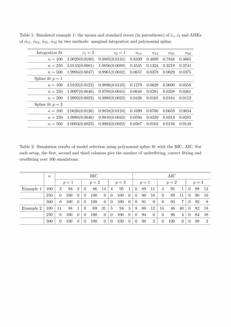
Table 1: Simulated example 1: the means and standard errors (in parentheses) of c1, c2 and AISEsof α11, α12, α21, α22 by two methods: marginal integration and polynomial spline.
Integration fit c1 = 2 c2 = 1 α11 α12 α21 α22
n = 100 2.0029(0.0180) 0.9805(0.0134) 0.8339 0.4699 0.7948 0.4665
n = 250 2.0143(0.0081) 1.0056(0.0089) 0.4545 0.1324 0.3219 0.3741
n = 500 1.9994(0.0047) 0.9961(0.0042) 0.0657 0.0378 0.0629 0.0375
Spline fit p = 1
n = 100 2.0102(0.0122) 0.9896(0.0123) 0.1279 0.0629 0.0690 0.0558
n = 250 1.9997(0.0046) 0.9795(0.0044) 0.0648 0.0291 0.0328 0.0261
n = 500 1.9992(0.0023) 0.9988(0.0022) 0.0438 0.0165 0.0164 0.0152
Spline fit p = 3
n = 100 2.0026(0.0126) 0.9858(0.0124) 0.1699 0.0700 0.0659 0.0634
n = 250 1.9988(0.0046) 0.9810(0.0043) 0.0594 0.0320 0.0313 0.0285
n = 500 2.0003(0.0023) 0.9982(0.0022) 0.0387 0.0162 0.0156 0.0149
Table 2: Simulation results of model selection using polynomial spline fit with the BIC, AIC. Foreach setup, the first, second and third columns give the number of underfitting, correct fitting andoverfitting over 100 simulations.
n BIC AICp = 1 p = 2 p = 3 p = 1 p = 2 p = 3
Example 1 100 3 94 3 0 86 14 4 95 1 0 89 11 4 95 1 0 88 12
250 0 100 0 0 100 0 0 100 0 0 90 10 0 89 11 0 90 10
500 0 100 0 0 100 0 0 100 0 0 91 9 0 93 7 0 92 8
Example 2 100 11 88 1 0 69 31 5 94 5 8 80 12 14 46 40 0 82 18
250 0 100 0 0 100 0 0 100 0 0 94 6 0 96 4 0 84 16
500 0 100 0 0 100 0 0 100 0 0 98 2 0 100 0 0 98 2
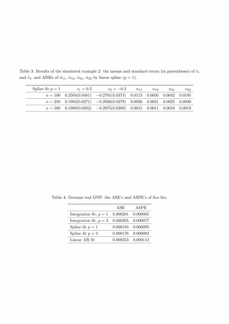
Table 3: Results of the simulated example 2: the means and standard errors (in parentheses) of c1
and c2, and AISEs of α11, α12, α21, α22 by linear spline (p = 1).
Spline fit p = 1 c1 = 0.2 c2 = −0.3 α11 α12 α21 α22
n = 100 0.2504(0.0481) −0.2701(0.0374) 0.0113 0.0050 0.0042 0.0195
n = 250 0.1983(0.0271) −0.2936(0.0279) 0.0030 0.0021 0.0025 0.0039
n = 500 0.1989(0.0202) −0.2975(0.0209) 0.0015 0.0011 0.0016 0.0019
Table 4: German real GNP: the ASE’s and ASPE’s of five fits.
ASE ASPE
Integration fit, p = 1 0.000201 0.000085
Integration fit, p = 3 0.000205 0.000077
Spline fit p = 1 0.000183 0.000095
Spline fit p = 3 0.000176 0.000082
Linear AR fit 0.000253 0.000112
−3 −1 1 2 3
−20
2
a1
−3 −1 1 2 3
−30
3
a2
−3 −1 1 2 3
−21
a3
−3 −1 1 2 3
−20
2
a4
−3 −1 1 2 3
−20
2
b1
−3 −1 1 2 3
−30
3
b2
−3 −1 1 2 3
−21
b3
−3 −1 1 2 3
−20
2
b4
−3 −1 1 2 3
−20
2
c1
−3 −1 1 2 3
−30
3
c2
−3 −1 1 2 3
−21
c3
−3 −1 1 2 3−2
02
c4
−3 −1 1 2 3
−20
2
d1
−3 −1 1 2 3
−30
3
d2
−3 −1 1 2 3
−21
d3
−3 −1 1 2 3
−20
2
d4
Figure 1: Plots of the estimated coefficient functions in the simulated example 1. (a1-a4) areplots of the 100 estimated curves for α11(x) = sin(2(4x − 2)) + 2 exp(−2(x − 0.5)2), α12(x) = x,α21(x) = sin(x), α22(x) = 0, for n = 100. (b1-b4) and (c1-c4) are the same as (a1-a4), but forn = 250 and n = 500 respectively. (d1-d4) are plots of the typical estimators, the solid curverepresents the true curve, the dotted curve is the typical estimated curve for n = 100, the dot-dashed and dashed curves are for n = 250, 500 respectively.
-1.0 -0.5 0.0 0.5 1.0
-0.6
0.0
0.4
0.8
a1
-1.0 -0.5 0.0 0.5 1.0
-0.4
0.0
0.4
a2
-1.0 -0.5 0.0 0.5 1.0
-0.4
0.0
0.4
a3
-1.0 -0.5 0.0 0.5 1.0
-0.8
-0.4
0.0
a4
-1.0 -0.5 0.0 0.5 1.0
-0.6
0.0
0.4
0.8
b1
-1.0 -0.5 0.0 0.5 1.0
-0.4
0.0
0.4
b2
-1.0 -0.5 0.0 0.5 1.0
-0.4
0.0
0.4
b3
-1.0 -0.5 0.0 0.5 1.0
-0.8
-0.4
0.0
b4
-1.0 -0.5 0.0 0.5 1.0
-0.6
0.0
0.4
0.8
c1
-1.0 -0.5 0.0 0.5 1.0
-0.4
0.0
0.4
c2
-1.0 -0.5 0.0 0.5 1.0
-0.4
0.0
0.4
c3
-1.0 -0.5 0.0 0.5 1.0
-0.8
-0.4
0.0
c4
-1.0 -0.5 0.0 0.5 1.0
-0.6
0.0
0.4
0.8
d1
-1.0 -0.5 0.0 0.5 1.0
-0.4
0.0
0.4
d2
-1.0 -0.5 0.0 0.5 1.0
-0.4
0.0
0.4
d3
-1.0 -0.5 0.0 0.5 1.0
-0.8
-0.4
0.0
d4
Figure 2: Plots of the estimated coefficient functions in the simulated example 2. (a1-a4) areplots of the 100 estimated curves for α11(u) = (0.3 + u) exp(−4u2), α12(u) = 0.3/{1 + (u − 1)4},α21(u) = 0, α22(u) = −(0.6 + 1.2u) exp(−4u2) when n = 100. (b1-b4) and (c1-c4) are the same as(a1-a4), but when n = 250, 500 respectively. (d1-d4) are plots of the typical estimators, the solidcurve represents the true curve, the dotted curve is the typical estimated curve for n = 100, thedot-dashed and dashed curves are for n = 250, 500 respectively.
0 20 40 60 80 100 120
200
250
300
350
400
450
Original quarterly GNP data
Figure 3: GNP data: time plot of the series {Gt}124t=1.
0 20 40 60 80 100 120
-0.0
4-0
.02
0.0
0.02
0.04
0.06
Transformed quarterly GNP data
Figure 4: GNP data after transformation: time plot of the series {Yt}120t=1.
−4 −2 0 2 4
−0.6
−0.2
0.2
0.6
a
−4 −2 0 2 4
−0.6
−0.2
0.2
0.6
b
−4 −2 0 2 4
−0.6
−0.2
0.2
0.6
c
−4 −2 0 2 4
−0.6
−0.2
0.2
0.6
d
Figure 5: GNP data: spline approximation of the functions in model (4.2). (a) α11; (b) α12; (c)α21; (d) α22, in which solid lines denote the estimation results using linear spline (p = 1), anddotted lines denote estimates using cubic spline (p = 3).