numerical methods i polynomial interpolationdonev/teaching/nmi-fall2010/... · spline interpolation...

Numerical Methods IPolynomial Interpolation

Aleksandar DonevCourant Institute, NYU1

[email protected]

1Course G63.2010.001 / G22.2420-001, Fall 2010

October 28th, 2010

A. Donev (Courant Institute) Lecture VIII 10/28/2010 1 / 41

Outline

1 Polynomial Interpolation in 1D

2 Piecewise Polynomial Interpolation

3 Higher Dimensions

4 Conclusions


Final Project Guidelines

Find a numerical application or theoretical problem that interestsyou. Examples:

Incompressible fluid dynamics.Web search engines (google) and database indexing in general.Surface reconstruction in graphics.Proving that linear programming can be solved in polynomial time.

Then learn more about it (read papers, books, etc) and find out whatnumerical algorithms are important. Examples:

Linear solvers for projection methods in fluid dynamics.Eigenvalue solvers for the google matrix.Spline interpolation or approximation of surfaces.The interior-point algorithm for linear programming.

Discuss your selection with me via email or in person.


Final Project Deliverables

Learn how the numerical algorithm works, and what the difficultiesare and how they can be addressed. Examples:

Slow convergence of iterative methods for large meshes(preconditioning, multigrid, etc.).Matrix is very large but also very sparse (power-like methods).???Simplex algorithm has finite termination but not polynomial.

Possibly implement some part of the numerical algorithm yourselfand show some (sample) results.

In the 15min presentation only explain what the problem is, themathematical formulation, and what algorithm is used.

In the 10-or-so page writeup, explain the details effectively (think ofa scientific paper).


Polynomial Interpolation in 1D

Interpolation in 1D (Cleve Moler)



Interpolation

The task of interpolation is to find an interpolating function φ(x)which passes through m + 1 data points (xi , yi ):

φ(xi ) = yi = f (xi ) for i = 0, 2, . . . ,m,

where xi are given nodes.

The type of interpolation is classified based on the form of φ(x):

Full-degree polynomial interpolation if φ(x) is globally polynomial.Piecewise polynomial if φ(x) is a collection of local polynomials:

Piecewise linear or quadraticHermite interpolationSpline interpolation

Trigonometric if φ(x) is a trigonometric polynomial (polynomial ofsines and cosines).Orthogonal polynomial intepolation (Chebyshev, Legendre, etc.).

As for root finding, in dimensions higher than one things are morecomplicated!



Polynomial interpolation in 1D

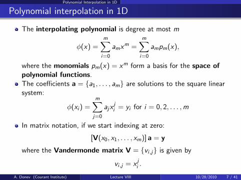
The interpolating polynomial is degree at most m

φ(x) =m∑i=0

amxm =m∑i=0

ampm(x),

where the monomials pm(x) = xm form a basis for the space ofpolynomial functions.The coefficients a = a1, . . . , am are solutions to the square linearsystem:

φ(xi ) =m∑j=0

ajxji = yi for i = 0, 2, . . . ,m

In matrix notation, if we start indexing at zero:

[V(x0, x1, . . . , xm)] a = y

where the Vandermonde matrix V = vi ,j is given by

vi ,j = x ji .



The Vandermonde approach

Va = x

One can prove by induction that

det V =∏j<k

(xk − xj)

which means that the Vandermonde system is non-singular and thus:The intepolating polynomial is unique if the nodes are distinct.

Polynomail interpolation is thus equivalent to solving a linear system.

However, it is easily seen that the Vandermonde matrix can be veryill-conditioned.

Solving a full linear system is also not very efficient because of thespecial form of the matrix.



Choosing the right basis functions

There are many mathematically equivalent ways to rewrite the uniqueinterpolating polynomial:

x2 − 2x + 4 = (x − 2)2.

One can think of this as choosing a different polynomial basisφ0(x), φ1(x), . . . , φm(x) for the function space of polynomials ofdegree at most m:

φ(x) =m∑i=0

aiφi (x)

For a given basis, the coefficients a can easily be found by solving thelinear system

φ(xj) =m∑i=0

aiφi (xj) = yj ⇒ Φa = y



Lagrange basis

Φa = y

This linear system will be trivial to solve if Φ = I, i.e., if

φi (xj) = δij =

1 if i = j

0 if i 6= j.

The φi (x) is itself a polynomial interpolant on the same nodes butwith function values δij , and is thus unique.

Note that the nodal polynomial

wm+1(x) =m∏i=0

(x − xi )

vanishes at all of the nodes but has degree m + 1.



Lagrange basis on 10 nodes

0 0.1 0.2 0.3 0.4 0.5 0.6 0.7 0.8 0.9 1−7

−6

−5

−4

−3

−2

−1

0

1

2A few Lagrange basis functions for 10 nodes

φ5

φ1

φ3



Lagrange interpolant

φi (xj) = δij

It can easily be seen that the following characteristic polynomialprovides the desired basis:

φi (x) =

∏j 6=i (x − xj)∏j 6=i (xi − xj)

=wm+1(x)

(x − xi )w ′m+1(xi )

The resulting Lagrange interpolation formula is

φ(x) =m∑i=0

yiφi (x) =m∑i=0

[yi∏

j 6=i (xi − xj)

]∏j 6=i

(x − xj)

This is useful analytically but expensive and cumbersome to usecomputationally!



Newton’s interpolation formula

By choosing a different basis we get different representations, andNewton’s choice is:

φi (x) = wi (x) =i−1∏j=0

(x − xj)

There is a simple recursive formula to calculate the coefficients a inthis basis, using Newton’s divided differences

D0i f = f (xi ) = yi

Dki =

Dk−1i+1 − Dk−1

i

xi+1 − xi.

Note that the first divided difference is

D1i =

f (xi+1)− f (xi )

xi+1 − xi≈ f ′ (xi ) ,

and D2i corresponds to second-order derivatives, etc.



Convergence, stability, etc.

We have lost track of our goal: How good is polynomial interpolation?

Assume we have a function f (x) that we are trying to approximateover an interval I = [x0, xm] using a polynomial interpolant.

Using Taylor series type analysis it is not hard to show that

∃ξ ∈ I such that Em(x) = f (x)− φ(x) =f (m+1) (ξ)

(m + 1)!

[m∏i=0

(x − xi )

].

Question: Does ‖Em(x)‖∞ = maxx∈I |f (x)| → 0 as m→∞.

For equi-spaced nodes, xi+1 = xi + h, a bound is

‖Em(x)‖∞ ≤hn+1

4(m + 1)

∥∥∥f (m+1) (x)∥∥∥∞.

The problem is that higher-order derivatives of seemingly nicefunctions can be unbounded!



Runge’s counter-example: f (x) = (1 + x2)−1

−5 −4 −3 −2 −1 0 1 2 3 4 5−5

−4

−3

−2

−1

0

1Runges phenomenon for 10 nodes

x

y



Uniformly-spaced nodes

Not all functions can be approximated well by an interpolatingpolynomial with equally-spaced nodes over an interval.

Interpolating polynomials of higher degree tend to be very oscillatoryand peaked, especially near the endpoints of the interval.

Even worse, the interpolation is unstable, under small perturbationsof the points y = y + δy,

‖δφ(x)‖∞ ≤2m+1

m log m‖δy‖∞

It is possible to improve the situation by using specially-chosennodes (e.g., Chebyshev nodes, discussed later), or by interpolatingderivatives (Hermite interpolation).

In general however, we conclude that interpolating usinghigh-degree polynomials is a bad idea!


Piecewise Polynomial Interpolation

Interpolation in 1D (Cleve Moler)



Piecewise Lagrange interpolants

The idea is to use a different low-degree polynomial function φi (x)in each interval Ii = [xi , xi+1].

Piecewise-constant interpolation: φ(0)i (x) = yi .

Piecewise-linear interpolation:

φ(1)i (x) = yi +

yi+1 − yixi+1 − xi

(x − xi ) for x ∈ Ii

For node spacing h the error estimate is now bounded and stable:∥∥∥f (x)− φ(1)(x)∥∥∥∞≤ h2

8

∥∥∥f (2) (x)∥∥∥∞



Piecewise Hermite interpolants

If we are given not just the function values but also the firstderivatives at the nodes:

zi = f ′(xi ),

we can find a cubic polynomial on every interval that interpolatesboth the function and the derivatives at the endpoints:

φi (xi ) = yi and φ′i (xi ) = zi

φi (xi+1) = yi+1 and φ′i (xi+1) = zi+1.

This is called the piecewise cubic Hermite interpolant.

If the derivatives are not available we can try to estimate zi ≈ φ′i (xi )(see MATLAB’s pchip).



Splines

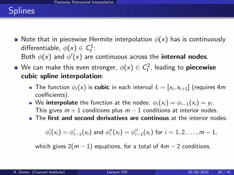
Note that in piecewise Hermite interpolation φ(x) has is continuouslydifferentiable, φ(x) ∈ C 1

I :Both φ(x) and φ′(x) are continuous across the internal nodes.

We can make this even stronger, φ(x) ∈ C 2I , leading to piecewise

cubic spline interpolation:

The function φi (x) is cubic in each interval Ii = [xi , xi+1] (requires 4mcoefficients).We interpolate the function at the nodes: φi (xi ) = φi−1(xi ) = yi .This gives m + 1 conditions plus m − 1 conditions at interior nodes.The first and second derivatives are continous at the interior nodes:

φ′i (xi ) = φ′i−1(xi ) and φ′′i (xi ) = φ′′i−1(xi ) for i = 1, 2, . . . ,m − 1,

which gives 2(m − 1) equations, for a total of 4m − 2 conditions.



Types of Splines

We need to specify two more conditions arbitrarily (for splines oforder k ≥ 3, there are k − 1 arbitrary conditions).

The most appropriate choice depends on the problem, e.g.:

Periodic splines, if y0 ≡ ym and we think of node 0 and node m as oneinterior node.Natural spline: φ′′(x0) = φ′′(x0) = 0.Not-a-knot condition: Enforce third-derivative continuity at x1 andxm−1.

Once the type of spline is chosen, finding the coefficients of the cubicpolynomials requires solving a tridiagonal linear system, which canbe done very fast (O(m)).



Nice properties of splines

Minimum curvature property:∫I

[φ′′(x)

]2dx ≤

∫I

[f ′′(x)

]2dx

The spline approximation converges for zeroth, first and secondderivatives (also third for uniformly-spaced nodes):

‖f (x)− φ(x)‖∞ ≤5

384· h4 ·

∥∥∥f (4) (x)∥∥∥∞∥∥f ′(x)− φ′(x)

∥∥∞ ≤

1

24· h3 ·

∥∥∥f (4) (x)∥∥∥∞∥∥f ′′(x)− φ′′(x)

∥∥∞ ≤

3

8· h2 ·

∥∥∥f (4) (x)∥∥∥∞



In MATLAB

c = polyfit(x , y , n) does least-squares polynomial of degree n which isinterpolating if n = length(x).

Note that MATLAB stores the coefficients in reverse order, i.e., c(1)is the coefficient of xn.

y = polyval(c, x) evaluates the interpolant at new points.

y1 = interp1(x , y , xnew ,′method ′) or if x is ordered use interp1q.

Method is one of ’linear’, ’spline’, ’cubic’.

The actual piecewise polynomial can be obtained and evaluated usingppval .



Interpolating (1 + x2)−1 in MATLAB

n=10;x=l i n s p a c e (−5 ,5 ,n ) ;y=(1+x . ˆ2 ) . ˆ ( −1 ) ;p l o t ( x , y , ’ ro ’ ) ; hold on ;

x f i n e=l i n s p a c e (−5 ,5 ,100) ;y f i n e=(1+ x f i n e . ˆ2 ) . ˆ ( −1 ) ;p l o t ( x f i n e , y f i n e , ’ b− ’ ) ;

c=p o l y f i t ( x , y , n ) ;y i n t e r p=p o l y v a l ( c , x f i n e ) ;p l o t ( x f i n e , y i n t e r p , ’ k−− ’ ) ;

y i n t e r p=i n t e r p 1 ( x , y , x f i n e , ’ s p l i n e ’ ) ;p l o t ( x f i n e , y i n t e r p , ’ k−− ’ ) ;% Or e q u i v a l e n t l y :pp=s p l i n e ( x , y ) ;y i n t e r p=ppva l ( pp , x f i n e )



Runge’s function with spline

−5 −4 −3 −2 −1 0 1 2 3 4 50

0.1

0.2

0.3

0.4

0.5

0.6

0.7

0.8

0.9

1Not−a−knot spline interpolant


Higher Dimensions

Regular grids

Now x = x1, . . . , xn ∈ Rn is a multidimensional data point. Focuson 2D since 3D is similar.

The easiest case is when the data points are all inside a rectangle

Ω = [x0, xmx ]× [y0, ymy ]

where m = mxmy and the nodes lie on a regular grid

xi ,j = xi , yj , fi ,j = f (xi ,j).

We can use separable basis functions:

φi ,j(x) = φi (x)φj(y).


Higher Dimensions

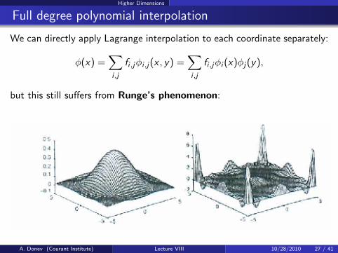
Full degree polynomial interpolation

We can directly apply Lagrange interpolation to each coordinate separately:

φ(x) =∑i ,j

fi ,jφi ,j(x , y) =∑i ,j

fi ,jφi (x)φj(y),

but this still suffers from Runge’s phenomenon:


Higher Dimensions

Piecewise-Polynomial Interpolation

Juse as in 1D, one can use a different interpolation functionφ(i ,j) : Ωi ,j → R in each rectange of the grid

Ωi ,j = [xi , xi+1]× [yj , yj+1].

For separable polynomials, the equivalent of piecewise linearinterpolation in 1D is the piecewise bilinear interpolation

φ(i ,j)(x , y) = φ(x)(i) (x) · φ(y)(j) (y),

where φ(x)(i) and φ

(y)(j) are linear function.

There are 4 unknown coefficients in φ(i ,j) that can be found from the4 data (function) values at the corners of rectangle Ωi ,j .

Note that the pieces of the interpolating function φ(i ,j)(x , y) are notlinear since they contain quadratic product terms xy : bilinearfunctions.This is because there is not a plane that passes through 4 genericpoints in 3D.


Higher Dimensions

Bilinear Interpolation

It is better to think in terms of a basis set φi ,j(x , y), where eachbasis functions is itself piecewise bilinear, and

φi ,j(xi ′ , yj ′) = δi ,i ′δj ,j ′ ⇒

φ(x) =∑i ,j

fi ,jφi ,j(x , y).

Furthermore, it is sufficient to look at a unit reference rectangleΩ = [0, 1]× [0, 1] since any other rectangle or even parallelogramcan be obtained from the reference one via a linear transformation:

Bi ,j Ω + bi ,j = Ωi ,j ,

and the same transformation can then be applied to the interpolationfunction:

φi ,j(x) = φ(Bi ,j x + bi ,j).


Higher Dimensions

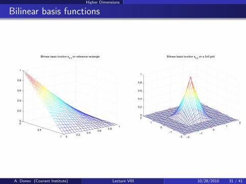
Bilinear Basis Functions

Consider one of the corners (0, 0) of the reference rectangle and thecorresponding basis φ0,0 restricted to Ω:

φ0,0(x , y) = (1− x)(1− y)

For an actual grid, the basis function corresponding to a given interiornode is simply a composite of 4 such bilinear terms, one for eachrectangle that has that interior node as a vertex: Often called a tentfunction.

If higher smoothness is required one can consider, for example,bicubic Hermite interpolation (when derivatives fx , fy and fxy areknown at the nodes as well).


Higher Dimensions

Bilinear basis functions

0

0.5

1 00.2

0.40.6

0.81

0

0.2

0.4

0.6

0.8

1

Bilinear basis function φ0,0

on reference rectangle

−2

−1

0

1

2

−2

−1

0

1

20

0.2

0.4

0.6

0.8

1

Bilinear basis function φ3,3

on a 5x5 grid


Higher Dimensions

Bicubic basis functions

0

0.2

0.4

0.6

0.8

1 0

0.2

0.4

0.6

0.8

10

0.2

0.4

0.6

0.8

1

−2

−1

0

1

2

−2

−1

0

1

2−0.2

0

0.2

0.4

0.6

0.8

1

1.2

Bicubic basis function φ3,3

on a 5x5 grid


Higher Dimensions

Irregular (Simplicial) Meshes

Any polygon can be triangulated into arbitrarily many disjoint triangles.Similarly tetrahedral meshes in 3D.


Higher Dimensions

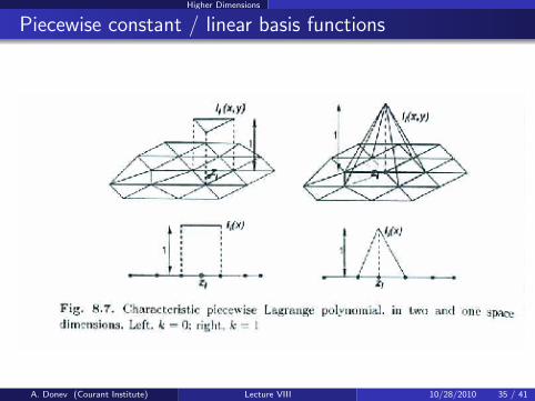
Basis functions on triangles

For irregular grids the x and y directions are no longer separable.

But the idea of using basis functions φi ,j , a reference triangle, andpiecewise polynomial interpolants still applies.

For a linear function we need 3 coefficients (x , y , const), for quadratic6 (x , y , x2, y2, xy , const):


Higher Dimensions

Piecewise constant / linear basis functions


Higher Dimensions

In MATLAB

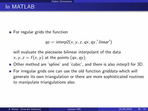
For regular grids the function

qz = interp2(x , y , z , qx , qy ,′ linear ′)

will evaluate the piecewise bilinear interpolant of the datax , y , z = f (x , y) at the points (qx , qy).

Other method are ’spline’ and ’cubic’, and there is also interp3 for 3D.

For irregular grids one can use the old function griddata which willgenerate its own triangulation or there are more sophisticated routinesto manipulate triangulations also.


Higher Dimensions

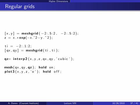
Regular grids

[ x , y ] = meshgrid ( −2 : . 5 : 2 , −2 : . 5 : 2 ) ;z = x .∗ exp(−x .ˆ2−y . ˆ 2 ) ;

t i = −2 : . 1 : 2 ;[ qx , qy ] = meshgrid ( t i , t i ) ;

qz= i n t e r p 2 ( x , y , z , qx , qy , ’ c ub i c ’ ) ;

mesh ( qx , qy , qz ) ; hold on ;p lot3 ( x , y , z , ’ o ’ ) ; hold o f f ;


Higher Dimensions

MATLAB’s interp2

−2

−1

0

1

2

−2

−1

0

1

2

−0.4

−0.3

−0.2

−0.1

0

0.1

0.2

0.3

0.4

−1 −0.8 −0.6 −0.4 −0.2 0 0.2 0.4 0.6 0.8 1−5

−4

−3

−2

−1

0

1

2Function and approximations for n=10

Actual

Equi−spaced nodes

Standard approx

Gauss nodes

Spectral approx


Higher Dimensions

Irregular grids

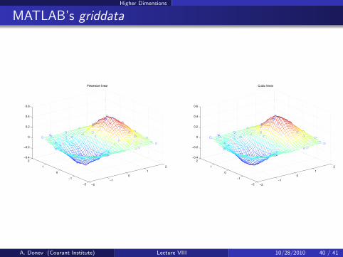
x = rand (100 ,1)∗4−2; y = rand (100 ,1)∗4−2;z = x .∗ exp(−x .ˆ2−y . ˆ 2 ) ;

t i = −2 : . 1 : 2 ;[ qx , qy ] = meshgrid ( t i , t i ) ;

qz= g r i d d a t a ( x , y , z , qx , qy , ’ c ub i c ’ ) ;

mesh ( qx , qy , qz ) ; hold on ;p lot3 ( x , y , z , ’ o ’ ) ; hold o f f ;


Higher Dimensions

MATLAB’s griddata

−2

−1

0

1

2

−2

−1

0

1

2

−0.4

−0.2

0

0.2

0.4

0.6

Piecewise linear

−2

−1

0

1

2

−2

−1

0

1

2

−0.4

−0.2

0

0.2

0.4

0.6

Cubic linear


Conclusions

Conclusions/Summary

Interpolation means approximating function values in the interior of adomain when there are known samples of the function at a set ofinterior and boundary nodes.

Given a basis set for the interpolating functions, interpolationamounts to solving a linear system for the coefficients of the basisfunctions.

Polynomial interpolants in 1D can be constructed using several basis.

Using polynomial interpolants of high order is a bad idea: Notaccurate and not stable!

Instead, it is better to use piecewise polynomial interpolation:constant, linear, Hermite cubic, cubic spline interpolant on eachinterval.In higher dimensions one must be more careful about how the domainis split into disjoint elements (analogues of intervals in 1D): regulargrids (separable basis such as bilinear), or simplicial meshes(triangular or tetrahedral).


numerical methods i polynomial interpolationdonev/teaching/nmi-fall2010/... · spline interpolation...

Documents