adaptive resource control - sztakicsaji/csaji-phd-thesis.pdf · a carpenter and a geometrician both...
TRANSCRIPT
ADAPTIVE RESOURCE CONTROL
Machine Learning Approaches to Resource Allocation
in Uncertain and Changing Environments
P h. D. T h e s i s
Balázs Csanád Csáji
Supervisor: László Monostori, D.Sc.
Faculty of Informatics (IK),
Eötvös Loránd University (ELTE)
Doctoral School of Computer Science,
Foundations and Methods in Informatics Ph.D. Program,
Chairman: Prof. János Demetrovics, Member of HAS
Computer and Automation Research Institute (SZTAKI),
Hungarian Academy of Sciences (HAS, MTA)
Budapest, Hungary, 2008
[...] καὶ τὴν ἀκρίβειαν μὴ ὁμοίως ἐν ἅπασιν ἐπιζητεῖν, ἀλλ᾿ ἐν ἑκάστοις κατὰ τὴν
ὑποκειμένην ὕλην καὶ ἐπὶ τοσοῦτον ἐφ᾿ ὅσον οἰκεῖον τῇ μεθόδῳ. καὶ γὰρ τέκτων καὶ
γεωμέτρης διαφερόντως ἐπιζητοῦσι τὴν ὀρθήν: ὃ μὲν γὰρ ἐφ᾿ ὅσον χρησίμη πρὸς τὸ ἔργον,
ὃ δὲ τί ἐστιν ἢ ποῖόν τι: θεατὴς γὰρ τἀληθοῦς. τὸν αὐτὸν δὴ τρόπον καὶ ἐν τοῖς ἄλλοις
ποιητέον, ὅπως μὴ τὰ πάρεργα τῶν ἔργων πλείω γίνηται. (Aristotle, Nicomachean Ethics,
1098a; based on: Ingram Bywater, editor, Oxford, Clarendon Press, 1894)
[...] we must not look for equal exactness in all departments of study, but only such
as belongs to the subject matter of each, and in such a degree as is appropriate to the
particular line of enquiry. A carpenter and a geometrician both try to find a right angle,
but in different ways; the former is content with that approximation to it which satisfies
the purpose of his work; the latter, being a student of truth, seeks to find its essence or
essential attributes. We should therefore proceed in the same manner in other subjects
also, and not allow side issues to outbalance the main task in hand. (Aristotle in 23
Volumes, Vol. 19, translated by Harris Rackham, Harvard University Press, 1934)

Declaration
Herewith I confirm that all of the research described in this dissertation is my own originalwork and expressed in my own words. Any use made within it of works of other authors inany form, e.g., ideas, figures, text, tables, are properly indicated through the application ofcitations and references. I also declare that no part of the dissertation has been submittedfor any other degree — either from the Eötvös Loránd University or another institution.
Balázs Csanád Csáji
Budapest, April 2008
1

Acknowledgments
Though, the thesis is my own work, I received many support from my colleagues and family.Without them, the dissertation would not be the same. I would like to take the opportunityto express my gratitude here to all who helped and encouraged me during my studies.
First of all, I want to thank those people that had a direct influence on my thesis. Theseinclude first and foremost my supportive supervisor, László Monostori, but also the peoplewhom I have collaborated with at the Engineering and Management Intelligence (EMI)Laboratory of the Computer and Automation Research Institute (SZTAKI).
Furthermore, I warmly thank Csaba Szepesvári for the many helpful discussions onMarkov decision processes. I am very grateful to László Gerencsér, as well, from whom Ilearned a lot about stochastic models. I am also thankful for expanding my knowledge onmachine learning to László Györfi. Finally, the first researcher who motivated my interestin artificial intelligence research during my graduate studies was András Lőrincz.
I am also grateful for the Ph.D. scholarship that I received from the Faculty of Informatics(IK) of the Eötvös Loránd University (ELTE) and, later, for the young researcher scholarshipof the Hungarian Academy of Sciences (HAS, MTA). I greatly acknowledge the contributionof SZTAKI, as well, where I performed the research presented in the dissertation.
Last but not least, I am very thankful for the support and encouragement of my parentsand family, especially, for the continuous help and care of my wife, Hildegard Anna Stift.
2

Abstract
The dissertation aims at studying resource allocation problems (RAPs) in uncertain andchanging environments. In order to do this, first a brief introduction to the motivations andclassical RAPs is given in Chapter 1, followed by a section on Markov decision processes(MDPs) which constitute the basis of the approach. The core of the thesis consists of twoparts, the first deals with uncertainties, namely, with stochastic RAPs, while the secondstudies the effects of changes in the environmental dynamics on learning algorithms.
Chapter 2, the first core part, investigates stochastic RAPs with scarce, reusable re-sources and non-preemtive, interconnected tasks having temporal extensions. These RAPsare natural generalizations of several standard resource management problems, such asscheduling and transportation ones. First, reactive solutions are considered and definedas policies of suitably reformulated MDPs. It is highlighted that this reformulation hasseveral favorable properties, such as it has finite state and action spaces, it is acyclic, henceall policies are proper and the space of policies can be safely restricted. Proactive solutionsare also proposed and defined as policies of special partially observable MDPs. Next, rein-forcement learning (RL) methods, such as fitted Q-learning, are suggested for computing apolicy. In order to compactly maintain the value function, two representations are studied:hash tables and support vector regression (SVR), particularly, ν-SVRs. Several additionalimprovements, such as the application of rollout algorithms in the initial phases, actionspace decomposition, task clustering and distributed sampling are investigated, as well.
Chapter 3, the second core part, studies the possibility of applying value function basedRL methods in cases when the environment may change over time. First, theorems arepresented which show that the optimal value function and the value function of a fixed controlpolicy Lipschitz continuously depend on the immediate-cost function and the transition-probability function, assuming a discounted MDP. Dependence on the discount factor isalso analyzed and shown to be non-Lipschitz. Afterwards, the concept of (ε, δ)-MDPs isintroduced, which is a generalization of MDPs and ε-MDPs. In this model the transition-probability function and the immediate-cost function may vary over time, but the changesmust be asymptotically bounded. Then, learning in changing environments is investigated.A general relaxed convergence theorem for stochastic iterative algorithms is presented andillustrated through three classical examples: value iteration, Q-learning and TD-learning.
Finally, in Chapter 4, results of numerical experiments on both benchmark and industry-related problems are shown. The effectiveness of the proposed adaptive resource allocationapproach as well as learning in presence of disturbances and changes are demonstrated.
3

Contents
Declaration 1
Acknowledgments 2
Abstract 3
Contents 4
1 Introduction 7
1.1 Resource Allocation . . . . . . . . . . . . . . . . . . . . . . . . . . . . . . . . 81.1.1 Industrial Motivations . . . . . . . . . . . . . . . . . . . . . . . . . . . 81.1.2 Curse(s) of Dimensionality . . . . . . . . . . . . . . . . . . . . . . . . . 81.1.3 Related Literature . . . . . . . . . . . . . . . . . . . . . . . . . . . . . 91.1.4 Classical Problems . . . . . . . . . . . . . . . . . . . . . . . . . . . . . 10
» Job-Shop Scheduling . . . . . . . . . . . . . . . . . . . . . . . . . . 10» Traveling Salesman . . . . . . . . . . . . . . . . . . . . . . . . . . . 11» Container Loading . . . . . . . . . . . . . . . . . . . . . . . . . . . 11
1.2 Markov Decision Processes . . . . . . . . . . . . . . . . . . . . . . . . . . . . . 131.2.1 Control Policies . . . . . . . . . . . . . . . . . . . . . . . . . . . . . . . 141.2.2 Value Functions . . . . . . . . . . . . . . . . . . . . . . . . . . . . . . . 141.2.3 Bellman Equations . . . . . . . . . . . . . . . . . . . . . . . . . . . . . 151.2.4 Approximate Solutions . . . . . . . . . . . . . . . . . . . . . . . . . . . 161.2.5 Partial Observability . . . . . . . . . . . . . . . . . . . . . . . . . . . . 16
1.3 Main Contributions . . . . . . . . . . . . . . . . . . . . . . . . . . . . . . . . . 181.3.1 Stochastic Resource Allocation . . . . . . . . . . . . . . . . . . . . . . 181.3.2 Varying Environments . . . . . . . . . . . . . . . . . . . . . . . . . . . 19
2 Stochastic Resource Allocation 21
2.1 Markovian Resource Control . . . . . . . . . . . . . . . . . . . . . . . . . . . . 212.1.1 Deterministic Framework . . . . . . . . . . . . . . . . . . . . . . . . . 22
» Feasible Resource Allocation . . . . . . . . . . . . . . . . . . . . . . 22» Performance Measures . . . . . . . . . . . . . . . . . . . . . . . . . 23» Demonstrative Examples . . . . . . . . . . . . . . . . . . . . . . . . 24
4
CONTENTS 5
» Computational Complexity . . . . . . . . . . . . . . . . . . . . . . . 242.1.2 Stochastic Framework . . . . . . . . . . . . . . . . . . . . . . . . . . . 24
» Stochastic Dominance . . . . . . . . . . . . . . . . . . . . . . . . . 25» Solution Classification . . . . . . . . . . . . . . . . . . . . . . . . . 25
2.1.3 Reactive Resource Control . . . . . . . . . . . . . . . . . . . . . . . . . 26» Problem Reformulation . . . . . . . . . . . . . . . . . . . . . . . . . 27» Favorable Features . . . . . . . . . . . . . . . . . . . . . . . . . . . 28» Composable Measures . . . . . . . . . . . . . . . . . . . . . . . . . 29» Reactive Solutions . . . . . . . . . . . . . . . . . . . . . . . . . . . 29
2.1.4 Proactive Resource Control . . . . . . . . . . . . . . . . . . . . . . . . 30» Proactive Solutions . . . . . . . . . . . . . . . . . . . . . . . . . . . 31
2.2 Machine Learning Approaches . . . . . . . . . . . . . . . . . . . . . . . . . . . 312.2.1 Reinforcement Learning . . . . . . . . . . . . . . . . . . . . . . . . . . 31
» Fitted Value Iteration . . . . . . . . . . . . . . . . . . . . . . . . . 32» Fitted Policy Iteration . . . . . . . . . . . . . . . . . . . . . . . . . 32» Fitted Q-learning . . . . . . . . . . . . . . . . . . . . . . . . . . . . 33» Evaluation by Simulation . . . . . . . . . . . . . . . . . . . . . . . . 34» The Boltzmann Formula . . . . . . . . . . . . . . . . . . . . . . . . 34
2.2.2 Cost-to-Go Representations . . . . . . . . . . . . . . . . . . . . . . . . 34» Feature Vectors . . . . . . . . . . . . . . . . . . . . . . . . . . . . . 35» Hash Tables . . . . . . . . . . . . . . . . . . . . . . . . . . . . . . . 35» Support Vector Regression . . . . . . . . . . . . . . . . . . . . . . . 36
2.2.3 Additional Improvements . . . . . . . . . . . . . . . . . . . . . . . . . 40» Rollout Algorithms . . . . . . . . . . . . . . . . . . . . . . . . . . . 40» Action Space Decomposition . . . . . . . . . . . . . . . . . . . . . . 41» Clustering the Tasks . . . . . . . . . . . . . . . . . . . . . . . . . . 42
2.2.4 Distributed Systems . . . . . . . . . . . . . . . . . . . . . . . . . . . . 43» Agent Based Approaches . . . . . . . . . . . . . . . . . . . . . . . . 43» Parallel Optimization . . . . . . . . . . . . . . . . . . . . . . . . . . 45» Distributed Sampling . . . . . . . . . . . . . . . . . . . . . . . . . . 46
3 Varying Environments 48
3.1 Changes in the Dynamics . . . . . . . . . . . . . . . . . . . . . . . . . . . . . 493.1.1 Transition Changes . . . . . . . . . . . . . . . . . . . . . . . . . . . . . 493.1.2 Cost Changes . . . . . . . . . . . . . . . . . . . . . . . . . . . . . . . . 503.1.3 Discount Changes . . . . . . . . . . . . . . . . . . . . . . . . . . . . . 513.1.4 Action-Value Changes . . . . . . . . . . . . . . . . . . . . . . . . . . . 513.1.5 Optimal Cost-to-Go Changes . . . . . . . . . . . . . . . . . . . . . . . 523.1.6 Further Remarks . . . . . . . . . . . . . . . . . . . . . . . . . . . . . . 53
» Average Cost Case . . . . . . . . . . . . . . . . . . . . . . . . . . . 54» Simulation Lemma . . . . . . . . . . . . . . . . . . . . . . . . . . . 54» State and Action Changes . . . . . . . . . . . . . . . . . . . . . . . 54

CONTENTS 6
» Counterexamples . . . . . . . . . . . . . . . . . . . . . . . . . . . . 553.2 Learning in Varying Environments . . . . . . . . . . . . . . . . . . . . . . . . 56
3.2.1 Unified Learning Framework . . . . . . . . . . . . . . . . . . . . . . . . 56» Generalized Value Functions . . . . . . . . . . . . . . . . . . . . . . 56» Kappa Approximation . . . . . . . . . . . . . . . . . . . . . . . . . 56» Generalized Value Iteration . . . . . . . . . . . . . . . . . . . . . . 57» Asymptotic Convergence Bounds . . . . . . . . . . . . . . . . . . . 57
3.2.2 Varying Markov Decision Processes . . . . . . . . . . . . . . . . . . . . 583.2.3 Stochastic Iterative Algorithms . . . . . . . . . . . . . . . . . . . . . . 60
» Time-Dependent Update . . . . . . . . . . . . . . . . . . . . . . . . 60» Main Assumptions . . . . . . . . . . . . . . . . . . . . . . . . . . . 60» Approximate Convergence . . . . . . . . . . . . . . . . . . . . . . . 61» An Alternating Example . . . . . . . . . . . . . . . . . . . . . . . . 62» A Pathological Example . . . . . . . . . . . . . . . . . . . . . . . . 62
3.2.4 Learning in Varying MDPs . . . . . . . . . . . . . . . . . . . . . . . . 64» Asynchronous Value Iteration . . . . . . . . . . . . . . . . . . . . . 64» Q-learning . . . . . . . . . . . . . . . . . . . . . . . . . . . . . . . . 65» Temporal Difference Learning . . . . . . . . . . . . . . . . . . . . . 65
4 Experimental Results 67
4.1 Stochastic Resource Allocation . . . . . . . . . . . . . . . . . . . . . . . . . . 674.1.1 Testing Methodology . . . . . . . . . . . . . . . . . . . . . . . . . . . . 674.1.2 Benchmark Datasets . . . . . . . . . . . . . . . . . . . . . . . . . . . . 684.1.3 Distributed Sampling . . . . . . . . . . . . . . . . . . . . . . . . . . . . 704.1.4 Industry Related Tests . . . . . . . . . . . . . . . . . . . . . . . . . . . 704.1.5 Clustering Experiments . . . . . . . . . . . . . . . . . . . . . . . . . . 72
4.2 Varying Environments . . . . . . . . . . . . . . . . . . . . . . . . . . . . . . . 734.2.1 Adaptation to Disturbances . . . . . . . . . . . . . . . . . . . . . . . . 734.2.2 Varying Grid Worlds . . . . . . . . . . . . . . . . . . . . . . . . . . . . 74
5 Conclusion 77
5.1 Managing Uncertainties . . . . . . . . . . . . . . . . . . . . . . . . . . . . . . 775.2 Dealing with Changes . . . . . . . . . . . . . . . . . . . . . . . . . . . . . . . 785.3 Further Research Directions . . . . . . . . . . . . . . . . . . . . . . . . . . . . 79
Appendix: Proofs 81
Abbreviations 94
Notations 96
Bibliography 99
Chapter 1
Introduction
Information technology has been making an explosion-like progress since the middle of thepast century. However, as computer science broke out from laboratories and classroomsand started to deal with “real world” problems, it had to face major difficulties. Namely,in practise, we mostly have only incomplete and uncertain information on the system andthe environment that we must work with, additionally, they may even change dynamically,the problem may be non-stationary. Moreover, we also have to face complexity issues, viz.,even if we deal with static, highly simplified and abstract problems and it can be knownthat the solution exists and can be attained in finitely many steps, the problem could stillbe intractable, viz., we might not have enough computation power (or even enough storagespace) to achieve it in practise, as this is the case, e.g., with many NP-hard problems.
One way to overcome these difficulties is to apply machine learning techniques. It meansdesigning systems which can adapt their behavior to the current state of the environment,extrapolate their knowledge to the unknown cases and learn how to optimize the system.These approaches often use statistical methods and satisfy with approximate, suboptimal
but tractable solutions concerning both computational demands and storage space.The importance of learning was recognized even by the founders of computer science. It
is well known, e.g., that John von Neumann (1948) was keen on artificial life and, besidesmany other things, designed self-organizing automata. Alan Turing (1950) can be anotherexample, who in his famous paper, which can be treated as one of the starting articles ofartificial intelligence research, wrote that instead of designing extremely complex and largesystems, we should design programs that can learn how to work efficiently by themselves.
In the dissertation we consider an important problem with many practical applications,which has all the difficulties mentioned in the previous parts, namely: resource allocation.In this chapter, first, a brief introduction to resource allocation is given followed by a sec-tion on Markov decision processes (MDPs), since they constitute the basis of the presentedapproach. At the end of Chapter 1 the main contributions of the dissertation are summa-rized. Chapter 2 deals with uncertainties concerning resource allocation, namely, it defines ageneralized framework for stochastic problems, then, an MDP based reformulation is givenand efficient solution methods are suggested applying various machine learning techniques,such as reinforcement learning, support vector regression and clustering. Chapter 3 studies
7
1.1. Resource Allocation 8
the effects of environmental changes on learning algorithms. First, different value functionbounds for environmental changes are presented followed by an analysis of stochastic iter-ative algorithms in a special class of non-stationary environments. Finally, in Chapter 4results of numerical experiments on benchmark and industry-related data are presented.
1.1 Resource Allocation
Resource allocation problems (RAPs) are of high practical importance, since they arise inmany diverse fields, such as manufacturing production control (e.g., production scheduling),warehousing (e.g., storage allocation), fleet management (e.g., freight transportation), per-sonnel management (e.g., in an office), scheduling of computer programs (e.g., in massivelyparallel GRID systems), managing a construction project or controlling a cellular mobilenetwork. RAPs are also central to management science (Powell and Van Roy, 2004). Inthe thesis we consider optimization problems that include the assignment of a finite set ofreusable resources to non-preemtive, interconnected tasks that have stochastic durations andeffects. Our main objective in the thesis is to investigate efficient decision-making processeswhich can deal with the allocation of scarce resources over time with a goal of optimizingthe objectives. For “real world” applications, it is important that the solution should be ableto deal with large-scale problems and handle environmental changes, as well.
1.1.1 Industrial Motivations
One of our main motivations for investigating RAPs is to enhance manufacturing productioncontrol. Regarding contemporary manufacturing systems, difficulties arise from unexpectedtasks and events, non-linearities, and a multitude of interactions while attempting to controlvarious activities in dynamic shop floors. Complexity and uncertainty seriously limit theeffectiveness of conventional production control approaches (e.g., deterministic scheduling).In the thesis we apply mathematical programming and machine learning (ML) techniques toachieve the suboptimal control of a generalized class of stochastic RAPs, which can be vital toan intelligent manufacturing system (IMS). The term of IMS can be attributed to a tentativeforecast of Hatvany and Nemes (1978). In the early 80s IMSs were outlined as the nextgeneration of manufacturing systems that utilize the results of artificial intelligence researchand were expected to solve, within certain limits, unprecedented, unforeseen problems onthe basis of even incomplete and imprecise information. Naturally, the applicability of thedifferent proposed solutions to RAPs are not limited to industrial problems.
1.1.2 Curse(s) of Dimensionality
Different kinds of RAPs have a huge number of exact and approximate solution meth-ods, e.g., (see Pinedo, 2002) in the case of scheduling problems. However, these methodsprimarily deal with the static (and often strictly deterministic) variants of the various prob-lems and, mostly, they are not aware of uncertainties and changes. Special (deterministic)RAPs which appear in the field of combinatorial optimization, e.g., the traveling salesmanproblem (TSP) or the job-shop scheduling problem (JSP), are strongly NP-hard and, more-
1.1. Resource Allocation 9
over, they do not have any good polynomial-time approximation, either (Lawler et al., 1993;Lovász and Gács, 1999). In the stochastic case, RAPs can be often formulated as Markov
decision processes (MDPs) and by applying dynamic programming (DP) methods, in theory,they can be solved optimally. However, due to the phenomenon that was named curse of
dimensionality by Bellman, these methods are highly intractable in practice. The “curse”refers to the combinatorial explosion of the required computation as the size of the problemincreases. Some authors, e.g., Powell and Van Roy (2004), talk about even three types ofcurses concerning DP algorithms. This has motivated approximate approaches that requirea more tractable computation, but often yield suboptimal solutions (Bertsekas, 2005).
1.1.3 Related Literature
It is beyond our scope to give a general overview on different solutions to RAPs, hence, weonly concentrate on the part of the literature that is closely related to our approach. Oursolution belongs to the class of approximate dynamic programming (ADP) algorithms whichconstitute a broad class of discrete-time control techniques. Note that ADP methods thattake an actor-critic point of view are often called reinforcement learning (RL).
Zhang and Dietterich (1995) were the first to apply an RL technique for a special RAP.They used the TD(λ) method with iterative repair to solve a static scheduling problem,namely, the NASA space shuttle payload processing problem. Since then, a number of pa-pers have been published that suggested using RL for different RAPs. The first reactive(closed-loop) solution to scheduling problems using ADP algorithms was briefly describedin (Schneider et al., 1998). Riedmiller and Riedmiller (1999) used a multilayer perceptron
(MLP) based neural RL approach to learn local heuristics. Aydin and Öztemel (2000) ap-plied a modified version of Q-learning to learn dispatching rules for production scheduling.In (Csáji et al., 2003, 2004; Csáji and Monostori, 2005b,a, 2006a,b; Csáji et al., 2006) multi-agent based versions of ADP techniques were used for solving dynamic scheduling problems.
Powell and Van Roy (2004) presented a formal framework for RAPs and they appliedADP to give a general solution to their problem. Later, a parallelized solution to the pre-viously defined problem was given by Topaloglu and Powell (2005). Note that our RAPframework, presented in Chapter 2, differs from the one in (Powell and Van Roy, 2004),since in our system the goal is to accomplish a set of tasks that can have widely differ-ent stochastic durations and precedence constraints between them, while the approach ofPowell and Van Roy (2004) concerns with satisfying many similar demands arriving stochas-tically over time with demands having unit durations but not precedence constraints.
Recently, support vector machines (SVMs) were applied by Gersmann and Hammer(2005) to improve iterative repair (local search) strategies for resource constrained project
scheduling problems (RCPSPs). An agent-based resource allocation system with MDP-induced preferences was presented in stepDolgov2006. Beck and Wilson (2007) gave proac-tive solutions for job-shop scheduling problems based on the combination of Monte Carlo
simulation, solutions of the associated deterministic problem, and either constraint program-ming or tabu-search. Finally, the effects of environmental changes on the convergence ofreinforcement learning algorithms was theoretically analyzed by Szita et al. (2002).

1.1. Resource Allocation 10
1.1.4 Classical Problems
In this section we give a brief introduction to RAPs through three classical problems: job-shop scheduling, traveling salesman and container loading. All of these problems are knownto be NP-hard. Throughout the thesis we will apply them to demonstrate our ideas.
Job-Shop Scheduling
First, we consider the classical job-shop scheduling problem (JSP) which is a standard de-terministic RAP (Pinedo, 2002). We have a set of jobs, J = J1, . . . , Jn, to be processedthrough a set of machines, M = M1, . . . ,Mk. Each j ∈ J consists of a sequence of nj
tasks, for each task tji ∈ T , where i ∈ 1, . . . , nj, there is a machine mji ∈ M which canprocess the task, and a processing time pji ∈ N. The aim of the optimization is to find afeasible schedule which minimizes a given performance measure. A solution, i.e., a schedule,is a suitable “task to starting time” assignment, Figure 1.1 presents an example schedule.The concept of “feasibility” will be defined in Chapter 2. In the case of JSP a feasibleschedule can be associated with an ordering of the tasks, i.e., the order in which they willbe executed on the machines. There are many types of performance measures available forJSP, but probably the most commonly applied one is the maximum completion time of thetasks, also called “makespan”. In case of applying makespan, JSP can be interpreted as theproblem of finding a schedule which completes all tasks in every job as soon as possible.
Figure 1.1: A possible solution to JSP, presented in a Gantt chart. Tasks having the samecolor belong to the same job and should be processed in the given order. Thevertical gray dotted line indicates the maximum completion time of the tasks.
Later, we will study an extension of JSP, the flexible job-shop scheduling problem (FJSP).In FJSP the machines may be interchangeable, i.e., there may be tasks that can be executedon several machines. In this case the processing times are given by a partial function,p : M× T → N. Recall that a partial function, denoted by “ →”, is a binary relation thatassociates the elements of its domain set with at most one element of its range set.
An even more general version of JSP, which is often referred to as resource constrained
project scheduling problem (RCPSP), arises when the tasks may require several resources,such as machines and workers, simultaneously, in order to be executed (Pinedo, 2002).

1.1. Resource Allocation 11
Traveling Salesman
One of the basic transportation problems is the famous traveling salesman problem (TSP)that can be stated as follows. Given a number of cities and the costs of travelings betweenthem, which is the least-cost round-trip route that visits each city exactly once and thenreturns to the starting city (Papadimitriou, 1994). Several variants of TSP are known, herewe present one of the standard versions. It can be formally characterized by a connected,undirected, edge-weighted graph G = 〈V,E,w〉, where the components are as follows. Thevertex set, V = 1, . . . , n, is corresponding to the set of “cities”, E ⊆ V × V is the set ofedges which represents the “roads” between the cities, and function w : E → N defines theweights of the edges: the durations of the trips. The aim of the optimization is to find aHamilton-circuit with the smallest possible weight. Note that a Hamilton-circuit is a graphcycle that starts at a vertex, passes through every vertex exactly once and, finally, returnsto the starting vertex. Take a look at Figure 1.2 for an example Hamilton-circuit.
Figure 1.2: A possible solution to TSP, a path in the graph. The black edges constitute aHamilton-circuit in the given connected, undirected, edge-weighted graph.
Container Loading
Our final classical example is the container loading problem (CLP) which is an inventorymanagement problem (Davies and Bischoff, 1999). CLP is related to the bin packing prob-lem with the objective of high volumetric utilization. It involves the placement of a set ofitems in a container. In practical applications there are a number of requirements concern-ing container loading, such as stacking conditions, cargo stability, visibility and accessibilityconsiderations. Now, as a simplification, we concentrate only on the weight distribution ofthe loaded container, focusing on the location of the center of gravity (CoG). The exactrequirements concerning CoG depend on the specific application, especially on the means oftransport. In aircraft loading or loading containers lifted by cranes, for example, the CoGhas to be located in the center of the container. In contrast, in road transport, it is oftenpreferred to have the CoG above the axles of the vehicle (Kovács and Beck, 2007).
1.1. Resource Allocation 12
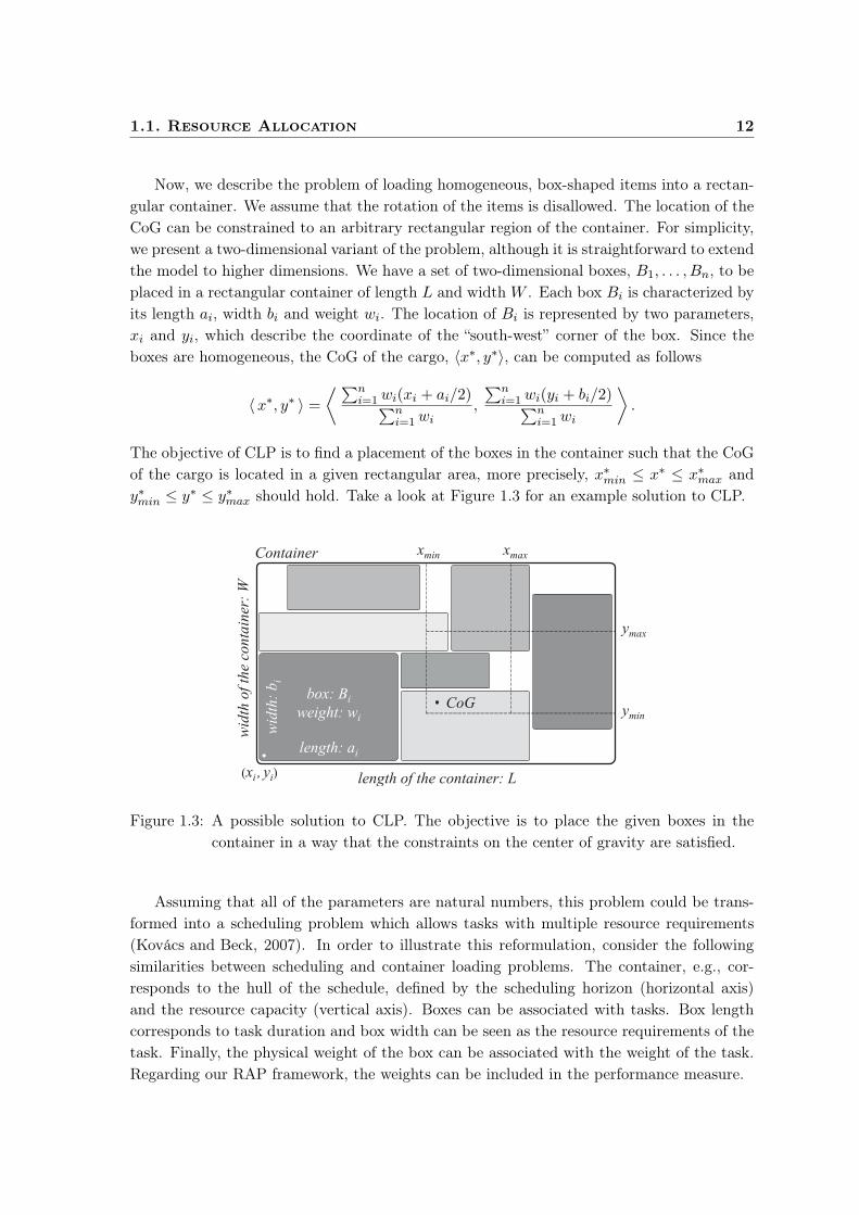
Now, we describe the problem of loading homogeneous, box-shaped items into a rectan-gular container. We assume that the rotation of the items is disallowed. The location of theCoG can be constrained to an arbitrary rectangular region of the container. For simplicity,we present a two-dimensional variant of the problem, although it is straightforward to extendthe model to higher dimensions. We have a set of two-dimensional boxes, B1, . . . , Bn, to beplaced in a rectangular container of length L and width W . Each box Bi is characterized byits length ai, width bi and weight wi. The location of Bi is represented by two parameters,xi and yi, which describe the coordinate of the “south-west” corner of the box. Since theboxes are homogeneous, the CoG of the cargo, 〈x∗, y∗〉, can be computed as follows
〈x∗, y∗ 〉 =
⟨ ∑ni=1wi(xi + ai/2)∑n
i=1wi,
∑ni=1wi(yi + bi/2)∑n
i=1wi
⟩.
The objective of CLP is to find a placement of the boxes in the container such that the CoGof the cargo is located in a given rectangular area, more precisely, x∗min ≤ x∗ ≤ x∗max andy∗min ≤ y∗ ≤ y∗max should hold. Take a look at Figure 1.3 for an example solution to CLP.
Figure 1.3: A possible solution to CLP. The objective is to place the given boxes in thecontainer in a way that the constraints on the center of gravity are satisfied.
Assuming that all of the parameters are natural numbers, this problem could be trans-formed into a scheduling problem which allows tasks with multiple resource requirements(Kovács and Beck, 2007). In order to illustrate this reformulation, consider the followingsimilarities between scheduling and container loading problems. The container, e.g., cor-responds to the hull of the schedule, defined by the scheduling horizon (horizontal axis)and the resource capacity (vertical axis). Boxes can be associated with tasks. Box lengthcorresponds to task duration and box width can be seen as the resource requirements of thetask. Finally, the physical weight of the box can be associated with the weight of the task.Regarding our RAP framework, the weights can be included in the performance measure.

1.2. Markov Decision Processes 13
1.2 Markov Decision Processes
Stochastic control problems are often modeled by MDPs that constitute a fundamentaltool for computational learning theory. The theory of MDPs has grown extensively sinceBellman introduced the discrete stochastic variant of the optimal control problem in 1957.These kinds of stochastic optimization problems have great importance in diverse fields,such as engineering, manufacturing, medicine, finance or social sciences. Several solutionmethods are known, e.g., from the field of [neuro-]dynamic programming (NDP) or reinforce-ment learning (RL), which compute or approximate the optimal control policy of an MDP.These methods succeeded in solving many different problems, such as transportation andinventory control (Van Roy et al., 1996), channel allocation (Singh and Bertsekas, 1997),robotic control (Kalmár et al., 1998), logical games and problems from financial mathemat-ics. Many applications of RL and NDP methods are also considered by the textbooks ofBertsekas and Tsitsiklis (1996), Sutton and Barto (1998) and Feinberg and Shwartz (2002).
This section contains the basic definitions, the applied notations and some preliminaries.MDPs are of special interest for us, since they constitute the fundamental theory of ourapproach. In Chapter 2, e.g., generalized stochastic RAPs are presented and, in order toapply machine learning techniques to solve them, they are reformulated as MDPs. Later, inChapter 3, environmental changes are investigated within the concept of MDPs, as well.
Definition 1 By a (finite, discrete-time, stationary, fully observable) Markov decision pro-
cess (MDP) we mean a stochastic system characterized by a 6-tuple 〈X,A,A, p, g, α〉, where
the components are as follows: X is a finite set of discrete states and A is a finite set of con-
trol actions. Mapping A : X → P(A) is the availability function that renders each state a set
of actions available in that state where P denotes the power set. The transition-probability
function is given by p : X × A → ∆(X), where ∆(X) is the space of probability distribu-
tions over X. Let p(y |x, a) denote the probability of arrival at state y after executing action
a ∈ A(x) in state x. The immediate-cost function is defined by g : X×A → R, where g(x, a)
is the cost of taking action a in state x. Finally, constant α ∈ [0, 1] denotes the discount
rate. If α = 1, then the MDP is called undiscounted, otherwise it is called discounted.
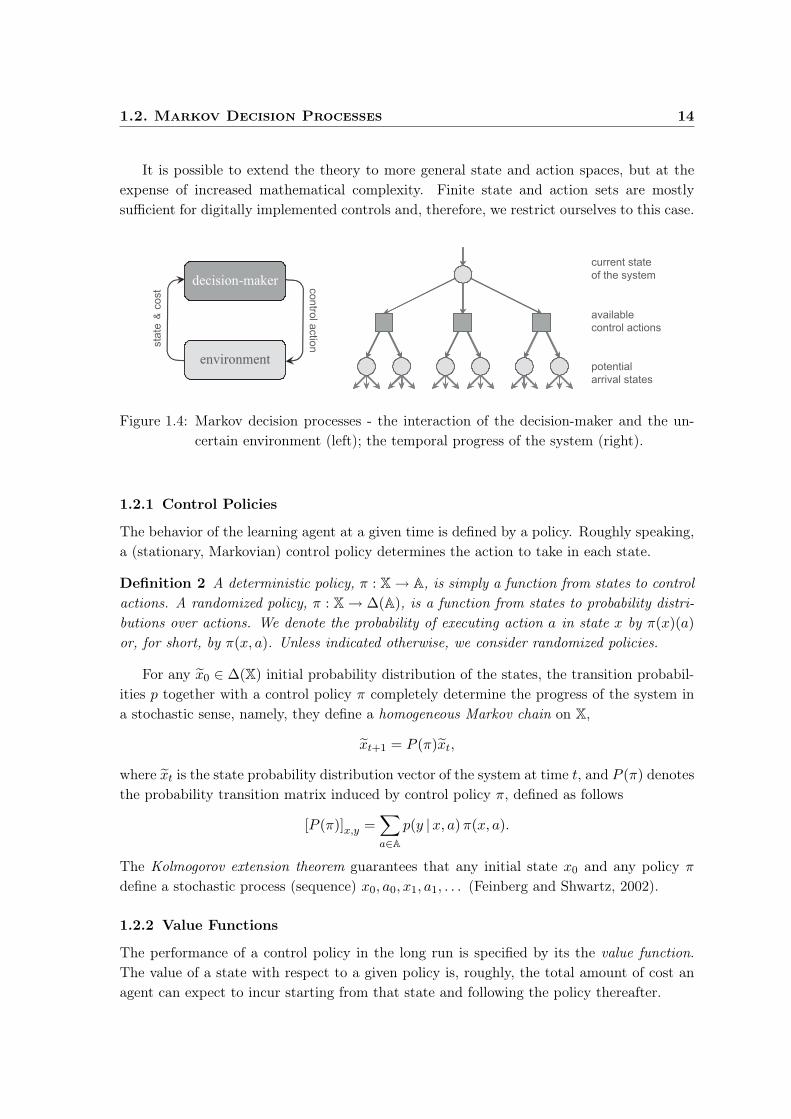
An interpretation of an MDP can be given, which viewpoint is often taken in RL, if weconsider an agent that acts in an uncertain environment. The agent receives informationabout the state of the environment, x, at each state x the agent is allowed to choose anaction a ∈ A(x). After the action is selected, the environment moves to the next stateaccording to the probability distribution p(x, a) and the decision-maker collects its one-stepcost, g(x, a). The aim of the agent is to find an optimal behavior (policy), such that applyingthis strategy minimizes the expected cumulative costs over a finite or infinite horizon.
A stochastic shortest path (SSP) problem is a special MDP in which the aim is to finda control policy such that reaches a pre-defined terminal state starting from a given initialstate, additionally, minimizes the expected total costs of the path, as well. A policy iscalled proper if it reaches the terminal state with probability one. A usual assumption whendealing with SSP problems is that all policies are proper, which is abbreviated as APP.
1.2. Markov Decision Processes 14
It is possible to extend the theory to more general state and action spaces, but at theexpense of increased mathematical complexity. Finite state and action sets are mostlysufficient for digitally implemented controls and, therefore, we restrict ourselves to this case.
Figure 1.4: Markov decision processes - the interaction of the decision-maker and the un-certain environment (left); the temporal progress of the system (right).
1.2.1 Control Policies
The behavior of the learning agent at a given time is defined by a policy. Roughly speaking,a (stationary, Markovian) control policy determines the action to take in each state.
Definition 2 A deterministic policy, π : X → A, is simply a function from states to control
actions. A randomized policy, π : X → ∆(A), is a function from states to probability distri-
butions over actions. We denote the probability of executing action a in state x by π(x)(a)
or, for short, by π(x, a). Unless indicated otherwise, we consider randomized policies.
For any x0 ∈ ∆(X) initial probability distribution of the states, the transition probabil-ities p together with a control policy π completely determine the progress of the system ina stochastic sense, namely, they define a homogeneous Markov chain on X,
xt+1 = P (π)xt,
where xt is the state probability distribution vector of the system at time t, and P (π) denotesthe probability transition matrix induced by control policy π, defined as follows
[P (π)]x,y =∑
a∈A
p(y |x, a)π(x, a).
The Kolmogorov extension theorem guarantees that any initial state x0 and any policy π
define a stochastic process (sequence) x0, a0, x1, a1, . . . (Feinberg and Shwartz, 2002).
1.2.2 Value Functions
The performance of a control policy in the long run is specified by its the value function.The value of a state with respect to a given policy is, roughly, the total amount of cost anagent can expect to incur starting from that state and following the policy thereafter.
1.2. Markov Decision Processes 15
Definition 3 The value or cost-to-go function of a policy π is a function from states to
costs, Jπ : X → R. Function Jπ(x) gives the expected value of the cumulative (discounted)
costs when the system is in state x and it follows policy π thereafter,
Jπ(x) = E
[N∑
t=0
αtg(Xt, Aπt )
∣∣∣∣ X0 = x
], (1.1)
where Xt and Aπt are random variables, Aπ
t is selected according to control policy π and the
distribution of Xt+1 is p(Xt, Aπt ). The horizon of the problem is denoted by N ∈ N ∪ ∞.
Unless indicated otherwise, we will always assume that the horizon is infinite, N = ∞.
Similarly to the definition of Jπ, one can define action-value functions of control polices,
Qπ(x, a) = E
[N∑
t=0
αtg(Xt, Aπt )
∣∣∣∣ X0 = x,Aπ0 = a
],
where the notations are the same as in equation (1.1). Action-value functions are especiallyimportant for model-free approaches, such as the classical Q-learning algorithm.
1.2.3 Bellman Equations
We saw that the agent aims at finding an optimal policy which minimizes the expected costs.In order to define optimal solutions, we also need a concept for comparing policies.
Definition 4 We say that π1 ≤ π2 if and only if ∀x ∈ X : Jπ1(x) ≤ Jπ2(x). A control
policy is (uniformly) optimal if it is less than or equal to all other control policies.
There always exists at least one optimal policy (Sutton and Barto, 1998). Although theremay be many optimal policies, they all share the same unique optimal cost-to-go function,denoted by J∗. This function must satisfy the Bellman optimality equation, TJ∗ = J∗,where T is the Bellman operator (Bertsekas and Tsitsiklis, 1996), defined for all x ∈ X, as
(TJ)(x) = mina∈A(x)
[g(x, a) + α
∑
y∈X
p(y |x, a)J(y)]. (1.2)
The Bellman equation for an arbitrary (stationary, Markovian, randomized) policy is
(T πJ)(x) =∑
a∈A(x)
π(x, a)[g(x, a) + α
∑
y∈X
p(y |x, a)J(y)],
where the notations are the same as in equation (1.2) and we also have T πJπ = Jπ.
Definition 5 We say that function f : X → Y, where X , Y are normed spaces, is Lipschitz
continuous if there exists a β ≥ 0 such that ∀x1, x2 ∈ X : ‖f(x1) − f(x2)‖Y ≤ β ‖x1 − x2‖X ,
where ‖·‖X and ‖·‖Y denote the norm of X and Y, respectively. The smallest such β is called
the Lipschitz constant of f . Henceforth, assume that X = Y. If the Lipschitz constant β < 1,
then the function is called a contraction. A mapping is called a pseudo-contraction if there
exists an x∗ ∈ X and a β ≥ 0 such that ∀x ∈ X , we have ‖f(x) − x∗‖X ≤ β ‖x− x∗‖X .
1.2. Markov Decision Processes 16
Naturally, every contraction mapping is also a pseudo-contraction, however, the oppositeis not true. The pseudo-contraction condition implies that x∗ is the fixed point of functionf , namely, f(x∗) = x∗, moreover, x∗ is unique, thus, f cannot have other fixed points.
It is known that the Bellman operator is a supremum norm contraction with Lipschitzconstant α. In case we consider stochastic shortest path (SSP) problems, which arise ifthe MDP has an absorbing terminal (goal) state, then the Bellman operator becomes apseudo-contraction in the weighted supremum norm (Bertsekas and Tsitsiklis, 1996).
1.2.4 Approximate Solutions
From a given value function J , it is straightforward to get a policy, e.g., by applying a greedy
and deterministic policy (w.r.t. J) that always selects actions with minimal costs,
π(x) ∈ arg mina∈A(x)
[g(x, a) + α
∑
y∈X
p(y |x, a)J(y)].
MDPs have an extensively studied theory and there exist a lot of exact and approximatesolution methods, e.g., value iteration, policy iteration, the Gauss-Seidel method, Q-learning,Q(λ), SARSA and TD(λ) - temporal difference learning (Bertsekas and Tsitsiklis, 1996;Sutton and Barto, 1998; Feinberg and Shwartz, 2002). Most of these reinforcement learningalgorithms work by iteratively approximating the optimal value function.
If J is “close” to J∗, then the greedy policy with one-stage lookahead based on J willalso be “close” to an optimal policy, as it was proven by Bertsekas and Tsitsiklis (1996):
Theorem 6 Let M be a discounted MDP and J is an arbitrary value function. The value
function of the greedy policy based on J is denoted by Jπ. Then, we have
‖Jπ − J∗‖∞ ≤2α
1 − α‖J − J∗‖∞ ,
where ‖·‖∞ denotes the supremum norm, more precisely, ‖f‖∞ = sup |f(x)| : x ∈ dom(f).
Moreover, there exists an ε > 0 such that if ‖J − J∗‖∞ < ε, then J∗ = Jπ.
Consequently, if we could obtain a good approximation of the optimal value function,then we immediately had a good control policy, as well, e.g., the greedy policy with respectto our approximate value function. Therefore, the main question for most RL approaches isthat how a good approximation to the optimal value function could be achieved.
1.2.5 Partial Observability
In an MDP it is assumed that the agent is perfectly informed about the current state ofthe environment, which presupposition is often unrealistic. In partially observable Markov
decision processes (POMDPs), which are well-known generalizations of MDPs, the decision-maker does not necessarily know the precise state of the environment: some observations areavailable to ground the decision upon, however, these information can be partial and noisy.Formally, a POMDP has all components of a (fully observable) MDP and, additionally, it hasa finite observation set O and a function for the observation probabilities q : X×A → ∆(O).

1.2. Markov Decision Processes 17
The notation p(z | x, a) shows the probability that the decision-maker receives observation zafter executing action a in state x. Note that in POMDPs the availability function dependson the observations rather than the real states of the underlying MDP, A : O → P(A).
Control policies of POMDPs are also defined on observations. Thus, a (non-Markovian)deterministic policy takes the form of π : O∗ → A, where O∗ denotes the set of all finitesequences over O. Respectively, randomized policies are defined as π : O∗ → ∆(A).
An important idea in the theory of POMDPs is the concept of belief states, which areprobability distributions over the states of the environment. They were suggested by Åström(1965) and they can be interpreted as the decision-maker’s ideas about the current state.We denote the belief space by B = ∆(X). The belief state is a sufficient statistic in thesense that the agent can perform as well based upon belief states as if it had access tothe whole history of observations (Smallwood and Sondik, 1973). Therefore, a Markoviancontrol policy based on belief states, πb : B → ∆(A), as it was shown, can be as efficient asa non-Markovian control policy that applies all past observations, πo : O∗ → ∆(A).
Given a belief state b, a control action a and an observation z, the successor belief stateτ(b, a, z) ∈ B can be calculated by the Bayes rule, more precisely, as follows
τ(b, a, z)(y) =
∑x∈X
p(z, y | x, a) b(x)
p(z | b, a),
where p(z, y | x, a) = p(z | y, a) · p(y | x, a) and p(z | b, a) can be computed by
p(z | b, a) =∑
x,y∈X
p(z, y | x, a) b(x) .
It is known (Aberdeen, 2003) that with the concept of belief states, a POMDP can betransformed into a fully observable MDP. The resulting process is called the belief state
MDP. The state space of the belief state MDP is B, its action space is A, and the transition-probabilities from any state b1 to state b2 after executing action a can be determined by
p(b2 | b1, a) =
p(z | b1, a) if b2 = τ(b1, a, z) for some z
0 otherwise
The immediate-cost function of the belief state MDP for all b ∈ B, a ∈ A is given by
g(b, a) =∑
x∈X
b(x) g(x, a),
consequently, the optimal cost-to-go function of the belief state MDP, denoted by J∗, is
J∗(b) = mina∈A(b)
[g(b, a) + α
∑
z∈O
p(z | b, a) J∗(τ(b, a, z))].
Due to this reformulation, solving a POMDP, in theory, can be accomplished by solving thecorresponding belief state MDP. However, usually it is hard to translate this approach intoefficient solution methods. Some approximate solutions are considered by Aberdeen (2003).
1.3. Main Contributions 18
1.3 Main Contributions
The main contributions and the new scientific results of the dissertation can be summarizedin six points which can be organized in two thesis groups. The first group concerns withefficiently solving RAPs in presence of uncertainties, while the second contains results onmanaging changes in the environmental dynamics. It is expected to formulate the contribu-tions in first-person singular form, in order to express that they are my own results.
1.3.1 Stochastic Resource Allocation
In Chapter 2 I study RAPs in presence of uncertainties. I also suggest machine learningbased solution methods to handle them. My main contributions are as follows:
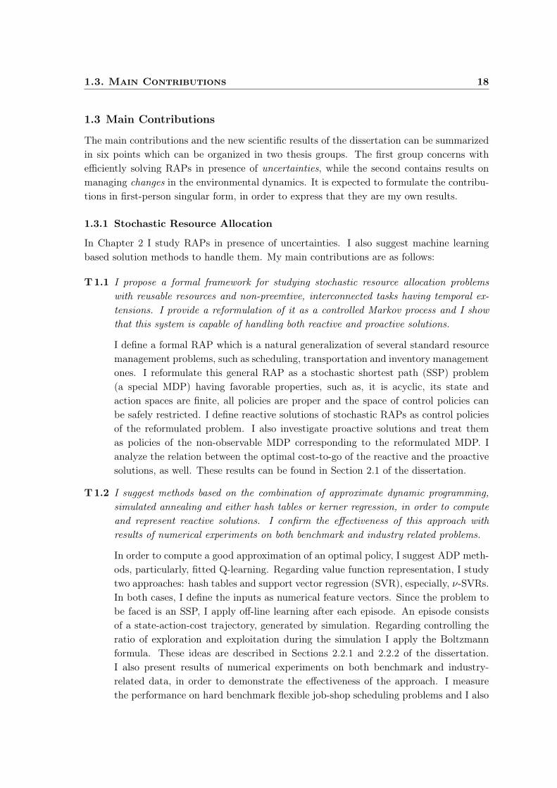
T1.1 I propose a formal framework for studying stochastic resource allocation problems
with reusable resources and non-preemtive, interconnected tasks having temporal ex-
tensions. I provide a reformulation of it as a controlled Markov process and I show
that this system is capable of handling both reactive and proactive solutions.
I define a formal RAP which is a natural generalization of several standard resourcemanagement problems, such as scheduling, transportation and inventory managementones. I reformulate this general RAP as a stochastic shortest path (SSP) problem(a special MDP) having favorable properties, such as, it is acyclic, its state andaction spaces are finite, all policies are proper and the space of control policies canbe safely restricted. I define reactive solutions of stochastic RAPs as control policiesof the reformulated problem. I also investigate proactive solutions and treat themas policies of the non-observable MDP corresponding to the reformulated MDP. Ianalyze the relation between the optimal cost-to-go of the reactive and the proactivesolutions, as well. These results can be found in Section 2.1 of the dissertation.
T1.2 I suggest methods based on the combination of approximate dynamic programming,
simulated annealing and either hash tables or kerner regression, in order to compute
and represent reactive solutions. I confirm the effectiveness of this approach with
results of numerical experiments on both benchmark and industry related problems.
In order to compute a good approximation of an optimal policy, I suggest ADP meth-ods, particularly, fitted Q-learning. Regarding value function representation, I studytwo approaches: hash tables and support vector regression (SVR), especially, ν-SVRs.In both cases, I define the inputs as numerical feature vectors. Since the problem tobe faced is an SSP, I apply off-line learning after each episode. An episode consistsof a state-action-cost trajectory, generated by simulation. Regarding controlling theratio of exploration and exploitation during the simulation I apply the Boltzmannformula. These ideas are described in Sections 2.2.1 and 2.2.2 of the dissertation.I also present results of numerical experiments on both benchmark and industry-related data, in order to demonstrate the effectiveness of the approach. I measurethe performance on hard benchmark flexible job-shop scheduling problems and I also
1.3. Main Contributions 19
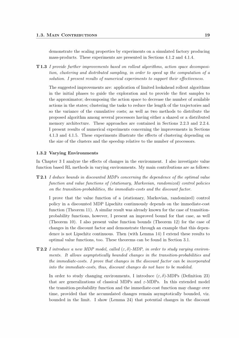
demonstrate the scaling properties by experiments on a simulated factory producingmass-products. These experiments are presented in Sections 4.1.2 and 4.1.4.
T1.3 I provide further improvements based on rollout algorithms, action space decomposi-
tion, clustering and distributed sampling, in order to speed up the computation of a
solution. I present results of numerical experiments to support their effectiveness.
The suggested improvements are: application of limited lookahead rollout algorithmsin the initial phases to guide the exploration and to provide the first samples tothe approximator; decomposing the action space to decrease the number of availableactions in the states; clustering the tasks to reduce the length of the trajectories andso the variance of the cumulative costs; as well as two methods to distribute theproposed algorithm among several processors having either a shared or a distributedmemory architecture. These approaches are contained in Sections 2.2.3 and 2.2.4.I present results of numerical experiments concerning the improvements in Sections4.1.3 and 4.1.5. These experiments illustrate the effects of clustering depending onthe size of the clusters and the speedup relative to the number of processors.
1.3.2 Varying Environments
In Chapter 3 I analyze the effects of changes in the environment. I also investigate valuefunction based RL methods in varying environments. My main contributions are as follows:
T2.1 I deduce bounds in discounted MDPs concerning the dependence of the optimal value
function and value functions of (stationary, Markovian, randomized) control policies
on the transition-probabilities, the immediate-costs and the discount factor.
I prove that the value function of a (stationary, Markovian, randomized) controlpolicy in a discounted MDP Lipschitz continuously depends on the immediate-costfunction (Theorem 11). A similar result was already known for the case of transition-probability functions, however, I present an improved bound for that case, as well(Theorem 10). I also present value function bounds (Theorem 12) for the case ofchanges in the discount factor and demonstrate through an example that this depen-dence is not Lipschitz continuous. Then (with Lemma 14) I extend these results tooptimal value functions, too. These theorems can be found in Section 3.1.
T2.2 I introduce a new MDP model, called (ε, δ)-MDP, in order to study varying environ-
ments. It allows asymptotically bounded changes in the transition-probabilities and
the immediate-costs. I prove that changes in the discount factor can be incorporated
into the immediate-costs, thus, discount changes do not have to be modeled.
In order to study changing environments, I introduce (ε, δ)-MDPs (Definition 23)that are generalizations of classical MDPs and ε-MDPs. In this extended modelthe transition-probability function and the immediate-cost function may change overtime, provided that the accumulated changes remain asymptotically bounded, viz.bounded in the limit. I show (Lemma 24) that potential changes in the discount

1.3. Main Contributions 20
factor can be incorporated into the immediate-cost function, thus, discount changesdo not have to be considered. These contributions are presented in Section 3.2.2.
T2.3 I prove a general convergence theorem for time-dependent stochastic iterative algo-
rithms. As a corollary, I deduce an approximation theorem for value function based
reinforcement learning (RL) methods working in (ε, δ)-MDPs. I also illustrate these
results through three classical RL algorithms as well as numerical experiments.
I analyze stochastic iterative algorithms where the value function update operatormay change over time. I prove a relaxed convergence theorem for this kind of al-gorithm (Theorem 26). As a corollary, I get an approximation theorem for valuefunction based RL methods working in (ε, δ)-MDPs (Corollary 27). Furthermore, Iillustrate my results through three classical RL algorithms. I deduce relaxed con-vergence properties in (ε, δ)-MDPs for asynchronous value iteration, Q-learning andTD(λ) – temporal difference learning. In order to demonstrate the results, I presenttwo simple stochastic iterative algorithms, a “well-behaving” and a “pathological”one. These contributions are described in Sections 3.2.3 and 3.2.4. I also presentresults of numerical experiments which highlight some features of working in varyingenvironments. I show two experiments concerning adaptation in Section 4.2.

Chapter 2
Stochastic Resource Allocation
As we saw in Chapter 1, resource allocation problems (RAPs) have may important practicalapplications and, usually, they are difficult to solve, even in deterministic cases. It is known,for example, that both JSP and TSP are strongly NP-hard, moreover, they do not haveany good polynomial time approximation algorithm, either. Additionally, in “real world”problems we often have to face uncertainties, e.g., in many cases the processing times of thetasks or the durations of the trips are not known exactly in advance, only estimations areavailable to work with, e.g., these values are given by suitable random variables.
Unfortunately, it is not trivial to extend classical approaches, such as branch and cut orconstraint satisfaction algorithms, to handle stochastic RAPs. Simply replacing the randomvariables with their expected values and, then, applying standard deterministic algorithms,usually, does not lead to efficient solutions. The issue of additional uncertainties in RAPsmakes them even more challenging and call for advanced techniques. In the dissertation wesuggest applying statistical machine learning (ML) methods to handle these problems.
In this chapter, first, we define a general resource allocation framework which is a naturalextension of several standard resource management problems, such as JSP and TSP. Then,in order to apply ML methods, we reformulate it as an MDP. Both proactive (off-line) andreactive (on-line) resource allocation are considered and their relation is analyzed. Con-cerning efficient solution methods, we restrict ourselves to reactive solutions. We suggestregression based RL methods to solve RAPs and, later, we extend the solution with severaladditional improvements to speed up the computation of an efficient control policy.
2.1 Markovian Resource Control
This section aims at precisely defining RAPs and reformulating them in a way that theycould be effectively solved by machine learning methods presented in Section 2.2. First, ageneral resource allocation framework is described. We start with deterministic variants andthen extend the definition to the stochastic case. Afterwards, we reformulate the reactiveproblem as an MDP. Later, with the help of POMDPS, we study how this approach could beextended to proactive solutions. Finally, we show that the solution of the proactive problemcan be lower and upper bounded with the help of the corresponding reactive solution.
21

2.1. Markovian Resource Control 22
2.1.1 Deterministic Framework
Now, we present a general formal framework to model diverse resource allocation problems.As we will see, this framework is an extension of several classical combinatorial optimizationtype RAPs, such as scheduling and transportation problems, e.g., JSP and TSP.
First, a deterministic resource allocation problem is considered: an instance of the prob-lem can be characterized by an 8-tuple 〈R,S,O, T , C, d, e, i〉. In details the problem consistsof a set of reusable resources R together with S that corresponds to the set of possible re-
source states. A set of allowed operations O is also given with a subset T ⊆ O which denotesthe target operations or tasks. R, S and O are supposed to be finite and they are pairwisedisjoint. There can be precedence constrains between the tasks, which are represented by apartial ordering C ⊆ T × T . The durations of the operations depending on the state of theexecuting resource are defined by a partial function d : S × O → N, where N is the set ofnatural numbers, thus, we have a discrete-time model. Every operation can affect the stateof the executing resource, as well, that is described by e : S ×O → S which is also a partialfunction. It is assumed that dom(d) = dom(e), where dom(·) denotes the domain set of afunction. Finally, the initial states of the resources are given by i : R → S.
The state of a resource can contain all relevant information about it, for example, its typeand current setup (scheduling problems), its location and load (transportation problems) orcondition (maintenance and repair problems). Similarly, an operation can affect the statein many ways, e.g., it can change the setup of the resource, its location or condition. Thesystem must allocate each task (target operation) to a resource, however, there may be caseswhen first the state of a resource must be modified in order to be able to execute a certaintask (e.g., a transporter may need, first, to travel to its loading/source point, a machinemay require repair or setup). In these cases non-task operations may be applied. They canmodify the states of the resources without directly serving a demand (executing a task). Itis possible that during the resource allocation process a non-task operation is applied severaltimes, but other non-task operations are completely avoided (for example, because of theirhigh cost). Nevertheless, finally, all tasks must be completed.
Feasible Resource Allocation
A solution for a deterministic RAP is a partial function, the resource allocator function,% : R×N → O that assigns the starting times of the operations on the resources. Note thatthe operations are supposed to be non-preemptive (they may not be interrupted).
A solution is called feasible if and only if the following four properties are satisfied:
1. All tasks are associated with exactly one (resource, time point) pair:∀v ∈ T : ∃! 〈r, t〉 ∈ dom(%) : v = %(r, t).
2. Each resource executes, at most, one operation at a time:¬∃u, v ∈ O : u = %(r, t1) ∧ v = %(r, t2) ∧ t1 ≤ t2 < t1 + d(s(r, t1), u).
3. The precedence constraints of the tasks are kept:∀ 〈u, v〉 ∈ C : [u = %(r1, t1) ∧ v = %(r2, t2)] ⇒ [t1 + d(s(r1, t1), u) ≤ t2] .
2.1. Markovian Resource Control 23
4. Every operation-to-resource assignment is valid:∀ 〈r, t〉 ∈ dom(%) : 〈s(r, t), %(r, t)〉 ∈ dom(d),
where s : R× N → S describes the states of the resources at given times
s(r, t) =
i(r) if t = 0
s(r, t− 1) if 〈r, t〉 /∈ dom(%)
e(s(r, t− 1), %(r, t)) otherwise
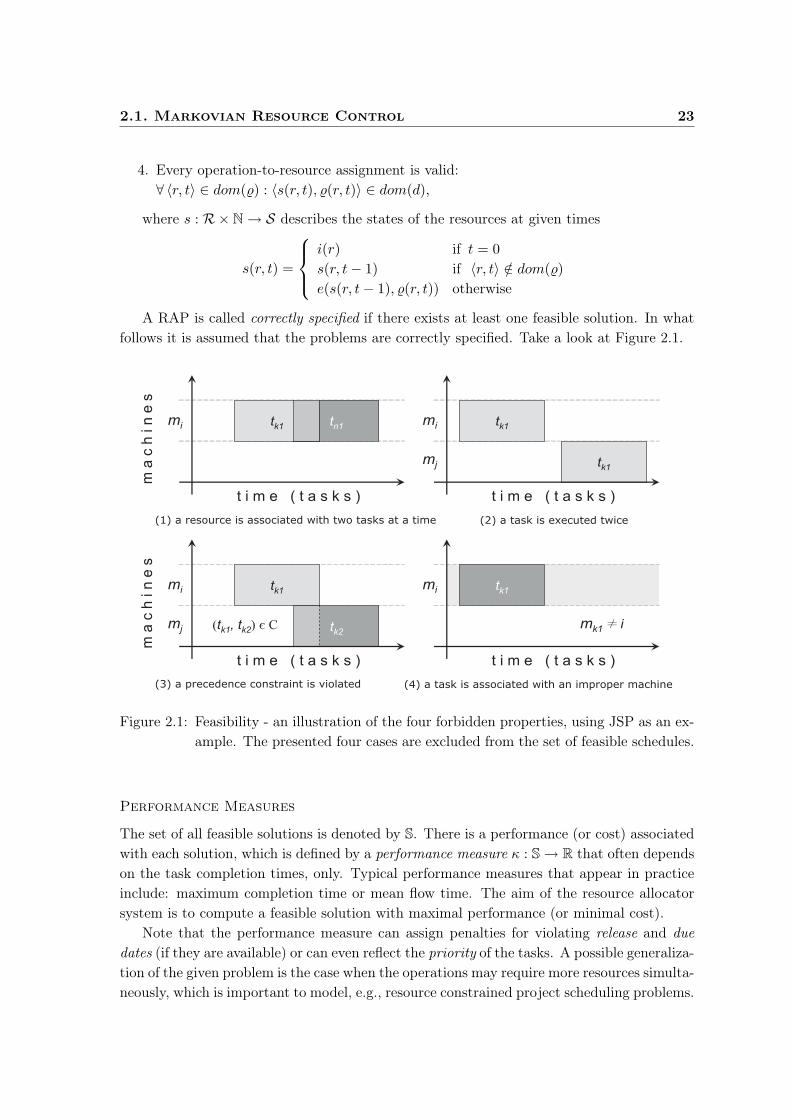
A RAP is called correctly specified if there exists at least one feasible solution. In whatfollows it is assumed that the problems are correctly specified. Take a look at Figure 2.1.
Figure 2.1: Feasibility - an illustration of the four forbidden properties, using JSP as an ex-ample. The presented four cases are excluded from the set of feasible schedules.
Performance Measures
The set of all feasible solutions is denoted by S. There is a performance (or cost) associatedwith each solution, which is defined by a performance measure κ : S → R that often dependson the task completion times, only. Typical performance measures that appear in practiceinclude: maximum completion time or mean flow time. The aim of the resource allocatorsystem is to compute a feasible solution with maximal performance (or minimal cost).
Note that the performance measure can assign penalties for violating release and due
dates (if they are available) or can even reflect the priority of the tasks. A possible generaliza-tion of the given problem is the case when the operations may require more resources simulta-neously, which is important to model, e.g., resource constrained project scheduling problems.

2.1. Markovian Resource Control 24
However, it is straightforward to extend the framework to this case: the definition of d ande should be changed to d : S〈k〉 × O → N and e : S〈k〉 × O → S〈k〉, where S〈k〉 = ∪k
i=1Si
and k ≤ |R|. Naturally, we assume that for all 〈s, o〉 ∈ dom(e) : dim(e(s, o)) = dim(s).Although, managing tasks with multiple resource requirements may be important in somecases, to keep the analysis as simple as possible, we do not include them in the model.Nevertheless, the presented model could be easily generalized to this case and, moreover,the solution methods presented in Section 2.2 are applicable to handle such tasks, as well.
Demonstrative Examples
Now, as demonstrative examples, we reformulate (F)JSP and TSP in the given framework.It is straightforward to formulate scheduling problems, such as JSP, in the presented
resource allocation framework: the tasks of JSP can be directly associated with the tasksof the framework, machines can be associated with resources and processing times withdurations. The precedence constraints are determined by the linear ordering of the tasksin each job. Note that there is only one possible resource state for every machine. Finally,feasible schedules can be associated with feasible solutions. If there were setup-times inthe problem, as well, then there would be several states for each resource (according to itscurrent setup) and the “set-up” procedures could be associated with the non-task operations.
Regarding the RAP formulation of TSP, R = r, where r corresponds to the “salesman”.S = s1, . . . , sn, if the state (of r) is si, it indicates that the salesman is in city i. O =
T = t1, . . . , tn, where the execution of task ti symbolizes that the salesman goes to cityi from his current location. The constraints C = 〈t2, t1〉 , 〈t3, t1〉 . . . , 〈tn, t1〉 are used forforcing the system to end the whole round-tour in city 1, which is also the starting city,thus, i(r) = s1. For all si ∈ S and tj ∈ T : 〈si, tj〉 ∈ dom(d) if and only if 〈i, j〉 ∈ E. For all〈si, tj〉 ∈ dom(d) : d(si, tj) = wij and e(si, tj) = sj . Note that dom(e) = dom(d) and the firstfeasibility requirement guarantees that each city is visited exactly once. The performancemeasure κ is the latest arrival time, κ(%) = max t+ d(s(r, t), %(r, t)) | 〈r, t〉 ∈ dom(%).
Computational Complexity
If we use a performance measure which has the property that a solution can be preciselydefined by a bounded sequence of operations (which includes all tasks) with their assignmentto the resources and, additionally, among the solutions generated this way an optimal one canbe found, then the RAP becomes a combinatorial optimization problem. Each performancemeasure monotone in the completion times, these measures are called regular, has thisproperty. Because the above defined RAP is a generalization of, e.g., JSP and TSP, it isstrongly NP-hard and, furthermore, no good polynomial-time approximation of the optimalresource allocating algorithm exists, either (Papadimitriou, 1994).
2.1.2 Stochastic Framework
So far our model has been deterministic, now we turn to stochastic RAPs. The stochasticvariant of the described general class of RAPs can be defined by randomizing functions d,
2.1. Markovian Resource Control 25
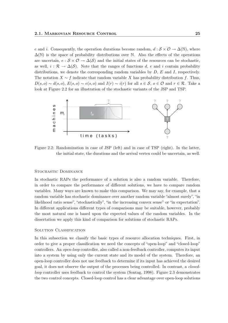
e and i. Consequently, the operation durations become random, d : S × O → ∆(N), where∆(N) is the space of probability distributions over N. Also the effects of the operationsare uncertain, e : S × O → ∆(S) and the initial states of the resources can be stochastic,as well, i : R → ∆(S). Note that the ranges of functions d, e and i contain probabilitydistributions, we denote the corresponding random variables by D, E and I, respectively.The notation X ∼ f indicate that random variable X has probability distribution f . Thus,D(s, o) ∼ d(s, o), E(s, o) ∼ e(s, o) and I(r) ∼ i(r) for all s ∈ S, o ∈ O and r ∈ R. Take alook at Figure 2.2 for an illustration of the stochastic variants of the JSP and TSP.
Figure 2.2: Randomization in case of JSP (left) and in case of TSP (right). In the latter,the initial state, the durations and the arrival vertex could be uncertain, as well.
Stochastic Dominance
In stochastic RAPs the performance of a solution is also a random variable. Therefore,in order to compare the performance of different solutions, we have to compare randomvariables. Many ways are known to make this comparison. We may say, for example, that arandom variable has stochastic dominance over another random variable “almost surely”, “inlikelihood ratio sense”, “stochastically”, “in the increasing convex sense” or “in expectation”.In different applications different types of comparisons may be suitable, however, probablythe most natural one is based upon the expected values of the random variables. In thedissertation we apply this kind of comparison for solutions of stochastic RAPs.
Solution Classification
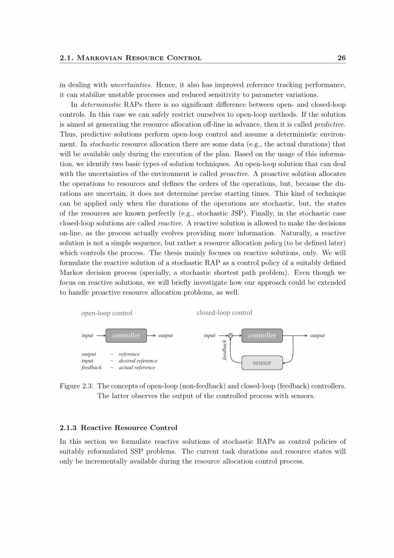
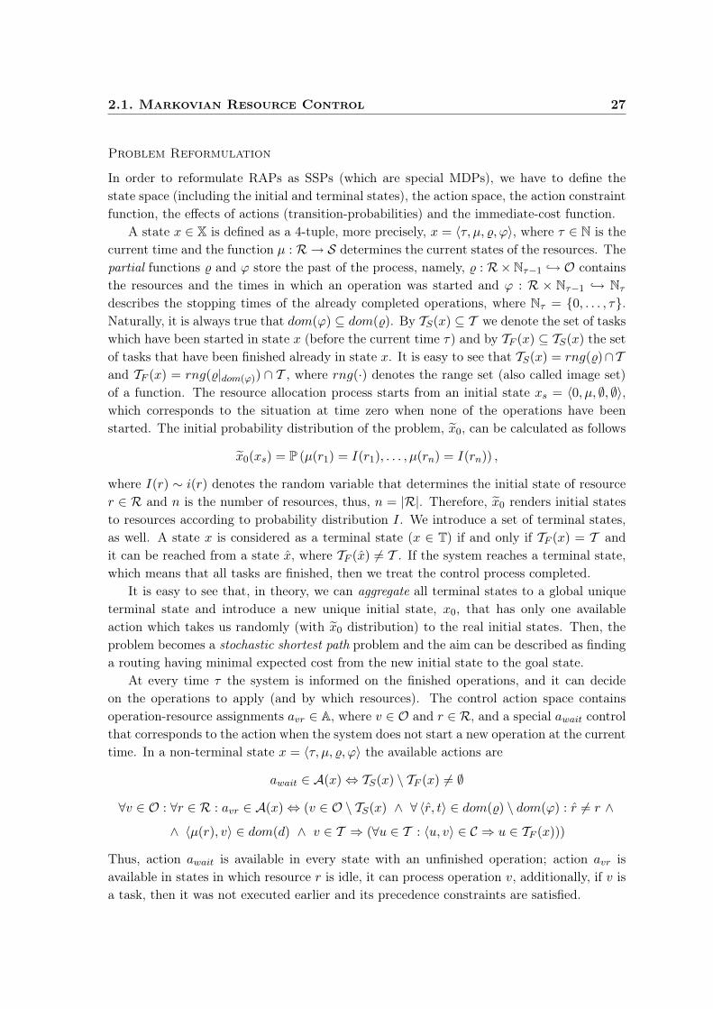
In this subsection we classify the basic types of resource allocation techniques. First, inorder to give a proper classification we need the concepts of “open-loop” and “closed-loop”controllers. An open-loop controller, also called a non-feedback controller, computes its inputinto a system by using only the current state and its model of the system. Therefore, anopen-loop controller does not use feedback to determine if its input has achieved the desiredgoal, it does not observe the output of the processes being controlled. In contrast, a closed-
loop controller uses feedback to control the system (Sontag, 1998). Figure 2.3 demonstratesthe two control concepts. Closed-loop control has a clear advantage over open-loop solutions
2.1. Markovian Resource Control 26
in dealing with uncertainties. Hence, it also has improved reference tracking performance,it can stabilize unstable processes and reduced sensitivity to parameter variations.
In deterministic RAPs there is no significant difference between open- and closed-loopcontrols. In this case we can safely restrict ourselves to open-loop methods. If the solutionis aimed at generating the resource allocation off-line in advance, then it is called predictive.Thus, predictive solutions perform open-loop control and assume a deterministic environ-ment. In stochastic resource allocation there are some data (e.g., the actual durations) thatwill be available only during the execution of the plan. Based on the usage of this informa-tion, we identify two basic types of solution techniques. An open-loop solution that can dealwith the uncertainties of the environment is called proactive. A proactive solution allocatesthe operations to resources and defines the orders of the operations, but, because the du-rations are uncertain, it does not determine precise starting times. This kind of techniquecan be applied only when the durations of the operations are stochastic, but, the statesof the resources are known perfectly (e.g., stochastic JSP). Finally, in the stochastic caseclosed-loop solutions are called reactive. A reactive solution is allowed to make the decisionson-line, as the process actually evolves providing more information. Naturally, a reactivesolution is not a simple sequence, but rather a resource allocation policy (to be defined later)which controls the process. The thesis mainly focuses on reactive solutions, only. We willformulate the reactive solution of a stochastic RAP as a control policy of a suitably definedMarkov decision process (specially, a stochastic shortest path problem). Even though wefocus on reactive solutions, we will briefly investigate how our approach could be extendedto handle proactive resource allocation problems, as well.
Figure 2.3: The concepts of open-loop (non-feedback) and closed-loop (feedback) controllers.The latter observes the output of the controlled process with sensors.
2.1.3 Reactive Resource Control
In this section we formulate reactive solutions of stochastic RAPs as control policies ofsuitably reformulated SSP problems. The current task durations and resource states willonly be incrementally available during the resource allocation control process.
2.1. Markovian Resource Control 27
Problem Reformulation
In order to reformulate RAPs as SSPs (which are special MDPs), we have to define thestate space (including the initial and terminal states), the action space, the action constraintfunction, the effects of actions (transition-probabilities) and the immediate-cost function.
A state x ∈ X is defined as a 4-tuple, more precisely, x = 〈τ, µ, %, ϕ〉, where τ ∈ N is thecurrent time and the function µ : R → S determines the current states of the resources. Thepartial functions % and ϕ store the past of the process, namely, % : R× Nτ−1 → O containsthe resources and the times in which an operation was started and ϕ : R × Nτ−1 → Nτ
describes the stopping times of the already completed operations, where Nτ = 0, . . . , τ.Naturally, it is always true that dom(ϕ) ⊆ dom(%). By TS(x) ⊆ T we denote the set of taskswhich have been started in state x (before the current time τ) and by TF (x) ⊆ TS(x) the setof tasks that have been finished already in state x. It is easy to see that TS(x) = rng(%)∩T
and TF (x) = rng(%|dom(ϕ)) ∩ T , where rng(·) denotes the range set (also called image set)of a function. The resource allocation process starts from an initial state xs = 〈0, µ, ∅, ∅〉,which corresponds to the situation at time zero when none of the operations have beenstarted. The initial probability distribution of the problem, x0, can be calculated as follows
x0(xs) = P (µ(r1) = I(r1), . . . , µ(rn) = I(rn)) ,
where I(r) ∼ i(r) denotes the random variable that determines the initial state of resourcer ∈ R and n is the number of resources, thus, n = |R|. Therefore, x0 renders initial statesto resources according to probability distribution I. We introduce a set of terminal states,as well. A state x is considered as a terminal state (x ∈ T) if and only if TF (x) = T andit can be reached from a state x, where TF (x) 6= T . If the system reaches a terminal state,which means that all tasks are finished, then we treat the control process completed.
It is easy to see that, in theory, we can aggregate all terminal states to a global uniqueterminal state and introduce a new unique initial state, x0, that has only one availableaction which takes us randomly (with x0 distribution) to the real initial states. Then, theproblem becomes a stochastic shortest path problem and the aim can be described as findinga routing having minimal expected cost from the new initial state to the goal state.
At every time τ the system is informed on the finished operations, and it can decideon the operations to apply (and by which resources). The control action space containsoperation-resource assignments avr ∈ A, where v ∈ O and r ∈ R, and a special await controlthat corresponds to the action when the system does not start a new operation at the currenttime. In a non-terminal state x = 〈τ, µ, %, ϕ〉 the available actions are
await ∈ A(x) ⇔ TS(x) \ TF (x) 6= ∅
∀v ∈ O : ∀r ∈ R : avr ∈ A(x) ⇔ (v ∈ O \ TS(x) ∧ ∀ 〈r, t〉 ∈ dom(%) \ dom(ϕ) : r 6= r ∧
∧ 〈µ(r), v〉 ∈ dom(d) ∧ v ∈ T ⇒ (∀u ∈ T : 〈u, v〉 ∈ C ⇒ u ∈ TF (x)))
Thus, action await is available in every state with an unfinished operation; action avr isavailable in states in which resource r is idle, it can process operation v, additionally, if v isa task, then it was not executed earlier and its precedence constraints are satisfied.

2.1. Markovian Resource Control 28
If an action avr ∈ A(x) is executed in a state x = 〈τ, µ, %, ϕ〉, then the system moveswith probability one to a new state x = 〈τ, µ, %, ϕ〉, where % = % ∪ 〈〈r, t〉 , v〉. Note thatwe treat functions as sets of ordered pairs. The resulting x corresponds to the state whereoperation v has started on resource r if the previous state of the environment was x.
The effect of the await action is that from x = 〈τ, µ, %, ϕ〉 it takes to an x = 〈τ + 1, µ, %, ϕ〉,where an unfinished operation %(r, t) that was started at t on r finishes with probability
P(〈r, t〉 ∈ dom(ϕ) | x, 〈r, t〉 ∈ dom(%) \ dom(ϕ)) =P(D(µ(r), %(r, t)) + t = τ)
P(D(µ(r), %(r, t)) + t ≥ τ),
where D(s, v) ∼ d(s, v) is a random variable that determines the duration of operation v
when it is executed by a resource which has state s. This quantity is called completion rate
in stochastic scheduling theory and hazard rate in reliability theory. We remark that foroperations with continuous durations, this quantity is defined by f(t)/(1 − F (t)), where fdenotes the density function and F the distribution of the random variable that determinesthe duration of the operation. If operation v = %(r, t) has finished (〈r, t〉 ∈ dom(ϕ)), thenϕ(r, t) = τ and µ(r) = E(r, v), where E(r, v) ∼ e(r, v) is a random variable that determinesthe new state of resource r after it has executed operation v. Except the extension of itsdomain set, the other values of function ϕ do not change, consequently, ∀ 〈r, t〉 ∈ dom(ϕ) :
ϕ(r, t) = ϕ(r, t). In other words, ϕ is a conservative extension of ϕ, formally, ϕ ⊆ ϕ.The cost function g, for a given κ performance measure (which depends only on the
operation-resource assignments and the completion times), is defined as follows. Let x =
〈τ, µ, %, ϕ〉 and x = 〈τ , µ, %, ϕ〉. Then, if the system arrives at state x after executing action ain state x, it incurs the cost κ(%, ϕ)−κ(%, ϕ). Note that, though, in Section 2.1.1 performancemeasures were defined on complete solutions, for most measures applied in practice (e.g.,makespan, weighted total lateness) it is straightforward to generalize the measure to partialsolutions, as well. One may, for example, treat the partial solution of a problem as a completesolution of a smaller (sub)problem, viz., a problem with fewer tasks.
Favorable Features
Let us call the introduced SSPs, which describe stochastic RAPs, RAP-MDPs. In thissection we overview some basic properties of RAP-MDPs. First, it is straightforward to seethat these MDPs have finite action spaces, since |A| ≤ |R| |O| + 1 always holds.
We may also observe that RAP-MDPs are acyclic, namely, none of the states can ap-pear multiple times, because during the resource allocation process τ and dom(%) are non-decreasing and, additionally, each time the state changes, the quantity τ + |dom(%)| strictlyincreases. Therefore, the system cannot reach the same state twice. As an immediate con-sequence, we can notice that all control policies eventually terminate and, therefore, proper.
Though, the state space of a RAP-MDP is denumerable in general, if the allowed num-ber of non-task operations is bounded and the random variables describing the operationdurations are finite, the state space of the reformulated MDP becomes finite, as well.
For the effective computation of a good control policy, it is important to try to reducethe number of states. We can do so by recognizing that if the performance measure κ is
2.1. Markovian Resource Control 29
non-decreasing in the completion times, then an optimal control policy of the reformulatedRAP-MDP can be found among the policies which start new operations only at times whenanother operation has been finished or in an initial state. This statement can be supportedby the fact that without increasing the cost (κ is non-decreasing) every operation can beshifted earlier on the resource which was assigned to it until it reaches another operation,or until it reaches a time when one of its preceding tasks is finished (if the operation wasa task with precedence constrains), or, ultimately, until time zero. Note that most of theperformance measures used in practice (e.g., makespan, weighted completion time, averagetardiness) are non-decreasing. As a consequence, the states in which no operation has beenfinished can be omitted, except the initial states. Therefore, each await action may lead toa state where an operation has been finished. We may consider it, as the system executesautomatically an await action in the omitted states. By this way, the state space can bedecreased and, therefore, a good control policy can be calculated more effectively.
Composable Measures
For a large class of performance measures, the state representation can be simplified byleaving out the past of the process. In order to do so, we must require that the performancemeasure be composable with a suitable function. In general, a function f : P(X) → R iscalled γ-composable if for any A,B ⊆ X, A∩B = ∅ it holds that γ(f(A), f(B)) = f(A∪B),where γ : R × R → R is called the composition function, and X is an arbitrary set. Thisdefinition can be directly applied to performance measures. If a performance measure, e.g.,is γ-composable, it indicates that the value of any complete solution can be computed fromthe values of its disjoint subsolutions (solutions to subproblems) with function γ. In practicalsituations the composition function is often the max, the min or the “+” function.
If the performance measure κ is γ-composable, then the past can be omitted from thestate representation, because the performance can be calculated incrementally. Thus, a statecan be described as x = 〈τ , κ, µ, TU 〉, where τ ∈ N, as previously, is the current time, κ ∈ R
contains the performance of the current (partial) solution and TU is the set of unfinishedtasks. The function µ : R → S×(O ∪ ι)×N determines the current states of the resourcestogether with the operations currently executed by them (or ι if a resource is idle) and thestarting times of the operations (needed to compute their completion rates).
In order to keep the analysis as simple as possible, we restrict ourselves to composablefunctions, since almost all performance measures that appear in practice are γ-composablefor a suitable γ (e.g., makespan or total production time is max-composable).
Reactive Solutions
Now, we are in a position to define the concept of reactive solutions for stochastic RAPs.A reactive solution is a (stationary, Markovian) control policy of the reformulated SSPproblem. It performs a closed-loop (on-line) control, since at each time step the controlleris informed about the current state of system and it can choose a control action based uponthis information. Section 2.2 deals with the computation of effective control policies.

2.1. Markovian Resource Control 30
2.1.4 Proactive Resource Control
In order to apply a reactive solution, which performs closed-loop control, sufficient feedbackshould be available from the system, e.g., provided by sensors. In some situations, however,we do not have such feedback and we must apply an open-loop controller, still, we shouldalso take uncertainties into account. In these cases one can design a proactive solution.Here, we suggest a way of extending our approach to be able to handle proactive problems.
The problem of proactive resource allocation can be formulated as a non-observable
Markov decision process (NOMDP) that is a special POMDP, in which the observation setcontains only one element, |O| = 1. In this case the equations describing the progress of thebelief state MDP can be simplified, e.g., the successor belief state can be computed by
τ(b, a)(y) =∑
x∈X
p(y | x, a) b(x),
where the observation parameter z is omitted, for obvious reasons. The Bellman equation,which describes the optimal cost-to-go function of the transformed MDP, is also simpler
J∗(b) = mina∈A
[g(b, a) + αJ∗(τ(b, a))
].
We argue that the already calculated reactive solution, namely, the cost-to-go functionof the fully observable MDP (FOMDP), J∗, can be used to accelerate the computationof finding a good policy for the proactive problem, since the cost-to-go function J∗ of theNOMDP can be lower and upper bounded by J∗. Computing a reactive solution is a mucheasier task than computing a proactive one, because, e.g., there are much fewer states tocount with, therefore, partially tracing back the problem of approximating the optimal cost-to-go of a NOMDP to the case of a FOMDP can mean a remarkable speedup. Moreover,the bounds are valid for arbitrary POMDPs, as well. Although, the first inequality ofthe presented statement follows from the results of Åström (1965), White (1976), or, morerecently, Hauskrecht (2000), we also present another direct proof of it in the appendix.
Theorem 7 Consider a POMDP and its fully observable MDP counterpart, which sys-
tem has the same state space, action space, transition-probabilities and costs as the original
POMDP, only the observability is different. The optimal cost-to-go functions of the POMDP
and the MDP are denoted by J∗ and J∗, respectively. Then, for all belief state b, we have
∑
x∈X
b(x)J∗(x) ≤ J∗(b) ≤∑
x∈X
b(x)J∗(x) +c
1 − α,
where c = (gmax − gmin); gmax = maxg(x, a) | x ∈ X, a ∈ A and similarly for gmin. If the
immediate-cost function g is not constant (c 6= 0), then the second inequality is strict.
The bounds for the optimal cost-to-go function of the belief state MDP are sharp, as thefollowing lemma shows (applying the usual notations for POMDPs and FOMDPs):
Lemma 8 (1) There exists a POMDP and a corresponding fully observable MDP such that,
for a belief state b: J∗(b) = 〈J∗, b〉; as well as (2) for all ε > 0 there exists a POMDP and
a corresponding MDP such that for a belief state b: |J∗(b) − 〈J∗, b〉 − c/(1 − α)| < ε.
2.2. Machine Learning Approaches 31
In this lemma 〈·, ·〉 denoted inner product, namely, 〈f, g〉 =∑
x f(x)g(x). If take a closerlook at the proof, located in the appendix, we can notice that the bounds remain sharp evenif we restrict ourselves to NOMDPs. The lower bound can be a remarkable help, e.g., whensuch an ADP method is applied that strictly requires non-underestimating initial values forthe approximated optimal cost-to-go function. An example of a learning method with suchassumption could be the real-time dynamic programming (RTDP) algorithm.
Proactive Solutions
As a summary, we can conclude that a proactive solution of a stochastic RAP is a (station-ary, Markovian) control policy of the corresponding NOMDP. It is known that POMDPscan be transformed into belief state MDPs, however, it is usually hard to translate thisresult into efficient practical solution algorithms. We have shown that the optimal solu-tion of the reactive problem can be applied to accelerate the calculation of the proactivesolution. Furthermore, there exists several approximation methods to ensure efficient so-lutions of POMDPs (Hauskrecht, 2000). In the thesis we present proactive solutions onlyas a possibility and leave their theoretical and practical investigations to further research.Henceforth, we will restrict ourselves to machine learning based reactive solutions.
2.2 Machine Learning Approaches
In this section we aim at giving an effective solution to large-scale RAPs in uncertain anddynamic environments with the help of different machine learning approaches. First, weoverview some reinforcement learning (RL) methods to compute a “good” policy. After-wards, we investigate two function approximation techniques to enhance the solution. Clus-tering, rollout algorithm and action decomposition as well as distributed sampling are alsoconsidered, as they can speedup the computation of a good control policy and, therefore,are important additions if we face large-scale problems. Later, in Chapter 3, we will see thatthis kind of approach can effectively work in changing environments, as well.
2.2.1 Reinforcement Learning
In the previous sections we have formulated RAPs as acyclic SSP problems. Now, we facethe challenge of finding a good policy. In theory, the optimal value function of a finiteMDP can be exactly computed by dynamic programming (DP) methods, such as valueiteration or the Gauss-Seidel method. Alternatively, an exact optimal policy can be directlycalculated by policy iteration. However, due to the “curse of dimensionality”, computingan exact optimal solution by these methods is practically infeasible, e.g., typically boththe required amount of computation and the needed storage space, viz., memory, growscombinatorially with the size of the problem. In order to handle the “curse”, we should applyapproximate dynamic programming (ADP) techniques to achieve a good approximation ofan optimal policy. Here, we suggest using sampling-based fitted Q-learning (FQL). In eachtrial a Monte-Carlo estimate of the value function is computed and projected onto a suitablefunction space. The methods described in this section (FQL, MCMC and the Boltzmann
2.2. Machine Learning Approaches 32
formula) should be applied simultaneously, in order to achieve an efficient solution. First,for the sake of better understandability, we overview two basic ADP methods which arecombined with function approximation: fitted value iteration and fitted policy iteration.
Fitted Value Iteration
The value iteration algorithm is one of the basic dynamic programming methods. It is definedby the iteration Jk+1 = TJk, where Jk is a value function and T is the Bellman operator,defined by equation (1.2). It is known that Jk converges in the supremum norm to J∗ forany initial J0, even if the updates of different states are performed asynchronously and alsofor more general operators (Bertsekas and Tsitsiklis, 1996; Szepesvári and Littman, 1999).The method of fitted value iteration (FVI) arises when the cost-to-go function is representedby a (typically parametric) function from a suitable function space F ⊆ J(X), where J(X)
denotes the space of value functions over X. In the case of finite MDPs, J(X) contains allJ : X → R functions. Thus, after each iteration the resulted value function is projected backonto F . Consequently, in general, the FVI algorithm proceeds as follows
Jk+1 ∈ arg minf∈F
‖f − TJk‖ ,
where ‖·‖ is an appropriate norm. FVI is a special case of approximate value iteration (AVI),where the updates follow the form Jk+1 = TJk + εk. Bertsekas and Tsitsiklis (1996) havepresented L∞ bounds for the convergence of AVI. Szepesvári and Munos (2005) have shownfinite time bounds for the convergence of FVI in case of weighted Lp norms.
Fitted Policy Iteration
There is an alternative to value iteration, called policy iteration, which always terminatesfinitely, in case of finite MDPs. Moreover, value iteration can be seen as a special case ofasynchronous policy iteration. In policy iteration, first, the policy is evaluated by applyingthe Bellman operator of policy π, then its is improved. It is known (Bertsekas and Tsitsiklis,1996) that iteration Jk+1 = T πJk converges to Jπ for any initial J0. Naturally, we do notneed to exactly compute Jπ. In asynchronous policy iteration, e.g., a subset of states Xk ⊆ X
is considered in iteration k and either value function Jk is updated according to
Jk+1(x) =
T πkJk(x) if x ∈ Xk
Jk(x) otherwise(2.1)
while leaving the policy unchanged, πk+1 = πk, or else the policy is improved, while thecost-to-go estimation remains the same, Jk+1 = Jk. The policy is updated as follows
πk+1(x) =
arg mina∈A(x)
[g(x, a) + α
∑y∈X
p(y | x, a)Jk(y)]
if x ∈ Xk
πk(x) otherwise(2.2)
where πk+1 : X → A is a deterministic policy, which is defined as greedy with respect toJk on Xk. It is known, e.g., (Bertsekas and Tsitsiklis, 1996), that if the value update (2.1)

2.2. Machine Learning Approaches 33
and the policy update (2.2) are executed infinitely often for all states and J0, π0 satisfyT π0J0 ≤ J0 then Jk converges in finitely many steps to the optimal cost-to-go, J∗. Thetechnique of asynchronous policy iteration can be interpreted as an actor-critic method.Similarly to FVI we can define fitted policy iteration by redefining the value update step as
Jk+1 ∈f ∈ F :
∥∥f − T πkJk
∥∥ ≤ ε,
where Tπkdenotes the operator that only updates the estimates of Xk according to T πk ,
viz., as defined by (2.1). Naturally, we should choose an ε such that ε > inff∈F∥∥f − T πkJk
∥∥or assume that F is dense in J(X). Note that if we assume that each value update step isautomatically followed by a policy update step (on the same states), then the actual controlpolicy does not need to be stored explicitly, it can be computed on-line, as needed.
Fitted Q-learning
Watkins’ Q-learning is a very popular off-policy, model-free reinforcement learning algorithm(Watkins, 1989; Watkins and Dayan, 1992; Even-Dar and Mansour, 2003). Q-learning ismodel-free, since it does not require a model of the environment, more precisely, it doesnot need the transition-probabilities and the immediate-costs, it satisfies with data comingfrom simulation. Moreover, Q-learning is off-policy, since it approximates the optimal valuefunction independently of the applied policy, as long as it makes sufficient explorations.
Q-learning works with action-value functions and iteratively approximates the optimalaction-value function, Q∗. The one-step (tabular) Q-learning rule is defined as follows
Qi+1(x, a) = (1 − γi(x, a))Qi(x, a) + γi(x, a)(TiQi)(x, a),
(TiQi)(x, a) = g(x, a) + α minB∈A(Y )
Qi(Y,B),
where γi(x, a) are the learning rates and Y is a random variable representing a state gen-erated from the pair (x, a) by simulation, that is, according to the probability distributionp(x, a). It is known (Bertsekas and Tsitsiklis, 1996) that if γi(x, a) ∈ [0, 1] and they satisfy
∞∑
i=0
γi(x, a) = ∞ and∞∑
i=0
γ2i (x, a) <∞,
then the Q-learning algorithm converges with probability one to the optimal action-valuefunction, Q∗, in the case of lookup table representation when each state-action value isstored independently. We speak about the method of fitted Q-learning (FQL) when thevalue function is represented by a (typically parametric) function from a suitable functionspace, F , and after each iteration, the updated value function is projected back onto F .
A useful observation is that we need the “learning rate” parameters only to overcome theeffects of random disturbances. However, if we deal with deterministic problems, this partof the method can be simplified. The resulting algorithm simply updates Q(x, a) with theminimum of the previously stored estimation and the current outcome of the simulation,which is also the core idea of the LRTA* algorithm (Bulitko and Lee, 2006). When we dealtwith deterministic resource allocation problems, we applied this simplification, as well.

2.2. Machine Learning Approaches 34
Evaluation by Simulation
Naturally, in large-scale problems we cannot update all states at once. Therefore, we performMarkov chain Monte Carlo (MCMC) simulations (Hastings, 1970; Andrieu et al., 2003) togenerate samples (with the model or with a simulator), which are used for computing the newapproximation of the estimated value function. Therefore, the set of states to be updatedin episode i, namely Xi, is generated by simulation. Because RAP-MDPs are acyclic, weapply prioritized sweeping, which means that after each iteration the cost-to-go estimationsare updated in the reverse order in which they appeared during the simulation. Assume, forexample, that Xi =
xi
1, xi2, . . . , x
iti
is the set of states for the update of the value function
after iteration i, where j < k implies that xij appeared earlier during the simulation than
xik. In this case the order in which the updates are performed is xi
ti , . . . , xi1. Moreover, we
do not need a uniformly optimal value function, it is enough to have a good approximationof the optimal cost-to-go function for the relevant states. A state is called relevant if it canappear with positive probability during the application of an optimal policy. Therefore, itis sufficient to consider the case when xi
1 = x0, where xi1 is the first state in episode i and
x0 is the (aggregated) initial state of the SSP problem.
The Boltzmann Formula
In order to ensure the convergence of the FQL algorithm, one must guarantee that eachcost-to-go estimation be continuously updated. A technique used often to balance betweenexploration and exploitation is the Boltzmann formula (also called softmin action selection):
πi(x, a) =exp(−Qi(x, a)/τi)∑
b∈A(x)
exp(−Qi(x, b)/τi),
where τi ≥ 0 is the Boltzmann (or Gibbs) temperature and i is the episode number. Itis easy to see that high temperatures cause the actions to be (nearly) equiprobable, lowones cause a greater difference in selection probability for actions that differ in their valueestimations. Thus, if τi was close to zero, then πi was close to the greedy policy w.r.t.Qi. Note that here we applied the Boltzmann formula for minimization, viz., small valuesresult in high probability. It is advised to extend this approach by a variant of simulated
annealing (Kirkpatrick et al., 1983) or Metropolis algorithm (Metropolis et al., 1953), whichmeans that τi should be decreased over time, at a suitable rate (see Singh et al., 2000).
2.2.2 Cost-to-Go Representations
In Section 2.2.1 we suggested FQL for iteratively approximating the optimal value function.However, the question of a suitable function space, onto which the resulted value functionscan be effectively projected, remained open. In order to deal with large-scale problems (orproblems with continuous state spaces) this question is crucial. In this section, first, wesuggest features for stochastic RAPs, then describe two methods that can be applied tocompactly represent value functions. The first and simpler one applies hash tables while thesecond, more sophisticated one, builds upon the theory of support vector machines.
2.2. Machine Learning Approaches 35
Feature Vectors
In order to efficiently apply a function approximator, first, the states and the actions of thereformulated MDP should be associated with numerical vectors representing, e.g., typicalfeatures of the system. In the case of stochastic RAPs, we suggest using features as follows:
• For each resource in R, the resource state id, the operation id of the operation beingcurrently processed by the resource (could be idle), as well as the starting time of thelast (and currently unfinished) operation can be a feature. If the model is available tothe system, the expected ready time of the resource should be stored instead.
• For each task in T , the task state id could be treated as a feature that can assumeone of the following values: “not available” (e.g., some precedence constraints are notsatisfied), “ready for execution”, “being processed” or “finished”. It is also advised toapply “1-out-of-n” coding, viz., each value should be associated with a separate bit.
• In case we use action-value functions, for each action (resource-operation assignment)the resource id and the operation id could be stored. If the model is available, thenthe expected finish time of the operation should also be taken into account.
In the case of a model-free approach which applies action-value functions, for example,the feature vector would have 3·|R|+|T |+2 components. Note that for features representingtemporal values, it is advised to use relative time values instead of absolute ones.
In theory, if the dimension of the feature vector was too large, it could be decreasedby statistical dimension reduction methods, such as principal component analysis (PCA,also called Karhunen-Loève transform), if Gaussian distribution is assumed, or independent
component analysis (ICA), in case of non-Gaussian distributions (Hyvärinen et al., 2001).
Hash Tables
Suppose that we have a vector w = 〈w1, w2, . . . , wk〉, where each component wi correspondsto a feature of a state or an action. Usually, the value estimations for all of these vectorscannot be stored in the memory. In this case one of the simplest methods to be applied isto represent the estimations in a hash table. A hash table is, basically, a dictionary in whichkeys are mapped to array positions by hash functions. If all components can assume finitevalues, e.g., in our finite-state, discrete-time case, then a key could be generated as follows.Let us suppose that for all wi we have 0 ≤ wi < mi, then w can be seen as a number in amixed radix numeral system and, therefore, a unique key can be calculated as
ϕ(w) =k∑
i=1
wi
i−1∏
j=1
mj ,
where ϕ(w) denotes the key of w, and the value of an empty product is treated as one.The hash function, ψ, maps feature vector keys to memory positions. More precisely, if
we have memory for storing only d value estimations, then the hash function takes the formψ : rng(ϕ) → 0, . . . , d− 1, where rng(·) denotes the range set of a function.
2.2. Machine Learning Approaches 36
It is advised to apply a d that is prime. In this case a usual hashing function choice isψ(x) = y if and only if y ≡ x (mod d), namely, if y is congruent to x modulo d.
Having the keys of more than one item map to the same position is called a collision.There are many collision resolution schemes, they may be divided into open addressing,chaining, and keeping one special overflow area. Here, we do not concern with hash collisionsin general, however, in the case of RAP-MDPs we suggest a method as follows. Suppose thatduring a value update the feature vector of a state (or a state-action pair) maps to a positionthat is already occupied by another estimation corresponding to another item (which can bedetected, e.g., by storing the keys). Then we have a collision and the estimation of the newitem should overwrite the old estimation if and only if the MDP state corresponding to thenew item appears with higher probability during execution starting from the (aggregated)initial state than the one corresponding to the old item. In case of a model-free approach,the item having a state with smaller current time component can be kept.
Despite its simplicity, the hash table representation has several disadvantages, e.g., itstill needs a lot of memory to work efficiently, it cannot easily handle continuous values and,it only stores individual data, moreover, it does not generalize to “similar” items. In thenext section we present a statistical approach that can deal with these issues, as well.
Support Vector Regression
A promising choice for compactly representing the cost-to-go function is to use support
vector regression (SVR) from statistical learning theory. In order to maintain the valuefunction estimations, we suggest applying ν-SVRs which were proposed by Schölkopf et al.(2000). They have an advantage over classical ε-SVRs according to which, through the newparameter ν, the number of support vectors can be controlled. Additionally, parameter εcan be eliminated. First, we briefly overview the core ideas of ν-SVRs.
In general, SVR faces the problem as follows. We are given a sample, a set of data points〈x1, y1〉 , . . . , 〈xl, yl〉, such that xi ∈ X is an input, where X is a measurable space, andyi ∈ R is the target output. For simplicity, we shall assume that X ⊆ Rk, where k ∈ N. Theaim of the learning process is to find a function f : X → R with a small risk
R[f ] =
∫
Xl(f, x, y)dP (x, y), (2.3)
where P is a probability measure, which is responsible for the generation of the observationsand l is a loss function, such as l(f, x, y) = (f(x) − y)2. The learning algorithms usuallyuse other kinds of loss functions, since additional constrains are also maintained by thisfunction. A common error function used in SVRs is the so-called ε-insensitive loss function,|f(x) − y|ε = max 0, |f(x) − y| − ε. Unfortunately, we cannot minimize (2.3) directly,since we do not know P , we are given the sample, only (which are generated by simulationin our case). We try to obtain a small risk by minimizing the regularized risk functional inwhich we replace the average over P (x, y) by an average over the training sample
1
2‖w‖2 + C ·Rε
emp[f ], (2.4)
2.2. Machine Learning Approaches 37
where, ‖w‖2 is a term that characterizes the model complexity and C > 0 a constantresponsible for a certain trade-off. They will be explained later. The function Rε
emp[f ] is
Rεemp[f ] =
1
l
l∑
i=1
|f(xi) − yi|ε.
It measures the ε-insensitive average training error. The problem which arises when we tryto minimize (2.4) is called empirical risk minimization (ERM). In regression problems weusually have a Hilbert space F , containing X → R type (typically non-linear) functions, andour aim is to find a function f that is “close” to yi in each xi and takes the form
f(x) =∑
jwjφj(x) + b = wTφ(x) + b,
where φj ∈ F , wj ∈ R and b ∈ R. Specially, the aim of the ν-SVR is to minimize
Φ(w, ξ, ξ∗, ε) =1
2‖w‖2
2 + C(νε+
1
l
l∑
i=1
(ξi + ξ∗i )),
subject to the constraints on w, b, ξ, ξ∗ and ε as follows
wTφ(xi) + b− yi ≤ ε+ ξi (2.5)
yi − wTφ(xi) − b ≤ ε+ ξ∗i (2.6)
ξi, ξ∗i ≥ 0, i ∈ 1, . . . , l , ε ≥ 0
The parameters ξi and ξ∗i are slack variables to cope with the otherwise often infeasibleproblem. They measure the deviation of a sample point from its ideal condition; ε > 0
defines the amount of deviation that we totally tolerate (viz., see the formulation of ε-insensitive loss functions). The constant C > 0 determines the trade-off between the flatnessof the regression and the amount up to which deviations larger than ε are tolerated. Theparticular data points 〈xi, yi〉 for which inequality (2.5) or inequality (2.6) is satisfied withthe equality sign, are called support vectors, hence the name support vector machines.
Using Lagrange multiplier techniques, we can rewrite the regression problem in its dualform (Schölkopf et al., 2000) and arrive at the final ν-SVR optimization problem. The aimof the dual problem is to maximize for ν ≥ 0, C > 0 the function W (α, α∗) which is
W (α, α∗) =l∑
i=1
(α∗i − αi)yi −
1
2
l∑
i=1
l∑
j=1
(α∗i − αi)(α
∗j − αj)K(xi, xj),
subject to the constraints on the Lagrange multipliers αi and α∗i
l∑
i=1
(αi − α∗i ) = 0 and
l∑
i=1
(αi + α∗i ) ≤ C · ν and αi, α
∗i ∈
[0,C
l
].

2.2. Machine Learning Approaches 38
The resulting regression estimate then takes the form as follows
f(x) =l∑
i=1
(α∗i − αi)K(xi, x) + b,
where K is an inner product kernel defined by K(x, y) = 〈φ(x), φ(y)〉, where 〈·, ·〉 denotesinner product. Note that αi, α
∗i 6= 0 holds usually only for a small subset of training
samples, furthermore, parameter b (and ε) can be computed by taking into account thatinequations (2.5) and (2.6) become equalities with ξi, ξ∗i = 0 for points with 0 < αi, α
∗i < C/l,
respectively, due to the Karush-Kuhn-Tucker (KKT) conditions. Additionally, it can beproven that the hyperparameter ν ≥ 0 is an upper bound on the fraction of training errorsand a lower bound on fraction of support vectors Schölkopf et al. (2000).
Mercer’s theorem in functional analysis characterizes which functions correspond to aninner product in some space F . Basic kernel types include linear, polynomial, Gaussianand sigmoid functions. In our experiments with RAP-MDPs we have used Gaussian kernelswhich are also called radial basis function (RBF) kernels. RBF kernels are defined byK(x, y) = exp(−‖x− y‖2 /(2σ2)), where σ > 0 is an adjustable kernel parameter.
A variant of the fitted Q-learning algorithm combined with regression and softmin actionselection is described in Table 2.1. Most of our RAP solutions are based on that algorithm.
The notations of the pseudocode shown in Table 2.1 are as follows. Variable i containsthe episode number, ti is the length of episode i and j is a parameter for time-steps insidean episode. The Boltzmann temperature is denoted by τ , πi is the control policy applied in
Regression Based Q-learning
1. Initialize Q0, L0, τ and let i = 1.2. Repeat (for each episode)3. Set πi to a soft and semi-greedy policy w.r.t. Qi−1, e.g.,
πi(x, a) = exp(−Qi−1(x, a)/τ)/[∑
b∈A(x) exp(−Qi−1(x, b)/τ)].
4. Simulate a state-action trajectory from x0 using policy πi.5. For j = ti to 1 (for each state-action pair in the episode) do
6. Determine the features of the state-action pair, yij = h(xi
j , aij).
7. Compute the new action-value estimation for xij and ai
j , e.g.,
zij = (1 − γi)Qi−1(x
ij , a
ij) + γi
[g(xi
j , aij) + αminb∈A(xi
j+1)Qi−1(x
ij+1, b)
].
8. End loop (end of state-action processing)9. Update sample set Li−1 with
⟨yi
j , zij
⟩: j = 1, . . . , ti
, the result is Li.
10. Calculate Qi by fitting a smooth regression function to the sample of Li.11. Increase the episode number, i, and decrease the temperature, τ .12. Until some terminating conditions are met, e.g., i reaches a limit
or the estimated approximation error to Q∗ gets sufficiently small.Output: the action-value function Qi (or π(Qi), e.g., the greedy policy w.r.t. Qi).
Table 2.1: Pseudocode for regression-based Q-learning with softmin action selection.

2.2. Machine Learning Approaches 39
Figure 2.4: The combination of the applied machine learning techniques. The control policyis defined by the Boltzmann formula; the policy is evaluated by adaptive sam-pling; the value function is maintained by support vector (kernel) regression;and the exploration-exploitation ratio is controlled by simulated annealing.
episode i and x0 is the (aggregated) initial state. State xij and action ai
j correspond to stepj in episode i. Function h computes features for state-action pairs while γi denotes learningrates. Finally, Li denotes the regression sample and Qi is the fitted value function.
Take a look at Figure 2.4 for an illustration of combining the proposed machine learningalgorithms, such as reinforcement learning, kernel regression and simulated annealing.
Though, support vector regression offers an elegant and efficient solution to the valuefunction representation problem, we presented the hash table representation possibility notonly because it is much easier to implement, but also because it requires less computation,thus, provides faster solutions. Moreover, the values of the hash table could be accessedindependently; this was one of the reasons why we applied hash tables when we dealt withdistributed solutions, e.g., on architectures with uniform memory access. Nevertheless, SVRshave other advantages, most importantly, they can “generalize” to “similar” data.
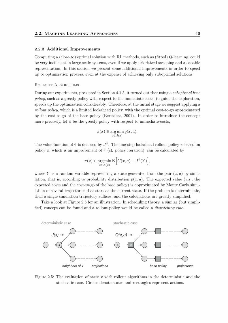
2.2. Machine Learning Approaches 40
2.2.3 Additional Improvements
Computing a (close-to) optimal solution with RL methods, such as (fitted) Q-learning, couldbe very inefficient in large-scale systems, even if we apply prioritized sweeping and a capablerepresentation. In this section we present some additional improvements in order to speedup to optimization process, even at the expense of achieving only suboptimal solutions.
Rollout Algorithms
During our experiments, presented in Section 4.1.5, it turned out that using a suboptimal base
policy, such as a greedy policy with respect to the immediate costs, to guide the exploration,speeds up the optimization considerably. Therefore, at the initial stage we suggest applying arollout policy, which is a limited lookahead policy, with the optimal cost-to-go approximatedby the cost-to-go of the base policy (Bertsekas, 2001). In order to introduce the conceptmore precisely, let π be the greedy policy with respect to immediate-costs,
π(x) ∈ arg mina∈A(x)
g(x, a).
The value function of π is denoted by J π. The one-step lookahead rollout policy π based onpolicy π, which is an improvement of π (cf. policy iteration), can be calculated by
π(x) ∈ arg mina∈A(x)
E
[G(x, a) + J π(Y )
],
where Y is a random variable representing a state generated from the pair (x, a) by simu-lation, that is, according to probability distribution p(x, a). The expected value (viz., theexpected costs and the cost-to-go of the base policy) is approximated by Monte Carlo simu-lation of several trajectories that start at the current state. If the problem is deterministic,then a single simulation trajectory suffices, and the calculations are greatly simplified.
Take a look at Figure 2.5 for an illustration. In scheduling theory, a similar (but simpli-fied) concept can be found and a rollout policy would be called a dispatching rule.
Figure 2.5: The evaluation of state x with rollout algorithms in the deterministic and thestochastic case. Circles denote states and rectangles represent actions.

2.2. Machine Learning Approaches 41
The two main issues why we suggest the application of rollout algorithms are
1. We need several initial samples before the first application of approximation techniquesand these first samples can be generated by simulations guided by a rollout policy.
2. General reinforcement learning methods perform quite poorly in practice without anyinitial guidance. However, the learning algorithm can start improving the rolloutpolicy π, especially, in case we apply (fitted) Q-learning, it can learn directly from thetrajectories generated by a rollout policy, since it is an off-policy learning method.
Action Space Decomposition
In large-scale problems the set of available actions in a state may be very large, which canslow down the system significantly. In the current formulation of the RAP the number ofavailable actions in a state is O(|T | |R|). Though, even in real world situations |R| is, usually,not very large, but T could contain thousands of tasks. Here, we suggest decomposing theaction space as shown in Figure 2.6. First, the system selects a task, only, and it moves to anew state where this task is fixed and an executing resource should be selected. In this casethe state description can be extended by a new variable τ ∈ T ∪ ∅, where ∅ denotes thecase when no task has been selected yet. In every other case the system should select anexecuting resource for the selected task. Consequently, the new action space is A = A1∪A2,where A1 = av | v ∈ T ∪aω and A2 = ar | r ∈ R. As a result, we radically decreasedthe number of available actions, however, the number of possible states was increased, aswell. Nevertheless, our numerical experiments showed that it was a reasonable trade-off.
Figure 2.6: Action selection before (up) and after (down) action space decomposition.

2.2. Machine Learning Approaches 42
Clustering the Tasks
The idea of divide-and-conquer is widely used in artificial intelligence and recently it hasappeared in the theory of dealing with large-scale MDPs. Partitioning a problem intoseveral smaller subproblems is also often applied to decrease computational complexity incombinatorial optimization problems, for example, in scheduling theory.
We propose a simple and still efficient partitioning method for a practically very im-portant class of performance measures. In real world situations the tasks very often haverelease dates and due dates, and the performance measure, e.g., total lateness and numberof tardy tasks, depends on meeting the deadlines. Note that these measures are regular.We denote the (possibly randomized) functions defining the release and due dates of thetasks by A : T → N and B : T → N, respectively. In this section we restrict ourselves toperformance measures that are regular and depend on due dates. In order to cluster thetasks, we need the definition of weighted expected slack time which is given as follows
Sw(v) =∑
s∈Γ(v)
w(s) E
[B(v) −A(v) −D(s, v)
],
where Γ(v) = s ∈ S | 〈s, v〉 ∈ dom(D) denotes the set of resource states in which task vcan be processed, and w(s) are weights corresponding, for example, to the likelihood thatresource state s appears during execution, or they can be simply w(s) = 1/ |Γ(v)|.
Figure 2.7: Clustering the tasks according to their slack times and precedence constraints.
In order to increase computational speed, we suggest clustering the tasks in T into suc-cessive disjoint subsets T1, . . . , Tk according to the precedence constraints and the expectedslack times; take a look at Figure 2.7 for an illustration. The basic idea behind our ap-proach is that we should handle the most constrained tasks first. Therefore, ideally, if Ti
and Tj are two clusters and i < j, then tasks in Ti had expected slack times smaller thantasks in Tj . However, in most of the cases clustering is not so simple, since the precedenceconstraints must also be taken into account and this clustering criterion has the priority.Thus, if 〈u, v〉 ∈ C, u ∈ Ti and v ∈ Tj , i ≤ j must hold. During learning, first, tasks in T1
are allocated to resources, only. After some episodes, we fix the allocation policy concerningtasks in T1 and we start sampling to achieve a good policy for tasks in T2, and so on.

2.2. Machine Learning Approaches 43
Naturally, clustering the tasks is a two-edged weapon, making too small clusters mayseriously decrease the performance of the best achievable policy, making too large clustersmay considerably slow down the system. This technique, however, has several advantages,e.g., (1) it effectively decreases the search space; (2) further reduces the number of availableactions in the states; and, additionally (3) speeds up the learning, since the sample trajecto-ries become smaller (only a small part of the tasks is allocated in a trial and, consequently,the variance of the total costs is decreased). The effects of clustering relative to the size ofthe clusters were analyzed experimentally and are presented in Section 4.1.5.
2.2.4 Distributed Systems
In this section we further improve the previously given solution by distributing the compu-tation of a good control policy among several processor. Before we present our distributedapproach, first, we give an overview on a few widespread distributed optimization techniquesand compare some of their properties, such as the guarantees of finding an optimal (or anear optimal) solution and their robustness against disturbances, such as breakdowns.
In the past decades considerable amount of research was done to enhance decision-making, such as resource allocation, and several new paradigms appeared to distributedoptimization. Distributed decision-making is often favorable (Perkins et al., 1994), not onlybecause it can speed up the computation considerably, but also because it can result in morerobust and flexible solutions. For example, a multi-agent based point of view combined witha heterarchical architecture can show up several advantages (Baker, 1998), such as self-configuration, scalability, fault tolerance, massive parallelism, reduced complexity, increasedflexibility, reduced cost and, last but not least, emergent behavior (Ueda et al., 2001).
Agent Based Approaches
Multi-agent systems (MASs) constitute a popular approach to distributed computation inartificial intelligence. A MAS is a special distributed system with localized decision-makingand, usually, localized storage. An agent is basically a self-directed entity with its own valuesystem and a means to communicate with other such objects (Baker, 1998).
Multi-agent based or holonic manufacturing with adaptive agents received a great dealof recent attention (Baker, 1998; Monostori et al., 2006). They became a promising tool formanaging complexity in manufacturing. A MAS approach to production control is usefulfor manufacturers who often need to change the configuration of their factories by adding orremoving machines, workers, product lines, manufacturers who cannot predict the possiblemanufacturing scenarios according to which they will need to work in the future.
A complex adaptive system (CAS) can be considered as a MAS with highly adaptiveagents (Holland, 1992, 1995). Agents may represent any entity with self-orientation, such ascells, species, individuals, firms or nations. Environmental conditions are changing, due tothe agents’ interactions as they compete and cooperate for the same resources or for achievinga given goal. This, in turn, changes the behavior of the agents themselves. The mostremarkable phenomenon exhibited by a CAS is the emergence of highly structured collective

2.2. Machine Learning Approaches 44
behavior over time from the interactions of simple subsystems. The typical characteristics ofa CAS include dynamics involving interrelated spatial and temporal effects, correlations overlong length- and time-scales, strongly coupled degrees of freedom and non-interchangeablesystem elements, to name only the most important ones. Adaptive agents become importanttools for managing complexity and optimizing diverse types of production control systems(Monostori, 2003; Monostori et al., 2004; Monostori and Csáji, 2006; Schuh et al., 2008).
PROSA (Van Brussel et al., 1998) is a standard MAS based architecture for manufac-turing systems. The general idea underlying this approach is to consider both the resources(e.g., machines) and the jobs (interconnected tasks) as active entities. The basic architectureof the PROSA approach consists of three types of agents: order agents (internal logistics),product agents (process plans), and resource agents (resource handling). Resource agentscorrespond to physical parts (production resources in the system, such as factories, shops,machines, furnaces, conveyors, pipelines, material storages, personnel, etc.), and contain aninformation processing part that controls the resource. Product agents hold the process andproduct knowledge to assure the correct making of the product. They act like informationservers to other agents. Order agents represent a task or a job (an ordered set of tasks) inthe manufacturing system. They are responsible for performing the assigned work correctly,effectively and on time. Though, the PROSA architecture is a production control approach,it is only a framework, it does not offer any direct resource allocation solutions. It is only apossible starting point for designing multi-agent based manufacturing systems.
A lot of distributed optimization techniques were inspired by various biological systems(Kennedy and Eberhart, 1995), such as bird flocks, wolf packs, fish schools, termite hills orant-colonies. These approaches can show up strongly robust and parallel behavior. The ant-
colony optimization algorithm (Moyson and Manderick, 1988) is, in general, a distributedand randomized algorithm to solve shortest path problems in graphs. RAPs can be formu-lated as special stochastic shortest path problems, as well, as we saw in Section 2.1.3.
The PROSA architecture can also be extended by ant-colony type optimization methods(Hadeli et al., 2004). In this case a new type of agent is introduced, called ant. Agents of thistype are mobile and they gather and distribute information in the manufacturing system.The main assumption is that the agents are much faster than the ironware that they control,and that makes the system capable to forecast. Agents are faster and, therefore, can emulatethe behavior of the system several times before the actual decision is taken. The resourceallocation in this system is made by local decisions. Each order agent sends ants (mobile-agents), which are moving downstream in a virtual manner. They gather information aboutthe possible schedules from the resource agents and then they return to the order agent withthe information. The order agent chooses a schedule and then it sends ants to book theneeded resources. After that the order agent regularly sends booking ants to re-book thepreviously found best schedule, because if the booking is not refreshed then it evaporates
after a while (like the pheromone in the analogy of food-foraging ants). From time to timethe order agent sends ants to survey the possible new (and better) schedules. If they finda better solution, the order agent sends ants to book the resources that are needed for thenew schedule and the old booking information will simply evaporate, eventually.

2.2. Machine Learning Approaches 45
Swarm optimization methods are very robust, they can naturally adapt to disturbancesand environmental changes, since the ants continuously explore the current situation and theobsolete data simply evaporates if not refreshed regularly. However, these techniques oftenhave the disadvantage that finding an optimal or even a relatively good solution cannot beeasily guaranteed, theoretically. The ant-colony based extension of PROSA, for example,faces almost exclusively the routing problem in resource allocation and it mostly ignoressequencing problems, namely, it does not concern with the efficient ordering of the tasks.
There are multi-agent systems which use some kinds of negotiation or market-basedmechanism (Márkus et al., 1996). In this case, the tasks or the jobs are associated with orderagents, while the resources are controlled by resource agents, like in the case of PROSA.
Market-based resource allocation is a recursive, iterative process with announce-bid-award cycles. During resource allocation the tasks are announced to the agents that controlthe resources, and they can bid for the available works. The jobs or tasks are, usually,announced one-by-one, which can lead to myopic behavior and, therefore, guaranteeing anoptimal or even an approximately good solution is often very hard. Regarding adaptivebehavior, market-based resource allocation is often less robust than swarm optimizationmethods, such as ant-colony optimization, however, their performance is usually better.
Parallel Optimization
It is known (Modi et al., 2001) that resource allocation problems (at least their deterministicvariants) can be often formulated as constraint satisfaction (CS) problems. In this case, theyaim at solving a multi-dimensional, constraint optimization problem, defined as
optimize f(x1, x2, . . . , xn),
subject to gj(x1, x2, . . . , xn) ≤ cj ,
where xi ∈ Xi, i ∈ 1, . . . , n and j ∈ 1, . . . ,m. Functions f and gj are real-valued andcj ∈ R, as well. Moreover, most RAPs, for example, resource constrained project scheduling,can be formulated as a linear programming (LP) problem, which can be written as follows
optimize 〈c, x〉 ,
subject to Ax ≤ b,
where A ∈ Rn×m, c ∈ Rn, b ∈ Rm and 〈·, ·〉 denotes inner product. Then, distributedvariants of constrained optimization approaches can be applied to compute a solution. Inthis case, a close-to-optimal solution is often guaranteed, however, the computation time isusually large. The main problems with these approaches are that they cannot easily takeuncertainties into account and, moreover, they are not robust against disturbances.
The idea of divide-and-conquer is often applied to decrease computational complexitywhen dealing with combinatorial optimization problems. The main idea behind this ap-proach is to decompose the problem and solve the resulted sub-problems independently. Inmost cases calculating the sub-solutions can be done in a distributed way (Wu et al., 2005).
These approaches can be effectively applied in many cases, however, defining a decom-position which guarantees both efficient computational speedup together with the property

2.2. Machine Learning Approaches 46
that combining the optimal solutions of the sub-problems results in a global optimal solutionis very demanding. Therefore, when we apply decomposition, we usually have to give-upoptimality and satisfy with fast but sometimes far-from-optimal solutions. Moreover, it ishard to make these systems robust against disturbances. Tracking environmental changescan be often accomplished by the complete recalculation of the whole solution, only.
Distributed Sampling
Finally, we argue that the approach presented in Section 2.2 can be easily and efficientlydistributed among several processors with distributed sampling. We will consider extensionsof the algorithm using both shared memory and distributed memory architectures. Take alook at Figure 2.8 for an illustration of these architectures. We suppose that we have kprocessors, and let us denote the set of all processors by P = p1, p2, . . . , pk.
Figure 2.8: Shared (a) and distributed (b) memory access.
In case we have a parallel system with a shared memory architecture, e.g., UMA (uniformmemory access), then it is straightforward to parallelize the computation of a control policy.Namely, each processor p ∈ P can sample the search space independently, while by usingthe same, shared value function. The (joint) control policy can be calculated using thiscommon, global value function, e.g., the greedy policy w.r.t. this function can be applied.
Parallelizing the solution by using an architecture with distributed memory is more chal-lenging. Probably the simplest way to parallelize our approach to several processors withdistributed memory is to let the processors search independently by letting them work-ing with their own, local value functions. After a given time or number of iterations, wemay treat the best achieved solution as the joint policy. More precisely, if we denote theaggregated initial state by x0, then the joint control policy π can be defined as follows
π ∈ arg minπp (p∈P)
Jπp(x0) or π ∈ arg minπp (p∈P)
mina∈A(x0)
Qπp(x0, a),
where Jπp and Qπp are (approximate) state- and action-value functions calculated by proces-sor p ∈ P. Control policy πp is the solution of processor p after a given number of iterations.During our numerical experiments we usually applied 10 000 iterations per processor.
Naturally, there could be many (more sophisticated) ways to parallelize the computationusing several processors with distributed memory. From time to time, e.g., the processorscould exchange some of their best episodes (trajectories with the lowest costs) and learn from
2.2. Machine Learning Approaches 47
the experiments of the others. In this way, they could help improving the value functionsof each other. Our numerical experiments, presented in Section 4.1.3, showed that evenin the simplest case, distributing the calculation speeds up the optimization considerably.Moreover, in case of applying a shared memory architecture, the speedup was almost linear.
As parallel computing represents a very promising way do deal with large-scale sys-tems, their further theoretical and experimental investigation would be very important. Forexample, by harmonizing the exploration of the processors, the speedup could be improved.
Chapter 3
Varying Environments
In Chapter 2 we investigated stochastic RAPs in which some of the components, e.g., theexecuting times, were uncertain. We took the approach to associate the uncertain parameterswith random variables. So far, only the stationary case was studied, however, many problemsthat appear in practise come from the sudden changes of the environment. In this chapterwe analyze how MDP based approaches could work in these circumstances.
The dynamics of stochastic RAPs presented in Chapter 2 can be modeled as MDPs,but what happens when the model was wrong, e.g., if the real transition-probabilities weredifferent, or the dynamics had changed meanwhile? Naturally, the changing of the dynamicscan also be modeled as a (higher level) MDP, however, in this way the problem could veryeasily become practically intractable. In “real word” problems computing an optimal oreven a relatively good policy is extremely time-consuming and the needed computationgrows rapidly with the number of states. Including environmental changes in the model isvery likely to lead to problems which do not have any practically efficient solution method.
In what follows, we argue that if the model was “close” to the environment, then theperformance of a control policy in the model would also be “close” to the performance of thesame policy applied in the real environment and, moreover, “slight” changes in the environ-ment result only in “slight” changes in the value functions. More precisely, we show thatthe value function of a (stationary, Markovian, randomized) control policy in a discountedMDP Lipschitz continuously depends on the immediate-cost and the transition-probability
functions. We also present value function bounds for the case of changes in the discount
factor and demonstrate through an example that this dependence is not Lipschitz contin-uous. Even though optimal policies might also change if the environment has changed, wewill show that these results can be extended to optimal value functions, as well.
As a consequence, it is not unconditionally important to include small dynamics changesin the model. If the dynamics have changed, then the old and obsolete cost-to-go values canbe effectively used as starting points for adapting, since they will not be very far from thechanged value function of the new environment, if the change was not radical. Therefore,for slowly varying systems, we can safely avoid modeling the changes of the dynamics if weuse a method that iteratively approximates the optimal value function. This approach isalso supported by the results of our numerical experiments, presented in Chapter 4.
48
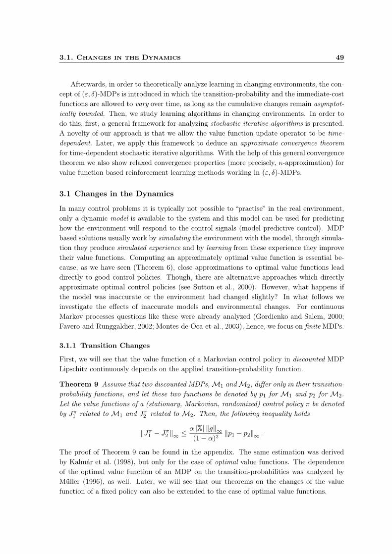
3.1. Changes in the Dynamics 49
Afterwards, in order to theoretically analyze learning in changing environments, the con-cept of (ε, δ)-MDPs is introduced in which the transition-probability and the immediate-costfunctions are allowed to vary over time, as long as the cumulative changes remain asymptot-
ically bounded. Then, we study learning algorithms in changing environments. In order todo this, first, a general framework for analyzing stochastic iterative algorithms is presented.A novelty of our approach is that we allow the value function update operator to be time-
dependent. Later, we apply this framework to deduce an approximate convergence theorem
for time-dependent stochastic iterative algorithms. With the help of this general convergencetheorem we also show relaxed convergence properties (more precisely, κ-approximation) forvalue function based reinforcement learning methods working in (ε, δ)-MDPs.
3.1 Changes in the Dynamics
In many control problems it is typically not possible to “practise” in the real environment,only a dynamic model is available to the system and this model can be used for predictinghow the environment will respond to the control signals (model predictive control). MDPbased solutions usually work by simulating the environment with the model, through simula-tion they produce simulated experience and by learning from these experience they improvetheir value functions. Computing an approximately optimal value function is essential be-cause, as we have seen (Theorem 6), close approximations to optimal value functions leaddirectly to good control policies. Though, there are alternative approaches which directlyapproximate optimal control policies (see Sutton et al., 2000). However, what happens ifthe model was inaccurate or the environment had changed slightly? In what follows weinvestigate the effects of inaccurate models and environmental changes. For continuousMarkov processes questions like these were already analyzed (Gordienko and Salem, 2000;Favero and Runggaldier, 2002; Montes de Oca et al., 2003), hence, we focus on finite MDPs.
3.1.1 Transition Changes
First, we will see that the value function of a Markovian control policy in discounted MDPLipschitz continuously depends on the applied transition-probability function.
Theorem 9 Assume that two discounted MDPs, M1 and M2, differ only in their transition-
probability functions, and let these two functions be denoted by p1 for M1 and p2 for M2.
Let the value functions of a (stationary, Markovian, randomized) control policy π be denoted
by Jπ1 related to M1 and Jπ
2 related to M2. Then, the following inequality holds
‖Jπ1 − Jπ
2 ‖∞ ≤α |X| ‖g‖∞(1 − α)2
‖p1 − p2‖∞ .
The proof of Theorem 9 can be found in the appendix. The same estimation was derivedby Kalmár et al. (1998), but only for the case of optimal value functions. The dependenceof the optimal value function of an MDP on the transition-probabilities was analyzed byMüller (1996), as well. Later, we will see that our theorems on the changes of the valuefunction of a fixed policy can also be extended to the case of optimal value functions.
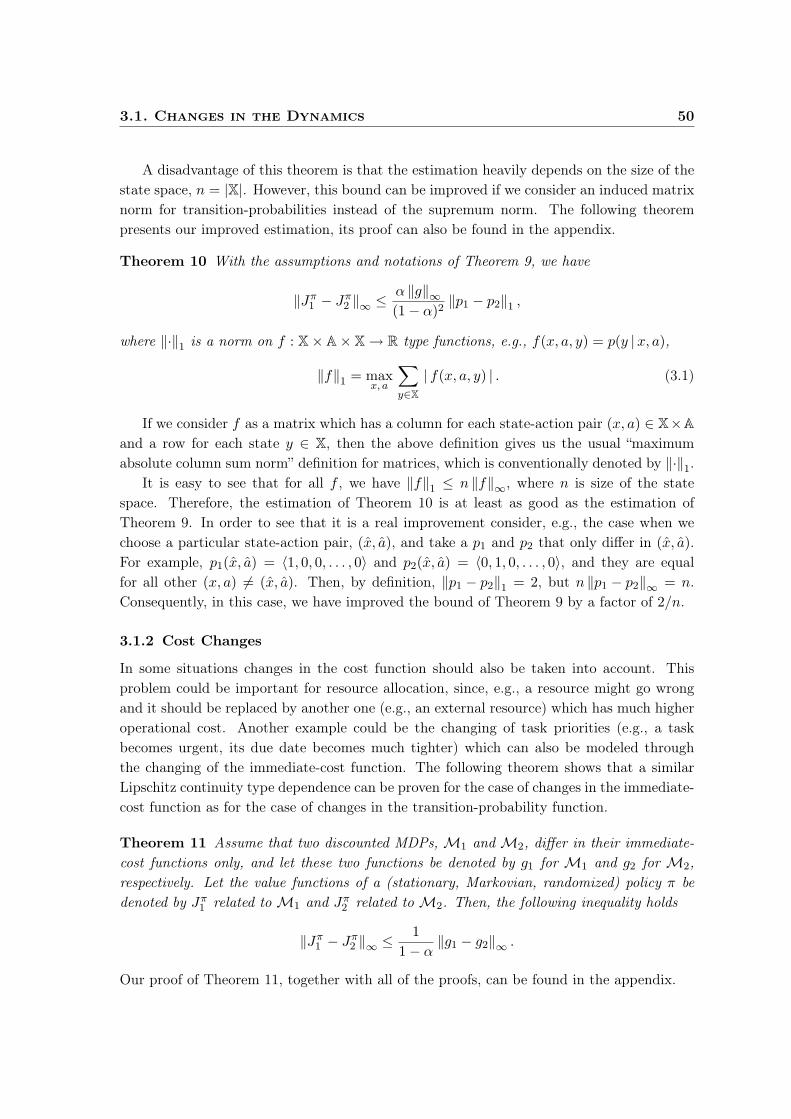
3.1. Changes in the Dynamics 50
A disadvantage of this theorem is that the estimation heavily depends on the size of thestate space, n = |X|. However, this bound can be improved if we consider an induced matrixnorm for transition-probabilities instead of the supremum norm. The following theorempresents our improved estimation, its proof can also be found in the appendix.
Theorem 10 With the assumptions and notations of Theorem 9, we have
‖Jπ1 − Jπ
2 ‖∞ ≤α ‖g‖∞(1 − α)2
‖p1 − p2‖1 ,
where ‖·‖1 is a norm on f : X × A × X → R type functions, e.g., f(x, a, y) = p(y |x, a),
‖f‖1 = maxx, a
∑
y∈X
| f(x, a, y) | . (3.1)
If we consider f as a matrix which has a column for each state-action pair (x, a) ∈ X×A
and a row for each state y ∈ X, then the above definition gives us the usual “maximumabsolute column sum norm” definition for matrices, which is conventionally denoted by ‖·‖1.
It is easy to see that for all f , we have ‖f‖1 ≤ n ‖f‖∞, where n is size of the statespace. Therefore, the estimation of Theorem 10 is at least as good as the estimation ofTheorem 9. In order to see that it is a real improvement consider, e.g., the case when wechoose a particular state-action pair, (x, a), and take a p1 and p2 that only differ in (x, a).For example, p1(x, a) = 〈1, 0, 0, . . . , 0〉 and p2(x, a) = 〈0, 1, 0, . . . , 0〉, and they are equalfor all other (x, a) 6= (x, a). Then, by definition, ‖p1 − p2‖1 = 2, but n ‖p1 − p2‖∞ = n.Consequently, in this case, we have improved the bound of Theorem 9 by a factor of 2/n.
3.1.2 Cost Changes
In some situations changes in the cost function should also be taken into account. Thisproblem could be important for resource allocation, since, e.g., a resource might go wrongand it should be replaced by another one (e.g., an external resource) which has much higheroperational cost. Another example could be the changing of task priorities (e.g., a taskbecomes urgent, its due date becomes much tighter) which can also be modeled throughthe changing of the immediate-cost function. The following theorem shows that a similarLipschitz continuity type dependence can be proven for the case of changes in the immediate-cost function as for the case of changes in the transition-probability function.
Theorem 11 Assume that two discounted MDPs, M1 and M2, differ in their immediate-
cost functions only, and let these two functions be denoted by g1 for M1 and g2 for M2,
respectively. Let the value functions of a (stationary, Markovian, randomized) policy π be
denoted by Jπ1 related to M1 and Jπ
2 related to M2. Then, the following inequality holds
‖Jπ1 − Jπ
2 ‖∞ ≤1
1 − α‖g1 − g2‖∞ .
Our proof of Theorem 11, together with all of the proofs, can be found in the appendix.
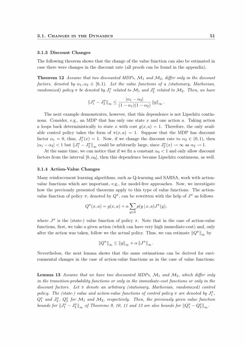
3.1. Changes in the Dynamics 51
3.1.3 Discount Changes
The following theorem shows that the change of the value function can also be estimated incase there were changes in the discount rate (all proofs can be found in the appendix).
Theorem 12 Assume that two discounted MDPs, M1 and M2, differ only in the discount
factors, denoted by α1, α2 ∈ [0, 1). Let the value functions of a (stationary, Markovian,
randomized) policy π be denoted by Jπ1 related to M1 and Jπ
2 related to M2. Then, we have
‖Jπ1 − Jπ
2 ‖∞ ≤|α1 − α2|
(1 − α1)(1 − α2)‖g‖∞ .
The next example demonstrates, however, that this dependence is not Lipschitz contin-uous. Consider, e.g., an MDP that has only one state x and one action a. Taking actiona loops back deterministically to state x with cost g(x, a) = 1. Therefore, the only avail-able control policy takes the form of π(x, a) = 1. Suppose that the MDP has discountfactor α1 = 0, thus, Jπ
1 (x) = 1. Now, if we change the discount rate to α2 ∈ (0, 1), then|α1 − α2| < 1 but ‖Jπ
1 − Jπ2 ‖∞ could be arbitrarily large, since Jπ
2 (x) → ∞ as α2 → 1.At the same time, we can notice that if we fix a constant α0 < 1 and only allow discount
factors from the interval [0, α0], then this dependence became Lipschitz continuous, as well.
3.1.4 Action-Value Changes
Many reinforcement learning algorithms, such as Q-learning and SARSA, work with action-value functions which are important, e.g., for model-free approaches. Now, we investigatehow the previously presented theorems apply to this type of value functions. The action-value function of policy π, denoted by Qπ, can be rewritten with the help of Jπ as follows
Qπ(x, a) = g(x, a) + α∑
y∈X
p(y |x, a)Jπ(y),
where Jπ is the (state-) value function of policy π. Note that in the case of action-valuefunctions, first, we take a given action (which can have very high immediate-cost) and, onlyafter the action was taken, follow we the actual policy. Thus, we can estimate ‖Qπ‖∞ by
‖Qπ‖∞ ≤ ‖g‖∞ + α ‖Jπ‖∞ .
Nevertheless, the next lemma shows that the same estimations can be derived for envi-ronmental changes in the case of action-value functions as in the case of value functions.
Lemma 13 Assume that we have two discounted MDPs, M1 and M2, which differ only
in the transition-probability functions or only in the immediate-cost functions or only in the
discount factors. Let π denote an arbitrary (stationary, Markovian, randomized) control
policy. The (state-) value and action-value functions of control policy π are denoted by Jπ1 ,
Qπ1 and Jπ
2 , Qπ2 for M1 and M2, respectively. Then, the previously given value function
bounds for ‖Jπ1 − Jπ
2 ‖∞ of Theorems 9, 10, 11 and 12 are also bounds for ‖Qπ1 −Qπ
2‖∞.
3.1. Changes in the Dynamics 52
3.1.5 Optimal Cost-to-Go Changes
Another interesting question is the effects of environmental changes on the optimal valuefunction. Theorems 9, 10, 11 and 12 cannot be directly applied to deduce estimations forthe case of optimal value functions, since they presuppose that the policy is fixed, however,optimal policies might also change if the environment had changed. Nevertheless, with thehelp of the following lemma, the case of optimal value functions becomes a consequence ofthe previous theorems. The proof of Lemma 14 can be found in the appendix, as well.
Lemma 14 For all f1, f2 : X → R bounded functions such that minx f1(x) ≤ minx f2(x)
and x = arg minx f1(x), we have the inequality |minx f1(x) − minx f2(x)| ≤ |f1(x) − f2(x)|.
Assume that we have two discounted MDPs, M1 and M2, which may differ in theirtransition-probability functions, immediate-cost functions and discount factors. In order todeduce bounds for the distance of their optimal value functions, first, let us introduce anauxiliary (stationary, Markovian) deterministic control policy, defined as follows
π(x) =
π∗1(x) if J∗1 (x) ≤ J∗
2 (x),
π∗2(x) if J∗2 (x) < J∗
1 (x),
where π∗i denotes an optimal control policy in Mi and J∗i is the optimal value function of
Mi, i ∈ 1, 2. Policy π∗i can be, e.g., a greedy policy w.r.t. J∗i (cf. Theorem 6). Then, by
using the Bellman equation in the first step and Lemma 14 in the second, we have
∀x ∈ X : |J∗1 (x) − J∗
2 (x)| =
=
∣∣∣∣∣∣min
a∈A(x)
[g1(x, a) + α1
∑
y∈X
p1(y | x, a)J∗1 (y)
]−
− mina∈A(x)
[g2(x, a) + α2
∑
y∈X
p2(y | x, a)J∗2 (y)
]∣∣∣∣∣∣≤
≤
∣∣∣∣∣∣g1(x, π(x)) + α1
∑
y∈X
p1(y | x, π(x))J∗1 (y)−
− g2(x, π(x)) − α2
∑
y∈X
p2(y | x, π(x))J∗2 (y)
∣∣∣∣∣∣=
=∣∣∣J π
1 (x) − J π2 (x)
∣∣∣ .
Therefore, with the help of Lemma 14, we reduced the case of changes in the optimal valuefunction to the case of changes in the value function of a fixed policy, namely π. This resultis precisely stated in Corollary 15. It allows us to extend Theorems 9, 10, 11 and 12 to thecase of optimal value functions, as well, which consequence is summarized by Corollary 16.
3.1. Changes in the Dynamics 53
Corollary 15 Assume that we have two discounted MDPs, M1 and M2, which may differ
in their transition functions, cost functions and discount factors. Let us denote the optimal
value functions of M1 and M2 by J∗1 and J∗
2 , respectively. Then, there exists a (stationary,
Markovian, deterministic) control policy π such that ‖J∗1 − J∗
2‖∞ ≤ ‖Jπ1 − Jπ
2 ‖∞.
Since deterministic control policies are special cases of randomized ones, we also have:
Corollary 16 Assume that we have two discounted MDPs which differ only in the transition-
probability functions or only in the immediate-cost functions or only in the discount factors.
Let the corresponding optimal value functions be denoted by J∗1 and J∗
2 , respectively. Then,
the bounds for ‖Jπ1 − Jπ
2 ‖∞ of Theorems 9, 10, 11 and 12 are also bounds for ‖J∗1 − J∗
2‖∞.
It is straightforward to see that these results can be extended to optimal action-value
functions, as well. One should apply the same “trick” as before and introduce an auxiliarycontrol policy by which the difference of the optimal action-value functions can be estimatedfrom above. In fact, the same control policy, namely π, can be applied to achieve this.
Corollary 17 Assume that we have two discounted MDPs which differ only in the transition-
probability functions or only in the immediate-cost functions or only in the discount factors.
The corresponding optimal action-value functions are denoted by Q∗1 and Q∗
2, respectively.
Then, the value function bounds for ‖Jπ1 − Jπ
2 ‖∞ are also bounds for ‖Q∗1 −Q∗
2‖∞.
3.1.6 Further Remarks
In the previous parts of the section we saw that value functions of discounted MDPs de-pend smoothly on the transition-probability function, the immediate-cost function and thediscount rate. This dependence is of Lipschitz type in the first two cases and non-Lipschitzfor discount rates. Later, we will see that changes in the discount factor can be traced backto changes in the immediate-cost function (Lemma 24), therefore, it is sufficient to considertransition and cost changes. The following corollary summarizes some of the results.
Corollary 18 Assume that two discounted MDPs, E and M, differ only in their transition-
probability functions and their immediate-cost functions. The corresponding transition and
cost functions are denoted by pE , pM and gE , gM. Let the value functions of a (stationary,
Markovian, randomized) control policy π be denoted by JπE and Jπ
M, respectively. Then,
‖JπE − Jπ
M‖∞ ≤‖gE − gM‖∞
1 − α+c α ‖pE − pM‖1
(1 − α)2,
where c = min‖gE‖∞ , ‖gM‖∞ and α ∈ [0, 1) is, as usually, the discount factor.
The proof simply follows from Theorems 10 and 11 and from the triangle inequality. Ifwe treat one of the MDPs in the previous theorems as a system which describes the “real”behavior of the environment and the other MDP as our model relatedly, then these resultsshow that even if the model used is slightly inaccurate or there were changes in the envi-ronment, the optimal value function based on the model cannot be arbitrarily wrong from
3.1. Changes in the Dynamics 54
the viewpoint of the environment. These theorems are of special interest because in “realworld” problems the transitions and the costs are mostly estimated only, e.g., by statisticalmethods from historical data, the exact values are unknown and may even change over time.
Now, we investigate few supplementary results of the presented statements, e.g., someconnections with other results as well as two counterexamples for the undiscounted case.
Average Cost Case
Though, the largest part of the MDP related research studies the expected total discountedcost optimality criterion, in some cases discounting is inappropriate and, therefore, there arealternative optimality approaches, as well. A popular alternative approach is to optimizethe expected average cost (Bertsekas, 2001). In this case the value function is defined as
Jπ(x) = lim supN→∞
1
NE
[N−1∑
t=0
g(Xt, Aπt )
∣∣∣∣ X0 = x
],
where the notations are the same as previously, e.g., as applied in equation (1.1).Regarding the validity of Corollary 16 concerning MDPs with the average cost mini-
mization objective, we can recall the well-known result that, in the case of finite MDPs,discounted cost offers a good approximation to the other optimality criterion. More pre-cisely, it can be shown that there exists a large enough α0 < 1 such that ∀α ∈ (α0, 1)
optimal control policies for the discounted cost problem are also optimal for the averagecost problem (Feinberg and Shwartz, 2002). These policies are called Blackwell optimal.
Simulation Lemma
The results presented in this section have some similarities with the “Simulation Lemma”of Kearns and Singh (2002). They apply that lemma to deduce polynomial time boundsto achieve near-optimal return in MDPs. The Simulation Lemma states that if two MDPsdiffer only in their transition functions and their cost functions and we want to approximate(w.r.t. supremum norm) the value function of a fixed control policy concerning one of theMDPs in the other MDP, then how close should we choose the transition-probabilities andthe immediate-costs to the original MDP relative to the mixing time (in the undiscountedcase) or the horizon time (in the discounted case). Nonetheless, they arrive at a differentkind of bound than we did and, additionally, they only consider the case when the distancesof both the transition and the cost functions are determined by the same parameter.
State and Action Changes
In theory, changes in the state space can be traced back to changes in the control actionspace, because, for example, the deletion of a state can be treated as the deletion of allactions which lead to it, and moreover, adding a new state can be treated as adding somenew actions that lead to a state that was previously unreachable. Additionally, changes inthe control space can be traced back to changes in the cost function or in the transition-probability function. We can treat, e.g., the costs of all controls which are unavailable as
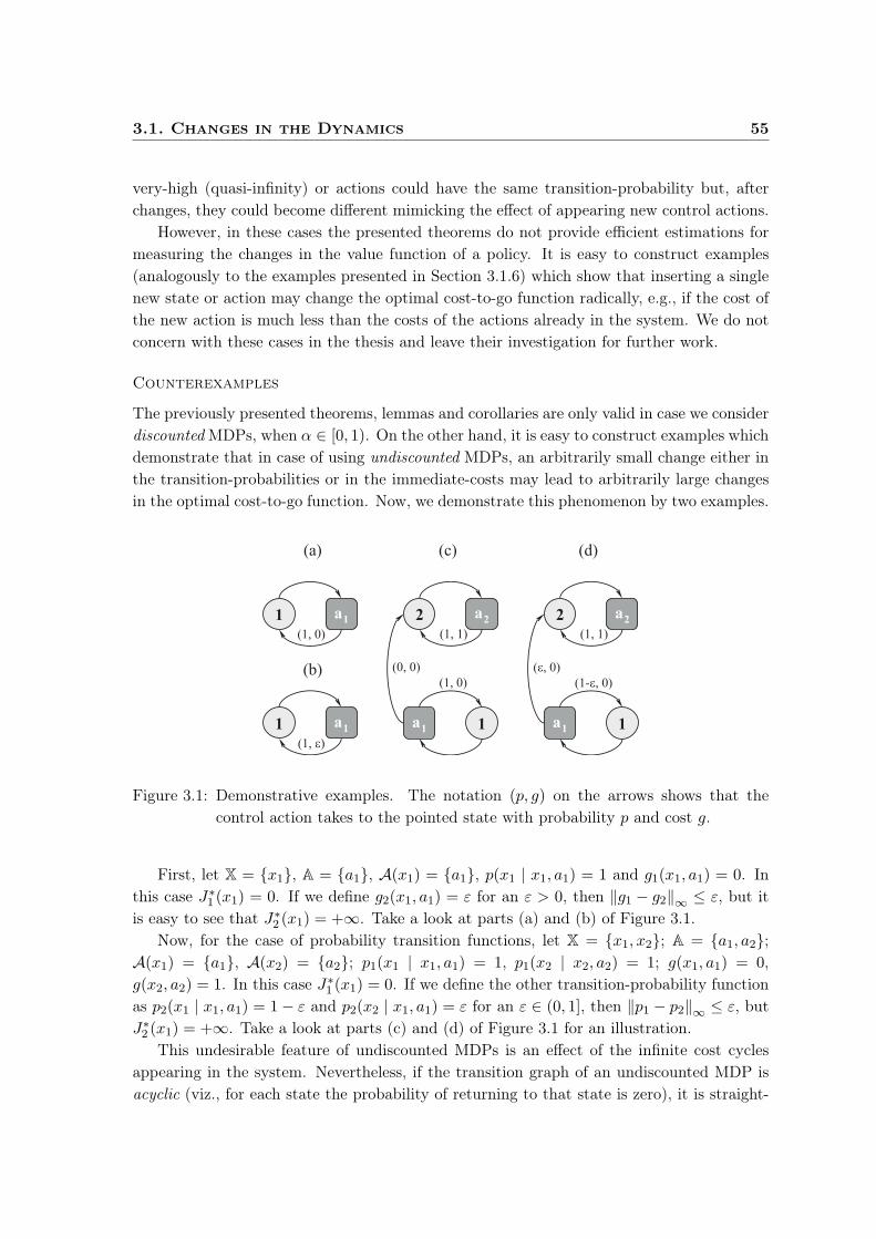
3.1. Changes in the Dynamics 55
very-high (quasi-infinity) or actions could have the same transition-probability but, afterchanges, they could become different mimicking the effect of appearing new control actions.
However, in these cases the presented theorems do not provide efficient estimations formeasuring the changes in the value function of a policy. It is easy to construct examples(analogously to the examples presented in Section 3.1.6) which show that inserting a singlenew state or action may change the optimal cost-to-go function radically, e.g., if the cost ofthe new action is much less than the costs of the actions already in the system. We do notconcern with these cases in the thesis and leave their investigation for further work.
Counterexamples
The previously presented theorems, lemmas and corollaries are only valid in case we considerdiscounted MDPs, when α ∈ [0, 1). On the other hand, it is easy to construct examples whichdemonstrate that in case of using undiscounted MDPs, an arbitrarily small change either inthe transition-probabilities or in the immediate-costs may lead to arbitrarily large changesin the optimal cost-to-go function. Now, we demonstrate this phenomenon by two examples.
Figure 3.1: Demonstrative examples. The notation (p, g) on the arrows shows that thecontrol action takes to the pointed state with probability p and cost g.
First, let X = x1, A = a1, A(x1) = a1, p(x1 | x1, a1) = 1 and g1(x1, a1) = 0. Inthis case J∗
1 (x1) = 0. If we define g2(x1, a1) = ε for an ε > 0, then ‖g1 − g2‖∞ ≤ ε, but itis easy to see that J∗
2 (x1) = +∞. Take a look at parts (a) and (b) of Figure 3.1.Now, for the case of probability transition functions, let X = x1, x2; A = a1, a2;
A(x1) = a1, A(x2) = a2; p1(x1 | x1, a1) = 1, p1(x2 | x2, a2) = 1; g(x1, a1) = 0,g(x2, a2) = 1. In this case J∗
1 (x1) = 0. If we define the other transition-probability functionas p2(x1 | x1, a1) = 1 − ε and p2(x2 | x1, a1) = ε for an ε ∈ (0, 1], then ‖p1 − p2‖∞ ≤ ε, butJ∗
2 (x1) = +∞. Take a look at parts (c) and (d) of Figure 3.1 for an illustration.This undesirable feature of undiscounted MDPs is an effect of the infinite cost cycles
appearing in the system. Nevertheless, if the transition graph of an undiscounted MDP isacyclic (viz., for each state the probability of returning to that state is zero), it is straight-
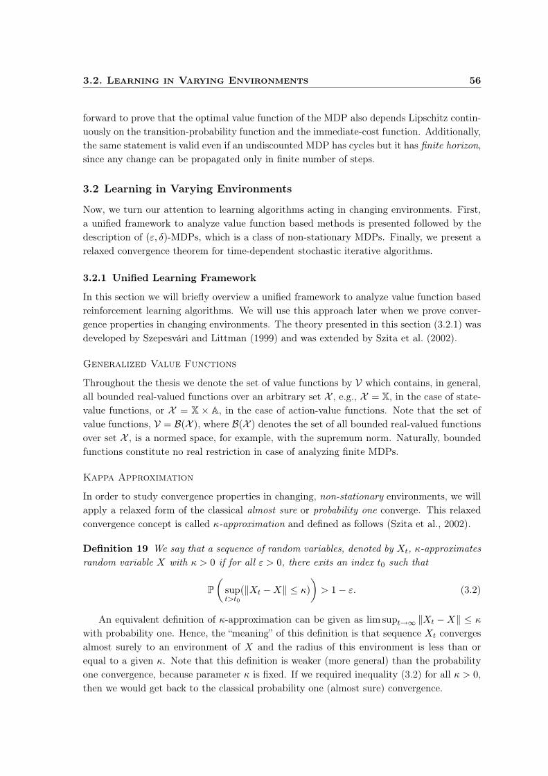
3.2. Learning in Varying Environments 56
forward to prove that the optimal value function of the MDP also depends Lipschitz contin-uously on the transition-probability function and the immediate-cost function. Additionally,the same statement is valid even if an undiscounted MDP has cycles but it has finite horizon,since any change can be propagated only in finite number of steps.
3.2 Learning in Varying Environments
Now, we turn our attention to learning algorithms acting in changing environments. First,a unified framework to analyze value function based methods is presented followed by thedescription of (ε, δ)-MDPs, which is a class of non-stationary MDPs. Finally, we present arelaxed convergence theorem for time-dependent stochastic iterative algorithms.
3.2.1 Unified Learning Framework
In this section we will briefly overview a unified framework to analyze value function basedreinforcement learning algorithms. We will use this approach later when we prove conver-gence properties in changing environments. The theory presented in this section (3.2.1) wasdeveloped by Szepesvári and Littman (1999) and was extended by Szita et al. (2002).
Generalized Value Functions
Throughout the thesis we denote the set of value functions by V which contains, in general,all bounded real-valued functions over an arbitrary set X , e.g., X = X, in the case of state-value functions, or X = X × A, in the case of action-value functions. Note that the set ofvalue functions, V = B(X ), where B(X ) denotes the set of all bounded real-valued functionsover set X , is a normed space, for example, with the supremum norm. Naturally, boundedfunctions constitute no real restriction in case of analyzing finite MDPs.
Kappa Approximation
In order to study convergence properties in changing, non-stationary environments, we willapply a relaxed form of the classical almost sure or probability one converge. This relaxedconvergence concept is called κ-approximation and defined as follows (Szita et al., 2002).
Definition 19 We say that a sequence of random variables, denoted by Xt, κ-approximates
random variable X with κ > 0 if for all ε > 0, there exits an index t0 such that
P
(supt>t0
(‖Xt −X‖ ≤ κ)
)> 1 − ε. (3.2)
An equivalent definition of κ-approximation can be given as lim supt→∞ ‖Xt −X‖ ≤ κ
with probability one. Hence, the “meaning” of this definition is that sequence Xt convergesalmost surely to an environment of X and the radius of this environment is less than orequal to a given κ. Note that this definition is weaker (more general) than the probabilityone convergence, because parameter κ is fixed. If we required inequality (3.2) for all κ > 0,then we would get back to the classical probability one (almost sure) convergence.

3.2. Learning in Varying Environments 57
Generalized Value Iteration
A general form of value iteration type algorithms can be given as follows,
Vt+1 = Ht(Vt, Vt),
where Ht is a random operator on V × V → V (Szepesvári and Littman, 1999). Consider,e.g., the SARSA (State-Action-Reward-State-Action) algorithm which is a model-free policyevaluation method. It aims at finding Qπ for a given policy π and it is defined as
Qt+1(x, a) = (1 − γt(x, a))Qt(x, a) + γt(x, a)(g(x, a) + αQt(Y,B)),
where γt(x, a) denotes the stepsize associated with state x and action a at time t; Y and Bare random variables, Y is generated from the pair (x, a) by simulation, that is, accordingto the distribution p(x, a), and the distribution of B is π(Y ). In this case, Ht is defined as
Ht(Qa, Qb)(x, a) = (1 − γt(x, a))Qa(x, a) + γt(x, a)(g(x, a) + αQb(Y,B)), (3.3)
for all x and a. Therefore, the SARSA algorithm takes the form Qt+1 = Ht(Qt, Qt).
Definition 20 We say that the operator sequence Ht κ-approximates operator H : V → V
at V ∈ V if for any initial V0 ∈ V the sequence Vt+1 = Ht(Vt, V ) κ-approximates HV .
Asymptotic Convergence Bounds
The next theorem (Szita et al., 2002) will be an important tool for proving convergenceresults for value function based RL algorithms working in varying environments.
Theorem 21 Let H be an arbitrary mapping with fixed point V ∗, and let Ht κ-approximate
H at V ∗ over set X . Additionally, assume that there exist random functions 0 ≤ Ft(x) ≤ 1
and 0 ≤ Gt(x) ≤ 1 satisfying the four conditions below with probability one
1. For all V1, V2 ∈ V and for all x ∈ X ,
|Ht(V1, V∗)(x) −Ht(V2, V
∗)(x)| ≤ Gt(x) |V1(x) − V2(x)| .
2. For all V1, V2 ∈ V and for all x ∈ X ,
|Ht(V1, V∗)(x) −Ht(V1, V2)(x)| ≤ Ft(x) ‖V
∗ − V2‖∞ .
3. For all k > 0,∏n
t=k Gt(x) converges to zero uniformly in x as n increases.
4. There exist 0 ≤ ξ < 1 such that for all x ∈ X and sufficiently large t,
Ft(x) ≤ ξ (1 −Gt(x)).
Then, Vt+1 = Ht(Vt, Vt) κ′-approximates V ∗ over X for any V0 ∈ V, where κ′ = 2κ/(1− ξ).

3.2. Learning in Varying Environments 58
Usually, functions Ft and Gt can be interpreted as the ratio of mixing the two argumentsof operator Ht. In the case of the SARSA algorithm, described above by (3.3), X = X × A,Gt(x, a) = (1 − γt(x, a)) and Ft(x, a) = αγt(x, a) would be a suitable choice.
One of the most important aspects of this theorem is that it shows how to reducethe problem of approximating V ∗ with Vt = Ht(Vt, Vt) type operators to the problem ofapproximating it with a V ′
t = Ht(V′t , V
∗) sequence, which is, in many cases, much easier tobe dealt with. This makes, e.g., the convergence of Watkins’ Q-learning a consequence ofthe classical Robbins-Monro theory (Szepesvári and Littman, 1999; Szita et al., 2002).
3.2.2 Varying Markov Decision Processes
Section 3.2 aims at analyzing how learning algorithms can act in environments which maychange over time, namely, in the transition-probability function and the immediate-costfunction. However, without any restrictions, this approach would be too general to establishconvergence results. Therefore, we restrict ourselves to the case when the cumulative changesremain bounded over time. In order to precisely define this concept, the idea of (ε, δ)-MDPsis introduced, which is a generalization of classical MDPs and ε-MDPs.
First, we recall the definition of ε-MDPs (Kalmár et al., 1998; Szita et al., 2002).
Definition 22 A sequence of MDPs (Mt)∞t=1 is called an ε-MDP with ε > 0 if the MDPs
differ only in their transition-probability functions, denoted by pt for Mt, and there exists
an MDP with transition function p, called the base MDP, such that supt ‖p− pt‖ ≤ ε.
Now, we extend the idea described above. The following definition of (ε, δ)-MDPs gen-eralizes the concept of ε-MDPs in two ways. First, we also allow the cost function to changeover time and, additionally, we require the changes to remain bounded by parameters ε andδ only asymptotically, in the limit. A finite number of large deviations is tolerated.
Definition 23 A tuple 〈X,A,A, pt∞t=1, gt
∞t=1, α〉 is an (ε, δ)-MDP with ε, δ ≥ 0, if there
exists an MDP 〈X,A,A, p, g, α〉, called the base MDP (take a look at Figure 3.2), such that
1. lim supt→∞
‖p− pt‖ ≤ ε
2. lim supt→∞
‖g − gt‖ ≤ δ
The optimal value function of the base MDP and of the current MDP at time t (which MDP
has transition function pt and cost function gt) are denoted by J∗ and J∗t , respectively.
In order to keep the analysis as simple as possible, we do not allow the discount rateparameter α to change over time; not only because, e.g., with Theorem 12 at hand, it wouldbe straightforward to extend the results to the case of changing discount factors, but evenmore because, as Lemma 24 demonstrates, the effects of changes in the discount rate can beincorporated into the immediate-cost function, which is allowed to change in (ε, δ)-MDPs.

3.2. Learning in Varying Environments 59
Lemma 24 Assume that two discounted MDPs, M1 and M2, differ only in the discount
factors, denoted by α1 and α2. Let the value function of a (stationary, Markovian, random-
ized) control policy π be denoted by Jπi related to Mi. The optimal value function of Mi is
denoted by J∗i . We will treat both cases simultaneously, thus, let us fix hyper-parameter µ to
either π or ∗. Then, there exists an MDP, denoted by M3, such that it differs only in the
immediate-cost function from M1 and Jµ2 = Jµ
3 . The immediate-cost function of M3 is
g(x, a) = g(x, a) + (α2 − α1)∑
y∈X
p(y |x, a)Jµ2 (y),
where p is the transition-probability function of M1, M2 and M3; g is the immediate-cost
function of M1 and M2; and Jµ2 (y) denotes a value function of M2, where µ ∈ π, ∗.
On the other hand, we can notice that changes in the cost function cannot be tracedback to changes in the transition function. Consider, e.g., an MDP with a constant zero costfunction. Then, no matter what the transition-probabilities are, the optimal value functionremains zero. However, we may achieve non-zero optimal value function values if we changethe immediate-cost function. Therefore, (ε, δ)-MDPs cannot be traced back to ε-MDPs.
Figure 3.2: The transition-probabilities and the costs of an (ε, δ)-MDP may vary arbitrarily,as long as their distances from the base values remain asymptotically bounded.
Now, we briefly investigate the applicability of (ε, δ)-MDPs and a possible motivationbehind them. When we model a “real world” problem as an MDP, then we typically takeonly the major characteristics of the system into account, but there could be many hidden
parameters, as well, which may affect the transition-probabilities and the immediate-costs,however, which are not explicitly included in the model. For example, if we model a pro-duction control system as an MDP (Csáji and Monostori, 2006b), then the workers’ fatigue,mood or the quality of the materials may affect the durations of the tasks, but these char-acteristics are usually not included in the model. Additionally, the values of these hiddenparameters may change over time. In these cases, we could either try to incorporate as manyaspects of the system as possible into the model, which approach would most likely lead tocomputationally intractable results, or we could model the system as an (ε, δ)-MDP instead,which would result in a simplified model and, presumably, in a more tractable system.

3.2. Learning in Varying Environments 60
3.2.3 Stochastic Iterative Algorithms
In this section we present a general relaxed convergence theorem for a large class of stochas-tic iterative algorithms. Later, we will apply this theorem to investigate the convergenceproperties of value function based reinforcement learning methods in (ε, δ)-MDPs.
Many learning and optimization methods can be written in a general form as a stochasticiterative algorithm (Bertsekas and Tsitsiklis, 1996). In general, these algorithms are definedby the iteration rt+1 = (1 − γt)rt + γtst, where the updates are performed on rt, γt is anonnegative stepsize parameter and st is usually a function of rt, for example, st = Htrt.
One of the simplest such algorithm is the Robbins-Monro stochastic approximation algo-
rithm, defined as follows. Let qt be a sequence of independent identically-distributed (i.i.d.)random variables with unknown mean µ and finite variance. Let us define sequence rt withthe iteration rt+1 = (1 − γt)rt + γtqt. Then, sequence rt converges almost surely to µ ifsuitable assumptions on the stepsizes are made, cf. with Assumption 2 of this section.
Another classical example of a stochastic iterative algorithm is the stochastic gradient
descent algorithm which aims at minimizing cost function f and is described by
rt+1 = (1 − γt)rt + γt(rt −∇f(rt) + wt),
where wt is a noise parameter, cf. Assumption 1, and ∇f denotes the gradient of f .
Time-Dependent Update
During Section 3.2.3 we study time-dependent stochastic iterative algorithms of the form
Vt+1(x) = (1 − γt(x))Vt(x) + γt(x)((KtVt)(x) +Wt(x)), (3.4)
where Vt ∈ V, operator Kt : V → V acts on value functions, each γt(x) is a random variablewhich determines the stepsize and Wt(x) is also a random variable, a noise parameter.
Regarding reinforcement learning algorithms, for example, (asynchronous) value itera-tion, Gauss-Seidel methods, Q-learning, SARSA and TD(λ) can be formulated this way.We will show that under suitable conditions these algorithms work in (ε, δ)-MDPs, moreprecisely, κ-approximation to the optimal value function of the base MDP will be proven.
Main Assumptions
Now, in order to provide our relaxed convergence result, we introduce three assumptions onthe noise parameters, the stepsize parameters and the value function operator.
Definition 25 We denote the history of the algorithm until time t by Ft, defined as
Ft = V0, . . . , Vt,W0, . . . ,Wt−1, γ0, . . . , γt .
The sequence F0 ⊆ F1 ⊆ F2 ⊆ ... can be seen as a filtration, viz., as an increasingsequence of σ-fields. The set Ft represents the information available at each time t.
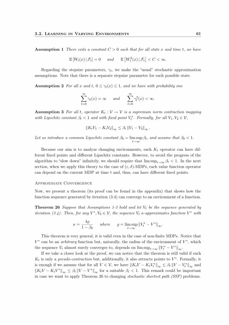
3.2. Learning in Varying Environments 61
Assumption 1 There exits a constant C > 0 such that for all state x and time t, we have
E [Wt(x) | Ft] = 0 and E[W 2
t (x) | Ft
]< C <∞.
Regarding the stepsize parameters, γt, we make the “usual” stochastic approximationassumptions. Note that there is a separate stepsize parameter for each possible state.
Assumption 2 For all x and t, 0 ≤ γt(x) ≤ 1, and we have with probability one
∞∑
t=0
γt(x) = ∞ and∞∑
t=0
γ2t (x) <∞.
Assumption 3 For all t, operator Kt : V → V is a supremum norm contraction mapping
with Lipschitz constant βt < 1 and with fixed point V ∗t . Formally, for all V1, V2 ∈ V,
‖KtV1 −KtV2‖∞ ≤ βt ‖V1 − V2‖∞ .
Let us introduce a common Lipschitz constant β0 = lim supt→∞
βt, and assume that β0 < 1.
Because our aim is to analyze changing environments, each Kt operator can have dif-ferent fixed points and different Lipschitz constants. However, to avoid the progress of thealgorithm to “slow down” infinitely, we should require that lim supt→∞ βt < 1. In the nextsection, when we apply this theory to the case of (ε, δ)-MDPs, each value function operatorcan depend on the current MDP at time t and, thus, can have different fixed points.
Approximate Convergence
Now, we present a theorem (its proof can be found in the appendix) that shows how thefunction sequence generated by iteration (3.4) can converge to an environment of a function.
Theorem 26 Suppose that Assumptions 1-3 hold and let Vt be the sequence generated by
iteration (3.4). Then, for any V ∗, V0 ∈ V, the sequence Vt κ-approximates function V ∗ with
κ =4%
1 − β0where % = lim sup
t→∞‖V ∗
t − V ∗‖∞.
This theorem is very general, it is valid even in the case of non-finite MDPs. Notice thatV ∗ can be an arbitrary function but, naturally, the radius of the environment of V ∗, whichthe sequence Vt almost surely converges to, depends on lim supt→∞ ‖V ∗
t − V ∗‖∞.If we take a closer look at the proof, we can notice that the theorem is still valid if each
Kt is only a pseudo-contraction but, additionally, it also attracts points to V ∗. Formally, itis enough if we assume that for all V ∈ V, we have ‖KtV −KtV
∗t ‖∞ ≤ βt ‖V − V ∗
t ‖∞ and‖KtV −KtV
∗‖∞ ≤ βt ‖V − V ∗‖∞ for a suitable βt < 1. This remark could be importantin case we want to apply Theorem 26 to changing stochastic shortest path (SSP) problems.
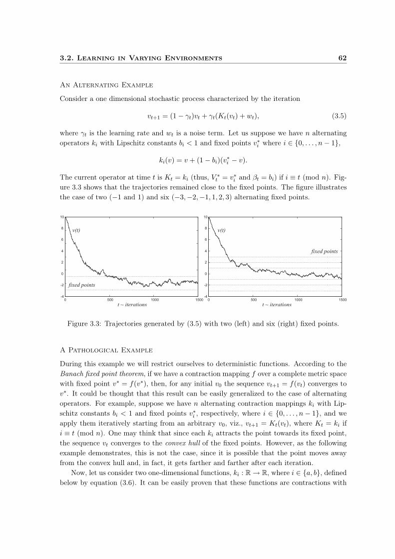
3.2. Learning in Varying Environments 62
An Alternating Example
Consider a one dimensional stochastic process characterized by the iteration
vt+1 = (1 − γt)vt + γt(Kt(vt) + wt), (3.5)
where γt is the learning rate and wt is a noise term. Let us suppose we have n alternatingoperators ki with Lipschitz constants bi < 1 and fixed points v∗i where i ∈ 0, . . . , n− 1,
ki(v) = v + (1 − bi)(v∗i − v).
The current operator at time t is Kt = ki (thus, V ∗t = v∗i and βt = bi) if i ≡ t (mod n). Fig-
ure 3.3 shows that the trajectories remained close to the fixed points. The figure illustratesthe case of two (−1 and 1) and six (−3,−2,−1, 1, 2, 3) alternating fixed points.
0 500 1000 1500-4
-2
0
2
4
6
8
10
t ~ iterations iterationst ~
v(t) v(t)
fixed points
fixed points
-4
-2
0
2
4
6
8
10
0 500 1000 1500
Figure 3.3: Trajectories generated by (3.5) with two (left) and six (right) fixed points.
A Pathological Example
During this example we will restrict ourselves to deterministic functions. According to theBanach fixed point theorem, if we have a contraction mapping f over a complete metric spacewith fixed point v∗ = f(v∗), then, for any initial v0 the sequence vt+1 = f(vt) converges tov∗. It could be thought that this result can be easily generalized to the case of alternatingoperators. For example, suppose we have n alternating contraction mappings ki with Lip-schitz constants bi < 1 and fixed points v∗i , respectively, where i ∈ 0, . . . , n− 1, and weapply them iteratively starting from an arbitrary v0, viz., vt+1 = Kt(vt), where Kt = ki ifi ≡ t (mod n). One may think that since each ki attracts the point towards its fixed point,the sequence vt converges to the convex hull of the fixed points. However, as the followingexample demonstrates, this is not the case, since it is possible that the point moves awayfrom the convex hull and, in fact, it gets farther and farther after each iteration.
Now, let us consider two one-dimensional functions, ki : R → R, where i ∈ a, b, definedbelow by equation (3.6). It can be easily proven that these functions are contractions with
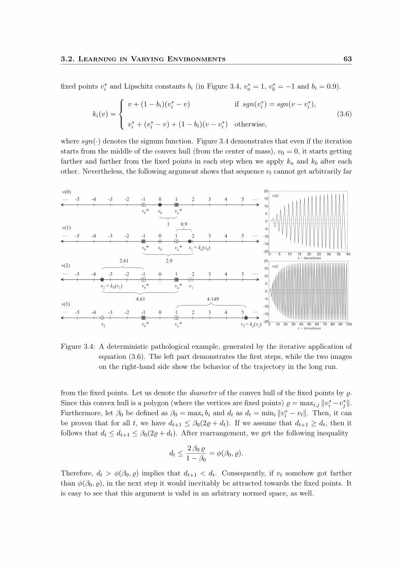
3.2. Learning in Varying Environments 63
fixed points v∗i and Lipschitz constants bi (in Figure 3.4, v∗a = 1, v∗b = −1 and bi = 0.9).
ki(v) =
v + (1 − bi)(v∗i − v) if sgn(v∗i ) = sgn(v − v∗i ),
v∗i + (v∗i − v) + (1 − bi)(v − v∗i ) otherwise,(3.6)
where sgn(·) denotes the signum function. Figure 3.4 demonstrates that even if the iterationstarts from the middle of the convex hull (from the center of mass), v0 = 0, it starts gettingfarther and farther from the fixed points in each step when we apply ka and kb after eachother. Nevertheless, the following argument shows that sequence vt cannot get arbitrarily far
0 1 2 3 4 5 …-1-2-3-4-5…
vb* va*v0
0 1 2 3 4 5-1-2-3-4-5… …
v1 = ka(v0)
0 1 2 3 4 5-1-2-3-4-5… …
v2 = kb(v1)
1
vb* va*v0
0.9
2.92.61
v1
0 1 2 3 4 5-1-2-3-4-5… …
v2
4.61
v3= ka(v2)
vb* va*
vb* va*
4.149
v(0)
v(1)
v(2)
v(3)
t ~ iterations
t ~ iterations
0 5 10 15 20 25 30 35 40-20
-15
-10
-5
0
5
10
15
20
0 10 20 30 40 50 60 70 80 90 100-20
-15
-10
-5
0
5
10
15
20
v(t)
v(t)
Figure 3.4: A deterministic pathological example, generated by the iterative application ofequation (3.6). The left part demonstrates the first steps, while the two imageson the right-hand side show the behavior of the trajectory in the long run.
from the fixed points. Let us denote the diameter of the convex hull of the fixed points by %.Since this convex hull is a polygon (where the vertices are fixed points) % = maxi,j ‖v
∗i −v
∗j ‖.
Furthermore, let β0 be defined as β0 = maxi bi and dt as dt = mini ‖v∗i − vt‖. Then, it can
be proven that for all t, we have dt+1 ≤ β0(2% + dt). If we assume that dt+1 ≥ dt, then itfollows that dt ≤ dt+1 ≤ β0(2%+ dt). After rearrangement, we get the following inequality
dt ≤2β0 %
1 − β0= φ(β0, %).
Therefore, dt > φ(β0, %) implies that dt+1 < dt. Consequently, if vt somehow got fartherthan φ(β0, %), in the next step it would inevitably be attracted towards the fixed points. Itis easy to see that this argument is valid in an arbitrary normed space, as well.

3.2. Learning in Varying Environments 64
3.2.4 Learning in Varying MDPs
In case we consider finite (ε, δ)-MDPs, we can formulate a relaxed convergence theoremfor value function based reinforcement learning algorithms, as a corollary of Theorem 26.Suppose that V consists of state-value functions, namely, X = X. Then, we have
lim supt→∞
‖J∗ − J∗t ‖∞ ≤ d(ε, δ),
where J∗t is the optimal value function of the MDP at time t and J∗ is the optimal value
function of the base MDP. In order to calculate d(ε, δ), Theorems 10 (or 9), 11 and thetriangle inequality could be applied. Assume, e.g., that we use the supremum norm, ‖·‖∞,for cost functions and ‖·‖1, defined by equation (3.1), for transition functions. Then,
d(ε, δ) =ε α ‖g‖∞(1 − α)2
+δ
1 − α,
where g is the immediate-cost function of the base MDP. Now, as an immediate consequenceof Theorem 26, we can formulate the following relaxed convergence theorem.
Corollary 27 Suppose that we have an (ε, δ)-MDP and Assumptions 1-3 hold. Let Vt be
the sequence generated by iteration (3.4). Furthermore, assume that the fixed point of each
operator Kt is J∗t . Then, for any initial V0 ∈ V, the sequence Vt κ-approximates J∗ with
κ =4 d(ε, δ)
1 − β0.
Notice that as parameters ε and δ go to zero, we get back to a classical convergencetheorem for this kind of stochastic iterative algorithm (still in a little bit generalized form,since βt might still change over time). Now, with the help of these results, we will investigatethe convergence of some classical reinforcement learning algorithms in (ε, δ)-MDPs.
Asynchronous Value Iteration
The method of value iteration is one of the simplest reinforcement learning algorithms. Inordinary MDPs it is defined by the iteration Jt+1 = TJt, where T is the Bellman operator.It is known that the sequence Jt converges in the supremum norm to J∗ for any initial J0
(Bertsekas and Tsitsiklis, 1996). The asynchronous variant of value iteration arises whenthe states are updated asynchronously, e.g., only one state in each iteration. In the case of(ε, δ)-MDPs a small stepsize variant of asynchronous value iteration can be defined as
Jt+1(x) = (1 − γt(x))Jt(x) + γt(x)(TtJt)(x),
where Tt is the Bellman operator of the current MDP at time t. Since there is no noiseterm in the iteration, Assumption 1 is trivially satisfied. Assumption 3 follows from the factthat each Tt operator is an α contraction where α is the discount factor. Therefore, if thestepsizes satisfy Assumption 2 then, by applying Corollary 27, we have that the sequence Jt
κ-approximates J∗ for any initial value function J0 with κ = (4 d(ε, δ))/(1 − α).

3.2. Learning in Varying Environments 65
Q-learning
The Q-learning method of Watkins (1989) is a very popular off-policy, model-free reinforce-ment learning algorithm (Even-Dar and Mansour, 2003). Its generalized version in ε-MDPswas studied by Szita et al. (2002). Q-learning works with action-value functions, therefore,X = X × A, and the one-step Q-learning rule in (ε, δ)-MDPs can be defined as follows
Qt+1(x, a) = (1 − γt(x, a))Qt(x, a) + γt(x, a)(TtQt)(x, a), (3.7)
(TtQt)(x, a) = gt(x, a) + α minB∈A(Y )
Qt(Y,B),
where gt is the immediate-cost function of the current MDP at time t and Y is a randomvariable generated from the pair (x, a) by simulation, that is, according to the probabilitydistribution pt(x, a), where pt is the transition function of the current MDP at time t.
Operator Tt is randomized, but as it was shown by Bertsekas and Tsitsiklis (1996) intheir convergence theorem for Q-learning, it can be rewritten in a form as follows
(TtQ)(x, a) = (KtQ)(x, a) + Wt(x, a),
where Wt(x, a) is a noise term with zero mean and finite variance, and Kt is defined as
(KtQ)(x, a) = gt(x, a) + α∑
y∈X
pt(y | x, a) minb∈A(y)
Q(y, b).
Let us denote the optimal action-value function of the current MDP at time t and the baseMDP by Q∗
t and Q∗, respectively. By using the fact that J∗(x) = minaQ∗(x, a), it is easy
to see that for all t, Q∗t is the fixed point of operator Kt and, moreover, each Kt is an α
contraction. Therefore, if the stepsizes satisfy Assuption 2, then the Qt sequence generatedby iteration (3.7) κ-approximates Q∗ for any initial Q0 with κ = (4 d(ε, δ))/(1 − α).
In some situations the immediate costs are randomized, however, even in this case therelaxed convergence of Q-learning would follow as long as the random immediate costs hadfinite expected value and variance, which is required for satisfying Assumption 1.
Temporal Difference Learning
Temporal difference learning, or for short TD-learning, is a policy evaluation algorithm. Itaims at finding the corresponding value function Jπ for a given policy π. It can also be usedfor approximating the optimal value function, e.g., if we apply it together with the policyiteration algorithm (Bertsekas and Tsitsiklis, 1996; Sutton and Barto, 1998).
First, we briefly overview the off-line first-visit variant of TD(λ) in case of ordinaryMDPs. It can be shown that the value function of a policy π can be rewritten in a form as
Jπ(x) = E
[∞∑
m=0
(αλ)mDπα,m
∣∣∣∣ X0 = x
]+ Jπ(x),
where λ ∈ [0, 1) and Dπα,m denotes the “temporal difference” coefficient at time m,
Dπα,m = g(Xm, A
πm) + αJπ(Xm+1) − Jπ(Xm),
3.2. Learning in Varying Environments 66
where Xm, Xm+1 and Aπm are random variables, Xm+1 has p(Xm, A
πm) distribution and Aπ
m
is a random variable for actions, it is selected according to the distribution π(Xm).Based on this observation, we can define a stochastic approximation algorithm as follows.
Let us suppose that we have a generative model of the environment, e.g., we can performsimulations in it. Each simulation produces a state-action-reward trajectory. We can assumethat all simulations eventually end, e.g., there is an absorbing termination state or we canstop the simulation after a given number of steps. Note that even in this case we can treateach trajectory as infinitely long, viz., we can define all costs after the termination as zero.The off-line first-visit TD(λ) algorithm updates the value function after each simulation,
Jt+1(xtk) = Jt(x
tk) + γt(x
tk)
∞∑
m=k
(αλ)m−kdα,m,t, (3.8)
where xtk is the state at step k in trajectory t and dα,m,t is the temporal difference coefficient,
dα,m,t = g(xtm, a
tm) + αJt(x
tm+1) − Jt(x
tm).
For the case of ordinary MDPs it is known that TD(λ) converges almost surely to Jπ
for any initial J0 provided that each state is visited by infinitely many trajectories and thestepsizes satisfy Assumption 2. The proof (Bertsekas and Tsitsiklis, 1996) is based on theobservation that iteration (3.8) can be seen as a Robbins-Monro type stochastic iterativealgorithm for finding the fixed point of Jπ = HJπ, where H is a contraction mapping withLipschitz constant α. The only difference in the case of (ε, δ)-MDPs is that the environmentmay change over time and, therefore, operator H becomes time-dependent. However, eachHt is still an α contraction, but they potentially have different fixed points. Therefore, wecan apply Theorem 26 to achieve a relaxed convergence result for off-line first-visit TD(λ)in changing environments under the same conditions as in the case of ordinary MDPs.
The convergence of the on-line every-visit variant can be proven in the same way as inthe case of ordinary MDPs, viz., by showing that the difference between the two variants isof second order in the size of γt and hence inconsequential as γt diminishes to zero.

Chapter 4
Experimental Results
In the previous chapters we investigated machine learning based resource allocation tech-niques. We argued that the suggested approach was not only capable of computing goodsolutions in reasonable amount of time, but it could also deal with uncertainties and changes.We presented a few theorems to support our claims, e.g., in Chapter 3 we theoretically stud-ied changing environments. However, several parts of the solution were not supported byformal results. In order to confirm these parts and to verify the others, a simulation envi-ronment was developed in C++. This chapter aims at presenting our experimental resultsconcerning stochastic resource allocation and adaptation to environmental changes. Theperformed simulation experiments highlight some typical characteristics of our approach.
4.1 Stochastic Resource Allocation
In this section some experimental results concerning machine learning based stochastic re-source allocation on both benchmark and industry-related problems are presented.
4.1.1 Testing Methodology
During our experiments, we applied FQL and, in most of the cases, SVRs which were realizedby the LIBSVM free library for support vector machines (Chang and Lin, 2001). Aftercentering and scaling the data into interval [0, 1], we used Gaussian kernels and shrinkingtechniques. We always applied rollout algorithms and action decomposition, but clusteringwas only used in tests presented in Section 4.1.5, furthermore, distributed sampling was onlyapplied in test shown in Section 4.1.3. In both of the latter cases (tests for clustering anddistributed sampling) we used hash tables with approximately 256Mb hash memory.
The performance of the algorithm was measured as follows. Testing took place in twomain fields: the first one was a benchmark scheduling dataset of hard problems, the otherone was a simulation of a “real world” production control problem. In the first case the bestsolution, viz., the optimal value of the (aggregated) initial state, J∗(x0) = minaQ
∗(x0, a),was known for most of the test instances. Some “very hard” instances occurred for whichonly lower and upper bounds were known, e.g., J∗
1 (x0) ≤ J∗(x0) ≤ J∗2 (x0). In these cases
we assumed that J∗(x0) ≈ (J∗1 (x0) + J∗
2 (x0))/2. Since these estimations were “good” (viz.,
67
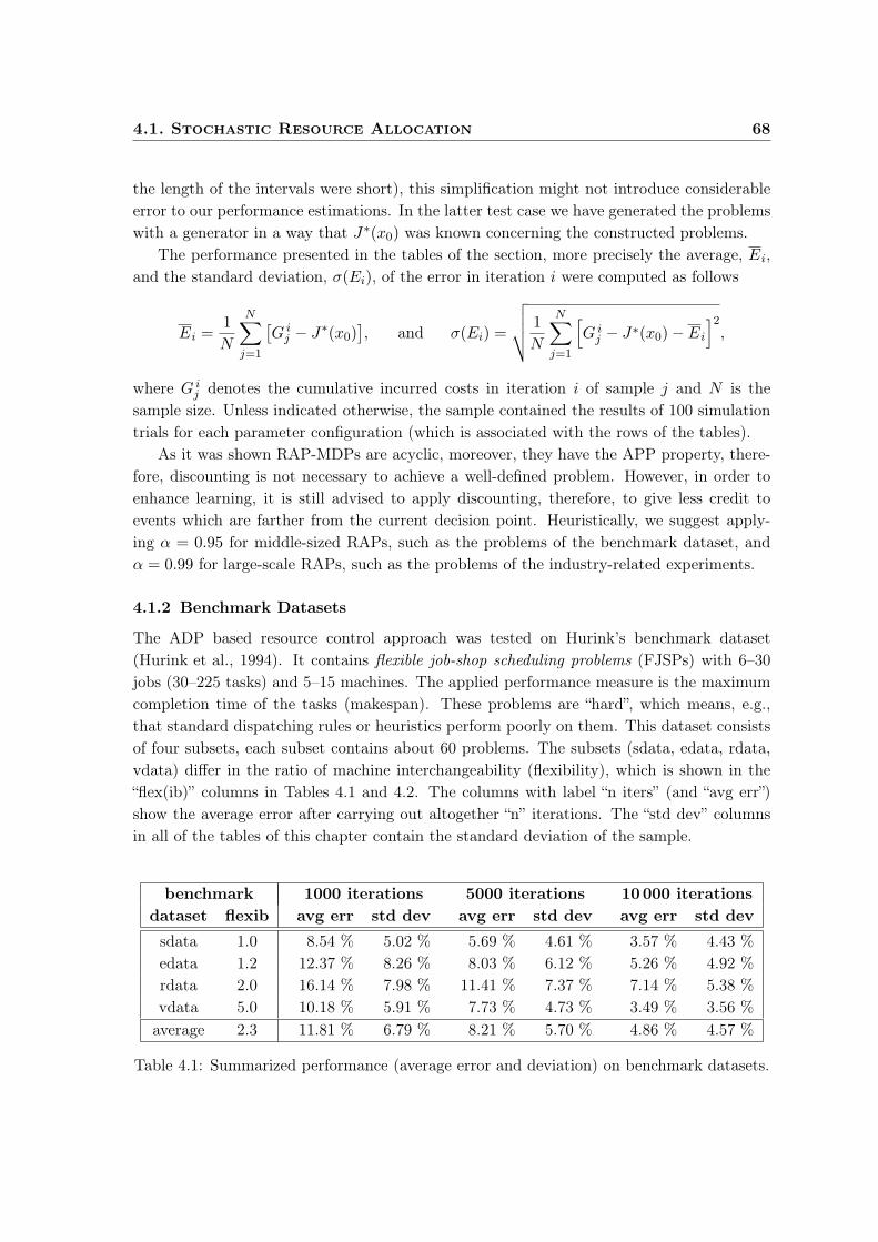
4.1. Stochastic Resource Allocation 68
the length of the intervals were short), this simplification might not introduce considerableerror to our performance estimations. In the latter test case we have generated the problemswith a generator in a way that J∗(x0) was known concerning the constructed problems.
The performance presented in the tables of the section, more precisely the average, Ei,and the standard deviation, σ(Ei), of the error in iteration i were computed as follows
Ei =1
N
N∑
j=1
[G i
j − J∗(x0)], and σ(Ei) =
√√√√ 1
N
N∑
j=1
[G i
j − J∗(x0) − Ei
]2,
where G ij denotes the cumulative incurred costs in iteration i of sample j and N is the
sample size. Unless indicated otherwise, the sample contained the results of 100 simulationtrials for each parameter configuration (which is associated with the rows of the tables).
As it was shown RAP-MDPs are acyclic, moreover, they have the APP property, there-fore, discounting is not necessary to achieve a well-defined problem. However, in order toenhance learning, it is still advised to apply discounting, therefore, to give less credit toevents which are farther from the current decision point. Heuristically, we suggest apply-ing α = 0.95 for middle-sized RAPs, such as the problems of the benchmark dataset, andα = 0.99 for large-scale RAPs, such as the problems of the industry-related experiments.
4.1.2 Benchmark Datasets
The ADP based resource control approach was tested on Hurink’s benchmark dataset(Hurink et al., 1994). It contains flexible job-shop scheduling problems (FJSPs) with 6–30jobs (30–225 tasks) and 5–15 machines. The applied performance measure is the maximumcompletion time of the tasks (makespan). These problems are “hard”, which means, e.g.,that standard dispatching rules or heuristics perform poorly on them. This dataset consistsof four subsets, each subset contains about 60 problems. The subsets (sdata, edata, rdata,vdata) differ in the ratio of machine interchangeability (flexibility), which is shown in the“flex(ib)” columns in Tables 4.1 and 4.2. The columns with label “n iters” (and “avg err”)show the average error after carrying out altogether “n” iterations. The “std dev” columnsin all of the tables of this chapter contain the standard deviation of the sample.
benchmark 1000 iterations 5000 iterations 10000 iterations
dataset flexib avg err std dev avg err std dev avg err std dev
sdata 1.0 8.54 % 5.02 % 5.69 % 4.61 % 3.57 % 4.43 %edata 1.2 12.37 % 8.26 % 8.03 % 6.12 % 5.26 % 4.92 %rdata 2.0 16.14 % 7.98 % 11.41 % 7.37 % 7.14 % 5.38 %vdata 5.0 10.18 % 5.91 % 7.73 % 4.73 % 3.49 % 3.56 %
average 2.3 11.81 % 6.79 % 8.21 % 5.70 % 4.86 % 4.57 %
Table 4.1: Summarized performance (average error and deviation) on benchmark datasets.

4.1. Stochastic Resource Allocation 69
In Table 4.1 the summarized performance on the benchmark datasets is shown. Table4.2 illustrates the performance on some typical dataset instances and also gives some detailson them, e.g., the number of machines and jobs (columns with labels “mcs” and “jbs”).
benchmark configuration average error (standard deviation)
dataset inst mcs jbs flex 1000 iters 5000 iters 10000 iters
sdata mt06 6 6 1 1.79 (1.01) % 0.00 (0.00) % 0.00 (0.00) %sdata mt10 10 10 1 9.63 (4.59) % 8.83 (4.37) % 7.92 (4.05) %sdata la09 5 15 1 5.67 (2.41) % 3.87 (1.97) % 3.05 (1.69) %sdata la19 10 10 1 11.65 (5.21) % 6.44 (3.41) % 3.11 (1.74) %sdata la39 15 15 1 14.61 (7.61) % 12.74 (5.92) % 11.92 (5.63) %sdata la40 15 15 1 10.98 (5.04) % 8.87 (4.75) % 8.39 (4.33) %edata mt06 6 6 1.15 0.00 (0.00) % 0.00 (0.00) % 0.00 (0.00) %edata mt10 10 10 1.15 18.14 (8.15) % 12.51 (6.12) % 9.61 (4.67) %edata la09 5 15 1.15 7.51 (3.33) % 5.23 (2.65) % 2.73 (1.89) %edata la19 10 10 1.15 8.04 (4.64) % 4.14 (2.81) % 1.38 (1.02) %edata la39 15 15 1.15 22.80 (9.67) % 17.32 (8.29) % 12.41 (6.54) %edata la40 15 15 1.15 14.78 (7.14) % 8.08 (4.16) % 6.68 (4.01) %rdata mt06 6 6 2 6.03 (3.11) % 0.00 (0.00) % 0.00 (0.00) %rdata mt10 10 10 2 17.21 (8.21) % 12.68 (6.81) % 7.87 (4.21) %rdata la09 5 15 2 7.08 (3.23) % 6.15 (2.92) % 3.80 (2.17) %rdata la19 10 10 2 18.03 (8.78) % 11.71 (5.78) % 8.87 (4.38) %rdata la39 15 15 2 24.55 (9.59) % 18.90 (8.05) % 13.06 (7.14) %rdata la40 15 15 2 23.90 (7.21) % 18.91 (6.92) % 14.08 (6.68) %vdata mt06 6 6 3 0.00 (0.00) % 0.00 (0.00) % 0.00 (0.00) %vdata mt10 10 10 5 8.76 (4.65) % 4.73 (2.23) % 0.45 (0.34) %vdata la09 5 15 2.5 9.92 (5.32) % 7.97 (3.54) % 4.92 (2.60) %vdata la19 10 10 5 14.42 (7.12) % 11.61 (5.76) % 6.54 (3.14) %vdata la39 15 15 7.5 16.16 (7.72) % 12.25 (6.08) % 9.02 (4.48) %vdata la40 15 15 7.5 5.86 (3.11) % 4.08 (2.12) % 2.43 (1.83) %
Table 4.2: Performance (average error and deviation) on some typical benchmark problems.
The best performance was achieved by (Mastrolilli and Gambardella, 2000) on thesebenchmark FJSP datasets. Though, their algorithm performs slightly better than ours,their solution exploits the (unrealistic) specialties of the dataset, e.g., the durations do notdepend on the resources; the tasks are linearly ordered in the jobs; each job consists ofthe same number of tasks. Moreover, it cannot be easily generalized to stochastic resourcecontrol problem our algorithm faces. Therefore, the comparison of the two solutions is hard.

4.1. Stochastic Resource Allocation 70
4.1.3 Distributed Sampling
The possible parallelizations of the presented method was also investigated, i.e., the speedup
of the system relative to the number of processors (in practise, the multiprocessor envi-ronment was emulated on a single processor, only). The average number of iterations wasstudied, until the system could reach a solution with less than 5% error on Hurink’s dataset.The average speed of a single processor was treated as a unit, for comparison.
In Figure 4.1 two cases are shown: in the first case (rear dark bars) each processor couldaccess a common global value function. It means that each processor could read and writethe same global value function, but otherwise, they searched (sampled the search space)independently. Figure 4.1 demonstrates that in this case the speedup was almost linear.
Figure 4.1: Average speedup relative to the number of processors.
In the second case (front light bars) each processor had its own (local) value function(which is more realistic in a strongly distributed system, such as a GRID) and, after thesearch had been finished, these individual value functions were compared. Therefore, all ofthe processors had estimations of their own, and after the search, the local solution of thebest performing processor was selected. Figure 4.1 shows the achieved speedup in case westopped the simulation if any of the processors achieved a solution with less than 5% error.
The experiments show that the computation of the resource allocator function can beeffectively distributed, even if there is not a commonly accessible value function available.
4.1.4 Industry Related Tests
We also initiated numerical experiments on a simulated factory by modeling the structure ofa real plant producing customized mass-products, especially, light bulbs. These industrialdata came from a huge national industry-academia project for research and developmentof solutions which support manufacturing enterprises in coping with the requirements ofadaptiveness, realtimeness and cooperativeness (Monostori et al., 2008).
Since, we did not have access to historical data concerning past orders, we used randomlygenerated orders (jobs) with random due dates. The tasks and the process-plans of the jobs,however, covered real products; as well as, the resources covered real machine types. Inthis plant the machines require product-type dependent setup times, and there are some
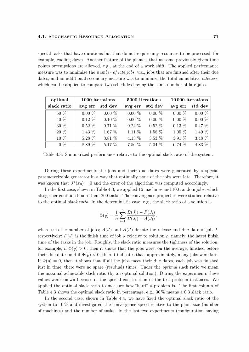
4.1. Stochastic Resource Allocation 71
special tasks that have durations but that do not require any resources to be processed, forexample, cooling down. Another feature of the plant is that at some previously given timepoints preemptions are allowed, e.g., at the end of a work shift. The applied performancemeasure was to minimize the number of late jobs, viz., jobs that are finished after their duedates, and an additional secondary measure was to minimize the total cumulative lateness,which can be applied to compare two schedules having the same number of late jobs.
optimal 1000 iterations 5000 iterations 10000 iterations
slack ratio avg err std dev avg err std dev avg err std dev
50 % 0.00 % 0.00 % 0.00 % 0.00 % 0.00 % 0.00 %40 % 0.12 % 0.10 % 0.00 % 0.00 % 0.00 % 0.00 %30 % 0.52 % 0.71 % 0.24 % 0.52 % 0.13 % 0.47 %20 % 1.43 % 1.67 % 1.11 % 1.58 % 1.05 % 1.49 %10 % 5.28 % 3.81 % 4.13 % 3.53 % 3.91 % 3.48 %0 % 8.89 % 5.17 % 7.56 % 5.04 % 6.74 % 4.83 %
Table 4.3: Summarized performance relative to the optimal slack ratio of the system.
During these experiments the jobs and their due dates were generated by a specialparameterizable generator in a way that optimally none of the jobs were late. Therefore, itwas known that J∗(x0) = 0 and the error of the algorithm was computed accordingly.
In the first case, shown in Table 4.3, we applied 16 machines and 100 random jobs, whichaltogether contained more than 200 tasks. The convergence properties were studied relativeto the optimal slack ratio. In the deterministic case, e.g., the slack ratio of a solution is
Φ(%) =1
n
n∑
i=1
B(Ji) − F (Ji)
B(Ji) −A(Ji),
where n is the number of jobs; A(J) and B(J) denote the release and due date of job J ,respectively; F (J) is the finish time of job J relative to solution %, namely, the latest finishtime of the tasks in the job. Roughly, the slack ratio measures the tightness of the solution,for example, if Φ(%) > 0, then it shows that the jobs were, on the average, finished beforetheir due dates and if Φ(%) < 0, then it indicates that, approximately, many jobs were late.If Φ(%) = 0, then it shows that if all the jobs meet their due dates, each job was finishedjust in time, there were no spare (residual) times. Under the optimal slack ratio we meanthe maximal achievable slack ratio (by an optimal solution). During the experiments thesevalues were known because of the special construction of the test problem instances. Weapplied the optimal slack ratio to measure how “hard” a problem is. The first column ofTable 4.3 shows the optimal slack ratio in percentage, e.g., 30% means a 0.3 slack ratio.
In the second case, shown in Table 4.4, we have fixed the optimal slack ratio of thesystem to 10 % and investigated the convergence speed relative to the plant size (numberof machines) and the number of tasks. In the last two experiments (configuration having
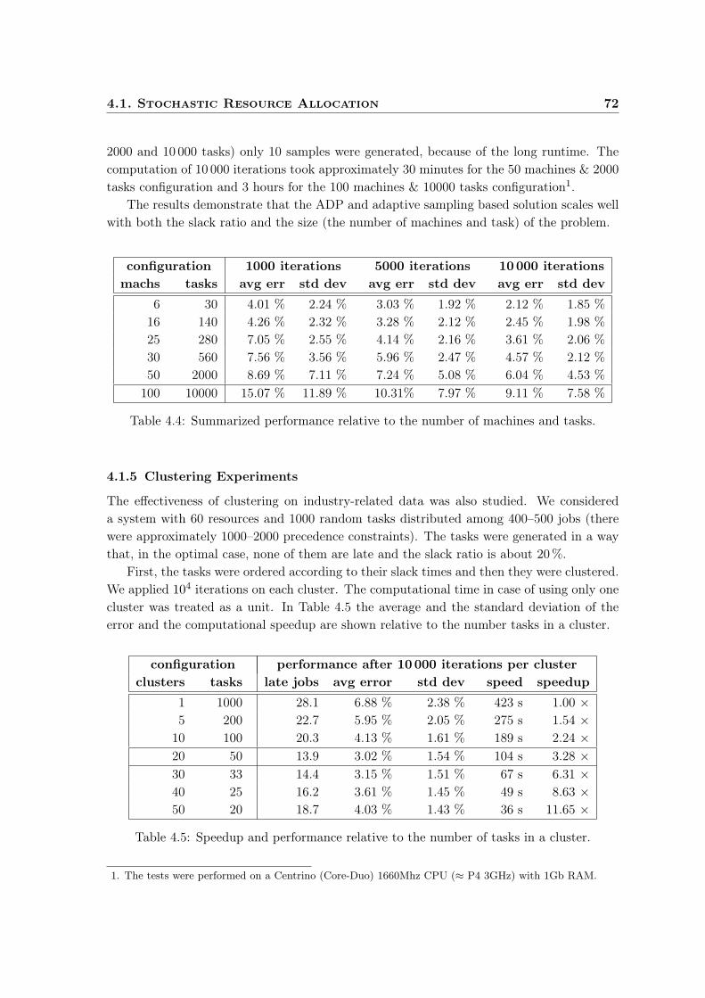
4.1. Stochastic Resource Allocation 72
2000 and 10 000 tasks) only 10 samples were generated, because of the long runtime. Thecomputation of 10 000 iterations took approximately 30 minutes for the 50 machines & 2000tasks configuration and 3 hours for the 100 machines & 10000 tasks configuration1.
The results demonstrate that the ADP and adaptive sampling based solution scales wellwith both the slack ratio and the size (the number of machines and task) of the problem.
configuration 1000 iterations 5000 iterations 10000 iterations
machs tasks avg err std dev avg err std dev avg err std dev
6 30 4.01 % 2.24 % 3.03 % 1.92 % 2.12 % 1.85 %16 140 4.26 % 2.32 % 3.28 % 2.12 % 2.45 % 1.98 %25 280 7.05 % 2.55 % 4.14 % 2.16 % 3.61 % 2.06 %30 560 7.56 % 3.56 % 5.96 % 2.47 % 4.57 % 2.12 %50 2000 8.69 % 7.11 % 7.24 % 5.08 % 6.04 % 4.53 %
100 10000 15.07 % 11.89 % 10.31% 7.97 % 9.11 % 7.58 %
Table 4.4: Summarized performance relative to the number of machines and tasks.
4.1.5 Clustering Experiments
The effectiveness of clustering on industry-related data was also studied. We considereda system with 60 resources and 1000 random tasks distributed among 400–500 jobs (therewere approximately 1000–2000 precedence constraints). The tasks were generated in a waythat, in the optimal case, none of them are late and the slack ratio is about 20%.
First, the tasks were ordered according to their slack times and then they were clustered.We applied 104 iterations on each cluster. The computational time in case of using only onecluster was treated as a unit. In Table 4.5 the average and the standard deviation of theerror and the computational speedup are shown relative to the number tasks in a cluster.
configuration performance after 10000 iterations per cluster
clusters tasks late jobs avg error std dev speed speedup
1 1000 28.1 6.88 % 2.38 % 423 s 1.00 ×
5 200 22.7 5.95 % 2.05 % 275 s 1.54 ×
10 100 20.3 4.13 % 1.61 % 189 s 2.24 ×
20 50 13.9 3.02 % 1.54 % 104 s 3.28 ×
30 33 14.4 3.15 % 1.51 % 67 s 6.31 ×
40 25 16.2 3.61 % 1.45 % 49 s 8.63 ×
50 20 18.7 4.03 % 1.43 % 36 s 11.65 ×
Table 4.5: Speedup and performance relative to the number of tasks in a cluster.
1. The tests were performed on a Centrino (Core-Duo) 1660Mhz CPU (≈ P4 3GHz) with 1Gb RAM.
4.2. Varying Environments 73
The results demonstrate that partitioning the search space not only results in a greaterspeed, but it is often accompanied by better solutions. The latter phenomenon can be ex-plained by the fact that using smaller sample trajectories generates smaller variance that ispreferable for learning. On the other hand, making too small clusters may decrease the per-formance (e.g., making 50 clusters with 20 tasks in the current case). In our particular caseapplying 20 clusters with approximately 50 tasks in each cluster balances good performance(3.02% error on the average) with remarkable speedup (approximately 3.28×).
As clustering the tasks represents a considerable help in dealing with large-scale RAPs,their further theoretical and experimental investigation would be very promising.
4.2 Varying Environments
In this section we present two numerical experiments. The first one demonstrates the effectsof environmental changes during Q-learning based scheduling. The second one presents aparameter analysis concerning the effectiveness of SARSA in (ε, δ)-type grid world domains.
4.2.1 Adaptation to Disturbances
In order to verify the algorithm in changing environments, experiments were carried outon random JSPs with the aim of minimizing the makespan. The adaptive features of thesystem were tested by confronting it with unexpected events, such as: resource breakdowns,new resource availability (Figure 4.2), new job arrivals or job cancellations (Figure 4.3). InFigures 4.2 and 4.3 the horizontal axis represents time, while the vertical one, the achievedperformance measure. The figures were made by averaging hundred random samples. Inthese tests 20 machines were used with few dozens of jobs. In each case there was an unex-pected event at time t = 100. After the change took place, we considered two possibilities:we either restarted the iterative scheduling process from scratch or continued the learning,using the current (obsolete) value function. We experienced that the latter approach is muchmore efficient. This was one of the reasons why we started to study how the value functionof a control policy depends on the dynamics of the underlying Markov process.
The results, black curves, show the case when the obsolete value function approximationwas applied after the change took place. The performance which would arise if the systemrecomputed the whole schedule from scratch is drawn in gray in part (a) of Figure 4.2.
One can notice that even if the problem became “easier” after the change in the environ-ment (at time t = 100), for example, a new resource was available (part (b) of Figure 4.2)or a job was cancelled (part (b) of Figure 4.3), the performance started to slightly decrease(κ started to slightly increase) after the event. This phenomena can be explained by thefact that even in these special cases the system had to “explore” the new configuration.
Recall that Theorems 9 and 11 measure the amount of the possible change in the valuefunction of a control policy in case there were changes in the MDP, but since they applysupremum norm, they only provide bounds for worst case situations. However, the results ofour numerical experiments, shown in Figures 4.2 and 4.3, are indicative of the phenomenon

4.2. Varying Environments 74
that in an average case the change is much less. Therefore, applying the obsolete valuefunction after a change took place is preferable over restarting the optimization from scratch.
170
190
210
230
250
270
290
310
330
1 20 40 60 80 100 120 140 160 180
170
190
210
230
250
270
290
310
330
1 20 40 60 80 100 120 140 160 180 200 200
t ~ t ~time time
k(t) k(t)
(a) (b)
k’(t)
Figure 4.2: The black curves, κ(t), show the performance measure in case there was a re-source breakdown (a) or a new resource availability (b) at t = 100; the graycurve, κ’(t), illustrates the case the policy would be recomputed from scratch.
200
220
240
260
280
300
320
340
360
1 20 40 60 80 100 120 14060 80 100 120 140 160 180 200
k(t)
(a) (b)
t ~ t ~time time
160 180
200
220
240
260
280
300
320
340
360
1 20 40 200
k(t)
Figure 4.3: The black curves, κ(t), show the performance measure during resource controlin case there was a new job arrival (a) or a job cancellation (b) at time t = 100.
4.2.2 Varying Grid Worlds
We also performed numerical experiments on a variant of the classical grid world problem(Sutton and Barto, 1998). The original version of this problem can be briefly described asfollows: an agent wanders in a rectangular world starting from a random initial state withthe aim of finding the goal state. In each state the agent is allowed to choose from fourpossible actions: “north”, “south”, “east” and “west”. After an action was selected, the agentmoves one step in that direction. There are some mines on the field, as well, that the agentshould avoid. An episode ends if the agent finds the goal state or hits a mine. Duringour experiments, we have applied randomly generated 10 × 10 grid worlds (therefore, theseMDPs had 100 states) with 10 mines. The (immediate) cost of taking a (non-terminating)step was 5, a cost of hitting a mine was 100 and the cost of finding the goal state was −100.

4.2. Varying Environments 75
In order to perform the experiment described by Table 4.6, we applied the “RL-Glue”framework2 which consists of open source softwares and aims at being a standard protocolfor benchmarking and interconnecting reinforcement learning agents and environments.
We have analyzed an (ε, δ)-type version of grid world, where the problem formed an(ε, δ)-MDP. More precisely, we have investigated the case when for all time t, the transition-probabilities could vary by at most ε ≥ 0 around the base transition-probability values andthe immediate-costs could vary by at most δ ≥ 0 around the base cost values.
During our numerical experiments, the environment changed at each time-step. Thesechanges were generated as follows. First, changes concerning the transition-probabilities aredescribed. In our randomized grid worlds the agent was taken to a random surroundingstate (no matter what action it chose) with probability η and this probability changed aftereach step. The new η was computed according to the uniform distribution, but its possiblevalues were bounded by the values described in the first row of Table 4.6.
Similarly, the immediate-costs of the base MDP (cf. the first paragraph) were perturbed
with a uniform random variable that changed at each time-step. Again, its (absolute) valuewas bounded by δ, which is presented in the first column of the table. The values shownwere divided by 100 to achieve the same scale as the transition-probabilities have.
∆ ‖g‖ the bounds for the varying probability of arriving at random states ∼ ε
δ/100 0.0 0.1 0.2 0.3 0.4 0.5 0.6 0.7 0.8 0.9 1.0
0.0 -55.5 -48.8 -41.4 -36.7 -26.7 -16.7 -8.5 2.1 14.2 31.7 46.00.1 -54.1 -46.1 -41.2 -34.5 -25.8 -15.8 -6.0 3.7 16.5 32.3 46.30.2 -52.5 -44.8 -40.1 -34.4 -25.3 -15.4 -5.8 4.0 17.6 33.1 48.10.3 -49.7 -42.1 -36.3 -31.3 -23.9 -14.2 -5.3 8.0 18.1 37.2 51.60.4 -47.4 -41.5 -34.7 -30.7 -22.2 -12.2 -2.3 8.8 20.2 38.3 52.00.5 -42.7 -41.0 -34.5 -24.8 -21.1 -10.1 -1.3 11.2 25.7 39.2 52.10.6 -36.1 -36.5 -29.7 -24.0 -16.8 -7.9 1.1 17.0 31.3 43.9 54.10.7 -30.2 -29.3 -29.3 -19.1 -13.4 -6.0 7.4 18.9 26.9 47.2 60.90.8 -23.1 -27.0 -21.4 -18.8 -10.9 -2.6 8.9 22.5 31.3 50.0 64.20.9 -14.1 -19.5 -21.0 -12.4 -7.5 0.7 13.2 23.2 38.9 52.2 68.11.0 -6.8 -10.7 -14.5 -7.1 -5.3 6.6 15.7 26.4 39.8 57.3 68.7
Table 4.6: The (average) cumulative costs gathered by SARSA in varying grid worlds.
Table 4.6 was generated using an (optimistic) SARSA algorithm, namely, the actual pol-icy was evaluated by SARSA, then the policy was (optimistically) improved, more precisely,the greedy policy with respect to the achieved evaluation was calculated. That policy wasalso soft, namely, it made random explorations with probability 0.05. We have generated1000 random grid worlds for each parameter pairs and performed 10 000 episodes in each of
2. http://rlai.cs.ualberta.ca/RLBB/top.html

4.2. Varying Environments 76
these generated worlds. The results presented in the table were calculated by averaging thecumulative costs over all episodes and over all generated sample worlds.
The parameter analysis shown in Table 4.6 is indicative of the phenomenon that changesin the transition-probabilities have a much higher impact on the performance. Even largeperturbations in the costs were tolerated by SARSA, but large variations in the transition-probabilities caused a high decrease in the performance. An explanation could be that largechanges in the transitions cause the agent to loose control over the events, since it becomesvery hard to predict the effects of the actions and, hence, to estimate the expected costs.
Chapter 5
Conclusion
Efficient allocation of scarce, reusable resources over time to interconnected tasks is animportant problem that arises in many “real world” domains. Though, in the past decadesmuch effort was spent on designing efficient resource allocation algorithms, most of theseapproaches investigated deterministic and static problems. However, in practise there is asignificant amount of uncertainty concerning resource allocation, for example, the executiontimes of the tasks are usually not known exactly. Moreover, there could be disturbancesand changes in the environment, as well. These issues seriously limit the applicability ofclassical solution methods. Unfortunately, it is not trivial the extend these algorithms, suchas branch and cut or constraint satisfaction, to handle stochastic problems. Instead of thisdirection, the thesis took a machine learning (ML) approach to resource allocation to facethese additional challenges. In this concluding chapter we briefly summarize the solutionconcerning both managing uncertainties during resource allocation and dealing with thechanges of the environment. We also take the opportunity to highlight a few advantages ofthe approach and, finally, we present some possible further research directions, as well.
5.1 Managing Uncertainties
In order to define an efficient reactive solution, first, a general resource allocation frameworkwas presented and it was reformulated as a stochastic shortest path problem, a specialMarkov decision process (MDP). It was shown that this reformulation has several favorableproperties, such as it has finite state and action spaces, it is acyclic, hence all policies areproper and the space of control policies can be safely restricted. The possibility of achievingproactive solutions with this approach was also investigated and proactive solutions wereformulated as control policies of suitably defined partially observable MDPs (POMDPs).
The core idea of the proposed solution was the application of simulation based rein-forcement learning (RL) techniques together with other machine learning methods. Theexploration and exploitation ratio of the system was controlled by a Boltzmann formula,combined with a Metropolis algorithm. Regarding value function representations, two ap-proaches were studied: hash table and support vector regression (SVR). Afterwards, severaladditional improvements, such as the application of rollout algorithms, action space de-
77
5.2. Dealing with Changes 78
composition, task clustering and distributed sampling, were suggested for speeding up thecomputation of a good policy. Finally, the effectiveness of the approach was demonstratedby results of simulation experiments on both benchmark and industry-related data.
There are several advantages why ML based resource allocation is preferable to otherkinds of RAP solutions, e.g., classical approaches. These favorable features are as follows:
1. The presented RAP framework is very general, it can model several resource manage-ment problems that appear in practise, such as scheduling problems, transportationproblems, inventory management problems or maintenance and repair problems.
2. RL based methods essentially face the problem under the presence of uncertainties,since their theoretical foundation is provided by MDPs. Moreover, they can adapt tounexpected changes in the environmental dynamics, such as breakdowns.
3. Additionally, for most algorithms theoretical guarantees of finding (approximately)optimal solutions, at least in the limit, are known. As demonstrated by our experi-ments, the actual convergence speed for RAPs is usually high, especially in the case ofapplying the described improvements, such as clustering or distributed sampling.
4. The simulation experiments on industrial data also demonstrate that RL based solu-tions scale well with the workload and the size of the problem and, therefore, they canbe effectively applied to handle real world problems, such as production control.
5. Domain specific knowledge can also be incorporated into the solution. The base policyof the rollout algorithm, for example, can reflect a priori knowledge about the structureof the problem; later this knowledge may appear in the exploration strategy.
6. Finally, the proposed method constitutes an any-time solution, since the sampling canbe stopped after any number of iterations. By this way, the amount of computationaltime can be controlled, which is also an important practical advantage.
Consequently, ML approaches have great potentials in dealing with real world RAPs, sincethey can handle large-scale problems even in dynamic and uncertain environments.
5.2 Dealing with Changes
The theory of MDPs provide a general framework for modeling decision making in stochasticdynamic systems, if we know a function that describes the dynamics or we can simulate it,for example, with a suitable program. In some situations, however, the dynamics of thesystem may change, too. In theory, this change can be modeled with another (higher level)MDP, as well, but doing so would lead to models which are practically intractable.
In the dissertation we have argued that the value function of a (stationary, Marko-vian, randomized) control policy in a (discounted or acyclic undiscounted) MDP Lipschitzcontinuously depends on the transition-probability function and the immediate-cost func-tion, therefore, small changes in the environment result only in small changes in the value
5.3. Further Research Directions 79
function. A similar result was already known for optimal value functions in the case oftransition-probabilities, but we have presented an improved estimation for that case, aswell. A bound for changes in the discount factor was also proven, and it was demonstratedthat this dependence was not Lipschitz continuous. Additionally, it was proven that changesin the discount rate could be traced back to changes in the cost function. Though, optimalpolicies may also change if the environment had changed, we showed that the previous re-sults can be extended to optimal value functions, as well. The application of the Lipschitzproperty helps the theoretical treatment of changing environments or inaccurate models,e.g., if the transition-probabilities or the immediate-costs are estimated statistically, only.
In order to theoretically analyze environmental changes, the framework of (ε, δ)-MDPswas introduced as a generalization of classical MDPs and ε-MDPs. In this quasi-stationarymodel the transition-probability function and the immediate-cost function may change overtime, but the cumulative changes must remain bounded by ε and δ, asymptotically.
Afterwards, we have investigated how RL methods could work in this kind of changingenvironment. We have presented a general theorem that estimated the asymptotic distanceof a value function sequence from a fixed value function. This result was applied to deducea convergence theorem for value function based algorithms that work in (ε, δ)-MDPs.
In order to demonstrate our approach, we have presented some numerical experiments,too. First, two simple iterative processes were shown, a “well-behaving” stochastic processand a “pathological”, oscillating deterministic process. Later, the effects of environmentalchanges on Q-learning based flexible job-shop scheduling was experimentally studied. Fi-nally, we have analyzed how SARSA could work in varying (ε, δ)-type grid world domains.
We can conclude that value function based RL algorithms can work in varying envi-ronments, at least if the changes remain bounded in the limit. The asymptotic distance ofthe generated value function sequence from the optimal value function of base MDP of thechanging environment is bounded for a large class of stochastic iterative algorithms. More-over, this bound is proportional to the diameter of this set, e.g., to parameters ε and δ inthe case of (ε, δ)-MDPs. These results were illustrated through three classical RL methods:asynchronous value iteration, Q-learning and temporal difference learning policy evaluation.
5.3 Further Research Directions
Several further research directions are possible to enhance the proposed ML based resourceallocation approach. Now, as a conclusion to the thesis, we highlight some of them.
The suggested improvements, such as clustering and distributed sampling, should be fur-ther investigated, both theoretically and experimentally, since they resulted in considerablespeedup. The guidance of reinforcement learning with rollout algorithms might be effectivelyapplied in other applications, as well. Regarding proactive solutions, efficient algorithms tohandle partially observable MDPs (POMDPs) should also be studied. The theoretical anal-ysis of the average effects of environmental changes on the value functions of a policy couldresult in new approaches to handle disturbances. Another promising direction would be toextend the solution in a way which also takes risk into account and, for example, minimizes

5.3. Further Research Directions 80
not only the expected value of the total costs but also the deviation, as a secondary opti-mization criterion. Finally, trying to apply the solution in a pilot project to control a realplant would be interesting and could motivate many more further research directions.
Concerning changes in the dynamics, a promising direction could be to investigate en-vironments with non-bounded changes, e.g., when the environment might drift over time.Naturally, this drift should also be sufficiently slow in order to give the opportunity to thelearning algorithm to track the changes. Another possible direction could be the analysis ofthe convergence results in case of applying value function approximation. The classical prob-lem of exploration and exploitation should also be reinvestigated in changing environments.Finally, finding finite time bounds for the convergence of stochastic iterative algorithms for(a potentially restricted class of) non-stationary environments would also be important.
Appendix: Proofs
In this appendix we present the proofs of all theorems and lemmas we gave. Naturally, wedo not prove those statements which were taken from other sources. In the latter casesadequate references are given in the text concerning the locations of the proofs.
Theorem 7 Consider a POMDP and its fully observable MDP counterpart, which system has
the same state space, action space, transition-probabilities and costs as the original POMDP,
only the observability is different. The optimal cost-to-go functions of the POMDP and the
MDP are denoted by J∗ and J∗, respectively. Then, for all belief state b, we have
∑
x∈X
b(x)J∗(x) ≤ J∗(b) ≤∑
x∈X
b(x)J∗(x) +c
1 − α,
where c = (gmax − gmin); gmax = maxg(x, a) | x ∈ X, a ∈ A and similarly for gmin. If the
immediate-cost function g is not constant (c 6= 0), then the second inequality is strict.
Proof We will prove the theorem in two steps. First, we will show that for all belief states,∑x∈X
b(x)J∗(x) ≤ J∗(b), then we will prove that J∗(b) ≤∑
x∈Xb(x)J∗(x) + c/(1 − α),
where c = (gmax − gmin). The first part of the theorem will be proven by induction. We cantreat our infinite horizon problem as the limit of the finite horizon problems and, thus, wecan apply induction on the horizon. The Bellman equation for the N -stage problem is
J∗k+1(x) = min
a∈A(x)
g(x, a) + α
∑
y∈X
p(y | x, a)J∗k (y)
, (5.1)
for all k ∈ 0, . . . , N − 1 and x ∈ X. Note that J∗0 = 0 by definition (we do not have to
consider terminal cost). It is known, (see Bertsekas and Tsitsiklis, 1996), that for all x ∈ X
J∗(x) = J∗∞(x) = lim
N→∞J∗
N (x) (5.2)
It is obvious that∑
x∈XJ∗
N (x) b(x) ≤ J∗N (b) holds if N = 0, since J∗
0 ≡ J∗0 ≡ 0 (they are
both constant zero functions). Now, we assume that it holds for N and prove it for N + 1:
J∗N+1(b) = min
a∈A
g(b, a) + α
∑
z∈O
p(z | b, a) J∗N (τ(b, a, z))
≥
81

Appendix: Proofs 82
≥ mina∈A
g(b, a) + α
∑
z∈O
p(z | b, a)∑
y∈X
τ(b, a, z)(y)J∗N (y)
=
= mina∈A
∑
x∈X
b(x) g(x, a) + α∑
z∈O
p(z | b, a)∑
y∈X
∑x∈X
p(z, y | x, a) b(x)
p(z | b, a)J∗
N (y)
=
= mina∈A
∑
x∈X
b(x) g(x, a) + α∑
z∈O
∑
y∈X
∑
x∈X
p(z, y | x, a) b(x)J∗N (y)
=
= mina∈A
∑
x∈X
b(x)
g(x, a) + α
∑
z∈O
∑
y∈X
p(z | y, a) p(y | x, a)J∗N (y)
=
= mina∈A
∑
x∈X
b(x)
g(x, a) + α
∑
y∈X
p(y | x, a)J∗N (y)
≥
now, we apply Jensen’s inequality with the remark that min is a concave function
≥∑
x∈X
b(x)mina∈A
g(x, a) + α
∑
y∈X
p(y | x, a)J∗N (y)
=
∑
x∈X
b(x)J∗N+1(x)
for all b ∈ B. Now, we turn to the second part of the theorem and show that for allb ∈ B : J∗(b) ≤
∑x∈X
b(x)J∗(x) + (gmax − gmin)/(1 − α). In possession of the knowl-edge that the first part of the theorem holds, the second part can be proven as follows.We can notice that at each step the maximum difference of the incurred cost between theconvex combination of the optimal cost-to-go functions of the fully observable and the non-observable (belief state) MDPs (that also uses a convex combination for cost) is gmax−gmin,which is denoted by c and it is discounted by α. This simply builds a geometric series:c+αc+α2c+ · · · = c/(1−α). To show that this inequality is strict, suppose (indirectly) thatJ∗(b) =
∑x b(x)J
∗(x)+ c/(1−α). It means that, at each step the difference is gmax−gmin,even at the first step. Thus, it must be the case that
∑x J
∗1 (x) b(x) = gmin, therefore, for all
state x such that b(x) 6= 0 there must be an action a such that g(x, a) = gmin. Additionally,in order to satisfy the equality, J∗
1 (b) = gmax must hold. It means that the best actiona in b has the cost g(b, a) =
∑x b(x) g(x, a) = gmax, which cannot be the best action (if
c 6= 0), since for each state x (such that b(x) 6= 0) there is an action a that has minimalcost, g(x, a) = gmin. We have reached a contradiction, therefore, the inequality is strict.
Lemma 8 (1) There exists a POMDP and a corresponding fully observable MDP such that,
for a belief state b: J∗(b) = 〈J∗, b〉; (2) for all ε > 0 there exists a POMDP and a corre-
sponding MDP such that for a belief state b: |J∗(b) − 〈J∗, b〉 − c/(1 − α)| < ε.
Proof The lemma is trivial if constant immediate-cost functions are allowed. Let usnow assume that we have a non-constant cost function. We can also assume, without loss
Appendix: Proofs 83
of generality, that gmin = 0 and gmax = 1. Then, the first statement of the lemma isstill straightforward to prove, since any POMDP which is deterministic or which is fullyobservable (e.g., the observations are the real states) can do with a b ∈ B such that b(x) = 1
for an x ∈ X. If the system is deterministic, then this result is valid for NOMDPs, as well.The second part of the lemma can be shown through an example, moreover, the applied
POMDP will be a NOMDP (viz., its observation space contains only one element). Considera NOMDP with X = x1, . . . , xn, A = a1, . . . , an, for all xi : A(xi) = a1, . . . , an. Forall xi and aj the immediate-cost g(xi, aj) = 0 if i = j and g(xi, aj) = 1 otherwise. Thetransition-probabilities for all x, y ∈ X and a ∈ A: p(y | x, a) = 1/n. Then, if the systemwas fully observable, the optimal cost-to-go function would be J∗(x) = 0 for all x ∈ X,because in each state xi one could choose an action (ai) that did not have any cost. How-ever, consider a belief state b such that b(x) = 1/n for all x ∈ X. In this case for eachaction a ∈ A its immediate-cost is g(b, a) =
∑x b(x)g(x, a) = (n − 1)/n, therefore, the
optimal control policy in b also incur (n − 1)/n cost before it arrives back to belief stateb. In the long run, J∗(b) = (1/(1 − α)) · ((n − 1)/n). Because c = (gmax − gmin) = 1 andfor any ε > 0 we can choose a large enough n such that 1 − (n − 1)/n < ε, consequently,J∗(b) can be arbitrary close to 〈J∗, b〉+c/(1−α) = 1/(1−α). Thus, we proved both parts.
Theorem 9 Assume that two discounted MDPs, M1 and M2, differ only in their transition-
probability functions, and let these two functions be denoted by p1 for M1 and p2 for M2.
Let the value functions of a (stationary, Markovian, randomized) control policy π be denoted
by Jπ1 related to M1 and Jπ
2 related to M2. Then, the following inequality holds
‖Jπ1 − Jπ
2 ‖∞ ≤α |X| ‖g‖∞(1 − α)2
‖p1 − p2‖∞ .
Proof Using the Bellman equation in the first step, the absolute value of the difference ofthe two cost-to-go functions in any state can be estimated as follows
∀x ∈ X : |Jπ1 (x) − Jπ
2 (x)| =
=
∣∣∣∣∣∣
∑
a∈A(x)
π(x, a)[g(x, a) + α
∑
y∈X
p1(y | x, a)Jπ1 (y)
]−
−∑
a∈A(x)
π(x, a)[g(x, a) + α
∑
y∈X
p2(y | x, a)Jπ2 (y)
]∣∣∣∣∣∣≤
≤ α∑
a∈A(x)
π(x, a)
∣∣∣∣∣∣
∑
y∈X
p1(y | x, a)Jπ1 (y) −
∑
y∈X
p2(y | x, a)Jπ2 (y)
∣∣∣∣∣∣=
= α∑
a∈A(x)
π(x, a)
∣∣∣∣∣∣
∑
y∈X
(p1(y | x, a) − p2(y | x, a))Jπ1 (y) +
∑
y∈X
p2(y | x, a) (Jπ1 (y) − Jπ
2 (y))
∣∣∣∣∣∣,
Appendix: Proofs 84
where we have rewritten p1(y |x, a)Jπ1 (y) − p2(y |x, a)J
π2 (y) as
p1(y |x, a)Jπ1 (y) − p2(y |x, a)J
π2 (y) =
= p1(y |x, a)Jπ1 (y) − p2(y |x, a)J
π1 (y) + p2(y |x, a)J
π1 (y) − p2(y |x, a)J
π2 (y) =
= (p1(y |x, a) − p2(y |x, a))Jπ1 (y) + p2(y |x, a)(J
π1 (y) − Jπ
2 (y)).
Now, we can continue the estimation using the fact that ∀y : Jπ1 (y) ≤ ‖g‖∞ /(1 − α).
α∑
a∈A(x)
π(x, a)
∣∣∣∣∣∣
∑
y∈X
(p1(y | x, a) − p2(y | x, a))Jπ1 (y) +
∑
y∈X
p2(y | x, a) (Jπ1 (y) − Jπ
2 (y))
∣∣∣∣∣∣≤
≤ α∑
a∈A(x)
π(x, a)
∣∣∣∣∣∣
∑
y∈X
(p1(y | x, a) − p2(y | x, a))‖g‖∞1 − α
+∑
y∈X
p2(y | x, a) ‖Jπ1 − Jπ
2 ‖∞
∣∣∣∣∣∣≤
≤ α∑
a∈A(x)
π(x, a)
∣∣∣∣∣∣
∑
y∈X
‖p1 − p2‖∞‖g‖∞1 − α
+ ‖Jπ1 − Jπ
2 ‖∞
∣∣∣∣∣∣≤
≤ α∑
a∈A(x)
π(x, a)
∣∣∣∣ |X| ‖p1 − p2‖∞‖g‖∞1 − α
+ ‖Jπ1 − Jπ
2 ‖∞
∣∣∣∣ ≤
α
∣∣∣∣ |X| ‖p1 − p2‖∞‖g‖∞1 − α
+ ‖Jπ1 − Jπ
2 ‖∞
∣∣∣∣ =
α |X| ‖p1 − p2‖∞‖g‖∞1 − α
+ α ‖Jπ1 − Jπ
2 ‖∞.
Since we have this estimation for all x, we also have
‖Jπ1 − Jπ
2 ‖∞ ≤ α |X| ‖p1 − p2‖∞‖g‖∞1 − α
+ α ‖Jπ1 − Jπ
2 ‖∞,
after rearrangement, we get
‖Jπ1 − Jπ
2 ‖∞ ≤α |X| ‖g‖∞(1 − α)2
‖p1 − p2‖∞.
Theorem 10 Assume that two discounted MDPs, M1 and M2, differ only in their transition-
probability functions, and let these two functions be denoted by p1 for M1 and p2 for M2.
Let the value functions of a (stationary, Markovian, randomized) control policy π be denoted
by Jπ1 related to M1 and Jπ
2 related to M2. Then, the following inequality holds
‖Jπ1 − Jπ
2 ‖∞ ≤α ‖g‖∞(1 − α)2
‖p1 − p2‖1 ,

Appendix: Proofs 85
where ‖·‖1 is a norm on f : X × A × X → R type functions, e.g., f(x, a, y) = p(y |x, a),
‖f‖1 = maxx, a
∑
y∈X
| f(x, a, y) | .
Proof Using the Bellman equation in the first step, ‖Jπ1 − Jπ
2 ‖∞ can be estimated as
∀x ∈ X : |Jπ1 (x) − Jπ
2 (x)| =
=
∣∣∣∣∣∣
∑
a∈A(x)
π(x, a)[g(x, a) + α
∑
y∈X
p1(y | x, a)Jπ1 (y)
]−
∑
a∈A(x)
π(x, a)[g(x, a) + α
∑
y∈X
p2(y | x, a)Jπ2 (y)
]∣∣∣∣∣∣≤
≤ α∑
a∈A(x)
π(x, a)
∣∣∣∣∣∣
∑
y∈X
p1(y | x, a)Jπ1 (y) − p2(y | x, a)Jπ
2 (y)
∣∣∣∣∣∣=
= α∑
a∈A(x)
π(x, a)
∣∣∣∣∣∣
∑
y∈X
(p1(y | x, a) − p2(y | x, a))Jπ1 (y) +
∑
y∈X
p2(y | x, a)(Jπ1 (y) − Jπ
2 (y))
∣∣∣∣∣∣≤
≤ α∑
a∈A(x)
π(x, a)
∑
y∈X
|(p1(y | x, a) − p2(y | x, a))Jπ1 (y)| +
∑
y∈X
|p2(y | x, a)(Jπ1 (y) − Jπ
2 (y))|
,
where we also applied the reformulation of p1(y |x, a)Jπ1 (y) − p2(y |x, a)J
π2 (y) as
p1(y |x, a)Jπ1 (y) − p2(y |x, a)J
π2 (y) =
= p1(y |x, a)Jπ1 (y) − p2(y |x, a)J
π1 (y) + p2(y |x, a)J
π1 (y) − p2(y |x, a)J
π2 (y) =
= (p1(y |x, a) − p2(y |x, a))Jπ1 (y) + p2(y |x, a)(J
π1 (y) − Jπ
2 (y)).
Now, let us recall (a special form of) Hölder’s inequality: let v1, v2 be two vectors and1 ≤ q, r ≤ ∞ with 1/q + 1/r = 1. Then, we have ‖v1 v2‖(1) ≤ ‖v1‖(q) ‖v2‖(r), where ‖·‖(q)
denotes vector norm, e.g., ‖v‖(q) = (∑
i |vi|q)1/q and ‖v‖(∞) = maxi |vi| = ‖v‖∞. Here, we
applied the unusual “(q)” notation to avoid confusion with the applied matrix norm. Noticethat the first sum in the rectangular brackets can be treated as the (1)-norm of v1 v2, where
v1(y) = p1(y | x, a) − p2(y | x, a)) and v2(y) = Jπ1 (y),
after which Hölder’s inequality can be applied with q = 1 and r = ∞ to estimate the sum.A similar argument can be repeated in the case of the second sum in the brackets with
v1(y) = p2(y | x, a) and v2(y) = Jπ1 (y) − Jπ
2 (y).

Appendix: Proofs 86
Then, after the two applications of Hölder’s inequality, we have the following estimation
∀x ∈ X : |Jπ1 (x) − Jπ
2 (x)| ≤
≤ α∑
a∈A(x)
π(x, a)(‖p1( · | x, a) − p2( · | x, a)‖(1) ‖J
π1 ‖∞ + ‖p2( · | x, a)‖(1) ‖J
π1 − Jπ
2 ‖∞
)≤
≤ α∑
a∈A(x)
π(x, a)(‖p1( · | x, a) − p2( · | x, a)‖(1)
‖g‖∞1 − α
+ ‖Jπ1 − Jπ
2 ‖∞
),
where in the last step we applied that ‖Jπ1 ‖∞ ≤ ‖g‖∞ /(1 − α) and ‖p2( · | x, a)‖(1) = 1.
The last formula can be overestimated by taking the maximum over all states and actions,
∀x ∈ X : |Jπ1 (x) − Jπ
2 (x)| ≤
≤ α∑
a∈A(x)
π(x, a)
(max
(z,b)∈X×A
∑
y∈X
| p1(y | z, b) − p2(y | z, b) |‖g‖∞1 − α
+ α ‖Jπ1 − Jπ
2 ‖∞
)≤
≤ α∑
a∈A(x)
π(x, a)
(‖g‖∞1 − α
‖p1 − p2‖1 + α ‖Jπ1 − Jπ
2 ‖∞
)=
=α ‖g‖∞1 − α
‖p1 − p2‖1 + α ‖Jπ1 − Jπ
2 ‖∞ ,
since we have this estimation for all state x, we also have the following inequality
‖Jπ1 − Jπ
2 ‖∞ ≤α ‖g‖∞1 − α
‖p1 − p2‖1 + α ‖Jπ1 − Jπ
2 ‖∞ ,
from which the statement of the theorem immediately follows after rearrangement,
‖Jπ1 − Jπ
2 ‖∞ ≤α ‖g‖∞(1 − α)2
‖p1 − p2‖1 .
Theorem 11 Assume that two discounted MDPs, M1 and M2, differ only in their immediate-
cost functions, and let these two functions be denoted by g1 for M1 and g2 for M2, respec-
tively. Let the value functions of a (stationary, Markovian, randomized) policy π be denoted
by Jπ1 related to M1 and Jπ
2 related to M2. Then, the following inequality holds
‖Jπ1 − Jπ
2 ‖∞ ≤1
1 − α‖g1 − g2‖∞ .
Proof Using the Bellman equation in the first step, the absolute value of the difference ofthe two cost-to-go functions in any state can be estimated as follows
∀x ∈ X : |Jπ1 (x) − Jπ
2 (x)| =
Appendix: Proofs 87
=
∣∣∣∣∣∣
∑
a∈A(x)
π(x, a)[g1(x, a) + α
∑
y∈X
p(y | x, a)Jπ1 (y)
]−
−∑
a∈A(x)
π(x, a)[g2(x, a) + α
∑
y∈X
p(y | x, a)Jπ2 (y)
]∣∣∣∣∣∣≤
≤∑
a∈A(x)
π(x, a)(|g1(x, a) − g2(x, a)| + α
∑
y∈X
p(y | x, a) |Jπ1 (y) − Jπ
2 (y)|)≤
≤∑
a∈A(x)
π(x, a)(‖g1 − g2‖∞ + α
∑
y∈X
p(y | x, a) ‖Jπ1 − Jπ
2 ‖∞
)=
=∑
a∈A(x)
π(x, a)(‖g1 − g2‖∞ + α ‖Jπ
1 − Jπ2 ‖∞
)=
= ‖g1 − g2‖∞ + α ‖Jπ1 − Jπ
2 ‖∞ .
It is easy to see that if
∀x ∈ X : |Jπ1 (x) − Jπ
2 (x)| ≤ ‖g1 − g2‖∞ + α ‖Jπ1 − Jπ
2 ‖∞ ,
then‖Jπ
1 − Jπ2 ‖∞ ≤ ‖g1 − g2‖∞ + α ‖Jπ
1 − Jπ2 ‖∞ ,
after rearrangement
‖Jπ1 − Jπ
2 ‖∞ ≤1
1 − α‖g1 − g2‖∞ .
Theorem 12 Assume that two discounted MDPs, M1 and M2, differ only in the discount
factors, denoted by α1, α2 ∈ [0, 1). Let the value functions of a (stationary, Markovian,
randomized) policy π be denoted by Jπ1 related to M1 and Jπ
2 related to M2. Then, we have
‖Jπ1 − Jπ
2 ‖∞ ≤|α1 − α2|
(1 − α1)(1 − α2)‖g‖∞ .
Proof For any state x the difference of the two value functions can be estimated as follows,
|Jπ1 (x) − Jπ
2 (x)| =
=
∣∣∣∣∣∣
∑
a∈A(x)
π(x, a)
g(x, a) + α1
∑
y∈X
p(y | x, a)Jπ1 (y)
−
−∑
a∈A(x)
π(x, a)
g(x, a) + α2
∑
y∈X
p(y | x, a)Jπ2 (y)
∣∣∣∣∣∣≤
Appendix: Proofs 88
≤∑
a∈A(x)
π(x, a)
∣∣∣∣∣∣
∑
y∈X
p(y | x, a) (α1Jπ1 (y) − α2J
π2 (y))
∣∣∣∣∣∣≤
≤ |α1 − α2|1
1 − α1‖g‖∞ + α2 ‖J
π1 − Jπ
2 ‖∞ ,
where in the last step we used the following estimation of |α1Jπ1 (y) − α2J
π2 (y)|,
|α1Jπ1 (y) − α2J
π2 (y)| = |α1J
π1 (y) − α2J
π1 (y) + α2J
π1 (y) − α2J
π2 (y)| ≤
≤ |α1 − α2| |Jπ1 (y)| + α2 |J
π1 (y) − Jπ
2 (y)| ≤ |α1 − α2|1
1 − α1‖g‖∞ + α2 ‖J
π1 − Jπ
2 ‖∞ ,
where we applied the fact that for any state y we have,
|Jπ1 (y)| ≤
∞∑
t=0
αt1 ‖g‖∞ =
1
1 − α1‖g‖∞ .
Because the estimation of |Jπ1 (x) − Jπ
2 (x)| is valid for all x, we have the following result
‖Jπ1 − Jπ
2 ‖∞ ≤ |α1 − α2|1
1 − α1‖g‖∞ + α2 ‖J1 − J2‖∞ ,
from which the statement of the theorem immediately follows after rearrangement,
‖Jπ1 − Jπ
2 ‖∞ ≤|α1 − α2|
(1 − α1)(1 − α2)‖g‖∞ .
Lemma 13 Assume that we have two discounted MDPs, M1 and M2, which differ only
in the transition-probability functions or only in the immediate-cost functions or only in
the discount factors. Let π denote an arbitrary (stationary, Markovian, randomized) con-
trol policy. The (state-) value and action-value functions of control policy π are denoted by
Jπ1 , Qπ
1 and Jπ2 , Qπ
2 for M1 and M2, respectively. Then, the previously given value func-
tion bounds for ‖Jπ1 − Jπ
2 ‖∞ of Theorems 9, 10, 11 and 12 are also bounds for ‖Qπ1 −Qπ
2‖∞.
Proof We will prove the theorem in three parts, depending on the changing components.Since Theorem 9 follows from Theorem 10 we will only prove the latter statement.
Case 1: Assume that the MDPs differ only in the transition functions, denoted by p1 andp2. We will prove the same estimation as in the case of Theorem 10, more precisely, that
‖Qπ1 −Qπ
2‖∞ ≤α ‖g‖∞(1 − α)2
‖p1 − p2‖1 .
For all state-action pair (x, a) we can estimate the absolute difference of Qπ1 and Qπ
2 as
|Qπ1 (x, a) −Qπ
2 (x, a)| =
Appendix: Proofs 89
=
∣∣∣∣∣∣g(x, a) + α
∑
y∈X
p1(y |x, a)Jπ1 (y) − g(x, a) − α
∑
y∈X
p2(y |x, a)Jπ2 (y)
∣∣∣∣∣∣≤
≤
∣∣∣∣∣∣α∑
y∈X
(p1(y |x, a)Jπ1 (y) − p2(y |x, a)J
π2 (y))
∣∣∣∣∣∣,
from which the proof continues in the same way as the proof of Theorem 10.
Case 2: Assume that the MDPs differ only in the immediate-cost functions, denoted by g1and g2. We will prove the same estimation as in the case of Theorem 11, more precisely,
‖Qπ1 −Qπ
2‖∞ ≤1
1 − α‖g1 − g2‖∞ .
For all state-action pair (x, a) we can estimate the absolute difference of Qπ1 and Qπ
2 as
|Qπ1 (x, a) −Qπ
2 (x, a)| =
=
∣∣∣∣∣∣g1(x, a) + α
∑
y∈X
p(y |x, a)Jπ1 (y) − g2(x, a) − α
∑
y∈X
p(y |x, a)Jπ2 (y)
∣∣∣∣∣∣≤
≤ ‖g1 − g2‖∞ +
∣∣∣∣∣∣α∑
y∈X
p(y |x, a)(Jπ1 (y) − Jπ
2 (y))
∣∣∣∣∣∣≤ ‖g1 − g2‖∞ + α ‖Jπ
1 − Jπ2 ‖∞ .
The statement immediately follows after we apply Theorem 11 to estimate ‖Jπ1 − Jπ
2 ‖∞.
Case 3: Assume that the MDPs differ only in the discount rates, denoted by α1 and α2. Wewill prove the same estimation as in the case of Theorem 12, more precisely, that
‖Qπ1 −Qπ
2‖∞ ≤|α1 − α2|
(1 − α1)(1 − α2)‖g‖∞ .
For all state-action pair (x, a) we can estimate the absolute difference of Qπ1 and Qπ
2 as
|Qπ1 (x, a) −Qπ
2 (x, a)| =
=
∣∣∣∣∣∣g(x, a) + α1
∑
y∈X
p(y |x, a)Jπ1 (y) − g(x, a) − α2
∑
y∈X
p(y |x, a)Jπ2 (y)
∣∣∣∣∣∣≤
≤
∣∣∣∣∣∣α1
∑
y∈X
p(y |x, a)Jπ1 (y) − α2
∑
y∈X
p(y |x, a)Jπ2 (y)
∣∣∣∣∣∣≤ |α1 − α2|
1
1 − α1‖g‖∞+α2 ‖J
π1 − Jπ
2 ‖∞ ,
where in the last step we applied the same estimation as in the proof of Theorem 12. Thestatement immediately follows after we apply Theorem 12 to estimate ‖Jπ
1 − Jπ2 ‖∞.
Appendix: Proofs 90
Lemma 14 For all f1, f2 : X → R bounded functions such that minx f1(x) ≤ minx f2(x)
and x = arg minx f1(x), we have the inequality |minx f1(x) − minx f2(x)| ≤ |f1(x) − f2(x)|.
Proof First, we may assume w.l.o.g. that ∀x ∈ X : f1(x), f2(x) ≥ 0, e.g., we canshift them in order to achieve this (since they are bounded and a parallel translation doesnot change the distance between them). Now, assume that minx f1(x) ≤ minx f2(x) andx = arg minx f1(x). Applying the above assumptions, we have |minx f1(x) − minx f2(x)| =
minx f2(x) − minx f1(x) and since we have assumed that minx f1(x) ≤ minx f2(x) ≤ f2(x),we also have that |minx f1(x) − f2(x)| = f2(x) − mins f1(x).
Now, we can assume indirectly that |minx f1(x) − minx f2(x)| > |f1(x) − f2(x)|. Then:∣∣∣min
xf1(x) − min
xf2(x)
∣∣∣ > |f1(x) − f2(x)|
minxf2(x) − min
xf1(x) > |f1(x) − f2(x)|
minxf2(x) − min
xf1(x) >
∣∣∣minxf1(x) − f2(x)
∣∣∣
minxf2(x) − min
xf1(x) > f2(x) − min
xf1(x)
minxf2(x) > f2(x)
We have reached a contradiction, therefore, the original statement was true.
Lemma 24 Assume that two discounted MDPs, M1 and M2, differ only in the discount
factors, denoted by α1 and α2. Let the value function of a (stationary, Markovian, random-
ized) control policy π be denoted by Jπi related to Mi. The optimal value function of Mi is
denoted by J∗i . We will treat both cases simultaneously, thus, let us fix hyper-parameter µ to
either π or ∗. Then, there exists an MDP, denoted by M3, such that it differs only in the
immediate-cost function from M1 and Jµ2 = Jµ
3 . The immediate-cost function of M3 is
g(x, a) = g(x, a) + (α2 − α1)∑
y∈X
p(y |x, a)Jµ2 (y),
where p is the transition-probability function of M1, M2 and M3; g is the immediate-cost
function of M1 and M2; and Jµ2 (y) denotes a value function of M2, where µ ∈ π, ∗.
Proof First of all, let us overview some general statements that will be used in the proof.Recall (Bertsekas and Tsitsiklis, 1996) that we can treat the optimal value function or
the value function of a control policy regarding the infinite horizon problem as the limit offinite horizon value functions. The Bellman equations for the n-stage problems are
J∗k (x) = min
a∈A(x)
[g(x, a) + α
∑
y∈X
p(y | x, a)J∗k−1(y)
],
Jπk (x) =
∑
a∈A(x)
π(x, a)[g(x, a) + α
∑
y∈X
p(y | x, a)Jπk−1(y)
],

Appendix: Proofs 91
for all k ∈ 1, . . . , n and x ∈ X. Note that J∗0 (x) = 0 and Jπ
0 (x) = 0. Moreover,
∀x ∈ X : Jµ(x) = Jµ∞(x) = lim
n→∞Jµ
n (x),
where µ is a hyper-parameter fixed to either ∗ or π. The application of µ allows us to treatboth cases simultaneously. Also recall that the n-stage action-value function is defined as
Qµk(x, a) = g(x, a) + α
∑
y∈X
p(y |x, a)Jµk−1(y),
for all x, a and k ∈ 1, . . . , n and we also have Qµ0 (x, a) = 0. We introduce a new operator
M , as well, that transforms action-value functions to state-value functions as follows
(MQµk)(x) =
∑a∈A(x)
π(x, a)Qµk(x, a) if µ = π
mina∈A(x)
Qµk(x, a) if µ = ∗
During the proof we apply the solutions of suitable finite horizon problems, thus, in orderto avoid notational confusions, let us denote the state and action value functions of M2 andM3 by Jµ, Qµ and Jµ, Qµ, respectively. The corresponding finite horizon value functionsare denoted by Jµ
n , Qµn and Jµ
n , Qµn, respectively, where n is the length of the horizon. We
will show that for all state x and action a we have Qµ(x, a) = Qµ(x, a), from which Jµ = Jµ
follows. Let us define the new immediate-cost function gn for all n > 0 by
gn(x, a) = g(x, a) + (α2 − α1)∑
y∈X
p(y |x, a)Jµn−1(y).
We will apply induction on n. For the case of n = 0 we trivially have Qµ0 = Qµ
0 , since bothof them are constant zero functions. Now, assume that Qµ
k = Qµk for k ≤ n, then
Qµn+1(x, a) = gn+1(x, a) + α1
∑
y∈X
p(y |x, a)Jµn (y) =
= g(x, a) + (α2 − α1)∑
y∈X
p(y |x, a)Jµn (y) + α1
∑
y∈X
p(y |x, a)Jµn (y) =
= g(x, a) + α2
∑
y∈X
p(y |x, a)Jµn (y) + α1
∑
y∈X
p(y |x, a)(Jµ
n (y) − Jµn (y)
)=
= g(x, a) + α2
∑
y∈X
p(y |x, a)Jµn (y) + α1
∑
y∈X
p(y |x, a)((MQµ
n)(y) − (MQµn)(y)
)=
= g(x, a) + α2
∑
y∈X
p(y |x, a)Jµn (y) = Qµ
n+1(x, a).
We have proved that for all n: Qµn = Qµ
n. Consequently, Qµ(x, a) = limn→∞Qµn(x, a) =
limn→∞ Qµn(x, a) = Qµ(x, a) and, thus, Jµ(x) = minaQ
µ(x, a) = mina Qµ(x, a) = Jµ(x).
Finally, note that for the case of the infinite horizon problem g(x, a) = limn→∞ gn(x, a).

Appendix: Proofs 92
Theorem 26 Suppose that Assumptions 1-3 hold and let Vt be the sequence generated by
Vt+1(x) = (1 − γt(x))Vt(x) + γt(x)((KtVt)(x) +Wt(x)),
then, for any V ∗, V0 ∈ V, the sequence Vt κ-approximates function V ∗ with
κ =4%
1 − β0where % = lim sup
t→∞‖V ∗
t − V ∗‖∞.
The applied three main assumptions are as follows
Assumption 1 There exits a constant C > 0 such that for all state x and time t, we have
E [Wt(x) | Ft] = 0 and E[W 2
t (x) | Ft
]< C <∞.
Assumption 2 For all x and t, 0 ≤ γt(x) ≤ 1, and we have with probability one
∞∑
t=0
γt(x) = ∞ and∞∑
t=0
γ2t (x) <∞.
Assumption 3 For all t, operator Kt : V → V is a supremum norm contraction mapping
with Lipschitz constant βt < 1 and with fixed point V ∗t . Formally, for all V1, V2 ∈ V,
‖KtV1 −KtV2‖∞ ≤ βt ‖V1 − V2‖∞ .
Let us introduce a common Lipschitz constant β0 = lim supt→∞
βt, and assume that β0 < 1.
Proof During the proof, our main aim will be to apply Theorem 21, thus, we have to showthat the assumptions of the theorem hold. Let us define operator Ht for all Va, Vb ∈ V by
Ht(Va, Vb)(x) = (1 − γt(x))Va(x) + γt(x)((KtVb)(x) +Wt(x)).
Applying this definition, first, we will show that V ′t+1 = Ht(V
′t , V
∗) κ-approximates V ∗ forall V ′
0 . Because βt < 1 for all t and lim supt→∞ βt = β0 < 1, it follows that supt βt = β < 1
and each Kt is β contraction. We know that lim supt→∞ ‖V ∗ − V ∗t ‖∞ = %, therefore, for all
δ > 0, there is an index t0 such that for all t ≥ t0, we have that ‖V ∗ − V ∗t ‖∞ ≤ %+ δ. Using
these observations, we can estimate ‖KtV∗‖∞ for all t > t0, as follows
‖KtV∗‖∞ = ‖KtV
∗ − V ∗ + V ∗‖∞ ≤ ‖KtV∗ − V ∗‖∞ + ‖V ∗‖∞ ≤
≤ ‖KtV∗ − V ∗
t + V ∗t − V ∗‖∞ + ‖V ∗‖∞ ≤ ‖KtV
∗ − V ∗t ‖∞ + ‖V ∗
t − V ∗‖∞ + ‖V ∗‖∞ ≤
≤ ‖KtV∗ −KtV
∗t ‖∞ + %+ δ + ‖V ∗‖∞ ≤ β ‖V ∗ − V ∗
t ‖∞ + %+ δ + ‖V ∗‖∞ ≤
≤ (1 + β)%+ (1 + β)δ + ‖V ∗‖∞ ≤ (1 + β)%+ 2δ + ‖V ∗‖∞ .
If we apply δ = (1 − β)%/2, then for sufficiently large t (t ≥ t0) we have that
‖KtV∗‖∞ ≤ 2%+ ‖V ∗‖∞ .
Appendix: Proofs 93
Now, we can upper estimate V ′t+1 = Ht(V
′t , V
∗), for all x ∈ X , V ′0 ∈ V and t ≥ t0 by
V ′t+1(x) = Ht(V
′t , V
∗)(x) = (1 − γt(x))V′t (x) + γt(x)((KtV
∗)(x) +Wt(x)) ≤
≤ (1 − γt(x))V′t (x) + γt(x)(‖KtV
∗‖∞ +Wt(x)) ≤
≤ (1 − γt(x))V′t (x) + γt(x)(‖V
∗‖∞ + 2%+Wt(x))
Let us define a new sequence for all x ∈ X by
Vt+1(x) =
(1 − γt(x))Vt(x) + γt(x)(‖V∗‖∞ + 2%+Wt(x)) if t ≥ t0
V ′t (x) if t < t0
It is easy to see (for example, by induction from t0) that for all time t and state x wehave that V ′
t (x) ≤ Vt(x) with probability one, more precisely, for almost all ω ∈ Ω, whereω = 〈ω1, ω2, . . . 〉 drives the noise parameter Wt(x) = wt(x, ωt) in both V ′
t and Vt. Note thatΩ is the sample space of the underlying probability measure space 〈Ω,F ,P〉.
Applying the “Conditional Averaging Lemma” of Szepesvári and Littman (1999), whichis a variant of the Robbins-Monro Theorem and requires Assumptions 1 and 2, we get thatVt(x) converges with probability one to 2% + ‖V ∗‖∞ for all V0 ∈ V and x ∈ X . Therefore,because V ′
t (x) ≤ Vt(x) for all x and t with probability one, we have that the sequence V ′t (x)
κ-approximates V ∗(x) with κ = 2% for all V ′0 ∈ V and x ∈ X .
Now, let us turn to Conditions 1-4 of Theorem 21. For all x and t, we define functionsFt(x) and Gt(x) as Ft(x) = βtγt(x) and Gt(x) = (1 − γt(x)). By Assumption 2, functionsFt(x), Gt(x) ∈ [0, 1] for all x and t. Condition 1 trivially follows from the definitions of Gt
and Ht. For the proof of Condition 2, we need Assumption 3, namely that each operatorKt is a contraction with respect to βt. Condition 3 is a consequence of Assumption 2 andthe definition of Gt. Finally, we have Condition 4 for any ε > 0 and sufficiently large t bydefining ξ = β0 + ε. Applying Theorem 21 with κ = 2%, we get that Vt κ
′-approximates V ∗
with κ′ = 4%/(1 − β0 − ε). In the end, letting ε go to zero proves our statement.

Abbreviations
Acronym Meaning
ADP approximate dynamic programmingAI artificial intelligenceAPP all policies (are) properAVI approximate value iterationCAS complex adaptive systemCLP container loading problemCoG center of gravityCS constraint satisfactionDP dynamic programmingERM empirical risk minimizationFJSP flexible job-shop scheduling problemFOMDP fully observable Markov decision processFPI fitted policy iterationFQL fitted Q-learningFVI fitted value iterationICA independent component analysisIMS intelligent manufacturing systemJSP job-shop scheduling problemKKT Karush-Kuhn-TuckerLP linear programmingMAS multi-agent systemMCMC Markov chain Monte CarloMDP Markov decision processML machine learningMLP multi-layer perceptronNOMDP non-observable Markov decision processPCA principal component analysisPOMDP partially observable Markov decision processRAP resource allocation problemRBF radial basis functionRCPSP resource constrained project scheduling problem
94

Abbreviations 95
Acronym Meaning
RL reinforcement learningRTDP real-time dynamic programmingSARSA state-action-reward-state-actionSSP stochastic shortest pathSVM support vector machineSVR support vector regressionTD temporal difference learningTSP traveling salesman problemUMA uniform memory access
Notations
General Notations
N set of natural numbersR set of real numbersFn×m matrix over field F with n rows and m columnsP (A) probability of event AE (X) expected value of random variable XP (A |B) conditional probability; the probability of A, given BE (X |A) conditional expectation; the conditional expected value
of random variable X given the occurrence of event A∆(S) set of all probability distributions over set SX ∼ F random variable X is of distribution Farg min argument of the minimumexp exponential functionf(·) function f takes one argumentf |S function f with domain set restriction to set Sdom(·) domain set (of a binary relation)rng(·) range set (of a binary relation)→ (total) function→ partial function× direct or Descartes product〈 · · · 〉 tuple, ordered listdim(·) dimension of a vector (or tuple)|·| cardinality of a set‖·‖p p-norm (supremum norm, if p = ∞)‖·‖X norm of normed space X
Markov Decision Processes
X state spaceA action spaceO observation spaceB belief spaceA(·) action-constraint function
96

Notations 97
p(· | ·, ·) transition-probability functionq(· | ·, ·) observation-probability functiong(·, ·) immediate-cost functionα discount factorτ(·, ·) successor belief state functionπ(·, ·) randomized control policyπ(·) deterministic control policyx0 initial probability distributionXt state of the system at time tAπ
t action taken at time t according to πxi
j state at time t in episode iN length of the horizonJπ(·) value function of policy πQπ(·, ·) action-value function of policy πJ∗(·) optimal value functionQ∗(·, ·) optimal action-value functionJπ(·) value function of policy π on belief statesJ∗(·) optimal value function on belief statesT π(·) Bellman operator for policy πT ∗(·) Bellman optimality operatorµ hyper-parameter (“∗” or “π”)
Formal Logic
∧ logical “and”∨ logical “or”¬ logical “not”⇒ (material) “implication”∀ universal quantifier∃ existential quantifier∃! unique existence
Resource Allocation
R set of resourcesS set of resource statesO set of operationsT set of tasksC precedence constraintsd(·, ·) duration functionD(·, ·) stochastic duration functione(·, ·) operation effect function

Notations 98
E(·, ·) stochastic effect functioni(·) initial state functionI(·) stochastic initial state functions(·, ·) resource state function%(·, ·) resource allocator functionΦ(·) slack ratio functionκ(·) performance measureγ(·, ·) composition function
Stochastic Iterative Algorithms
Vt(·) generalized value function (at time t)V set of generalized value functionsFt history of the algorithm (until time t)Kt(·) value function update operatorHt(·, ·) generalized value iteration operatorγt(·) learning rateWt(·) noise parameterτt Boltzmann temperature
Support Vector Regression
l sample sizeR [·] risk functionRε
emp[·] empirical risk functionl(·, ·, ·) loss function|·|ε ε-insensitive loss functionε insensitivity parameterν support vector control parameterC flatness trade-off constantwi regression weightb bias parameterφi(·) basis functionαi Lagrange multiplierξi, ξ
∗i slack variables
K(·, ·) kernel function〈·, ·〉 inner product

Bibliography
Aberdeen, D. (2003). A (revised) survey of approximate methods for solving partially ob-servable Markov decision processes. Technical report, National ICT Australia, Canberra.
Andrieu, C., Freitas, N. D., Doucet, A., and Jordan, M. I. (2003). An introduction toMCMC (Markov Chain Monte Carlo) for machine learning. Machine Learning, 50:5–43.
Åström, K. (1965). Optimal control of Markov processes with incomplete state information.Journal of Mathematical Analysis and Applications (JMAA), 10:174–205.
Aydin, M. E. and Öztemel, E. (2000). Dynamic job-shop scheduling using reinforcementlearning agents. Robotics and Autonomous Systems, 33:169–178.
Baker, A. D. (1998). A survey of factory control algorithms that can be implemented ina multi-agent heterarchy: dispatching, scheduling, and pull. Journal of Manufacturing
Systems, 17(4):297–320.
Beck, J. C. and Wilson, N. (2007). Proactive algorithms for job shop scheduling withprobabilistic durations. Journal of Artificial Intelligence Research, 28:183–232.
Bertsekas, D. P. (2001). Dynamic Programming and Optimal Control. Athena Scientific,Belmont, Massachusetts, 2nd edition.
Bertsekas, D. P. (2005). Dynamic programming and suboptimal control: A survey fromADP to MPC. European Journal of Control, 11(4–5):310–334.
Bertsekas, D. P. and Tsitsiklis, J. N. (1996). Neuro-Dynamic Programming. Athena Scien-tific, Belmont, Massachusetts.
Bulitko, V. and Lee, G. (2006). Learning in real-time search: A unifying framework. Journal
of Artificial Intelligence Research, 25:119–157.
Chang, C. C. and Lin, C. J. (2001). LIBSVM: A library for support vector machines.Software available on-line at http://www.csie.ntu.edu.tw/∼cjlin/libsvm.
Csáji, B. Cs., Kádár, B., and Monostori, L. (2003). Improving multi-agent based schedulingby neurodynamic programming. In Proceedings of the 1st International Conference on
Holonic and Mult-Agent Systems for Manufacturing (HoloMAS), September 1–3, Prague,
Czech Republic, volume 2744 of Lecture Notes in Artificial Intelligence, pages 110–123.
99
BIBLIOGRAPHY 100
Csáji, B. Cs. and Monostori, L. (2005a). Stochastic approximate scheduling by neurody-namic learning. In Proceedings of the 16th IFAC (International Federation of Automatic
Control) World Congress, July 3–8, Prague, Czech Republic.
Csáji, B. Cs. and Monostori, L. (2005b). Stochastic reactive production scheduling bymulti-agent based asynchronous approximate dynamic programming. In Proceedings of
the 4th International Central and Eastern European Conference on Multi-Agent Systems
(CEEMAS 2005), volume 3690 of Lecture Notes in Artificial Intelligence, pages 388–397.
Csáji, B. Cs. and Monostori, L. (2006a). Adaptive algorithms in distributed resource alloca-tion. In Proceedings of the 6th International Workshop on Emergent Synthesis (IWES-06),
August 18–19, The University of Tokyo, Japan, pages 69–75.
Csáji, B. Cs. and Monostori, L. (2006b). Adaptive sampling based large-scale stochasticresource control. In Proceedings of the 21st National Conference on Artificial Intelligence
(AAAI 2006), July 16–20, Boston, USA, pages 815–820.
Csáji, B. Cs., Monostori, L., and Kádár, B. (2004). Learning and cooperation in a distributedmarket-based production control system. In Proceedings of the 5th International Workshop
on Emergent Synthesis (IWES 2004), May 24–25, Budapest, Hungary, pages 109–116.
Csáji, B. Cs., Monostori, L., and Kádár, B. (2006). Reinforcement learning in a distributedmarket-based production control system. Advanced Engineering Informatics, 20:279–288.
Davies, A. and Bischoff, E. (1999). Weight distribution considerations in container loading.European Journal of Operational Research, 114:509–527.
Dolgov, D. A. and Durfee, E. H. (2006). Resource allocation among agents with MDP-induced preferences. Journal of Artificial Intelligence Research, 27:505–549.
Even-Dar, E. and Mansour, Y. (2003). Learning rates for Q-learning. Journal of Machine
Learning Research (JMLR), 5:1–25.
Favero, G. and Runggaldier, W. J. (2002). A robustness result for stochastic control. Systems
and Control Letters, 46:91–66.
Feinberg, E. A. and Shwartz, A., editors (2002). Handbook of Markov Decision Processes:
Methods and Applications. Kluwer Academic Publishers.
Gersmann, K. and Hammer, B. (2005). Improving iterative repair strategies for schedulingwith the SVM. Neurocomputing, 63:271–292.
Gordienko, E. and Salem, F. S. (2000). Estimates of stability of Markov control processeswith unbounded cost. Kybernetika, 36:195–210.
Hadeli, Valckenaers, P., Kollingbaum, M., and Brussel, H. V. (2004). Multi-agent coordina-tion and control using stigmergy. Computers in Industry, 53:75–96.
BIBLIOGRAPHY 101
Hastings, W. K. (1970). Monte Carlo sampling methods using Markov chains and theirapplication. Biometrika, 57:97–109.
Hatvany, J. and Nemes, L. (1978). Intelligent manufacturing systems - a tentative forecast. InNiemi, A., editor, A link between science and applications of automatic control; Proceedings
of the 7th IFAC World Congress, volume 2, pages 895–899.
Hauskrecht, M. (2000). Value-function approximations for partially observable Markov de-cision processes. Journal of Artificial Intelligence Research (JAIR), 13:33–91.
Holland, J. (1992). Complex adaptive systems. Daedalus, 121:17–30.
Holland, J. (1995). Hidden Order: How Adaptation Builds Complexity. Helix Books,Addison-Wesley, New York.
Hurink, E., Jurisch, B., and Thole, M. (1994). Tabu search for the job shop schedulingproblem with multi-purpose machines. Operations Research Spektrum, 15:205–215.
Hyvärinen, A., Karhunen, J., and Oja, E. (2001). Independent Component Analysis. Wiley.
Kalmár, Zs., Szepesvári, Cs., and Lőrincz, A. (1998). Module-based reinforcement learning:Experiments with a real robot. Machine Learning, 31:55–85.
Kearns, M. and Singh, S. (2002). Near-optimal reinforcement learning in polynomial time.Machine Learning, 49:209–232.
Kennedy, J. and Eberhart, R. C. (1995). Particle swarm optimization. In Proceeding of the
IEEE International Conference on Neural Networks, volume 4, pages 1942–1948.
Kirkpatrick, S., Gelatt, C. D., and Vecchi, M. P. (1983). Optimization by simulated anneal-ing. Science, 220(4598):671–680.
Kovács, A. and Beck, J. C. (2007). A global constraint for total weighted completion time. InProceeding of the 4th International Conference on the Integration of AI and OR Techniques
in Constraint Programming for Combinatorial Optimization Problems (CPAIOR), volume4510 of Lecture Notes in Computer Science, pages 112–126.
Lawler, E. L., Lenstra, J. K., Kan, A. H. G. R., and Shmoys, D. B. (1993). Sequenc-ing and scheduling: algorithms and complexity. Handbooks in Operations Research and
Management Science.
Lovász, L. and Gács, P. (1999). Complexity of Algorithms. Lecture Notes, Boston University,Yale University.
Márkus, A., Kis, T., Váncza, J., and Monostori, L. (1996). A market approach to holonicmanufacturing. Annals of the CIRP – Manufacturing Technology, 45(1):433–436.
Mastrolilli, M. and Gambardella, L. M. (2000). Effective neighborhood functions for theflexible job shop problem. Journal of Scheduling, 3(1):3–20.

BIBLIOGRAPHY 102
Metropolis, N., Rosenbluth, A., Rosenbluth, M., Teller, A., and Teller, E. (1953). Equationof state calculations by fast computing machines. Journal of Chem. Physics, 21:1087–1092.
Modi, P. J., Hyuckchul, J., Tambe, M., Shen, W., and Kulkarni, S. (2001). Dynamicdistributed resource allocation: Distributed constraint satis-faction approach. In Pre-
proceedings of the 8th In-ternational Workshop on Agent Theories, Archi-tectures, and
Languages, pages 181–193.
Monostori, L. (2003). AI and machine learning techniques for managing complexity, changesand uncertainties in manufacturing. Engineering Applications of Artificial Intelligence,16(4):277–291.
Monostori, L. and Csáji, B. Cs. (2006). Stochastic dynamic production control by neurody-namic programming. Annals of the CIRP – Manufacturing Technology, 55(1):473–478.
Monostori, L., Csáji, B. Cs., and Kádár, B. (2004). Adaptation and learning in distributedproduction control. Annals of the CIRP – Manufacturing Technology, 53(1):349–352.
Monostori, L., Kis, T., Kádár, B., Váncza, J., and Erdős, G. (2008). Real-time cooperativeenterprises for mass-customized production. International Journal of Computer Integrated
Manufacturing, pages (to appear).
Monostori, L., Váncza, J., and Kumara, S. R. T. (2006). Agent-based systems for manufac-turing. Annals of the CIRP – Manufacturing Technology, 55(2):697–720.
Montes de Oca, R., Sakhanenko, A., and Salem, F. (2003). Estimates for perturbations ofgeneral discounted Markov control chains. Applied Mathematics, 30:287–304.
Moyson, F. and Manderick, B. (1988). The collective behaviour of ants : an example ofself-organization in massive parallelism. In Proceedings of AAAI Spring Symposium on
Parallel Models of Intelligence, Stanford, California.
Müller, A. (1996). How does the solution of a Markov decision process depend on thetransition probabilities? Technical report, Institute for Economic Theory and OperationsResearch, University of Karlsruhe.
Neumann, J. (1948). Papers of John von Neumann on Computing and Computer Theory
(1987), chapter The general and logical theory of automata, pages 391–431. The MITPress, Cambridge. (Originally presented at the “Hixon Symposium” on September 20,1948, at the California Institute of Technology).
Papadimitriou, C. H. (1994). Computational Complexity. Addison-Wesley.
Perkins, J. R., Humes, C., and Kumar, P. R. (1994). Distributed scheduling of flexiblemanufacturing systems: Stability and performance. IEEE Transactions on Robotics and
Automation, 10:133–141.
Pinedo, M. (2002). Scheduling: Theory, Algorithms, and Systems. Prentice-Hall.
BIBLIOGRAPHY 103
Powell, W. B. and Van Roy, B. (2004). Handbook of Learning and Approximate Dynamic
Programming, chapter Approximate Dynamic Programming for High-Dimensional Re-source Allocation Problems, pages 261–283. IEEE Press, Wiley-Interscience.
Riedmiller, S. and Riedmiller, M. (1999). A neural reinforcement learning approach to learnlocal dispatching policies in production scheduling. In Proceedings of the 16th International
Joint Conference on Artificial Intelligence (IJCAI), Stockholm, Sweden, pages 764Ű–771.
Schneider, J. G., Boyan, J. A., and Moore, A. W. (1998). Value function based productionscheduling. In Proceedings of the 15th International Conference on Machine Learning,pages 522–530. Morgan Kaufmann, San Francisco, California.
Schölkopf, B., Smola, A., Williamson, R. C., and Bartlett, P. L. (2000). New support vectoralgorithms. Neural Computation, 12:1207–1245.
Schuh, G., Monostori, L., Csáji, B. Cs., and Döring, S. (2008). Complexity-based modeling ofreconfigurable collaborations in production industry. Annals of the CIRP – Manufacturing
Technology, 57(1):(to appear).
Singh, S. and Bertsekas, D. (1997). Reinforcement learning for dynamic channel allocationin cellular telephone systems. In Advances in Neural Information Processing Systems,volume 9, pages 974–980. The MIT Press.
Singh, S., Jaakkola, T., Littman, M., and Szepesvári, Cs. (2000). Convergence results forsingle-step on-policy reinforcement-learning algorithms. Machine Learning, 38:287–308.
Smallwood, R. D. and Sondik, E. J. (1973). The optimal control of partially observableMarkov decision processes over a finite horizon. Operations Research, 21:1071–1088.
Sontag, E. D. (1998). Mathematical Control Theory: Deterministic Finite Dimensional
Systems. Springer, New York.
Sutton, R. S. and Barto, A. G. (1998). Reinforcement learning. The MIT Press.
Sutton, R. S., McAllester, D., Singh, S., and Mansour, Y. (2000). Policy gradient methodsfor reinforcement learning with function approximation. Advances in Neural Information
Processing Systems, 12:1057–1063.
Szepesvári, Cs. and Littman, M. L. (1999). A unified analysis of value-function-based rein-forcement learning algorithms. Neural Computation, 11(8):2017–2060.
Szepesvári, Cs. and Munos, R. (2005). Finite time bounds for sampling based fitted valueiteration. In 22nd International Conference on Machine Learning, pages 881–886.
Szita, I., Takács, B., and Lőrincz, A. (2002). ε-MDPs: Learning in varying environments.Journal of Machine Learning Research (JMLR), 3:145–174.

BIBLIOGRAPHY 104
Topaloglu, H. and Powell, W. B. (2005). A distributed decision-making structure for dy-namic resource allocation using nonlinear function approximators. Operations Research,53(2):281–297.
Turing, A. (1950). Computing machinery and intelligence. Mind, 59(236):4–30.
Ueda, K., Márkus, A., Monostori, L., Kals, H. J. J., and Arai, T. (2001). Emergent synthe-sis methodologies for manufacturing. Annals of the CIRP – Manufacturing Technology,50(2):535–551.
Van Brussel, H., Wyns, J., Valckenaers, P., Bongaerts, L., and Peeters, P. (1998). Refer-ence architecture for holonic manufacturing systems: PROSA. Computers in Industry,37(3):255–274.
Van Roy, B., Bertsekas, D., Lee, Y., and Tsitsiklis, J. (1996). A neuro-dynamic programmingapproach to retailer inventory management. Technical report, Laboratory for Informationand Decision Systems, Massachusetts Institute of Technology, Cambridge.
Watkins, C. J. C. H. (1989). Learning from Delayed Rewards. PhD thesis, King’s College,Cambridge University, United Kingdom.
Watkins, C. J. C. H. and Dayan, P. (1992). Q-learning. Machine Learning, 8(3):279–292.
White, C. (1976). Application of two inequality results for concave functions to a stochasticoptimization problem. Journal of Mathematical Analysis and Applications, 55:347–350.
Wu, T., Ye, N., and Zhang, D. (2005). Comparison of distributed methods for resourceallocation. International Journal of Production Research, 43:515–536.
Zhang, W. and Dietterich, T. (1995). A reinforcement learning approach to job-shop schedul-ing. In Proceedings of the 14th International Joint Conference on Artificial Intelligence
(IJCAI), pages 1114–1120. Morgan Kauffman.