adaptation and the color statistics of natural...

Pergamon PII: S0042-6989(97)00125-9

Vision Res., Vol. 37, No. 23, pp. 3283-3298, 1997 © 1997 Elsevier Science Ltd. All rights reserved

Printed in Great Britain 0042-6989/97 $17.00 + 0.00

Adaptation and the Color Statistics of Natural Images MICHAEL A. WEBSTER,*? J. D. MOLLON$

Received 16 July 1996; in revised form 19 March 1997

Color perception depends profoundly on adaptation processes that adjust sensitivity in response to the prevailing pattern of stimulation. We examined how color sensitivity and appearance might be influenced by adaptation to the color distributions characteristic of natural images. Color distributions were measured for natural scenes by sampling an array of locations within each scene with a spectroradiometer, or by recording each scene with a digital camera successively through 31 interference filters. The images were used to reconstruct the L, M and S cone excitation at each spatial location, and the contrasts along three post-receptoral axes [L + M, L - M or S - (L + M)]. Individual scenes varied substantially in their mean chromaticity and luminance, in the principal color-luminance axes of their distributions, and in the range of contrasts in their distributions. Chromatic contrasts were biased along a relatively narrow range of bluish to yellowish-green angles, lying roughly between the S - (L + M) axis (which was more characteristic of scenes with lush vegetation and little sky) and a unique blue-yellow axis (which was more typical of arid scenes). For many scenes L - M and S - (L + M) signals were highly correlated, with weaker correlations between luminance and chromaticity. We use a two-stage model (von Kries scaling followed by decorrelation) to show how the appearance of colors may be altered by light adaptation to the mean of the distributions and by contrast adaptation to the contrast range and principal axes of the distributions; and we show that such adjustments are qualitatively consistent with empirical measurements of asymmetric color matches obtained after adaptation to successive random samples drawn from natural distributions of chromaticities and lightnesses. Such adaptation effects define the natural range of operating states of the visual system. © 1997 Elsevier Science Ltd

Color vision Color appearance Contrast adaptation

Natural images Light adaptation Chromatic adaptation

INTRODUCTION

Visual sensitivity is adjusted constantly by adaptation to the ambient stimulus. Light or chromatic adaptation adjusts sensitivity according to the mean luminance and chromaticity averaged over some time and region of the stimulus, whereas contrast adaptation adjusts sensitivity according to how the ensemble of luminances and chromaticities within the image are distributed around the average (Webster, 1996). The processes of light adaptation to a large extent reflect early, retinal mechanisms, and are thought to aid vision by maintaining high contrast sensitivity over a wide range of absolute light levels (Shapley & Enroth-Cugell, 1984). Contrast adaptation is instead thought to have primarily a cortical locus (Ohzawa, Sclar & Freeman, 1985; Sclar, Lennie & DePriest, 1989; but see Smirnakis, Berry, Warland,

*To whom all correspondence should be addressed [Email: mweb- ster@ scs.unr.edu].

SDepartment of Psychology, University of Nevada, Reno NV 89557, U.S.A.

SDepartment of Experimental Psychology, University of Cambridge, Cambridge CB2 3EB, U.K.

Bialek & Meister, 1997), and induces sensitivity changes that are selective for the features or structure of the stimulus (Barlow, 1989). Contrast adaptation induces changes in thresholds for detecting patterns (Blakemore & Campbell, 1969; Krauskopf, Williams & Heeley, 1982), and in the perceived contrast, color, motion and form of suprathreshold patterns (Blakemore, Muncey & Ridley, 1971; Georgeson, 1985; Webster & Mollon, 1994; Wohlgemuth, 1911; Gibson & Radner, 1937; Kohler & Wallach, 1944). Such response changes can occur even when the adapting stimulus is itself near threshold (Bradley, Switkes & De Valois, 1988; Kraus- kopf et al., 1982), suggesting that contrast adaptation exerts a pervasive influence on perception. Yet the functional role of these adaptation effects remains elusive. In the present study we examine how light adaptation and contrast adaptation might combine to influence color appearance within the natural environments to which we are characteristically exposed. The two forms of adaptation produce independent and qualitatively different changes in perceived color that are specific to the distribution of adapting color signals (Webster & Mollon, 1995; Webster, 1996). We therefore

3283

3284 M.A. WEBSTER and J. D. MOLLON

asked how color appearance might depend on the distribution of colors found in natural images.

Most models of color vision assume that signals in the three classes of cone receptor are recombined either with the same sign to form mechanisms sensitive to luminance or with opposite signs to form mechanisms sensitive to color (Webster, 1996). Transformations of this general form yield the most efficient representation of color information because they decorrelate the responses across different receptors and thus remove redundancies in the responses of post-receptoral channels (Atick, Li & Redlich, 1992; Buchsbaum & Gottschalk, 1983; Lee, 1992). However, the specific distribution of color signals in the image determines which specific transformation (i.e. which triplet of post-receptoral sensitivities) is optimal. Individual illuminant and reflectance spectra have been widely studied (Judd, MacAdam & Wyszecki, 1964; Krinov, 1947), yet there are few measurements of the distributions of spectra that characterize natural scenes (Burton & Moorhead, 1987; Brelstaff, Pfirraga, Troscianko & Carr, 1995, Lee, 1992; Moorhead, 1985; Nagle & Osorio, 1993). The characteristic reflectance spectra of plants and soils (Hendley & Hecht, 1949; Osorio & Bossomaier, 1992) suggest that in most scenes the distribution of color signals will be nonuniform and highly restricted. Further, within typical scenes there may often be strong correlations between the component signals along different directions in color space, or between luminances and chromaticities. For example, Burton and Moorhead (1987) reported that the distribution of chromaticities for their ensemble of 19 images showed a high correlation between the two dimensions of the CIE u',v' color space, with the predominant variation along a bluish-yellowish axis. Variations along this axis covary the signals along the two "cardinal" chromatic axes that are thought to characterize early post-receptoral color vision (Derrington, Krauskopf & Lennie, 1984), and thus could not be represented efficiently by channels tuned to the cardinal axes. Moreover, the distribution of colors may differ widely across individual scenes. For example, Moorhead (1985) applied the principal components analysis of Buchsbaum and Gottschalk (1983) to the set of scenes measured by Burton and Moorhead (1987), and showed that the resulting basis functions varied substantially.

How the spectral characteristics of the natural environment might have shaped the evolutionary adapta- tions of color vision are not definitely known (e.g. Lythgoe, 1979). Yet if color distributions do vary substantially across individual scenes, then no static set of color mechanisms could optimally represent the range of environments to which the visual system is exposed. The processes of light adaptation could adjust for changes in the mean color of distributions, but could not in general compensate for changes in the correlations. However, Barlow and F61di~k (Barlow, 1989; Barlow & F61di~k, 1989) and Atick, Li and Redlich (1993) suggested that the processes of contrast adaptation are specifically designed to decorrelate the responses be-

tween channels. They proposed that mutual inhibition builds up between two channels whenever their responses to the adapting stimulus are correlated, and that this alters the tuning functions of the channels such that their outputs for the prevailing pattern of stimulation are independent. Changes in color appearance following contrast adaptation can be strongly selective for any arbitrary direction within color-luminance space (Web- ster & Mollon, 1991, 1994, 1995). Such aftereffects are qualitatively consistent with decorrelation (Atick et al., 1993; Webster & Mollon, 1991, 1994), but could also arise if the central representation of color is based on many more than three channels, each tuned to a different color-luminance axis (Krauskopf, Williams, Mandler & Brown, 1986; Webster & Mollon, 1991, 1994). In either case the selectivity of color aftereffects suggests that the encoding of color depends profoundly on the distribution of colors to which the visual system is adapted, and we have therefore examined the implications of these contrast adaptation effects for the encoding of color in the natural environment. A preliminary account of this work was given in Webster, Wade and Mollon (1996).

METHODS

Physical measurements

In man-made environments color can vary in arbitrary ways that might bear little relation to the chromatic environment in which our vision evolved. We therefore measured color distributions only in outdoor scenes that lacked obvious human objects or influence. The measurements were taken in mountain and desert regions in the vicinity of Reno, Nevada; in the Western Ghats in Nasik District, Maharashtra, India (most during arid seasons for both locations); and in temperate rain forest in the Washington Olympic Peninsula. The sample reported includes a wide range of viewing distances (from several meters to several miles), and a wide variety of terrains and vegetation (from dense foliage to snow-covered scenes).

The color distributions were measured by two different procedures. In one case, a Pritchard PR650 spectroradiometer was positioned with a calibrated tripod to record the spectral power distribution over a grid of spatial locations. The grid covered a range of at least 48- deg horizontal by 48-deg vertical, and was sampled in a counterbalanced order at 3- or 4-deg intervals. Each measurement gave the color signal integrated over a circular, 1-deg aperture. The principal advantage of this procedure was that it allowed accurate and direct measurements of the color signals under diverse conditions, and the individual measurements were unlikely to be influenced critically by changes in the scene during the several minutes required to complete the sample. However, the method has the drawback that it provides only very crude information about the spatial distribution of color. Scans were made of 48 scenes in Nevada, 23 in India and 16 in Washington.

In the second procedure measurements were made by

ADAPTION AND THE COLOR STATISTICS OF NATURAL IMAGES

+LUMINANCE 9O

3285

- L (+M) 180

- S 270

+S go

+L ( - M ) 0

-LUMINANCE 270

FIGURE 1. Color distributions of images were scaled by von Kries adaptation and represented in terms of the visual responses along three post-receptoral dimensions, which encode, respectively: (i) luminance contrast (L + M); (ii) chromatic contrast defined by opposing signals in the L and M cones (L - M); or (iii) chromatic contrast defined by signals in S cones opposed by a combination of signals in the L and M cones [S - (L + M)]

[after MacLeod and Boynton (1979) and Derrington et al. (1984)].

recording the scene with a monochrome digital camera (Kodak DCS420IR) successively through 31 interference filters with peak transmissions spanning 400-700 nm in roughly 10 nm steps. [A similar method has been used recently by Brelstaff et al. (1995) and Nagle and Osorio (1993).] The order of filters was counterbalanced. Each image was calibrated by recording simultaneously the spectral power distribution of a white reference surface (MacBeth color checker positioned to fall within the right side of the image, and measured with the spectroradiometer; reflectances for the color checker were in turn calibrated relative to a reflectance standard.) The images acquired had a resolution of 1012 x 1524 pixels, each subtending 1 arc min 2. Distributions were taken from the central 896 x 896 pixels, corresponding to a visual angle of 14.9 deg in width and height. Thus the principal advantage of this procedure was that it provided a high spatial-resolution description of the color distribution for the scene. However, the disadvantage of this method was that several minutes were again required to measure each scene (both because of the number of different filters and because of the long exposure times required for the short wavelengths), and changes in the scene could therefore corrupt the color signal reconstructed at each spatial location. Accordingly measurements were restricted to scenes that had relatively little movement and were in complete shadow (to avoid artifacts arising from changes in the angle of illumina-

tion). Results are reported for nine images, all in Nevada. For both methods, most of the measured scenes were centered near level, horizontal views, though for some scenes (e.g. looking from a hillside down into a valley) a more natural "center of gaze" was chosen iristead (comparable to what might be chosen in composing a photograph of the scene).

C o l o r d i s t r i b u t i o n s

The measurements were used to reconstruct the short-, medium- and long-wave (L, M and S) cone excitation at each spatial location in the scene. For the spectroradiometer samples, this was done directly by weighting the measured color signal by the Smith and Pokorny (1975) cone sensitivities. For the camera images, the color signal at each location was estimated in the following steps. The 8-bit gray-levels were first linear- ized through an empirically defined gamma correction. At each wavelength the radiance of each point was then calculated relative to the radiance of the white reference. The color signal was then calculated from the product of these relative reflectance values and a "mean illuminant" averaged over the set of spectroradiometer measurements for the 31 images. Finally, cone excitation was again calculated based on the Smith-Pokorny sensitivities.

The cone signals were in turn combined to yield the responses of three post-receptoral mechanisms sensitive to luminance ( L + M ) contrast, or to L - M or S -

3286 M . A . WEBSTER and J. D. MOLLON

Q "0 C~I

Adapt and Test Field

-I-

Match Field

o u c 0 ._c E 0 0

Adaptation to random samples

mean ~

ILLUM C

Test

I I

Match

FIGURE 2. Spatial arrangement and temporal sequence for the asymmetric matching task. Observers viewed a random color sequence in a 2-deg field above fixation. They then matched the perceived color of a test st imulus presented in the same field, by

adjusting the color and luminance of the matching stimulus presented in the neutral-adaptation field below fixation.

(L + M) chromatic contrast (Fig. 1). Many properties of

post-receptoral color vision appear to be organized in

terms of these three cardinal directions (Derrington et al.,

1984; Krauskopf et al., 1982; Mollon, 1989; Webster,

1996). The transformations were calculated from the

following equations:

LM Contrast = (rmb -- 0.6568) * 1955

S-(L + M) Contrast = (bmb -- 0.01825) • 5533

Luminance contrast = LUM/0.0143

where rmb and bmb a r e the r,b coordinates of the MacLeod and Boynton (1979) chromaticity diagram and LUM is

the luminance contrast relative to the mean luminance of the image [ ( I - Imean)/Imean]. These equations assume a neutral point for chromatic contrast corresponding to the chromaticity of Illuminant C, and scale contrasts along the three axes to equate roughly visual sensitivity to each axis. The weightings are based on empirical estimates of the scaling that best normalizes the contrast adaptation effects along different chromatic axes for stimuli presented in uniform 2-deg fields, and are close (but may not be identical) to scaling by multiples of threshold for the different axes (Webster & Mollon, 1994, 1995). (Note that in our analyses of the color distributions the luminance axis corresponds to L + M luminance contrast and not to the L + M + S achromatic axis.)

(a)

0.5

0.4

0.3

0.2 0.2 0.3 0.4 0.5

(b)

128

64

+ 0 ._J "T" (D

-64

-128 . . . .

-128 -64 0 64 128

L-M

FIGURE 3. The gamut of chromaticities for the set of measured scenes. (a) The distribution in terms of the CIE, 1931 chromaticity coordinates, (b) the same distribution in the L - M vs S - (L + M) plane. Density contours represent increments of 50.

ADAPTION AND THE COLOR STATISTICS OF N A T U R A L IMAGES 3287

0.50

0.45

0.40

Y

0.35

0.30

V

j daylight

locus

80

60

40

20

-I- o

O9

-20

-40

-60

0.25 . . . . . -80 0.25 0.30 0.35 0.40 0.45 0.50 -80

X

day l ight

locus

° I

i t i i i i i i

-60 -40 -20 0 20 40 60 80

L-M

FIGURE 4. The average chromaticities of scenes, plotted in CIE, 1931 or the L - M vs S - (L + M) color space. Large unfilled symbols plot the mean chromaticities of individual scenes from Nevada (circles), India (upward triangles) or Washington (downward triangles). Small, filled symbols plot the chromaticities of the il luminants for individual scenes from Nevada (circles), India (upward triangles) or Washington (downward

triangles).

Adaptation The effects of adaptation to the measured color

distributions were assessed with an asymmetric matching task (Webster & Mollon, 1991, 1994, 1995). Stimuli were presented on a Nanao T2.20 color monitor controlled by a Cambridge Research Systems VSG graphics board. Observers viewed the display binocularly from a distance of 250 cm and fixated a black cross in the center of the screen. The room was otherwise dark. Adapting and test stimuli were presented in a uniform 2-deg field centered 1.2 deg above fixation (see Fig. 2). Narrow black borders delimited the field from an 8.3 × 6.3 deg background maintained at the average luminance (17.5 cd/m 2) and chromaticity (equivalent to Illuminant C).

During adaptation, observers were exposed in the uniform adapting field to a rapid and random sequence of colors drawn from the adapting color distribution, with a new color sampled randomly from the distribution every 200 msec. Samples from the original measured distribution were reduced to a mean luminance of 17.5 cd/m 2 for presentation on the monitor but chromaticities and relative luminances were preserved. This mean luminance is within the range of some of the recorded scenes, but does not allow us to simulate the high luminances typical of many of the measured scenes. Following 5-min adaptation to the color sequence, the field was held at the mean chromaticity of the distribution for 1 sec, and then a test stimulus was presented for 0.5 sec. The test was in turn followed by the mean chromaticity for 0.5 sec and then a 6-sec interval of re-adaptation to the distribution. (The mean chromaticity was interposed between the test and adapting sequence so that individual samples from the adapting distribution did not interfere with the color matches.) The sequence of test and re-adaptation

continued throughout the run while subjects set a color match between the test stimuli and a matching stimulus that was presented simultaneously in a neutral-adaptation field, placed symmetrically below the fixation point. The match stimulus was adjusted by three pairs of buttons that controlled the chromatic angle, the chromatic contrast, and the luminance contrast of the displayed stimulus. There were 19 test stimuli, one corresponding to the distribution mean and the remainder to equal-contrast (17

20

10

"4-

" -10 co

-20

• 4

• 4

-30 eel "O ©

-40 I I t I J I A I I i I I

-20 -10 0 10 20 30 40

L-M

FIGURE 5. The average chromatic contrast in individual scenes after von Kries scaling. Symbols plot for each scene the mean value of L - M and S - (L + M) for scenes from Nevada (unfilled circles),

India (filled circles) or Washington (filled triangles).


(a) (b)

(c)

; : .

FIGURE 6. Examples of the measured color images. The scene in (a) was a high-altitude Sierra meadow backed by mountains and sky. The grid shows a reconstruction of the colors measured with the spectroradiometer at 3-deg intervals. In (b) the scene was a forest in India sampled by the spectroradiometer at 4-deg intervals. In (c) the scene was a pine forest in Nevada recorded with the digital camera through the set of 31

interference filters.

unit) e x c u r s i o n s f r o m the m e a n at 4 5 - d e g in te rva l s wi th in

each o f the three p lanes de f ined by ca rd ina l axis pairs.

D u r i n g a s ing le run o b s e r v e r s set m a t c h e s to six or s e v e n

d i f f e ren t test s t imul i , w i th the o rde r o f tests r o u g h l y

c o u n t e r b a l a n c e d across runs. T h e m a t c h e s r epor t ed are

ba sed on the a v e r a g e o f fou r m a t c h e s co l l ec t ed o v e r two

da i ly sess ions for each adap t ing dis t r ibut ion. T h e

o b s e r v e r s w e r e au thor M W and a s e c o n d obse rve r , VR,

ADAPTION AND THE COLOR STATISTICS OF NATURAL IMAGES 3289

(a)

150

100

o +, 5o %

0

-50

-100 -50

(b) 150

100

*, 50 i

0

-50 I I

- 1 0 0 -50

(c) 150

100

*, 50

0

-50 I I

-100 -50

I I

0 50

L-M

150

1oo ¢,,-

0

~ 50 e -

r -

"~ 0 - J

-50 I I

100 -100

150

1oo 0 o

t 0 5 o

0 ~

0 . ~ E 0

. - I

-5o 0 i i i i

-50 0 50 100

L-M

150 o 150

o ~ ~IOO o ~IOO = ooo 0 0 0 0 8 0

5o o o 5o

'~ = 0 '_~ 0 , , - I , , - I

o -50 -50 I J I I [ I I

0 50 100 -100 -50 0 50 100

L-M L-M

150

1oo t"- 0 o 8 50 e -

r -

'~ 0 -..1

-50 I I

h

150

1oo 0 o ~ 50 r'-

r "

"~ 0 - 1

. . J

-50

0

0

0

o ~ 0 ~ -

~ 0 o I I I ~ 1

-50 0 50 100

S-(L+M)

ooeo ° 0

~ o o o %

0 I f I

-50 0 50

I

100

S-(L+M)

I

150

I

150

I I [ I I [ I I I I f I

0 50 100 -100 -50 0 50 100 -50 0 50 100 150

L-M L-M S-(L+M)

FIGURE 7. The color distributions for the three scenes depicted in Figure 6. For each scene the three panels plot the distribution of yon Kries scaled contrasts along different pairs of cardinal axes. In (a), the distribution is characterized by high chromatic contrasts tightly clustered along a blue-yellow axis, and high luminance contrast that is only weakly correlated with chromatic contrast. The distribution in (b) has reduced chromatic contrast that varies along the S - (L + M) axis and is uncorrelated with the variations in luminance, which are again of high contrast. In (c) the contrasts along all axes are comparatively low and there are strong correlations between signals along all axes. In (c) the unfilled symbols

represent individual pixel values. Filled areas in the distributions represent the contrasts after averaging 60 × 60 pixel blocks (1 deg2).

w h o was u n a w a r e o f the spec i f ic a ims o f the e x p e r i m e n t s .

S i m i l a r p r o c e d u r e s w e r e u s e d in a fu r the r e x p e r i m e n t

(desc r ibed b e l o w ) that e x a m i n e d h o w the se l ec t iv i ty o f

adap ta t ion e f fec t s d e p e n d e d on the m a g n i t u d e o f the

co lo r b ia ses in the adap t ing s t imulus . T h e o b s e r v e r s w e r e

M W and a second , n a i v e obse rve r , M B .

R E S U L T S A N D D I S C U S S I O N

Color distributions

T h e state o f v i sua l adap ta t ion cou ld d e p e n d on bo th the

m e a n c o l o r in i m a g e s and on the r ange and p r inc ipa l axes

a long w h i c h c o l o r s ignals w i th in the i m a g e vary . W e

the re fo re a n a l y z e d the c o l o r d i s t r ibu t ions to cha rac t e r i ze


the variations along these dimensions. Figure 3 plots the gamut of chromaticities measured across all scenes. For reference, the gamut is illustrated within both the CIE 1931 chromaticity space [Fig. 3(a)] and the L - M vs S - (L + M) chromatic plane. The distribution of chromaticities is restricted and strongly biased along a bluish to yellowish-green axis that is intermediate to the S - (L + M) and L - M axes. As noted in the Introduc- tion, this bias is also evident in the gamut reported by Burton and Moorhead (1987), and is consistent with the dominant color signals in natural images - - f rom sky, foliage and earth (Hendley & Hecht, 1949; Osorio & Bossomaier, 1992).

Within this gamut the color distributions for individual scenes varied widely. The average chromaticities for individual scenes are summarized in Fig. 4, again plotted in both the CIE and L - M vs S - (L + M) space. For the images from Nevada the average chromaticities cluster along a bluish-yellowish axis, while scenes with dense, lush foliage (as in many of the Olympic rain forest images) are biased toward green. [The measured scenes of course also varied widely in mean luminance, ranging from 3.3 to 9200cd/m 2 (mean=1876cd /m2; S D = 1680).] As noted by Brown (1994), the mean chromaticity of an image often differs from the chromaticity of the illuminant. The illuminants were estimated from measurements of the color checker made during the image measurements, and are indicated by the small filled symbols in Fig. 4. The illuminant chromaticities are clustered along a smaller range than the average chromaticities of the distributions. For most scenes the illuminant tended to vary along the daylight locus, though for scenes measured within dense vegetation the illuminant is again biased toward green by reflections from the foliage (Endler, 1993).

It is the variation in each color distribution relative to the distribution's mean that is most relevant for understanding the contrast adaptation effects. We therefore assessed the patterns of contrast in the images after rescaling the distributions in order to compensate for differences in the average luminance and chromaticity across the scenes. The rescaling was based on von Kries adaptation (von Kries, 1902; see below). For the yon Kries scaling, the S, M and L cone signals were adjusted independently by multiplicative scaling so that the mean response to the distribution equaled the response to a unit luminance white (for which we have chosen Illuminant C). While the rescaled distributions all have the same average luminance and chromaticity, there often remain significant biases in the mean chromatic contrast. This results because von Kries scaling biases the white point toward the chromaticity of color signals with higher luminance, while chromatic contrasts are independent of luminance. Thus for two colors with different luminances, the chromatic contrast of the darker sample will be higher following von Kries scaling. For the scenes measured these residual mean biases were once again distributed along yellowish-blue axes, and suggest that

some scenes might have a perceived bias in mean color even under complete chromatic adaptation (Fig. 5).

Figures 6 and 7 show three examples of the contrast distributions for individual scenes. In Fig. 6(a) the scene measured was a large Sierra meadow backed by mountains and northern sky. The scene was recorded with the spectroradiometer, and the grid shows the colors sampled at 3-deg intervals. In Fig. 7 the top three panels plot the contrasts for this scene within the L - M vs S - (L + M) chromatic plane or within the corresponding luminance-chromatic planes. The chromatic contrasts fall in clusters that lie along a line extending from blue sky (upper-left) to the dry yellow grasses of the meadow (lower-right). Within the chromatic plane the dominant axis of the distribution is - 5 5 deg, with signals along the S - (L + M) and L - M axes highly correlated ( -0 .98) . In contrast, correlations between the luminance and chromatic contrasts are weaker [0.46 and - 0 . 3 6 for luminance vs L - M and luminance vs S - ( L + M ) , respectively]. Thus within the volume of color-luminance space the color signals in this scene were largely confined to a single plane. Figure 6(b) illustrates a second distribution, taken in a forest in India with little sky visible. The scene was again sampled with the spectroradiometer, at 4-deg intervals. As shown in Fig. 7(b), the range of chromatic contrasts for this scene is reduced, and signals vary primarily along a color-luminance axis (elevation = 87 deg) that is close to the luminance axis,

100

80

60

40 c :b

~ 2o

= 0

~ -20 -E o -40 -6

O

-60

-80

-100

LM S BY

A : © o 0iVo

•

"i° ° # : .

-40 -20

r i r i

-120 -100 -80 -60 0 20 40 60 80 U

Chromatic angle

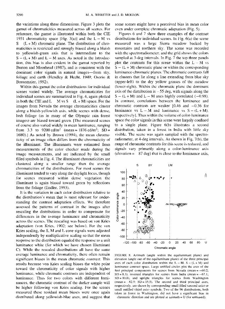
FIGURE 8. Azimuth (angle within the equiluminant plane) and elevation (angle out of the equiluminant plane) of the three principal axes of each color distribution within the L - M, S - (L + M) and luminance contrast space. Large unfilled circles plot the axes of the first principal components for scenes from Nevada (mean = - 6 0 . 2 ; S D = 8.3), inverted triangles for scenes from India ( m e a n = - 6 7 . 1 ; S D = 10.8), and upright triangles for scenes from Washington ( m e a n = - 8 2 . 9 ; SD= 15.5). The second and third principal axes, respectively, are shown by corresponding small filled (second axis) or small unfilled (third axis) symbols. Two of the 96 distributions, both taken in forest in Washington, did not have a significant bias in

chromatic direction and are plotted at azimuth = U (for unbiased).


(a)

120

90 + ©

~ 60

3O

0 0 3O

( b )

120

9O u)

~" 60

30

120

90 (O o ~, 60 r-

E

- 30

I I I

60 90 120

L-M

120

9O 0 ~

< 60 o

• 120 © © -,~

~ 9o

ID 0 g 6o ¢-

I -- 30

o ~ ~ o • 30 ~ 2 ~ ° ° ° •

j o 4 ~ p , , 0 30 60 90 120 0

I I I 1 0

30 60 90 120

L-M

OA

O 0

o

9~oI o %°o

0

I I I I

30 60 90 120

S-(L+M)

120

9O (/)

6o

3O

0 I ~ ( 5 ' • 0 0 J ' ' 0 30 60 90 120 0 30 60 90 120

Axis 1 Axis 1 Axis 2

FIGURE 9. RMS Contrasts for individual scenes. In (a), each panel plots the RMS contrasts along different pairs of cardinal axes. ©, Distributions from Nevada; O, distributions from India; and A, for distributions from Washington. The average RMS contrast was 59.8 (luminance), 36.9 [S - (L + M)] and 22.3 (L - M). In (b), the RMS contrasts are replotted in terms of the principal axes for each distribution. The

average contrast across scenes was 74.0 (first axis), 25.3 (second axis) and 8.1 (third axis).

and a chromatic axis ( - 9 3 deg) very close to the S - (L + M) axis. Consequently there is little correlation (< 0.10) between signals along any pair of cardinal axes. Finally, Fig. 6(c) shows a scene reconstructed from the digital camera images (of meadow and pines from close range) that exhibits a still more restricted gamut. Chro- matic signals cluster along an axis of - 6 2 deg ( r= -0 .68) and luminance and chromatic contrasts are in this case highly correlated [0.76 for luminance vs L - M contrast; - 0 . 7 6 for luminance vs S - (L + M) contrast]. Individual scenes thus showed marked differences in contrast and in the axes along which the color signals vary.

We estimated for each distribution the three principal axes along which the color signals varied (following von Kries scaling). The axes are plotted in Fig. 8 in terms of their angle within the L - M vs S - (L + M) chromatic plane and elevation out of the equiluminant plane. The dominant axes vary widely in elevation, but are confined to a range of chromatic angles between - 9 9 and - 4 3 deg. The second principal axis usually had a chromatic angle similar to the dominant axis (and thus an elevation roughly 90 deg from the dominant axis), while the third component was always close to the equiluminant axis but 90 deg from the chromatic angle of the dominant axis. This indicates that the distributions

tended to be oriented along planes perpendicular to the equiluminant plane, though individual scenes varied widely in their bias (from scenes in which color variations were confined almost to a single axis to two scenes without a measurable bias in color direction).

While the range of chromatic angles is substantial, it nevertheless represents only a modest fraction of the full 180-deg range of possible axes, and is roughly delimited by two axes that have been emphasized in alternative models of post-receptoral color processing: the S - (L+ M) cardinal axis (4-90 deg) and an axis of perceptually pure blue-yellow variation that is central to models of color appearance [roughly - 5 5 deg; Hurvich and Jameson (1957)]. [The angle of the blue-yellow axis is an approximation based on our own measurements (Webster & Mollon, 1994, 1997), but can vary substantially depending on observers and viewing conditions.] Blue-yellow variations were more typical of arid scenes while biases along the S - (L+ M) axis were more characteristic of scenes with lush vegetation and little sky. (The latter were also characterized by weaker biases in chromatic contrast.) Most all of the sampled scenes fall in between these extremes and are characterized by high correlations between the two chromatic dimensions, whereas correlations between luminance and chromatic

3292 M . A . W E B S T E R and J. D. M O L L O N

(a)

100

~- 50 + _J

i

-50

- 1 0 0 I

-100

(b)

100

~- 50 + J " U

o~ 0

-50

-100 i

-100

6000

C~

,•4000 © ° ~ =°

" .~

~2000

I I I I 0 t

-50 0 50 100 -100

L-M

,,_,100

o © E o 50

% o

E .. ~ 0 ) .E

• E

~ ~ -50

i i i i - 1 0 0 i

-50 0 50 100 -100

L-M

6000

;. _J 2000

O I i I I 0

-50 0 50 100 -100

L-M

.,..,100

50

© E ~ 0 .E

-- -50 O

P I

-50 0 50

L-M

O

" ~ ~''40z~..~

0

-50 0 50

S-(L+M)

9

O

O

k.

i - 1 0 0 i i i

100 -100 -50 0 50

S-(L+M)

I

100

k Q

i

100

(c) 3

4- ,,_1 v 0 i O9

-1

-2

3 3

f o 1 O

o 0 t-

.E_ E -1 : 3

...J

-2

I i I I I I I -3 -1 0 1 2 3 -3

L-M

9

o 0 E

t-

F= -I 3

O -J -2

I°i O

0 o

O -3 , i i i i i i -3 , i i i i i J

-3 -2 -2 -I 0 I 2 3 -3 -2 -I 0 I 2 3

L-M S-(L+M)

FIGURE 10. Adaptation to the color distribution of Fig. 7(a), simulated by von Kries scaling followed by decorrelation. (a) The measured chromaticities and luminances for the distribution. The solid circle of filled triangles plot the coordinates of test stimuli that fall on a sphere (of radius = 17) centered on the distribution mean, which has a yellow bias. In (b), yon Kries adaptation rescales the cone signals so that the distribution mean is centered on the unit- luminance white. This causes an equivalent shift in the appearance of the test colors (with the solid circle now representing the shifted test coordinates). (c) The distribution following decorrelation and normalization to unit variance• The sphere of test

stimuli are distorted into an ellipsoid oriented perpendicular to the blue-yel low principal axis of the distribution.

contrast are in most cases weaker but often substantial. If many natural scenes produce correlated responses in the S - (L + M) and L - M channels, then this raises the question of w h y - - o r in what specific environments (e.g. lush foliage)--the visual system evolved to represent colors in terms of these axes.

Figure 9 summarizes the range of contrasts for the scenes we sampled. The three panels in Fig. 9(a) plot for each distribution the RMS contrast along each pair of

cardinal axes. As illustrated above, contrast varies widely across individual scenes. For the two chromatic axes, the contrasts are strongly correlated, consistent with the fact that the color signals in many of the scenes vary along a restricted range of chromatic axes intermediate to the L - M and S - (L + M) axes. The relationships between luminance and chromatic contrast are more variable and exhibit weak negative correlations. These appear to partly reflect a difference between close-up scenes of

ADAPTION AND THE COLOR STATISTICS OF N A T U R A L IMAGES 3293

(a)

10

-5

-20 (,0

-35

-50

-40

(b)

10

-5

+ -20 i

O9

-35

-50

-40

(c)

10

-5

-20 09

-35

-50 .

40 40

,' ~ ', "~ '~ ~ 20

' O o

' ~ " 8 o ¢ =

:, -2o

I I , I I -40 -20 0 20 40 -40

L-M

40

, ' ~ ~ , ' ~ i ~ m 20 4

E

.~_

~ -20

(11 20

' 8 0

3 -20

I I I I t

-20 0 20 40

L-M

I i I i I I - 4 0 i I I i I

-20 0 20 40 -40 -20 0 20

L-M L-M

40

-40

.,~ 20 o L)

.c_ E ~ -2o

-20 0 20

L-M

40

t~ 20 t -

O c)

E

E 3 -2o

I i I I i I t I t

-50 -35 -20 -5 10

S-(L+M)

X'

I - 4 0 I i I i I i I I i

40 -50 -35 -20 -5 10

S-(L+M)

40

20

E ~, -2o

I - 4 0 , ~ I , = J - 4 0 I , I I , I , 4

-40 40 -40 -20 0 20 40 -50 -35 -20 -5 10

L-M S-(L+M)

FIGURE 11. Matches to test stimuli following adaptation to the color distributions of Figure 7. Each panel plots the matches ( Q ) to a set of test stimuli ((3) chosen to span the distribution mean within the three planes defined by pairs of cardinal axes. A , Matches predicted by rescaling the cone signals by von Kries adaptation in order to coincide with the observed match to the mean of the distribution (which is nearly equivalent to the average of the set of test stimuli). (a) Matches following adaptation to the high contrast blue-yel low distribution of Figure 7(a). The matches reveal large losses in perceived contrast that are selective for the blue-yel low chromatic axis while nonselective within either luminance- chromatic plane. (b) Matches after adapting to the distribution of Figure 7(b) show moderate contrast losses selective for the luminance and S - (L + M) axes, consistent with the properties of the adapting distribution. (c) Matches to the low contrast distribution of Figure 7(c) show only

weak losses in perceived contrast but exhibit weak selectivity for the principal axes of the distribution. The observer was MW.

dense vegetation in dappled lighting (which have restricted color gamuts but high luminance-contrast) and panoramic scenes of open areas (which have less pronounced shadows but high color-contrast between the sky and terrain).

The average luminance contrast was 59.8 (unscaled RMS contrast = 0.85) which is similar to the (unscaled)

RMS contrast of 1 reported by van Hateren and van der Schaaf (1996). Nagle and Osorio (1993) found that the spectral placement of the L and M cones minimizes the L - M contrast in natural scenes (compared to hypothe- tical cone pairs with shifted 2max but with the same separation between peaks). For our scaling of the axes the average contrasts in the images are higher for luminance


(a)

10

-5

-20 09

-35

-50

-40 I I

-20

40

~: . % ~ 2 0 ~ .__~-8 0

E =, -20

I , I i I -40

0 20 40 -40

L-M

I I

-20

40

"~ 20

8 o E

3 -20

I t , i - 4 0 I I i J , r

0 20 40 -50 -35 -20 -5 I0 L-M S-(L+M)

(b)

10

-5

+ -J -20 v

i

-35

-50

-40

40

~ 20

4 O

-Z~ E

E 3 -2o

I

-20

40

20

x ~ ~8= o

3 -20

i ~ i i ~ 0 , i i , i i -40 0 20 40 ~0 -20 0 20 40

L-M L-M

I I I t I I I

-50 -35 -20 -5 10

S-(L+M)

(c)

10

-5

+ -20 i

09

-35

40

20 t - O

0 E

E

_~ -20

40

20 t -

.__. E ~ -20

-50 i , i i - 4 0 , i ~ , i , J - 4 0 i , i i , l

-40 -20 0 20 40 -40 -20 0 20 40 -50 -35 -20 -5 I0 L-M L-M S-(L+M)

FIGURE 12. Matches for observer VR for the same conditions as Figure 11. The contrast adaptation effects are similar for both observers, and again reflect the differences between the three adapting distributions. For VR the matches to the test at the mean luminance and chromaticity of the distribution suggest stronger light adaptation than the matches to the test stimuli spanning the mean (perhaps because the former was the only test that does not provide a transient color/luminance change during the test interval). The von Kries predictions shown are based on the average of

the test coordinates.

than color, and higher for S - (L + M) than for L - M chromatic contrasts. However, when scaled by sensitivity to the axes, the differences are not pronounced [roughly in the ratios of 2.7:1.65:1 for luminance: S - ( L + M ) : L - M]. This comparison depends on our specific contrast metric, but suggests that for the low spatial and temporal frequencies at which the scaling is appropriate, relative sensitivity to the different cardinal directions is

reasonably matched to the relative contrasts along those axes in the ensemble of images. [The ratio of luminance to chromatic contrast could be very different if we chose a different scaling, e.g. based on sensitivities to high spatial or temporal frequencies, or based on cone contrasts.]

In Fig. 9(b), a further illustration of the biases in the distributions is given by replotting the image contrasts


along the principal axes that define each distribution (i.e. along the color-luminance axes indicated for individual distributions in Fig. 8). The variance is substantially greater along the principal axis, with little residual contrast along the third axis. Again this indicates that the distributions tend to be restricted to planes within color- luminance space and that some distributions are nearly confined to a single axis.

The color distributions could in principle vary markedly depending on the spatial scale of the measurements. To assess this we examined the distributions based on the camera images after averaging between 1 and 60 x 60 pixels per sample (corresponding to areas of 1 arc min 2 to 1 deg2). Averaging over larger areas usually led to small increases in the correlations between the cardinal axes but had little effect on the principal axes of the distributions. This is illustrated for the distribution in Fig. 7(c), in which unfilled symbols plot the individual pixel values while filled areas plot the values for the samples arranged over 1 deg 2. We also compared the amplitude spectra of the luminance and chromatic images [see also Brelstaff and Troscianko (1992); Derrico & Buchsbaum (1991); Troscianko, P~irraga, Brelstaff, Carr and Nelson (1996)]. For luminance contrast the amplitude spectra of natural images have a characteristic form, decreasing with frequency as 1/f (Burton & Moorhead, 1987; Dong & Atick, 1995; Field, 1987; Ruderman, 1994; Tolhurst, Tadmor & Chao, 1992; van der Schaaf & van Hateren, 1996; Webster & Miyahara, 1997). Con- sistent with these previous studies, the mean slope (c~ = log amplitude/log frequency) for the nine luminance images was - 1 . 12 (SD = 0.11). For the chromatic images the slopes were -0 .88 (SD=0.15) and -1 .01 (SD= 0.17) for the L - M and S - (L + M) axes, respectively. These values are again near - 1 but are slightly yet consistently shallower than the slopes for the luminance spectra. However, we cannot rule out as a basis for this difference a lower signal-to-noise ratio in the chromatic images (which had lower contrast than the luminance images).

Adaptat ion

In order to illustrate how adaptation to the set of colors in a scene might alter color appearance, we modeled adaptation to the color distributions with two stages: an initial stage of light adaptation based on von Kries scaling, followed by a stage of contrast adaptation simulated by decorrelation (Atick et al., 1993; Webster & Mollon, 1995). The theoretical color changes induced by these two stages are shown in Fig. 10 for the distribution of Fig. 7(a). The top panels plot the actual chromaticities and luminances recorded for the image. Within each panel the circle of filled triangles shows a set of stimuli (of contrast = 17) centered on the distribution mean. These represent the coordinates of the test stimuli we used to measure the adaptation effects for this distribution [see Figs. 1 l(a) and 12(a)]. For this scene the average luminance was 2480cd/m 2 and the mean chromaticity was biased toward yellow [L - M = 21.3,

S - (L + M) = -19 .9 ; CIE x, y = 0.340, 0.339]. As noted above, in von Kries scaling the visual system adjusts to the mean luminance and chromaticity of the stimulus by compensatory adjustments in the sensitivity of each cone class, so that the average response for each cone type equals the response to a neutral white. This produces a mean shift in the appearance of all stimuli so that the distribution (and the set of test stimuli) appears centered at the reference white [Fig. 10(b)]. [For this illustration we assume that light adaptation affects only the mean color and not the contrasts. However, rapid light adaptation to individual samples could also alter the effective cone contrasts in response to the scene; see van Hateren and van der Schaaf (1996)].

Contrast adaptation was modeled by adjusting the gain of the von Kries-scaled contrasts along the principal axes of the distributions so that there was equal (unit) variance along each axis. This is equivalent to the decorrelation algorithm of Atick et al. (1993), and results in losses in perceived contrast that are selective for the dominant axes of the distributions. The selectivity of the aftereffects is also predicted by selective adaptation of multiple color-luminance channels, and our adaptation results do not discriminate between these alternatives (Webster & Mollon, 1991, 1994). We use decorrelation because it is computationally convenient and because it has well defined theoretical implications. Figure 10(c) illustrates how decorrelation transforms the von Kries- scaled distribution of Fig. 10(b). Decorrelating the signals induces a relative loss in sensitivity that is strongly selective for the blue-yellow axis of the distribution. This distorts the sphere of contrasts shown in cross section in the three panels of Fig. 10(b) into an ellipsoid oriented at right angles to the dominant axis of the color distribution. The qualitative predictions for contrast adaptation are thus losses in perceived saturation that are selective for the principal axes of the distribution and that vary in magnitude according to the distribution range. However, the model does not provide a quantitative account of contrast adaptation effects, because the multiplicative scaling assumed by the model is not observed in actual measurements of contrast adaptation, which instead exhibit proportionately weaker effects at higher test contrasts (Blakemore et al., 1971; Georgeson, 1985; Webster & Mollon, 1994; Webster, 1996).

Figures 11 and 12 show for two observers the actual color changes produced by adaptation to the distributions illustrated in Fig. 7. The three distributions were chosen as representative of the range of our sample, and differ in their mean chromaticity, contrasts and principal axes. The matches illustrate how adaptation adjusts for each of these properties, in qualitative agreement with the model. Light adaptation (to the distribution mean) shifts the mean perceived color to near-white, and produces corresponding shifts in the test colors. The matches predicted for light adaptation alone are shown by the unfilled triangles, which plot the coordinates for the tests rescaled by von Kries adaptation. Contrast adaptation produces losses in perceived contrast that adjust partially

(a) (b) 20 20

10 10

+,o v i CO

-10

+,o CO

~ ts

i I I i I I

-10 0 10

L-M

-10

I I I I I i

-10 0 10

L-M

-20 i -20 -20 20 -20

3296 M. A, WEBSTER and J. D. MOLLON

I

2O

0.8

oq

"~ 0.6 .,..,

E

:~ 0.4 ¢/) c 0J

CO

(c) (d) 1.0 1.0

0.2

L-M equal variance 2,.::.Al:. ~o~ ~ u "; ~ 0.8

o~

S-(L÷M) ~ O.6

• ~ 0.4 E G)

O9

0.2

5 \equal variance

o??-,

0 . 0 I t I , I I I I I 0 . 0 I I I ~ I i I

0.0 0.5 1.0 1.5 2.0 0.0 0.5 1.0 1.5 2.0

Adaptation Bias (L-M) / S Adaptation Bias (45 deg / 135 deg)

FIGURE 13. Adaptation to biased distributions of chromatic contrast. In (a), adaptation was to a fixed modulation along the S - (L + M) axis (contrast = 48), paired with a variable modulation along the L - M axis (contrast from 0 to 96). The seven sets of points plot the matches to the eight test stimuli ( 0 ) following adaptation to each of the seven adapting ellipses, with the L - M contrast indicated by the number on each curve. (b) Similar results for adapting ellipses that had a fixed contrast along the 135-315 deg axis and variable contrast along the 45-225 deg axis. The observer was MW. (c and d) Estimates of the sensitivity changes along the L - M and S - (L + M) or 135-315 and 45-225 deg axes for two observers. The estimates were based on independent fits of multiplicative sensitivity changes along each axis of the pair. The solid line plots the

sensitivity to the variable axis required to maintain equal perceived contrast for the two axes of the adapting ellipse.

for the d i f f e r en t con t ras t r anges and fo r the p r inc ipa l axes

o f e a c h d is t r ibut ion . Thus , fo r e x a m p l e , adap ta t ion to the

h i g h con t ras t b l u e - y e l l o w va r i a t ion o f the d i s t r ibu t ion in

Fig . 7(a) resul t s in a p r o n o u n c e d loss in p e r c e i v e d co lo r

con t ras t that is s t rong ly s e l e c t i v e for the b l u e - y e l l o w axis

[Figs. l l ( a ) and 12(a)], w h i l e adap ta t ion to the l o w e r -

con t ras t va r i a t ions a long the S - (L + M ) axis o f the

d i s t r ibu t ion in Fig . 7(b) resul t s in w e a k e r con t ras t losses

that are ins tead b i a sed a long the S - (L + M ) axis [Figs.

11 (b) and 12(b)].

T h e ad jus tmen t s to the con t ras t r ange o f i nd iv idua l

d i s t r ibu t ions r ep re sen t a par t ia l t e n d e n c y for the v i sua l

s y s t e m to m a t c h the p r e v a i l i n g g a m u t o f co lo r s ignals and

thus to exh ib i t " con t r a s t c o n s t a n c y " ( B r o w n & M a c L e o d ,


1991). However, the contrast adaptation does not serve to maintain "color constancy" (i.e. a stable representation of object color), for the adaptation will bias the perceived color of an object in different ways depending on the collection of objects in the scene. Similarly, Webster and Mollon (1995) have shown that changes in the illumina- tion on a scene can alter the distribution of color signals and thus induce a change in the state of contrast adaptation. Contrast adaptation may thus play a role in how colors are perceived under different illuminants, but cannot serve to completely discount the illuminant, because the adaptation cannot compensate for the changes in the color directions of distributions induced by an illuminant change. Instead, the selectivity of the contrast adaptation causes perceived color to be biased toward axes orthogonal to the principal axes of the adapting distribution, which correspond to the more novel color directions in a given scene. This could serve both to enhance the perceptual salience of less frequent color signals (Barlow, 1990) and to allow the colors within individual scenes to be encoded more efficiently (Barlow, 1989; Atick et al., 1993), though the magnitude of the aftereffects is substantially weaker than the complete decorrelation predicted by the model.

As noted in Methods, the adaptation effects observed in Figs. 11 and 12 were induced by viewing a rapid succession of colors presented in a uniform field. This simulates for a single retinal locus the pattern of stimulation that might arise from rapid and random eye movements across the image, but does not allow us to assess how the spatial structure of the images might influence the adaptation. Webster and Miyahara (1997) have measured the changes in spatial contrast sensitivity that result from adaptation to gray-level images of scenes. The low-frequency bias in the amplitude spectra of natural images produces selective losses in sensitivity at low spatial frequencies. Because chromatic contrast in scenes also exhibits a low-frequency bias (Brelstaff & Troscianko, 1992; Troscianko et al., 1996; present study), we similarly expect the chromatic contrast adaptation effects to be larger with increasing spatial scale. [The actual changes in spatial sensitivity should depend on both the specific amplitude spectra of the scenes, which may differ for luminance and chromatic contrast, and the contrast sensitivity function, which is very different for luminance and color (Mullen, 1985). We are currently exploring this question.]

The results of Figs. 11 and 12 suggest that the visual system does adjust selectively to the specific color distribution of individual scenes. As a final question, we asked how biased the distribution must be in order to induce a bias in color appearance. For these measurements we used theoretically defined adapting stimuli that were chosen to vary systematically the bias along different chromatic directions. The stimuli were com- posed of 1 Hz sinusoidal modulations along pairs of orthogonal axes within the chromatic plane. Along one axis [the S - ( L + M ) or the 135-315 deg axis] the contrast was fixed at 48, while along the second axis (the

L - M or 45-225 deg axis) contrast was varied on different runs between 0 and 96. The two modulations were combined 90 deg out of phase so that the resulting stimulus varied along an ellipse within the equiluminant plane. Figure 13 shows the matches to a set of eight chromatic test stimuli following adaptation to biases along the cardinal axes [Fig. 13(a)] or the intermediate axes [Fig. 13(b)]. Figures 13(c) and 13(d) show for two observers estimates of the sensitivity changes, calculated from the best-fitting multiplicative sensitivity changes along the two orthogonal axes. Modulations along either fixed-contrast axis produced a constant change in perceived contrast, while losses along the orthogonal axis increased systematically as the adapting contrast along these axes increased. The results suggest that even weak biases in the adapting distribution (e.g. aspect ratios of 0.75 or 1.33) are sufficient to induce color changes that are at least weakly selective for the major axis of the adapting distribution. Again these selective adjustments may tend to offset the contrast biases in the distributions, but do not compensate completely [as shown by the solid lines in Figs. 13(c) and 13(d), which plot the sensitivity changes required for equal perceived contrast along the two adapting axes].

CONCLUSION

Our analysis suggests that the highly restricted color distributions characterizing natural images may provide a potent stimulus for adaptation, inducing strongly selective changes in color appearance. Both the differences and the similarities between the scenes we sampled have important implications. On the one hand, the variability is large enough so that very different contrast adaptation effects will occur for individual scenes, and observers in specific contexts may thus encode colors differently. Similarly, different contrast adaptation effects are likely to arise when the same scene is viewed under different conditions, for example, because of changes in illumina- tion (Webster & Mollon, 1995), the weather (Brown & MacLeod, 1991), or longer term changes in the seasons. On the other hand, our data suggest that natural scenes exhibit a limited range of chromatic distributions, so that the range of adaptation states is normally limited [just as the common spatial structure of natural images may limit the states of spatial contrast adaptation; Webster & Miyahara (1997)]. These must determine the natural operating states of the visual system.

REFERENCES

Atick, J. J., Li, Z. & Redlich, A. N. (1992). Understanding retinal color coding from first principles. Neural Computation, 4, 559-572.

Atick, J. J., Li, Z. & Redlich, A. N. (1993). What does post-adaptation color appearance reveal about cortical color representation? Vision Research, 33, 123-129.

Barlow, H. B. (1990). A theory about the functional role and synaptic mechanism of visual after-effects. In Blakemore, C. (Ed.), Vision: Coding and efficiency. Cambridge: Cambridge University Press.

Barlow, H. B. (1990). Conditions for versatile learning, Helmholtz's unconscious inference, and the task of perception. Vision Research, 30, 1561-1571.


Barlow, H. B. & Ftildi~ik, P. F. (1989). Adaptation and decorrelation in the cortex. In Durbin, R., Miall, C. & Mitchison, G. J. (Eds.), The computing neuron. New York: Addison-Wesley.

Blakemore, C. & Campbell, F. W. (1969). On the existence of neurones in the human visual system selectively sensitive to the orientation and size of retinal images. Journal of Physiology, London, 203, 237-260.

Blakemore, C., Muncey, J. P. J. & Ridley, R. M. (1971). Perceptual fading of a stabilized cortical image. Nature, 233, 204-205.

Bradley, A., Switkes, E. & De Valois, K. K. (1988). Orientation and spatial frequency selectivity of adaptation to color and luminance gratings. Vision Research, 28, 841-856.

Brelstaff, G., P~irraga, A., Troscianko, T. & Carr, D. (1995). Hyper- spectral camera system: Aquisition and analysis. SPIE, 2587, 150- 159.

Brelstaff, G. & Troscianko, T. (1992). Information content of natural scenes: Implications for neural coding of colour and luminance. SP1E Proceedings, 1666, 302-305.

Brown, R. O. (1994). The world is not grey. Investigative Ophthalmology and Visual Science, 35 Suppl., 2165.

Brown, R. O. & MacLeod, D. 1. A. (1991). Induction and constancy for color saturation and achromatic contrast variance. Investigative Ophthalmology and Visual Science, 32 Suppl., 1214.

Buchsbaum, G. & Gottschalk, A. (1983). Trichromacy, opponent colours and optimum colour information transmission in the retina. Proceedings of the Royal Society of London, B 220, 89-113.

Burton, G. J. & Moorhead, I. R. (1987). Color and spatial structure in natural scenes. Applied Optics, 26, 157-170.

Derrico, J. B. & Buchsbaum, G. (1991). A computational model of spatiochromatic image coding in early vision. Journal of Visual Communication and Image Representation, 2, 31-38.

Derrington, A. M., Krauskopf, J. & Lennie, P. (1984). Chromatic mechanisms in lateral geniculate nucleus of macaque. Journal of Physiology, 357, 241-265.

Dong, D. W. & Atick, J. J. (1995). Statistics of time-varying images. Network:Computation in Neural Systems, 6, 345-358.

Endler, J. A. (1993). The color of light in forests and its implications. Ecological Monographs, 63, 1-27.

Field, D. J. (1987). Relations between the statistics of natural images and the response properties of cortical cells. Journal of the Optical Society of America, A, 4, 2379-2394.

Georgeson, M. A. (1985). The effect of spatial adaptation on perceived contrast. Spatial Vision, 1, 103-112.

Gibson, J. J. & Radner, M. (1937). Adaptation, after-effect and contrast in the perception of tilted lines. I. Quantitative studies. Journal of Experimental Psychology, 20, 453-467.

van Hateren, J. H. & van der Schaaf, A. (1996). Temporal properties of natural scenes. SPIE, 2657, 139-143.

Hendley, C. D. & Hecht, S. (1949). The colors of natural objects and terrains, and their relation to visual color deficiency. Journal of the Optical Society of America, A, 39, 870-873.

Hurvich, L. M. & Jameson, D. (1957). An opponent-process theory of color vision. Psychological Review, 64, 384-404.

Judd, D. B., MacAdam, D. L. & Wyszecki, G. (1964). Spectral distribution of typical daylight as a function of correlated color temperature. Journal of the Optical Soeie~, of America, 54, 1031- 1040.

Krhler, W. & Wallach, H. (1944). Figural aftereffects: An investiga- tion of visual processes. Proceedings of the American Philosophical Society, 88, 269-357.

Krauskopf, J., Williams, D. R. & Heeley, D. W. (1982). Cardinal directions of color space. Vision Research, 22, 1123-1131.

Krauskopf, J., Williams, D. R., Mandler, M. B. & Brown, A. M. (1986). Higher order color mechanisms. Vision Research, 26, 23-32.

von Kries, J. (1902). Festschrift der Albrecht-Ludwigs-Universit~it (Fribourg, 1902), translated in MacAdam, D. L. (Ed.), Sources of color science. Cambridge: MIT Press (1970).

Krinov, E. L. (1947). Spectral reflectance properties of natural formations. National Research Council of Canada Technical Trans- lation 439.

Lee, H.-C. (1992). A physics-based color encoding model for images

of natural scenes. Proceedings of the Conference on Modern Engineering and Technology, Electro-Optics Session, Taipei, Taiwan, 6-15 December, pp. 25-52.

Lythgoe, J. N. (1979). The ecology of vision. Oxford: Oxford University Press.

MacLeod, D. I. A. & Boynton, R. M. (1979). Chromaticity diagram showing cone excitation by stimuli of equal luminance. Journal of the Optical Society of America, 69, 1183-1186.

Mollon, J. D. (1989). "Tho' she kneel'd in that Place where they grew...". Journal of Experimental Biology, 146, 21-38.

Moorhead, I. R. (1985). Human color vision and natural images. Colour in information technology and visual displays (IERE, London, Publication No. 61), 61, 2l.

Mullen, K. T. (1985). The contrast sensitivity of human colour vision to red-green and blue-yellow chromatic gratings. Journal of Physiology, 359, 381-409.

Ohzawa, I., Sclar, G. & Freeman, R. D. (1985). Contrast gain control in the cat's visual system. Journal of Neurophysiology, 54, 651-667.

Nagle, M. G. & Osorio, D. (1993). The tuning of human photopigments may minimize red-green chromatic signals in natural conditions. Proceedings of the Royal Society of London B, 252, 209-213.

Osorio, D. & Bossomaier, T. R. J. (1992). Human cone-pigment spectral sensitivities and the reflectances of natural surfaces. Biological Cybernetics, 67, 217-222.

Ruderman, D. L. (1994). The statistics of natural images. Network Computation in Neural Systems, 5, 517-548.

van der Schaaf, A. & van Hateren, J. H. (1996). Modelling the power spectra of natural images: Statistics and information. Vision Research, 36, 2759-2770.

Sclar, G., Lennie, P. & DePriest, D. D. (1989). Contrast adaptation in striate cortex of macaque. Vision Research, 29, 747-755.

Shapley, R. M. & Enroth-Cugell, C. (1984). Visual adaptation and retinal gain controls. In Osborne, N. N. &Chader , G. J. (Eds.), Progress in retinal research (Vol. 3, pp. 263-343). Oxford: Pergamon.

Smirnakis, S. M., Berry, M. J., Warland, D. K., Bialek, W. & Meister, M. (1997). Adaptation of retinal processing to image contrast and spatial scale. Nature, 386, 69-73.

Smith, V. C. & Pokorny, J. (1975). Spectral sensitivity of the foveal cone photopigments between 400 and 500 nm. Vision Research, 15, 161-171.

Tolhurst, D.J., Tadmor, Y. & Chao, T. (1992). The amplitude spectra of natural images. Ophthalmic and Physiological Optics, 12, 229- 232.

Troscianko, T., P~raga, C. A., Brelstaff, G., Carr, D. & Nelson, K. (1996). Spatio-chromatic information content of natural scenes. Perception, 25 Suppl., 46-47.

Webster, M. A. (1996). Human colour perception and its adaptation. Network: Computation in Neural Systems, 7, 587~534.

Webster, M. A. & Miyahara, E. (1997). Contrast adaptation and the spatial structure of natural images. Journal of the Optical Socie~ of America, in press.

Webster, M. A. & Mollon, J. D. (1991). Changes in colour appearance following post-receptoral adaptation. Nature, 349, 235 238.

Webster, M. A. & Mollon, J. D. (1994). The influence of contrast adaptation on color appearance. Vision Research, 34, 1993-2020.

Webster, M. A. & Mollon, J. D. (1995). Colour constancy influenced by contrast adaptation. Nature, 373, 694-698.

Webster, M. A. & Mollon, J. D. (1997). Motion minima for different directions in color space. Vision Research, 37, 1479-1498.

Webster, M. A., Wade, A. & Mollon, J. D. (1996). Color in natural images and its implications for visual adaptation. SPIE, 2657, 144- 152.

Wohlgemuth, A. ( 1911 ). On the after-effect of seen movement. British Journal of Psychology Monograph (Suppl. 1).

Acknowledgements We thank V. Raker, A. Wade and J. Wilson for assistance. Supported by EY10834 and the BBSRC.

adaptation and the color statistics of natural...

Documents