Action Schema Networks: Generalised Policies with Deep Learning

Sam Toyer1, Felipe Trevizan1,2, Sylvie Thiebaux1 and Lexing Xie1,31 Research School of Computer Science, Australian National University 2 Data61, CSIRO 3 Data to Decisions CRC

first.last@anu.edu.au

Abstract

In this paper, we introduce the Action Schema Network (AS-Net): a neural network architecture for learning generalisedpolicies for probabilistic planning problems. By mimickingthe relational structure of planning problems, ASNets are ableto adopt a weight sharing scheme which allows the networkto be applied to any problem from a given planning domain.This allows the cost of training the network to be amortisedover all problems in that domain. Further, we propose a train-ing method which balances exploration and supervised train-ing on small problems to produce a policy which remainsrobust when evaluated on larger problems. In experiments,we show that ASNet’s learning capability allows it to signifi-cantly outperform traditional non-learning planners in severalchallenging domains.

1 IntroductionAutomated planning is the task of finding a sequence of ac-tions which will achieve a goal within a user-supplied modelof an environment. Over the past four decades, there hasbeen a wealth of research into the use of machine learn-ing for automated planning (Jimenez et al. 2012), motivatedin part by the belief that these two essential ingredients ofintelligence—planning and learning—ought to strengthenone other (Zimmerman and Kambhampati 2003). Neverthe-less, the dominant paradigm among state-of-the-art classi-cal and probabilistic planners is still based on heuristic statespace search. The domain-independent heuristics used forthis purpose are capable of exploiting common structuresin planning problems, but do not learn from experience.Top planners in both the deterministic and learning tracksof the International Planning Competition often use ma-chine learning to configure portfolios (Vallati et al. 2015),but only a small fraction of planners make meaningful useof learning to produce domain-specific heuristics or controlknowledge (de la Rosa, Celorrio, and Borrajo 2008). Plan-ners which transfer knowledge between problems in a do-main have been similarly underrepresented in the probabilis-tic track of the competition.

In parallel with developments in planning, we’ve seen aresurgence of interest in neural nets, driven largely by theirsuccess at problems like image recognition (Krizhevsky,

Copyright c© 2018, Association for the Advancement of ArtificialIntelligence (www.aaai.org). All rights reserved.

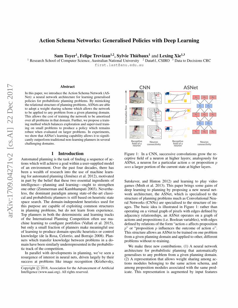
Figure 1: In a CNN, successive convolutions grow the re-ceptive field of a neuron at higher layers; analogously forASNet, a neuron for a particular action a or proposition psees a larger portion of the current state at higher layers.

Sutskever, and Hinton 2012) and learning to play videogames (Mnih et al. 2013). This paper brings some gains ofdeep learning to planning by proposing a new neural net-work architecture, the ASNet, which is specialised to thestructure of planning problems much as Convolutional Neu-ral Networks (CNNs) are specialised to the structure of im-ages. The basic idea is illustrated in Figure 1: rather thanoperating on a virtual graph of pixels with edges defined byadjacency relationships, an ASNet operates on a graph ofactions and propositions (i.e. Boolean variables), with edgesdefined by relations of the form “action a affects propositionp” or “proposition p influences the outcome of action a”.This structure allows an ASNet to be trained on one problemfrom a given planning domain and applied to other, differentproblems without re-training.

We make three new contributions. (1) A neural networkarchitecture for probabilistic planning that automaticallygeneralises to any problem from a given planning domain.(2) A representation that allows weight sharing among ac-tions modules belonging to the same action schema, andamong proposition modules associated with the same pred-icate. This representation is augmented by input features

arX

iv:1

709.

0427

1v2

[cs

.AI]

22

Dec

201

7

from domain-independent planning heuristics. (3) A train-ing method that balances exploration and supervision fromexisting planners. In experiments, we show that this strategyis sufficient to learn effective generalised policies. Code andmodels for this work are available online. 1

2 BackgroundThis work considers probabilistic planning problems repre-sented as Stochastic Shortest Path problems (SSPs) (Bert-sekas and Tsitsiklis 1996). Formally, an SSP is a tuple(S,A, T , C,G, s0) where S is a finite set of states, A is afinite set of actions, T : S × A × S → [0, 1] is a transitionfunction, C : S × A → (0,∞) is a cost function, G ⊆ S isa set of goal states, and s0 is an initial state. At each state s,an agent chooses an action a from a set of enabled actionsA(s) ⊆ A, incurring a cost of C(s, a) and causing it to tran-sition into another state s′ ∈ S with probability T (s, a, s′).

The solution of an SSP is a policy π : A×S → [0, 1] suchthat π(a | s) is the probability that action a will be applied instate s. An optimal policy π∗ is any policy that minimisesthe total expected cost of reaching G from s0. We do not as-sume that the goal is reachable with probability 1 from s0(i.e. we allow problems with unavoidable dead ends), anda fixed-cost penalty is incurred every time a dead end isreached (Mausam and Kolobov 2012).

A factored SSP is a compact representation of an SSP asa tuple (P,A, s0, s?, C). P is a finite set of binary propo-sitions and the state space S is the set of all binary stringsof size |P|. Thus, a state s is a value assignment to all thepropositions p ∈ P . A partial state is a value assignment toa subset of propositions; a partial state s is consistent witha partial state s′ if the value assignments of s′ are containedin s (s′ ⊆ s for short). The goal is represented by a partialstate s?, and G = {s ∈ S|s? ⊆ s}. Each action a ∈ A con-sists in a precondition prea represented by a partial state, aset of effects eff a each represented by a partial state, and aprobability distribution Pra over effects in eff a.2 The ac-tions applicable in state s are A(s) = {a ∈ A | prea ⊆ s}.Moreover, T (s, a, s′) =

∑e∈eff a|s′=res(s,e) Pra(e) where

res(s, e) ∈ S is the result of changing the value of proposi-tions of s to make it consistent with effect e.

A lifted SSP compactly represents a set of factored SSPssharing the same structure. Formally, a lifted SSP is a tu-ple (F ,A, C) where F is a finite set of predicates, andA is a finite set of action schemas. Each predicate, whengrounded, i.e., instantiated by a tuple of names representingobjects, yields a factored SSP proposition. Similarly, eachaction schema, instantiated by a tuple of names, yields a fac-tored SSP action. The Probabilistic Planning Domain Defi-nition Language (PPDDL) is the standard language to de-scribe lifted and factored SSPs (Younes and Littman 2004).PPDDL splits the description into a general domain and aspecific problem. The domain gives the predicates F , action

1https://github.com/qxcv/asnets2 Factored SSPs sometimes support conditional effects and neg-

ative or disjunctive preconditions and goals. We do not use thesehere to simplify notation. However, ASNet can easily be extendedto support these constructs.

schemas A and cost function C specifying a lifted SSP. Theproblem additionally gives the set of objects O, initial states0 and goal s?, describing a specific SSP whose propositionsand actions are obtained by grounding the domain predicatesand action schemas using the objects in O. For instance thedomain description might specify a predicate at(?l) and anaction schema walk(?from, ?to), while the problem descrip-tion might specify objects home and work. Grounding us-ing these objects would produce propositions at(home) andat(work), as well as ground actions walk(work,home) andwalk(home,work).

Observe that different factored SSPs can be obtained bychanging only the problem part of the PPDDL descriptionwhile reusing its domain. In the next section, we show howto take advantage of action schema reuse to learn policiesthat can then be applied to any factored SSP obtained byinstantiating the same domain.

3 Action Schema NetworksNeural networks are expensive to train, so we would like toamortise that cost over many problems by learning a gener-alised policy which can be applied to any problem from agiven domain. ASNet proposes a novel, domain-specialisedstructure that uses the same set of learnt weights θ regard-less of the “shape” of the problem. The use of such a weightsharing scheme is key to ASNet’s ability to generalise todifferent problems drawn from the same domain, even whenthose problems have different goals or different numbers ofactions and propositions.

3.1 Network structureAt a high level, an ASNet is composed of alternating actionlayers and proposition layers, where action layers are com-posed of a single action module for each ground action, andproposition layers likewise are composed of a single propo-sition module for each ground proposition; this choice ofstructure was inspired by the alternating action and propo-sition layers of Graphplan (Blum and Furst 1997). In thesame way that hidden units in one layer of a CNN connectonly to nearby hidden units in the next layer, action modulesin one layer of an ASNet connect only to directly relatedproposition modules in the next layer, and vice versa. Thelast layer of an ASNet is always an action layer with eachmodule defining an action selection probability, thus allow-ing the ASNet to scale to problems with different numbers ofactions. For simplicity, we also assume that the first (input)layer is always an action layer.

Action module details. Consider an action module fora ∈ A in the lth action layer. The module takes as input afeature vector ula, and produces a new hidden representation

φla = f(W la · ula + bla) ,

where W la ∈ Rdh×dla is a learnt weight matrix for the mod-

ule, bla ∈ Rdh is a learnt bias vector, f(·) is a nonlinearity(e.g. tanh, sigmoid, or ReLU), dh is a (fixed) intermediaterepresentation size, and dla is the size of the inputs to theaction module. The feature vector ula, which serves as in-put to the action module, is constructed by enumerating the

propositions p1, p2, . . . , pM which are related to the actiona, and then concatenating their hidden representations. For-mally, we say that a proposition p ∈ P is related to an actiona ∈ A, denoted R(a, p), if p appears in prea or in an effecte where Pra(e) > 0. Concatenation of representations forthe related propositions produces a vector

ula =[ψl−11

T · · · ψl−1M

T]T

,

where ψl−1j is the hidden representation produced by theproposition module for proposition pj ∈ P in the precedingproposition layer. Each of these constituent hidden represen-tations has dimension dh, so ula has dimension dla = dh ·M .

Our notion of propositional relatedness ensures that, ifground actions a1 and a2 in a problem are instances of thesame action schema in a PPDDL domain, then their inputsul1 and ul2 will have the same “structure”. To see why, notethat we can determine which propositions are related to agiven ground action a by retrieving the corresponding ac-tion schema, enumerating the predicates which appear in theprecondition or the effects of the action schema, then instan-tiating those predicates with the same parameters used toinstantiate a. If we apply this procedure to a1 and a2, wewill obtain lists of related propositions p1, p2, . . . , pM andq1, q2, . . . , qM , respectively, where pj and qj are proposi-tions with the same predicate which appear in the same po-sition in the definitions of a1 and a2 (i.e. the same locationin the precondition, or the same position in an effect).

Such structural similarity is key to ASNet’s generalisationabilities. At each layer l, and for each pair of ground actionsc and d instantiated from the same action schema s, we usethe same weight matrix W l

s and bias vector bls—that is, wehave W l

c = W ld = W l

s and blc = bld = bls. Hence, modulesfor actions which appear in the same layer and correspond tothe same action schema will use the same weights, but mod-ules which appear in different layers or which correspondto different schemas will learn different weights. Althoughdifferent problems instantiated from the same PPDDL do-main may have different numbers of ground actions, thoseground actions will still be derived from the same, fixed setof schemas in the domain, so we can apply the same set ofaction module weights to any problem from the domain.

The first and last layers of an ASNet consist of actionmodules, but their construction is subtly different:

1. The output of a module for action a in the final layer isa single number πθ(a | s) representing the probability ofselecting action a in the current state s under the learntpolicy πθ, rather than a vector-valued hidden representa-tion. To guarantee that disabled actions are never selected,and ensure that action probabilities are normalised to 1,we pass these outputs through a masked softmax activa-tion which ensures that πθ(a | s) = 0 if a /∈ A(s). Duringtraining, we sample actions from πθ(a | s). During eval-uation, we select the action with the highest probability.

2. Action modules in the first layer of a ASNet are passed aninput vector composed of features derived from the cur-rent state, rather than hidden representations for relatedpropositions. Specifically, modules in the first layer are

given a binary vector indicating the truth values of relatedpropositions, and whether those propositions appear in thegoal. In practice, it is helpful to concatenate these propo-sitional features with heuristic features, as described inSection 3.2.Proposition module details. Proposition modules only

appear in the intermediate layers of an ASNet, but are oth-erwise similar to action modules. Specifically, a propositionmodule for proposition p ∈ P in the lth proposition layer ofthe network will compute a hidden representation

ψlp = f(W lp · vlp + blp) ,

where vlp is a feature vector, f is the same nonlinearity used

before, and W lp ∈ Rdh×d

lp and blp ∈ Rdh are learnt weights

and biases for the module.To construct the input vlp, we first find the predicate

pred(p) ∈ F for proposition p ∈ P , then enumerate allaction schemas A1, . . . , AL ∈ A which reference pred(p)in a precondition or effect. We can define a feature vector

vlp =

pool({φlaT | op(a) = A1 ∧R(a, p)})

...pool({φla

T | op(a) = AL ∧R(a, p)})

,

where op(a) ∈ A denotes the action schema for ground ac-tion a, and pool is a pooling function that combines severaldh-dimensional feature vectors into a single dh-dimensionalone. Hence, when all pooled vectors are concatenated, thedimensionality dlp of vlp becomes dh · L. In this paper, weassume that pool performs max pooling (i.e. keeps only thelargest input). If a proposition module had to pool over theoutputs of many action modules, such pooling could po-tentially obscure useful information. While the issue couldbe overcome with a more sophisticated pooling mechanism(like neural attention), we did not find that max poolingposed a major problem in the experiments in Section 5, evenon large Probabilistic Blocks World instances where someproposition modules must pool over thousands of inputs.

Pooling operations are essential to ensure that proposi-tion modules corresponding to the same predicate have thesame structure. Unlike action modules corresponding to thesame action schema, proposition modules corresponding tothe same predicate may have a different number of inputsdepending on the initial state and number of objects in aproblem, so it does not suffice to concatenate inputs. As anexample, consider a single-vehicle logistics problem wherethe location of the vehicle is tracked with propositions ofthe form at(ι), and the vehicle may be moved with actionsof the form move(ιfrom, ιto). A location ι1 with one incom-ing road and no outgoing roads will have only one relatedmove action, but a location ι2 with two incoming roads andno outgoing roads will have two related move actions, onefor each road. This problem is not unique to planning: a sim-ilar trick is employed in network architectures for graphswhere vertices can have varying in-degree (Jain et al. 2016;Kearnes et al. 2016).

As with the action modules, we share weights betweenproposition modules for propositions corresponding to the

same predicate. Specifically, at proposition layer l, and forpropositions q and r with pred(q) = pred(r), we tie thecorresponding weights W l

q = W lr and blq = blr. Together

with the weight sharing scheme for action modules, this en-ables us to learn a single set of weights

θ ={W la, b

la | 1 ≤ l ≤ n+ 1, a ∈ A}

∪{W lp, b

lp | 1 ≤ l ≤ n, p ∈ F}

for an n-layer model which can be applied to any problemin a given PPDDL domain.

3.2 Heuristic features for expressivenessOne limitation of the ASNet is the fixed receptive field of thenetwork; in other words, the longest chain of related actionsand propositions which it can reason about. For instance,suppose we have I locations ι1, . . . , ιI arranged in a line inour previous logistics example. The agent can move fromιk−1 to ιk (for k=2, . . . , I) with the move(ιk−1, ιk) action,which makes at(ιk−1) false and at(ιk) true. The proposi-tions at(ι1) and at(ιI) will thus be related only by a chainof move actions of length I−1; hence, a proposition modulein the lth proposition layer will only be affected by at propo-sitions for locations at most l + 1 moves away. Deeper net-works can reason about longer chains of actions, but that anASNet’s (fixed) depth necessarily limits its reasoning powerwhen chains of actions can be arbitrarily long.

We compensate for this receptive field limitation by sup-plying the network with features obtained using domain-independent planning heuristics. In this paper, we derivethese features from disjunctive action landmarks producedby LM-cut (Helmert and Domshlak 2009), but features de-rived from different heuristics could be employed in thesame way. A disjunctive action landmark is a set of actionsin which at least one action must be applied along any opti-mal path to the goal in a deterministic, delete-relaxed versionof the planning problem. These landmarks do not necessarilycapture all useful actions, but in practice we find that provid-ing information about these landmarks is often sufficient tocompensate for network depth limitations.

In this paper, a module for action a in the first networklayer is given a feature vector

u1a =[cT vT gT

]T.

c ∈ {0, 1}3 indicates whether ai is the sole action in at leastone LM-cut landmark (c1 = 1), an action in a landmarkof two or more actions (c2 = 1), or does not appear in alandmark (c3 = 1). v ∈ {0, 1}M represents the M relatedpropositions: vj is 1 iff pj is currently true. g ∈ {0, 1}Mencodes related portions of the goal state, and gj is 1 iff pjis true in the partial state s? defining the goal.

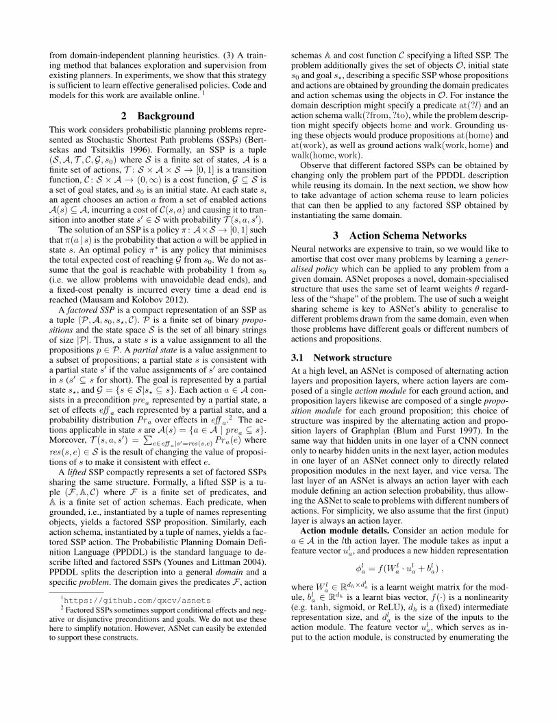
4 Training with exploration and supervisionWe learn the ASNet weights θ by choosing a set of smalltraining problems Ptrain, then alternating between guided ex-ploration to build up a state memory M, and supervisedlearning to ensure that the network chooses good actionsfor the states in M. Algorithm 1 describes a single epoch

Algorithm 1 Updating ASNet weights θ using state memoryM and training problem set Ptrain

1: procedure ASNET-TRAIN-EPOCH(θ,M)2: for i = 1, . . . , Texplore do . Exploration3: for all ζ ∈ Ptrain do4: s0, . . . , sN ← RUN-POL(s0(ζ), π

θ)5: M←M∪ {s0, . . . , sN}6: for j = 0, . . . , N do7: s∗j , . . . , s

∗M ← POL-ENVELOPE(sj , π

∗)8: M←M∪ {s∗j , . . . , s∗M}9: for i = 1, . . . , Ttrain do . Learning

10: B ← SAMPLE-MINIBATCH(M)

11: Update θ using dLθ(B)dθ (Equation 1)

of exploration and supervised learning. We repeatedly ap-ply this procedure until performance on Ptrain ceases to im-prove, or until a fixed time limit is reached. Note that thisstrategy is only intended to learn the weights of an ASNet—module connectivity is not learnt, but rather obtained froma grounded representation using the notion of relatednesswhich we described earlier.

In the exploration phase of each training epoch, we repeat-edly run the ASNet policy πθ from the initial state of eachproblem ζ ∈ Ptrain, collecting N + 1 states s0, . . . , sN vis-ited along each of the sampled trajectories. Each such trajec-tory terminates when it reaches a goal, exceeds a fixed limitL on length, or reaches a dead end. In addition, for eachvisited state sj , we compute an optimal policy π∗ rooted atsj , then produce a set of states s∗j , . . . , s

∗M which constitute

π∗’s policy envelope—that is, the states which π∗ visits withnonzero probability. Both the trajectories drawn from theASNet policy πθ and policy envelopes for the optimal policyπ∗ are added to the state memory M. Saving states whichcan be visited under an optimal policy ensures that M al-ways contains states along promising trajectories reachablefrom s0. On the other hand, saving trajectories from the ex-ploration policy ensures that ASNet will be able to improveon the states which it visits most often, even if they are noton an optimal goal trajectory.

In the training phase, small subsets of the states in Mare repeatedly sampled at random to produce minibatchesfor training ASNet. The objective to be minimised for eachminibatch B is the cross-entropy classification loss

Lθ(B) =∑s∈B

∑a∈A

[(1− ys,a) · log(1− πθ(a | s))

+ ys,a · log πθ(a | s)].

(1)

The label ys,a is 1 if the expected cost of choosing action aand then following an optimal policy thereafter is minimalamong all enabled actions; otherwise, ys,a = 0. This en-courages the network to imitate an optimal policy. For eachsampled batch B, we compute the gradient dLθ(B)dθ and use itto update the weights θ in a direction which decreasesLθ(B)with Adam (Kingma and Ba 2015).

The cost of computing an optimal policy during super-vised learning is often non-trival. It is natural to ask whether

it is more efficient to train ASNets using unguided policygradient reinforcement learning, as FPG does (Buffet andAberdeen 2009). Unfortunately, we found that policy gradi-ent RL was too noisy and inefficient to train deep networkson nontrivial problems; in practice, the cost of computing anoptimal policy for small training problems more than paysfor itself by enabling us to use sample-efficient supervisedlearning instead of reinforcement learning. In the experi-ments, we investigate the question of whether suboptimalpolicies are still sufficient for supervised training of ASNets.

Past work on generalised policy learning has employedlearnt policies as control knowledge for search algorithms,in part because doing so can compensate for flaws in the pol-icy. For example, Yoon, Fern, and Givan (2007) suggest em-ploying policy rollout or limited discrepancy search to avoidthe occasional bad action recommended by a policy. Whilewe could use an ASNet similarly, we are more interested inits ability to learn a reliable policy on its own. Hence, duringevaluation, we always choose the action which maximisesπθ(a | s). As noted above, this is different from the explo-ration process employed during training, where we insteadsample from πθ(a | s).

5 Experiments and discussionIn this section, we compare ASNet against state-of-the-artplanners on three planning domains.

5.1 Experimental setupWe compare ASNet against three heuristic-search-basedprobabilistic planners: LRTDP (Bonet and Geffner 2003),ILAO* (Hansen and Zilberstein 2001) and SSiPP (Trevizanand Veloso 2014). Two domain-independent heuristics areconsidered for each of the three planners—LM-cut (admissi-ble) and the additive heuristic hadd (inadmissible) (Teichteil-Konigsbuch, Vidal, and Infantes 2011)—resulting in 6 base-lines. During evaluation, we enforce a 9000s time cutoff forall the baselines and ASNets, as well as a 10Gb memorycutoff.

Since LRTDP and ILAO* are optimal planners, we exe-cute them until convergence (ε=10−4) for each problem us-ing 30 different random seeds. Notice that, for hadd, LRTDPand ILAO* might converge to a suboptimal solution. If anexecution of LRTDP or ILAO* does not converge before thegiven time/memory cutoff, we consider the planner as hav-ing failed to reach the goal. SSiPP is used as a replanner and,for each problem, it is trained until 60s before the time cut-off and then evaluated; this procedure is repeated 30 timesfor each problem using different random seeds. The train-ing phase of SSiPP consists in simulating a trajectory froms0 and, during this process, SSiPP improves its lower boundon the optimal solution. If 100 consecutive trajectories reachthe goal during training, then SSiPP is evaluated regardlessof the training time left. For the 6 baselines, we report theaverage running time per problem.

For each domain, we train a single ASNet, then evaluateit on each problem 30 times with different random seeds.The hyperparmeters for each ASNet were kept fixed acrossdomains: three action layers and two proposition layers in

each network, a hidden representation size of 16 for each in-ternal action and proposition module, and an ELU (Clevert,Unterthiner, and Hochreiter 2016) as the nonlinearity f . Theoptimiser was configured with a learning rate of 0.0005 anda batch size of 128, and a hard limit of two hours (7200s)was placed on training. We also applied `2 regularisationwith a coefficient of 0.001 on all weights, and dropout onthe outputs of each layer except the last with p = 0.25. Eachepoch of training alternated between 25 rounds of explo-ration shared equally among all training problems, and 300batches of network optimisation (i.e. Texplore = 25/|Ptrain|and Ttrain = 300). Sampled trajectory lengths are L = 300for both training and evaluation. LRTDP with the LM-cutheuristic is used for computing the optimal policies duringtraining, with a dead-end penalty of 500. We also repeatedthis procedure for LRTDP using hadd (inadmissible heuris-tic) to compare the effects of using optimal and suboptimalpolicies for training. Further, we report how well ASNet per-forms when it is guided by hadd, but not given the LM-cut-derived heuristic features described in Section 3.2. For theASNets, we report the average training time plus time tosolve the problem to highlight when it pays off to spend theone-off cost of training an ASNet for a domain.

All ASNets were trained and evaluated on a virtual ma-chine equipped with 62GB of memory and an x86-64 pro-cessor clocked at 2.3GHz. For training and evaluation, eachASNet was restricted to use a single, dedicated processorcore, but resources were otherwise shared. The baselineplanners were run in a cluster of x86-64 processors clockedat 2.6GHz and each planner again used only a single core.

5.2 DomainsWe evaluate ASNets and the baselines on the followingprobabilistic planning domains:

CosaNostra Pizza: as a Deliverator for CosaNostraPizza, your job is to safely transport pizza from a shop toa waiting customer, then return to the shop. There is a se-ries of toll booths between you and the customer: at eachbooth, you can either spend a time step paying the operator,or save a step by driving through without paying. However,if you don’t pay, the (angry) operator will try to drop a boomon your car when you pass through their booth on the wayback to the shop, crushing the car with 50% probability. Theoptimal policy is to pay operators when travelling to the cus-tomer to ensure a safe return, but not pay on the return tripas you will not revisit the booth. Problem size is the numberof toll booths between the shop and the customer. ASNetsare trained on sizes 1-5, and tested on sizes 6+.

Probabilistic Blocks World is an extension of the well-known deterministic blocks world domain in which a roboticarm has to move blocks on a table into a goal configuration.The actions to pick up a block or to put a block on top ofanother fail with probability 0.25; failure causes the targetblock to drop onto the table, meaning that it must be pickedup and placed again. We randomly generate three differentproblems for each number of blocks considered during test-ing. ASNet is trained on five randomly generated problemsof each size from 5–9, for 25 training problems total.

Triangle Tire World (Little and Thiebaux 2007): each

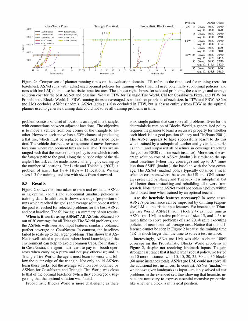
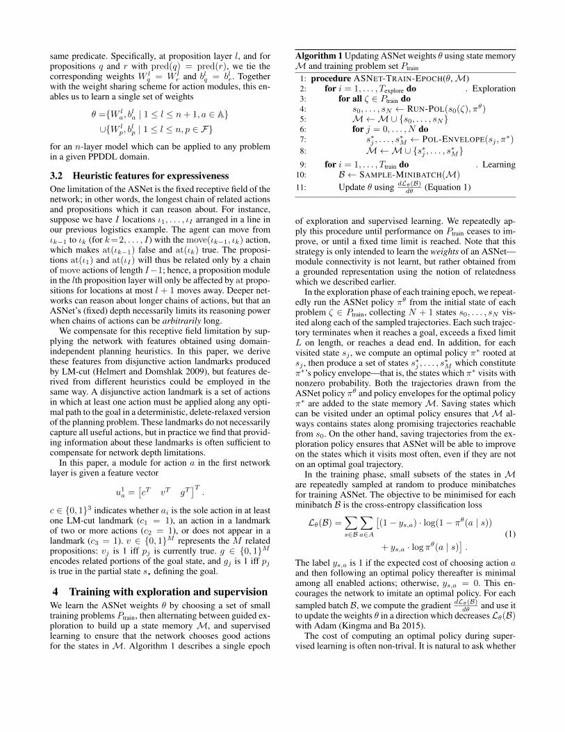
Figure 2: Comparison of planner running times on the evaluation domains. TR refers to the time used for training (zero forbaselines). ASNet runs with (adm.) used optimal policies for training while (inadm.) used potentially suboptimal policies, andruns with (no LM) did not use heuristic input features. The table at right shows, for selected problems, the coverage and averagesolution cost for the best ASNet and baseline. We use TTW for Triangle Tire World, CN for CosaNostra Pizza, and PBW forProbabilistic Blocks World. In PBW, running times are averaged over the three problems of each size. In TTW and PBW, ASNet(no LM) occludes ASNet (inadm.). ASNet (adm.) is also occluded in TTW, but is absent entirely from PBW as the optimalplanner used to generate training data could not solve all training problems in time.

problem consists of a set of locations arranged in a triangle,with connections between adjacent locations. The objectiveis to move a vehicle from one corner of the triangle to an-other. However, each move has a 50% chance of producinga flat tire, which must be replaced at the next visited loca-tion. The vehicle thus requires a sequence of moves betweenlocations where replacement tires are available. Tires are ar-ranged such that the most reliable policy is one which travelsthe longest path to the goal, along the outside edge of the tri-angle. This task can be made more challenging by scaling upthe number of locations. Per Little and Thiebaux (2007), aproblem of size n has (n + 1)(2n + 1) locations. We usesizes 1-3 for training, and test with sizes from 4 onward.

5.3 ResultsFigure 2 shows the time taken to train and evaluate ASNetusing optimal (adm.) and suboptimal (inadm.) policies astraining data. In addition, it shows coverage (proportion ofruns which reached the goal) and average solution cost whenthe goal is reached for selected problems for the best ASNetand best baseline. The following is a summary of our results:

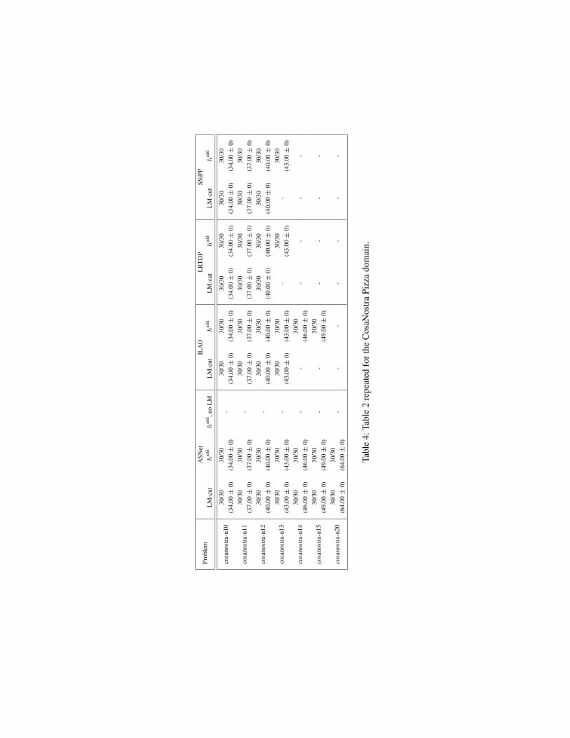
When is it worth using ASNet? All ASNets obtained 30out of 30 coverage for all Triangle Tire World problems, andthe ASNets with heuristic input features similarly obtainedperfect coverage on CosaNostra. In contrast, the baselinesfailed to scale up to the larger problems. This shows that AS-Net is well-suited to problems where local knowledge of theenvironment can help to avoid common traps, for instance:in CosaNostra, the agent must learn to pay toll booth oper-ators when carrying a pizza and not pay otherwise; and inTriangle Tire World, the agent must learn to sense and fol-low the outer edge of the triangle. Not only could ASNetslearn these tricks, but the average solution cost obtained byASNets for CosaNostra and Triangle Tire World was closeto that of the optimal baselines (when they converged), sug-gesting that the optimal solution was found.

Probabilistic Blocks World is more challenging as there

is no single pattern that can solve all problems. Even for thedeterministic version of Blocks World, a generalised policyrequires the planner to learn a recursive property for whethereach block is in a goal position (Slaney and Thiebaux 2001).The ASNet appears to have successfully learnt to do thiswhen trained by a suboptimal teacher and given landmarksas input, and surpassed all baselines in coverage (reachingthe goal on 30/30 runs on each instance). Moreover, the av-erage solution cost of ASNet (inadm.) is similar to the op-timal baselines (when they converge) and up to 3.7 timesless than SSiPP (inadm.), the baseline with the best cover-age. The ASNet (inadm.) policy typically obtained a meansolution cost somewhere between the US and GN1 strate-gies presented by Slaney and Thiebaux: it is suboptimal, butstill better than unstacking and rebuilding all towers fromscratch. Note that the ASNet could not obtain a policy withinthe allotted time when trained by an optimal teacher.

Are the heuristic features necessary? In some cases,ASNet’s performance can be improved by omitting (expen-sive) LM-cut heuristic input features. For instance, in Trian-gle Tire World, ASNet (inadm.) took 2.4x as much time asASNet (no LM) to solve problems of size 15, and 4.3x asmuch time to solve problems of size 20, despite executingpolicies of near-identical average cost. Notice that this dif-ference cannot be seen in Figure 2 because the training time(TR) is much larger than the time to solve a test instance.

Interestingly, ASNet (no LM) was able to obtain 100%coverage on the Probabilistic Blocks World problems inFigure 2, despite not receiving landmark inputs. To gainstronger assurance that it had learnt a robust policy, we testedon 10 more instances with 10, 15, 20, 25, 30 and 35 blocks(60 more instances total). ASNet (no LM) could not solve allthe additional test instances. In contrast, ASNet (inadm.)—which was given landmarks as input—reliably solved all testproblems in the extended set, thus showing that heuristic in-puts are necessary to express essential recursive propertieslike whether a block is in its goal position.

Heuristic inputs also appear to be necessary in CosaNos-tra, where ASNet (no LM) could not achieve full coverageon the test set. We suspect that this is because an ASNetwithout heuristic inputs cannot determine which directionleads to the pizza shop and which direction leads to the cus-tomer when it is in the middle of a long chain of toll booths.

How do suboptimal training policies affect ASNet?Our results suggest that use of a suboptimal policies is suf-ficient to train ASNet, as demonstrated in all three domains.Intuitively, the use of suboptimal policies for training oughtto be beneficial because the time that would have been spentcomputing an optimal policy can instead be used for moreepochs of exploration and supervised learning. This is some-what evident in CosaNostra—where a suboptimal trainingpolicy allows for slightly faster convergence—but it is moreclear in Probabilistic Blocks World, where the ASNet canonly converge within our chosen time limit with the inad-missible policy. While training on fewer problems allowedthe network to converge within the time limit, it did not yieldas robust a policy, suggesting that the use of a suboptimalteacher is sometimes a necessity.

Is ASNet performing fixed-depth lookahead search?No. This can be seen by comparing SSiPP and ASNet.SSiPP solves fixed-depth sub-problems (a generalization oflookahead for SSPs) and is unable to scale up as well as AS-Nets when using an equivalent depth parametrisation. Trian-gle Tire World is particularly interesting because SSiPP canoutperform other baselines by quickly finding dead ends andavoiding them. However, unlike an ASNet, SSiPP is unableto generalize the solution of one sub-problem to the next andneeds to solve all of them from scratch.

6 Related workGeneralised policies are a topic of interest in planning (Zim-merman and Kambhampati 2003; Jimenez et al. 2012; Huand De Giacomo 2011). The earliest work in this area ex-pressed policies as decision lists (Khardon 1999), but thesewere insufficiently expressive to directly capture recursiveproperties, and thus required user-defined support predi-cates. Later planners partially lifted this restriction by ex-pressing learnt rules with concept language or taxonomicsyntax, which can capture such properties directly (Mar-tin and Geffner 2000; Yoon, Fern, and Givan 2002; Yoon,Fern, and Givan 2004). Other work employed features fromdomain-independent heuristics to capture recursive prop-erties (de la Rosa et al. 2011; Yoon, Fern, and Givan2006), just as we do with LM-cut landmarks. Srivastava etal. (2011) have also proposed a substantially different gen-eralised planning strategy that provides strong guaranteeson plan termination and goal attainment, albeit only for arestricted class of deterministic problems. Unlike the de-cision lists (Yoon, Fern, and Givan 2002; Yoon, Fern, andGivan 2004) and relational decision trees (de la Rosa et al.2011) employed in past work, our model’s input features arefixed before training, so we do not fall prey to the rule util-ity problem (Zimmerman and Kambhampati 2003). Further,our model can be trained to minimise any differentiable loss,and could be modified to use policy gradient reinforcementlearning without changing the model. While our approach

cannot give the same theoretical guarantees as Srivastava etal., we are able to handle a more general class of problemswith less domain-specific information.

Neural networks have been used to learn policies for prob-abilistic planning problems. The Factored Policy Gradient(FPG) planner trains a multi-layer perceptron with reinforce-ment learning to solve a factored MDP (Buffet and Aberdeen2009), but it cannot generalise across problems and mustthus be trained anew on each evaluation problem. Concur-rent with this work, Groshev et al. (2017) propose generalis-ing “reactive” policies and heuristics by applying a CNN toa 2D visual representation of the problem, and demonstratean effective learnt heuristic for Sokoban. However, their ap-proach requires the user to define an appropriate visual en-coding of states, whereas ASNets are able to work directlyfrom a PPDDL description.

The integration of planning and neural networks has alsobeen investigated in the context of deep reinforcement learn-ing. For instance, Value Iteration Networks (Tamar et al.2016; Niu et al. 2017) (VINs) learn to formulate and solvea probabilistic planning problem within a larger deep neu-ral network. A VIN’s internal model can allow it to learnmore robust policies than would be possible with ordinaryfeedforward neural networks. In contrast to VINs, ASNetsare intended to learn reactive policies for known planningproblems, and operate on factored problem representationsinstead of (exponentially larger) explicit representations likethose used by VINs.

In a similar vein, Kansky et al. present a model-based RLtechnique known as schema networks (Kansky et al. 2017).A schema network can learn a transition model for an en-vironment which has been decomposed into entities, butwhere those entities’ interactions are initially unknown. Theentity–relation structure of schema networks is reminiscentof the action–proposition structure of an ASNet; however,the relations between ASNet modules are obtained throughgrounding, whereas schema networks learn which entitiesare related from scratch. As with VINs, schema networkstend to yield agents which generalise well across a class ofsimilar environments. However, unlike VINs and ASNets—which both learn policies directly—schema networks onlylearn a model of an environment, and planning on that modelmust be performed separately.

Extension of convolutional networks to other graph struc-tures has received significant attention recently, as such net-works often have helpful invariances (e.g. invariance to theorder in which nodes and edges are given to the network) andfewer parameters to learn than fully connected networks.Applications include reasoning about spatio-temporal rela-tionships between variable numbers of entities (Jain et al.2016), molecular fingerprinting (Kearnes et al. 2016), visualquestion answering (Teney, Liu, and Hengel 2017), and rea-soning about knowledge graphs (Kipf and Welling 2017).To the best of our knowledge, this paper is the first suchtechnique that successfully solves factored representationsof automated planning problems.

7 ConclusionWe have introduced the ASNet, a neural network architec-ture which is able to learn generalised policies for proba-bilistic planning problems. In much the same way that CNNscan generalise to images of arbitrary size by performing onlyrepeated local operations, an ASNet can generalise to dif-ferent problems from the same domain by performing onlyconvolution-like operations on representations of actions orpropositions which are related to one another. In problemswhere some propositions are only related by long chains ofactions, ASNet’s modelling capacity is limited by its depth,but it is possible to avoid this limitation by supplying thenetwork with heuristic input features, thereby allowing thenetwork to solve a range of problems.

While we have only considered supervised learning ofgeneralised policies, the ASNet architecture could in princi-ple be used to learn heuristics or embeddings, or be trainedwith reinforcement learning. ASNet only requires a modelof which actions affect which portion of a state, so it couldalso be used in other settings beyond SSPs, such as MDPswith Imprecise Probabilities (MDPIPs) (White III and El-deib 1994) and MDPs with Set-Valued Transitions (MDP-STs) (Trevizan, Cozman, and Barros 2007). We hope thatfuture work will be able to explore these alternatives anduse ASNets to further enrich planning with the capabilitiesof deep learning.

References[Bertsekas and Tsitsiklis 1996] Bertsekas, D., and Tsitsiklis, J. N.

1996. Neuro-Dynamic Programming. Athena Scientific.[Blum and Furst 1997] Blum, A. L., and Furst, M. L. 1997. Fast

planning through planning graph analysis. AIJ.[Bonet and Geffner 2003] Bonet, B., and Geffner, H. 2003. Labeled

RTDP: improving the convergence of real-time dynamic program-ming. In AAAI.

[Buffet and Aberdeen 2009] Buffet, O., and Aberdeen, D. 2009.The factored policy-gradient planner. AIJ.

[Clevert, Unterthiner, and Hochreiter 2016] Clevert, D.-A.; Un-terthiner, T.; and Hochreiter, S. 2016. Fast and accurate deepnetwork learning by exponential linear units (ELUs). ICLR.

[de la Rosa et al. 2011] de la Rosa, T.; Jimenez, S.; Fuentetaja, R.;and Borrajo, D. 2011. Scaling up heuristic planning with relationaldecision trees. JAIR.

[de la Rosa, Celorrio, and Borrajo 2008] de la Rosa, T.; Celorrio,S. J.; and Borrajo, D. 2008. Learning relational decision treesfor guiding heuristic planning. In ICAPS.

[Groshev et al. 2017] Groshev, E.; Tamar, A.; Srivastava, S.; andAbbeel, P. 2017. Learning generalized reactive policies using deepneural networks. arXiv:1708.07280.

[Hansen and Zilberstein 2001] Hansen, E. A., and Zilberstein, S.2001. LAO: A heuristic search algorithm that finds solutions withloops. Artificial Intelligence.

[Helmert and Domshlak 2009] Helmert, M., and Domshlak, C.2009. Landmarks, critical paths and abstractions: what’s the dif-ference anyway? In ICAPS.

[Hu and De Giacomo 2011] Hu, Y., and De Giacomo, G. 2011.Generalized planning: Synthesizing plans that work for multipleenvironments. In IJCAI.

[Jain et al. 2016] Jain, A.; Zamir, A. R.; Savarese, S.; and Saxena,A. 2016. Structural-RNN: Deep learning on spatio-temporalgraphs. In CVPR.

[Jimenez et al. 2012] Jimenez, S.; de la Rosa, T.; Fernandez, S.;Fernandez, F.; and Borrajo, D. 2012. A review of machine learningfor automated planning. Knowl. Eng. Rev.

[Kansky et al. 2017] Kansky, K.; Silver, T.; Mely, D. A.; Eldawy,M.; Lazaro-Gredilla, M.; Lou, X.; Dorfman, N.; Sidor, S.; Phoenix,S.; and George, D. 2017. Schema networks: Zero-shot transfer witha generative causal model of intuitive physics. In ICML.

[Kearnes et al. 2016] Kearnes, S.; McCloskey, K.; Berndl, M.;Pande, V.; and Riley, P. 2016. Molecular graph convolutions:moving beyond fingerprints. Journal of Computer-Aided Molec-ular Design.

[Khardon 1999] Khardon, R. 1999. Learning action strategies forplanning domains. AIJ.

[Kingma and Ba 2015] Kingma, D., and Ba, J. 2015. Adam: Amethod for stochastic optimization. In ICLR.

[Kipf and Welling 2017] Kipf, T. N., and Welling, M. 2017. Semi-supervised classification with graph convolutional networks. InICLR.

[Krizhevsky, Sutskever, and Hinton 2012] Krizhevsky, A.;Sutskever, I.; and Hinton, G. E. 2012. Imagenet classifica-tion with deep convolutional neural networks. In NIPS.

[Little and Thiebaux 2007] Little, I., and Thiebaux, S. 2007. Prob-abilistic planning vs. replanning. In ICAPS workshops.

[Martin and Geffner 2000] Martin, M., and Geffner, H. 2000.Learning generalized policies in planning using concept languages.In KRR.

[Mausam and Kolobov 2012] Mausam, and Kolobov, A. 2012.Planning with Markov Decision Processes. Morgan & Claypool.

[Mnih et al. 2013] Mnih, V.; Kavukcuoglu, K.; Silver, D.; Graves,A.; Antonoglou, I.; Wierstra, D.; and Riedmiller, M. 2013. PlayingAtari with deep reinforcement learning. In NIPS workshops.

[Niu et al. 2017] Niu, S.; Chen, S.; Guo, H.; Targonski, C.; Smith,M. C.; and Kovacevic, J. 2017. Generalized value iteration net-works: Life beyond lattices. arXiv:1706.02416.

[Slaney and Thiebaux 2001] Slaney, J., and Thiebaux, S. 2001.Blocks world revisited. AIJ.

[Srivastava et al. 2011] Srivastava, S.; Immerman, N.; Zilberstein,S.; and Zhang, T. 2011. Directed search for generalized plansusing classical planners. In ICAPS.

[Tamar et al. 2016] Tamar, A.; Wu, Y.; Thomas, G.; Levine, S.; andAbbeel, P. 2016. Value iteration networks. In NIPS.

[Teichteil-Konigsbuch, Vidal, and Infantes 2011] Teichteil-Konigsbuch, F.; Vidal, V.; and Infantes, G. 2011. ExtendingClassical Planning Heuristics to Probabilistic Planning withDead-Ends. In AAAI.

[Teney, Liu, and Hengel 2017] Teney, D.; Liu, L.; and Hengel, A.v. d. 2017. Graph-structured representations for visual questionanswering. In CVPR.

[Trevizan and Veloso 2014] Trevizan, F., and Veloso, M. 2014.Depth-based Short-sighted Stochastic Shortest Path Problems. Ar-tificial Intelligence.

[Trevizan, Cozman, and Barros 2007] Trevizan, F.; Cozman, F. G.;and Barros, L. N. 2007. Planning under risk and knightian uncer-tainty. In IJCAI.

[Vallati et al. 2015] Vallati, M.; Chrpa, L.; Grzes, M.; McCluskey,T. L.; Roberts, M.; Sanner, S.; et al. 2015. The 2014 InternationalPlanning Competition: Progress and trends. AI Mag.

[White III and Eldeib 1994] White III, C. C., and Eldeib, H. K.1994. Markov decision processes with imprecise transition proba-bilities. Operations Research 42(4):739–749.

[Yoon, Fern, and Givan 2002] Yoon, S.; Fern, A.; and Givan, R.2002. Inductive policy selection for first-order MDPs. In UAI.

[Yoon, Fern, and Givan 2004] Yoon, S.; Fern, A.; and Givan, R.2004. Learning reactive policies for probabilistic planning do-mains. In IPC Probabilistic Track.

[Yoon, Fern, and Givan 2006] Yoon, S. W.; Fern, A.; and Givan, R.2006. Learning heuristic functions from relaxed plans. In ICAPS.

[Yoon, Fern, and Givan 2007] Yoon, S. W.; Fern, A.; and Givan, R.2007. Using learned policies in heuristic-search planning. In IJ-CAI.

[Younes and Littman 2004] Younes, H. L., and Littman, M. L.2004. PPDDL1.0: an extension to PDDL for expressing planningdomains with probabilistic effects.

[Zimmerman and Kambhampati 2003] Zimmerman, T., and Kamb-hampati, S. 2003. Learning-assisted automated planning: lookingback, taking stock, going forward. AI Mag.

A Supplementary material

A.1 Monster experiments

To illustrate when LM-cut flags are not sufficient, we createda simple domain called Monster, in which the agent mustchoose between two n-step paths to reach the goal. This do-main domain uses the same at(ι) predicate and move(ι1, ι2)operators from the running logistics example in the mainpaper. However, at the beginning of each episode, a mon-ster is randomly placed at the final location along one of thetwo paths, and it has a 99% chance of attacking the agent ifthe agent moves to the its location. Since there is still a 1%chance of not attacking the agent, an all-outcome determini-sation cannot indicate which path has the monster on it, andso the agent must look ahead at least n steps to be safe. Oth-erwise, if the agent chooses at random, there is a 50% chancethat they will choose the wrong path, and subsequently hit adead end with high probability.

We perform an experiment on this domain in which wetrain ASNets with increasing depth on problems with pathsfrom length 1-5. We then test on those same problems todetermine what the agent was able to learn. Table 1 showsthe full results. As expected, the only runs with full coverageare those where the ASNet has sufficient depth to see themonster; all others force the ASNet to choose arbitrarily.

Propositionlayers

Path length1 2 3 4 5

1 30/30 14/30 14/30 14/30 14/302 30/30 30/30 14/30 14/30 14/303 30/30 30/30 30/30 14/30 14/304 30/30 30/30 30/30 30/30 14/30

Table 1: Coverage (out of 30) for Monster problem with dif-ferent layer counts.

B Coverage and cost for probabilisticexperiments

To complement the time figures and basic overview of cov-erage given in the main paper, Table 2, Table 3, Table 4 andshow coverage and solution cost for the evaluated proba-bilistic problems.

Prob

lem

ASN

etIL

AO

LR

TD

PSS

iPP

LM

-cut

had

dh

add ,n

oL

ML

M-c

uth

add

LM

-cut

had

dL

M-c

uth

add

tria

ngle

-tir

e-4

30/3

0(2

3.37±

0.66

)30

/30

(23.

37±

0.66

)30

/30

(23.

37±

0.66

)30

/30

(23.

17±

0.69

)30

/30

(23.

17±

0.69

)30

/30

(23.

83±

0.71

)30

/30

(24.

10±

0.76

)30

/30

(23.

23±

0.76

)30

/30

(23.

33±

0.80

)

tria

ngle

-tir

e-5

30/3

0(2

8.87±

0.81

)30

/30

(28.

87±

0.81

)30

/30

(28.

87±

0.81

)-

-30

/30

(29.

27±

0.75

)30

/30

(30.

23±

0.63

)30

/30

(29.

43±

0.85

)30

/30

(29.

83±

0.79

)

tria

ngle

-tir

e-6

30/3

0(3

4.87±

0.94

)30

/30

(34.

87±

0.94

)30

/30

(34.

87±

0.94

)-

--

-30

/30

(35.

70±

0.96

)30

/30

(36.

90±

0.87

)

tria

ngle

-tir

e-7

30/3

0(4

0.77±

0.91

)30

/30

(40.

77±

0.91

)30

/30

(40.

77±

0.91

)-

--

-30

/30

(41.

43±

0.86

)30

/30

(44.

33±

1.05

)

tria

ngle

-tir

e-8

30/3

0(4

6.83±

1.12

)30

/30

(46.

83±

1.12

)30

/30

(46.

83±

1.12

)-

--

-7/

30(4

8.00±

3.66

)26

/30

(50.

77±

1.05

)

tria

ngle

-tir

e-10

30/3

0(5

9.00±

1.11

)30

/30

(59.

00±

1.11

)30

/30

(59.

00±

1.11

)-

--

-1/

30(6

0.00

)-

tria

ngle

-tir

e-9

30/3

0(5

2.93±

1.27

)30

/30

(52.

93±

1.27

)30

/30

(52.

93±

1.27

)-

--

-1/

30(5

4.00

)1/

30(7

1.00

)

tria

ngle

-tir

e-11

30/3

0(6

4.77±

1.08

)30

/30

(64.

77±

1.08

)30

/30

(64.

77±

1.08

)-

--

--

-

tria

ngle

-tir

e-12

30/3

0(7

1.07±

1.21

)30

/30

(71.

07±

1.21

)30

/30

(71.

07±

1.21

)-

--

--

-

tria

ngle

-tir

e-13

30/3

0(7

6.90±

1.21

)30

/30

(76.

90±

1.21

)30

/30

(76.

90±

1.21

)-

--

--

-

tria

ngle

-tir

e-14

30/3

0(8

2.80±

1.35

)30

/30

(82.

80±

1.35

)30

/30

(82.

80±

1.35

)-

--

--

-

tria

ngle

-tir

e-15

30/3

0(8

8.67±

1.37

)30

/30

(88.

67±

1.37

)30

/30

(88.

67±

1.37

)-

--

--

-

tria

ngle

-tir

e-16

30/3

0(9

4.83±

1.29

)30

/30

(94.

83±

1.29

)30

/30

(94.

83±

1.29

)-

--

--

-

tria

ngle

-tir

e-17

30/3

0(1

00.8

0±

1.21

)30

/30

(100

.80±

1.21

)30

/30

(100

.80±

1.21

)-

--

--

-

tria

ngle

-tir

e-18

30/3

0(1

06.5

0±

1.44

)30

/30

(106

.50±

1.44

)30

/30

(106

.50±

1.44

)-

--

--

-

tria

ngle

-tir

e-19

30/3

0(1

12.5

0±

1.56

)30

/30

(112

.50±

1.56

)30

/30

(112

.50±

1.56

)-

--

--

-

tria

ngle

-tir

e-20

30/3

0(1

18.4

3±

1.48

)30

/30

(118

.43±

1.48

)30

/30

(118

.43±

1.48

)-

--

--

-

Tabl

e2:

Cov

erag

e(n

umbe

rofs

ucce

ssfu

ltri

als

tore

ach

the

goal

)for

ase

lect

ion

ofpr

oble

ms

and

plan

ners

.Mea

nco

stto

reac

hth

ego

alan

d95

%C

Ifor

cost

isgi

ven

inbr

acke

ts.

Prob

lem

ASN

etIL

AO

LR

TD

PSS

iPP

LM

-cut

had

dh

add ,n

oL

ML

M-c

uth

add

LM

-cut

had

dL

M-c

uth

add

prob

-bw

-n9-

s1-

30/3

0(2

6.37±

1.60

)30

/30

(26.

37±

1.60

)30

/30

(27.

03±

1.75

)30

/30

(26.

83±

1.83

)3/

30(2

4.67±

3.79

)30

/30

(27.

00±

1.81

)30

/30

(184

.77±

80.7

3)30

/30

(25.

53±

1.58

)

prob

-bw

-n9-

s2-

30/3

0(3

2.57±

1.79

)30

/30

(32.

57±

1.79

)30

/30

(31.

43±

2.21

)30

/30

(32.

67±

2.01

)30

/30

(18.

80±

1.81

)30

/30

(33.

17±

1.70

)13

/30

(480

.08±

147.

47)

30/3

0(3

2.87±

1.91

)

prob

-bw

-n9-

s3-

30/3

0(1

9.27±

1.99

)30

/30

(19.

27±

1.99

)30

/30

(21.

03±

1.78

)30

/30

(21.

67±

2.01

)-

30/3

0(2

0.47±

1.65

)30

/30

(27.

53±

9.11

)30

/30

(20.

33±

1.72

)

prob

-bw

-n10

-s1

-30

/30

(24.

60±

1.97

)30

/30

(24.

60±

1.97

)30

/30

(25.

50±

1.90

)30

/30

(26.

87±

1.71

)-

30/3

0(2

4.03±

1.23

)30

/30

(78.

47±

24.7

6)30

/30

(25.

03±

1.57

)

prob

-bw

-n10

-s2

-30

/30

(33.

87±

2.01

)30

/30

(33.

87±

2.01

)-

30/3

0(3

6.37±

1.96

)-

30/3

0(3

4.27±

1.64

)14

/30

(484

.50±

173.

12)

30/3

0(3

5.27±

1.79

)

prob

-bw

-n10

-s3

-30

/30

(28.

23±

1.96

)30

/30

(28.

73±

2.17

)-

30/3

0(2

9.90±

2.01

)-

30/3

0(2

8.13±

1.77

)30

/30

(127

.20±

33.5

1)30

/30

(28.

60±

1.71

)

prob

-bw

-n15

-s1

-30

/30

(46.

77±

2.52

)30

/30

(49.

23±

2.35

)-

30/3

0(4

8.87±

2.83

)-

30/3

0(5

0.10±

1.92

)30

/30

(94.

23±

10.1

2)30

/30

(51.

27±

1.47

)

prob

-bw

-n15

-s2

-30

/30

(55.

23±

2.31

)30

/30

(55.

50±

2.45

)-

30/3

0(5

7.67±

2.63

)-

30/3

0(5

7.10±

2.49

)30

/30

(185

.00±

33.5

5)30

/30

(58.

60±

2.00

)

prob

-bw

-n15

-s3

-30

/30

(46.

53±

2.60

)30

/30

(48.

50±

2.33

)-

30/3

0(4

6.40±

2.49

)-

30/3

0(4

5.13±

1.83

)30

/30

(249

.20±

50.4

1)30

/30

(46.

00±

2.07

)

prob

-bw

-n20

-s1

-30

/30

(65.

93±

2.39

)30

/30

(70.

33±

2.51

)-

30/3

0(6

9.63±

2.54

)-

30/3

0(7

0.70±

3.36

)-

30/3

0(7

0.00±

2.87

)

prob

-bw

-n20

-s2

-30

/30

(76.

77±

2.11

)30

/30

(76.

77±

2.11

)-

30/3

0(7

3.87±

2.17

)-

30/3

0(7

9.10±

2.73

)-

30/3

0(8

3.53±

3.16

)

prob

-bw

-n20

-s3

-30

/30

(69.

53±

2.81

)30

/30

(77.

30±

2.60

)-

30/3

0(7

4.60±

2.82

)-

30/3

0(7

6.27±

3.44

)-

30/3

0(7

8.20±

3.29

)

prob

-bw

-n25

-s1

-30

/30

(98.

27±

2.99

)30

/30

(99.

47±

2.89

)-

--

17/3

0(1

00.9

4±

4.60

)-

28/3

0(3

23.9

6±

91.4

6)

prob

-bw

-n25

-s2

-30

/30

(91.

50±

2.47

)30

/30

(91.

77±

2.64

)-

--

27/3

0(1

00.7

8±

3.16

)-

30/3

0(1

45.6

3±

27.9

9)

prob

-bw

-n25

-s3

-30

/30

(89.

70±

2.59

)30

/30

(85.

90±

2.00

)-

--

15/3

0(9

5.73±

5.99

)-

29/3

0(1

63.4

1±

35.3

1)

prob

-bw

-n30

-s1

-30

/30

(116

.43±

3.01

)30

/30

(117

.23±

2.77

)-

--

2/30

(107

.50±

44.4

7)-

27/3

0(3

40.3

7±

63.3

1)

prob

-bw

-n30

-s2

-30

/30

(111

.20±

3.36

)30

/30

(113

.27±

3.56

)-

--

--

21/3

0(4

18.3

8±

82.9

5)

prob

-bw

-n30

-s3

-30

/30

(117

.30±

3.33

)30

/30

(119

.00±

2.88

)-

--

--

16/3

0(3

73.3

1±

83.9

3)

prob

-bw

-n35

-s1

-30

/30

(138

.80±

3.37

)30

/30

(138

.87±

3.04

)-

--

--

1/30

(366

.00)

prob

-bw

-n35

-s2

-30

/30

(137

.00±

3.12

)30

/30

(137

.70±

3.41

)-

--

--

3/30

(283

.67±

199.

76)

prob

-bw

-n35

-s3

-30

/30

(139

.27±

3.31

)30

/30

(139

.33±

3.62

)-

--

--

6/30

(287

.33±

137.

80)

Tabl

e3:

Tabl

e2

repe

ated

fort

hePr

obab

ilist

icB

lock

sW

orld

dom

ain.

Prob

lem

ASN

etIL

AO

LR

TD

PSS

iPP

LM

-cut

had

dh

add ,n

oL

ML

M-c

uth

add

LM

-cut

had

dL

M-c

uth

add

cosa

nost

ra-n

1030

/30

(34.

00±

0)30

/30

(34.

00±

0)-

30/3

0(3

4.00±

0)30

/30

(34.

00±

0)30

/30

(34.

00±

0)30

/30

(34.

00±

0)30

/30

(34.

00±

0)30

/30

(34.

00±

0)

cosa

nost

ra-n

1130

/30

(37.

00±

0)30

/30

(37.

00±

0)-

30/3

0(3

7.00±

0)30

/30

(37.

00±

0)30

/30

(37.

00±

0)30

/30

(37.

00±

0)30

/30

(37.

00±

0)30

/30

(37.

00±

0)

cosa

nost

ra-n

1230

/30

(40.

00±

0)30

/30

(40.

00±

0)-

30/3

0(4

0.00±

0)30

/30

(40.

00±

0)30

/30

(40.

00±

0)30

/30

(40.

00±

0)30

/30

(40.

00±

0)30

/30

(40.

00±

0)

cosa

nost

ra-n

1330

/30

(43.

00±

0)30

/30

(43.

00±

0)-

30/3

0(4

3.00±

0)30

/30

(43.

00±

0)-

30/3

0(4

3.00±

0)-

30/3

0(4

3.00±

0)

cosa

nost

ra-n

1430

/30

(46.

00±

0)30

/30

(46.

00±

0)-

-30

/30

(46.

00±

0)-

--

-

cosa

nost

ra-n

1530

/30

(49.

00±

0)30

/30

(49.

00±

0)-

-30

/30

(49.

00±

0)-

--

-

cosa

nost

ra-n

2030

/30

(64.

00±

0)30

/30

(64.

00±

0)-

--

--

--

Tabl

e4:

Tabl

e2

repe

ated

fort

heC

osaN

ostr

aPi

zza

dom

ain.