accurate electromagnetic modeling methods for integrated circuits
TRANSCRIPT
Accurate Electromagnetic Modeling Methods
for Integrated Circuits
Zhifeng Sheng


Accurate Electromagnetic Modeling Methods
for Integrated Circuits
PROEFSCHRIFT
ter verkrijging van de graad van doctor
aan de Technische Universiteit Delft,
op gezag van de Rector Magnificus Prof. ir. K.C.A.M. Luyben,
voorzitter van het College voor Promoties,
in het openbaar te verdedigen op dinsdag 29 juni 2010 om 10.00 uur
door
Zhifeng SHENG
Master of Science in Computer Engineering, Technische Universiteit Delft
geboren te Changsha, Hunan, P. R. China.

ii
Dit proefschrift is goedgekeurd door de promotor:
Prof. dr. ir. P. M. Dewilde
Copromotor:
Dr. ir. R. F. Remis
Samenstelling promotiecommissie:
Rector Magnificus voorzitter
Prof. dr. ir. P. M. Dewilde Technische Universiteit Delft, promotor
Dr. ir. R. F. Remis Technische Universiteit Delft, copromotor
Prof. dr. ir. A. J. van der Veen Technische Universiteit Delft
Prof. dr. S. Chandrasekaran University of California, Santa Barbara
Prof. dr. W. H. A. Schilders Technische Universiteit Eindhoven
Dr. ir. N. P. van der Meijs Technische Universiteit Delft
Dr. W. Schoenmaker Magwel NV
Prof. dr. J. Long Technische Universiteit Delft, reservelid
Copyright c© 2010 by Zhifeng Sheng
All rights reserved. No part of the material protected by this copyright notice may be
reproduced or utilized in any form or by any means, electronic or mechanical, including
photocopying, recording or by any information storage and retrieval system, without the prior
permission of the author.
ISBN: 978-94-6108-053-0
Author email: [email protected]

To my parents and Shanfeng

iv

Contents
List of Figures xi
1 Introduction 1
1.1 Problem Statement and State of the Art . . . . . . . . . . . . . . . . . . . . . . 1
1.2 Content and Contributions of this Dissertation . . . . . . . . . . . . . . . . . . . 5
1.2.1 Surface Integrated Field Equations Method: Chapter 2, 3, 4, 5, 6 . . . . . 5
1.2.2 Hierarchically Semi-separable Theory: Chapter 7 . . . . . . . . . . . . . 6
1.2.3 Multi-Level Hierarchical Schur Algorithm: Chapter 8 . . . . . . . . . . . 7
1.3 Notational Conventions . . . . . . . . . . . . . . . . . . . . . . . . . . . . . . . 8
2 The Electromagnetic Field Equations 11
2.1 Transient Electromagnetic Waves . . . . . . . . . . . . . . . . . . . . . . . . . . 12
2.1.1 The Surface Integrated Field Equations in the Time Domain . . . . . . . 12
2.1.2 The Local Electromagnetic Field Equations . . . . . . . . . . . . . . . . 13
2.1.3 Constitutive Relations . . . . . . . . . . . . . . . . . . . . . . . . . . . 14
2.1.4 Interface Conditions . . . . . . . . . . . . . . . . . . . . . . . . . . . . 14
2.1.5 Initial Condition and Boundary Conditions . . . . . . . . . . . . . . . . 15
2.1.6 Absorbing Boundary Conditions in the Time Domain . . . . . . . . . . . 16
2.2 Maxwell’s Equations in the Frequency Domain . . . . . . . . . . . . . . . . . . 16
2.2.1 The Surface Integrated Field Equations in the Frequency Domain . . . . 16
2.2.2 The Local Electromagnetic Field Equations for Harmonic Waves . . . . . 17
2.2.3 Constitutive Relations . . . . . . . . . . . . . . . . . . . . . . . . . . . 17
2.2.4 Interface Conditions and Boundary Conditions . . . . . . . . . . . . . . 17
2.3 Stationary and Static Field Equations . . . . . . . . . . . . . . . . . . . . . . . . 18
2.3.1 Basic Equations . . . . . . . . . . . . . . . . . . . . . . . . . . . . . . . 18
2.3.2 The Generic Constitutive Relations . . . . . . . . . . . . . . . . . . . . 19
v
vi Contents
2.3.3 Compatibility Relations . . . . . . . . . . . . . . . . . . . . . . . . . . 19
2.3.4 Interface Conditions . . . . . . . . . . . . . . . . . . . . . . . . . . . . 19
2.3.5 Boundary Conditions . . . . . . . . . . . . . . . . . . . . . . . . . . . . 19
2.4 Discussion . . . . . . . . . . . . . . . . . . . . . . . . . . . . . . . . . . . . . . 20
3 Spatial Discretization of the Field Quantities 21
3.1 The Tetrahedron as a Finite Element . . . . . . . . . . . . . . . . . . . . . . . . 21
3.1.1 Basic Symbols on the Triangulation . . . . . . . . . . . . . . . . . . . . 21
3.1.2 Requirements on the Triangulation . . . . . . . . . . . . . . . . . . . . . 22
3.1.3 Geometric Properties of the Tetrahedron . . . . . . . . . . . . . . . . . . 22
3.2 The Linear Expansion Functions . . . . . . . . . . . . . . . . . . . . . . . . . . 26
3.2.1 The Linear Scalar Interpolation Function . . . . . . . . . . . . . . . . . 26
3.2.2 The Linear, Local Expansion Functions . . . . . . . . . . . . . . . . . . 27
3.2.3 The Linear, Nodal Expansion Functions . . . . . . . . . . . . . . . . . . 28
3.2.4 The Linear, Edge Expansion Functions . . . . . . . . . . . . . . . . . . 29
3.2.5 Properties of the Linear, Nodal and Edge Expansion Functions . . . . . . 31
3.2.6 The Linear, Hybrid Expansion Functions . . . . . . . . . . . . . . . . . 32
3.3 Spatial Discretization of Electromagnetic Field Quantities . . . . . . . . . . . . . 34
3.3.1 Spatial Discretization of Field Strengths . . . . . . . . . . . . . . . . . . 34
3.3.2 Material Parameters Expansion . . . . . . . . . . . . . . . . . . . . . . 36
3.3.3 Electromagnetic Fluxes Interpolation . . . . . . . . . . . . . . . . . . . 37
3.3.4 Conduction Current Densities Interpolation . . . . . . . . . . . . . . . . 38
3.3.5 Volume Charge Density Expansion . . . . . . . . . . . . . . . . . . . . 39
3.3.6 Impressed Electric Current Expansion . . . . . . . . . . . . . . . . . . . 39
3.4 Discussion . . . . . . . . . . . . . . . . . . . . . . . . . . . . . . . . . . . . . . 39
4 The Surface Integrated Field Equations Method 41
4.1 Static and Stationary Electric and Magnetic Fields . . . . . . . . . . . . . . . . . 41
4.1.1 Discrete Surface Integrated Curl-Equation . . . . . . . . . . . . . . . . . 41
4.1.2 Discrete Surface Integrated Compatibility Equation . . . . . . . . . . . . 44
4.1.3 Discrete Interface Conditions . . . . . . . . . . . . . . . . . . . . . . . 46
4.1.4 Discrete Boundary Conditions . . . . . . . . . . . . . . . . . . . . . . . 48
4.1.5 Total Number of Equations vs. Total Number of Unknowns . . . . . . . 49
4.1.6 Building the Linear System with the Least-Squares Method . . . . . . . 50
4.1.7 Normalization of the Linear System . . . . . . . . . . . . . . . . . . . . 51
4.2 Electromagnetic Problems in the Frequency Domain . . . . . . . . . . . . . . . 52
4.2.1 Normalization of the Field Quantities . . . . . . . . . . . . . . . . . . . 52
4.2.2 Discrete Ampere’s Equation in the Frequency Domain . . . . . . . . . . 53
4.2.3 Discrete Faraday’s Equation in the Frequency Domain . . . . . . . . . . 56
Contents vii
4.2.4 Discrete Compatibility Equations . . . . . . . . . . . . . . . . . . . . . 56
4.2.5 Discrete Interface Conditions . . . . . . . . . . . . . . . . . . . . . . . 58
4.2.6 Discrete Boundary Conditions . . . . . . . . . . . . . . . . . . . . . . . 59
4.2.7 Total Number of Equations vs. Total Number of Unknowns . . . . . . . 60
4.2.8 Building the Linear System with the Least-Squares Method . . . . . . . 61
4.3 Electromagnetic Problems in the Time Domain . . . . . . . . . . . . . . . . . . 61
4.3.1 Normalization of the Field Quantities . . . . . . . . . . . . . . . . . . . 62
4.3.2 Temporal Discretization Scheme . . . . . . . . . . . . . . . . . . . . . . 62
4.3.3 Discrete Ampere’s Equation in the Time Domain . . . . . . . . . . . . . 62
4.3.4 Discrete Faraday’s Equation in the Time Domain . . . . . . . . . . . . . 65
4.3.5 Discrete Compatibility Equations . . . . . . . . . . . . . . . . . . . . . 66
4.3.6 Discrete Interface Conditions . . . . . . . . . . . . . . . . . . . . . . . 67
4.3.7 Discrete Boundary Conditions . . . . . . . . . . . . . . . . . . . . . . . 68
4.3.8 Total Number of Equations vs. Total Number of Unknowns . . . . . . . 68
4.3.9 Analysis of the Energy Balance . . . . . . . . . . . . . . . . . . . . . . 68
4.3.10 Building the Linear System with the Least-Squares Method . . . . . . . 72
4.3.11 Theoretical Analysis on Computational Complexity . . . . . . . . . . . . 72
4.3.12 Analysis of Over-Determination . . . . . . . . . . . . . . . . . . . . . . 74
4.4 Summary . . . . . . . . . . . . . . . . . . . . . . . . . . . . . . . . . . . . . . 76
5 Electromagnetic Field Computations 79
5.1 Field Computation for Magnetostatic Problems . . . . . . . . . . . . . . . . . . 79
5.1.1 Homogeneous Configuration . . . . . . . . . . . . . . . . . . . . . . . . 79
5.1.2 Configuration with High Contrast . . . . . . . . . . . . . . . . . . . . . 80
5.1.3 Configuration with Extremely High Contrast . . . . . . . . . . . . . . . 82
5.2 Field Computation in the Frequency Domain . . . . . . . . . . . . . . . . . . . 87
5.2.1 Configuration with High Contrast . . . . . . . . . . . . . . . . . . . . . 87
5.2.2 Perfecly Matched Layers in the Frequency Domain . . . . . . . . . . . . 88
5.3 Field Computation in the Time Domain . . . . . . . . . . . . . . . . . . . . . . 88
5.3.1 Homogeneous Configuration . . . . . . . . . . . . . . . . . . . . . . . . 93
5.3.2 Configuration with High Contrast . . . . . . . . . . . . . . . . . . . . . 95
5.3.3 Microstrip Low-Pass Filter Simulated in the Time Domain . . . . . . . . 98
5.3.4 Perfecly Matched Layers in the Time Domain . . . . . . . . . . . . . . . 99
5.4 Discussion . . . . . . . . . . . . . . . . . . . . . . . . . . . . . . . . . . . . . . 100
6 The Implementation of the Software Package 103
6.1 Object-Oriented Design of the Main Classes . . . . . . . . . . . . . . . . . . . . 104
6.1.1 Domain, Mesh . . . . . . . . . . . . . . . . . . . . . . . . . . . . . . . 104
6.1.2 Analysis, Electromagnetic Solvers . . . . . . . . . . . . . . . . . . . . . 108

viii Contents
6.1.3 Initial Field, Boundary Conditions and Source Terms . . . . . . . . . . . 109
6.1.4 KSP Linear Solvers and Preconditioners . . . . . . . . . . . . . . . . . . 109
6.2 Design of the Graphic User Interface . . . . . . . . . . . . . . . . . . . . . . . . 111
6.2.1 Generic Class . . . . . . . . . . . . . . . . . . . . . . . . . . . . . . . . 111
6.2.2 EMmodel and ComputeThread . . . . . . . . . . . . . . . . . . . . . . . 113
6.2.3 EMsolverMainWindow and MeshViewer . . . . . . . . . . . . . . . . . . 113
6.2.4 Snapshot of the Graphic User Interface . . . . . . . . . . . . . . . . . . 115
6.3 Programming Interface of EMsolve3D . . . . . . . . . . . . . . . . . . . . . . . 115
6.4 Discussion on the Implementation . . . . . . . . . . . . . . . . . . . . . . . . . 116
7 Algorithms to Solve Hierarchically Semi-separable Systems 117
7.1 Introduction . . . . . . . . . . . . . . . . . . . . . . . . . . . . . . . . . . . . . 117
7.2 Hierarchical Semi-Separable Systems . . . . . . . . . . . . . . . . . . . . . . . 120
7.3 Matrix Operations Based on HSS Representation . . . . . . . . . . . . . . . . . 123
7.3.1 HSS Addition . . . . . . . . . . . . . . . . . . . . . . . . . . . . . . . . 123
7.3.2 HSS Matrix-Matrix Multiplication . . . . . . . . . . . . . . . . . . . . . 126
7.3.3 HSS Matrix Transpose . . . . . . . . . . . . . . . . . . . . . . . . . . . 128
7.3.4 Generic Inversion Based on the State Space Representation . . . . . . . . 128
7.3.5 LU Decomposition of HSS Matrix . . . . . . . . . . . . . . . . . . . . . 129
7.4 Explicit ULV Factorization . . . . . . . . . . . . . . . . . . . . . . . . . . . . . 138
7.4.1 Treatment of a Leaf . . . . . . . . . . . . . . . . . . . . . . . . . . . . . 139
7.4.2 Merge . . . . . . . . . . . . . . . . . . . . . . . . . . . . . . . . . . . . 141
7.4.3 Formal Algorithm . . . . . . . . . . . . . . . . . . . . . . . . . . . . . 142
7.4.4 Results . . . . . . . . . . . . . . . . . . . . . . . . . . . . . . . . . . . 143
7.4.5 Remarks . . . . . . . . . . . . . . . . . . . . . . . . . . . . . . . . . . 143
7.5 Inverse of Triangular HSS Matrix . . . . . . . . . . . . . . . . . . . . . . . . . 144
7.6 Ancillary Operations . . . . . . . . . . . . . . . . . . . . . . . . . . . . . . . . 147
7.6.1 Column (row) Base Insertion . . . . . . . . . . . . . . . . . . . . . . . . 147
7.6.2 Append a Matrix to a HSS Matrix . . . . . . . . . . . . . . . . . . . . . 149
7.7 Complexity Analysis . . . . . . . . . . . . . . . . . . . . . . . . . . . . . . . . 151
7.8 Connection between SSS, HSS and the Time Varying Notation . . . . . . . . . . 152
7.8.1 From SSS to HSS . . . . . . . . . . . . . . . . . . . . . . . . . . . . . . 152
7.8.2 From HSS to SSS . . . . . . . . . . . . . . . . . . . . . . . . . . . . . . 155
7.9 Design of the HSS Iterative Solver . . . . . . . . . . . . . . . . . . . . . . . . . 157
7.9.1 Preconditioners . . . . . . . . . . . . . . . . . . . . . . . . . . . . . . . 157
7.9.2 Numerical Result . . . . . . . . . . . . . . . . . . . . . . . . . . . . . . 161
7.9.3 Conclusions on Iterative HSS Solvers . . . . . . . . . . . . . . . . . . . 164
7.10 Final Remarks . . . . . . . . . . . . . . . . . . . . . . . . . . . . . . . . . . . . 164

Contents ix
8 3D Capacitance Extraction Based on Multi-Level Hierarchical Schur Algorithm 165
8.1 Introduction to SPACE . . . . . . . . . . . . . . . . . . . . . . . . . . . . . . . 165
8.2 The Hierarchical Schur Algorithm . . . . . . . . . . . . . . . . . . . . . . . . . 167
8.2.1 The Maximum Entropy Inverse . . . . . . . . . . . . . . . . . . . . . . 167
8.2.2 One Level of Hierarchy Up: the ‘Nelis Method’ . . . . . . . . . . . . . . 168
8.3 Limitations of the Algorithms Used in SPACE . . . . . . . . . . . . . . . . . . . 171
8.4 Multi-Level Hierarchical Schur Algorithm . . . . . . . . . . . . . . . . . . . . . 171
8.4.1 Notations . . . . . . . . . . . . . . . . . . . . . . . . . . . . . . . . . . 171
8.4.2 Two Dimensional Scan-window Algorithm . . . . . . . . . . . . . . . . 173
8.4.3 Three Dimensional Scan-window Algorithm . . . . . . . . . . . . . . . 174
8.4.4 Numeric Result . . . . . . . . . . . . . . . . . . . . . . . . . . . . . . . 176
8.4.5 Adaptive Three Dimensional Scan-window Algorithm . . . . . . . . . . 178
8.5 Multi-Level Hierarchical Schur Algorithm Combined with HSS Solver . . . . . . 179
8.5.1 Fast Hierarchically Semi-Separable Solver . . . . . . . . . . . . . . . . 179
8.5.2 The HSS Assisted 2D Scan-window Algorithm . . . . . . . . . . . . . . 182
8.5.3 Reusing the HSS Representation . . . . . . . . . . . . . . . . . . . . . . 184
8.5.4 Analysis of Computational Complexity . . . . . . . . . . . . . . . . . . 184
8.5.5 Limitations of the HSS Assisted 2D Scan-window Algorithm . . . . . . 184
8.6 Complexity of Multi-Level Hierarchical Schur Algorithms . . . . . . . . . . . . 186
8.7 Discussion . . . . . . . . . . . . . . . . . . . . . . . . . . . . . . . . . . . . . . 186
9 Summary and Future Work 187
9.1 Summary . . . . . . . . . . . . . . . . . . . . . . . . . . . . . . . . . . . . . . 187
9.2 Future Work . . . . . . . . . . . . . . . . . . . . . . . . . . . . . . . . . . . . . 190
A The SIFE Method to Solve 2D Time Domain EM Problems 191
A.1 Field Representation . . . . . . . . . . . . . . . . . . . . . . . . . . . . . . . . 191
A.2 2D Discrete Surface Integrated Field Equations . . . . . . . . . . . . . . . . . . 191
A.2.1 Constitutive Relations . . . . . . . . . . . . . . . . . . . . . . . . . . . 193
A.2.2 Discrete Interface Conditions . . . . . . . . . . . . . . . . . . . . . . . 193
A.3 The Linear System and Preconditioned CG-like Method . . . . . . . . . . . . . . 194
A.4 2D High Conductivity Configuration . . . . . . . . . . . . . . . . . . . . . . . . 195
A.5 Discussion . . . . . . . . . . . . . . . . . . . . . . . . . . . . . . . . . . . . . . 196
Bibliography 197
Samenvatting en Toekomstig Werk 205
Acknowledgements 209

x Contents
About the Author 211
List of Figures
1.1 Example of a stack of conductors in a modern VLSI process . . . . . . . . . . . 2
2.1 A surface S in the domain of computation D. ∂S is the boundary of the surface. . 12
2.2 The domain of computation D. . . . . . . . . . . . . . . . . . . . . . . . . . . . 13
3.1 Tetrahedron T (n) and some of its locally defined geometric elements. Here,
(i, j, k, l) is an even permutation of (0, 1, 2, 3), which forms a right-handed system. 23
3.2 Vectorial coordinate of the four nodes, vectorial edges, and vectorial faces delim-
iting the tetrahedron T (n). Here, (i, j, k, l) is an even permutation of (0, 1, 2, 3),
where (0, 1, 2, 3) forms a right-handed system. . . . . . . . . . . . . . . . . . . . 24
3.3 The scalar function Q(x) on the four nodes delimiting the tetrahedron T (n). . . . 30
3.4 The unknown variables of linear, hybrid expansion functions on the tetrahedron
T (n), N (n, l) ∈ NCQ, N (n, j) ∈ N
DQ. Here, (i, j, k, l) is an even permutation of
(0, 1, 2, 3). . . . . . . . . . . . . . . . . . . . . . . . . . . . . . . . . . . . . . . 33
3.5 The unknown variables of linear, hybrid expanded electric field strength on the
tetrahedron T (n), N (n, l) ∈ NCE, N (n, j) ∈ N
DE . Here, (i, j, k, l) is an even
permutation of (0, 1, 2, 3). . . . . . . . . . . . . . . . . . . . . . . . . . . . . . 35
3.6 The unknown variables of linear, hybrid expanded magnetic field strength on the
tetrahedron T (n), N (n, l) ∈ NCH, N (n, j) ∈ N
DH. Here, (i, j, k, l) is an even
permutation of (0, 1, 2, 3). . . . . . . . . . . . . . . . . . . . . . . . . . . . . . 36
4.1 The Curl-equations integrated over the facet F(n, i). . . . . . . . . . . . . . . . 42
4.2 Equation (2.26) applied to the bounding surface of the tetrahedron T (n). . . . . 44
xi

xii List of Figures
4.3 The two tetrahedrons T (n1) and T (n2) share one facet on the interface. We have
n1, n2 ∈ IT and m, u, l ∈ IN . Here, (i1,j1,k1,l1) and (i2,j2,k2,l2) are both even
permutations of (0, 1, 2, 3). For clarity, we pulled the two tetrahedrons a little
bit away from the interface. N (n1, j1), N (u),N (n2, k2), N (n1, k1), N (l),
N (n2, j2) and N (n1, l1),N (m),N (n2, l2), respectively, represent the same
node. . . . . . . . . . . . . . . . . . . . . . . . . . . . . . . . . . . . . . . . . 46
4.4 The two tetrahedra T (n1) and T (n2) share one facet on the interface. We have
n1, n2 ∈ IT , and F2
F(n1,i1)and F2
F(n2,i2)are taken in opposite direction. . . . . . 47
4.5 The two tetrahedrons T (n1) and T (n2) share one facet on the interface. n1, n2 ∈IT . m, u, l ∈ IN . (i1,j1,k1,l1) and (i2,j2,k2,l2) are both even permutations of
(0, 1, 2, 3). For clarity, we pulled the two tetrahedrons a little bit away from the
interface. N (n1, j1), N (u), N (n2, k2), N (n1, k1), N (l), N (n2, j2) and
N (n1, l1),N (m), N (n2, l2) represent, respectively, the same node. . . . . . . 58
5.1 (a): The RMSE(H) computed with the SIFE method and the weighted Galerkin
method versus the total number of finite elements in the mesh. (Base 10 loga-
rithmic x and y axis). (b): The total number of iterations needed by the SIFE
method and the weighted Galerkin method versus the number of finite elements
in the mesh (on a base-10 logarithmic scale. BICGstab method + nest dissection
reordering + ICC(0) are used to solve the system of linear equations). . . . . . . 81
5.2 The magnitude of magnetic field strength. (a): the analytic solution. (b): the
solution computed with weighted Galerkin method based on nodal elements. (c):
the solution computed with the Least-squares integrated field equations method
based on nodal elements. (d): the solution computed with the Least-squares
integrated field equations method based on hybrid elements. . . . . . . . . . . . 83
5.3 (a): The RMSE(H) in the two sub-domains computed with the SIFE method
based on nodal elements, the SIFE based on hybrid elements and the weighted
Galerkin method based on nodal elements versus the number of finite elements
in the mesh. We used base 10 logarithmic x and y axis scales. (b): The number
of iterations needed by the SIFE method based on hybrid elements, the SIFE
method based on nodal elements, and the weighted (w=0.3) Galerkin method
based on nodal elements versus the number of finite elements in the mesh. We
used base 10 logarithmic x and y axis scales. BICGstab method + nest dissection
reordering + ICC(1)/ICC(2) . . . . . . . . . . . . . . . . . . . . . . . . . . . . . 84
5.4 The tetrahedron mesh. The mesh is interface conforming and contains 1973
nodes and 9773 tetrahedrons. The gray area is sub-domain0. The green area is
sub-domain1. . . . . . . . . . . . . . . . . . . . . . . . . . . . . . . . . . . . . 85

List of Figures xiii
5.5 (a): The relative root mean square error inD0 andD1 versus the ratio of contrast.
BICGstab linear iterative solver plus nested dissection reordering and ICC(2) are
used; the accuracy of the linear solver has been set to 1 × 10⁻¹². The SIFE
method based on hybrid elements, the SIFE method based on nodal elements,
and the weighted (w=0.3) Galerkin method based on nodal elements. (b): The
number of iterations needed by iterative linear solvers versus the ratio of contrast;
BICGstab linear iterative solver plus nested dissection reordering and ICC(2)
are used; the accuracy of the iterative linear solver has been set to 1 × 10⁻¹².
The SIFE method based on hybrid elements, the SIFE method based on nodal
elements, and the weighted (w=0.3) Galerkin method based on nodal elements. . 86
5.6 The snapshots of the magnitude of the electric field strength and magnetic field
strength computed with the SIFE method based on hybrid elements. . . . . . . . 89
5.7 Relative mean square error plots for the whole domain of computation and Sub-
domain 1. . . . . . . . . . . . . . . . . . . . . . . . . . . . . . . . . . . . . . . 90
5.8 Relative mean square error plots for Sub-domain 2 and Sub-domain 3. . . . . . . 91
5.9 Relative mean square error plot for Sub-domain 4 and the total number of itera-
tions needed when solving the systems with the CG+SOR method. . . . . . . . . 92
5.10 Plots of the electric and magnetic field strengths in the existence of perfectly
matched layers. . . . . . . . . . . . . . . . . . . . . . . . . . . . . . . . . . . . 93
5.11 The tetrahedron mesh consisting of 16608 nodes and 94759 tetrahedrons. . . . . 94
5.12 RMSE versus time step size; Base 10 logarithmic x and y axis (a). The total
number of iterations needed versus time step size; BICGstab iterative solver and
ICC(0) is used for the least-squares SIFE method, BICGstab iterative solver and
ILU(0) is used for the weighted Galerkin’s method. The accuracy of these itera-
tive solvers is set to be 10−12 (b). . . . . . . . . . . . . . . . . . . . . . . . . . . 96
5.13 BICGstab iterative solver + nest-dissection reordering + ICC(4) is used for the
SIFE method, BICGstab iterative solver + nest-dissection reordering + ILU(4) is
used for the weighted Galerkin’s method. The accuracy of these iterative solvers
is set as 10−20. . . . . . . . . . . . . . . . . . . . . . . . . . . . . . . . . . . . . 97
5.14 Snapshot of the electric field strength and magnetic field strength computed with
the SIFE method at t = 8.25 × 10⁻⁹s (magnitude plots). . . . . . . . . . . . . . 98
5.15 Details of the low-pass filter and the coarse mesh that is used. This filter is taken
from [1]. . . . . . . . . . . . . . . . . . . . . . . . . . . . . . . . . . . . . . . . 98
5.16 The distribustion of Ez(x, t) just underneath the dielectric interface. Red color
indicates positive values and blue color indicates negative values. . . . . . . . . . 99
5.17 The loss profile of the two-dimensional Perfectly Matched Layers. . . . . . . . . 100

xiv List of Figures
5.18 The electric field strength at the observation points (0.6, 0.5) and (0.8, 0.5). The
Perfectly Matched Layers in DPML = 0 ≤ x ≤ 0.1 ∪ 0.9 ≤ x ≤ 1, 0 ≤ y ≤0.1 ∪ 0.9 ≤ y ≤ 1 are of three elements thick. The maximum loss value within
the PML is 0.4257. . . . . . . . . . . . . . . . . . . . . . . . . . . . . . . . . . 101
6.1 Members and member functions of Geometric element, Facet, Element, Node,
Edge, Tetrahedron, Triangle face, TetHybrid and NodeHybrid. Hollow arrows
indicate the relation of inheritance. . . . . . . . . . . . . . . . . . . . . . . . . 106
6.2 Members and member functions ofMaterial, Domain and Analysis. . . . . . . . 107
6.3 Members and member functions of Variable, Constraint and DOF. . . . . . . . . 108
6.4 The (partial) inheritance diagram of the EM solvers . . . . . . . . . . . . . . . . 108
6.5 Inheritance diagram for the initial field values. . . . . . . . . . . . . . . . . . . . 109
6.6 Inheritance diagram for the boundary conditions. . . . . . . . . . . . . . . . . . 110
6.7 Inheritance diagram for the sources. . . . . . . . . . . . . . . . . . . . . . . . . 111
6.8 Members and member functions of the iterative linear solvers and preconditioners.112
6.9 Inheritance diagram and the UML model of the Generic class. . . . . . . . . . . 112
6.10 UML of EMmodel class and ComputeThread class. Collaboration diagram for
EMmodel. . . . . . . . . . . . . . . . . . . . . . . . . . . . . . . . . . . . . . . 113
6.11 Collaboration diagram for the main window and the mesh viewer. . . . . . . . . 114
6.12 The graphic user interface of EMsolve3D. At this moment, the software can
be used to solve magnetostatic, electrostatic, and electromagnetic time domain
problems. All necessary parameters can be configured with the parameter panel.
Visualization of the mesh and the simulation results is supported. . . . . . . . . . 115
7.1 HSS Data-flow diagram for a two level hierarchy representing operator-vector
multiplication, arrows indicate matrix-vector multiplication of sub-data, nodes
correspond to states and are summing incoming data (the top levels f0 and g0 are
empty). . . . . . . . . . . . . . . . . . . . . . . . . . . . . . . . . . . . . . . . 122
7.2 Recursive positioning of the LU first blocks in the HSS post-ordered LU factor-
ization . . . . . . . . . . . . . . . . . . . . . . . . . . . . . . . . . . . . . . . . 130
7.3 The dependencies of the intermediate variables on one no-leaf node . . . . . . . 137
7.4 The computation of Fk;2i with the help of Fk−1;i and Gk;2i−1 . . . . . . . . . . . 137
7.5 The Sparsity pattern of L factor of the explicit ULV factorization . . . . . . . . . 144
7.6 HSS partitioning (on the left), SSS partitioning (on the right) . . . . . . . . . . . 155
7.7 Binary tree partitioning . . . . . . . . . . . . . . . . . . . . . . . . . . . . . . . 157
7.8 Fast model reduction on nodes. It reduces the HSS complexity of a node at the
cost of loss in data . . . . . . . . . . . . . . . . . . . . . . . . . . . . . . . . . 159
7.9 Numerical experiment with solvers: CPU time needed to solve system matrices
of different sizes with different solution methods . . . . . . . . . . . . . . . . . 162

List of Figures xv
7.10 Numerical experiment with solvers on 2000 × 2000 system matrices: the CPU
time needed to solve system matrices of fixed dimension with different smoothness163
8.1 The randomly generated layout of conductors in three dimensional domain. The
surface mesh of the layout (b) consists of 7172 boundary elements. . . . . . . . . 176
8.2 The relative mean square errors in the computed short-circuit capacitance matrices.177
8.3 The CPU time needed to computed the short-circuit capacitance matrices Vs the
scan-window size. . . . . . . . . . . . . . . . . . . . . . . . . . . . . . . . . . . 177
8.4 CPU time needed for solving Ax = b with Hss algorithms and direct solution
method. The benchmark matrix A is defined in Eq. (8.34). . . . . . . . . . . . . 181
8.5 The relative difference between the solutions ofAx = b computed with the HSS
algorithms and direct solution method. The benchmark matrix A is defined in
Eq. (8.34). . . . . . . . . . . . . . . . . . . . . . . . . . . . . . . . . . . . . . . 181
8.6 A randomly generated interconnect layout which consists of 100 conductors each
with around 100 units of length. The whole structure is bounded in a 40×40×40
box. . . . . . . . . . . . . . . . . . . . . . . . . . . . . . . . . . . . . . . . . . 183
8.7 The 2D schematic demonstration of how to reuse an existing HSS representation.
The left vertical flow demonstrates how the HSS representation for the full mesh
is generated. The right vertical flow demonstrates how the HSS representation for
the partial mesh is generated. The horizontal flow demonstrates how to generate
the HSS representation of the partial mesh using the HSS presentation of the full
mesh. . . . . . . . . . . . . . . . . . . . . . . . . . . . . . . . . . . . . . . . . 185
A.1 The prism element. . . . . . . . . . . . . . . . . . . . . . . . . . . . . . . . . . 193
A.2 The allocation of continuity and discontinuity nodes. . . . . . . . . . . . . . . . 194
A.3 Sketch of the 2D configuration. . . . . . . . . . . . . . . . . . . . . . . . . . . . 195
A.4 The snapshot of the electric field strength at t1 = 3ns,t2 = 3.3ns, t3 = 3.7ns
computed with h = λ/10, δt = 0.033ns . . . . . . . . . . . . . . . . . . . . . . 196

Chapter 1
Introduction
Problems worthy of attack prove their worth by fighting back.
Paul Erdos
The present development of modern integrated circuits (IC’s) is characterized by a number of
critical factors that make their design and verification considerably more difficult than before. In
this dissertation we address specifically the important questions of modeling all electromagnetic
behavior of features on the chip, efficient methods to solve large systems of equations and model
order reduction techniques in layout-to-circuit extraction. We start out with a problem statement
and a survey of literature in Section 1.1, then we proceed with a survey of the new contributions
in Section 1.2, finally some notation conventions adopted thereafter.
1.1 Problem Statement and State of the Art
The accurate assessment of the electrical behavior of modern integrated circuits (IC’s, as shown
in Fig. 1.1) is a major technological problem, due in the first place to the extremely fast devel-
opment of new process technology whose physical precision is improving at the rate predicted
by Moore’s Law, i.e. a reduction of feature dimensions with a factor two every three years.
Modern processes have feature dimensions in the order of .13-.06 micron. In addition, the in-
crease in operating frequency in the GHz region is another determining effect (the world record
at this moment is held by IBM with SiGe transistors operational up to 350 GHz!). The proximity
of components on the chip operating at these very high frequencies generate electromagnetic
behavior that can only be described as ‘Maxwellian’, i.e. behavior wherein the electrical and
magnetic fields are tightly coupled and cannot be modeled independently. A number of impor-
tant ‘classical (i.e. non-Maxwellian)’ effects have already been covered by existing, top of the
line extractors (such as SPACE, the Layout-to-Circuit Extractor [2]), namely: inter-wire capac-
itance, RC-effects on interconnects, inductive effects and substrate currents. The integration of
all these effects into a single, consistent and integrated environment still leaves to be desired, but
major efforts to remedy that situation have been undertaken or are under way, based on consistent
partial solutions of Maxwell’s equations. In some cases even complete solutions of Maxwell’s
equations have been announced. We mention here the classical work of Heeb and Ruehli [3] (as
well as its antecedents and successors), the work on Fasterix [4], and more recently the Ghost
1

2 Chapter 1. Introduction
Figure 1.1: Example of a stack of conductors in a modern VLSI process
Field Method of Meuris, Schoenmaker and Magnus [5], the work of Verbeek on ‘PEEC’ [6],
and the work of Song, Zhu, Rockway and White [7]. In all these cases, the Maxwell equations
are converted, via clever integration and discretization schemes, to (complex) electrical circuits,
which are then reduced (‘model reduction’) with the final aim to provide the circuit designer with
accurate data on the behavior of his circuits.
These valiant efforts have been well received in the extraction community. They have been
very valuable in generating interest in the problem and have been effective in exploring possible
solution avenues. However, it can also be stated that the resulting models need further refining.
In some cases, they are incomplete in the sense that they are either plainly quasi-static, first-order
approximations or overly simplified. In other cases they introduce unwanted modeling errors. A
notorious difficulty has been the handling of the fields at the interface of discontinuity especially
when full Maxwellian effects are modeled. An adequate solution to this problem has not been
presented in the extraction literature yet.
In the Computational Electromagnetism community, there are many alternative techniques
for EM field computation which simulate full Maxwellian effects. Examples are the Finite-
Difference Time-Domain (FDTD) (Yee [8]) technique and Finite Integration Technique (FIT)
(Clemens and Weiland [9], Tonti [10]) that are implemented on staggered grids or spatially dual
meshes. These methods are usually conditionally stable in the time domain, and the time step
sizes are related to the minimum element size [1, 11, 12, 9]. Since a very fine mesh is necessary
to capture the skin effect in conductors at high frequency or edge effects, these methods will
have to adopt an extremely small time-step size. To simulate a fixed period in the time domain,
these extremely small time-steps will results in too many time steps and more CPU time. The
Discontinuous Galerkin Methods (Cockburn et al. [13]) usually handles its implementation on a

1.1. Problem Statement and State of the Art 3
hexahedral mesh. Since the relevant Galerkin method is, due to its time evolution character, not
based upon the minimization of some positive definite functional, the extra step of the weighting
procedure does not seem to lead to an extra gain. The standard Finite Volume Method employs
local field expansion functions that are typically continuously differentiable in space, which ex-
cludes the direct handling of discontinuities across material interfaces and requires considerable
local mesh refinement to maintain global accuracy.
Faced with the spurious modes in the tetrahedral Finite Element Method (FEM), Bossavit
suggested abandoning nodal values of field vectors, introducing instead the tetrahedral edges.
This was the first step towards the edge element method. There are, however, a number of prob-
lems with this approach. (1) Unlike the conventional node-based finite element, the commonly
known first-order Whitney’s element [14, 15] and Nedelec element [16] are not complete to the
first order (Higher-order and/or curved edge elements have also been developed [17, 18, 19, 20]).
The low degree of approximation yields large local approximation errors. Bandelier and Rioux-
Damidau [21], Mur and De Hoop [22], and Trabelsi et al. [23] gave experimental numerical
verification of the fact that correspondingly large errors were found in global solutions. (2)
Such an edge element can only be used in the divergence-free case for isotropic media. (3) These
edge elements violate the normal field continuity between adjacent elements in the homogeneous
material domain. (4) These edge elements introduce more degrees of freedoms, thus are more
computationally expensive than the conventional nodal elements. As a remedy to these problems,
Mur et al. [22] introduced in 1985 a new type of consistently linear vectorial expansion function
that exactly accounts for the continuity of both the tangential components of the vector func-
tions approximated across interfaces and the continuity of the normal component of the fluxes.
However, due to its complexity and high computational cost, it did not gain popularity over its
low-order counterparts. Nevertheless, Mur, De Hoop, Lager and Jorna [22, 24, 25, 26, 27, 28, 29]
have applied this type of consistently linear vectorial expansion function to compute magneto-
static field problems and electromagnetic field problems in both the time and frequency domain.
In an attempt to reduce the computational cost, Lager and Mur [30] introduced the Generalized
Cartesian Finite Elements. However, to apply the Generalized Cartesian Finite Elements, one
must assume the knowledge of the normal direction at each point on interfaces of discontinuity.
In addition, this approach is only correct for the node on the interface of at most two adjacent
media.
As an alternative solution to handle the discontinuity, EM field computation is often carried
out via the introduction of the vector and scalar potentials. Usually, these methods are defended
on the grounds that the potentials are continuous functions of the spatial variables and hence
their interpolation can be carried out with smooth functions (and possibly on a coarse grid). In
some applications, however, we are interested in the electric and/or magnetic field strength which
follow from the (vector) potential by means of a numerical differentiation. This differentiation
causes a loss of accuracy of the order of the mesh size. Quite often, the Finite Element Method
[31, 22, 24, 32, 14] solves the EM field problems in terms of either the electric field strength or

4 Chapter 1. Introduction
the magnetic field strength. This implies that we need numerical differentiations to obtain the
magnetic field strength in case calculations are performed in terms of the electric field strength
and vice versa. This is a serious drawback if we are interested in an accurate solution of both
field strengths because, as mentioned before, numerical differentiations cause a loss of accuracy
of the order of the mesh size. Mixed Finite Element Methods [33, 34] solve for electric and
magnetic field strengths simultaneously and in general need double the number of degrees of
freedom.
The Boundary-Element Method for dynamic EM fields has the difficulty of the occurrence
of hyper-singular Green’s tensor functions that can only be handled numerically via very com-
plicated and computation time consuming analytic techniques. (In this respect it is observed
that in the case of (quasi-)electrostatic fields and electric fields of (quasi-)stationary electric cur-
rents, the relevant Green’s functions are at most improper, but integrable ones or of the Cauchy
principal-value type can still adequately be handled without too much extra effort.).
Therefore, as pointed out by Weiland [35], “the one-and-only algorithm for EM-field com-
putations does not exist, yet”. To solve different EM problems, we need a bag of tools. In
this dissertation, we present a new approach specialized in the efficient computation of EM-field
problems where high contrasts exist. This new approach holds the promise to be at the same
time transparent, fundamentally correct and relatively easy to implement and suitable for coarse
approximation where needed. Thus, it is a valuable addition to the existing bag of algorithms for
EM-field computations.
On a different track, and due to the enormous complexity of modern integrated circuits, it ap-
pears that the layout-to-circuit extractor has to solve ever larger systems of equations to produce
the required models. An effective approach to this problem is via so called “Model Reduc-
tion” techniques. These consist in replacing the system of equations derived from the modeling
methods (BEM or FEM) by a much less complex system that produces an approximation to the
original system. A survey of these methods can be found in the recent paper by Bai, Dewilde and
Freund [36]. We refer the interested reader to that paper and suffice here to mention some major
methods such as Schur model reduction (used by SPACE [2]) and Pade-via-Lanczos method,
often combined with approximate modeling techniques such as the popular ‘multipole’ method
[37]. The necessity to use an adequate model reduction technique in combination with a new
modeling method brings out a new set of algorithmic problems that has to be addressed as well.
For this purpose we present a new concept, in combination with the approaches already men-
tioned and based on the Hierarchically Semi-Separable theory pioneered by Chandrasekaran and
Gu [38]. These methods are partially based on a new approach to time-varying system theory
originally developed by Dewilde and Van der Veen [39], but may also be used in combination
with fast iterative solution methods (such as GMRES [40]).

1.2. Content and Contributions of this Dissertation 5
1.2 Content and Contributions of this Dissertation
In this section, we present the key contributions and the scope of this dissertation.
1.2.1 Surface Integrated Field Equations Method: Chapter 2, 3, 4, 5, 6
In this part of the dissertation, we present the 3D Surface Integrated Field Equations method for
computing static and stationary EM fields as well as full electromagnetic fields in both the time
and frequency domain.
We start out in Chapter 2 by giving a survey of the surface integrated EM field equations that
couple the electric and magnetic field strengths, and the electric and magnetic flux densities to
their generating source distributions, together with the constitutive relations that represent the
combined electric and magnetic properties. If the electromagnetic field is sufficiently smooth,
we can establish equivalence between the integral equations and the conventional differential
equations (the local EM field equations) that are derived from the integral equations with the
smoothness assumption.
In Chapter 3, we present our discretization technique which is designed in such a manner that
only the values of the continuous components of the EM fields, i.e. tangential components of the
electric and magnetic field strengths and normal components of the total electric current density
(conduction current density and electric displacement current density) and the magnetic flux
density, occur in the computation, while leaving the values of the discontinuous components, i.e.
the normal components of the electric and magnetic field strengths and the tangential components
of total electric current density and magnetic flux density, free to jump across interfaces by the
amount dictated by the physics (Maxwellian interface relations, e.g. see De Hoop [41]). In
addition, this discretization scheme is computationally efficient and of second-order accurate.
In Chapter 4, we present the sets of discretized surface integrated field equations that are
to be solved numerically with preconditioned iterative linear solvers for computing static and
stationary EM field, and full electromagnetic fields in both the time and frequency domain. In
Chapter 5, we present some numerical experiments to demonstrate the performance of the Sur-
face Integrated Field Equations method. For completeness, we present the 2D implementation
of the Surface Integrated Field Equations method in Appendix A and the implementation details
of the simulation software package in Chapter 6.
The Surface Integrated Field Equations method has the following advantages over other EM
computational techniques:
• The SIFE method evaluates all EM field quantities at the same nodes and all at the same
accuracy up to an interface.
• The indicated handling of the vectorial field components avoids (in machine precision) the
occurrence of ‘spurious’ electric and magnetic surface currents and ‘spurious’ electric and

6 Chapter 1. Introduction
magnetic surface charges. In some other kinds of implementation such spurious currents
and charges cause ‘error propagation’ into the domains at either side of an interface which
‘error propagation’ can only properly be limited at the cost of excessive mesh refinement
near an interface.
• In view of the above, the discretization grid can be chosen as coarse as compatible with
other aspects of the configuration, but no mesh refinement is needed near interfaces, even
when they separate media with high contrasts. This property produces a reduction in com-
putation time.
• The simplicial mesh allows effortlessly for the handling of ‘oblique’ interfaces, which
again makes local mesh refinement near interfaces as needed for hexahedral (‘cubic’)
meshes superfluous. This property as well is paramount to a reduction in computation
time.
• The new discretization scheme is consistently linear [42, 43]. It permits a completely linear
expansion of vectorial function inside each tetrahedron. The approximation errors are of
order O(h2) instead of O(h) for the first-order Whitney’s element [14, 15] and Nedelec
element [16]. As a result, a coarser mesh can be used and the computation time is reduced.
• The new discretization scheme combines the use of nodal elements and consistently linear
edge elements. Thus it achieves second-order accuracy with low computational cost.
• If necessary and physically correct, the new discretization scheme can handle complicated
cases that are not divergence-free.
• The SIFE method computes simultaneously both field strengths and delivers the same order
of accuracy for both electric and magnetic field strengths.
• The SIFE method works directly on the surface integrated Maxwell’s equations and re-
spects all interface and compatibility conditions. As a result, this method does not need
special treatment, such as up-winding, artificial dissipation, staggered grid or non-equal-
order elements, etc.
• The unified framework of the SIFE method can be used to solve static and stationary EM
field problems and full wave electromagnetic problems in both the time and frequency
domain.
1.2.2 Hierarchically Semi-separable Theory: Chapter 7
A most crucial phenomenon in modern integrated circuits is the dramatic increase in circuit
complexity, i.e. the number of components on the chip and the sheer size of the interconnects.

1.2. Content and Contributions of this Dissertation 7
The new technology allows designers to put extremely large and complex circuits on a single
die. Circuits with 200 million components are not uncommon nowadays, and in the coming ten
years we may expect a tenfold increase! It is certainly not feasible to extract such large circuit
configurations, but even so, the partial circuits that designers of both circuits and technology wish
to evaluate are becoming proportionally larger. This effect is compounded by the unrelenting
increase in operating frequency and increase in bit rates. It is this latter phenomenon that makes
consistent Maxwellian modeling a must. In this part of dissertation, we address the increase in
complexity by a new method that has recently been researched in principle. In the numerical
literature the new technique has been termed a ‘Super Fast Semi Separable Solver’ [44] because
it is a technique that is (at least in principle) capable of solving the complete system of equations
with a computational complexity that is linear in the number of equations, but its success depends
on a set of critical factors still to be researched in detail. Normally, the complexity of a system
solver is cubic in the number of equations. The difference between cubic and linear is enormous
- it is also the difference between being able to solve the system and not being able to.
In Chapter 7, we present the Hierarchically Semi-separable theory that is based on exploiting
structural properties of submatrices of the original. These can be conveniently summarized un-
der the term ‘semi-separable’ - meaning that well chosen collections of submatrices are of low
rank. This notion has originated in a primitive way in the integral kernel literature [45, 46] but
the methods that were derived in those times were not numerically stable. In recent times, the
theory was linked to time-varying system theory studied in detail in [39, 47] and solutions to
many outstanding problems in the area were given, including numerically stable system inver-
sion methods and reduced modeling techniques for such systems. In a recent flurry of papers it
has been shown that systems of equations generated by Green’s functions (as in BEM) or through
a sparse matrix (as in FEM) can be brought, under conditions that are related to the discretiza-
tion used, to a variety of low complexity semi-separable forms, of which the newly developed
‘H-matrices’ theory of Hackbusch and co-workers is probably the most prominent [48, 49, 50].
One condition that greatly helps this process is what is known as the ‘Multipole Method’. This
method is applicable here where a Green’s function modeling (BEM) technique is used. In the
case of FEM discretization, systems become sparse and they are semi-separable when a proper
node ordering scheme is used. In this situation, preconditioned iterative linear solvers such as
CG, CGS, or GMRES are more efficient.
1.2.3 Multi-Level Hierarchical Schur Algorithm: Chapter 8
Parasitic capacitances of interconnects in integrated circuits have become more important as the
feature size on the circuits is decreased and the area of the circuit is unchanged or increased.
For sub-micron integrated circuits - where the vertical dimensions of the wires are in the same
order of magnitude as their minimum horizontal dimensions - 3D numerical techniques are even
required to accurately compute the values of the interconnect capacitances. SPACE [2] is a

8 Chapter 1. Introduction
layout-to-circuit extraction program, that is used to accurately and efficiently compute 3D inter-
connect capacitances of integrated circuits based upon their mask layout description. The 3D
capacitances are part of an output circuit together with other circuit components like transistors
and resistances. This circuit can directly be used as input for a circuit simulator like SPICE.
SPACE uses the boundary element method, for which a system matrix has to be generated and
inverted. This system matrix can be very large and full. Generating and inverting such a matrix
is prohibitively expensive. Moreover, the full matrix would result in a too complicated circuit for
sensible verification.
As a solution, SPACE uses a scan-line algorithm [2], the generalized Schur algorithm and
the hierarchical Schur algorithm [51, 52, 53, 54] to compute a sparse inverse approximation of
the Green’s function matrix, thereby in effect ignoring small capacitances between conductors
that are physically “far” from each other. Let w be the parameter denoting the distance over
which capacitive coupling is significant. The CPU time and memory complexity of SPACE are
O(Nw4) and O(w4) respectively, where N is the total number of boundary elements. Although,
SPACE is very efficient in generating the capacitance network for 3D layouts, we believe the
underlying algorithms do have some limitations (see further). In Chapter 8, we extend the 2D
technique used by SPACE to 3D and succeed in reducing the computational complexity while
computing an accurate estimation to the values of the neglected capacitances.
1.3 Notational Conventions
For consistency, unless otherwise mentioned, the following notations are followed as much as
possible throughout this thesis:
• Scalar quantities are denoted by normal face, e.g. G.
• Vectors are denoted by boldface characters, e.g. Q, x, E, H, D, B.
• j denotes the imaginary unit, that is j =√−1.
• Expanded / discretized functions are denoted with square brackets, e.g. [Q], [E], [G].
• In the three dimensional Cartesian reference frame, the three components of the vector are
represented with subindexes, e.g. xk, k ∈ 1, 2, 3; Qk, k ∈ 1, 2, 3.
• Alternatively, the three components of a vector can be denoted with subindexes x, y, z, i.e.
Ex, Ey, Ez, with x as an exception.
• The three base vectors of Cartesian coordinate are denoted by ik, k ∈ 1, 2, 3 or ix, iy, iz.

1.3. Notational Conventions 9
• The vectorial quantities denoted by a symbol in boldface font are represented in a Cartesian
reference frame with their three components which are denoted by the same symbol in
normal font and with subscript, e.g.
x = x1i1 + x2i2 + x3i3 = x1ix + x2iy + x3iz,
E = E1i1 + E2i2 + E3i3 = E1ix + E2iy + E3iz,
Q = Q1i1 + Q2i2 + Q3i3 = Q1ix + Q2iy + Q3iz.
• The norm of a vector is denoted with | · |, e.g.
|x| =√
x21 + x2
2 + x23, |Q| =
√Q2
1 + Q22 + Q2
3.
• Geometric elements (e.g. domains, interfaces, nodes) are represented in “script” or “cali-
graphic” fonts, e.g. N , E , T , D, I.
• The boundary of a certain geometric element is denoted with a ∂ in front of the symbol
representing the geometric element, e.g. ∂D, ∂T .
• A set of geometric elements is denoted by hollow capital letters, e.g. N, T.
• A set of global indexes of a certain geometric element is denoted by I followed by the
symbol representing the element, i.e. IT , IN .
• The total number of certain geometric elements is denoted by N followed by the symbol
representing the element, i.e. NT , NN .
• i, j and k are used to denote a local index, e.g. i ∈ 0, 1, 2, 3, k ∈ 1, 2, 3.
• n, m and u are used to denote a global index, e.g. n ∈ 1, ..., NT .
• Descriptive subscripts and superscript are typeset in description/description.
• The superscript imp is used to denote impressed quantities (sources), e.g. Jimp.
• The superscript tot is used to denote total field quantities, e.g. Jtot.
• The superscript ext is used to denote external quantities (boundaries), e.g. Eext, Hext.

Chapter 2
The Electromagnetic Field Equations
The work of James Clerk Maxwell changed the world forever.
Albert Einstein
Macroscopic electromagnetic fields are physical phenomena in the space-time domain. The
fields are function of the choice of origin, the coordinate axes and of course the reference frame
in the space-time domain, the spatial part of which is related to a three-dimensional orthog-
onal Cartesian frame with origin O and three mutually perpendicular base vectors i1, i2, i3of unit length each and with right-handed orientation, the temporal part being defined as an
one-dimensional time line. The observer’s spatial coordinates are x1, x2, x3, collectively also
denoted by x, the time coordinate is t.
One way to arrive at the equations governing the behavior of the field in a material config-
uration is to start from Maxwell’s equations in vacuum, where the equations are continuously
differentiable functions of x and t and invariant against a uniform translation of the reference
frame, followed by an introduction of matter through some model on the atomic scale and the
procedure of volume averaging over ‘representative elementary domains’. This procedure is
known as the Lorentz theory of electrons and is, for example, outlined in De Hoop [55] (1995,
Sections 18.2 and 18.3).
Another approach considers the field as a (non-closed, because of the occurrence of radiation)
thermodynamic system characterized by intensive and extensive field quantities (intensive field
quantities are the electric and magnetic field strengths, others are extensive field quantities [56])
that mutually interact via their changes in space and time. Here, the presence of matter mani-
fests itself via the constitutive relations that couple the externsive field quantities to the intensive
ones. In any (sub)domain of a configuration in which the medium properties vary continuously
with position and time, the intensive field quantities turn out to be differentiable. However, in
any macroscopic configuration of technical interest the properties of the materials employed do
change abruptly across (bounding) interfaces, leading to jump discontinuities in (components of)
the field quantities. As a consequence, in any (sub)domain containing interfaces the property of
differentiability fails to hold. To cover the electromagnetic behavior of such systems in a com-
prehensive way, the electromagnetic field equations in integral form are the appropriate tool. (In
fact, this is the electrical engineering approach as pioneered by Faraday in his electromagnetic
induction law.) The integral form of the field equations is also compatible with the physical
11

12 Chapter 2. The Electromagnetic Field Equations
ν
τ
∂SS
i1
i2
i3
Figure 2.1: A surface S in the domain of computation D. ∂S is the boundary of the surface.
necessity of any measuring device to have a non-zero spatial extent and for any observation of
a phenomenon in time to require a non-vanishing time window. This point of view is specifi-
cally expressed by Lorentz’s field reciprocity theorem that describes the (macroscopic classical)
interaction between a field emitting system and a field measuring device (De Hoop [55], 1995,
Chapter 28). Evidently, the integral form of the field equations requires the field components
only to be integrable, a condition that is met by the physical property of their piecewise con-
tinuity, which also holds in the presence of interfaces. For this reason, we adopt the integral
form of the field equations for our analysis of micro- and nano-electronic devices, an additional
feature being that their computationally discretized form naturally follows from the concept of
(Riemann) integration.
2.1 Transient Electromagnetic Waves
In this section, we review the basic equations governing the phenomenon of transient electro-
magnetic wave radiation in the Euclidean space ℜ3. We present the surface integrated Maxwell
equations and compatibility relations in Section (2.1.1). These equations form the point of de-
parture in developing the Time-Domain Surface Integrated Field Equations (TD-SIFE) method.
In Section (2.1.2), we present the space-time Maxwell equations and the compatibility relations
in differential form. Section (2.1.4) recapitulates the physical requirements that apply at inter-
faces of discontinuity. Section (2.1.5) considers initial conditions and boundary conditions for
Maxwell’s equations.
2.1.1 The Surface Integrated Field Equations in the Time Domain
In strongly heterogeneous media such as modern chips, the material parameters, which are ac-
counted for in the constitutive relations, can jump by large amounts upon crossing the material
interfaces. On a global scale, the EM field components are not differentiable and Maxwell’s
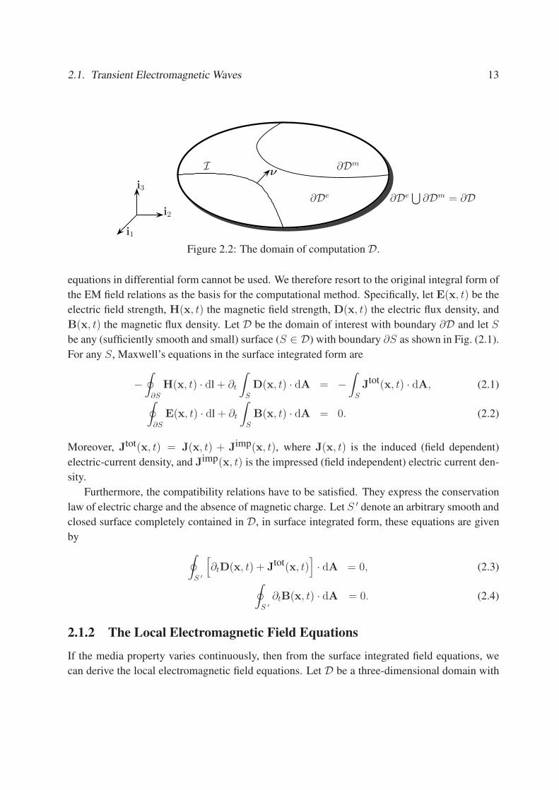
2.1. Transient Electromagnetic Waves 13
Iν
∂Dm
∂De ∂De⋃
∂Dm = ∂D
i1
i2
i3
Figure 2.2: The domain of computation D.
equations in differential form cannot be used. We therefore resort to the original integral form of
the EM field relations as the basis for the computational method. Specifically, let E(x, t) be the
electric field strength, H(x, t) the magnetic field strength, D(x, t) the electric flux density, and
B(x, t) the magnetic flux density. Let D be the domain of interest with boundary ∂D and let S
be any (sufficiently smooth and small) surface (S ∈ D) with boundary ∂S as shown in Fig. (2.1).
For any S, Maxwell’s equations in the surface integrated form are
−∮
∂S
H(x, t) · dl + ∂t
∫
S
D(x, t) · dA = −∫
S
Jtot(x, t) · dA, (2.1)
∮
∂S
E(x, t) · dl + ∂t
∫
S
B(x, t) · dA = 0. (2.2)
Moreover, Jtot(x, t) = J(x, t) + Jimp(x, t), where J(x, t) is the induced (field dependent)
electric-current density, and Jimp(x, t) is the impressed (field independent) electric current den-
sity.
Furthermore, the compatibility relations have to be satisfied. They express the conservation
law of electric charge and the absence of magnetic charge. Let S ′ denote an arbitrary smooth and
closed surface completely contained in D, in surface integrated form, these equations are given
by
∮
S ′
[∂tD(x, t) + Jtot(x, t)
]· dA = 0, (2.3)
∮
S ′
∂tB(x, t) · dA = 0. (2.4)
2.1.2 The Local Electromagnetic Field Equations
If the media property varies continuously, then from the surface integrated field equations, we
can derive the local electromagnetic field equations. Let D be a three-dimensional domain with

14 Chapter 2. The Electromagnetic Field Equations
an interface I as indicated in Fig. (2.2). In a domain where the spatial electromagnetic properties
of the media vary continuously (D\I), the electromagnetic field satisfies the following system
of first-order partial differential equations, which can actually be derived from Eq. (2.1) and
Eq. (2.2).
−∇× H(x, t) + ∂tD(x, t) = −Jtot(x, t) for x ∈ (D\I), (2.5)
∇×E(x, t) + ∂tB(x, t) = 0 for x ∈ (D\I). (2.6)
These two equations are known as Ampere’s law and Faraday’s law in differential form.
Similarly, we can derive from the surface integrated compatibility equations the compatibility
equations in differential form:
∇ ·[∂tD(x, t) + Jtot(x, t)
]= 0 for x ∈ (D\I), (2.7)
∇ · ∂tB(x, t) = 0 for x ∈ (D\I). (2.8)
These equations are called the local compatibility relations, and they are automatically satisfied
by the correct solution of Maxwell’s equations.
2.1.3 Constitutive Relations
Maxwell’s equations alone are not sufficient to determine the electromagnetic field, constitutive
relations are needed to define the electromagnetic properties of media and relate different field
quantities.
Although more complicated constitutive relations may hold, we assume in this thesis that
the media present in the configurations are linear, time-invariant, possibly inhomogeneous and
locally-reacting. Let ε be the electric permittivity, σ be the electric conductivity, and µ the
magnetic permeability, the constitutive relations are then
D(x, t) = ε(x)E(x, t), J(x, t) = σ(x)E(x, t),
Jtot(x, t) = J(x, t) + Jimp(x, t), B(x, t) = µ(x)H(x, t).
2.1.4 Interface Conditions
At the interface I between two media both taking different values in their electromagnetic ma-
terial parameters when approaching I from either side, i.e. at least one of the constitutive pa-
rameters changes abruptly when crossing I, Eq. (2.5) and Eq. (2.6) do not hold because the
field quantities are no longer differentiable. In the absence of surface currents and charges at
the interface, the field quantities must satisfy the following two physical requirements [41] upon
crossing the interface. (1) The first physical requirement is the continuity of the components of

2.1. Transient Electromagnetic Waves 15
the electric and magnetic field strengths tangential to the interface, that is:
ν ×H(x, t) is continuous across I, (2.9)
ν ×E(x, t) is continuous across I, (2.10)
where ν is the unit vector perpendicular to I, as indicated in Fig. (2.2). The normal components
of the electric and magnetic field strengths (the components perpendicular to the interface) are
free to jump across I. (2) The second physical requirement is the continuity of the components
of the total volume density of electric and magnetic currents normal to the interface, that is:
ν ·[∂tD(x, t) + Jtot(x, t)
]is continuous across I, (2.11)
ν · B(x, t) is continuous across I. (2.12)
The tangential components (the components tangential to the interface) are free to jump across
I. These interface conditions follow from the Maxwell equations in integral form [26, 55].
2.1.5 Initial Condition and Boundary Conditions
In a computational domain D bounded by ∂D, uniqueness of the field solutions of Maxwell’s
equations is ensured if the correct initial condition and boundary conditions are prescribed. We
first discuss the initial conditions. Subsequently, the boundary conditions at the external bound-
ary ∂D, which is assumed to be smooth, are expressed through the tangential components of the
electric and/or magnetic field strengths.
Initial Condition
Throughout this thesis, we assume that valid initial electromagnetic field strengths, which satisfy
Maxwell’s equations, the compatibility equations, interface equations and boundary conditions,
are known. For most cases, it is sufficient to assume that the domain of interest D is initially at
rest. This implies vanishing electromagnetic field quantities before the switch-on of any sources
in the spatial domain.
Boundary Conditions
The boundary conditions at the outer boundary ∂D can be defined by either prescribing the
tangential components of the electric field strength or magnetic field strength. Uniqueness of the
electromagnetic wave solutions in a bounded domain can be proved if the tangential component
of the electric or the magnetic field strength is prescribed on the outer boundary ∂D (e.g. by A.T.
de Hoop in [57]). Mixed boundary conditions, i.e. prescribed tangential electric field strength
on parts of ∂D forming ∂De, and prescribed tangential magnetic field strength on the rest of ∂D

16 Chapter 2. The Electromagnetic Field Equations
forming ∂Dm, is also possible as long as ∂De ∪∂Dm = ∂D and ∂De ∩∂Dm = ∅. In the absenceof any surface currents and charges, we can write down the boundary conditions as
ν × H(x, t) = ν ×Hext(x, t), for x ∈ ∂Dm, (2.13)
ν × E(x, t) = ν ×Eext(x, t), for x ∈ ∂De, (2.14)
where ν is the outwardly directed unit vector normal to ∂D,Eext(x, t),x ∈ ∂De andHext(x, t),x ∈∂Dm are the prescribed field strengths on the boundaries. In the special case where
ν ×E(x, t) = 0, for x ∈ ∂De,
is referred to as a Perfect Electric Conductor (PEC) boundary condition. Similarly, if
ν ×H(x, t) = 0, for x ∈ ∂Dm,
we refer to it as a Perfect Magnetic Conductor (PMC) boundary condition.
2.1.6 Absorbing Boundary Conditions in the Time Domain
For electromagnetic wave computation, the unbounded problemwhere the computational domain
extends to infinity must be modeled. In this thesis, we adopt the analysis and Perfectly Matched
Layers discussed by A. T. de Hoop et al. in [58]. For the experimental result in the time domain,
please refer to Section 5.3.4.
2.2 Maxwell’s Equations in the Frequency Domain
When assuming the media to be linear time invariant, we may apply a Fourier transform to
Ampere’s and Faraday’s equations. In practice we replace ∂t with jω, where ω = 2πf is the
angular frequency. Then we have the field equations in the frequency domain for fields in steady
state.
2.2.1 The Surface Integrated Field Equations in the Frequency Domain
Let D be the domain of interest with boundary ∂D, S be any (sufficiently smooth and small)
surface (S ∈ D) with boundary ∂S in D. For any S Maxwell’s equations in the frequency
domain in surface integrated form are:
∮
∂S
H(x, ω) · dl = jω
∫
S
D(x, ω) · dA +
∫
S
Jtot(x, ω) · dA, (2.15)
∮
∂S
E(x, ω) · dl = −jω
∫
S
B(x, ω) · dA. (2.16)

2.2. Maxwell’s Equations in the Frequency Domain 17
Let S ′ be a close surface in D, the surface integrated compatibility relations are∮
S ′
[jωD(x, ω) + Jtot(x, ω)
]· dA = 0, (2.17)
∮
S ′
B(x, ω) · dA = 0, (2.18)
where ν is the unit vector perpendicular to the surface S ′ and is outwardly oriented. The above
compatibility equations are easily derived from Eqs. (2.15) and (2.16).
2.2.2 The Local Electromagnetic Field Equations for Harmonic Waves
Let D be a three dimensional domain with interface I as indicated in Fig. (2.2), in a domain
where the spatial electromagnetic properties of the medium vary continuously (D\I), the elec-
tromagnetic field satisfies the following system of first-order partial differential equations which
are actually derived from Eqs. (2.15) and (2.16):
−∇×H(x, ω) + jωD(x, ω) = −Jtot(x, ω) for x ∈ (D\I), (2.19)
∇× E(x, ω) + jωB(x, ω) = 0 for x ∈ (D\I). (2.20)
Similarly, we have the local compatibility relations:
∇ ·[jωD(x, ω) + Jtot(x, ω)
]= 0 for x ∈ (D\I), (2.21)
∇ · B(x, ω) = 0 for x ∈ (D\I). (2.22)
They are automatically satisfied by the correct solution of Maxwell’s equations.
2.2.3 Constitutive Relations
As stated before and for simplicity, we assume that the media present in the configurations are
linear, time-invariant, possibly inhomogeneous, isotropic and non-dynamic. Specifically, the
constitutive relations are then
D(x, ω) = ε(x)E(x, ω), J(x, ω) = σ(x)E(x, ω),
Jtot(x, ω) = J(x, ω) + Jext(x, ω), B(x, ω) = µ(x)H(x, ω).
2.2.4 Interface Conditions and Boundary Conditions
The interface conditions and boundary conditions for the electromagnetic fields in the frequency
domain are parallel to those in the time domain. For electromagnetic wave computation, the
unbounded problems where the computational domain extends to infinity must be modeled. In
this thesis we adopt the analysis and Perfectly Matched Layers discussed by A. T. de Hoop et al.
in [58]. Please refer to Section 5.2.2 for experimental results on Perfectly Matched Layers in the
frequency domain.

18 Chapter 2. The Electromagnetic Field Equations
Table 2.1: Correspondence between generic quantities and the actual static and stationary field
values (linear media is assumed)
Generic form stationary electric cases static electric cases stationary magnetic cases
V E E H
F J D B
ξ σ ε µ
Qimp 0 0 Jtot
QimpS 0 0 J
impS
ρimp −∇ · Jimp ρ 0
σimp − ν · Jimp∣∣∣2
1σe 0
Vext Eext Eext Hext
σext ν · Jext ν · Dext ν · Bext
2.3 Stationary and Static Field Equations
When the field quantities do not vary in time, the time-derivative of the field quantities van-
ishes, and we have a static or stationary field. Static means that the electric charge is static and
stationary means that the electric charge flows at a constant rate. In these cases, there is no in-
teraction between the electric and magnetic field. The electro-stationary case, electrostatic case
and magnetostatic case can then be solved separately.
The equations for static and stationary electric and magnetic fields have essentially the same
form. Therefore, with the mapping of Tab. 2.1, we may represent all static and stationary field
equations in a generic form.
2.3.1 Basic Equations
Let V(x) represent either E(x) or H(x), Qimp(x) represent the impressed volume current den-
sity, either 0 or Jtot(x), the surface integrated field equation can be simplified as:
∮
∂S
V(x) · dl =
∫
S
Qimp(x) · dA. (2.23)
If V(x) is differentiable, we have the local equation:
∇× V(x) = Qimp(x), x ∈ D/I. (2.24)

2.3. Stationary and Static Field Equations 19
2.3.2 The Generic Constitutive Relations
Let F(x) represent either J(x), D(x) or B(x), and ξ(x) represent the material parameter in case
of linear media. Although more complicated relations can be considered, we only consider linear
non-dynamic media in this thesis, that is:
F(x) = ξ(x)V(x). (2.25)
2.3.3 Compatibility Relations
Let ρimp(x) be the impressed volume charge density. It represents either−∇·Jimp(x), ρ(x) or
0. The generic compatibility relation that applies for static and stationary electric and magnetic
fields in surface integrated form is:
∮
∂V
F(x) · dA =
∮
V
ρimp(x)dV. (2.26)
If F(x) is differentiable, we have the local equation:
∇ · F(x) = ρimp(x),x ∈ D/I. (2.27)
2.3.4 Interface Conditions
Similarly, let ν × V(x)|21 denote the jump in the tangential component of the field strength across
the interface between media 1 and 2, and ν · F(x)|21 denote the jump in the normal component
of the flux density across the interface between 1 and 2, the generic static and stationary interface
conditions are:
ν × V(x)|21 = QimpS (x), x ∈ I, (2.28)
ν · F(x)|21 = σimp(x), x ∈ I. (2.29)
2.3.5 Boundary Conditions
As for the boundary conditions, let ∂DV ∪ ∂DF = ∂D and ∂DV ∩ ∂DF = ∅, we have:
ν × V(x) = ν × Vext(x), x ∈ ∂DV, (2.30)
ν · F(x) = σext(x), x ∈ ∂DF, (2.31)
where ν×Vext(x) denotes the tangential component of the electric field strength or the magnetic
field strength on the exterior boundary, σext(x) denotes the normal component of the electric
current density, the electric flux density or magnetic flux density on the exterior boundary.

20 Chapter 2. The Electromagnetic Field Equations
2.4 Discussion
Although people are more familiar with the Maxwell equations in differential form, these equa-
tions are not valid in case of discontinuity where the electromagnetic field strengths are not
differentiable. The Maxwell equations in integral form, on the other hand, are always valid, and
they only require the field to be integrable. That is why we adopt the integral equations as the
basis for our computational method.
In addition to the Maxwell equations, the compatibility relations, boundary conditions and
interface conditions are also very important. In this chapter, we have introduced the surface
integrated field equations which are the bases of our computational method. In the next chapter,
we are going to demonstrate how we discretize the field quantities in these equations.

Chapter 3
Spatial Discretization of the Field Quantities
Science is built of facts the way a house is built of bricks; but
an accumulation of facts is no more science than a pile of
bricks is a house.
Henri Poincare
In this chapter, we present a spatial discretization scheme for discretizing the field quan-
tities in the domain of interest. First we discuss the geometric properties and the geometric
specifications of the finite element in Section 3.1, and then the expression for the scalar linear,
interpolation function (Section 3.2), which is used in deriving the expansion functions for the
electromagnetic field quantities in Section 3.3.
3.1 The Tetrahedron as a Finite Element
In the numerical methods based on finite elements (we use the term “finite element” to refer
to the elementary sub-domain of a mesh and not in the more restricted sense of “Galerkin Fi-
nite Elements” sometimes used in the literature), the spatial domain of computation is firstly
geometrically discretized into elementary sub-domains. The maximum diameter (denoted as h
throughout this thesis) of these elementary domains is taken to be sufficiently small such that
simple functions can represent the spatial variations of the electromagnetic field quantities over
it. For versatility and generality, we take the tetrahedron, the simplex in the space ℜ3, as the
elementary geometrical sub-domain for three-dimensional domains of computation.
3.1.1 Basic Symbols on the Triangulation
We introduce the following symbols to represent tetrahedron related quantities:
• We refer to an unspecified open tetrahedron as T .
• Let ∂T be the surface delimiting the tetrahedron T . ∂T consists of four faces, six edges
and four nodes that delimit the relevant tetrahedron.
• T = T ∪ ∂T denotes the closure of the tetrahedron T .
21

22 Chapter 3. Spatial Discretization of the Field Quantities
• NT denotes the total number of tetrahedrons in the triangulation.
• The tetrahedrons in the triangulation are labeled by a set of global tetrahedron indexes
IT = n; n = 1, 2, ..., NT .
• T (n) denotes a specific tetrahedron with global index n.
• The tetrahedron mesh or simply the triangulation:⋃NT
n=1 T (n).
• T = T (n); n = 1, ..., NT denotes the set of all tetrahedrons in the triangulation.
3.1.2 Requirements on the Triangulation
The triangulation must satisfy the following set of requirements.
1. Each tetrahedron in the triangulation has a non-empty interior.
2. The union of the closures of all simplexes must span the whole domain of computation
exactly, when the domain of computation D is a polyhedron. Otherwise this union must
approximate the domain of computation, that is,
D = ∂D⋃
D ≈NT⋃
n=1
T (n). (3.1)
3. For any two different tetrahedrons T (n1) and T (n2) with n1/=n2, T (n1)⋂T (n2) = ∅.
4. Any face of a tetrahedron T (n1) ∈ T is either a subset of the domain of computation’s
outer boundary ∂D or a face of another tetrahedron T (n2) ∈ T, n2/=n1.
5. Throughout this dissertation, we assume that the material interface of the domain coincides
with the faces of tetrahedrons, in other words, the triangulation is interface-conforming.
3.1.3 Geometric Properties of the Tetrahedron
Given an arbitrary tetrahedron T (n) in T, its geometric information is defined separately below.
The Four Nodes Delimiting a Tetrahedron
The nodes delimiting a tetrahedron can be identified by means of local node indexes.
• The four nodes delimiting an arbitrary tetrahedron T (n) are locally labeled as 0, 1, 2, 3and we may refer to these nodes by local labels, i.e. N (n, 0), N (n, 1), N (n, 2), N (n, 3)
(see Fig. 3.1).

3.1. The Tetrahedron as a Finite Element 23
N (n, i)
N (n, j)
N (n, k)
N (n, l)
E(n, i, j)E(n, j, k)
F(n, k)
Figure 3.1: Tetrahedron T (n) and some of its locally defined geometric elements. Here,
(i, j, k, l) is an even permutation of (0, 1, 2, 3), which forms a right-handed system.
• The position vectors of the nodes with respect to the background Cartesian reference frame
are given by x(n, 0),x(n, 1),x(n, 2),x(n, 3) as shown in Fig. (3.2).
• The total number of nodes in the triangulation is NN .
• The nodes are numbered throughout the triangulation by a set of global node indexes, i.e.
IN = m; m = 1, 2, ..., NN.
• A globally labeled node with global index m is denoted by N (m).
• The position vector of a globally labeled nodeN (m)with respect to the background Carte-
sian reference frame is denoted by x(m).
• Given a combination of a tetrahedron index and a local node index (n, i), the global node
index of the node is uniquely determined as m. Reversely, given a combination of a global
node index m and a tetrahedron index n, the local vertex index i is uniquely determined, if
the given nodeN (m) delimits the tetrahedron T (n).
The Six Vectorial Edges Delimiting a Tetrahedron
Let (i, j, k, l) be an even permutation of (0, 1, 2, 3) and n ∈ IT . The edge delimited by the nodes i
and j of a tetrahedron T (n) and oriented fromN (n, i) toN (n, j) is locally denoted by E(n, i, j)
as indicated in Fig. (3.1). Its associated vectorial edge e(n, i, j) is given by
e(n, i, j) = x(n, j) − x(n, i),

24 Chapter 3. Spatial Discretization of the Field Quantities
x(n, i)
x(n, j)
x(n, k)
x(n, l)
e(n, i, j)e(n, j, k)
A(n, k)
Figure 3.2: Vectorial coordinate of the four nodes, vectorial edges, and vectorial faces delimiting
the tetrahedron T (n). Here, (i, j, k, l) is an even permutation of (0, 1, 2, 3), where (0, 1, 2, 3)
forms a right-handed system.
as indicated in Fig. (3.2). For example, three vectorial edges are mathematically given by
e (n, 0, 1) = x(n, 1) − x(n, 0),
e (n, 1, 2) = x(n, 2) − x(n, 1),
e (n, 2, 0) = x(n, 0) − x(n, 2). (3.2)
Taking the sum of these vectorial edges yields
e (n, 0, 1) + e (n, 1, 2) + e (n, 2, 0) = 0,
as expected for a closed path.
Let the global node indexes of N (n, i) and N (n, j) be m and u, respectively, and let m, u ∈IN , then the edge can be globally denoted by E(m, u). Its associated vectorial edge e(m, u) is
given by,
e(m, u) = x(u) − x(m).
Note that the nodesN (n, 0),N (n, 1) and N (n, 2) define a plane in which vectors E(n, 0, 1)
and E(n, 0, 2) are lying. The operation of the cross product e(n, 0, 1)×e(n, 0, 2) produces a vec-
tor perpendicular to the plane containingN (n, 0),N (n, 1) andN (n, 2). If the nodeN (n, 3) lies
on the side of the plane containing N (n, 0), N (n, 1) and N (n, 2) where e(n, 0, 1) × e(n, 0, 2)
points, we say the nodes numbering proceeds “right-handed” around the tetrahedron. Through-
out this thesis, we assume the nodes of each tetrahedron element are numbered “right-handed”
around the tetrahedron.

3.1. The Tetrahedron as a Finite Element 25
The Four Oriented Faces Delimiting a Tetrahedron
Assuming a right-handed system, let (i, j, k, l) be an even permutation of (0, 1, 2, 3) and n ∈ IT .
The plane face delimited by the nodes i, j and l of the tetrahedron T (n) is denoted locally by
F(n, k) as indicated in Fig. (3.1). Two vectorial faces perpendicular to this face can be defined,
i.e. the vector on the face perpendicular to it and directed away from nodeN (n, k) and the vector
on the face perpendicular to it and directed to nodeN (n, k). Throughout this thesis, the vectorial
face is chosen positively directed away from N (n, k) and it is denoted by A(n, k) as indicated
in Fig. (3.2). The four vectorial faces are:
A (n, 0) =1
2[e (n, 1, 2) × e (n, 1, 3)] ,
A (n, 1) =1
2[e (n, 0, 3) × e (n, 0, 2)] ,
A (n, 2) =1
2[e (n, 3, 0) × e (n, 3, 1)] ,
A (n, 3) =1
2[e (n, 2, 1) × e (n, 2, 0)] . (3.3)
Taking the sum of these vectorial faces we have
A (n, 0) + A (n, 1) + A (n, 2) + A (n, 3) = 0, (3.4)
which implies that ∂T forms a closed boundary.
The Barycenter
The barycenter xb(n) of the tetrahedron T (n) is defined as:
xb(n) =1
4[x(n, 0) + x(n, 1) + x(n, 2) + x(n, 3)] .
The Volume of a Tetrahedron
The volume of the tetrahedron T (n) can be computed with the formula
V (n) =1
3[e (n, i, j) · A (n, i)] , (3.5)
or equivalently:
V (n) =1
3det
1 x1(n, 0) x2(n, 0) x3(n, 0)
1 x1(n, 1) x2(n, 1) x3(n, 1)
1 x1(n, 2) x2(n, 2) x3(n, 2)
1 x1(n, 3) x2(n, 3) x3(n, 3)
. (3.6)
The local ordering of vertexes should always keep the volume positive.

26 Chapter 3. Spatial Discretization of the Field Quantities
3.2 The Linear Expansion Functions
A computational method based on finite elements requires that the domain is discretized and
the physical quantities are approximated by interpolation over values defined on the discretized
domain. This interpolation is carried out with expansion functions also known as interpolation
functions or approximation functions. The discrete field quantities have certain values at specific
locations in the domain of computation i.e. on nodes or edges. To obtain a value at any other
location, one needs to use a set of expansion functions to approximate the value at the location
of interest based on the values at specific node or edge locations. For the sake of efficiency and
simplicity, the expansion functions are usually polynomial functions with small support, i.e. they
are non-zero for a (relatively) small sub-domain of D. As a starting point, we will introduce the
linear local scalar interpolation functions and linear local nodal interpolation functions, along
with their properties.
3.2.1 The Linear Scalar Interpolation Function
Let x be a position vector of a point in the closure of a tetrahedron T (n), that is, x ∈ T (n).
Definition 3.1. The linear interpolation function is defined as:
φ(x, n, i) =1
4− [x − xb(n)] · A(n, i)
3V (n), for n ∈ IT , i = 0, 1, 2, 3,x ∈ T (n). (3.7)
The local scalar interpolation functions have the following properties [29, 26]:
1. φ(x, n, i) takes the value ‘1’ at the node N (n, i) and the value ‘0’ at the remaining nodes.
2. A summation over all i = 0, 1, 2, 3 in Eq. (3.7) and application of Eq. (3.4) yields:
3∑
i=0
φ(x, n, i) = 1 for n ∈ IT , x ∈ T (n).
3. For all faces delimiting the tetrahedron T (n), i.e. F(n, i), i = 0, 1, 2, 3;
φ(x, n, i) = 0 for n ∈ IT , i = 0, 1, 2, 3, x ∈ F(n, i).
4. The gradient of the interpolation function is constant throughout T (n) and has the value
∇φ(x, n, i) = −A(n, i)
3V (n), for n ∈ IT , i = 0, 1, 2, 3, x ∈ T (n). (3.8)
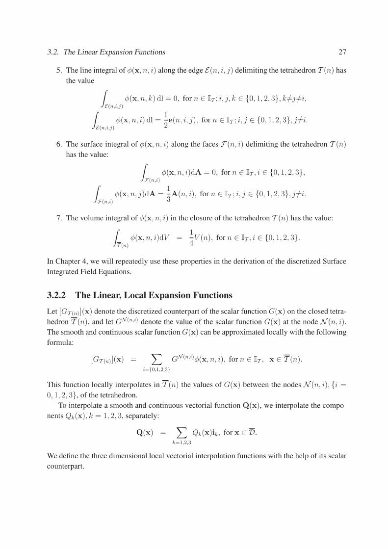
3.2. The Linear Expansion Functions 27
5. The line integral of φ(x, n, i) along the edge E(n, i, j) delimiting the tetrahedron T (n) has
the value∫
E(n,i,j)
φ(x, n, k) dl = 0, for n ∈ IT ; i, j, k ∈ 0, 1, 2, 3, k/=j /=i,
∫
E(n,i,j)
φ(x, n, i) dl =1
2e(n, i, j), for n ∈ IT ; i, j ∈ 0, 1, 2, 3, j /=i.
6. The surface integral of φ(x, n, i) along the faces F(n, i) delimiting the tetrahedron T (n)
has the value:∫
F(n,i)
φ(x, n, i)dA = 0, for n ∈ IT , i ∈ 0, 1, 2, 3,∫
F(n,i)
φ(x, n, j)dA =1
3A(n, i), for n ∈ IT ; i, j ∈ 0, 1, 2, 3, j /=i.
7. The volume integral of φ(x, n, i) in the closure of the tetrahedron T (n) has the value:∫
T (n)
φ(x, n, i)dV =1
4V (n), for n ∈ IT , i ∈ 0, 1, 2, 3.
In Chapter 4, we will repeatedly use these properties in the derivation of the discretized Surface
Integrated Field Equations.
3.2.2 The Linear, Local Expansion Functions
Let [GT (n)](x) denote the discretized counterpart of the scalar function G(x) on the closed tetra-
hedron T (n), and let GN (n,i) denote the value of the scalar function G(x) at the node N (n, i).
The smooth and continuous scalar function G(x) can be approximated locally with the following
formula:
[GT (n)](x) =∑
i=0,1,2,3
GN (n,i)φ(x, n, i), for n ∈ IT , x ∈ T (n).
This function locally interpolates in T (n) the values of G(x) between the nodes N (n, i), i =
0, 1, 2, 3, of the tetrahedron.To interpolate a smooth and continuous vectorial function Q(x), we interpolate the compo-
nents Qk(x), k = 1, 2, 3, separately:
Q(x) =∑
k=1,2,3
Qk(x)ik, for x ∈ D.
We define the three dimensional local vectorial interpolation functions with the help of its scalar
counterpart.

28 Chapter 3. Spatial Discretization of the Field Quantities
Definition 3.2. The local vectorial interpolation functions are defined as
Φk(x, n, i) = φ(x, n, i)ik, for n ∈ IT ,x ∈ T (n), k = 1, 2, 3. (3.9)
With Eq.(3.8), the curl and divergence of the local vectorial interpolation functions are con-
stant throughout T (n) and they have the values:
∇× Φk(x, n, i) = −A(n, i) × ik
3V (n), for n ∈ IT ,x ∈ T (n), k = 1, 2, 3,
∇ · Φk(x, n, i) = −A(n, i) · ik3V (n)
, for n ∈ IT ,x ∈ T (n), k = 1, 2, 3. (3.10)
Let [QT (n)](x) be the discrete counterpart of the vectorial function Q(x) in the closure of a tetra-
hedron T (n), the vectorial function Q(x) can be expanded locally with the following formula:
[QT (n)](x) =∑
i=0,1,2,3
∑
k=1,2,3
[Q
N (n,i)k Φk(x, n, i)
], for n ∈ IT ,x ∈ T (n), (3.11)
where QN (n,i)k denotes the value of the kth component of the vectorial function Q(x) at the node
N (n, i), i.e. QN (n,i).
3.2.3 The Linear, Nodal Expansion Functions
In order to construct the linear, nodal expansion functions (also known as Cartesian expansion
functions) of Q(x) from the linear, local expansion function, we introduce the characteristic
function χT (n)(x) associated with the tetrahedron T (n),
Definition 3.3. The characteristic function χT (n)(x) is defined as:
χT (n)(x) =
1 for x ∈ T (n),
undefined for x ∈ ∂T (n),
0 otherwise.
(3.12)
Note that the characteristic function is undefined on the boundary of tetrahedrons, because
these boundaries can be on an interface of discontinuity. There, the field strengths may not be
well defined. Using this definition, we extend the linear, local Cartesian expansion given by
Eq. (3.11) to the domain of computation and then take the sum over all tetrahedrons:
[Q](x) =∑
n∈IT
3∑
i=0
3∑
k=1
[Q
N (n,i)k Φk(x, n, i) χT (n)(x)
], for x ∈ D,
with continuity extension as required by the continuity conditions. (3.13)
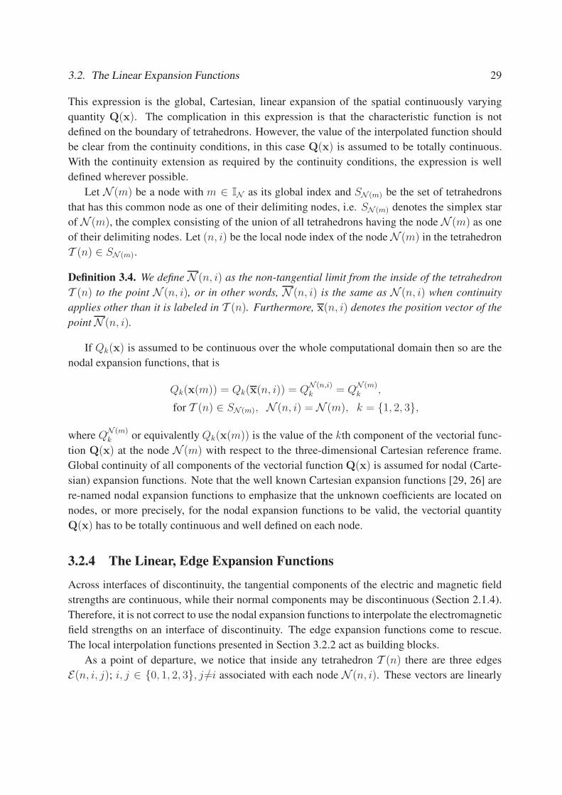
3.2. The Linear Expansion Functions 29
This expression is the global, Cartesian, linear expansion of the spatial continuously varying
quantity Q(x). The complication in this expression is that the characteristic function is not
defined on the boundary of tetrahedrons. However, the value of the interpolated function should
be clear from the continuity conditions, in this case Q(x) is assumed to be totally continuous.
With the continuity extension as required by the continuity conditions, the expression is well
defined wherever possible.
Let N (m) be a node with m ∈ IN as its global index and SN (m) be the set of tetrahedrons
that has this common node as one of their delimiting nodes, i.e. SN (m) denotes the simplex star
of N (m), the complex consisting of the union of all tetrahedrons having the node N (m) as one
of their delimiting nodes. Let (n, i) be the local node index of the nodeN (m) in the tetrahedron
T (n) ∈ SN (m).
Definition 3.4. We define N (n, i) as the non-tangential limit from the inside of the tetrahedron
T (n) to the point N (n, i), or in other words, N (n, i) is the same as N (n, i) when continuity
applies other than it is labeled in T (n). Furthermore, x(n, i) denotes the position vector of the
pointN (n, i).
If Qk(x) is assumed to be continuous over the whole computational domain then so are the
nodal expansion functions, that is
Qk(x(m)) = Qk(x(n, i)) = QN (n,i)k = Q
N (m)k ,
for T (n) ∈ SN (m), N (n, i) = N (m), k = 1, 2, 3,
where QN (m)k or equivalently Qk(x(m)) is the value of the kth component of the vectorial func-
tion Q(x) at the node N (m) with respect to the three-dimensional Cartesian reference frame.
Global continuity of all components of the vectorial function Q(x) is assumed for nodal (Carte-
sian) expansion functions. Note that the well known Cartesian expansion functions [29, 26] are
re-named nodal expansion functions to emphasize that the unknown coefficients are located on
nodes, or more precisely, for the nodal expansion functions to be valid, the vectorial quantity
Q(x) has to be totally continuous and well defined on each node.
3.2.4 The Linear, Edge Expansion Functions
Across interfaces of discontinuity, the tangential components of the electric and magnetic field
strengths are continuous, while their normal components may be discontinuous (Section 2.1.4).
Therefore, it is not correct to use the nodal expansion functions to interpolate the electromagnetic
field strengths on an interface of discontinuity. The edge expansion functions come to rescue.
The local interpolation functions presented in Section 3.2.2 act as building blocks.
As a point of departure, we notice that inside any tetrahedron T (n) there are three edges
E(n, i, j); i, j ∈ 0, 1, 2, 3, j /=i associated with each node N (n, i). These vectors are linearly

30 Chapter 3. Spatial Discretization of the Field Quantities
QEn,i,j(x(n, i))
QEn,i,k(x(n, i))
QEn,i,l(x(n, i))
N (n, i)
N (n, j)
N (n, k)
N (n, l)
Figure 3.3: The scalar function Q(x) on the four nodes delimiting the tetrahedron T (n).
independent for any non-degenerated tetrahedron and form a three-dimensional base (hereafter,
referred as the edge base) for the representation of the three dimensional space just like the
Cartesian bases. With a base transformation, we can represent the three-dimensional vectorial
function Q(x) in the edge base associated with the node N (n, i) in the tetrahedron T (n) as
Q(x) =∑
k=1,2,3
Qk(x)ik
=∑
j=0,1,2,3,j/=i
[(Q(x) · e(n, i, j)
|e(n, i, j)|
)(−|e(n, i, j)|
3V (n)A(n, j)
)]. (3.14)
Now, with Eq. (3.14), we can represent the vectorial function Q(x) on each of the four nodes
N (n, i), i = 0, 1, 2, 3 of the tetrahedron T (n) with the edge base on each node, that is,
QN (n,i) =∑
k=1,2,3
QN (n,i)k ik
=∑
j=0,1,2,3,j/=i
[(QN (n,i) · e(n, i, j)
|e(n, i, j)|
)(−|e(n, i, j)|
3V (n)A(n, j)
)].
Substituting the above equation into Eq. (3.11) and using Eq. (3.9), we obtain:
[QT (n)](x) =
3∑
i=0
3∑
k=1
[Q
N (n,i)k Φk(x, n, i)
]
=
3∑
i=0
∑
j=0,1,2,3j/=i
[(QN (n,i) · e(n, i, j)
|e(n, i, j)|
)(−|e(n, i, j)|
3V (n)A(n, j)
)φ(x, n, i)
].(3.15)
We recognize a part of the above equation as the projection of Q(x(n, i)) along the direction of
the edge E(n, i, j), that is,
QE(n,i,j) = Q(x(n, i)) · e(n, i, j)
|e(n, i, j)| ,

3.2. The Linear Expansion Functions 31
where QE(n,i,j) denotes the projection of Q(x(n, i)) along the direction of the edge E(n, i, j).
We can then extend the local expansion functions to the entire computational domainD with
the help of characteristic functions, and then a summation over all tetrahedrons yields the discrete
representation of the vectorial function Q(x). Specifically, we have
[Q](x) =
NT∑
n=1
3∑
i=0
∑
j=0,1,2,3j/=i
[QE(n,i,j)
(−|e(n, i, j)|
3V (n)A(n, j)
)φ(x, n, i)χT (n)(x)
],
for x ∈ D,with continuity extension as required by the continuity conditions.
Now, let m and u be the global node indexes of the nodes N (n, i) and N (n, j) and let QE(m,u)
denote the projection of a vectorial function Q(x) at the point N (m) along the direction of the
edge E(m, u). To ensure tangential continuity, QE(m,u) must be uniquely defined, that is,
Q(x(n, i)) · e(n, i, j)
|e(n, i, j)| = QE(m,u) = QE(n,i,j),
for n ∈ IT ; m, u ∈ IN , Tn ∈ SE(m,u), E(n, i, j) = E(m, u), (3.16)
where SE(m,u) denotes the set of tetrahedrons which share the common edge E(m, u).
3.2.5 Properties of the Linear, Nodal and Edge Expansion Functions
Each of the two expansion functions has advantages and weaknesses. In this section, we present
a comparison between them. It will be clear from Section 5.1 that only the right combination of
these two expansion functions would win in terms of accuracy and efficiency. A list of properties
of the linear nodal and edge expansion functions follows:
• Both of the two expansion functions are consistently linear functions [22]. They permit a
consistently linear expansion of a vectorial function Q(x) in each tetrahedron. In contrast
to constant linear edge element e.g. Whitney’s linear element [59], of which the approx-
imation error is of order O(h) [15], the approximation errors of both expansion functions
are of order O(h2), which we shall show experimentally in Chapter 5.
• To interpolate a vectorial function Q(x), the nodal expansion functions require three un-
known coefficients per node and the edge expansion functions require one unknown coef-
ficient for each edge emerging from each node. For topological reasons, there are at least
three edges (usually much more) emerging from each node, therefore more coefficients or
degrees of freedom (DOF) are needed for edge expansion functions. In other words, the
edge expansion functions are more computationally expensive than the nodal expansion
functions.
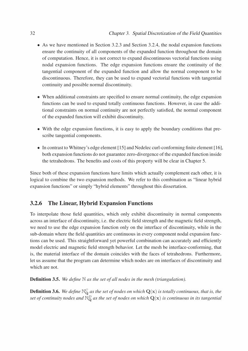
32 Chapter 3. Spatial Discretization of the Field Quantities
• As we have mentioned in Section 3.2.3 and Section 3.2.4, the nodal expansion functions
ensure the continuity of all components of the expanded function throughout the domain
of computation. Hence, it is not correct to expand discontinuous vectorial functions using
nodal expansion functions. The edge expansion functions ensure the continuity of the
tangential component of the expanded function and allow the normal component to be
discontinuous. Therefore, they can be used to expand vectorial functions with tangential
continuity and possible normal discontinuity.
• When additional constraints are specified to ensure normal continuity, the edge expansion
functions can be used to expand totally continuous functions. However, in case the addi-
tional constraints on normal continuity are not perfectly satisfied, the normal component
of the expanded function will exhibit discontinuity.
• With the edge expansion functions, it is easy to apply the boundary conditions that pre-
scribe tangential components.
• In contrast toWhitney’s edge element [15] and Nedelec curl-conforming finite element [16],
both expansion functions do not guarantee zero-divergence of the expanded function inside
the tetrahedrons. The benefits and costs of this property will be clear in Chapter 5.
Since both of these expansion functions have limits which actually complement each other, it is
logical to combine the two expansion methods. We refer to this combination as “linear hybrid
expansion functions” or simply “hybrid elements” throughout this dissertation.
3.2.6 The Linear, Hybrid Expansion Functions
To interpolate those field quantities, which only exhibit discontinuity in normal components
across an interface of discontinuity, i.e. the electric field strength and the magnetic field strength,
we need to use the edge expansion function only on the interface of discontinuity, while in the
sub-domain where the field quantities are continuous in every component nodal expansion func-
tions can be used. This straightforward yet powerful combination can accurately and efficiently
model electric and magnetic field strength behavior. Let the mesh be interface-conforming, that
is, the material interface of the domain coincides with the faces of tetrahedrons. Furthermore,
let us assume that the program can determine which nodes are on interfaces of discontinuity and
which are not.
Definition 3.5. We define N as the set of all nodes in the mesh (triangulation).
Definition 3.6. We define NCQ as the set of nodes on which Q(x) is totally continuous, that is, the
set of continuity nodes and NDQ as the set of nodes on which Q(x) is continuous in its tangential

3.2. The Linear Expansion Functions 33
QE(n,i,j)
QE(n,i,k)
QE(n,i,l)
QN (n,l)1 i1
QN (n,l)2 i2
QN (n,l)3 i3
N (n, i)
N (n, j)
N (n, k)
N (n, l)
Figure 3.4: The unknown variables of linear, hybrid expansion functions on the tetrahedron
T (n),N (n, l) ∈ NCQ, N (n, j) ∈ N
DQ. Here, (i, j, k, l) is an even permutation of (0, 1, 2, 3).
component and discontinuous in its normal component, that is, the set of discontinuity nodes. We
have:
N = NCQ
⋃N
DQ, N
CQ
⋂N
DQ = ∅.
The vectorial function Q(x), which exhibits discontinuity in its normal components, can be
locally interpolated into the interior of a tetrahedron T (n) with the following formulas.
Definition 3.7. The linear, hybrid, local expansion of the vectorial function Q(x) is defined as:
[QT (n)](x) =∑
i=0,1,2,3
[QN (n,i)φ(x, n, i)
], for n ∈ IT ,x ∈ T (n), (3.17)
where QN (n,i) is defined as:
QN (n,i) =
∑3k=1 Q
N (n,i)k ik, ∀N (n, i) ∈ N
CQ∑
j=0,1,2,3j/=i
[QE(n,i,j)
(− |e(n,i,j)|
3V (n)A(n, j)
)], ∀N (n, i) ∈ N
DQ
(3.18)
and QE(n,i,j) is defined as in Eq. (3.16).
With the characteristic functions, the local interpolation function can be extended to the entire
domain of computation, and by taking the sum over all tetrahedrons, the global interpolation
functions are obtained as:
[Q](x) =
NT∑
n=1
∑
i=0,1,2,3
[QN (n,i)φ(x, n, i)χT (n)(x)
], for x ∈ D,
with continuity extension as required by the continuity conditions,

34 Chapter 3. Spatial Discretization of the Field Quantities
where QN (n,i) is defined by Eq. (3.18). QN (n,i)k and QE(n,i,j) (as shown in Fig. 3.4) are the
unknown coefficients of the linear hybrid expansion functions, which are also known as degrees
of freedom (DOF) or unknowns. A list of properties of the linear, hybrid interpolation functions
follows:
• The linear, hybrid expansion functions are complete to the first-order [42, 43], they permit
a completely linear expansion of vectorial function Q(x) inside each tetrahedron. The
approximation error of the linear, hybrid expansion functions is of order O(h2). We shall
verify the property experimentally in Section 5.1.2 and Section 5.1.3.
• The linear, hybrid expansion functions are the right combination of linear nodal expansion
functions and linear edge expansion functions. The nodal expansion functions are used
in homogeneous sub-domains to ensure the continuity of all components of the expanded
function throughout the homogeneous sub-domains; the edge expansion functions are used
right on the material interfaces to ensure the continuity of the tangential component of the
expanded function and allow the normal component to be discontinuous. The linear, hy-
brid expansion functions can be used to expand vectorial functions, which are continuous
in homogeneous sub-domains but exhibit discontinuity in the normal components and con-
tinuity in the tangential components across interfaces of discontinuity.
• With the linear, hybrid expansion functions, it is easy to apply the boundary conditions
that prescribe tangential components.
With all these properties above, the linear, hybrid expansion function is a very good candidate
for interpolating the electric and magnetic field strength.
3.3 Spatial Discretization of Electromagnetic Field Quantities
With the linear expansion functions at our disposal we are ready to discretize the electromagnetic
field quantities. In this section, we only present the spatial discretization scheme for electro-
magnetic field quantities in the continuous time domain. The spatial discretization schemes for
static and stationary electric and magnetic fields and for electromagnetic field strengths in the
frequency domain can be derived accordingly.
3.3.1 Spatial Discretization of Field Strengths
Across the interfaces of discontinuity, the components of the electric and magnetic field strengths
tangential to the interface are continuous, while the components of the electric and magnetic
field strengths normal to the interface are discontinuous; on the other hand, in the homogeneous
sub-domains, the electric and magnetic field strengths are continuous in all components. It is
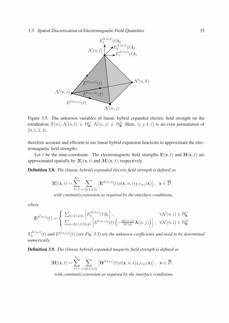
3.3. Spatial Discretization of Electromagnetic Field Quantities 35
EE(n,i,j)(t)
EE(n,i,k)(t)
EE(n,i,l)(t)
EN (n,l)1 (t)i1
EN (n,l)2 (t)i2
EN (n,l)3 (t)i3
N (n, i)
N (n, j)
N (n, k)
N (n, l)
Figure 3.5: The unknown variables of linear, hybrid expanded electric field strength on the
tetrahedron T (n), N (n, l) ∈ NCE, N (n, j) ∈ N
DE . Here, (i, j, k, l) is an even permutation of
(0, 1, 2, 3).
therefore accurate and efficient to use linear hybrid expansion functions to approximate the elec-
tromagnetic field strengths.
Let t be the time-coordinate. The electromagnetic field strengths E(x, t) and H(x, t) are
approximated spatially by [E](x, t) and [H](x, t), respectively.
Definition 3.8. The (linear, hybrid) expanded electric field strength is defined as
[E](x, t) =
NT∑
n=1
∑
i=0,1,2,3
[EN (n,i)(t)φ(x, n, i)χT (n)(x)
], x ∈ D,
with continuity extension as required by the interface conditions,
where
EN (n,i)(t) =
∑k=1,2,3
[E
N (n,i)k (t)ik
], ∀N (n, i) ∈ N
CE
∑j=0,1,2,3j/=i
[EE(n,i,j)(t)
(− |e(n,i,j)|
3V (n)A(n, j)
)], ∀N (n, i) ∈ N
DE
EN (n,i)k (t) and EE(n,i,j)(t) (see Fig. 3.5) are the unknown coefficients and need to be determined
numerically.
Definition 3.9. The (linear, hybrid) expanded magnetic field strength is defined as
[H](x, t) =
NT∑
t=1
∑
i=0,1,2,3
[HN (n,i)(t)φ(x, n, i)χT (n)(x)
], x ∈ D,
with continuity extension as required by the interface conditions,
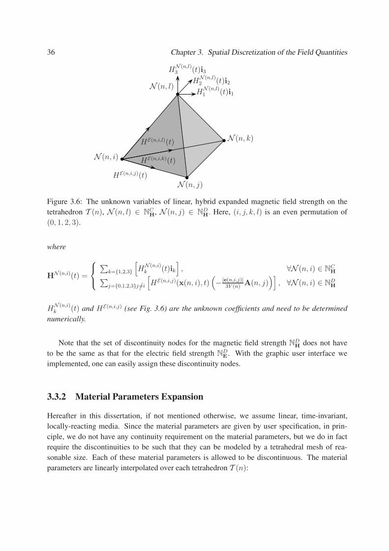
36 Chapter 3. Spatial Discretization of the Field Quantities
HE(n,i,j)(t)
HE(n,i,k)(t)
HE(n,i,l)(t)
HN (n,l)1 (t)i1
HN (n,l)2 (t)i2
HN (n,l)3 (t)i3
N (n, i)
N (n, j)
N (n, k)
N (n, l)
Figure 3.6: The unknown variables of linear, hybrid expanded magnetic field strength on the
tetrahedron T (n), N (n, l) ∈ NCH, N (n, j) ∈ N
DH. Here, (i, j, k, l) is an even permutation of
(0, 1, 2, 3).
where
HN (n,i)(t) =
∑k=1,2,3
[H
N (n,i)k (t)ik
], ∀N (n, i) ∈ N
CH
∑j=0,1,2,3j/=i
[HE(n,i,j)(x(n, i), t)
(− |e(n,i,j)|
3V (n)A(n, j)
)], ∀N (n, i) ∈ N
DH
HN (n,i)k (t) and HE(n,i,j) (see Fig. 3.6) are the unknown coefficients and need to be determined
numerically.
Note that the set of discontinuity nodes for the magnetic field strength NDH does not have
to be the same as that for the electric field strength NDE . With the graphic user interface we
implemented, one can easily assign these discontinuity nodes.
3.3.2 Material Parameters Expansion
Hereafter in this dissertation, if not mentioned otherwise, we assume linear, time-invariant,
locally-reacting media. Since the material parameters are given by user specification, in prin-
ciple, we do not have any continuity requirement on the material parameters, but we do in fact
require the discontinuities to be such that they can be modeled by a tetrahedral mesh of rea-
sonable size. Each of these material parameters is allowed to be discontinuous. The material
parameters are linearly interpolated over each tetrahedron T (n):

3.3. Spatial Discretization of Electromagnetic Field Quantities 37
• The globally expanded permeability function is
[µ](x) =
NT∑
n=1
∑
i=0,1,2,3
[µ(x(n, i))φ(x, n, i)χT (n)(x)
], x ∈ D,
with continuity extension as required. (3.19)
• The globally expanded permittivity function is
[ε](x) =
NT∑
n=1
∑
i=0,1,2,3
[ε(x(n, i))φ(x, n, i)χT (n)(x)
], x ∈ D,
with continuity extension as required. (3.20)
• The globally expanded electric conduction function is
[σ](x) =
NT∑
n=1
∑
i=0,1,2,3
[σ(x(n, i))φ(x, n, i)χT (n)(x)
], x ∈ D,
with continuity extension as required. (3.21)
• The globally expanded magnetic conduction function is
[κ](x) =
NT∑
n=1
∑
i=0,1,2,3
[κ(x(n, i))φ(x, n, i)χT (n)(x)
], x ∈ D,
with continuity extension as required. (3.22)
Note that, although the magnetic conductivity κ does not really exist in physics, we in-
troduce it here in order to apply Absorbing Boundary Conditions (ABC) with Perfectly
Matched Layers (PML).
For most cases, it is sufficient to assume the material parameters be constant within each element.
3.3.3 Electromagnetic Fluxes Interpolation
Throughout this thesis, we made the choice not to expand the magnetic flux densities B(x, t)
with face expansion functions (e.g. Whitney face expansion functions [14]), because we would
like to introduce an artificial magnetic conductivity κ(x) in order to apply absorbing boundary
conditions with Perfectly Matched Layers [12, 58]. With κ(x) being possibly discontinuous in
the domain of computation, both the tangential components and the normal components of the
magnetic flux density B(x, t) may be discontinuous across an interface of discontinuity. As for
the electric flux density D(x, t), both its tangential components and normal components can be

38 Chapter 3. Spatial Discretization of the Field Quantities
discontinuous when σ is discontinuous across the interface. It is the total current density that
exhibits continuity in the normal components (Section 2.1.4).
A fully consistent interpolation scheme requires the total current electric density and total
magnetic current density to be interpolated with consistently linear face expansion functions.
This introduces many more unknown coefficients along with many more equations as shown in
[26]. In Section 5.2, we test the SIFE method with the same test configurations as those in [26]
and we show that the SIFE method is able to obtain better accuracy with less computational
costs. Considering all these, we chose to represent the expanded electromagnetic fluxes with
the expanded electromagnetic field strengths and the constitutive relations and we claim that this
choice boosts efficiency without compromising the underlying physics.
• The globally expanded electric flux densities are:
[D](x, t) =
NT∑
n=1
∑
i=0,1,2,3
[ε(x(n, i))EN (n,i)(t)φ(x, n, i)χT (n)(x)
], x ∈ D,
with continuity extension as required by the interface conditions. (3.23)
• The globally expanded magnetic flux densities are:
[B](x, t) =
NT∑
n=1
∑
i=0,1,2,3
[µ(x(n, i))HN (n,i)(t)φ(x, n, i)χT (n)(x)
], x ∈ D,
with continuity extension as required by the interface conditions. (3.24)
3.3.4 Conduction Current Densities Interpolation
Out of similar considerations as those in Section 3.3.3, we choose not to interpolate the Conduc-
tion Electromagnetic Current densitiesK(x, t) and J(x, t) with additional unknown coefficients.
Instead we discretize the current densities with the expanded electromagnetic field strengths and
the constitutive relations.
• The expanded conducted electric current densities are:
[J](x, t) =
NT∑
n=1
∑
i=0,1,2,3
[σ(x(n, i))EN (n,i)(t)φ(x, n, i)χT (n)(x)
],x ∈ D,
with continuity extension as required. (3.25)
• The expanded conducted magnetic current densities are:
[K](x, t) =
NT∑
n=1
∑
i=0,1,2,3
[κ(x(n, i))HN (n,i)(t)φ(x, n, i)χT (n)(x)
], x ∈ D,
with continuity extension as required. (3.26)
3.4. Discussion 39
3.3.5 Volume Charge Density Expansion
We do not have any continuity requirement on the volume density of the electric charge since it
is given as an input function. The volume density of electric charge is linearly interpolated over
each tetrahedron T (n):
[ρ](x) =
NT∑
n=1
∑
i=0,1,2,3
[ρ(x(n, i))φ(x, n, i)χT (n)(x)
], x ∈ D,
with continuity extension as required. (3.27)
3.3.6 Impressed Electric Current Expansion
We do not have any continuity requirement on the volume density of impressed current. If neces-
sary and physically correct, all components of the current density are allowed to be discontinuous
across the interfaces. The known impressed current densities are linearly interpolated over each
tetrahedron T (n):
[JimpT (n)](x, t) =
∑
i=0,1,2,3
[Jimp(x(n, i), t)φ(x, n, i)
]. (3.28)
The globally expanded functions of the impressed current densities are:
[Jimp](x, t) =
NT∑
n=1
∑
i=0,1,2,3
[Jimp(x(n, i), t)φ(x, n, i)χT (n)(x)
], x ∈ D,
with continuity extension as required. (3.29)
In the SIFE method, we can apply the exact current source if the exact electric current passing
through each facet in the mesh can be obtained, due to the fact that the current densities are
always integrated on faces. However, the source currents will be computed approximately by the
trapezoidal rule in space when the exact integrals are not available.
3.4 Discussion
Due to the interface conditions, a straightforward application of linear expansion functions would
lead to large numerical error or excessive mesh refinement. Applying these interfaces conditions
as constraints with Lagrange multipliers results in semi-positive definite system matrices which
are difficult to solve (see [33, 32]). It is advantageous to take them into account when discretizing
the field quantities. Therefore, in this chapter, we have introduced another important ingredient
(the spatial discretization scheme) to the SIFE method, the first ingredient being the surface
integrated field equations.

40 Chapter 3. Spatial Discretization of the Field Quantities
Compared to the edge element first suggested by Bossavit, (1) this spatial discretization
scheme is complete to the first order and second-order accurate. (2) Such a spatial discretiza-
tion scheme can handle complicated cases that are not divergence-free. (3) The new discretiza-
tion scheme combines the use of nodal elements and consistently linear edge elements. Thus it
achieves second-order accuracy with low computational cost. (4) It interpolates simultaneously
both field strengths and delivers the same order of accuracy for both electric and magnetic field
strengths.
In the following chapter, we will use this scheme to discretize the field quantities in the
surface integrated field equations presented before, and formulate the discrete equations that are
to be solved for the computation of the electromagnetic field.

Chapter 4
The Surface Integrated Field Equations Method
Law of Conservation of Perversity: we can’t make something
simpler without making something else more complex.
Norberto Meijome
In this chapter, we introduce the Surface Integrated Field Equationsmethod (the SIFEmethod)
which applies the surface integrated Maxwell equations. With the linear expansion functions in-
troduced in the last chapter, this method constructs systems of linear equations for computing
static and stationary electric and magnetic fields as well as electromagnetic waves in both the
frequency and time domain.
4.1 Static and Stationary Electric and Magnetic Fields
In this section, we replace the continuous field quantities in the generic surface integrated field
equations for static and stationary electric and magnetic fields, presented in Sec. 2.3, with its
discrete linear counterparts to derive a system of linear, algebraic equations in terms of unknown
coefficients (degrees of freedom). By solving the system of linear equations, we obtain an ap-
proximated field in the domain of computation.
In the SIFE method for computing static and stationary electric and magnetic fields, we want
the linearly interpolated field quantities to satisfy Eq. (2.23) and Eq. (2.26) at the bounding sur-
faces of each elemental volume. Moreover, the interpolated field must comply with the interface
conditions Eqs. (2.28) - (2.29) and boundary conditions Eqs. (2.30), (2.31).
4.1.1 Discrete Surface Integrated Curl-Equation
Let V(x) denote a generic field strength as shown in Section 2.3, applying Eq. (2.23) on every
facet of every tetrahedron, F(n, i); n ∈ IT , i = 0, 1, 2, 3, we have∮
∂F(n,i)
V(x) · dl =
∫
F(n,i)
Qimp(x) · dA, for n ∈ IT , i ∈ 0, 1, 2, 3. (4.1)
The impressed (known) current source Qimp(x) is assumed to be divergence free. The total
number of above equations that we can formulate equals the total number of facets in the trian-
gulation.
41

42 Chapter 4. The Surface Integrated Field Equations Method
N (n, i)
N (n, j)
N (n, k)
N (n, l)
V1E(n,l,j)
V1E(n,j,k)
V1E(n,k,l) Q2
F(n,i)
Figure 4.1: The Curl-equations integrated over the facet F(n, i).
Let the face F(n, i) be delimited by the nodesN (n, j),N (n, k) andN (n, l) where (i, j, k, l)
is an even permutation of (0, 1, 2, 3). We can rewrite Eq. (4.1) as:
∫
E(n,j,k)
V(x) · dl +∫
E(n,k,l)
V(x) · dl +∫
E(n,l,j)
V(x) · dl =
∫
F(n,i)
Qimp(x) · dA. (4.2)
Definition 4.1. Let V1E(n,i,j) denote the line integrals of V(x) along the edge E(n, i, j); n ∈ IT ,
i, j ∈ 0, 1, 2, 3,i/=j , i.e.
V1E(n,i,j) =
∫
E(n,i,j)
V(x) · dl.
Its discrete counterpart is denoted as [V]1E(n,i,j).
Note that:
V1E(n,i,j) = −V1
E(n,j,i), [V]1E(n,i,j) = −[V]1E(n,j,i).
Definition 4.2. Let Q2F(n,i) be the integral of Q
imp(x) on the two dimensional manifold
F(n, i); n ∈ IT , i = 0, 1, 2, 3, i.e.
Q2F(n,i) =
∫
F(n,i)
Qimp(x) · dA.
Its discrete counterpart is denoted as [Q]2F(n,i).
With Def. 4.1 and Def. 4.2, we can write Eq. (4.2) as
V1E(n,j,k) + V1
E(n,k,l) + V1E(n,l,j) = Q2
F(n,i),
for n ∈ IT ; (i, j, k, l) is an even permutation of (0, 1, 2, 3), (4.3)

4.1. Static and Stationary Electric and Magnetic Fields 43
as shown in Fig. (4.1).
With the absence of a current source on the interfaces, i.e. QimpS (x) = 0, x ∈ I, the
field strength V(x) has continuous tangential component across the interfaces of discontinuity.
Therefore we may approximate the field strength with linear hybrid expansion functions as in
Section 3.3.1, and the impressed current source with linear expansion functions as in Section
3.3.6. Furthermore, we define
Definition 4.3. For n ∈ IT and i ∈ 0, 1, 2, 3,
VN (n,i) =
∑k=1,2,3
[V
N (n,i)k ik
], ∀N (n, i) ∈ N
CV
∑j=0,1,2,3j/=i
[V E(n,i,j)
(− |e(n,i,j)|
3V (n)A(n, j)
)], ∀N (n, i) ∈ N
DV
where VN (n,i)k and V E(n,i,j) are the linear expansion coefficients (degrees of freedom) which are
to be determined numerically.
With the properties of φ(x, n, i) presented in Section 3.2.1, we find that the line integral of
the field strength is actually approximated by the trapezoidal rule, i.e.
[V]1E(n,j,k) =1
2e(n, j, k) ·
[VN (n,j) + VN (n,k)
],
for n ∈ IT , j, k ∈ 0, 1, 2, 3, j /=k. (4.4)
The surface integral of the impressed current density is also approximated by the trapezoidal
rule:
[Q]2F(n,i) =1
3A(n, i) ·
[∑
h=j,k,l
Qimp(x(n, h))
],
for n ∈ IT ; (i, j, k, l) is an even permutation of (0, 1, 2, 3). (4.5)
Finally, substituting Eq. (4.4) and Eq. (4.5) into the discrete surface integrated equation for static
and stationary fields, i.e.
[V]1E(n,j,k) + [V]1E(n,k,l) + [V]1E(n,l,j) = [Q]2F(n,i),
for n ∈ IT ; (i, j, k, l) is an even permutation of (0, 1, 2, 3), (4.6)
we obtain the linear equations:
1
2e(n, j, k) ·
[VN (n,j) + VN (n,k)
]+
1
2e(n, k, l) ·
[VN (n,k) + VN (n,l)
]
+1
2e(n, l, j) ·
[VN (n,l) + VN (n,j)
]=
1
3A(n, i) ·
[∑
h=j,k,l
Qimp(x(n, h))
],
for n ∈ IT ; (i, j, k, l) is an even permutation of (0, 1, 2, 3).

44 Chapter 4. The Surface Integrated Field Equations Method
N (n, i)
N (n, j)
N (n, k)
N (n, l)
F2F(n,i)
F2F(n,k)
F2F(n,l)
F2F(n,j)
Figure 4.2: Equation (2.26) applied to the bounding surface of the tetrahedron T (n).
With simple vector calculus, we simplify the above equation as:
1
2e(n, l, k) · VN (n,j) +
1
2e(n, j, l) · VN (n,k) +
1
2e(n, k, j) ·VN (n,l)
=∑
h=j,k,l
[1
3A(n, i) · Qimp(x(n, h))
],
for n ∈ IT ; (i, j, k, l) is an even permutation of (0, 1, 2, 3), (4.7)
where VN (n,i) is defined in Def. 4.3.
4.1.2 Discrete Surface Integrated Compatibility Equation
Let F(x) be a symbol to represent any generic flux density. Applying Eq. (2.26) on the bounding
surface ∂T (n); n ∈ IT of every tetrahedron T (n); n ∈ IT , we have∮
∂T (n)
F(x) · dA =
∫
T (n)
ρimp(x)dV, for n ∈ IT . (4.8)
The total number of such independent equations is equal to the total number of tetrahedrons in
the triangulation. Eq. (4.8) can also be written as:
3∑
i=0
[∫
F(n,i)
F(x) · dA]
=
∫
T (n)
ρimp(x)dV, for n ∈ IT . (4.9)
Definition 4.4. Let F2F(n,i); n ∈ IT , i = 0, 1, 2, 3 be the surface integral of F(x) over the
two-dimensional manifolds F(n, i); n ∈ IT , i = 0, 1, 2, 3, i.e.
F2F(n,i) =
∫
F(n,i)
F(x) · dA.
Its discrete counterpart is denoted as [F]2F(n,i).

4.1. Static and Stationary Electric and Magnetic Fields 45
Definition 4.5. Let ρ3T (n); n ∈ IT , i = 0, 1, 2, 3 be the volume integral of ρimp(x) over the
three-dimensional manifolds T (n); n ∈ IT , i = 0, 1, 2, 3, i.e.
ρ3T (n) =
∫
T (n)
ρimp(x)dV.
Its discrete counterpart is denoted as [ρ]3T (n).
With Def. 4.4 and Def. 4.5, we rewrite Eq. (4.9) as (see Fig. 4.2)
3∑
i=0
F2F(n,i) = ρ3
T (n), for n ∈ IT . (4.10)
With the flux densities linearly interpolated as mentioned in Section 3.3.3, the surface integrals
are actually approximated by the trapezoidal rule:
[F]2F(n,i) =
∫
F(n,i)
[F](x) · dA =∑
h=j,k,l
[1
3A(n, i) · ξ(x(n, h))VN (n,h)
],
for n ∈ IT ; (i, j, k, l) is an even permutation of (0, 1, 2, 3). (4.11)
VN (n,k) is defined in Definition 4.3. The volume integral of ρ(x) is approximated by:
[ρ]3T (n) =∑
h=i,j,k,l
[1
4V (n)ρimp(x(n, h))
],
for n ∈ IT ; (i, j, k, l) is an even permutation of (0, 1, 2, 3). (4.12)
Substituting Eq. (4.11) and Eq. (4.12) into the discrete surface integrated field equation for
generic fields, i.e.
3∑
i=0
[F]2F(n,i) = [ρ]3T (n), for n ∈ IT , (4.13)
we obtain:
−∑
h=i,j,k,l
[1
3A(n, h) · ξ(x(n, h))VN (n,h)
]=
∑
h=i,j,k,l
[1
4V (n)ρimp(x(n, h))
],
for n ∈ IT ; (i, j, k, l) is an even permutation of (0, 1, 2, 3), (4.14)
where VN (n,k) is defined in Def. 4.3; VN (n,i)k and V E(n,i,j) are the unknown variables in these
linear equations.

46 Chapter 4. The Surface Integrated Field Equations Method
N (n1, i1)
N (n1, j1)
N (n1, k1)
N (n1, l1) N (n2, i2)
N (n2, j2)
N (n2, k2)
N (n1, l1)N (m)
N (u)
N (l)
Figure 4.3: The two tetrahedrons T (n1) and T (n2) share one facet on the interface. We have
n1, n2 ∈ IT and m, u, l ∈ IN . Here, (i1,j1,k1,l1) and (i2,j2,k2,l2) are both even permuta-
tions of (0, 1, 2, 3). For clarity, we pulled the two tetrahedrons a little bit away from the in-
terface. N (n1, j1), N (u),N (n2, k2), N (n1, k1), N (l), N (n2, j2) and N (n1, l1), N (m),
N (n2, l2), respectively, represent the same node.
4.1.3 Discrete Interface Conditions
As we have mentioned, the interface conditions must be satisfied for the solutions to be unique
and well defined. Since we use linear hybrid expansion functions to interpolate field strengths,
the tangential components of the approximated field strength across the interface of discontinu-
ity are continuous, i.e. Eq. (2.28) is automatically satisfied when there is no surface current.
However, the discretization scheme will not satisfy the continuity requirement for the normal
components of fluxes across interfaces of discontinuity, i.e. Eq.(2.29) if additional constraints
are not taken into account. Therefore, we need to discretize and explicitly enforce normal con-
tinuity of the fluxes. To be consistent with our surface integrated field equations scheme and
to reduce the number of additional equations that we shall introduce, we choose to work with
surface integrated interface conditions, that is, let T (n1) and T (n2) be two tetrahedrons sharing
one face which is locally labeled as F(n1, i1) in T (n1) and F(n2, i2) in T (n2) as indicated in
Fig. 4.3, one or more nodes delimiting this face locate on the interfaces of discontinuity. Inte-
grating Eq.(2.29) over the face F(n1, i2), we have
∫
F(n1,i1)
F(x) · dA +
∫
F(n2,i2)
F(x) · dA =
∫
F(n2,i2)
σimp(x)dA (4.15)
or equivalently:
F2
F(n1,i1)+ F2
F(n2,i2)= σ2
F(n2,i2), (4.16)
where:

4.1. Static and Stationary Electric and Magnetic Fields 47
F2F(n1,i1)
F2F(n2,i2)
N (n1, i1)N (n2, i2)
Figure 4.4: The two tetrahedra T (n1) and T (n2) share one facet on the interface. We have
n1, n2 ∈ IT , and F2
F(n1,i1)and F2
F(n2,i2)are taken in opposite direction.
• n1, n2 ∈ IT , n1/=n2.
• T (n1) and T (n2) share the same face locally labeled as F(n1, i1) in T (n1) and F(n2, i2)
in T (n2).
• Here, (i1,j1,k1,l1) and (i2,j2,k2,l2) are both even permutations of (0, 1, 2, 3).
• There exists j ∈ j1,k1,l1 such thatN (n1, j) ∈ NDV.
Note that a “plus” sign is taken in the above equation. This is because the normal directions of
F(n1, i1) and F(n2, i2) are taken opposite to each other as indicated in Fig. (4.4). Substituting
Eq. (4.11) in the discrete surface integrated interface condition, i.e.
[F]2F(n1,i1)
+ [F]2F(n2,i2)
= [σ]2F(n1,i1)
, (4.17)
we obtain:
∑
j=j1,k1,l1
[1
3A(n1, i1) · ξ(x(n1, j))VN (n1,j)
]
+∑
j=j2,k2,l2
[1
3A(n2, i2) · ξ(x(n2, j))VN (n2,j)
]
=∑
j=j1,k1,l1
[1
3A(n1, i1)σimp(x(n1, j))
], (4.18)
where:
• n1, n2 ∈ IT , T (n1) ∈ T and T (n2) ∈ T , n1/=n2.
48 Chapter 4. The Surface Integrated Field Equations Method
• T (n1) and T (n2) share the same face locally labeled as F(n1, i1) in T (n1) and F(n2, i2)
in T (n2).
• Here, (i1,j1,k1,l1) and (i2,j2,k2,l2) are both even permutations of (0, 1, 2, 3).
• There exists j ∈ j1,k1,l1 such thatN (n1, j) ∈ NDV.
Similar to the other discrete surface integrated equations,VN (n,k); n ∈ IT , k = 0, 1, 2, 3
is
defined in Def. 4.3 andV
N (n,i)k ; n ∈ IT , i = 0, 1, 2, 3,N (n, i) ∈ N
CV, k = 1, 2, 3
and
V E(n,i,j); n ∈ IT , i, j = 0, 1, 2, 3,N (n, i) ∈ NDV, j /=i are the unknown variables in these linear
equations.
4.1.4 Discrete Boundary Conditions
For simplicity, we choose to implement the boundary conditions Eq. (2.30) and Eq.(2.31) as
additional equations of constaints on each node of the boundary. Let ∂D be the boundary of the
computational domain D. For static and stationary problems, we have two types of boundary
conditions:
• Prescribed tangential field component boundary conditions
ν × V(x) = ν ×Vext(x), x ∈ ∂DV. (4.19)
• Prescribed normal flux component boundary conditions.
ν · V(x) = ν · Vext(x), x ∈ ∂DF, (4.20)
where ∂DV⋃
∂DF = ∂D, ∂DV⋂
∂DF = ∅. Replacing the continuous field strengths on
the boundary with their discrete counterparts and applying the discrete boundary condition on
boundary nodes, we obtain (in vector notation):
• Discrete, prescribed tangential field component boundary conditions
ν × VN (n,i) = ν × VN (n,i),ext, x(n, i) ∈ ∂DV. (4.21)
• Discrete, prescribed normal flux component boundary conditions.
ν ·VN (n,i) = ν · VN (n,i),ext, x(n, i) ∈ ∂DF. (4.22)
VN (n,i) is defined in Definition 4.3.

4.1. Static and Stationary Electric and Magnetic Fields 49
4.1.5 Total Number of Equations vs. Total Number of Unknowns
As we formulate the system with Eqs. (4.7), (4.14), (4.18), and the discrete boundary conditions
Eq. (4.21) and Eq. (4.22), we would like to make sure that we have enough equations to determine
all the unknown coefficients.
For simplicity and clarity, we adopt in this section a notation that differs from previous sec-
tions especially in the meaning of the symbol ‘N’ which here indicates the multiplicity of a
certain object.
Let F denote the total number of facets in the mesh, and Fb denote the total number of facets
on the boundary. The total number of the discrete equations Eq. (4.7) that we can formulate is
Neq1 = F − Fb. (4.23)
Assuming Qimp(x) is divergence free, it is evident that for each element, one of these equations
is a linear combination of the other equations. Therefore, let T denote the total number of
elements in the mesh, then the total number of linearly independent Eqs. (4.7) we can formulate
is:
Neq1 = F − Fb − T. (4.24)
The total number of the discrete equations due to Eq. (4.14) is:
Neq2 = T. (4.25)
The total number of discrete interface conditions due to Eq. (4.18) is
Nint = Fint, (4.26)
where Fint is the total number of the facets that are delimited by at least one discontinuity node.
Let V denote the total number of nodes in the mesh, VC the total number of continuity nodes
and VD the total number of discontinuity nodes, respectively. Let Eb denote the total number
of edges on the boundary. When Dirichlet boundary conditions are used, the total number of
unknowns (DOF) in the domain is
Nun = 3VC + xVD − 2Eb, (4.27)
where x is the average number of edges emerging from each discontinuity node and V = VC +
VD. Here we assume that discontinuity nodes are used on the boundary of the computational
domain.
Let Neq = Neq1 + Neq2 + Nint be the total number of independent linear equations in the
system, we have
Neq − Nun = Neq1 + Neq2 + Nint − Nun
= F + 2Eb − Fb − 3V + Fint − (x − 3)VD. (4.28)

50 Chapter 4. The Surface Integrated Field Equations Method
Euler’s formula for two dimensional objects applied to the boundary gives
Fb + Vb − Eb = χ, (4.29)
where χ is the Euler characteristic of which the value is normally ‘2’ and very small when
compared to other values. With the above formula, we can write
Neq − Nun = F + Eb + Vb − χ − 3V + Fint − (x − 3)VD. (4.30)
Although a more elaborated analysis can be carried out, it is sufficient to just consider two ex-
treme cases.
1. If the whole domain consists of continuity nodes, that is, VD = 0, Fint = 0, we have
Neq − Nun = F + Eb + Vb − χ − 3V. (4.31)
As long as the total number of facets is more than three times the total number of nodes, the
system is guaranteed to be overdetermined. This condition is easily satisfied by tetrahedral
meshes or hexahedral meshes.
2. If the whole domain consists of discontinuity nodes, that is, VD = V , Fint = F and
xVD = 2E, we have
Neq − Nun = 2F + Eb + Vb − χ − 2E. (4.32)
As long as the total number of facets is greater than the total number of edges, the system
is guaranteed to be overdetermined. This condition is again easily satisfied by tetrahedral
meshes and hexahedral meshes.
In conclusion, we obtain a system of linear equations with more independent linear equations
than the unknown coefficients. Then, we seek a least-squares solution to the over-determined
system.
4.1.6 Building the Linear System with the Least-Squares Method
With Eqs. (4.7), (4.14), (4.18), and the discrete boundary conditions Eqs. (4.21) and (4.22), we
have a system of linear equations with more equations that unknown coefficients (as it is shown
in Section 4.1.5) with respect to the unknown variables V N (n,i)k ; n ∈ IT , i = 0, 1, 2, 3,N (n, i) ∈
NCV, k = 1, 2, 3 and V E(n,i,j); n ∈ IT , i, j = 0, 1, 2, 3,N (n, i) ∈ N
DV, j /=i. Assuming that we
have l equations with respect to m unknown variables, collecting all unknown variables into a
column vector u and coefficients into a system matrix K, we have:
k11 k12 · · · k1m
k21 k22 · · · k2m
......
. . ....
kl1 kl2 · · · klm
u1
u2
...
um
=
f1
f2
...
fl
(4.33)

4.1. Static and Stationary Electric and Magnetic Fields 51
or simply
Ku = f . (4.34)
Such an over-determined system may have no solution at all. One thing that we can do is to
find an approximated solution which minimizes a certain quadratic functional. The (weighted)
least-squares method amounts to minimize the following summation of the weighted squared
residuals:
I(u) =
l∑
i=1
wi(
m∑
j=1
kijuj − fi)2, (4.35)
where wi ≥ 0; i = 1, · · · , l are the weighting factors of each equation. Note that, if wj = 0,
the jth equation is effectively ignored. The minimizer of I(u) is the solution of the normal
equation:
KTWKu = KTWf , where W = diag(w1, w2, · · · , wl). (4.36)
Using a local assembly procedure [60], we can easily construct this normal equation, which we
then solve with a preconditioned iterative linear solution method. Since the over-determined
system is very sparse, the system of the normal equation is sparse as well.
Note that if any of the discrete boundary condition equations ends up involving only one
unknown coefficient, e.g. VN (n,i)3 = 0, then this boundary condition equation can be applied
exactly, e.g. by eliminating the corresponding rows and columns [31], by explicitly eliminating
the known variables [60], or by assigning a very big (e.g. 1020) diagonal entry in the system
matrix for the corresponding coefficient [31]; otherwise, the boundary conditions will be satisfied
in least-squares sense. However, one can increase its corresponding weighting factor such that
the approximated solution will satisfy the constraint better.
After solving the system for the coefficients, we get an approximated field strength in the
domain of computation. One might think that by taking the normal equations, the condition
number of the resulting system matrix is squared and the number of iterations needed to reach
convergence should be a lot, however, as we will show in Section 5.1 that the convergence of the
least-squares SIFE method is not too bad at all. In fact, it is even more efficient than a traditional
Galerkin method.
4.1.7 Normalization of the Linear System
Due to the fact that computer numbers have finite precision, the system matrix must have a rea-
sonable condition number for the linear solver to deliver an accurate solution, otherwise, it would
take too much time for the iterative linear solvers to converge or the computed solution would not
make any sense. Huge jumps in the magnitudes of the variables should be avoided. Therefore,

52 Chapter 4. The Surface Integrated Field Equations Method
in the numerical computations, we need to normalize the field quantities such that no extreme
numbers will show up. Different field normalization schemes can be used. Throughout this the-
sis, we choose the scheme presented by Remis in [11]. However, in order to handle extreme
contrasts in the material parameters, we also have to normalize the equations with weighting
factors wi ≥ 0; i = 1, · · · , l. Note that if we use the least-squares method to find the approxi-
mated solution, the solution only makes sense if Eqs. (4.7), (4.14) and (4.18) are equally treated
and respected. The problem is that a material parameter can be as big as 103 or even more (see
Section 5.1.2), and Eq. (4.14) has the material parameter ξ in its coefficients, while Eq. (4.7)
does not. This problem affects the solution unless the system is square, in which case the system
shall most likely have a very bad condition number. To treat these equations fairly and improve
the condition number of the linear system, we propose to weight Eq. (4.14) with the inverse of
the average relative ξ(x) in the tetrahedron. This helps in handling cases with extremely high
contrasts (see Section 5.1.2).
4.2 Electromagnetic Problems in the Frequency Domain
In this section, the continuous field quantities in the frequency-domain surface integratedMaxwell
equations (Section 2.2) are replaced with their discrete linear counterparts to derive a system
of linear, complex, algebraic equations in terms of unknown coefficients (degrees of freedom).
Here, we assume that the media present in the configurations are linear, instantaneously locally
reacting, and possibly inhomogeneous. We study the compatibility equations and interface con-
ditions in the integral form. The derived scheme complies with the compatibility equations and
interface equations automatically.
4.2.1 Normalization of the Field Quantities
Before formulating the system of equations, it is important to normalize the equations so that the
magnitude of significant coefficients in the equations is more or less comparable. In this way,
the system has better spectral properties. Let L be a problem related reference length, e.g. the
diameter of the computational domain. We normalize the spatial coordinate, angular frequency,
field quantities, EM sources and material parameters as follows:
x =x
L, ω =
Lω
c0, E(x, ω) = E(x, ω),
H(x, ω) =
õ0
ε0
H(x, ω), Jimp(x, ω) = L
õ0
ε0
Jimp(x, ω),
σ(x) = L
õ0
ε0σ(x), ε(x) = ε(x), µ(x) = µ(x),
B(x, ω) =1
µ0
B(x, ω), D(x, ω) =1
ε0
D(x, ω), (4.37)

4.2. Electromagnetic Problems in the Frequency Domain 53
where the symbols with a hat denote the normalized field quantities, µ0 denotes the permeability
in vacuum, ε0 the permittivity in vacuum and c0 the speed of light in vacuum, respectively. The
normalized field quantities obviously satisfy the normalized Maxwell’s equations. For clarity,
hereafter in this section, we will drop the hats in formulating the discrete system. But the nor-
malized field quantities and normalized Maxwell equations are used. As soon as approximate
solutions to the normalized equations have been found, we can convert to the un-normalized
quantities using Eq. (4.37).
4.2.2 Discrete Ampere’s Equation in the Frequency Domain
Applying Ampere’s equation (2.15) on every facet F(n, i); n ∈ IT , i = 0, 1, 2, 3 of every tetra-hedron T (n); n ∈ IT , we have
∮
∂F(n,i)
H(x, ω) · dl− jω
∫
F(n,i)
D(x, ω) · dA −∫
F(n,i)
Jtot(x, ω) · dA = 0. (4.38)
Let the facet F(n, i) be delimited by N (n, j),N (n, k),N (n, l), where (i, j, k, l) is an even per-
mutation of (0, 1, 2, 3). We can write the first term of the above equation as:∮
∂F(n,i)
H(x, ω) · dl =
∫
E(n,j,k)
H(x, ω) · dl +∫
E(n,k,l)
H(x, ω) · dl +∫
E(n,l,j)
H(x, ω) · dl. (4.39)
Definition 4.6. We denote the line integral of H(x, ω) on the one-dimensional manifold
E(n, i, j), ω; n ∈ IT , i, j = 0, 1, 2, 3, i/=j by H1E(n,i,j),ω, i.e.
H1E(n,i,j),ω =
∫
E(n,j,k)
H(x, ω) · dl.
We denote its approximated counterpart as [H]1E(n,i,j),ω.
Note that:
H1E(n,i,j),ω = −H1
E(n,j,i),ω, [H]1E(n,i,j),ω = −[H]1E(n,j,i),ω. (4.40)
Then: ∫
∂F(n,i)
H(x, ω) · dl = H1E(n,j,k),ω + H1
E(n,k,l),ω + H1E(n,l,j),ω.
Assuming the interfaces are free of current sources, the electromagnetic field strengths H(x, ω)
and E(x, ω) have continuous tangential component across the interfaces of discontinuity. There-
fore we may approximate the field strengths with linear hybrid expansion functions presented in
Section 3.3.1. For the line integrals we get
[H]1E(n,j,k) =1
2e(n, j, k) · [HN (n,j)(ω) + HN (n,k)(ω)], (4.41)

54 Chapter 4. The Surface Integrated Field Equations Method
where HN (n,j)(ω) is defined as follows
Definition 4.7. For n ∈ IT and i ∈ 0, 1, 2, 3, we have
HN (n,i)(ω) =
∑k=1,2,3
[H
N (n,i)k (ω)ik
], ∀N (n, i) ∈ N
CH
∑j=0,1,2,3j/=i
[HE(n,i,j)(ω)
(− |e(n,i,j)|
3V (n)A(n, j)
)], ∀N (n, i) ∈ N
DH
HN (n,i)k (ω) and HE(n,i,j)(ω) are the unknown coefficients, which are also known as degrees of
freedom (DOF) or Unknowns.
The remaining terms of Eq. (4.38) can be written as:∫
F(n,i)
[Jimp(x, ω) + J(x, ω) + jωD(x, ω)
]· dA. (4.42)
Now let Jtot2F(n,i),ω be the surface integral of Jtot(x, ω) on the two-dimensional manifoldF(n, i), ω,
Jtot2F(n,i),ω =
∫
F(n,i)
Jtot(x, ω) · dA.
Let Jimp2F(n,i),ω be the surface integral of Jimp(x, ω) on the two-dimensional manifoldF(n, i), ω,
Jimp2F(n,i),ω =
∫
F(n,i)
Jimp(x, ω) · dA.
Let J2F(n,i),ω be the surface integral of J(x, ω) on the two-dimensional manifold F(n, i), ω,
J2F(n,i),ω =
∫
F(n,i)
J(x, ω) · dA.
Let D2F(n,i),ω be the surface integral of D(x, ω) on the two-dimensional manifold F(n, i), ω, that
is,
D2F(n,i),ω =
∫
F(n,i)
D(x, ω) · dA.
We can then rewrite Eq. (4.42) as
Jimp2F(n,i),ω + J2
F(n,i),ω + jωD2F(n,i),ω. (4.43)
With Jimp(x, ω) being spatially interpolated as shown in Section 3.3.6, we compute the approx-
imated surface integrals by the trapezoidal rule. This gives
[Jimp]2F(n,i),ω =1
3A(n, i) ·
∑
h=j,k,l
Jimp(x(n, h), ω). (4.44)
With J(x, ω) being spatially interpolated as shown in Section 3.3.4 and made explicit in the
following definition:

4.2. Electromagnetic Problems in the Frequency Domain 55
Definition 4.8. For n ∈ IT and i ∈ 0, 1, 2, 3:
EN (n,i)(ω) =
∑k=1,2,3
[E
N (n,i)k (ω)ik
], ∀N (n, i) ∈ N
CE
∑j=0,1,2,3j/=i
[EE(n,i,j)(ω)
(− |e(n,i,j)|
3V (n)A(n, j)
)], ∀N (n, i) ∈ N
DE
EN (n,i)k (ω) and EE(n,i,j)(ω) are the unknown coefficients, which are also known as degrees of
freedom (DOF) or unknowns.
We compute the approximated surface integrals by the trapezoidal rule. This gives
[J]2F(n,i),ω =1
3A(n, i) ·
∑
h=j,k,l
[σ(x(n, h))EN (n,h)(ω)
]. (4.45)
With D(x, ω) being spatially interpolated as shown in Section 3.3.3, we compute the approxi-
mated surface integrals for the electric fluxes by the trapezoidal rule as well. We obtain
[D]2F(n,i),ω =1
3A(n, i) ·
∑
h=j,k,l
[ε(x(n, h))EN (n,h)(ω)
], (4.46)
where EN (n,j)(ω); n ∈ IT , j = 0, 1, 2, 3 is defined in Def. 4.8.
Substituting Eqs. (4.41), (4.46), (4.45) and (4.44) in the discrete surface integrated Ampere’s
equation in the frequency domain, i.e.
[H]1E(n,j,k),ω + [H]1E(n,k,l),ω + [H]1E(n,l,j),ω = [Jimp]2F(n,i),ω + [J]2F(n,i),ω + jω[D]2F(n,i),ω, (4.47)
and by moving all known terms to the right-hand-side, we arrive at
1
2e(n, l, k) · HN (n,j)(ω) +
1
2e(n, j, l) · HN (n,k)(ω) +
1
2e(n, k, j) · HN (n,l)(ω)
−∑
h=j,k,l
1
3A(n, i) [σ(x(n, h)) + jωε(x(n, h))] ·EN (n,h)(ω)
=∑
h=j,k,l
[1
3A(n, i) · Jimp(x(n, h), ω)
], (4.48)
where
• n ∈ IT , (i, j, k, l) is an even permutation of (0, 1, 2, 3).
• HN (n,j)(ω); j = 0, 1, 2, 3 is defined in Def. 4.7.
• EN (n,j)(ω); j = 0, 1, 2, 3 is defined in Def. 4.8.
• HN (n,i)k (ω); n ∈ IT , i = 0, 1, 2, 3, N (n, i) ∈ N
CH, k = 1, 2, 3 and HE(n,i,j)(ω); n ∈
IT , i, j = 0, 1, 2, 3, N (n, i) ∈ NDH, j /=i, EN (n,i)
k (ω); n ∈ IT , i = 0, 1, 2, 3, N (n, i) ∈N
CE, k = 1, 2, 3 and EE(n,i,j)(ω); n ∈ IT , i, j = 0, 1, 2, 3, N (n, i) ∈ N
DE , j /=i are the
unknown coefficients.

56 Chapter 4. The Surface Integrated Field Equations Method
4.2.3 Discrete Faraday’s Equation in the Frequency Domain
Applying Faraday’s equation (2.16) on every facet F(n, i); n ∈ IT , i = 0, 1, 2, 3 of every tetra-hedron T (n); n ∈ IT , we have
∮
∂F(n,i)
E(x, ω) · dl + jω
∫
F(n,i)
B(x, ω) · dA = 0. (4.49)
With a similar procedure presented in Section 4.2.2, we may discretize the above equation and
obtain the following discrete surface integrated Faraday equations in the frequency domain:
1
2e(n, l, k) · EN (n,j)(ω) +
1
2e(n, j, l) · EN (n,k)(ω) +
1
2e(n, k, j) · EN (n,l)(ω)
+jω∑
h=j,k,l
1
3A(n, i) · µ(x(n, h))HN (n,h)(ω) = 0, (4.50)
where
• n ∈ IT , (i, j, k, l) is an even permutation of (0, 1, 2, 3).
• HN (n,j)(ω); j = 0, 1, 2, 3 is defined by Def. 4.7.
• EN (n,j)(ω); j = 0, 1, 2, 3 is defined by Def. 4.8.
• HN (n,i)k (ω); n ∈ IT , i = 0, 1, 2, 3, N (n, i) ∈ N
CH, k = 1, 2, 3 and HE(n,i,j)(ω); n ∈
IT , i, j = 0, 1, 2, 3, N (n, i) ∈ NDH, j /=i, EN (n,i)
k (ω); n ∈ IT , i = 0, 1, 2, 3, N (n, i) ∈N
CE, k = 1, 2, 3 and EE(n,i,j)(ω); n ∈ IT , i, j = 0, 1, 2, 3, N (n, i) ∈ N
DE , j /=i.
4.2.4 Discrete Compatibility Equations
Applying the surface integrated compatibility equations Eqs. (2.17) and (2.18) on the bounding
surface of every tetrahedron T (n); n ∈ IT , we have:∮
∂T (n)
[jωD(x, ω) + Jtot(x, ω)
]· dA = 0, (4.51)
∮
∂T (n)
B(x, ω) · dA = 0. (4.52)
Theorem 4.1. The surface integrated Ampere equations Eq. (2.15) applied on every facet in the
mesh subsume the compatibility equation integrated on the bounding face of every tetrahedron
Eq. (4.51). The surface integrated Faraday equations Eq. (2.16) applied on every facet in the
mesh subsume the compatibility equation integrated on the bounding face of every tetrahedron
(4.52).

4.2. Electromagnetic Problems in the Frequency Domain 57
Proof of Theorem 4.1. Applying the surface integrated Ampere equations on the four facets
F(n, i); i = 0, 1, 2, 3 of a tetrahedron T (n), we have:
H1E(n,j,k),ω + H1
E(n,k,l),ω + H1E(n,l,j),ω = Jimp2
F(n,i),ω + J2F(n,i),ω + jωD2
F(n,i),ω, (4.53)
H1E(n,l,k),ω + H1
E(n,k,i),ω + H1E(n,i,l),ω = Jimp2
F(n,j),ω + J2F(n,j),ω + jωD2
F(n,j),ω, (4.54)
H1E(n,i,j),ω + H1
E(n,j,l),ω + H1E(n,l,i),ω = Jimp2
F(n,k),ω + J2F(n,k),ω + jωD2
F(n,k),ω, (4.55)
H1E(n,i,k),ω + H1
E(n,k,j),ω + H1E(n,j,i),ω = Jimp2
F(n,l),ω + J2F(n,l),ω + jωD2
F(n,l),ω, (4.56)
where (i, j, k, l) is an even permutation of (0, 1, 2, 3). Adding the above four equations, and
knowing that
H1E(n,j,k),ω = −H1
E(n,k,j),ω for j /=k,
we have
∑
h=i,j,k,l
[Jimp2
F(n,h),ω + J2F(n,h),ω + jωD2
F(n,h),ω
]= 0.
The above equation is equivalent to∮
∂T (n)
[jωD(x, ω) + Jtot(x, ω)
]· dA = 0.
The other half of this theorem can be proved accordingly with the surface integrated Faraday
equations in the frequency domain.
Replacing the continuous field quantities in the compatibility equations with its discrete coun-
terparts, we have:∮
∂T (n)
[jω[D](x, ω) + [Jtot](x, ω)
]· dA = 0, (4.57)
∮
∂T (n)
[B](x, ω) · dA = 0. (4.58)
Theorem 4.2. The discrete surface integrated Ampere equations Eq. (4.48) applied on every
facet in the mesh subsume the discrete compatibility equation Eq. (4.57) integrated on the bound-
ing face of every tetrahedron. The discrete surface integrated Faraday equations Eq. (4.50) on
every facets in the mesh subsume the discrete compatibility equation Eq. (4.58) integrated on the
bounding face of every tetrahedron.
The proof of Theorem 4.2 is parallel to the proof of Theorem 4.1. We conclude that by
applying the discrete surface integrated Ampere equations and Faraday equations on every facet
of the mesh, we no longer need to treat the discrete integrated compatibility equations, because
they are subsumed by the discrete surface integrated equations.

58 Chapter 4. The Surface Integrated Field Equations Method
N (n1, i1)
N (n1, j1)
N (n1, k1)
N (n1, l1) N (n2, i2)
N (n2, j2)
N (n2, k2)
N (n1, l1)N (m)
N (u)
N (l)
Figure 4.5: The two tetrahedrons T (n1) and T (n2) share one facet on the interface. n1, n2 ∈ IT .
m, u, l ∈ IN . (i1,j1,k1,l1) and (i2,j2,k2,l2) are both even permutations of (0, 1, 2, 3). For clar-
ity, we pulled the two tetrahedrons a little bit away from the interface. N (n1, j1), N (u),
N (n2, k2), N (n1, k1), N (l), N (n2, j2) and N (n1, l1), N (m), N (n2, l2) represent, re-
spectively, the same node.
4.2.5 Discrete Interface Conditions
By using the linear hybrid expansion functions to interpolate electric and magnetic field strengths
as shown in Section 3.3.1, the approximated electromagnetic field strengths satisfy the interface
conditions exactly. Integrating the interface equations on the facet as indicated in Fig. (4.5), we
have:∫
F(n1,i1)
[jωD(x, ω) + J
tot(x, ω)]· dA +
∫
F(n2,i2)
[jωD(x, ω) + J
tot(x, ω)]· dA = 0, (4.59)
∫
F(n1,i1)B(x, ω) · dA +
∫
F(n2,i2)B(x, ω) · dA = 0. (4.60)
Theorem 4.3. The interface condition integrated on every facet Eq. (4.59) that is on an interface
of discontinuity is subsumed by applying surface integrated Ampere equations Eq. (2.15) on
both sides of the facet. The interface condition integrated on every facet Eq. (4.60) that is on a
material interface is subsumed by applying surface integrated Faraday equations Eq. (2.16) on
both sides of the facet.
Proof of Theorem 4.3. Let a facet be delimited by the globally labeled nodes N (u), N (l) and
N (m). Let these nodes be shared by the two tetrahedrons T (n1) and T (n2) as indicated in
Fig. (4.5). Applying the surface integrated Ampere’s equation Eq. (2.15) on the facet F(n1, i1)
and the facet F(n2, i2), we have:
H1
E(n1,j1,k1),ω+ H1
E(n1,k1,l1),ω+ H1
E(n1,l1,j1),ω= Jtot2
F(n1,i1),ω+ jωD2
F(n1,i1),ω,
H1
E(n2,j2,k2),ω+ H1
E(n2,k2,l2),ω+ H1
E(n2,l2,j2),ω= Jtot2
F(n2,i2),ω+ jωD2
F(n2,i2),ω,

4.2. Electromagnetic Problems in the Frequency Domain 59
which are equivalent to
H1E(l,m),ω + H1
E(m,u),ω + H1E(u,l),ω = Jtot2
F(n1,i1),ω+ jωD2
F(n1,i1),ω,
H1E(l,u),ω + H1
E(u,m),ω + H1E(m,u),ω = Jtot2
F(n2,i2),ω+ jωD2
F(n2,i2),ω.
Since
H1E(m,u),ω = −H1
E(u,m),ω, for m/=u,
adding the above two equations, we arrive at
Jtot2F(n1,i1),ω
+ jωD2
F(n1,i1),ω+ Jtot2
F(n2,i2),ω+ jωD2
F(n2,i2),ω= 0
which is the equivalence of Eq. (4.59). The other half of Theorem 4.3 can be proved in a similar
manner.
Replacing the continuous field quantities with its discrete counterparts as shown in Sec-
tion 3.3, we have the following discrete surface integrated interface conditions:
∫
F(n1,i1)
[jω[D](x, ω) + [Jtot](x, ω)
]· dA +
∫
F(n2,i2)
[jω[D](x, ω) + [Jtot](x, ω)
]· dA = 0,(4.61)
∫
F(n1,i1)[B](x, ω) · dA +
∫
F(n2,i2)[B](x, ω) · dA = 0.(4.62)
Theorem 4.4. The discrete space integrated interface condition Eq. (4.61) is subsumed by ap-
plying discrete surface integrated Ampere’s equations Eq. (4.48) on both sides of the facet. The
discrete surface integrated interface condition Eq. (4.62) is subsumed by applying the surface
integrated Faraday’s equations Eq. (4.50) on both sides of the facet.
The proof of Theorem 4.4 is parallel to proof of Theorem 4.3. Therefore, by using the right
hybrid expansion functions to interpolate the electromagnetic field strengths and applying the
discrete surface integrated Ampere’s equations and Faraday’s equations on both sides of each
facet, the Surface Integrated Field Equations method for computing electromagnetic fields in
the frequency domain takes good care of the interface conditions. No additional constraints are
needed.
4.2.6 Discrete Boundary Conditions
For simplicity, we choose to implement the boundary conditions as additional constraint equa-
tions on each node of the boundary. The implementation of the boundary conditions is the same
as that in Section 4.1.4, and the same argument also applies here.

60 Chapter 4. The Surface Integrated Field Equations Method
4.2.7 Total Number of Equations vs. Total Number of Unknowns
As we formulate the system with the linear equations Eqs. (4.48), (4.50) and the discrete bound-
ary conditions, we would like to make sure that we have enough equations to determine all the
unknown coefficients. The notation adopted in this section follows again the modified notation
introduced in Section 4.1.5.
Let F denote the total number of facets in the mesh. FED denotes the total number of the facets
that are delimited by at least one electric discontinuity node and Fb denotes the total number of
facets on the boundary. From Eq. (4.48), the total number of the discrete equations that can be
formulated is:
Neq1 = F + FED − Fb. (4.63)
Let FHD denote the total number of the facets that are delimited by at least one magnetic
discontinuity node. From Eq. (4.50), the total number of the discrete equations is
Neq2 = F + FHD − Fb. (4.64)
Let V denote the total number of nodes in the mesh, V EC the total number of electric continuity
nodes, V ED the total number electric discontinuity nodes, V H
C the total number of magnetic con-
tinuity nodes and V HD the total number magnetic discontinuity nodes, respectively. Furthermore,
let Eb denote the total number of edges on the boundary. When Dirichlet boundary conditions
are used, the total number of unknowns (DOF) in the domain is:
Nun = 3V EC + x1V
ED + 3V H
C + x2VHD − 2Eb − Fb, (4.65)
where x1 and x2 are the average numbers of edges emerging from each discontinuity electric
node and discontinuity magnetic node.
Let Neq = Neq1 + Neq2 be the total number of independent linear equations in the system.
We have
Neq − Nun = 2F + FED + FH
D − 2Fb − 6V − (x1 − 3)V ED − (x2 − 3)V H
D + 2Eb + Fb.
Euler’s formula for two dimensions applied to the boundary gives
Fb + Vb − Eb = χ,
where χ is the Euler characteristic of which the value is negligible in our analysis. We now have
Neq − Nun = 2F + Fb + 2Vb − 2χ − 6V + FED + FH
D − (x1 − 3)V ED − (x2 − 3)V H
D .
Again, although more elaborated analysis can be applied, it is sufficient to just consider the two
extreme cases.

4.3. Electromagnetic Problems in the Time Domain 61
1. If the whole domain consists of continuity nodes, that is, V ED = V H
D = 0, FED = FH
D = 0,
we have:
Neq − Nun = 2F + Fb + 2Vb − 2χ − 6V. (4.66)
We observe that as the total number of facets is more than three times the total number of
nodes, the system is guaranteed to be overdetermined. This condition is easily satisfied by
tetrahedral meshes or hexahedral meshes.
2. If the whole domain consists of discontinuity nodes, that is, V ED = V H
D = V , FED = FH
D =
F and x1VED = x2V
HD = 2E, we have:
Neq − Nun = 4F + Fb + 2Vb − 2χ − 4E. (4.67)
We observe that as long as the total number of facets is greater than the total number
of edges, the system is guaranteed to be overdetermined. This condition is again easily
satisfied by tetrahedral meshes and hexahedral meshes.
In conclusion, we obtain more linear equations than unknown coefficients.
4.2.8 Building the Linear System with the Least-Squares Method
With Eqs. (4.48), (4.50) and the discrete boundary condition equations, we have more linear
equations than unknown coefficients (see Section 4.2.7) with respect to the unknown variables
HN (n,i)k (ω); n ∈ IT , i = 0, 1, 2, 3,N (n, i) ∈ N
CH, k = 1, 2, 3 and HE(n,i,j)(ω); n ∈ IT , i, j =
0, 1, 2, 3,N (n, i) ∈ NDH, j /=i, EN (n,i)
k (ω); n ∈ IT , i = 0, 1, 2, 3,N (n, i) ∈ NCE, k = 1, 2, 3
and EE(n,i,j)(ω); n ∈ IT , i, j = 0, 1, 2, 3,N (n, i) ∈ NDE , j /=i. Following the same procedure
as mentioned in Section 4.1.6, we obtain a Hermitian positive definite matrix of linear equa-
tions. The discrete field solution in the frequency domain is obtained by solving this system of
equations.
4.3 Electromagnetic Problems in the Time Domain
In this section, the continuous field quantities in the space-time integrated Maxwell equations are
replaced with their discrete linear counterparts to derive a system of linear, algebraic equations.
Again, we assume the media present in the configurations are linear, instantaneously locally
reacting, and possibly inhomogeneous. We study the compatibility equations and interface con-
ditions in the integral form. The derived scheme complies with the compatibility equations and
interface equations automatically. We can easily apply the same scheme to two-dimensional
electromagnetic time domain problems. For completeness, we present a brief survey on using
the SIFE method to solve 2D time domain electromagnetic problems in Appendix A.

62 Chapter 4. The Surface Integrated Field Equations Method
4.3.1 Normalization of the Field Quantities
Before formulating the system of equations, it is important to normalize these equations so that
the magnitude of significant coefficients in the equations is more or less comparable. In this way,
the system has better spectral properties.
Let L be a problem related reference length. We normalize the spatial coordinate, time coor-
dinate, field quantities, EM sources and material parameters as follows:
x =x
L, t =
c0t
L, E(x, t) = E(x, t),
H(x, t) =
õ0
ε0
H(x, t), Jimp(x, t) = L
õ0
ε0
Jimp(x, t),
σ(x) = L
õ0
ε0σ(x), ε(x) = ε(x), µ(x) = µ(x),
B(x, t) =1
µ0
B(x, t), D(x, t) =1
ε0
D(x, t), (4.68)
where the symbols with a hat denote the normalized field quantities. It follows that the nor-
malized field quantities satisfy the normalized Maxwell’s equations. For clarity, hereafter in this
section, we will drop the hats in formulating the normalized discrete system. As soon as approxi-
mate solutions to the normalized equations have been found, we can convert to the un-normalized
quantities using Eq. (4.68).
4.3.2 Temporal Discretization Scheme
To simulate the electromagnetic field in the time-domain tmin ≤ t ≤ tmax, we introduce the
time instances tm; tm = tmin + m∆t, m = 0, 1, 2, ... where ∆t > 0 is the time step, and
we interpolate piece-wise-linearly the time domain function Q(x, t) with its value at those time
instances. More precisely, we have
[Q](x, t) = Q(x, tm−1) +t − tm−1
tm − tm−1
[Q(x, tm) − Q(x, tm−1] , for tm−1 ≤ t ≤ tm. (4.69)
Subsequently, all integrals in the time-domain that cannot be computed analytically are approxi-
mated using the trapezoidal rule.
4.3.3 Discrete Ampere’s Equation in the Time Domain
Applying the surface integrated Ampere equation Eq. (2.1) on every facet
F(n, i); n ∈ IT , i = 0, 1, 2, 3 of every tetrahedron T (n); n ∈ IT and integrating it over the

4.3. Electromagnetic Problems in the Time Domain 63
time interval [tm−1, tm], we have:
∫ tm
t=tm−1
[∮
∂F(n,i)H(x, t) · dl−
∫
F(n,i)∂tD(x, t) · dA−
∫
F(n,i)Jtot(x, t) · dA
]dt
= 0. (4.70)
Let the facet F(n, i) be delimited by N (n, j),N (n, k),N (n, l), where (i, j, k, l) is an even per-
mutation of (0, 1, 2, 3). We can write the first term of the above equation as:
∫ tm
t=tm−1
[∮
∂F(n,i)
H(x, t) · dl]
dt =
∫ tm
t=tm−1
[∫
E(n,j,k)
H(x, t) · dl]
dt
+
∫ tm
t=tm−1
[∫
E(n,k,l)
H(x, t) · dl]
dt +
∫ tm
t=tm−1
[∫
E(n,l,j)
H(x, t) · dl]
dt. (4.71)
Definition 4.9. We define the space-time integral of H(x, t) on the two-dimensional manifold
E(n, i, j) × [tm−1, tm]; n ∈ IT , i, j = 0, 1, 2, 3, i/=j by H2E(n,i,j)×[tm−1,tm], that is,
H2E(n,i,j)×[tm−1,tm] =
∫ tm
t=tm−1
[∫
E(n,i,j)
H(x, t) · dl]
dt.
We denote its discrete counterpart as [H]2E(n,i,j)×[tm−1,tm].
Note that:
H2E(n,i,j)×[tm−1,tm] = −H2
E(n,j,i)×[tm−1,tm], (4.72)
[H]2E(n,i,j)×[tm−1,tm] = −[H]2E(n,j,i)×[tm−1,tm]. (4.73)
With this definition, we may rewrite Eq. (4.71) as
∫ tm
t=tm−1
[∮
∂F(n,i)
H(x, t) · dl]
dt = H2E(n,j,k)×[tm−1,tm] + H2
E(n,k,l)×[tm−1,tm] + H2E(n,l,j)×[tm−1,tm].
We use the linear hybrid expansion functions to interpolate the magnetic field strength as shown
in Section 3.3.1 and discretize the time axis as shown in Section 4.3.2. Subsequently, we approx-
imate the space-time integrals by the trapezoidal rule and obtain
[H]2E(n,j,k)×[tm−1,tm] =1
2∆t
1
2e(n, j, k) · [HN (n,j)(tm−1) + HN (n,k)(tm−1)
+HN (n,j)(tm) + HN (n,k)(tm)], (4.74)
where HN (n,j)(t) is defined in Def. 3.9.
Because Jtot(x, t) = Jimp(x, t) +J(x, t), we may rewrite the rest of the terms in Eq. (4.70)
as:∫ tm
t=tm−1
∫
F(n,i)
[Jimp(x, t) + J(x, t) + ∂tD(x, t)
]· dAdt. (4.75)

64 Chapter 4. The Surface Integrated Field Equations Method
Let Jimp3F(n,i)×[tm−1,tm] be the space-time integral of Jimp(x, t) on the three-dimensional mani-
fold F(n, i) × [tm−1, tm]. Furthermore, let J3F(n,i)×[tm−1,tm] be the space-time integral of J(x, t)
on the three-dimensional manifold F(n, i) × [tm−1, tm] and let D2F(n,i),t be the surface integral
of D(x, t) on the two-dimensional manifold F(n, i), t.
We can now rewrite Eq. (4.75) as
Jimp3F(n,i)×[tm−1,tm] + J3
F(n,i)×[tm−1,tm] + D2F(n,i),tm − D2
F(n,i),tm−1.
With Jimp(x, t) being spatially interpolated as shown in Section 3.3.6 and temporally inter-
polated as shown in Section 4.3.2, we compute the approximated surface-time integrals by the
trapezoidal rule and obtain
[Jimp]3F(n,i)×[tm−1,tm] =∑
h=j,k,l
∑
t=tm−1,tm
[∆t
6A(n, i) · Jimp(x(n, h), t)
]. (4.76)
Furthermore, with J(x, t) being spatially interpolated as shown in Section 3.3.4 and temporally
interpolated as shown in Section 4.3.2, we compute the approximated surface-time integrals by
the trapezoidal rule and obtain
[J]3F(n,i)×[tm−1,tm] =∑
h=j,k,l
∑
t=tm−1 ,tm
[∆t
6A(n, i) · σ(x(n, h))EN (n,h)(t)
]. (4.77)
Finally, with D(x, t) being spatially interpolated as shown in Section 3.3.3, we compute the
approximated surface integrals by the trapezoidal rule and we arrive at
[D]2F(n,i),t =∑
h=j,k,l
[1
3A(n, i) · ε(x(n, h))EN (n,h)(t)
], (4.78)
where EN (n,j)(t); n ∈ IT , j = 0, 1, 2, 3, tmin ≤ t ≤ tmax is defined by Def. 3.8.
Substituting Eqs. (4.74), (4.78), (4.77) and (4.76) in the discrete space-time integrated Am-
pere equation i.e.
[H]2E(n,j,k)×[tm−1,tm] + [H]2E(n,k,l)×[tm−1,tm] + [H]2E(n,l,j)×[tm−1,tm]
= [Jimp]3F(n,i)×[tm−1,tm] + [J]3F(n,i)×[tm−1,tm] + [D]2F(n,i),tm − [D]2F(n,i),tm−1(4.79)
4.3. Electromagnetic Problems in the Time Domain 65
and moving all known terms to the right-hand side, we arrive at
∆t
4
[e(n, l, k) ·HN (n,j)(tm) + e(n, j, l) ·HN (n,k)(tm) + e(n, k, j) ·HN (n,l)(tm)
]
−∑
h=j,k,l
A(n, i) ·[∆t
6σ(x(n, h)) +
1
3ε(x(n, h))
]E
N (n,h)(tm) =
−∆t
4
[e(n, l, k) · HN (n,j)(tm−1) + e(n, j, l) · HN (n,k)(tm−1) + e(n, k, j) ·HN (n,l)(tm−1)
]
+∑
h=j,k,l
A(n, i) ·[∆t
6σ(x(n, h)) − 1
3ε(x(n, h))
]E
N (n,h)(tm−1)
+∑
h=j,k,l
∆t
6A(n, i) ·
[Jimp(x(n, h), tm−1) + J
imp(x(n, h), tm)]
(4.80)
where
• n ∈ IT , (i, j, k, l) is an even permutation of (0, 1, 2, 3).
• ∆t is the discrete time step size.
• The approximation solution in the domain of computation at t = tm−1 is known (or already
computed).
• HN (n,j)(t); j = 0, 1, 2, 3, tmin ≤ t ≤ tmax is defined by Def. 3.9.
• EN (n,j)(t); j = 0, 1, 2, 3, tmin ≤ t ≤ tmax is defined by Def. 3.8.
• HN (n,i)k (tm); n ∈ IT , i = 0, 1, 2, 3,N (n, i) ∈ N
CH, k = 1, 2, 3, HE(n,i,j)(tm); n ∈
IT , i, j = 0, 1, 2, 3,N (n, i) ∈ NDH, j /=i and EN (n,i)
k (tm); n ∈ IT , i = 0, 1, 2, 3,N (n, i) ∈N
CE, k = 1, 2, 3, EE(n,i,j)(tm); n ∈ IT , i, j = 0, 1, 2, 3,N (n, i) ∈ N
DE , j /=i are the un-
known variables in the linear equation Eq. (4.80).
4.3.4 Discrete Faraday’s Equation in the Time Domain
Applying the surface integrated Faraday’s equation Eq. (2.2) on every facet
F(n, i); n ∈ IT , i = 0, 1, 2, 3 of every tetrahedron T (n); n ∈ IT and integrating it over the
time interval [tm−1, tm], we have:
∫ tm
t=tm−1
[∫
∂F(n,i)
E(x, t) · dl +∫
F(n,i)
∂tB(x, t) · ds]dt = 0. (4.81)

66 Chapter 4. The Surface Integrated Field Equations Method
Following a similar procedure as in Sections 4.2.3 and 4.3.3, we obtain the following space-time
discrete surface integrated Faraday equations:
∆t
4
[e(n, l, k) ·EN (n,j)(tm) + e(n, j, l) · EN (n,k)(tm) + e(n, k, j) · EN (n,l)(tm)
]
+∑
h=j,k,l
A(n, i) ·[1
3µ(x(n, h))HN (n,h)(tm)
]=
−∆t
4
[e(n, l, k) · EN (n,j)(tm−1) + e(n, j, l) ·EN (n,k)(tm−1) + e(n, k, j) ·EN (n,l)(tm−1)
]
+∑
h=j,k,l
A(n, i) ·[1
3µ(x(n, h))HN (n,h)(tm−1)
](4.82)
where
• n ∈ IT , (i, j, k, l) is an even permutation of (0, 1, 2, 3).
• ∆t is the discrete time step size.
• HN (n,j)(t); j = 0, 1, 2, 3, tmin ≤ t ≤ tmax is defined by Def. 3.9.
• EN (n,j)(t); j = 0, 1, 2, 3, tmin ≤ t ≤ tmax is defined by Def. 3.8.
• The approximation solution in the domain of computation at t = tm−1 is known (or already
computed),
• HN (n,i)k (tm); n ∈ IT , i = 0, 1, 2, 3,N (n, i) ∈ N
CH, k = 1, 2, 3, HE(n,i,j)(tm); n ∈
IT , i, j = 0, 1, 2, 3,N (n, i) ∈ NDH, j /=i and EN (n,i)
k (tm); n ∈ IT , i = 0, 1, 2, 3,N (n, i) ∈N
CE, k = 1, 2, 3, EE(n,i,j)(tm); n ∈ IT , i, j = 0, 1, 2, 3,N (n, i) ∈ N
DE , j /=i are the un-
known variables in the linear equation (4.82).
4.3.5 Discrete Compatibility Equations
Applying the integrated compatibility equations on the bounding surface of every tetrahedron
T (n); n ∈ IT , and integrating these equations from t = tm−1 to t = tm, we have:
∫ tm
t=tm−1
∮
∂T (n)
[∂tD(x, t) + Jtot(x, t)
]· dAdt = 0, (4.83)
∫ tm
t=tm−1
∮
∂T (n)
∂tB(x, t) · dAdt = 0. (4.84)
Theorem 4.5. The surface integrated Ampere’s equations Eq. (2.1) applied on every facet in the
mesh subsume the compatibility equation (4.83) integrated on the bounding face of every tetra-
hedron. The surface integrated Faraday equations Eq. (2.2) on every facet in the mesh subsume
the compatibility equation (4.84) integrated on the bounding surface of every tetrahedron.
4.3. Electromagnetic Problems in the Time Domain 67
Interpolating the continuous field quantities in the compatibility equations with their discrete
counterparts, we have:
∫ tm
t=tm−1
∮
∂T (n)
[∂t[D](x, t) + [Jtot](x, t)
]· dAdt = 0, (4.85)
∫ tm
t=tm−1
∮
∂T (n)
∂t[B](x, t) · dAdt = 0. (4.86)
Theorem 4.6. The discrete surface integrated Ampere equations Eq. (4.80) applied on every
facet in the mesh subsume the discrete compatibility equation (4.85) integrated on the bounding
face of every tetrahedron. The discrete surface integrated Faraday equations Eq. (4.82) on every
facet in the mesh subsume the discrete compatibility equation (4.86) integrated on the bounding
face of every tetrahedron.
The proofs of Theorem 4.5 and 4.6 are parallel to the proofs of Theorem 4.1 and 4.2 in
Section 4.2.4. In conclusion, by applying the discrete surface integrated Ampere equations and
Faraday equations on every facet of the mesh, we do not need to treat the discrete integrated
compatibility equations.
4.3.6 Discrete Interface Conditions
By using the edge expansion function on interfaces when interpolating the electric and magnetic
field strengths, the hybrid expansion functions satisfy the interface conditions Eqs. (2.9) and
(2.10) exactly. Integrating the interface equations Eqs. (2.11) and (2.12) on the facets as indicated
in Fig. 4.3, we have
∫ tm
t=tm−1
∫
F(n1,i1)
[∂tD(x, t) + Jtot(x, t)
]dAdt
+
∫ tm
t=tm−1
∫
F(n2,i2)
[∂tD(x, t) + Jtot(x, t)
]dAdt = 0, (4.87)
∫ tm
t=tm−1
∫
F(n1,i1)
∂tB(x, t) · dAdt +
∫ tm
t=tm−1
∫
F(n2,i2)
∂tB(x, t) · dAdt = 0, (4.88)
where we have integrated over the time interval [tm−1, tm] as well.
Theorem 4.7. The interface condition (2.11) integrated on every facet that is on the material
interface is subsumed by the surface integrated Ampere equations applied on both sides of the
facet. The interface condition (2.12) integrated on every facet that is on the material interface is
subsumed by the surface integrated Faraday equations applied on both sides of the facet.
68 Chapter 4. The Surface Integrated Field Equations Method
Interpolating the continuous field quantities with their discrete counterparts, we have the
following surface integrated interface conditions
∫ tm
t=tm−1
∫
F(n1,i1)
[∂t[D](x, t) + [Jtot](x, t)
]dAdt
+
∫ tm
t=tm−1
∫
F(n2,i2)
[∂t[D](x, t) + [Jtot](x, t)
]dAdt = 0, (4.89)
∫ tm
t=tm−1
∫
F(n1,i1)
∂t[B](x, t) · dAdt +
∫ tm
t=tm−1
∫
F(n2,i2)
∂t[B](x, t) · dAdt = 0. (4.90)
Theorem 4.8. The discrete space-time integrated interface condition (4.89) is subsumed by the
surface integrated Ampere equations applied on both sides of the facet. The discrete space-
time integrated interface condition (4.90) is subsumed by applying surface integrated Faraday
equations applied on both sides of the facet.
The proofs of Theorem 4.7 and Theorem 4.8 are parallel to the proofs of Theorem 4.3 and
Theorem 4.4 in Section 4.2.5. We conclude that the interface conditions are properly taken
into account if we use the correct linear hybrid expansion functions and applying the discrete
surface-time integrated Ampere and Faraday equations on both sides of each facet. No additional
constraints are needed.
4.3.7 Discrete Boundary Conditions
For simplicity, we choose to implement the boundary conditions as additional equations of con-
straints on each node of the boundary. The implementation of boundary condition is the same as
that in Section 4.1.4.
4.3.8 Total Number of Equations vs. Total Number of Unknowns
Due to the similarity between the SIFE method applied to the frequency-domain and time-
domain problems, the analysis and arguments of the total number of equations versus the total
number of unknowns presented in Section 4.2.7 for the frequency-domain problems also apply
here. Therefore, we immediately conclude that we obtain more equations than unknowns when
applying the SIFE method in the time-domain.
4.3.9 Analysis of the Energy Balance
For the sake of simplicity, we study the energy conversation in the lossless situation. Since
field strengths are approximated linearly, the curl of the approximated field strengths in each
4.3. Electromagnetic Problems in the Time Domain 69
tetrahedron is constant,
∇× [ET (n)](x, t) = −∑
i=0,1,2,3
A(n, i)
3V (n)× EN (n,i)(t), (4.91)
∇× [HT (n)](x, t) = −∑
i=0,1,2,3
A(n, i)
3V (n)×HN (n,i)(t), (4.92)
and we can define the average values of E and H in the tetrahedron HT (n)
(t), ET (n)
(t). With the
help of the average values of the field strengths, we define the approximated energy inside the
tetrahedron, and the approximated energy inflow into the tetrahedron.
Definition 4.10. Assuming the parameter quantities are constant and lossless in the tetrahedron,
we may define the average values of the field strengths in the tetrahedron HT (n)
(t), ET (n)
(t) via
their time derivatives:
∂tHT (n)
(t) =1
µ
∑
i=0,1,2,3
A(n, i)
3V (n)×EN (n,i)(t), (4.93)
∂tET (n)
(t) = −1
ε
∑
i=0,1,2,3
A(n, i)
3V (n)× HN (n,i)(t). (4.94)
Definition 4.11. The approximated energy [u]T (n)(t) inside the tetrahedron T (n) is defined as:
[uT (n)](t) =V (n)
2εE
T (n)(t) · ET (n)
(t) +V (n)
2µH
T (n)(t) ·HT (n)
(t). (4.95)
Definition 4.12. Let the divergence of the approximated Poynting’s vector ∇ · [S](x, t) be:
∇ · [S](x, t) = H(x, t) · ∇ × [E](x, t) −E(x, t) · ∇ × [H](x, t). (4.96)
Then we may compute the approximated energy inflow by integrating the above expression in the
tetrahedron:
∫
T (n)
∇ · [S](x, t)dV = −V (n)HT (n)
(t) ·∑
i=0,1,2,3
A(n, i)
3V (n)× EN (n,i)(t)
+V (n)ET (n)
(t) ·∑
i=0,1,2,3
A(n, i)
3V (n)× HN (n,i)(t)
= −1
3H
T (n)(t) ·
∑
i=0,1,2,3
A(n, i) × EN (n,i)(t)
+1
3E
T (n)(t) ·
∑
i=0,1,2,3
A(n, i) × HN (n,i)(t). (4.97)
70 Chapter 4. The Surface Integrated Field Equations Method
We have:
Theorem 4.9. With the approximated energy defined in Def. 4.11 and the Poynting’s vector
defined in Def. 4.12, the surface integrated field equations in the tetrahedron make sure that the
time derivative of the approximated energy is equal to the energy inflow for each tetrahedron,
that is:
∫
T (n)
∇ · [S](x, t)dV + ∂t[uT (n)](t) = 0. (4.98)
Proof of Theorem 4.9. The three dimensional vector equations Eq. (4.93) and Eq. (4.94) are
equivalent to:
A(n, h) ·∑
i=0,1,2,3
A(n, i)
3V (n)×EN (n,i)(t) = µ∂tA(n, h) · HT (n)
(t),
A(n, h) ·∑
i=0,1,2,3
A(n, i)
3V (n)× HN (n,i)(t) = −ε∂tA(n, h) · ET (n)
(t),
where h = 0, 1, 2. (4.99)
The left hand sides of the above equations are identical to the left hand sides of the surface
integrated equations. Therefore, for each equation to hold, the right hands of the above equations
and the surface integrated equations must also agree. This gives us an expression to find HT (n)
(t)
and ET (n)
(t). That is:
A(n, i)
A(n, j)
A(n, k)
A(n, l)
· HT (n)
(t) =1
3
0 A(n, i) A(n, i) A(n, i)
A(n, j) 0 A(n, j) A(n, j)
A(n, k) A(n, k) 0 A(n, k)
A(n, l) A(n, l) A(n, l) 0
·
HN (n,i)(t)
HN (n,j)(t)
HN (n,k)(t)
HN (n,l)(t)
,
A(n, i)
A(n, j)
A(n, k)
A(n, l)
·ET (n)
(t) =1
3
0 A(n, i) A(n, i) A(n, i)
A(n, j) 0 A(n, j) A(n, j)
A(n, k) A(n, k) 0 A(n, k)
A(n, l) A(n, l) A(n, l) 0
·
EN (n,i)(t)
EN (n,j)(t)
EN (n,k)(t)
EN (n,l)(t)
.
With compatibility equations satisfied, the above equations determine a unique solution for
HT (n)
(t) and ET (n)
(t). It means that HT (n)
(t) and ET (n)
(t) can be expressed via the nodes

4.3. Electromagnetic Problems in the Time Domain 71
values, i.e.
HT (n)
=e(n, 3, 0)
3e(n, 3, 0) ·A(n, 0)
[A(n, 0) ·HN (n,1)(t) + A(n, 0) ·HN (n,2)(t) + A(n, 0) · HN (n,3)(t)
]
+e(n, 3, 1)
3e(n, 3, 1) ·A(n, 1)
[A(n, 1) ·HN (n,0)(t) + A(n, 1) ·HN (n,2)(t) + A(n, 1) · HN (n,3)(t)
]
+e(n, 3, 2)
3e(n, 3, 2) ·A(n, 2)
[A(n, 2) ·HN (n,0)(t) + A(n, 2) ·HN (n,1)(t) + A(n, 2) · HN (n,3)(t)
]
=1
3
[H
N (n,0)(t) + HN (n,1)(t) + H
N (n,2)(t) + HN (n,3)(t)
]
− e(n, 3, 0)
3e(n, 3, 0) ·A(n, 0)A(n, 0) ·HN (n,0)(t) − e(n, 3, 1)
3e(n, 3, 1) ·A(n, 1)A(n, 1) ·HN (n,1)(t)
− e(n, 3, 2)
3e(n, 3, 2) ·A(n, 2)A(n, 2) ·HN (n,2)(t).
Furthermore, we can prove that:
HT (n)
=1
4
[HN (n,0)(t) + HN (n,1)(t) + HN (n,2)(t) + HN (n,3)(t)
]
and
ET (n)
=1
4
[EN (n,0)(t) + EN (n,1)(t) + EN (n,2)(t) + EN (n,3)(t)
].
With the HT (n)
(t) and ET (n)
(t) at our disposal, we can obtain∫T (n)
∇ · [S](x, t)dV by left dot-
multiplying Eq. (4.93) with V (n)ET (n)
(t), and Eq. (4.94) with V (n)HT (n)
(t), respectively, and
then subtract. We obtain the following equation:
− 1
12
[∑
i=0,1,2,3
EN (n,i)(t)
]·∑
i=0,1,2,3
[A(n, i) ×HN (n,i)(t)
]
+1
12
[∑
i=0,1,2,3
HN (n,i)(t)
]·∑
i=0,1,2,3
[A(n, i) ×EN (n,i)(t)
]
= V (n)ε1
16
[∑
i=0,1,2,3
EN (n,i)(t)
]· ∂t
[∑
i=0,1,2,3
EN (n,i)(t)
]
+V (n)µ1
16
[∑
i=0,1,2,3
HN (n,i)(t)
]· ∂t
[∑
i=0,1,2,3
HN (n,i)(t)
]
or equivalently:∫
T (n)
∇ · [S](x, t)dV + ∂t[uT (n)](t) = 0.
Therefore, the space-discrete surface integrated field equations are lossless when the meida are
lossless.
72 Chapter 4. The Surface Integrated Field Equations Method
4.3.10 Building the Linear System with the Least-Squares Method
With Eqs. (4.80), (4.82), the discrete boundary conditions, and the field solution at the time
instant tm−1, we have an over-determined system of linear equations with respect to the unknown
variables HN (n,i)k (tm); n ∈ IT , i = 0, 1, 2, 3,N (n, i) ∈ N
CH, k = 1, 2, 3, HE(n,i,j)(tm); n ∈
IT , i, j = 0, 1, 2, 3,N (n, i) ∈ NDH, j /=i and EN (n,i)
k (tm); n ∈ IT , i = 0, 1, 2, 3,N (n, i) ∈N
CE, k = 1, 2, 3, EE(n,i,j)(tm); n ∈ IT , i, j = 0, 1, 2, 3,N (n, i) ∈ N
DE , j /=i. Following a
similar procedure as in Section 4.1.6, we obtain a symmetric positive definite matrix of linear
equations, and solving these equations provides us with the discrete field solution at the current
time instant tm.
4.3.11 Theoretical Analysis on Computational Complexity
In this section, we will analyze the memory and computational power needed by the SIFE method
and compare our results with the finite integration technique (FIT) [9]. Comparisons with other
computational methods can be derived similarly. However, this comparison should not be seen
as an attempt to challenge all other computational methods, it should be seen as a guideline on
when this method should be preferred.
Let V be the number of nodes in the mesh, E be the number of edges in the mesh, F be the
number of facets in the mesh, T be the number of tetrahedrons in the mesh. For these quantities,
the following Euler equation holds:
V − E + F − T = θ3 (4.100)
where θ3 is the domain characteristic.
Assuming that only nodal elements are used in the SIFE method, without considering the
boundary conditions, we analyze how many non-zeros there are in the system of equations de-
rived with the SIFE method. First of all, if only nodal elements are used, the number of unknowns
will be 6V ; the SIFE method will relate every node to its neighboring nodes and one can prove
that the system matrix has maximally 36E + 24V non-zeros.
Proof. The connection of a node to its neighboring nodes is materialized by the edges. With
every edge connected to a node, 6 more degrees of freedoms are related to all the 6 unknowns
on the node. Over all nodes, every edge is considered exactly twice, and therefore, we have the
following total number of non-zeros in the system matrix,
NSIFE = 6 × (6 × 2E + 6V ) = 72E + 36V. (4.101)
However, since the SIFE method produces symmetric matrices, we actually have 36E + 24V
independent non-zeros, and we have verified this number experimentally.

4.3. Electromagnetic Problems in the Time Domain 73
In the FIT method (with implicit time stepping scheme [9]), 7F + E non-zero entries will be
produced.
Proof. First of all, without considering the boundary conditions, the total number of unknowns
for the FIT method will be E + F . For the discrete finite integrated Ampere equation on a
triangular face, 4 non-zeros are produced, that is 4F non-zeros in total for all discrete finite
integrated Ampere equations. For the Faraday equation, it is formulated on the dual grid, every
edge is related to the facets sharing this edge. Over all edges in a tetrahedron mesh, every facet
is counted exactly three times, and this gives 3F + E non-zeros in total for all discrete finite
integrated Faraday equations. In total, we have
NFIT = 7F + E (4.102)
non-zeros for the FIT method with implicit time stepping scheme.
Moreover, in a tetrahedron mesh, every facet except the facets on boundaries is shared by two
tetrahedrons. Therefore the following relation holds
2F − F b = 4T, (4.103)
where F b denotes the total number of facets on the boundary.
Putting this relation into the Euler equation, we have:
F = 2E − 2V − F b
2+ θ3 (4.104)
for tetrahedron meshes, that is, we have 15E−14V −3.5F b +7θ3 non-zeros for the FIT method
using an implicit time stepping scheme. However, considering the fact that FIT uses face and
edge elements which are just first order accurate in space, in the worst case we would need
8 times the elements needed for the SIFE method to reach the same accuracy (since the SIFE
method based on hybrid elements are second order accurate in space), that is to say, for the FIT
method with implicit time stepping scheme, we will need approximately 120E−112V non-zeros
to reach the same accuracy as the SIFE method (note that we leave out the boundary faces and
Euler characteristics for simplicity of analysis. In most cases these quantities are considerably
smaller than the total number of nodes, faces, or edges.).
Writing out the difference between the total number of non-zeros of the SIFE method and the
FIT method, we obtain
NSIFE − NFIT = 36E + 24V − 120E + 112V
= 136V − 84E. (4.105)
Note that, for a 3D mesh, the radio between the number of edges and the number of vertexes is
greater than 3, therefore, the quantities above would be far negative. Assuming the total number

74 Chapter 4. The Surface Integrated Field Equations Method
of discontinuity nodes is small compared to the total number of nodes in the mesh, the non-zeros
needed for the SIFE method based on hybrid elements will not be increased much, and the above
difference will remain negative.
All the above leads to the conclusion that, to reach the same accuracy, the SIFE method
produces considerably less non-zeros than the FIT method with implicit time stepping scheme,
which means the SIFE method needs less memory than the FIT method with an implicit time
stepping scheme. Moreover, the SIFE method produces a symmetric positive definite matrix
which is easy to solve with iterative Krylov space linear solvers. So we can conclude that the
SIFE method is more efficient than the FIT method (with an implicit time stepping scheme) in
terms of memory and computational time.
4.3.12 Analysis of Over-Determination
In this section, we shall show that the over-determination of the linear system occurs only on
the metrical part of the surface integrated Maxwell’s equation, while the topological part of the
surface integrated Maxwell’s equations is square invertible.
To derive the topological part of the surface integrated equations, we need to define the global
field quantities. We denote the space-time integral ofH(x, t) andE(x, t) on the one-dimensional
manifold E(n, i, j) × tm, i, j = 0, 1, 2, 3, i/=j by H1E(n,i,j),tm
and E1E(n,i,j),tm
. We denote their
discrete counterparts as [H]1E(n,i,j),tmand [E]1E(n,i,j),tm
. Let D2F(n,i),tm
be the surface integral of
D(x, t) on the two-dimensional manifoldF(n, i). For simplicity, let us assume that the domain is
lossless and source free, and we apply the trapezoidal rule in the time domain for these equations
above and move all known coefficients to the right hand side, we get:
∆t
2H
1E(n,j,k),tm
+∆t
2H
1E(n,k,l),tm
+∆t
2H
1E(n,l,j),tm
− D2F(n,i),tm
= −∆t
2H
1E(n,j,k),tm−1
− ∆t
2H
1E(n,k,l),tm−1
− ∆t
2H
1E(n,l,j),tm−1
− D2F(n,i),tm−1
,
and
∆t
2E
1E(n,j,k),tm
+∆t
2E
1E(n,k,l),tm
+∆t
2E
1E(n,l,j),tm
+ B2F(n,i),tm
= −∆t
2E
1E(n,j,k),tm−1
− ∆t
2E
1E(n,k,l),tm−1
− ∆t
2E
1E(n,l,j),tm−1
+ B2F(n,i),tm−1
.
Collecting all these equations in the mesh, we have:
M
∆t2
0 0 0
0 ∆t2
0 0
0 0 I 0
0 0 0 I
H1tm
E1tm
B2tm
D2tm
= b,
where H1tm , E
1tm , B
2tm and D2
tm are the vectors collecting the unknown H1E(n,i,j),tm
, E1E(n,i,j),tm
,
D2F(n,i),tm
and B2F(n,i),tm
, respectively. M is a 2F × (2E +2F ) incidence matrix, which contains
only 1, 0, -1 as its entities, b is the right hand side.
4.3. Electromagnetic Problems in the Time Domain 75
With the Hodge’s operators ∗, which map a p-form to (n−p)-form in a n-dimension domain,
the constitutive relations between H1tm , E
1tm , and B2
tm , D2tm are established.
D2tm = ∗εE
1tm,E1
tm = ∗ε−1D2tm ,
B2tm = ∗µH
1tm ,H1
tm = ∗µ−1B2tm .
We can formulate the time domain discrete equations in terms of B2tm and D2
tm as:
M
∆t2
0 0 0
0 ∆t2
0 0
0 0 I 0
0 0 0 I
∗µ−1 0
0 ∗ε−1
I 0
0 I
[B2
tm
D2tm
]= b. (4.106)
With boundary conditions and the continuous Hodge’s operator, the above system of equations
is square invertible. Moreover, for such a system, the only error introduced is the time domain
discretization done by the trapezoidal rule.
Assuming the local field quantities at tm, which are collected in the vectors Htm , Etm , Btm ,
and Dtm , are known, we may construct the Hodge’s operator with the sharpen ♯ and flatten
operators , i.e.
H1tm = Htm ,Btm = ♯B2
tm ,Btm = µHtm ,
H1tm =
1
µ♯B2
tm ,B2tm = µ♯H1
tm,E1tm = Etm ,Dtm = ♯D2
tm ,
Dtm = εEtm,E1tm =
1
ε♯D2
tm ,D2tm = ε♯E1
tm.
Note that, the behaviors of the sharpen ♯, flatten operators and Hodge’s operator ∗ are well
defined by the operands.
Unfortunately, with the discretized domain, we can not formulate the exact Hodge’s operator,
but we can construct a discrete Hodge’s operator with the discrete flatten and discrete sharpen
operator. Note that, in the case of “consistently linear interpolation” for the field quantities is
applied, the discrete flatten operator is actually the trapezoidal rule applied in the spatial do-
main. However, since we do not use a dual mesh, the discrete sharpen operator is not trivial to
implement.
An efficient way, which does not need the discrete sharpen operator explicitly, is to formulate
the equations in terms of the discrete local field strength, that is:
M
∆t2
[] 0
0 ∆t2
[]
[]µ 0
0 []ε
[[H]tm[E]tm
]= b
76 Chapter 4. The Surface Integrated Field Equations Method
and find the global least-squares solution with the normal equation:
∆t2 [] 0
0 ∆t2 []
[]µ 0
0 []ε
T
MTM
∆t2 [] 0
0 ∆t2 []
[]µ 0
0 []ε
[[H]tm[E]tm
]=
∆t2 [] 0
0 ∆t2 []
[]µ 0
0 []ε
T
MTb.
We preferred and implemented this approach in the work of this thesis because this approach
always produces a symmetric positive definite matrix. Another way of deriving a square system
of linear equation is to define the discrete sharpen operator as the pseudo-inverse of the discrete
flatten operator:
[B]tm = ([]T [])−1[]T [B]2tm , [♯] = ([]T [])−1[]T ,
[D]tm = ([]T [])−1[]T [D]2tm , [♯] = ([]T [])−1[]T .
We can write Eq. (4.106) as:
M
∆t2 [] 1
µ([]T [])−1[]T 0
0 ∆t2 []1ε ([]T [])−1[]T
I 0
0 I
[[B]2tm[D]2tm
]= b,
which is square invertible but not symmetric positive definite. In both formulations, it is clear
that
1. Approximation and over-determination are introduced by the discrete flatten operator and
discrete sharpen operator in the spatial domain and the trapezoidal rule in the time domain.
2. The topological part of Maxwell’s equations is well preserved.
4.4 Summary
We have shown that in the case of static and stationary electric and magnetic fields problems
the SIFE method requires the expansion coefficients to satisfy the linear equations (4.7), (4.14),
(4.18), and the discrete boundary conditions of Eqs. (4.21) and (4.22). We have shown that in the
case of electromagnetic field problems in the frequency domain the SIFE method requires the ex-
pansion coefficients to satisfy the linear equations Eqs. (4.48), (4.50) and the discrete boundary
conditions. We have shown that in the case of electromagnetic field problems in the time domain
the SIFE method requires the expansion coefficients to satisfy the linear equations Eqs. (4.80),
(4.82) and the discrete boundary conditions. Analytically, we have shown that the SIFE method
generates over-determined systems for all the cases above, and have proved that the SIFE method

4.4. Summary 77
respects all interface conditions and compatibility conditions. After the least-squares formula-
tion and properly assembling the local matrices into the global system of equations, we obtain
a symmetric (Hermitian) positive definite system of algebraic equations, which we solve with
a preconditioned iterative solver to produce the approximated field solutions. We have also an-
alyzed the source of the over-determination and studied theoretically the computational cost of
the SIFE method.


Chapter 5
Electromagnetic Field Computations
Debugging is twice as hard as writing the code in the first
place. Therefore, if you write the code as cleverly as possible,
you are, by definition, not smart enough to debug it.
Brian W. Kernighan
In this chapter, we verify the accuracy, convergence, and stability of the Surface Integrated
Field Equations method with numeric experiments on solving three-dimensional magnetostatic
problems as well as fully electromagnetic problems in both the frequency and time domain. The
computed solutions are compared with the analytical solutions whenever available.
5.1 Field Computation for Magnetostatic Problems
In this section, we apply the SIFE method to three-dimensional magnetostatic test configurations
for which analytic solutions are available. We give a comparison between the SIFE method based
on hybrid finite elements, the SIFE method based on nodal elements, and the weighted Galerkin
method [29] based on nodal elements. We also study the accuracy and efficiency of our method.
5.1.1 Homogeneous Configuration
In this section, we consider a homogeneous configuration as a reference for further numeric
experiments. The configuration consists of a vacuum domain D = 0 ≤ x1 ≤ 1, 0 ≤ x2 ≤1, 0 ≤ x3 ≤ 0.5 bounded by Perfectly Electric Conducting boundary condition ν · B(x) =
0, ∀x ∈ ∂D.The total current density Jtot(x) is chosen as
Jtot(x) =2π2 sin(πx1) sin(πx2)
µ(x)i3, (5.1)
such that the exact magnetic field strength is
H(x) =π sin(πx1) cos(πx2)
µ(x)i1 −
π cos(πx1) sin(πx2)
µ(x)i2. (5.2)
79
80 Chapter 5. Electromagnetic Field Computations
The above analytic solution satisfies the magnetostatic equations with PEC boundary conditions.
Note that the edge expansion functions are not needed in this case, since there is no material
interface.
The magnetostatic field is computed with the SIFE method and its result is compared to what
is obtained with the weighted Galerkin method. We choose the weighting factor for Galerkin’s
method to be 0.3, which is experimentally determined to be the most appropriate (Selecting a
proper weighting factor is actually a drawback of the weighted Galerkin method). To measure
the accuracy of both methods, we introduce the root mean square error (RMSE) as
RMSE(H) =
(∫D|H(x) − Hexact(x)|2dV∫
D |Hexact(x)|2dV
) 1
2
. (5.3)
Here, Hexact(x)is the exact solution and H(x) is the solution computed by the SIFE method or
the Galerkin method.
For both methods the system matrices are symmetric positive definite. We use a BICGstab
linear solver [40] in combination with an incomplete Cholesky factor (with fill-in level 0) for both
methods. Fig. 5.1(a) shows that the accuracy of the least-squares SIFE method is comparable
with the weighted Galerkin method in case of a homogeneous configuration. Since the number
of finite elements is of order O(h−3), where h is the average size of the finite elements, and the
slope of these plots is approximately −2/3, we conclude that the RMSE(H) computed with the
least-squares SIFE method and the weighted Galerkin method are both of order O(h2), which is
the best one can get in case of linear interpolation.
As for the computational costs, one might think that by taking the normal equations, the
condition number of the system matrix obtained from the SIFE method should be squared and
the number of iterations needed to reach convergence should be greater than that needed by the
weighted Galerkin method. However, that is not true. As shown in Fig. 5.1(b), the computational
costs needed by the SIFE method and weighted Galerkin method are comparable. Again, the
number of finite elements is of order O(h−3) and the slope of these plots is approximately 2/3.
The number of iterations needed is of order O(h−2), which agrees with the convergence rate
recorded for the weighted Galerkin method in the literature [29].
5.1.2 Configuration with High Contrast
In this experiment, we modify the configuration presented in Section 5.1.1 to get a high contrast
interface. The computational domain now consists of two homogeneous sub-domains as defined
in Tab. 5.1. Let the root mean square error of the computed magnetic field strength H in the
region Di, i = 0, 1 be:
RMSE(H, i) =
(∫Di
|H(x) −Hexact(x)|2dV∫Di
|Hexact(x)|2dV
) 1
2
. (5.4)
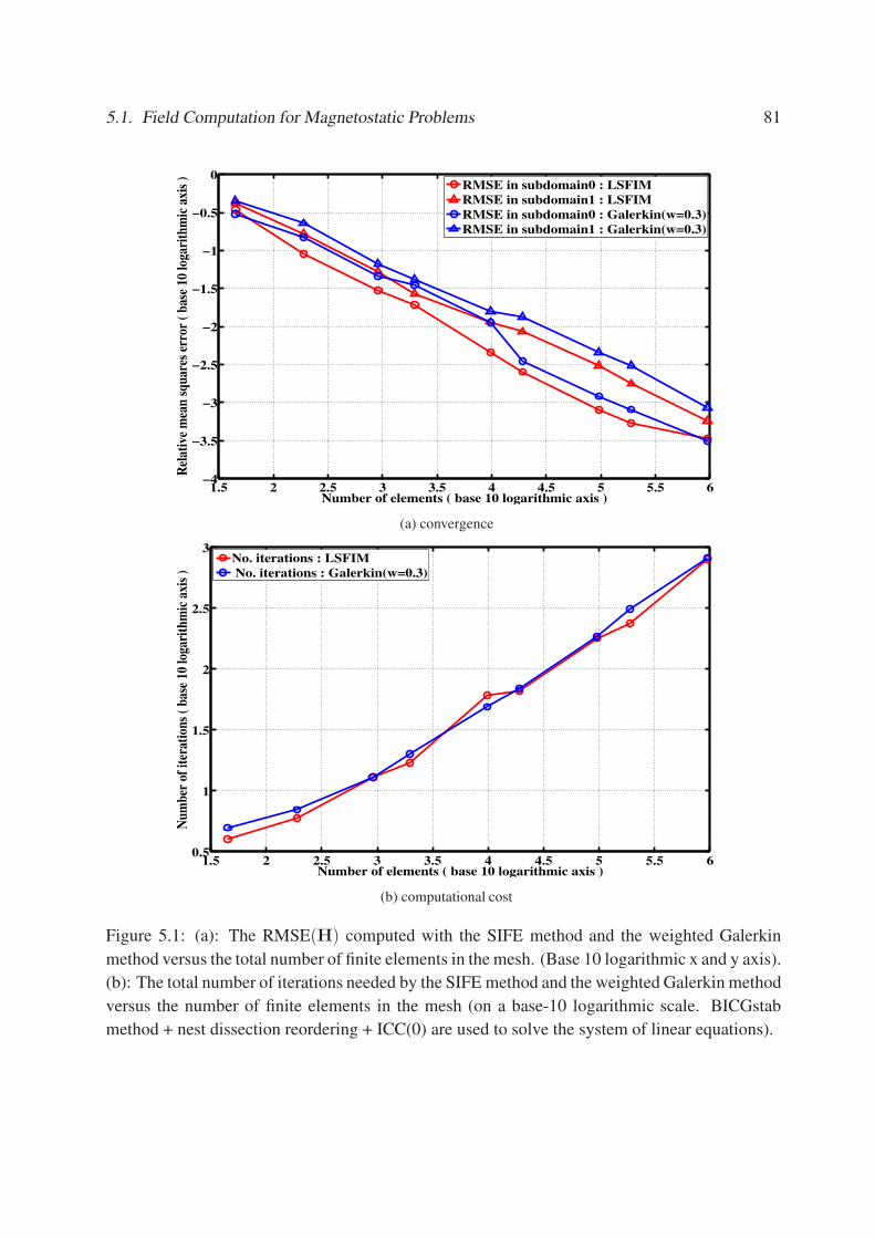
5.1. Field Computation for Magnetostatic Problems 81
1.5 2 2.5 3 3.5 4 4.5 5 5.5 6−4
−3.5
−3
−2.5
−2
−1.5
−1
−0.5
0
Number of elements ( base 10 logarithmic axis )
Rel
ativ
e m
ean
sq
uar
es e
rror
( b
ase
10 l
ogar
ith
mic
axi
s )
RMSE in subdomain0 : LSFIM
RMSE in subdomain1 : LSFIM
RMSE in subdomain0 : Galerkin(w=0.3)
RMSE in subdomain1 : Galerkin(w=0.3)
(a) convergence
1.5 2 2.5 3 3.5 4 4.5 5 5.5 60.5
1
1.5
2
2.5
3
Number of elements ( base 10 logarithmic axis )
Nu
mb
er o
f it
erat
ion
s (
bas
e 10
log
arit
hm
ic a
xis
)
No. iterations : LSFIM
No. iterations : Galerkin(w=0.3)
(b) computational cost
Figure 5.1: (a): The RMSE(H) computed with the SIFE method and the weighted Galerkin
method versus the total number of finite elements in the mesh. (Base 10 logarithmic x and y axis).
(b): The total number of iterations needed by the SIFE method and the weighted Galerkin method
versus the number of finite elements in the mesh (on a base-10 logarithmic scale. BICGstab
method + nest dissection reordering + ICC(0) are used to solve the system of linear equations).

82 Chapter 5. Electromagnetic Field Computations
Table 5.1: The two sub-domains and their relative permeability values
Di Definition of sub-domains µr
D0 0 ≤ x1 < 0.5 and 0 ≤ x2 < 0.5 and 0 ≤ x3 ≤ 0.5 1000
D1 0.5 < x1 ≤ 1 or 0.5 < x2 ≤ 1 and 0 ≤ x3 ≤ 0.5 1
To show the necessity of using hybrid finite elements, we compute the magnetic field strength in
this configuration with the SIFE method based on hybrid elements, the SIFE method based on
nodal elements and the weighted Galerkin method also based on nodal elements. In Fig. 5.2, we
show magnitude plots of the magnetic field strength computed by these methods. As shown in
Fig. 5.2(a), the analytic magnetic field strength suddenly reduces in the area with high perme-
ability. For the weighted Galerkin method, its solution is more or less correct in D1, but totally
wrong in D0. For the least-squares SIFE method based on nodal elements, the solution is not
correct in D1 and D0, but the magnitude of the solution does not differ too much from that of the
analytic solution. Only the magnetic field strength computed by the SIFE method based on hy-
brid elements agrees very well with the analytic solution. In Fig. 5.3(a), we show the RMSE and
it is clear that the solutions of the weighted Galerkin and the SIFE method both based on nodal
elements are not accurate at all. For the weighted Galerkin method, the solution in sub-domain1
converges very slowly while the solution in D0 makes no sense. For the SIFE method based on
nodal elements, the solution is equally bad in both sub-domains, but the magnitude of the com-
puted solution does not differ too much from the analytic one. It is also clear from Fig. 5.3(a) that
the SIFE method based on hybrid finite elements maintains the optimal convergence rate which is
of order O(h2) in both sub-domains. However, nothing comes for free. As shown in Fig. 5.3(b),
the BICGstab linear iterative solver for the SIFE method based on hybrid finite elements has to
use incomplete CC with fill level 2 to reach the same convergence level (10−12). Otherwise, it
is very difficult to find the solution. Fortunately, the order of the computational costs does not
change, it is still of order O(h−2).
5.1.3 Configuration with Extremely High Contrast
To test the limit of the SIFE method based on hybrid elements in handling extremely high con-
trast, we take the same configuration as in Section 5.1.2, except now the relative permeability in
homogeneous sub-domain 0 will range from 1 to 1 × 10¹¹ (as shown in Tab. 5.2). We conduct
a series of numeric experiments with the same interface conforming mesh as shown in Fig. 5.4.
We compare the SIFE method based on hybrid elements with the SIFE method and the weighted
(weighting factor 0.3) Galerkin method both based on nodal elements. Throughout these experi-
ments, the relative permeability in homogeneous subdomain D0 is increased from 1 to 1 × 10¹¹.
To draw a fair comparison, BICGstab linear iterative solver plus nested dissection reordering and
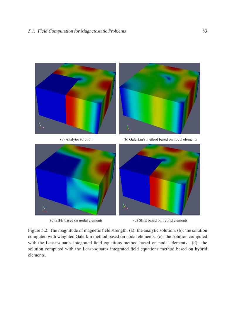
5.1. Field Computation for Magnetostatic Problems 83
(a) Analytic solution (b) Galerkin’s method based on nodal elements
(c) SIFE based on nodal elements (d) SIFE based on hybrid elements
Figure 5.2: The magnitude of magnetic field strength. (a): the analytic solution. (b): the solution
computed with weighted Galerkin method based on nodal elements. (c): the solution computed
with the Least-squares integrated field equations method based on nodal elements. (d): the
solution computed with the Least-squares integrated field equations method based on hybrid
elements.
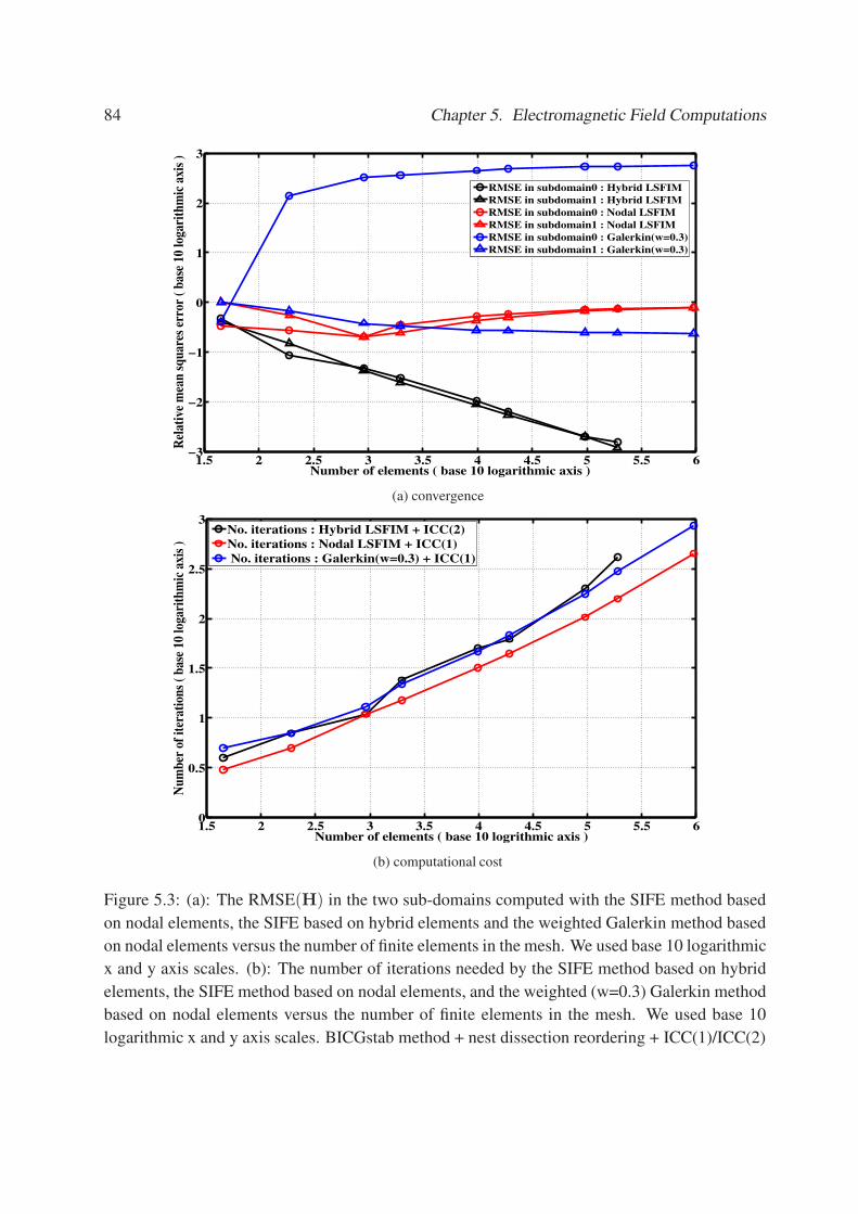
84 Chapter 5. Electromagnetic Field Computations
1.5 2 2.5 3 3.5 4 4.5 5 5.5 6−3
−2
−1
0
1
2
3
Number of elements ( base 10 logarithmic axis )
Rel
ativ
e m
ean
sq
uar
es e
rror
( b
ase
10 l
ogar
ith
mic
axi
s )
RMSE in subdomain0 : Hybrid LSFIM
RMSE in subdomain1 : Hybrid LSFIM
RMSE in subdomain0 : Nodal LSFIM
RMSE in subdomain1 : Nodal LSFIM
RMSE in subdomain0 : Galerkin(w=0.3)
RMSE in subdomain1 : Galerkin(w=0.3)
(a) convergence
1.5 2 2.5 3 3.5 4 4.5 5 5.5 60
0.5
1
1.5
2
2.5
3
Number of elements ( base 10 logrithmic axis )
Nu
mb
er o
f it
erat
ion
s (
bas
e 10
log
arit
hm
ic a
xis
)
No. iterations : Hybrid LSFIM + ICC(2)
No. iterations : Nodal LSFIM + ICC(1)
No. iterations : Galerkin(w=0.3) + ICC(1)
(b) computational cost
Figure 5.3: (a): The RMSE(H) in the two sub-domains computed with the SIFE method based
on nodal elements, the SIFE based on hybrid elements and the weighted Galerkin method based
on nodal elements versus the number of finite elements in the mesh. We used base 10 logarithmic
x and y axis scales. (b): The number of iterations needed by the SIFE method based on hybrid
elements, the SIFE method based on nodal elements, and the weighted (w=0.3) Galerkin method
based on nodal elements versus the number of finite elements in the mesh. We used base 10
logarithmic x and y axis scales. BICGstab method + nest dissection reordering + ICC(1)/ICC(2)

5.1. Field Computation for Magnetostatic Problems 85
Table 5.2: Configuration of the two sub-domains with extreme contrast
Di Definition of sub-domains µr
D0 0 ≤ x1 < 0.5 and 0 ≤ x2 < 0.5 and 0 ≤ x3 ≤ 1 1 ∼ 1 × 10¹¹
D1 0.5 < x1 ≤ 1 or 0.5 < x2 ≤ 1 and 0 ≤ x3 ≤ 1 1
Figure 5.4: The tetrahedron mesh. The mesh is interface conforming and contains 1973 nodes
and 9773 tetrahedrons. The gray area is sub-domain0. The green area is sub-domain1.
ICC(2) are used for all these methods.
As shown in Figure 5.5(a), the relative root mean square error in sub-domain0 computed
with the weighted Galerkin method based on nodal elements increases with the contrast ratio,
while the relative root mean square error in sub-domain1 stays stable, however incorrect. For the
SIFE method based on nodal elements, the relative root mean square errors in both sub-domains
stay stable and are not correct. For the SIFE method based on hybrid elements, the solution in
sub-domain0 and sub-domain1 stays stable and accurate, RMSE(H, 0) ≈ 10−2,RMSE(H, 1) ≈10−2. Its solution becomes inaccurate in the case of extremely high contrast 1012 because we im-
plement the boundary condition as additional equations of constraints as shown in Section 4.1.4.
With the presence of extremely high relative permeability, some off-diagonal entries of the sys-
tem matrix obtained by the SIFE method based on hybrid elements are comparable with the
weighting factor for the boundary conditions, which is approximately 1020. In these extreme
cases, the boundary conditions as additional equations will fail and the system matrix is close to
singular. The same phenomena can be observed in Fig. 5.5(b). Note that the total number of iter-
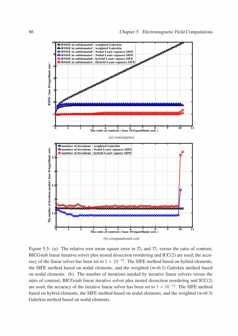
86 Chapter 5. Electromagnetic Field Computations
0 1 2 3 4 5 6 7 8 9 10 11−4
−2
0
2
4
6
8
10
The ratio of contrast ( base 10 logarithmic axis )
RM
SE
( b
ase
10 l
ogar
ith
mic
axi
s )
RMSE in subdomain0 : weighted Galerkin
RMSE in subdomain1 : weighted Galerkin
RMSE in subdomain0 : Nodal Least−squares SIFE
RMSE in subdomain1 : Nodal Least−squares SIFE
RMSE in subdomain0 : hybrid Least−square SIFE
RMSE in subdomain1 : Hybrid Least−squares SIFE
(a) convergence
0 1 2 3 4 5 6 7 8 9 10 111
1.5
2
2.5
3
3.5
4
The ratio of contrast ( base 10 logarithmic axis )
Th
e n
um
ber
of
iter
atio
ns
nee
ded
( b
ase
10 l
ogar
ith
mic
axi
s)
number of iterations : weighted Galerkin
number of iterations : Nodal Least−squares SIFE
number of iterations : hybrid Least−square SIFE
(b) computational cost
Figure 5.5: (a): The relative root mean square error in D0 and D1 versus the ratio of contrast.
BICGstab linear iterative solver plus nested dissection reordering and ICC(2) are used; the accu-
racy of the linear solver has been set to 1 × 10⁻¹². The SIFE method based on hybrid elements,
the SIFE method based on nodal elements, and the weighted (w=0.3) Galerkin method based
on nodal elements. (b): The number of iterations needed by iterative linear solvers versus the
ratio of contrast; BICGstab linear iterative solver plus nested dissection reordering and ICC(2)
are used; the accuracy of the iterative linear solver has been set to 1 × 10⁻¹². The SIFE method
based on hybrid elements, the SIFE method based on nodal elements, and the weighted (w=0.3)
Galerkin method based on nodal elements.

5.2. Field Computation in the Frequency Domain 87
Table 5.3: Configuration of the four sub-domains
Di Definition of subdomains εr σ µr
D1 0 ≤ x1 < 0.5, 0 ≤ x2 < 0.5, 0 ≤ x3 ≤ 1 1 0 1000
D2 0.5 ≤ x1 < 1, 0 ≤ x2 < 0.5, 0 ≤ x3 ≤ 1 1 0 1
D3 0 ≤ x1 < 0.5, 0.5 ≤ x2 < 1, 0 ≤ x3 ≤ 1 1 0 1
D4 0.5 ≤ x1 < 1, 0.5 ≤ x2 < 1, 0 ≤ x3 ≤ 1 1 0 10
ations needed shoots up when the ratio contrast is close to 1011, in which case some off-diagonal
entries of the system matrix are comparable with the weighting factor (1020) for the boundary
conditions as addition equations. Also note that the computational cost for the SIFE method
based on hybrid elements is higher than the other two methods. However, the computational cost
of the SIFE method based on hybrid elements does not increase with the contrast ratio.
5.2 Field Computation in the Frequency Domain
In this section, we apply the SIFE method to three-dimensional electromagnetic test configura-
tions in the frequency domain. We compare the SIFE method based on hybrid elements presented
in Section 4.2 with the SIFE method and the weighted Galerkin method both based on nodal el-
ements. Then we study the accuracy and efficiency of the SIFE method applied in the frequency
domain.
5.2.1 Configuration with High Contrast
In this experiment we verify the accuracy and convergence of the spatial discretization scheme
with a simple test case involving high contrasts. In the articles by Mur [22, 25] and the thesis
by Jorna [26], this test configuration has been used to examine the capabilities of the various
numerical methods developed to calculate the electromagnetic field in inhomogeneous media.
The theoretical solution is a harmonic solution at a single frequency. The domain of interest
is D = 0 ≤ x1 ≤ 1, 0 ≤ x2 ≤ 1, 0 ≤ x3 ≤ 1 and we use perfect electrically conducting
material boundary conditions at ∂D. Let the source density distributions be given by:
Jimp(x, ω) = −[σ(x) + jωε(x) +
2π2
jωµ(x)
]sin(πx1) sin(πx2)i3,
where ω = 2πf is the angular frequency and f = 1GHz. For such a source, the exact field
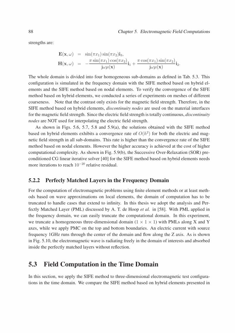
88 Chapter 5. Electromagnetic Field Computations
strengths are:
E(x, ω) = sin(πx1) sin(πx2)i3,
H(x, ω) = −π sin(πx1) cos(πx2)
jωµ(x)i1 +
π cos(πx1) sin(πx2)
jωµ(x)i2.
The whole domain is divided into four homogeneous sub-domains as defined in Tab. 5.3. This
configuration is simulated in the frequency domain with the SIFE method based on hybrid el-
ements and the SIFE method based on nodal elements. To verify the convergence of the SIFE
method based on hybrid elements, we conducted a series of experiments on meshes of different
coarseness. Note that the contrast only exists for the magnetic field strength. Therefore, in the
SIFE method based on hybrid elements, discontinuity nodes are used on the material interfaces
for the magnetic field strength. Since the electric field strength is totally continuous, discontinuity
nodes are NOT used for interpolating the electric field strength.
As shown in Figs. 5.6, 5.7, 5.8 and 5.9(a), the solutions obtained with the SIFE method
based on hybrid elements exhibits a convergence rate of O(h2) for both the electric and mag-
netic field strength in all sub-domains. This rate is higher than the convergence rate of the SIFE
method based on nodal elements. However the higher accuracy is achieved at the cost of higher
computational complexity. As shown in Fig. 5.9(b), the Successive Over-Relaxation (SOR) pre-
conditioned CG linear iterative solver [40] for the SIFE method based on hybrid elements needs
more iterations to reach 10−20 relative residual.
5.2.2 Perfecly Matched Layers in the Frequency Domain
For the computation of electromagnetic problems using finite element methods or at least meth-
ods based on wave approximations on local elements, the domain of computation has to be
truncated to handle cases that extend to infinity. In this thesis we adopt the analysis and Per-
fectly Matched Layer (PML) discussed by A. T. de Hoop et al. in [58]. With PML applied in
the frequency domain, we can easily truncate the computational domain. In this experiment,
we truncate a homogeneous three-dimensional domain (1 × 1 × 1) with PMLs along X and Y
axes, while we apply PMC on the top and bottom boundaries. An electric current with source
frequency 1GHz runs through the center of the domain and flow along the Z axis. As is shown
in Fig. 5.10, the electromagnetic wave is radiating freely in the domain of interests and absorbed
inside the perfectly matched layers without reflection.
5.3 Field Computation in the Time Domain
In this section, we apply the SIFE method to three-dimensional electromagnetic test configura-
tions in the time domain. We compare the SIFE method based on hybrid elements presented in

5.3. Field Computation in the Time Domain 89
E(real) E(imaginary)
H(real) H(imaginary)
Figure 5.6: The snapshots of the magnitude of the electric field strength and magnetic field
strength computed with the SIFE method based on hybrid elements.

90 Chapter 5. Electromagnetic Field Computations
2.5 3 3.5 4 4.5 5 5.5−3
−2.5
−2
−1.5
−1
−0.5
0
Total number of elements (base 10 logarithmic axis)
Rel
ativ
e m
ean
sq
uar
e er
ror
(bas
e 1
0 l
og
arit
hm
ic a
xis
)
Total RMSE(H) − Hybrid SIFE
Total RMSE(H) − Nodal SIFE
Total RMSE(E) − Hybrid SIFE
Total RMSE(E) − Nodal SIFE
(a)Relative mean square error in the whole domain of computation
2.5 3 3.5 4 4.5 5 5.5−3
−2.5
−2
−1.5
−1
−0.5
0
0.5
Total number of elements (base 10 logarithmic axis)
Rel
ativ
e m
ean
sq
uar
e er
ror
(bas
e 1
0 l
og
arit
hm
ic a
xis
)
RMSE(H) in D1 − Hybrid SIFE
RMSE(H) in D1 − Nodal SIFE
RMSE(E) in D1 − Hybrid SIFE
RMSE(E) in D1 − Nodal SIFE
(b)Relative mean square error in D1
Figure 5.7: Relative mean square error plots for the whole domain of computation and Sub-
domain 1.

5.3. Field Computation in the Time Domain 91
2.5 3 3.5 4 4.5 5 5.5−3
−2.5
−2
−1.5
−1
−0.5
0
Total number of elements (base 10 logarithmic axis)
Rel
ativ
e m
ean
sq
uar
e er
ror
(bas
e 1
0 l
og
arit
hm
ic a
xis
)
RMSE(H) in D
2 − Hybrid SIFE
RMSE(H) in D2 − Nodal SIFE
RMSE(E) in D2 − Hybrid SIFE
RMSE(E) in D2 − Nodal SIFE
(a)Relative mean square error in D2
2.5 3 3.5 4 4.5 5 5.5−3
−2.5
−2
−1.5
−1
−0.5
0
Total number of elements (base 10 logarithmic axis)
Rel
ativ
e m
ean
sq
uar
e er
ror
(bas
e 1
0 l
og
arit
hm
ic a
xis
)
RMSE(H) in D
3 − Hybrid SIFE
RMSE(H) in D3 − Nodal SIFE
RMSE(E) in D3 − Hybrid SIFE
RMSE(E) in D3 − Nodal SIFE
(b)Relative mean square error in D3
Figure 5.8: Relative mean square error plots for Sub-domain 2 and Sub-domain 3.

92 Chapter 5. Electromagnetic Field Computations
2.5 3 3.5 4 4.5 5 5.5−3
−2.5
−2
−1.5
−1
−0.5
0
Total number of elements (base 10 logarithmic axis)
Rel
ativ
e m
ean
sq
uar
e er
ror
(bas
e 1
0 l
og
arit
hm
ic a
xis
)
RMSE(H) in D
4 − Hybrid SIFE
RMSE(H) in D4 − Nodal SIFE
RMSE(E) in D4 − Hybrid SIFE
RMSE(E) in D4 − Nodal SIFE
(a)Relative mean square error in D4
2.5 3 3.5 4 4.5 5 5.51.8
2
2.2
2.4
2.6
2.8
3
3.2
Total number of elements (base 10 logarithmic axis)
To
tal
nu
mb
er o
f it
erat
ion
s (b
ase
10
lo
gar
ith
mic
ax
is)
Iterations needed for Hybrid SIFE+CG+SOR
Iterations needed for Nodal SIFE+CG+SOR
(b)Total number of iterations needed
Figure 5.9: Relative mean square error plot for Sub-domain 4 and the total number of iterations
needed when solving the systems with the CG+SOR method.

5.3. Field Computation in the Time Domain 93
Figure 5.10: Plots of the electric and magnetic field strengths in the existence of perfectly
matched layers.
Section 4.3 with the SIFE method based on nodal elements and the weighted Galerkin method
also based on nodal elements. Then we study the stability, accuracy and efficiency of the SIFE
method applied in the time domain.
5.3.1 Homogeneous Configuration
First, we consider a homogeneous configuration as a reference for further numeric experiments.
We test our method on (very rare) examples of a situation with analytic solutions, in order to
gauge the time domain stability and convergence of the SIFE method.
Steady State Configuration
The theoretical solution is a ‘steady state’ solution at a single frequency, containing a source term
that continuously injects current. Since we look for a time-domain solution, we use the steady
solution at t = 0 as initial state, and then start integrating from there in the time domain. The
configuration is a domain D = 0 ≤ x1 ≤ 1, 0 ≤ x2 ≤ 1, 0 ≤ x3 ≤ 0.5 bounded by PEC
material boundary conditions and consisting of vacuum. Let
h(x, t) =1
µ(x)ωsin(ωt),
g(x, t) = σ(x) cos(ωt) − ε(x)ω sin(ωt),
and let the external electric current density be given by:
Jimp(x, t) = [−2π2h(x, t) − g(x, t)] sin(πx1) sin(πx2)i3. (5.5)
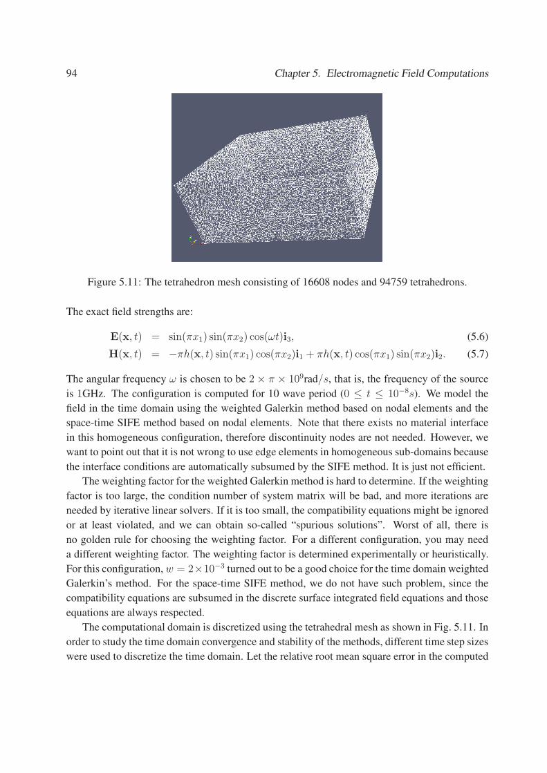
94 Chapter 5. Electromagnetic Field Computations
Figure 5.11: The tetrahedron mesh consisting of 16608 nodes and 94759 tetrahedrons.
The exact field strengths are:
E(x, t) = sin(πx1) sin(πx2) cos(ωt)i3, (5.6)
H(x, t) = −πh(x, t) sin(πx1) cos(πx2)i1 + πh(x, t) cos(πx1) sin(πx2)i2. (5.7)
The angular frequency ω is chosen to be 2 × π × 109rad/s, that is, the frequency of the source
is 1GHz. The configuration is computed for 10 wave period (0 ≤ t ≤ 10−8s). We model the
field in the time domain using the weighted Galerkin method based on nodal elements and the
space-time SIFE method based on nodal elements. Note that there exists no material interface
in this homogeneous configuration, therefore discontinuity nodes are not needed. However, we
want to point out that it is not wrong to use edge elements in homogeneous sub-domains because
the interface conditions are automatically subsumed by the SIFE method. It is just not efficient.
The weighting factor for the weighted Galerkin method is hard to determine. If the weighting
factor is too large, the condition number of system matrix will be bad, and more iterations are
needed by iterative linear solvers. If it is too small, the compatibility equations might be ignored
or at least violated, and we can obtain so-called “spurious solutions”. Worst of all, there is
no golden rule for choosing the weighting factor. For a different configuration, you may need
a different weighting factor. The weighting factor is determined experimentally or heuristically.
For this configuration, w = 2×10⁻³ turned out to be a good choice for the time domain weighted
Galerkin’s method. For the space-time SIFE method, we do not have such problem, since the
compatibility equations are subsumed in the discrete surface integrated field equations and those
equations are always respected.
The computational domain is discretized using the tetrahedral mesh as shown in Fig. 5.11. In
order to study the time domain convergence and stability of the methods, different time step sizes
were used to discretize the time domain. Let the relative root mean square error in the computed

5.3. Field Computation in the Time Domain 95
field strengths E,H in the whole space-time domain be:
RMSE(E) =
(∫t∫D|E(x, t) −Eexact(x, t)|2dVdt∫t∫D |Eexact(x, t)|2dVdt
) 1
2
,
RMSE(H) =
(∫t∫D |H(x, t) −Hexact(x, t)|2dVdt∫
t∫D |Hexact(x, t)|2dVdt
) 1
2
.
As shown in Fig. 5.12(a), the SIFE method converges very nicely as the time step size decreases,
and the RMSE in E and H are of order O(∆t2), which is the best one can get in case of linear
approximation. The convergence plot of the weighted Galerkin’s method is quite different. The
RMSE decreases with the time step size to a minimum and then increases. For the RMSE in E,
the accuracy might even be better than the SIFE method, because in this configuration, the elec-
tric field strength is always divergence free. However the divergence of magnetic flux might not
be zero if the compatibility relations are not respected in the computation. Therefore, the accu-
racy of H computed with Galerkin’s method is not as good due to the violation of compatibility
relations.
For the computational cost, as shown in Fig. 5.12(b), surprising enough, a smaller time step
size for the SIFE method does not necessarily increase the computational cost. The reason is that
as the time step size decreases, the solution at the current instance does not differ much from the
solution of the last instance and therefore less iterations are needed to get an acceptable solution.
Moreover, the computed field strengths are also more accurate. In addition to this, a smaller time
step allows us to use a coarser preconditioner. As a consequence, the total number of iterations
needed by Galerkin’s method is much more than that needed by the SIFE method. Considering
the fact that the SIFE method produces symmetric positive definite matrix and ICC factorization
can be used as preconditioner, the computational costs for the SIFE method are much less than
the costs for the weighted Galerkin’s method.
5.3.2 Configuration with High Contrast
In this experiment we verify the accuracy and convergence of the temporal discretization scheme
with the “steady-state” solution presented in Section 5.2.1. To achieve this we compute the steady
state solution in the time domain. We use the steady solution at t = 0 as initial state, and then
use the trapezoidal time-stepping scheme. DomainD is discretized with an interface conforming
tetrahedron mesh (5853 nodes and 30208 tetrahedrons). Once again, in the SIFE method based
on hybrid elements, discontinuity nodes are used only when interpolating the magnetic field
strength on the interfaces of discontinuity, and only continuity nodes are used for interpolating
the electric field strength as it is always continuous. The electromagnetic field quantities are
computed on a time interval consisting of 10 wave periods using different sizes for the time step.
As shown in Fig. 5.13(a), the SIFE method based on hybrid elements has second order accu-
racy in time even in the presence of high contrast. Note that at the right end of Fig. 5.13(b), the

96 Chapter 5. Electromagnetic Field Computations
−10.6−10.5−10.4−10.3−10.2−10.1−10−9.9−9.8−9.7−9.6−2.5
−2
−1.5
−1
−0.5
0
time step size ( base 10 logarithmic axis )
Sp
ace−
tim
e R
MS
E (
bas
e 10
log
arit
hm
ic a
xis
)
RMSE in E : computed with Galerkin
RMSE in H : computed with Galerkin
RMSE in E : computed with LSFIM
RMSE in H : computed with LSFIM
(a) convergence
0.20.40.60.811.21.41.61.82
x 10−10
0
1000
2000
3000
4000
5000
6000
7000
Time step size (s)
tota
l n
um
ber
of
Iter
atio
ns
nee
ded
Total number of iterations needed by Galerkin
Total number of iterations needed by LSFIM
(b) computational cost
Figure 5.12: RMSE versus time step size; Base 10 logarithmic x and y axis (a). The total
number of iterations needed versus time step size; BICGstab iterative solver and ICC(0) is used
for the least-squares SIFE method, BICGstab iterative solver and ILU(0) is used for the weighted
Galerkin’s method. The accuracy of these iterative solvers is set to be 10−12 (b).
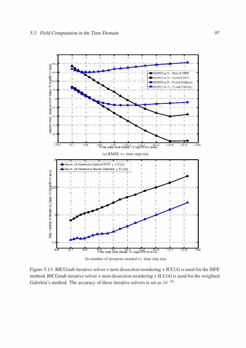
5.3. Field Computation in the Time Domain 97
(a) RMSE vs. time step size
(b) number of iterations needed vs. time step size
Figure 5.13: BICGstab iterative solver + nest-dissection reordering + ICC(4) is used for the SIFE
method, BICGstab iterative solver + nest-dissection reordering + ILU(4) is used for the weighted
Galerkin’s method. The accuracy of these iterative solvers is set as 10−20.

98 Chapter 5. Electromagnetic Field Computations
(a) Electric field strength (b) Magnetic field strength
Figure 5.14: Snapshot of the electric field strength and magnetic field strength computed with
the SIFE method at t = 8.25 × 10⁻⁹s (magnitude plots).
low-pass filter layout a coarse mesh
Figure 5.15: Details of the low-pass filter and the coarse mesh that is used. This filter is taken
from [1].
convergence curve is essentially flat. At this point the time discretization error is smaller than
the spatial discretization error and the latter error dominates. Finally, as shown in Fig. 5.13, the
computational cost of the SIFE method is comparable with the weighted Galerkin method, due
to the fact that symmetric preconditioners and CG method can be used for the SIFE method. A
snapshot of the magnitude of the electric and magnetic field strengths computed with the SIFE
method is shown in Fig. 5.14.
5.3.3 Microstrip Low-Pass Filter Simulated in the Time Domain
In this section we simulate the response of the low-pass filter shown in Fig. 5.15. This filter is

5.3. Field Computation in the Time Domain 99
t = 75ps t = 125ps
t = 175ps t = 225ps
Figure 5.16: The distribustion of Ez(x, t) just underneath the dielectric interface. Red color
indicates positive values and blue color indicates negative values.
fed by an electric field strength given by:
E(x, t) = A
√e
2θ
d
dtexp [−θ(t − t0)
2]iz, ∀x ∈ source plane,
where A is the amplitude, θ = 2π2f 2peak
, fpeak = 10 GHz, t0 = 0.1ns, and the low-pass filter
is truncated with a short circuit to the ground plane. The remaining boundary conditions are set
up according to the Electromagnetic Circuit Element concept (for details, we refer the reader to
[61]). The conductor is modeled as a perfect conductor and discontinuity nodes are used for inter-
polating electric field strengths on the interface of the substrate and the interface of the conductor.
The whole domain is discretized into 259568 tetrahedrons, the time step size used is 2.5ps, and
the configuration is simulated in the time domain for 5ns (2000 time steps). Fig. 5.16 shows the
distribution of Ez(x, t) just underneath the dielectric interface at t = 75ps, 125ps, 175ps, 225ps.
5.3.4 Perfecly Matched Layers in the Time Domain
With the leap-frog scheme for discretizing the time axis, we implemented the perfectly matched
layers for the 2D SIFE method in the time domain. To test the effectiveness of the perfectly

100 Chapter 5. Electromagnetic Field Computations
Figure 5.17: The loss profile of the two-dimensional Perfectly Matched Layers.
matched layers, we consider a configuration consisting of a square domain Ω = 0.1 ≤ x ≤0.9, 0.1 ≤ y ≤ 0.9 consisting of vaccum. The computational domain is surrounded by PMLs
DPML = 0 ≤ x ≤ 0.1 ∪ 0.9 ≤ x ≤ 1, 0 ≤ y ≤ 0.1 ∪ 0.9 ≤ y ≤ 1. The PML loss profile
is graded smoothly from 0 to σmax = 0.4257 by third order polynomials as shown in Fig. 5.17.
The external electric current density is given by
Jimpz = −χ(t)
√2θe(t − t0) exp[−θ(t − t0)
2]δ(x − 0.5)δ(y − 0.5),
where χ(t) is the Heaviside step function, the peak frequency fpeak is 1GHz, t0 = 2ns, θ =
2π2f 2peak
. We pick the observation points (0.6, 0.5) and (0.8, 0.5) and choose the observation
time interval long enough such that reflection (if any) can be well observed. The solutions com-
puted with and without PMLs are plotted in Fig.5.18.
5.4 Discussion
In this chapter, we presented a number of numeric experiments that demonstrate the accuracy,
efficiency and stability of the SIFE method in solving static and stationary EM problems, and EM
problems in both the time domain and frequency domain. Most of these experiments are based
on simple configurations for which analytic solutions are known. However, the existence of high
contrast interfaces makes these experiments difficult to handle with conventional computational
methods. With comparison to the analytic solutions, we measure the convergence of the SIFE
method exactly. Other than these, we conducted many other experiments with the simulation
package, however, the geometry we could simulate is limited by our simple layout-editorial
front-end.
In all the cases we computed, the SIFE method based on hybrid elements is superior to the
other alternative methods. Its computational complexity is comparable with the conventional

5.4. Discussion 101
0 1 2 3 4 5
x 10−9
−600
−400
−200
0
200
400
600
800
Time (S)
Ele
ctr
ic F
ield
Str
en
gth
(V
/m)
Electric field strength on point (0.6,0.5)
point(0.6,0.5) without PMLpoint(0.6,0,5) with PML
0 1 2 3 4 5
x 10−9
−300
−200
−100
0
100
200
300
400
500
Time (S)
Ele
ctr
ic F
ield
Str
en
gth
(V
/m)
Electric field strength on point (0.8,0.5)
point(0.8,0.5) without PMLpoint(0.8,0,5) with PML
Figure 5.18: The electric field strength at the observation points (0.6, 0.5) and (0.8, 0.5). The
Perfectly Matched Layers inDPML = 0 ≤ x ≤ 0.1∪0.9 ≤ x ≤ 1, 0 ≤ y ≤ 0.1∪0.9 ≤ y ≤ 1are of three elements thick. The maximum loss value within the PML is 0.4257.

102 Chapter 5. Electromagnetic Field Computations
Galerkin method, and it always converges to the analytical solution with the convergence rate of
order O(h2). Thus, we demonstrated with numeric experiments that this method indeed achieves
accurate field computations in cases with high contrast. Furthermore, this method is applicable
to practical situations.

Chapter 6
The Implementation of the Software Package
Many people tend to look at programming styles and
languages like religions: if you belong to one, you cannot
belong to others. But this analogy is another fallacy.
Niklaus Wirth
Up to this chapter, this thesis has been about algorithms and methods. For apparent reasons,
there is a strong interaction between the method and the implementation. A good algorithm
can easily be ruined by an inefficient implementation. Hence we feel a need to present our
implementation scheme as well as our implementation method, but we would like to point out
that our implementation scheme is neither the only nor the best for the SIFE method, but it
provides hopefully a better starting point for readers who do not want to learn how to do it in the
hard way as we did.
In the early stages of our research, we started with implementing a two dimensional EM
simulation package based on the SIFE method and hybrid elements using Matlab. It was a fast
prototype and positive results were obtained with the Matlab code. However, as we attempted
to move from 2D to 3D, the procedural programming method of Matlab became very difficult
to develop with and to maintain. The Matlab code appeared to be very slow and inefficient.
Later we understood that it was the dynamic memory allocation for the system matrices that
took the majority of the computational time. It is true that one can program efficient Matlab
code if one tries hard enough, but eventually we decided to move on to implement the three
dimensional electromagnetic simulation software package EMsolve3D in Object-Oriented C++,
because firstly the SIFE method consists of parts which can obviously be treated as objects,
e.g. domains, elements, analysis and secondly, we are more familiar with C++ for which some
excellent open source software packages such as Qt,OpenGL, and Petsc can be used.
In this chapter, we shall present our implementation scheme. However, we shall not focus on
the details of the implementation because the coding takes some ten thousand lines of C++ code.
Instead, we shall focus on the Object-Oriented design of the software package, inheritance of
the classes, collaboration between the classes and other abstract matters. Those are the common
features of Object-Oriented programming, and one can take exactly the same Object-Oriented
scheme and implement it with other OO programming languages, e.g. Java, but one might find
the memory management scheme in Java (i.e. dynamic allocation and garbage collector) to be
inappropriate in this case, in which frequent and massive memory allocation and de-allocation
103

104 Chapter 6. The Implementation of the Software Package
are needed to make the best of the limited memory. We tried to come up with an efficient
Object-Oriented design in terms of computational efficiency, memory and code efficiency, i.e.
extensibility and re-usability.
6.1 Object-Oriented Design of the Main Classes
As we have shown in previous sections, electromagnetic simulation problems consist of objects
such as a mesh that geometrically discretizes the computational domain, a physical model that
discretizes the physical solution, some boundary conditions and source terms, some linear solvers
and preconditioners, and degrees of freedom which are used to represent the approximated field
and so on. In this section, we present the classes that represent these objects in the Unified
Modeling Language (UML). Most of the time, the meaning or the purpose of each member is
clear from its name. For more details, we invite the interested reader to consult our source code
(for access, please contact us at [email protected]) and the full documentation of the
source code generated with Doxygen [62].
6.1.1 Domain, Mesh
In a bottom-up fashion, we begin by presenting the design of the Domain class.
Mesh File in the Neutral Volume Mesh Format
With a layout description of the computation domain, three dimensional tetrahedron meshes are
generated with msh developed by K.J. van der Kolk [63] or netgen [64]. The mesh file takes the
following neutral volume mesh format, which contains the following sections:
1. nodes
After the number of nodes there follows a list of x, y, and z-coordinates of the mesh-nodes.
2. volume elements
After the number of volume elements there follows a list of tetrahedrons. Each element is
specified by the sub-domain number, and 4 node indexes. The node indexes start with 1.
3. surface elements
After the number of surface elements there follows a list of triangles. Each element is
specified by the boundary condition number, and 3 node indexes. The node indexes start
with 1.

6.1. Object-Oriented Design of the Main Classes 105
Geometric Elements
Apparently a Domain consists of Elements, Nodes, Edges, and Facets, which are all Geometric
Elements. All of these have many things in common, e.g. an index and a label. Furthermore, each
one of these Geometric Elements can be associated with some degrees of freedom. Therefore a
base classGeometric element can be constructed as shown in Fig. 6.1. Minimum set of functions
and members are not assumed. With this class at hand, we may derive the classes Facet, Element,
Node and Edge as shown in Fig. 6.1. Since we are working with a three dimensional tetrahedral
mesh in this thesis, Tetrahedron and Triangle face are constructed as shown in Fig. 6.1. One may
extend this library with other shapes of elements and facets, if needed.
The hybrid tetrahedron TetHybrid and hybrid nodeNodeHybrid are also constructed as shown
in Fig. 6.1. They have basically the same functions as the normal tetrahedron Tetrahedron and
node Node, except that they may store more information about their neighboring tetrahedrons
and nodes. These objects are only needed where discontinuity nodes are assigned. This design
should save some computer memory because in a complicated tetrahedron mesh the number of
nodes and tetrahedrons can be great.
Domain, Material
The Domain class collects all the information about the discretized domain of computation and
the mesh. It maintains a list of nodes (Node), a list of edges (Edge), a list of facets (Facet) and a
list of elements (Element). Also it keeps a record of the list of boundary indexes and sub-domains
for which constitutive parameters (Material) are defined. The Domain class has a number of
functions that help to construct the mesh, such as add nodes(), add edges(), add elements(), etc,
and to analyze the mesh such as num of nodes(), num of edges(), num of elements(), etc. A
Domain object is often initialized with a certain mesh file in the neutral volume mesh format.
The Material class and the Domain class are designed as shown in Fig. 6.2(a) and Fig. 6.2(b).
Note that a domainMutex is assigned for the Domain class for multi-threaded computations.
Variables and Degrees of Freedom
As the field quantities are discretized, unknown coefficients or degrees of freedom are needed to
represent them. Depending on different discretization schemes, these degrees of freedom can be
associated with nodes, edges, facets or elements. Therefore, the base class Variable, Constraints
andDOF should be designed as shown in Fig. 6.3. TheConstraint represents boundary condition
values, thus they are the variables of which the value has been fixed. Each Variable has a unique
integer index indicating its position in the solution vector.

106 Chapter 6. The Implementation of the Software Package
libmices::Geometric_element
+ index
+ Geometric_element()+ get_axis()+ get_index()+ get_vars()+ output()+ permute_nodes()+ push_vars()+ removeDOF()+ set_index()+ type()+ write()+ ~Geometric_element()- operator=()
libmices::Edge
+ nodes
+ attach_node()+ Edge()+ get_end()+ get_from()+ length()+ num_of_nodes()+ permute_nodes()+ ~Edge()
libmices::Element
+ infoBuffer+ infoSet+ nodes+ subdomain
+ attach_node()+ center()+ Element()+ Element()+ get_edge()+ get_face()+ get_node()+ get_subdomain()+ get_surface()+ locateFacet()+ locateNode()+ num_of_edges()+ num_of_facets()+ num_of_nodes()+ set_node()+ set_subdomain()+ type()+ volume()+ ~Element()
libmices::Facet
+ nodes+ on_boundary# inWhichElement
+ attach_node()+ center()+ clearInElements()+ Facet()+ get_node()+ get_on_boundary()+ getInElements()+ num_of_edges()+ num_of_nodes()+ permute_nodes()+ set_node()+ set_on_boundary()+ setInElement()+ surface()+ type()+ ~Facet()
libmices::Node
+ coord+ in_which_domain+ on_which_boundary+ vars
+ get_in_domain()+ get_on_boundary()+ get_vars()+ getNbNeigNodes()+ getNeigNode()+ isInDomain()+ Node()+ output()+ push_vars()+ removeDOF()+ set_coord()+ set_in_domain()+ set_on_boundary()+ setNeigNode()+ type()+ write()+ ~Node()
libmices::Tetrahedron
# _compVolume# _surfaceMap# _volume
+ get_edge()+ get_face()+ get_node()+ get_surface()+ getNeigTet()+ num_of_edges()+ num_of_facets()+ output()+ permute_nodes()+ setNeigTet()+ Tetrahedron()+ Tetrahedron()+ type()+ volume()+ write()+ ~Tetrahedron()
libmices::TetHybrid
+ neigTets
+ getNeigTet()+ getNormalTetrahedron()+ setNeigTet()+ TetHybrid()+ TetHybrid()+ type()+ ~TetHybrid()
libmices::Triangle_face
+ num_of_edges()+ permute_nodes()+ surface()+ Triangle_face()+ type()+ write()
libmices::NodeHybrid
+ inElements+ neigNodes- nbNeigNodes
+ getNbNeigNodes()+ getNeigNode()+ getNormalNode()+ NodeHybrid()+ NodeHybrid()+ setInElement()+ setNeigNode()+ type()+ ~NodeHybrid()
Figure 6.1: Members and member functions of Geometric element, Facet, Element, Node, Edge,
Tetrahedron, Triangle face, TetHybrid and NodeHybrid. Hollow arrows indicate the relation of
inheritance.

6.1. Object-Oriented Design of the Main Classes 107
libmices::MaterialConstantIsotropic
- _eCon- _eps- _mCon- _mu- material_name
+ classType()+ e_conductivity()+ e_conductivity()+ e_conductivity()+ getParameters()+ info()+ m_conductivity()+ m_conductivity()+ m_conductivity()+ MaterialConstantIsotropic()+ MaterialConstantIsotropic()+ permeability()+ permeability()+ permeability()+ permittivity()+ permittivity()+ permittivity()+ resetParameters()+ set_eCon()+ set_eps()+ set_mCon()+ set_mu()+ set_name()+ shortInfo()+ ~MaterialConstantIsotropic()
libmices::Material
+ material_id
+ dump_info()+ e_conductivity()+ e_conductivity()+ e_conductivity()+ getParameters()+ hasPanel()+ m_conductivity()+ m_conductivity()+ m_conductivity()+ Material()+ Material()+ permeability()+ permeability()+ permeability()+ permittivity()+ permittivity()+ permittivity()+ set_e_conductivity()+ set_id()+ set_m_conductivity()+ set_permeability()+ set_permittivity()
(a)Material
libmices::Domain
+ boundaries+ domain_name+ edges+ elements+ facets+ materialPtrMap+ nodes+ subdomains# _dimension# _edges# _faces# _hybrid_nodes# _hybrid_tets# _nodes# _tets# being_used_by# domainMutex# scale
+ classType()+ decrease_used_by()+ dim()+ Domain()+ dump_info()+ get_axis()+ get_edge()+ get_element()+ get_facet()+ get_material_in_subdomain()+ get_node()+ get_scale()+ getMaterial()+ getParameters()+ hasPanel()+ increase_used_by()+ info()+ lock()+ num_of_boundaries()+ num_of_edges()+ num_of_elements()+ num_of_faces()+ num_of_facets()+ num_of_materials()+ num_of_nodes()+ num_of_subdomains()+ permute_nodes_of_elements()+ print()+ removeDOF()+ resetParameters()+ set_dim()+ set_id()+ set_material_in_subdomain()+ set_scale()+ setWidgetItem()+ unlock()+ used_by()+ ~Domain()# add_edge()# add_element()# add_facet()# add_node()# axis_x()# axis_y()# axis_z()# construct_from_mices_mesh()# construct_from_neutral_mesh()# insert_boundary()# insert_subdomain()# updateFaceInElements()
(b)Domain
libmices::Analysis
+ BConditionMap+ domain+ iteration+ ksp_config+ outputs+ pc_config+ problem_description+ RMSE1+ RMSE2+ SourceMap# _output# ierr# reason# symmetric
+ addBC()+ addSource()+ Analysis()+ clear()+ dump_info()+ getBC()+ getOnInterface()+ getParameters()+ getSource()+ getSource()+ hasPanel()+ info()+ num_of_BCs()+ resetParameters()+ set_description()+ set_domain()+ set_output()+ setWidgetItem()+ shortInfo()+ toHybridDomain()+ ~Analysis()# applyBCs()# applyBCs()# check_err()# checkconvergence()# NJcurrent()# Nkappa()# NKcurrent()# Nmagnetic()# Nsigma()# set_symmetric()# solve_equation()
(c)Analysis
Figure 6.2: Members and member functions ofMaterial, Domain and Analysis.

108 Chapter 6. The Implementation of the Software Package
libmices::Variable
+ index
+ get_constraint_value()+ get_index()+ set_constraint_value()+ set_index()+ type()+ Variable()+ ~Variable()
libmices::Constraint
- _value
+ Constraint()+ Constraint()+ get_constraint_value()+ set_constraint_value()+ type()
libmices::DOF
+ DOF()+ type()
Figure 6.3: Members and member functions of Variable, Constraint and DOF.
libmices::Analysis
libmices::Electromagnetics
libmices::ElectromagneticsFreq
libmices::Electrostatic
libmices::Magnetostatic
libmices::Electromagnetics_leapfrog
libmices::Electromagnetics_trape
libmices::Electrostatic_galerkin
libmices::Electrostatic_LSFIM
libmices::Magnetostatic_galerkin
libmices::Magnetostatic_LSFIM
Figure 6.4: The (partial) inheritance diagram of the EM solvers
6.1.2 Analysis, Electromagnetic Solvers
After the domain of computation has been discretized, the numeric analysis can begin. All elec-
tromagnetic solvers have some members and member functions in common such as boundary
conditions, system solution, normalization of the field quantities, and so on. Therefore, the
base class Analysis, on which all electromagnetic solvers derive from, should be constructed
as shown in Fig. 6.2(c). Then a number of electromagnetic solvers which solve electrostatic
problems, magnetostatic problems, electromagnetic problems in the time domain, and electro-
magnetic problems in the frequency domain can be derived as shown in Fig. 6.4. For the time
domain electromagnetic field solver, the time axis can be discretized with the trapezoidal rule
or with the leapfrog scheme. We also implemented electromagnetic field solvers based on the
Galerkin method for comparison purposes.

6.1. Object-Oriented Design of the Main Classes 109
libmices::Initial_value
+ description+ subdomain
+ classType()+ getParameters()+ hasPanel()+ Initial_value()+ shortInfo()+ value()+ value()
libmices::Dynamic_four_domain_E_value
- eps- FREQ- mu- omega- sigma_e- sigma_m
+ classType()+ Dynamic_four_domain_E_value()+ getParameters()+ resetParameters()+ value()- g()- h()
libmices::Dynamic_four_domain_H_value
- eps- FREQ- mu- omega- sigma_e- sigma_m
+ classType()+ Dynamic_four_domain_H_value()+ getParameters()+ resetParameters()+ value()- g()- h()
Figure 6.5: Inheritance diagram for the initial field values.
6.1.3 Initial Field, Boundary Conditions and Source Terms
The initial field value conditions for time domain electromagnetic solvers are constructed as
shown in Fig. 6.5.
The boundary conditions are constructed as shown in Fig. 6.6. With these classes, one can
define boundary conditions on the tangential component, boundary conditions on the normal
component, or define an internal interface of discontinuity. Note that the EMinterface class
defines an interface of discontinuity, on which either electric field strength or magnetic field
strength will be interpolated with discontinuity nodes.
The source terms in the electromagnetic solvers are to be defined as shown in Fig. 6.7. It
provides functions to obtain the electric charge densities, electric volume densities and magnetic
current densities at any given space(-time) coordinate.
6.1.4 KSP Linear Solvers and Preconditioners
The configuration of the linear solvers is defined as shown in Fig. 6.8. The implementation of
this module is via the numeric computation C++ library Petsc. For the types of Krylov space
iterative linear solvers, you can choose among KSPCG, KSPCGS, KSPBICG, KSPBCG-Stable,
KSPGMRES, KSPLSQR and so on. The solution tolerance and maximum iterations can also be
set accordingly.
The configuration of the preconditioners is defined as shown in Fig. 6.8. One can choose
among incomplete LU, incomplete CC, JACOBI and SSOR. The system matrix can be reordered

110 Chapter 6. The Implementation of the Software Package
libmices::BC
+ _index+ _on+ id# DIAG
+ applyPBC()+ applyPBC()+ applyPBC()+ applyPBC()+ BC()+ classType()+ dump_info()+ get_index()+ getParameters()+ hasPanel()+ IsInterface()+ on()+ set_index()+ set_on()+ shortInfo()+ type()# allBC()
libmices::BC_PNF
# _value# _weight# b# b2# M# M2
+ applyPBC()+ applyPBC()+ BC_PNF()+ classType()+ get_weight()+ getParameters()+ resetParameters()+ set_value()+ set_weight()+ type()+ ~BC_PNF()# applyBConElementFacet()# applyBConElementFacet()
libmices::BC_PTF
# _Tfield# _weight# b# b2# M# M2# tol
+ applyPBC()+ applyPBC()+ BC_PTF()+ BC_PTF()+ classType()+ get_weight()+ getParameters()+ resetParameters()+ set_value()+ set_weight()+ type()+ ~BC_PTF()# applyBConElementFacet()# applyBConElementFacet()# getTfield()
libmices::EMinterface
- weighting
+ classType()+ EMinterface()+ get_weighting()+ getParameters()+ IsInterface()+ resetParameters()+ set_weighting()+ type()
libmices::PBC
# PBCtable
+ applyPBC()+ applyPBC()+ classType()+ getParameters()+ PBC()+ resetParameters()+ setPBC()+ type()
libmices::BC_PTF_Edge
+ BC_PTF_Edge()+ IsInterface()
libmices::BC_RickerWaveletPTF
# freq# t# t0
+ applyPBC()+ applyPBC()+ BC_RickerWaveletPTF()+ BC_RickerWaveletPTF()+ classType()+ set_freq()+ setT()+ type()# getTfield()
libmices::BC_SinPTF
# freq# t# t0# t1
+ applyPBC()+ applyPBC()+ BC_SinPTF()+ BC_SinPTF()+ classType()+ getParameters()+ resetParameters()+ set_freq()+ setT()+ type()# getTfield()
libmices::BC_RickerWaveletPTF_Edge
+ BC_RickerWaveletPTF_Edge()+ BC_RickerWaveletPTF_Edge()+ IsInterface()
libmices::BC_SinPTF_Edge
+ BC_SinPTF_Edge()+ BC_SinPTF_Edge()+ IsInterface()
libmices::SinPBC
- freq- t0- t1
+ applyPBC()+ applyPBC()+ classType()+ getParameters()+ resetParameters()+ set_freq()+ setT()+ SinPBC()+ type()
Figure 6.6: Inheritance diagram for the boundary conditions.

6.2. Design of the Graphic User Interface 111
libmices::Source
+ source_id
+ classType()+ dump_info()+ electric_charge_density()+ electric_charge_density()+ electric_current_density()+ electric_current_density()+ electric_current_density()+ electric_current_density()+ getParameters()+ hasPanel()+ Jdensity()+ Jdensity()+ Kdensity()+ Kdensity()+ magnetic_charge_density()+ magnetic_charge_density()+ magnetic_current_density()+ magnetic_current_density()+ magnetic_current_density()+ shortInfo()+ Source()+ Source()# allSource()
libmices::ChargedSphere
+ ChargedSphere()+ ChargedSphere()+ classType()+ electric_charge_density()+ electric_current_density()+ electric_current_density()
libmices::Dynamic_four_domain_source
- eps- FREQ- mu- omega- sigma_e- sigma_m
+ classType()+ Dynamic_four_domain_source()+ Dynamic_four_domain_source()+ electric_current_density()+ getParameters()+ Jdensity()+ Jdensity()+ Kdensity()+ Kdensity()+ magnetic_current_density()+ resetParameters()- g()- h()
libmices::LineSource
+ Jdensity()+ Kdensity()+ LineSource()
libmices::Static_four_domain_source
- _mu
+ classType()+ electric_charge_density()+ electric_current_density()+ electric_current_density()+ getParameters()+ resetParameters()+ set_contrast()+ Static_four_domain_source()+ Static_four_domain_source()
Figure 6.7: Inheritance diagram for the sources.
with nested-dissection, 1WD, QMD or RCM. Basically, every iterative solver, preconditioner
and matrix reordering scheme that have been implemented in Petsc can be used transparently in
EMsolve3D.
6.2 Design of the Graphic User Interface
We implemented the graphic user interface with the help of Qt and OpenGL. For ease of mainte-
nance and extensibility, we designed the GUI in an Object-Oriented pattern.
6.2.1 Generic Class
A basic Generic class is constructed and all the classes that can be configured with the graphic
user interface are derived from this class, as shown in Fig. 6.9. All classes that are derived from
the Generic class are able to add a widget item to the simulation pipeline of the EMsolverMain-
Window class or to the the MeshViewer class, which are the GUI classes to visualize, configure
and manage the domain configurations and the solvers configurations.

112 Chapter 6. The Implementation of the Software Package
libmices::KSPconfig
+ ksp_tolerrance+ ksp_type+ max_iter
+ classType()+ configKSP()+ getParameters()+ hasPanel()+ KSPconfig()+ resetParameters()+ shortInfo()- allKSPtype()
Iterative solvers
libmices::PCconfig
+ fill_in_level+ fill_level+ ordering_type+ pc_type- symmetric
+ classType()+ configPC()+ getParameters()+ hasPanel()+ PCconfig()+ resetParameters()+ set_symmetric()+ shortInfo()- allPCtype()- allReordering()
Preconditioners
Figure 6.8: Members and member functions of the iterative linear solvers and preconditioners.
libmices::Generic
libmices::Analysis
libmices::BC
libmices::EMmodel
libmices::Initial_value
libmices::KSPconfig
libmices::Material
libmices::OutputBucket
libmices::PCconfig
libmices::Source
libmices::Generic
+ classType()+ decrease_used_by()+ dump_info()+ getParameters()+ hasPanel()+ increase_used_by()+ info()+ resetParameters()+ setWidgetItem()+ setWidgetItem()+ shortInfo()+ simulate()+ solve()+ stop()+ used_by()+ ~Generic()- operator=()
Figure 6.9: Inheritance diagram and the UML model of the Generic class.

6.2. Design of the Graphic User Interface 113
libmices::EMmodel
+ EMsolver+ thread
+ classType()+ dump_info()+ EMmodel()+ getParameters()+ hasPanel()+ resetParameters()+ setWidgetItem()+ setWidgetItem()+ shortInfo()+ solve()+ stop()+ ~EMmodel()
EMmodel
libmices::ComputeThread
- solver
+ ComputeThread()+ set_solver()# exec()# run()
ComputeThread
libmices::EMmodellibmices::Generic libmices::Analysis
libmices::OutputBucket
libmices::KSPconfig
libmices::Domain
libmices::PCconfig
libmices::ComputeThread
solver
EMsolver
outputs
ksp_configdomain
pc_config thread
QThread
Collaboration diagram for EMmodel
Figure 6.10: UML of EMmodel class and ComputeThread class. Collaboration diagram for
EMmodel.
6.2.2 EMmodel and ComputeThread
In our design, one Domain object can be associated with many electromagnetic solvers. For
instance, one may want to solve an electromagnetic problem both in the time domain and in the
frequency domain.
In the graphic user interface, these electromagnetic solvers are handled via the EMmodel
class. Each of its instances runs upon an individual thread ComputeThread. This means that
configuration of the GUI is possible when one EMmodel object is simulating. Multiple simula-
tions can run at the same time, therefore they make full use of the multi-core CPUs.
6.2.3 EMsolverMainWindow and MeshViewer
The design of the graphic user interface is shown in Fig. 6.11. OpenGL and Qt are used to
implement this graphic user interface under Linux. MeshViewer is a light graphic user interface
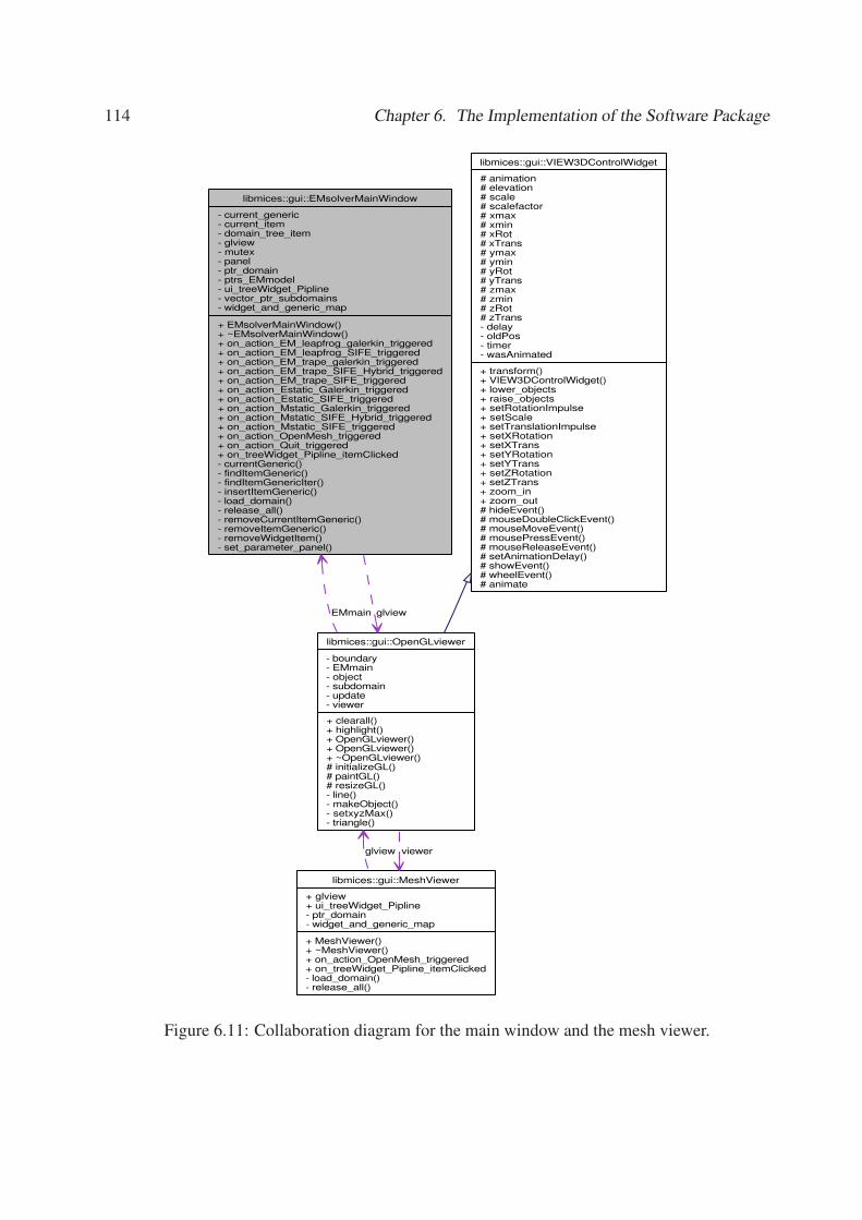
114 Chapter 6. The Implementation of the Software Package
libmices::gui::EMsolverMainWindow
- current_generic- current_item- domain_tree_item- glview- mutex- panel- ptr_domain- ptrs_EMmodel- ui_treeWidget_Pipline- vector_ptr_subdomains- widget_and_generic_map
+ EMsolverMainWindow()+ ~EMsolverMainWindow()+ on_action_EM_leapfrog_galerkin_triggered+ on_action_EM_leapfrog_SIFE_triggered+ on_action_EM_trape_galerkin_triggered+ on_action_EM_trape_SIFE_Hybrid_triggered+ on_action_EM_trape_SIFE_triggered+ on_action_Estatic_Galerkin_triggered+ on_action_Estatic_SIFE_triggered+ on_action_Mstatic_Galerkin_triggered+ on_action_Mstatic_SIFE_Hybrid_triggered+ on_action_Mstatic_SIFE_triggered+ on_action_OpenMesh_triggered+ on_action_Quit_triggered+ on_treeWidget_Pipline_itemClicked- currentGeneric()- findItemGeneric()- findItemGenericIter()- insertItemGeneric()- load_domain()- release_all()- removeCurrentItemGeneric()- removeItemGeneric()- removeWidgetItem()- set_parameter_panel()
libmices::gui::OpenGLviewer
- boundary- EMmain- object- subdomain- update- viewer
+ clearall()+ highlight()+ OpenGLviewer()+ OpenGLviewer()+ ~OpenGLviewer()# initializeGL()# paintGL()# resizeGL()- line()- makeObject()- setxyzMax()- triangle()
EMmain glview
libmices::gui::MeshViewer
+ glview+ ui_treeWidget_Pipline- ptr_domain- widget_and_generic_map
+ MeshViewer()+ ~MeshViewer()+ on_action_OpenMesh_triggered+ on_treeWidget_Pipline_itemClicked- load_domain()- release_all()
glview
libmices::gui::VIEW3DControlWidget
# animation# elevation# scale# scalefactor# xmax# xmin# xRot# xTrans# ymax# ymin# yRot# yTrans# zmax# zmin# zRot# zTrans- delay- oldPos- timer- wasAnimated
+ transform()+ VIEW3DControlWidget()+ lower_objects+ raise_objects+ setRotationImpulse+ setScale+ setTranslationImpulse+ setXRotation+ setXTrans+ setYRotation+ setYTrans+ setZRotation+ setZTrans+ zoom_in+ zoom_out# hideEvent()# mouseDoubleClickEvent()# mouseMoveEvent()# mousePressEvent()# mouseReleaseEvent()# setAnimationDelay()# showEvent()# wheelEvent()# animate
viewer
Figure 6.11: Collaboration diagram for the main window and the mesh viewer.

6.3. Programming Interface of EMsolve3D 115
Figure 6.12: The graphic user interface of EMsolve3D. At this moment, the software can be
used to solve magnetostatic, electrostatic, and electromagnetic time domain problems. All nec-
essary parameters can be configured with the parameter panel. Visualization of the mesh and the
simulation results is supported.
which only visualizes the three dimensional mesh. EMsolverMainWindow provides more panels
and functions to configure and manage computational domains and electromagnetic solvers.
6.2.4 Snapshot of the Graphic User Interface
At this moment, the software package EMsolve3D can be used to solve magnetostatic, electro-
static, and electromagnetic time domain problems. All necessary parameters can be configured
with the parameter panel. Visualization of the mesh is supported. Visualization of the computed
solution is supported via VTK and Paraview.
6.3 Programming Interface of EMsolve3D
With the EMsolve3D used as a simulation OO library, we can easily write C++ code that solves
the testing problems. The graphic user interface is still needed to visualize the mesh and identify
the indexes of boundaries and sub-domains. For a full account of the functions and classes, we
invite the interested reader to check the code documentation. Examples of using EMsolve3D
with function calls can be found in the source code. We also keep necessary interfaces open so
that the user can easily extend the library with his own classes.

116 Chapter 6. The Implementation of the Software Package
6.4 Discussion on the Implementation
Although the software package delivered some promising results, it is not really fine enough for
customers to use. Therefore, the entire C++ software package does not escape the fate of being
a prototype. A number of extensions and improvements can be applied. First, due to the fact
that we spent limited time on software testing, some bugs may still exist and a comprehensive
testing would be needed. Second, it would be very useful to extend the package with the ability
to work with hexahedral meshes or even meshes with mixed elements. Third, the functionality
of the graphic user interface should be enhanced. Fourth, a great addition to the package would
be an integrated layout editor and mesh generator. Fifth, to be able to handle more complicated
cases, the software package should be extended so as to work on parallel computers. For now,
we encourage the interested readers to obtain a copy of the software package, and we certainly
hope that this work can be carried on by successors.
Chapter 7
Algorithms to Solve Hierarchically Semi-separable
Systems
A mathematician is a device for turning coffee into theorems.
Paul Erdos
‘Hierarchical Semi Separable’ matrices (HSS matrices) form an important class of structured
matrices for which matrix transformation algorithms that are linear in the number of equations
(and a function of other structural parameters) can be given. In particular, a system of linear
equations Ax = b can be solved with linear complexity in the size of the matrix, the overall
complexity being linearly dependent on the defining data. Also, LU and ULV factorization
can be executed ‘efficiently’, meaning with a complexity linear in the size of the matrix. This
chapter gives a survey of the main results, including a proof for the formulas for LU-factorization
that were originally given in the thesis of Lyon [65], the derivation of an explicit algorithm
for ULV factorization and related Moore-Penrose inversion, a complexity analysis and a short
account of the connection between the HSS and the SSS (sequentially semi-separable) case. A
direct consequence of the computational theory is that from a mathematical point of view the
HSS structure is ‘closed’ for a number operations. The HSS complexity of a Moore-Penrose
inverse equals the HSS complexity of the original, for a sum and a product of operators the HSS
complexity is no more than the sum of the individual complexities1.
7.1 Introduction
The term ‘semi-separable systems’ originated in the work of Gohberg, Kailath and Koltracht [46]
where these authors remarked that if an integral kernel is approximated by an outer sum, then the
system could be solved with a number of operations essentially determined by the order of the
approximation rather than by a power of the number of input and output data. In the same period,
Greengard and Rokhlin [66, 67] proposed the ‘multipole method’ where an integral kernel such
as a Green’s function is approximated by an outer product resulting in a matrix in which large
sub-matrices have low rank. These two theories evolved in parallel in the system theoretical
1Part of this chapter was published as: Z. Sheng, P.Dewilde and S.Chandrasekaran - “Algorithms for Hierarchi-
cally Semi-separable Represent” Operator Theory: Advances and Applications, Vol. 176, 255-294.
117

118 Chapter 7. Algorithms to Solve Hierarchically Semi-separable Systems
literature and the numerical literature. In the system theoretical literature it was realized that an
extension of the semi-separable model (sometimes called ‘quasi-separability’) brings the theory
into the realm of time-varying systems, with its rich theory of state realization, interpolation,
model order reduction, factorization and embedding [39]. In particular, it was shown in [68]
that, based on this theory, a numerically backward stable solver of low complexity can be derived
realizing a URV factorization of an operator T , in which U and V are low unitary matrices of
state dimensions at most as large as those of T and R is causal, outer and also of state dimensions
at most equal those of T . Subsequently, this approach has been refined by a number of authors,
a.o. [47, 69, 70].
Although the SSS theory leads to very satisfactory results when applicable, it also became
apparent in the late nineties that it is insufficient to cover major physical situations in which
it would be very helpful to have system solvers of low complexity - in view of the often very
large size of the matrices involved. Is it possible to extend the framework of SSS systems so
that its major properties remain valid, in particular the fact that the class is closed under system
inversion? The HSS theory, pioneered by Chandrasekaran and Gu [38] provides an answer to this
question. It is based on a different state space model than the SSS theory, namely a hierarchical
rather than a sequential one, but it handles the transition operators very much in the same taste.
Based on this, a theory that parallels the basic time-varying theory of [39] can be developed,
and remarkably, many results carry over. In the remainder of this chapter we recall and derive
some major results concerning system inversion, and discuss some further perspectives. The
remainder sections of this introduction are devoted to a brief summary of the construction of SSS
systems which lay at the basis of the HSS theory. In the numerical literature, the efforts have been
concentrated on ‘smooth’ matrices, i.e. matrices in which large sub matrices can be approximated
by low rank matrices thanks to the fact that their entries are derived from smooth kernels [50, 71].
Both the SSS and HSS structures are more constrained than the ‘H-matrices’ considered by
Hackbusch a.o. [50], but they do have the desirable property that they are closed under inversion
and fit naturally in a state space framework. In the sequel we explore in particular the state space
structure of HSS systems, other structures such as hierarchical multi-band decomposition have
also been considered [72] but are beyond the present scope.
Our basic context is that of block matrices or operators T = [Ti,j] with rows of dimen-
sions · · · , m−1 , m0, m1, · · · and column dimensions · · · , n−1, n0, n1, · · · . Any of these dimen-
sions may be zero, resulting in an empty row or column (matrix calculus can easily be extended
to cover this case, the main rule being that the product of a matrix of dimensions m × 0 with a
matrix of dimensions 0 × n results in a zero matrix of dimensions m × n). Concentrating on an
upper block matrix (i.e. when Ti,j = 0 for i > j), we define the the degree of semi-separability
of T as the sequence of ranks [δi] of the matrices Hi where Hi is the sub-matrix correspond-
ing to the row indexes · · · , ni−2, ni−1 and the column indexes mi, mi+1, · · · . Hi is called the
ith Hankel operator of the matrix T . In case of infinite dimensional operators, we say that the
system is locally finite if all Hi have finite dimensions. Corresponding to the local dimension δi

7.1. Introduction 119
there are minimal factorizations Hi = CiOi into what are called the ith controllability matrix Ci
and observability matrix Oi, of dimensions (∑−∞
k=i−1 mk) × δi and δi × (∑∞
k=i nk). Connected
to such a system of factorizations there is an indexed realization Ai, Bi, Ci, Di of dimensions
δi × δi+1, mi × δi+1, δi × ni, mi × ni constituting a local set of ‘small’ matrices with the
characteristic property of semi-separable realizations for which it holds that
Ci =
...
Bi−2Ai−1
Bi−1
, Oi =
[Ci AiCi+1 AiAi+1Ci+2 · · ·
]
Ti,j = Di for i = j
Ti,j = BiAi+1 · · ·Aj−1Cj for i < j.
(7.1)
The vector-matrix multiplication y = uT can be represented by local state space computations
xi+1 = xiAi + uiBi
yi = xiCi + uiDi(7.2)
The goal of most semi-separable computational theory (as done in [39]) is to perform computa-
tions with a complexity linear in the overall dimensions of the matrix, and some function of the
degree δi, preferably linear, but that is often not achievable (there is still quite some work to do on
this topic even in the SSS theory!). The above briefly mentioned realization theory leads to nice
representations of the original operator. To this end we only need to introduce a shift operator
Z with the characteristic property Zi,i+1 = I, zero elsewhere, where the dimension of the unit
matrix is context dependent, and global representations for the realization as block diagonal oper-
ators A = diag[Ai], B = diag[Bi], C = diag[Ci], D = diag[Di]. The lower triangular part canof course be dealt with in the same manner as the upper, resulting in the general semi-separable
representation of an operator as the superscript ‘H’ indicates Hermitian conjugation)
T = BℓZH(I − AℓZ
H)−1Cℓ + D + BuZ(I − AuZ)−1Cu (7.3)
in which the indexes refer to the lower, respect. upper semi-separable decomposition. In general
we assume that the inverses in this formula do exist and have reasonable bounds, if that is not the
case one has to resort to different techniques that go beyond the present exposition. In the finite
dimensional case the matrix (I − AZ) takes the special form when the indexing runs from 0 to
n (for orientation the 0, 0 element is boxed in):
(I − AZ) =
I A0
I A1
. . .. . .
I An
I
(7.4)

120 Chapter 7. Algorithms to Solve Hierarchically Semi-separable Systems
one may think that this matrix is always invertible, but that is numerically not true, how to deal
with numerical instability in this context is also still open territory.
The SSS theory (alias time-varying system theory) has produced many results paralleling
the classical LTI theory and translating these results to a matrix context, (see [39] for a detailed
account):
• System inversion: T = URV in which the unitary matrices U, V and the outer matrix
R (outer means: upper and upper invertible) are all semi-separable of degree at most the
degree of T ;
• System approximation and model reduction: sweeping generalizations of classical inter-
polation theory of the types Nevanlinna-Pick, Caratheodory-Fejer and even Schur-Takagi,
resulting in a complete model reduction theory of the ‘AAK-type’ but now for operators
and matrices;
• Cholesky and spectral factorization: T = FF ∗ when T is a positive operator, in which F
is semi-separable of the same degree sequence as T - a theory closely related to Kalman
filtering;
• and many more results in embedding theory and minimal algebraic realization theory.
7.2 Hierarchical Semi-Separable Systems
The Hierarchical Semi-Separable representation of a matrix (or operator) A is a layered repre-
sentation of the multi-resolution type, indexed by the hierarchical level. At the top level 1, it is a
2 × 2 block matrix representation of the form (notice the redefinition of the symbol A):
A =
[A1;1,1 A1;1,2
A1;2,1 A1;2,2
](7.5)
in which we implicitly assume that the ranks of the off-diagonal blocks are low so that they can
be represented by an ‘economical’ factorization (‘H’ indicates Hermitian transposition, for real
matrices just transposition), as follows:
A =
[D1;1 U1;1B1;1,2V
H1;2
U1;2B1;2,1VH1;1 D1;2
](7.6)
The second hierarchical level is based on a further but similar decomposition of the diagonal
blocks, respect. D1;1 and D1;2:
D1;1 =
[D2:1 U2;1B2;1,2V
H2;2
U2;2B2;2,1VH2;1 D2;2
]
D1;2 =
[D2;3 U2;3B2;3,4V
H2;4
U2;4B2;4,3VH2;3 D2;4
](7.7)

7.2. Hierarchical Semi-Separable Systems 121
for which we have the further level compatibility assumption (the ‘span operator’ refers to the
column vectors of the subsequent matrix)
span(U1;1) ⊂ span
([U2;1
0
])⊕ span
([0
U2;2
]), (7.8)
span(V1;1) ⊂ span
([V2;1
0
])⊕ span
([0
V2;2
])etc... (7.9)
This spanning property is characteristic for the HSS structure, it allows for a substantial improve-
ment on the numerical complexity for e.g. matrix-vector multiplication as a multiplication with
the higher level structures always can be done using lower level operations, using the translation
operators
U1;i =
[U2;2i−1R2;2i−1
U2;2iR2;2i
], i = 1, 2, (7.10)
V1;i =
[V2;2i−1W2;2i−1
V2;2iW2;2i
], i = 1, 2. (7.11)
Notice the use of indexes: at a given level i rows respect. columns are subdivided in blocks
indexed by 1, · · · , i. Hence the ordered index (i; k, ℓ) indicates a block at level i in the position
(k, ℓ) in the original matrix. The same kind of subdivision can be used for column vectors, row
vectors and bases thereof (as are generally represented in the matrices U and V ).
In [73] it is shown how this multilevel structure leads to efficient matrix-vector multiplication
and a set of equations that can be solved efficiently as well. For the sake of completeness we
review this result briefly. Let us assume that we want to solve the system Tx = b and that T
has an HSS representation with deepest hierarchical level K. We begin by accounting for the
matrix-vector multiplication Tx. At the leave node (K; i) we can compute
gK;i = V HK;ixK;i.
If (k; i) is not a leaf node, we can infer, using the hierarchical relations
gk;i = V Hk;ixk;i = W H
k+1;2i−1gk+1;2i−1 + W Hk+1;2igk+1;2i.
These operations update a ‘hierarchical state’ gk;i upward in the tree. To compute the result of
the multiplication, a new collection of state variables fk;i is introduced for which it holds that
bk;i = Tk;i,i + Uk;ifk;i
and which can now be computed recursively downward by the equations
[fk+1;2i−1
fk+1;2i
]=
[Bk+1;2i−1,2igk+1;2i + Rk+1;2i−1fk,i
Bk+1;2i,2i−1gk+1;2i−1 + Rk+1;2ifk;i
],

122 Chapter 7. Algorithms to Solve Hierarchically Semi-separable Systems
Figure 7.1: HSS Data-flow diagram for a two level hierarchy representing operator-vector mul-
tiplication, arrows indicate matrix-vector multiplication of sub-data, nodes correspond to states
and are summing incoming data (the top levels f0 and g0 are empty).
the starting point being f0; = [], an empty matrix. At the leaf level we can now compute (at least
in principle - as we do not know x) the outputs from
bK;i = DK;ixK;i + UK;ifK;i.
The next step is to represent the multiplication recursions in a compact form usingmatrix notation
and without indexes. We fix the maximum order K as before. We define diagonal matrices
containing the numerical information, in breadth first order:
D = diag[DK;i]i=1,··· ,K , W = diag[(W1;i)i=1,2, (W2;i)i=1···4, · · · ], etc...
Next, we need two shift operators relevant for the present situation, much as the shift operator
Z in time-varying system theory explained above. The first one is the shift-down operator Z↓
on a tree. It maps a node in the tree on its children and is a nilpotent operator. The other one is
the level exchange operator Z↔. At each level it is a permutation that exchanges children of the
same node. Finally, we need the leaf projection operator Pleaf which on a state vector which
assembles in breadth first order all the values fk;i produces the values of the leaf nodes (again
in breadth first order). The state equations representing the efficient multiplication can now be
written as g = PH
leafVHx + ZH
↓ WHg
f = RZ↓f + BZ↔g(7.12)

7.3. Matrix Operations Based on HSS Representation 123
while the ‘output’ equation is given by
b = Dx + UPleaff . (7.13)
This is the resulting HSS state space representation that parallels the classical SSS state space
formulation reviewed above. Written in terms of the hidden state space quantities we find
[(I − ZH
↓ WH) 0
−BZ↔g (I − RZ↓)
] [g
f
]=
[PH
leafVH
0
]x (7.14)
The state quantities can always be eliminated in the present context as (I−WZ↓) and (I−RZ↓)
are invertible operators due to the fact that Z↓ is nilpotent. We obtain as a representation for the
original operator
Tx = (D + UPleaf(I − RZ↓)−1BZ↔(I − ZH
↓ WH)−1PHleafV
H)x = b. (7.15)
7.3 Matrix Operations Based on HSS Representation
In this section we describe a number of basic matrix operations based on the HSS representation.
Matrix operations using the HSS representation are normally much more efficient than opera-
tions with plain matrices. Many matrix operations can be done with a computational complexity
(or sequential order of basic operations) linear with the dimension of the matrix. These fast al-
gorithms to be described are either collected from other publications [73, 38, 65, 74] or new. We
will handle a somewhat informal notation to construct new block diagonals. Suppose e.g. that
RA and RB are conformal block diagonal matrices from the description given in the preceding
section, then the construction operator inter[RA|RB] will represent a diagonal operator in whichthe diagonal entries of the two constituents are block-column-wise intertwined:
inter[RA|RB ] = diag[[
RA;1;1 RB;1;1
],[
RA;1;2 RB;1;2
],[
RA;2;1 RB;2;1
], · · ·
].
Block-row intertwining
inter[WA|WB] = diag
[[WA;1;1
WB;1;1
],
[WA;1;2
WB;1;2
],
[WA;2;1
WB;2;1
], · · ·
].
matrix intertwining is defined likewise.
7.3.1 HSS Addition
Matrix addition can be done efficiently with HSS representations. The addition algorithm for
Sequentially semi-separable representation has been presented in [44]. The addition algorithm
for HSS representation which has been studied in [65] is quite similar.

124 Chapter 7. Algorithms to Solve Hierarchically Semi-separable Systems
Addition with two commensurately partitioned HSS matrices
When adding two HSS commensurately partitioned matrices together, the sum will be an HSS
matrix with the same partitioning. Let C = A + B where A is defined by the sequences UA, VA,
DA, RA, WA and BA ; B is defined by the sequences UB , VB, DB , RB , WB and BB. Then
RC = inter
[RA 0
0 RB
]
WC = inter
[WA 0
0 WB
]
BC = inter
[BA 0
0 BB
]
UC = inter[
UA UB
]
VC = inter[
VA VB
]
DC = DA + DB
(7.16)
The addition can be done in time proportional to the number of entries in the representation.
Note that the computed representation of the sum may not be efficient, in the sense that the HSS
complexity of the sum increases additively. It is quite possible that the HSS representation is not
minimal as well, as is the case when A = B. In order to get an efficient HSS representation,
we could do fast model reduction (described in [74]) or compression (to be presented later) on
the resulting HSS representation. However, these operations might be too costly to be applied
frequently, one could do model reduction or compression after a number of additions.
Adaptive HSS Addition
When two HSS matrices of the same dimensions do not have the same depth, leaf-split or leaf-
merge operations described in [74] are needed to make these two HSS representations com-
patible. Note that we have two choices: we can either split the shallower HSS tree to make it
compatible with the deeper one, or we can do leaf-merge on the deeper tree to make it compatible
with the shallower one. From the point of view of computation complexity, leaf-merge is almost
always preferred since it amounts to several matrix multiplications with small matrices (ideally);
leaf-split needs several factorization operations which are more costly than matrix multiplica-
tions. However, this does not imply leaf-merge should always be used if possible. Keeping in
mind the fact that the efficiency of the HSS representation also comes from a deeper HSS tree
with smaller translation matrices, the HSS tree should be kept deep enough to capture the low
rank off-diagonal blocks. On the other hand, it is obviously impossible to always apply leaf-
merge or leaf-split, because one HSS tree may have both a deeper branch and a shallower one
than the other HSS tree does.

7.3. Matrix Operations Based on HSS Representation 125
HSS Addition with Rank-m Matrices
The sum of a level-n hierarchically semi-separable matrix A and a rank-m matrix UBV H is an-
other level-n hierarchically semi-separable matrix A ′ = A + UBV H . A rank-m matrix has an
almost trivial HSS representation conformal to any hierarchical scheme. With such a representa-
tion the HSS addition described in Section 7.3.1 is applicable.
In order to add twomatrices together, the rank-mmatrix should be represented in a form com-
patible with the HSS matrix. That is, the rank-m matrix will have to be partitioned recursively
according to the partitioning of the HSS matrix A.
Let’s first denote U as U0;1, V as V0;1, UBV H as D0;1. We partition U and V according to
the partition of matrix A as follows:
for k = 0, 1, 2, · · ·n and i ∈ 1, 2, · · · , 2k:
Uk;i =
[Uk+1;2i−1
Uk+1;2i
]Vk;i =
[Vk+1;2i−1
Vk+1;2i
]
Then at the first level of the partition:
U0;1BV H0;1 =
[U1;1BV H
1;1 U1;1BV H1;2
U1;2BV H1;1 U1;2BV H
1;2
]
and the following levels are given by:
Theorem 7.1. The level-n HSS representation of the rank-m matrix UBV H is:
for k = 1, 2, · · · ,n; i ∈ 1, 2, · · · , 2k and 〈i〉 = i + 1 for odd i, 〈i〉 = i − 1 for even i:
Dk;i = Uk;iBV Hk;i Rk;i = I
Wk;i = I Bk;i,〈i〉 = B
Uk;i = Uk;i Vk;i = Vk;i
(7.17)
Dk;i are again rank-mmatrices, assuming recursive correctness of this constructive method, Dk;i
can also be partitioned and represented recursively.
Other ways of constructing HSS representations for rank-m matrices are possible. One is to
firstly form an one-level HSS representation for the rank-m matrix and then use the leaf-split
algorithm[74] to compute its HSS representation according to certain partitioning. In principle,
this method leads to an efficient HSS tree in the sense that its column bases and row bases are
irredundant. However, this method needs much more computations. If m is reasonably small,
the method described in this section is recommended.
HSS Addition with Rank-m matrices With Hierarchically Semi-Separable Bases
In HSS representations, the column bases and row bases of the HSS nodes are not explicitly
stored. This means when we compute A = A + UBV H , U and V are probably not explicitly
stored, instead, they are implicitly stored with the formulas (7.10) and (7.11).

126 Chapter 7. Algorithms to Solve Hierarchically Semi-separable Systems
We can of course compute these row bases and column bases and then construct an HSS
representation for UBV H with the method described in the last sub-section. This is not recom-
mended because computing U and V may be costly and not memory efficient.
Theorem 7.2. Suppose U and V are defined in HSS form, the HSS representation of UBV H is
given by the following formulas:
for k = 2, 3, · · · ,n; i ∈ 1, 2, · · · , 2k; and 〈i〉 = i + 1 for odd i, 〈i〉 = i − 1 for even i:
W1;1 = I W1;2 = I R1;1 = I
R1;2 = I B1;1,2 = B B1;2,1 = B
Wk;i = Wk−1;⌈ i2⌉ Rk;i = Rk−1;⌈ i
2⌉ Bk;i,〈i〉 = Rk−1;⌈ i
2⌉Bk−1;⌈ i
2⌉,〈⌈ i
2⌉〉W
Hk−1;⌈ i
2⌉
Un;i = Un;iRn;i Vn;i = Vn;iWn;i Dn;i = Un;iBn;⌈ i2⌉,〈⌈ i
2⌉〉V
Hn;i
(7.18)
After having the HSS representation of UBV H , the sum can be computed easily using the
HSS addition algorithm described in Section 7.3.1.
7.3.2 HSS Matrix-Matrix Multiplication
Matrix-matrix multiplication can also be done in time linear with the dimensions of the matrices.
The product C = AB is another hierarchically semi-separable matrix.
A is a HSS matrix whose HSS representation is defined by the sequences UA, VA, DA, RA,
WA, and BA.
B is a HSS matrix whose HSS representation is defined by the sequences UB , VB , DB, RB ,
WB , and BB .
Multiplication of two commensurately partitioned HSS matrices
When two HSS matrices are compatible, that is, they are commensurately partitioned, we can get
the HSS representation of the product with the following algorithm. The algorithmwas originally
given with proof in Lyon’s thesis [65].
The notations F and G to be used in following paragraphs represent the intermediate vari-
ables representing intermediate states in computing the HSS representation of C. They can be
computed using the recursive formulas (7.19) to (7.22).
Fk;2i−1 represents the intermediate variable F propagated to the left children; similarly, Fk;2i
represents the intermediate F propagated to the right children. Gk;2i−1 represents the intermedi-
ate variable G coming from the left children; while Gk;2i represents the intermediate variable G
coming from the right ones. At last, Gn;i represents the variable G calculated at leaves.
We first define the intermediate variables recursively via:
7.3. Matrix Operations Based on HSS Representation 127
Definition 7.1. For the multiplication of two level-n HSS matrices the upsweep recursion is
defined as:
for i ∈ 1, 2, · · · , 2n:
Gn;i = V HA;n;iUB;n;i (7.19)
for k = n, · · · , 2, 1 and i ∈ 1, 2, · · · , 2k:
Gk−1;i = W HA;k;2i−1Gk;2i−1RB;k;2i−1 + W H
A;k;2iGk;2iRB;k;2i (7.20)
Definition 7.2. For the multiplication of two level-n HSS matrices the downsweep recursion is
defined as:
for (i, j) = (1, 2) or (2, 1):
F1;i = BA;1;i,jG1;jBB;j,i (7.21)
for i ∈ 1, 2, · · · , 2k, j = i + 1 for odd i, j = i − 1 for even i and k = 2, · · · , n:
Fk;i = BA;k;i,jGk;jBB;k;j,i + RA;k;iFk−1;⌈ i2⌉W
HB;k,i (7.22)
Theorem 7.3. The HSS representation of the product is:
for i ∈ 1, 2, · · · , 2n
Dn;i = DA;n;iDB;n;i + UA;n;iFn;iVHB;n;i
Un;i =[
UA;n;i DA;n;iUB;n;i
]
V =[
DHB;n;iVA;n;i VB;n;i
] (7.23)
for k = 1, 2, · · · , n; i ∈ 1, 2, · · · , 2k and j = i + 1 for odd i, j = i − 1 for even i:
Rk;i =
[RA;k;i BA;k;i,jGk;jRB;k;j
0 RB;k;i
]
Wk;i =
[WA;k;i 0
BHB;j,iG
Hk;jWA;k;j WB;k;i
]
Bk;i,j =
[BA;k;i,j RA;k;iFk−1;⌈ i
2⌉W
HB;k;j
0 BB;k;i,j
](7.24)
Once again, the complexity of the HSS representation increases additively. Model reduction
or compression may be needed to bring down the complexity. Note that, the algorithm above is
given without proof. For a detailed proof and analysis, we refer to [65].
Adaptive HSS Matrix-Matrix Multiplication
Adaptive multiplication is needed when two HSS matrices are not completely compatible, then
leaf-split and leaf-merge are needed to make them compatible. The comment given in Section
(7.3.1) for adaptive addition also applies here.
128 Chapter 7. Algorithms to Solve Hierarchically Semi-separable Systems
HSS Matrix-Matrix multiplication with rank-m matrices
A is a level-n HSS matrix whose HSS representation is defined by the sequences UA, VA, DA,
RA, WA, and BA. UBV H is a rank-m matrix. The product AUBV H is also a level-n HSS
matrix.
As we mentioned in Section 7.3.1, a rank-m matrix is a hierarchically semi-separable matrix
and can be represented with a HSS representation. We can easily construct the HSS representa-
tion for the rank-m matrix and then perform the HSS Matrix-Matrix multiplication. This is the
most straightforward way. However, making use of the fact that the translation matrices (R,W )
of the rank-m matrix are identity matrices, the Matrix-Matrix multiplication algorithm can be
simplified by substituting the RB and WB matrices in Section 7.3.2 with I matrices.
Again, because the complexity has been increased additively, compression or Model reduc-
tion could be helpful.
7.3.3 HSS Matrix Transpose
The transpose of a level-n HSS matrix will again be a level-n HSS matrix. Suppose the HSS
matrix A is given by the sequences B, R, W, U, V, D. It is quite easy to verify that
Theorem 7.4. the HSS representation of the transpose AH is given by the sequences:
for k = 1, 2, · · · , n; i ∈ 1, 2, · · · , 2k and j = i + 1 for odd i, j = i − 1 for even i:
Dk;i = DH
k;i Uk;i = Vk;i Vk;i = Uk;i
Wk;i = Rk;i Rk;i = Wk;i Bk;i,j = BHk;j,i
(7.25)
7.3.4 Generic Inversion Based on the State Space Representation
A state space representation for the inverse with the same state complexity can generically be
given. We assume the existence of the inverse, the same hierarchical partitioning of the input and
output vectors x and b, and as generic conditions the invertibility of the direct operators D and
S = (I + BZ↔PH
leafVHD−1UPleaf), the latter being a (very) sparse perturbation of the unit
operator with a local (that is leaf based) inversion operator. Let L = PH
leafVHD−1UPleaf, then
we find
Theorem 7.5. Under generic conditions, the inverse system T−1 has the following state space
representation
[g
f
]=
[I
0
]−[
L
−I
]S−1
[BZ↔ I
].
.
[ZH
↓ WH
RZ↓
] [g
f
]+
[PH
leafVHD−1b
0
](7.26)
7.3. Matrix Operations Based on HSS Representation 129
and the output equation
x = −D−1UPleaff + D−1b. (7.27)
Proof of the theorem follows from inversion of the output equation which involves the in-
vertibility of the operator D, and replacing the unknown x in the state equations, followed by
a segregation of the terms that are directly dependent on the states and those that are dependent
on the shifted states leading to the matrix
[I L
−BZ↔ I
]whose inverse is easily computed as
the first factor in the right hand side of the equation above. It should be remarked that this factor
only involves operations at the leaf level of the hierarchy tree so that the given state space model
can be efficiently executed (actually the inversion can be done using the original hierarchy tree
much as is the case for the inversion of upper SSS systems).
Having the theorem, we can derive a closed formula for T−1 assuming the generic invertiblity
conditions.
T−1 = D−1 − D−1UPleaf.
.[I − RZ↓ + BZ↔(I − ZH
↓ WH)−1PH
leafD−1UPleaf
]−1
.
.BZ↔(I − ZH↓ WH)−1PH
leafVHD−1 (7.28)
The equation given is a compact diagonal representation of T−1, it also proves that the inverse of
an invertible HSS matrix is again a HSS matrix of comparable complexity.
7.3.5 LU Decomposition of HSS Matrix
The formulas to compute the L and U factors of a square invertible matrix T = LU in HSS
form were originally given without proof in the thesis of Lyon [65] (they were checked com-
putationally and evaluated in the thesis). Here we reproduce the formulas and give proof. The
assumptions needed for the existence of the factorization are the same as is in the non-hierarchical
case: a hierarchical tree that is n deep, the 2n (block-) pivots have to be invertible.
The ‘generic’ situation (which occurs at each level in the HSS LU factorization) is a special-
ization of the classical Schur inversion theorem as follows:
we are given a matrix with the following ‘generic’ block decomposition
T =
[DA U1B12V
H2
U2B21VH1 DB
](7.29)
in which DA is a square invertible matrix, DB is square (but not necessarily invertible), and T is
invertible as well. Suppose we dispose of an LU factorization of the 11-block entry DA = LAUA
and let us define two new quantities (which in the further proceedings will acquire an important
meaning)
G1 = V H1 D−1
A U1, F2 = B21G1B12. (7.30)

130 Chapter 7. Algorithms to Solve Hierarchically Semi-separable Systems
Figure 7.2: Recursive positioning of the LU first blocks in the HSS post-ordered LU factorization
Then the first block step in a LU factorizaton of T is given by
T =
[LA
U2B21VH1 U−1
A I
] [I
DB − U2F2VH2
] [UA L−1
A U1B12VH2
I
](7.31)
The block entry DB − U2F2VH2 is the classical ‘Schur-complement’ of DA in the given matrix
and it will be invertible if the matrix T is, as we assumed. At this point the first block column
of the ‘L’ factor and the first block row of the ‘U’ matrix are known (the remainder will follow
from an LU-decomposition of the Schur complement DB − U2F2VH2 ). We see that the 21-entry
in L and the 12-entry in U inherit the low rank of the originals with the same U2, respect. V H2
entry. In fact, more is true, the hierarchical relations in the first block column of L, respect.
block row of U remain valid because LA = DAU−1A , respect. UA = L−1
A DA, with modified row
basis, respect. column basis. In the actual HSS computation the Schur complement will not be
computed directly - it is lazily evaluated in what is called ‘post-order traverse’, meaning that
each node (k, i) is evaluated only after evaluation of nodes (k, ℓ), ℓ < k at the same level and its
sub nodes (k + 1, 2i− 1) and (k + 1, 2i).
This basic step can be interpreted as a specialization of the LU-factorization algorithm for
sequentially separable systems, which reduces here to just two steps. In the first step the F1
matrix is empty, the LU-factorization of DA = LAUA is done and the V LH1 = V H
1 U−1A , respect.
UU1 = L−1
A U1 are computed. In the second step (in this case there are only two steps), G1 is
computed as G1 = V LH1 UU
1 , with F2 = B21G1B12 and finally the Schur complement DB −U2F2V
H2 is evaluated (the sequential algorithm would be more complicated if more terms are
available).
The HSS LU factorization is executed lazily in post-order traverse (w.r. to the hierarchical
ordering of the blocks in the matrix), whereby previously obtained results are used as much as
possible. For a tree that is 2 levels deep it goes as in Figure 7.2.

7.3. Matrix Operations Based on HSS Representation 131
The collection of information needed to update the Schur complement at each stage of the
algorithm is accomplished by an ‘upward’ movement, represented by the G matrices. Once a
certain node (k, i) is reached, the Gk,i equals the actual V H1 D−1
A U1 pertaining to that node and
hence subsumes all the data that is needed from previous steps to update the remaining Schur
complement. However, the next ‘lazy’ step in the evaluation does not involve the whole matrix
DB , but only the at that point relevant top left corner matrix, the next candidate for reduction in
the ongoing elimination - and determination of the next pivot. This restriction to the relevant top
entry is accomplished by the matrix F , which takes information from the G’s that are relevant at
that level and specializes them to compute the contributions to the Schur-complement update of
that specific matrix. Before formulating the algorithm precisely, we make this strategy that leads
to efficient computations more precise.
Definition 7.3. G propagates the quantity V H1 D−1
A U1.
Definition 7.4. F propagates the quantity B21VH1 D−1
A U1B12 in equation (7.31).
Updating G
The update situation involves exclusively the upward collection of the Gk,i. We assume that at
some point in the recursion the matrices Gk,2i−1 and Gk,2i are known, the objective is to compute
Gk−1,i. The relevant observation here is that only this recursive data and data from the original
matrix are needed to achieve the result. In matrix terms the situation is as follows:
Dℓ UℓBuVHr UℓRℓ[· · · ]
UrBℓVHℓ Dr UrRr[· · · ]
[· · · ]WℓVHℓ [· · · ]W H
r V Hr DB
(7.32)
where Bu stands for Bk;2i−1,2i, Bℓ stands for Bk;2i,2i−1, the subscript ‘ℓ’ stands for the left
branch in the hierarchy for which Gℓ = Gk,2i−1 = V Hℓ D−1
ℓ Uℓ is known, while the subscript
‘r’ stands for the right branch, for which Gr = Gk,2i = V Hr C−1
r Ur is known with Cr =
Dr − UrBℓVHℓ D−1
ℓ UℓBuVHr the Schur complement of the first block in the left top corner sub-
matrix, the objective being to compute G = Gk−1,i given by
G = V HD−1U =[
W Hℓ V H
ℓ W Hr V H
r
][
Dℓ UℓBuVHr
UrBℓVHℓ Dr
]−1 [UℓRℓ
UrRr
](7.33)
(note that the entries indicated by ‘[· · · ]’ in (7.32) are irrelevant for this computation, they are
taken care of in the F -downdate explained furtheron, while the Bu and Bℓ subsume the B-dataat this level, which are also not relevant at this point of the computation). Computing the inverse
132 Chapter 7. Algorithms to Solve Hierarchically Semi-separable Systems
of the new Schur complement produces:
G =[
WH
ℓV H
ℓWH
r V Hr
].
.
[D−1
ℓ+ D−1
ℓUℓBuV H
r C−1
r UrBℓVH
ℓD−1
ℓ−D−1
ℓUℓBuV H
r C−1
r
−C−1
r UrBℓVH
ℓD−1
ℓC−1
r
][UℓRℓ
UrRr
]
G =[
WH
ℓWH
r
].
.
[V H
ℓD−1
ℓUℓ + V H
ℓD−1
ℓUℓBuV H
r C−1
r UrBℓVH
ℓD−1
ℓUℓ −V H
ℓD−1
ℓUℓBuV H
r C−1
r Ur
−V Hr C−1
r UrBℓVH
ℓD−1
ℓUℓ V H
r C−1
r Ur
].
.
[Rℓ
Rr
]
where Gℓ = V Hℓ D−1
ℓ Uℓ and Gr = V Hr C−1
r Ur have been introduced. Hence
G =[
W Hℓ W H
r
][
Gℓ + GℓBuGrBℓGℓ −GℓBuGr
−GrBℓGℓ Gr
] [Rℓ
Rr
](7.34)
Downdating F
The downdate situation can be described as follows. We assume that we have arrived at a stage
where the LU factorization has progressed just beyond the (hierarchical) diagonal blockDℓ in the
original matrix, the last block for which the Schur complement data Gℓ has been updated. The
hierarchical diagonal block preceding Dℓ is subsumed as DA, covering all the indices preceding
those of Dℓ. For this block, the corresponding GA is also assumed to be known - these are the
recursive assumptions. Let us assume moreover that the next (hierarchical) block to be processed
in the post-order is Dr. The relations in the off diagonal entries, using higher level indices as
needed are given in the matrix
Let’s denote:
DA UABuWHℓ V H
ℓ UABuWHr V H
r · · ·UℓRℓBℓV
HA Dℓ UℓB
′uV
Hr · · ·
UrRrBℓVHA UrB
′ℓV
Hℓ Dr · · ·
......
.... . .
:=
A11 A12 · · ·A21 A22 · · ·...
.... . .
The recursive assumptions, expressed in the data of this matrix are the knowledge of GA =
V HA D−1
A V HA and Gℓ = V H
ℓ C−1ℓ Uℓ in which Cℓ is the Schur complement of DA for the diagonal
block Dℓ. then
A21A−111 A12 =
[UrRrBℓV
HA UrBℓV
Hℓ
].
.
[DA UABuW
Hℓ V H
ℓ
UℓRℓBℓVHA Dℓ
]−1 [UABuW
Hr V H
r
UℓBuVHr
](7.35)

7.3. Matrix Operations Based on HSS Representation 133
With the definition of F and the Schur inverse algorithm, we can rewrite the above formula as:
A21A−1
11A12
= UrFrVH
r
=[
UrRrBℓVH
AUrBℓV
H
ℓ
].
.
[D−1
A+ D−1
AUABuWH
ℓV H
ℓC−1
ℓUℓRℓBℓV
H
AD−1
A−D−1
AUABuWH
ℓV H
ℓC−1
ℓ
−C−1
ℓUℓRℓBℓV
H
AD−1
AC−1
ℓ
].
.
[UABuWH
r V Hr
UℓBuV Hr
]
= Ur
[RrBℓV
H
ABℓV
H
ℓ
].
.
[D−1
A+ D−1
AUABuWH
ℓV H
ℓC−1
ℓUℓRℓBℓV
H
AD−1
A−D−1
AUABuWH
ℓV H
ℓC−1
ℓ
−C−1
ℓUℓRℓBℓV
H
AD−1
AC−1
ℓ
].
.
[UABuWH
r
UℓBu
]V H
r
= Ur
[Rr Bℓ
].
.
[BℓV
H
AD−1
AUABu + Y −BℓV
H
AD−1
AUABuWH
ℓV H
ℓC−1
ℓUℓ
−V H
ℓC−1
ℓUℓRℓBℓV
H
AD−1
AUABu V H
ℓC−1
ℓUℓ
].
.
[WH
r
Bu
]V H
r
where
Y = BℓVH
A D−1
AUABuWH
ℓ V H
ℓ C−1
ℓUℓRℓBℓV
H
A D−1
AUABu
As defined, Fr should represent the above term (excludingUr and Vr). AssumingGℓ and F = FA
given, we find
Gℓ = V Hℓ C−1
ℓ Uℓ, F = BℓVHA D−1
A UABu
Finally the update formula for Fr becomes:
Fr =[
Rr Bℓ
] [ F + FW Hℓ GℓRℓF −FW H
ℓ Gℓ
−GℓRℓF Gℓ
] [W H
r
Bu
](7.36)
And Fr again satisfies the definition.
The update formula for Fℓ can be easily derived from the definition of F . To preserve the
definition of F on the left branch, the F from the parent has to be pre-multiplied with Rℓ and
post-multiplied with W Hℓ . Thus the update formulas for G and F have been explained and
proven.
Modifying B Matrices and Computing Block Pivots
To compute the Schur complement Dk;i − Uk;iFk;iVHk;i efficiently, we only need to update the B
matrices and modify the block pivots. Here we assume that we are moving one level up in the

134 Chapter 7. Algorithms to Solve Hierarchically Semi-separable Systems
recursion and that the levels below have already been computed. Let
Sk−1;i = Dk−1;i − Uk−1;iFk−1;iVHk−1;i
Sk−1;i =
[Dk;2i−1 Uk;2i−1Bk;2i−1,2iV
Hk;2i
Uk;2iBk;2i,2i−1VHk;2i−1 Dk;2i
]−
[Uk;2i−1Rk;2i−1
Uk;2iRk;2i
]Fk−1;i
[W H
k;2i−1VHk;2i−1 W H
k;2iVHk;2i
]
Sk−1;i =
[Dk;2i−1 Uk;2i−1Bk;2i−1,2iV
Hk;2i
Uk;2iBk;2i,2i−1VHk;2i−1 Dk;2i
]−
[Uk;2i−1Rk;2i−1Fk−1;iW
Hk;2i−1V
Hk;2i−1 Uk;2i−1Rk;2i−1Fk−1;iW
Hk;2iV
Hk;2i
Uk;2iRk;2iFk−1;iWHk;2i−1V
Hk;2i−1 Uk;2iRk;2iFk−1;iW
Hk;2iV
Hk;2i
]
Sk−1;i =
[Dk;2i−1 Yk;2i−1,2i
Yk;2i,2i−1 Dk;2i
]
where
Yk;2i−1,2i = Uk;2i−1(Bk;2i−1,2i − Rk;2i−1Fk−1;iWHk;2i)V
Hk;2i = Uk;2i−1Bk;2i−1,2iV
Hk;2i
Yk;2i,2i−1 = Uk;2i(Bk;2i,2i−1 − Rk;2iFk−1;iWHk;2i−1)V
Hk;2i−1 = Uk;2iBk;2i,2i−1V
Hk;2i−1
Hence
Dk;i = Dk;i − Uk;iFk;iVHk;i (7.37)
Bk;i,j = Bk;i,j − Rk;iFk−1;⌈ i2⌉W
Hk;j (7.38)
and the F for the left branches:
Fk;2i−1 = Rk;2i−1Fk−1;iWHk;2i−1. (7.39)
Construction Formulas for the L and the U Matrices
We are now ready to formulate the LU-factorization relations and procedure.
Theorem 7.6. Let a level-n HSS matrix T be given by the sequences R, W , B, U , V and D
and assume that the pivot condition for existence of the LU-factorization is satisfied. Then the
following relations hold:
for i ∈ 1, 2, · · · , 2n:
Gn;i = V Hn;i(Dn;i − Un;iFn;iV
Hn;i)
−1Un;i (7.40)
for k = 1, 2, · · · , n; i ∈ 1, 2, · · · , 2k and j = i + 1 for odd i, j = i − 1 for even i, let
Bk;i,j = Bk;i,j − Rk;iFk−1;⌈ i2⌉W
Hk;j (7.41)
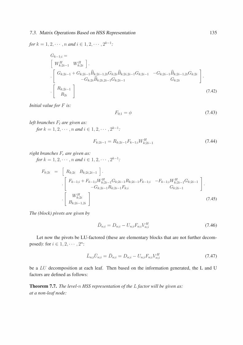
7.3. Matrix Operations Based on HSS Representation 135
for k = 1, 2, · · · , n and i ∈ 1, 2, · · · , 2k−1:
Gk−1;i =[
W Hk;2i−1 W H
k;2i
].
.
[Gk;2i−1 + Gk;2i−1Bk;2i−1,2iGk;2iBk;2i,2i−1Gk;2i−1 −Gk;2i−1Bk;2i−1,2iGk;2i
−Gk;2iBk;2i,2i−1Gk;2i−1 Gk;2i
].
.
[Rk;2i−1
R2i
](7.42)
Initial value for F is:
F0;1 = φ (7.43)
left branches Fℓ are given as:
for k = 1, 2, · · · , n and i ∈ 1, 2, · · · , 2k−1:
Fk;2i−1 = Rk;2i−1Fk−1;iWHk;2i−1 (7.44)
right branches Fr are given as:
for k = 1, 2, · · · , n and i ∈ 1, 2, · · · , 2k−1:
Fk;2i =[
Rk;2i Bk;2i,2i−1
].
.
[Fk−1;i + Fk−1;iW
Hk;2i−1Gk;2i−1Rk;2i−1Fk−1;i −Fk−1;iW
Hk;2i−1Gk;2i−1
−Gk;2i−1Rk;2i−1Fk;i Gk;2i−1
].
.
[W H
k;2i
Bk;2i−1,2i
](7.45)
The (block) pivots are given by
Dn;i = Dn;i − Un;iFn;iVHn;i (7.46)
Let now the pivots be LU-factored (these are elementary blocks that are not further decom-
posed): for i ∈ 1, 2, · · · , 2n:
Ln;iUn;i = Dn;i = Dn;i − Un;iFn;iVHn;i (7.47)
be a LU decomposition at each leaf. Then based on the information generated, the L and U
factors are defined as follows:
Theorem 7.7. The level-n HSS representation of the L factor will be given as:
at a non-leaf node:

136 Chapter 7. Algorithms to Solve Hierarchically Semi-separable Systems
for k = 1, 2, · · · , n; i ∈ 1, 2, · · · , 2k−1 and j = 1, 2, · · · , 2k:
Rk;j = Rk;j Wk;2i−1 = Wk;2i−1
W Hk;2i = W H
k;2i − W Hk;2i−1Gk;2i−1Bk;2i−1,2i
Bk;2i,2i−1 = Bk;2i,2i−1 Bk;2i−1,2i = 0
(7.48)
at a leaf:
for i ∈ 1, 2, · · · , 2n:
Un;i = Un;i Vn;i = U−Hn;i Vn;i D = Ln;i (7.49)
Theorem 7.8. The level-n HSS representation of the U factor will be given as:
at a non-leaf node:
for k = 1, 2, · · · , n; i ∈ 1, 2, · · · , 2k−1 and j = 1, 2, · · · , 2k:
Rk;2i−1 = Rk;2i−1 Rk;2i = Rk;2i − Bk;2i,2i−1Gk;2i−1Rk;2i−1 Wk;j = Wk;j
Bk;2i,2i−1 = 0 Bk;2i−1,2i = Bk;2i−1,2i
(7.50)
at a leaf:
for i ∈ 1, 2, · · · , 2n:
Un;i = L−1n;iUn;i Vn;i = Vn;i Dn;i = Un;i (7.51)
Proof for the Traverse
We start with the proof of theorem 7.6. Given the updating operations on G and downdating
operations on F accounted for in the introductory part of this section, it remains to verify that
there exists a recursive order to compute all the quantities indicated. Initialization results in the
Fk,1 = φ for all k = 1 · · ·n. In particular, Fn,1 is now known, and Gn,1 can be computed. This
in turn allows for the computation of Fn,2 thanks to the Fr downdate formula at level (k − 1, 1).
Now Gn,2 can be computed, and next the first left bottom node Gn−1,1 is dealt with. We now
dispose of enough information to compute Fn−1,2, since Gn−1,1 and Fn−2,1 = φ are known (this
being the beginning of the next step).
The general dependencies in the formulas are as follows. At a leaf: Gn;i depends on Fn;i; at a
non-leaf node: Gk−1,i is dependent on Gk,2i−1 and Gk,2i; Fk;2i−1 is dependent on Fk−1,i and Fk,2i
is dependent on both Fk−1,i and Gk,2i−1. Considering the closure of data dependencies, the full
dependencies at a node are given in Figure 7.3. With the F matrices on the root initialized, the or-
der in which all the F and G quantities can be computed on a node is Fk−1;i → Fk;2i−1 → Gk;2i−1
→ Fk;2i → Gk;2i → Gk−1;i, or equivalently parent→left children→right children→parent. That
is: with a post-order traverse on the binary tree (note that: the F on the root is initialized), all
unknown F s and Gs can be filled in.

7.3. Matrix Operations Based on HSS Representation 137
Figure 7.3: The dependencies of the intermediate variables on one no-leaf node
Figure 7.4: The computation of Fk;2i with the help of Fk−1;i and Gk;2i−1
Proof of the Formulas for L and U Factors
Let now the pivots be LU-factored (these are elementary blocks that are not further decomposed).
We may assume that at each step the Schur complements have been computed and updated. To
get the L and U factors recursively as in formula (7.31), it is obvious that for each leaf of the
L factor, D = L, U = U , V H = V Hl U−1; for each leaf of the U factor, D = U, U = L−1U ,
V = V .
For all left branches, the blocks are updated by modifying B matrices with formula (7.41) to
compute the Schur complement Dk;i = Dk;i − Un;iFn;iVHn;i. But for the right branches, updating
B matrices with formula (7.41) is not enough because Fk−1;i only subsumes the information
from its parent. Its left sibling has to be taken into consideration for the update of the Schur
complement.
Assuming the correct update has been done for the DA block and Dℓ block (see Figure 7.4),
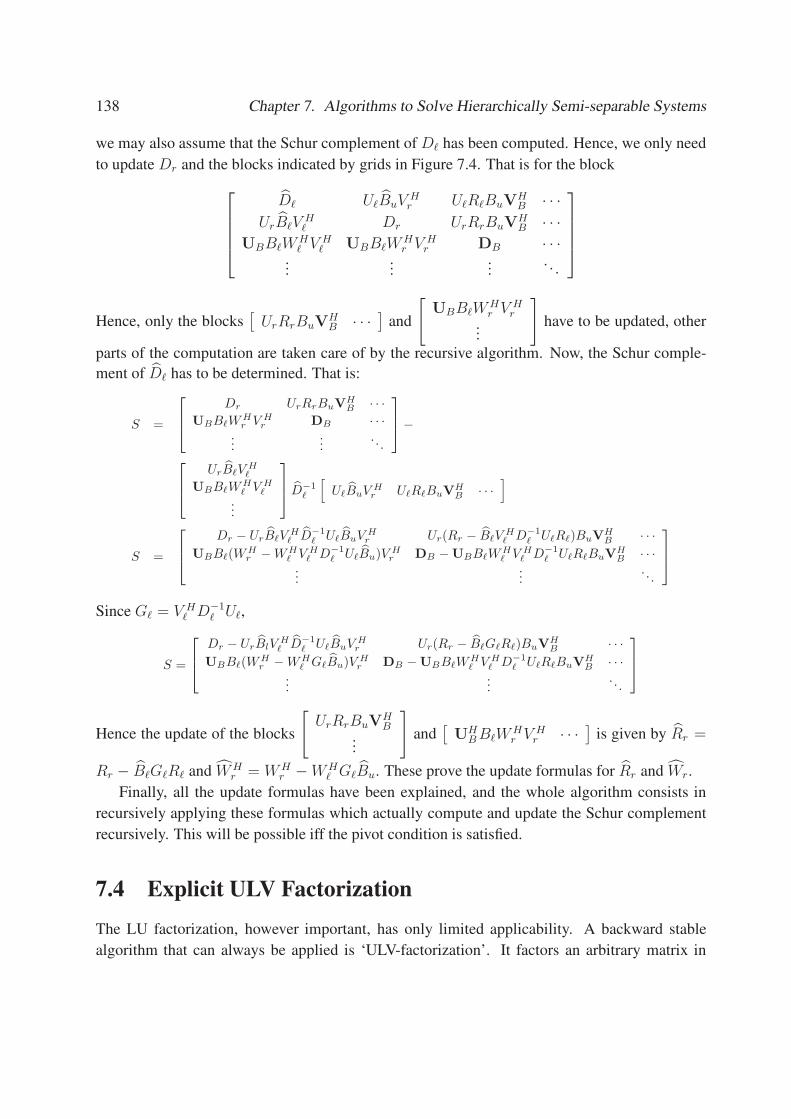
138 Chapter 7. Algorithms to Solve Hierarchically Semi-separable Systems
we may also assume that the Schur complement of Dℓ has been computed. Hence, we only need
to update Dr and the blocks indicated by grids in Figure 7.4. That is for the block
Dℓ UℓBuVHr UℓRℓBuV
HB · · ·
UrBℓVHℓ Dr UrRrBuV
HB · · ·
UBBℓWHℓ V H
ℓ UBBℓWHr V H
r DB · · ·...
......
. . .
Hence, only the blocks[
UrRrBuVHB · · ·
]and
[UBBℓW
Hr V H
r...
]have to be updated, other
parts of the computation are taken care of by the recursive algorithm. Now, the Schur comple-
ment of Dℓ has to be determined. That is:
S =
Dr UrRrBuVH
B· · ·
UBBℓWHr V H
r DB · · ·...
.... . .
−
UrBℓVH
ℓ
UBBℓWH
ℓV H
ℓ
...
D−1
ℓ
[UℓBuV H
r UℓRℓBuVH
B· · ·
]
S =
Dr − UrBℓVH
ℓD−1
ℓUℓBuV H
r Ur(Rr − BℓVH
ℓD−1
ℓUℓRℓ)BuV
H
B· · ·
UBBℓ(WHr − WH
ℓV H
ℓD−1
ℓUℓBu)V H
r DB − UBBℓWH
ℓV H
ℓD−1
ℓUℓRℓBuV
H
B· · ·
......
. . .
Since Gℓ = V Hℓ D−1
ℓ Uℓ,
S =
Dr − UrBlVH
ℓD−1
ℓUℓBuV H
r Ur(Rr − BℓGℓRℓ)BuVH
B· · ·
UBBℓ(WHr − WH
ℓGℓBu)V H
r DB − UBBℓWH
ℓV H
ℓD−1
ℓUℓRℓBuV
H
B· · ·
......
. . .
Hence the update of the blocks
[UrRrBuV
HB
...
]and
[UH
B BℓWHr V H
r · · ·]is given by Rr =
Rr − BℓGℓRℓ and W Hr = W H
r − W Hℓ GℓBu. These prove the update formulas for Rr and Wr.
Finally, all the update formulas have been explained, and the whole algorithm consists in
recursively applying these formulas which actually compute and update the Schur complement
recursively. This will be possible iff the pivot condition is satisfied.
7.4 Explicit ULV Factorization
The LU factorization, however important, has only limited applicability. A backward stable
algorithm that can always be applied is ‘ULV-factorization’. It factors an arbitrary matrix in

7.4. Explicit ULV Factorization 139
three factors, a unitary matrix U , a (generalized) lower triangular L (a non-singular triangular
matrix embedded in a possibly larger zero matrix) and another unitary matrix V . In the present
section we show that the ULV-factorization for an HSS matrix of order n can be obtained in a
special form. Both U and V are again HSS, and the lower triangular factor L has a special HSS
form that is extremely sparse (many transfer matrices are zero). The ULV-factorization of A
leads directly to the Moore-Penrose inverse for A. One trims the L factor to its purely triangular
part, and the U and V factors to the corresponding relevant columns and rows to obtain the so
called ‘economic ULV factorization’ A = UeLeVe, the Moore-Penrose inverse then being given
as A† = V He L−1
e UHe . The determination of the inverse of a lower triangular HSS factor is treated
in the following section and gives rise to an HSS matrix of the same order and complexity. In
this thesis we follow the implicit ULV factorization method presented in [75], and show that the
implicit method can be made explicit with some non-trivial modifications. The Moore-Penrose
system can be then be solved with the explicit L factor. Alternatively one could follow the method
presented in [76] which has similar flavors, but uses a slightly different approach.
For the sake of definiteness and without impairing generality, we assume here that the HSS
matrix A has full row rank, and its n-level HSS representation is defined by the sequences
U, V, D, B, R, W . Similar to the implicit ULV factorization method, the explicit method in-
volves an upsweep recursion (or equivalently a post-order traverse). We start with the left-most
leaf. First, we treat the case in which the HSS representation, which will be recursively reduced,
has reached the situation given in equation (7.52). The second block row in that equation has a
central purely triangular blockAk;i of dimension δk;i, the goal will be to reduce the matrix further
by treating the next block row. Through the steps described in the following treatment this case
will be reached recursively by converting subtrees to leaves, so that the central compression step
always happens at the level of a leaf.
7.4.1 Treatment of a Leaf
The situation to be treated in this part of the recursion has the form
A =
. . . [...]V
(1)Hk;i [
...]V(2)Hk;i . .
.
0 Ak;i 0 0
Uk;i[· · · ] D(1)k;i D
(2)k;i Uk;i[· · · ]
. ..
[...]V
(1)Hk;i [
...]V(2)Hk;i
. . .
. (7.52)
It is assumed at this point that Ak;i is already lower triangular and invertible with dimension δk;i.
The next block row stands in line for treatment. The compression step attacks Uk;i. If Uk;i has
more rows than columns, it can be compressed by applying QL factorization on it:
Uk;i = Qk;i
[0
Uk;i
](7.53)

140 Chapter 7. Algorithms to Solve Hierarchically Semi-separable Systems
where Uk;i is square and has l rows. To keep consistence in the rows, we must apply QHk;i to Dk;i:
Dk;i = QHk;iDk;i. (7.54)
Assume that Dk;i has m columns. We can partition Dk;i as:
δk;i m − δk;i[D
(1)k;i D
(2)k;i
] = Dk;i (7.55)
Since Ak;i is already lower-triangular matrix, to proceed we only have to process the block D(2)k;i
so as to obtain a larger upper-triangular reduced block. Hence we LQ factorize D(2)k;i as:
D(2)k;i =
[D
(2)k;i;0,0 0
D(2)k;i;1,0 D
(2)k;i;1,1
]wk;i, (7.56)
where D(2)k;i;0,0 is lower triangular and has n columns;D
(2)k;i;1,0 and D
(2)k;i;1,1 have l rows. Now to
adjust the columns, we must apply wk;i on Vk;i. Let
δk;i
m − δk;i
[V
(1)k;i
V(2)k;i
]= Vk;i. (7.57)
Apply wk;i on V(2)k;i as
V(2)k;i = wk;iV
(2)k;i (7.58)
let: [D
(1,1)k;i
D(1,2)k;i
]= D
(1)k;i , (7.59)
where D(1,2)k;i has l rows. After these operations, the HSS representation has become
A =
. . . [...]V
(1)Hk;i [
...]V(21)Hk;i [
...]V(22)Hk;i . .
.
0 Ak;i 0 0 0
0 D(11)k;i D
(2)k;i;0,0 0 0
Uk;i[· · · ] D(1,2)k;i D
(2)k;i;1,0 D
(2)k;i;1,1 Uk;i[· · · ]
. ..
[...]V
(1)Hk;i [
...]V(21)Hk;i [
...]V(22)Hk;i
. . .
. (7.60)
The compressed leaf will be returned as:
Dk;i =[
D(1,2)k;i D
(2)k;i;1,0 D
(2)k;i;1,1
](7.61)
Uk;i = Uk;i (7.62)

7.4. Explicit ULV Factorization 141
Vk;i =
[V
(1)k;i
V(2)k;i
](7.63)
With
Ak;i =
[Ak;i 0
D(1,1)k;i D
(2)k;i;0,0
](7.64)
representing the reduced row slices, and
δk;i = δk;i + n (7.65)
Now, the commented HSS representation is exactly the same as the original, except the leaf has
become smaller. When Uk;i has more columns than rows, nothing can be done to compress in
this way. Then a new arrangement has to be created by merging two leaves into a new, integrated
leave. This process is treated in the next paragraph.
7.4.2 Merge
The behavior of this part of the algorithm on a leaf has been specified. If no leaf is available for
processing, one can be created by merging. Assume that we are at the node k; i, the algorithm
works in a post-order traverse way, it proceeds by first calling itself on the left children and
then on the right children. When the algorithm comes to the present stage, both the left and the
right child are already compressed leaves. They can then be merged by the following explicit
procedure.
Before the merge, the HSS representation is, in an obvious notation:
let
Y(1)k+1;2i−1;2i = Uk+1;2i−1Bk+1;2i−1;2iV
(1)Hk+1;2i
Y(2)k+1;2i−1;2i = Uk+1;2i−1Bk+1;2i−1;2iV
(2)Hk+1;2i
Y(1)k+1;2i;2i−1 = Uk+1;2iBk+1;2i;2i−1V
(1)Hk+1;2i−1
Y(2)k+1;2i;2i−1 = Uk+1;2iBk+1;2i;2i−1V
(2)Hk+1;2i−1
thus Dk;i can be represented as:
Dk;i =
Ak+1;2i−1 0 0 0
D(1)k+1;2i−1 D
(2)k+1;2i−1 Y
(1)k+1;2i−1;2i Y
(2)k+1;2i−1;2i
0 0 Ak+1;2i 0
Y(1)k+1;2i;2i−1 Y
(2)k+1;2i;2i−1 D
(1)k+1;2i D
(2)k+1;2i
(7.66)

142 Chapter 7. Algorithms to Solve Hierarchically Semi-separable Systems
Next, the rows and columns are moved to put all reduced rows on the top-left. After the reorder-
ing, the HSS representation becomes:
Dk;i =
Ak+1;2i−1 0 0 0
0 Ak+1;2i 0 0
D(1)k+1;2i−1 Y
(1)k+1;2i−1;2i D
(2)k+1;2i−1 Y
(2)k+1;2i−1;2i
Y(1)k+1;2i;2i−1 D
(1)k+1;2i Y
(2)k+1;2i;2i−1 D
(2)k+1;2i
(7.67)
and the merged leaf now has:
Dk;i =
[D
(1)k+1;2i−1 Y
(1)k+1;2i−1;2i D
(2)k+1;2i−1 Y
(2)k+1;2i−1;2i
Y(1)k+1;2i;2i−1 D
(1)k+1;2i Y
(2)k+1;2i;2i−1 D
(2)k+1;2i
](7.68)
Uk;i =
[Uk+1;2i−1Rk+1;2i−1
Uk+1;2iRk+1;2i
], Vk;i =
V(1)k+1;2i−1Wk+1;2i−1
V(1)k+1;2iWk+1;2i
V(2)k+1;2i−1Wk+1;2i−1
V(2)k+1;2iWk+1;2i−1
(7.69)
With the intermediate block
Ak;i =
[Ak+1;2i−1 0
0 Ak+1;2i
](7.70)
and
δk;i = δk+1;2i−1 + δk+1;2i (7.71)
Note that now the node has been reduced to a leaf, and the actual HSS system has two fewer
leaves. The compression algorithm can then be called on this leaf with Ak;i and δk;i.
7.4.3 Formal Algorithm
Having the above three procedures, we now describe the algorithm formally. Similar to the
implicit ULV factorization method, this algorithm is a tree-based recursive algorithm. It involves
a post-order traverse of the binary tree of the HSS representation. Let T be the root of the HSS
representation.
Function : post-order-traverse
Input: an actual HSS node or leaf T;
Output: a compressed HSS leaf)
1. (node, left-children, right-children) = T;
2. left-leaf = post-order-traverse left-child;

7.4. Explicit ULV Factorization 143
3. right-leaf = post-order-traverse right-child;
4. if left-child is compressible then
left-leaf = compress left-leaf;
else
do nothing;
5. if right-child is compressible then
right-leaf = compress right-leaf;
else
do nothing;
6. return compress (Merge(node,left-leaf,right-leaf));
Function : Explicit-ULV-Factorization
Input: a HSS representation T;
Output: the factor L in sparse matrix format
1. actual-T = T;
2. Leaf = post-order-traverse actual-T;
3. return Leaf.A0;1
Once the whole HSS tree is compressed as a leaf and the leaf is further compressed, the L
factor has been computed as L = A0;1.
7.4.4 Results
We show the result of the procedure applied to an HSS matrix A of dimensions 500 × 700 with
full row rank. Its HSS representation is of 5 levels deep and balanced. We apply the explicit
ULV factorization algorithm on it. Then the sparsity pattern of the L factor will be as in Figure
7.5. L has 500 rows and 700 columns. Its sparsity is 3.08% (The sparsity depends on the HSS
complexity, the lower the complexity is, the sparser the L factor is.). With the assumption that A
has full row rank, The non-zero block of L is square and invertible.
7.4.5 Remarks
• Assume A has full column rank, the algorithm above can be modified to produce the URV
factorization (by compressing Vk;i instead of Uk;i).
• The explicit factor shall be kept in sparse matrix form.

144 Chapter 7. Algorithms to Solve Hierarchically Semi-separable Systems
Figure 7.5: The Sparsity pattern of L factor of the explicit ULV factorization
• the U and V factors are kept in an implicit form. This is convenient because they can be
easily applied to b and x when solve the system Ax = b.
• The complexity is higher than the implicit ULV factorization method, but it shall still be
linear. It can also be easily be seen that the HSS complexity of the result is the same as of
the original (with many transfer matrices reduced to zero).
7.5 Inverse of Triangular HSS Matrix
In this section, we will show how a triangular HSS matrix can be inverted efficiently. We shall
only present our fast inverse algorithm on upper triangular HSS matrices, since the algorithm
for lower triangular matrices is dual and similar. With the combination of the LU factorization
algorithm, the inverse algorithm for triangular systems and the matrix-matrix multiplication algo-
rithm, the HSS inverse of a square invertible HSS matrix, of which all block pivots are invertible,
can be computed.
Let the level-n HSS representation of the upper triangular matrix A be given by the sequence
of R, W , B, U , V and D (where the D’s are upper triangular). Assuming all D matrices invert-
ible, the level-n HSS representation of the inverse of A is given by R, W , B, U , V and D (where
Ds are again upper triangular) with the formulas given below. We use the following (trivial) fact
recursively.

7.5. Inverse of Triangular HSS Matrix 145
Lemma 1. The inverse of Dk−1;⌈ i2⌉ (i is a odd number) is given by
D−1k−1;⌈ i
2⌉
=
[Dk;i Uk;iBk;i,i+1V
Hk;i+1
0 Dk;i+1
]−1
=
[D−1
k;i −D−1k;i Uk;iBk;i,i+1V
Hk;i+1D
−1k;i+1
0 D−1k;i+1
](7.72)
We have
Uk;i =
[Dk+1;2i−1 Uk+1;2i−1Bk+1;2i−1,2iV
Hk+1;2i
0 Dk+1;2i
]−1
Uk;i
Uk;i =
[Dk+1;2i−1 Uk+1;2i−1Bk+1;2i−1,2iV
Hk+1;2i
0 Dk+1;2i
]−1
.
.
[Uk+1;2i−1Rk+1;2i−1
Uk+1;2iRk+1;2i
]
Uk;i =
[D−1
k+1;2i−1 −D−1k+1;2i−1Uk+1;2i−1Bk+1;2i−1,2iV
Hk+1;2iD
−1k+1;2i
0 D−1k+1;2i
].
.
[Uk+1;2i−1Rk+1;2i−1
Uk+1;2iRk+1;2i
]
Uk;i =
[D−1
k+1;2i−1Uk+1;2i−1(Rk+1;2i−1 − Bk+1;2i−1,2iVHk+1;2iD
−1k+1;2iUk+1;2iRk+1;2i)
D−1k+1;2iUk+1;2iRk+1;2i
]
Assuming that Uk+1;2i−1 and Uk+1;2i have been updated asD−1k+1;2i−1 Uk+1;2i−1 andD−1
k+1;2iUk+1;2i;
the update for Uk;i follows from the update Rk+1;2i−1 as
Rk+1;2i−1 = Rk+1;2i−1 − Bk+1;2i−1,2iVHk+1;2iU
−1k+1;2iUk+1;2iRk+1;2i (7.73)
The formulas for Vk;i+1 become
V Hk;i+1 = V H
k;i+1
[Dk+1;2i+1 Uk+1;2i+1Bk+1;2i+1,2i+2V
Hk+1;2i+2
0 Dk+1;2i+2
]−1
V Hk;i+1 =
[W H
k+1;2i+1VHk+1;2i+1 W H
k+1;2i+2VHk+1;2i+2
].
.
[Dk+1;2i+1 Uk+1;2i+1Bk+1;2i+1,2i+2V
Hk+1;2i+2
0 Dk+1;2i+2
]−1
V Hk;i+1 =
[W H
k+1;2i+1VHk+1;2i+1 W H
k+1;2i+2VHk+1;2i+2
].
.
[D−1
k+1;2i+1 −D−1k+1;2i+1Uk+1;2i+1Bk+1;2i+1,2i+2V
Hk+1;2i+2D
−1k+1;2i+2
0 D−1k+1;2i+2
]

146 Chapter 7. Algorithms to Solve Hierarchically Semi-separable Systems
let
W Hk+1;2i+2 = W H
k+1;2i+2 − W Hk+1;2i+1V
Hk+1;2i+1D
−1k+1;2i+1Uk+1;2i+1Bk+1;2i+1,2i+2
then
V Hk;i+1 =
[W H
k+1;2i+1VHk+1;2i+1D
−1k+1;2i+1 W H
k+1;2i+2VHk+1;2i+2D
−1k+1;2i+2
]
Assuming now that V Hk+1;2i+1 and V H
k+1;2i+2 have been updated as V Hk+1;2i+1D
−1k+1;2i+1 and
V Hk+1;2i+2D
−1k+1;2i+2, the update for Vk;i+1 follows from
W Hk+1;2i+2 = W H
k+1;2i+2 − W Hk+1;2i+1V
Hk+1;2i+1D
−1k+1;2i+1Uk+1;2i+1Bk+1;2i+1,2i+2 (7.74)
next the update for −Uk;iBk;i,jVHk;j follows from
Bk;i,j = −Bk;i,j (7.75)
Let the intermediate G be defined as Gk;i = V Hk;iD
−1k;i Uk;i, then the above update formulas can be
written as
W Hk;2i = W H
k;2i − W Hk;2i−1Gk;2i−1Bk;2i−1,2i
Wk;2i−1 = Wk;2i−1
Rk;2i−1 = Rk;2i−1 − Bk;2i−1,2iGk;2iRk;2i
Rk;2i = Rk;2i
Bk;i,j = −Bk;i,j
(7.76)
The recursive formula for the intermediate variable G is as follows. According to the definition
of Gk−1;i:
Gk−1;i =[
W Hk;2i−1V
Hk;2i−1 W H
k;2i−1VHk;2i
].
.
[Dk;2i−1 Uk;2i−1Bk;2i−1,2iV
Hk;2i
0 Dk;2i
]−1 [Uk;2i−1Rk;2i−1
Uk;2iRk;2i
]
Gk−1;i =[
W Hk;2i−1V
Hk;2i−1 W H
k;2i−1VHk;2i
].
.
[D−1
k;2i−1 −D−1k;2i−1Uk;2i−1Bk;2i−1,2iV
Hk;2iD
−1k;2i
0 D−1k;2i
][Uk;2i−1Rk;2i−1
Uk;2iRk;2i
]
Gk−1;i =[
W Hk;2i−1 W H
k;2i−1
].
.
[V H
k;2i−1D−1k;2i−1Uk;2i−1 −V H
k;2i−1D−1k;2i−1Uk;2i−1Bk;2i−1,2iV
Hk;2iD
−1k;2iUk;2i
0 V Hk;2iD
−1k;2iUk;2i
].
.
[Rk;2i−1
Rk;2i
]
Gk−1;i =[
W Hk;2i−1 W H
k;2i−1
] [ Gk;2i−1 −Gk;2i−1Bk;2i−1,2iGk;2i
0 Gk;2i
][Rk;2i−1
Rk;2i
]
Summarizing

7.6. Ancillary Operations 147
Definition 7.5. Let the intermediate variable G be defined as
for k = 1, 2, · · · , n and i ∈ 1, 2, · · · , 2k−1:
Gk;i = V Hk;iD
−1k;i Uk;i (7.77)
The upsweep recursion for G is:
Gk−1;i =[
W Hk;2i−1 W H
k;2i
] [ Gk;2i−1 −Gk;2i−1Bk;2i−1,2iGk;2i
0 Gk;2i
] [Rk;2i−1
Rk;2i
](7.78)
and hence
Theorem 7.9. The level-n HSS representation of the inverse of the upper triangular HSS matrix
is given by the following sequence of operations
for k = 1, 2, · · · , n; j ∈ 1, 2, · · · , 2k and i ∈ 1, 2, · · · , 2k−1:
W Hk;2i = W H
k;2i − W Hk;2i−1Gk;2i−1Bk;2i−1,2i Wk;2i−1 = Wk;2i−1
Rk;2i−1 = Rk;2i−1 − Bk;2i−1,2iGk;2iRk;2i Rk;2i = Rk;2i
Bk;2i−1,2i = −Bk;2i−1,2i Bk;2i,2i−1 = 0
Uk;j = D−1k;jUk;j V H
k;j = V Hk;jD
−1k;j
DHk;j = D−1
k;j
(7.79)
7.6 Ancillary Operations
In this section, we will discuss various ancillary operations that help to (re-) construct an HSS
representation in various circumstances. These operations will help to reduce the HSS complex-
ity or to keep the column base and row base dependencies of the HSS representation.
7.6.1 Column (row) Base Insertion
When the off-diagonal blocks have to be changed at the nodes at a higher level, column bases
and row bases may have to be changed. To keep the column and row base dependencies, new
column (row) bases may have to be added to the lower levels. We might be able to generate
these bases from the column (row) bases of the lower level nodes, but this is not guaranteed.
Taking a conservative approach we insert column (row) bases into the lower level and then do
compression to reduce the complexity of the HSS representation.
The algorithm combines two sub-algorithms (downsweep base insertion and then a compres-
sion). The compression procedure is used to eliminate redundant bases and reduce the HSS
complexity. Compression does not have to be done after every downsweep column (row) base
insertion. To save the computation cost, we may do one step of compression after a number of
steps of bases insertion.
We will present row base insertion in details, while column base insertion is dual and hence
similar.

148 Chapter 7. Algorithms to Solve Hierarchically Semi-separable Systems
Downsweep Row Base Insertion
Suppose that we need to add a row base represented by a conformal matrix v to an HSS node
A without changing the matrix it represents (the column dimension of v should of course be
conformal to the row dimension of A.) Let the original HSS node be represented as
[D1;1 U1;1B1;1,2V
H1;2
U1;2B1;2,1VH1;1 D1;2
.
]
The algorithm works in a downsweep fashion modifying the nodes and leaves in the HSS tree.
• Row base insertion at a non-leaf node
vk;i is split according to the column partition of A at this node:
for k = 1, 2, · · · , n and i ∈ 1, 2, · · · , 2k:
vk;i =
[vk+1;2i−1
vk+1;2i
]
vk+1;2i−1 is inserted to the left child, vk+1;2i to the right child recursively. vk+1;2i−1 can
be generated from Dk+1;2i−1, and vk+1;2i from Dk+1;2i. The translation matrices of this
node must be modified to make sure that the base insertion does not change the matrix it
represents as follows
for k = 1, 2, · · · , n; i ∈ 1, 2, · · · , 2k, and j = i + 1 for odd i, j = i − 1 for even i:
Wk;i =
[Wk;i 0
0 I
]
Bk;i,j =[
Bk;i,j 0] . (7.80)
• Row base insertion at a leaf
a leaf is reached by recursion, vn;i has to be inserted to the leaf, hence
for k = 1, 2, · · · , n and i ∈ 1, 2, · · · , 2k:
Vn;i =[
Vn;i vn;i
](7.81)
Compression
After applying downsweep base insertion to A, the row bases v required by the upper level can
be generated from A. But the HSS representation we get may have become redundant.
Since only the row base has been modified, we only have to factor Vn;i matrices as
for k = 1, 2, · · · , n and i ∈ 1, 2, · · · , 2k:
Vn;i = Vn;iwn;i (7.82)

7.6. Ancillary Operations 149
This should be done by a rank revealing QR or QL factorization, then Vn;i will be column or-
thonormal (and it will surely be column independent). The factor wn;i will then be propagated to
the upper level, where the translation matrices Bn;i,j and Wn;i will be modified by the factor w
as follows
for k = 1, 2, · · · , n; i ∈ 1, 2, · · · , 2k, and j = i + 1 for odd i, j = i − 1 for even i:
Bk;i,j = Bk;i,jwHk;j
Wk;i = wk;iWk;i
Rk;i = Rk;i
(7.83)
Then we do compression on the higher level. Since only row bases have been modified, we only
have to factor [Wk;2i−1
Wk;2i
]=
[Wk;2i−1
Wk;2i
]wk−1;i (7.84)
Note that Wk;2i−1 and Wk;2i have been modified by the wk;2i−1 and wk;2i factors coming from its
children with the formulas (7.83), the factorization should again be rank-revealing. The wk−1;i
factor will then be propagated further to the upper level, and the algorithm proceeds recursively.
After applying the whole algorithm to the a HSS node, the new row base vH will be inserted
by appending it to the original row base. Suppose the row base of the original node is given by
V H , the modified node becomes[
V v]H
. Note that base insertion does not change the HSS
matrix, it only modifies its HSS representation.
Column Base Insertion
The algorithm for column base insertion is similar and dual to the one for row base insertion.
Modifications will now be done on U , R instead of V , W . The B matrices will be modified
as Bk;i,j =
[Bk;i,j
0
]instead of
[Bk;i,j 0
]After applying the row bases insertion to a HSS
node, the new column bases will be appended after its original column bases. The compression
algorithm for column base insertion should also be modified accordingly.
7.6.2 Append a Matrix to a HSS Matrix
This algorithm appends a thin slice C to a HSS matrix A. This operation is central in the Moore-
Penrose HSS inversion treated in [76]. We establish that the result of this operation will still be
HSS matrix whose HSS representation can be computed easily. Obviously, we may append the
matrix to the top of the HSS matrix, to the left of the HSS matrix, to the right of the HSS matrix
or to the bottom of the HSS matrix. Here we just present the method to append matrix to the left
of the HSS matrix. Others can be easily derived mutatis mutandis.

150 Chapter 7. Algorithms to Solve Hierarchically Semi-separable Systems
Append a rank-k matrix to a HSS matrix
Suppose
A =[
C A]
(7.85)
Matrix B should have the same number of rows as A does, A is HSS matrix whose HSS repre-
sentation is defined by the sequences UA, VA, DA, RA,WA and BA.
Instead of trying to absorb the C matrix into the HSS representation of A matrix, we rewrite
the formula (7.85) as:
A =
[ − −C A
](7.86)
where − is a dummy matrix which has no rows. A is an HSS matrix which has one more level
than A does.
We then assume that C = UBV H . That is: C is a rank-k matrix. The decomposition of C
can be computed by a URV factorization or SV D factorization (in practice, we normally have
its decomposition already available).
Then the column base U of C shall be inserted to the HSS representation of A so that U can
be generated from the HSS representation of A. This can be done in many different ways. The
most straightforward is to insert the column base using the algorithm described in Section 7.6.1
and followed by a step of compression depending on how many columns U has. Suppose that
after column bases insertion, the HSS representation of A becomes A. (Note that: column bases
insertion does not change the HSS matrix, it only changes the HSS representation.)
Then A will be represented as
A =
[ − −UBV H A
](7.87)
It is easy to check that the HSS representation of A will be given as
at the top node B1;1,2 = ∅ B1;2,1 = B W1;1 = |W1;2 = ∅ R1;1 = ∅ R1;2 = | (7.88)
at the left branch:
D1;1 = − U1;1 = ∅ V1;1 = V (7.89)
at the right branch:
D1;2 = A (7.90)
where | and − represent dummy matrices with no columns respect. no rows. ∅ represents the
dummy matrix without column or or row. The other dimensions of all these should be correct
such that the HSS representation is still valid.

7.7. Complexity Analysis 151
Matrix-Append when Bases are Semi-Separable
In practice, we almost never compute U and V , since these computations are costly and break
the idea of the HSS representation. For instance, when a matrix UBV H needs to be appended to
a HSS matrix A, U and V are not explicitly stored. They are defined by the formulas (7.10) and
(7.11).
In this case, the formulas in the last subsection will have to be modified accordingly, The left
branch of A will not be of just one level. Instead, the left child will be a sub-HSS tree defined by
the following sequences:
at the root: B1;1,2 = ∅ B1;2,1 = B W1;1 = |W1;2 = ∅ R1;1 = ∅ R1;2 = | (7.91)
at non-leaf nodes:
for k = 2, 3, · · · , n and i ∈ 1, 2, · · · , 2k−1:
Rk;2i−1 = | Rk;2i = | Bk;2i−1,2i = −Bk;2i,2i−1 = − Wk;2i−1 = Wk;2i−1 Wk;2i = Wk;2i
(7.92)
at the leaves:
Un;i = ∅ Vn;i = Vn;i Dn;i = − (7.93)
note that since the column base U is also in a hierarchically semi-separable form, inserting it into
A will be somewhat different than that in Section (7.6.1). The modified formulas for inserting a
column base U to A are given by
for k = 1, 2, · · · , n; i ∈ 1, 2, · · · , 2k−1; j = i + 1 for odd i and j = i − 1 for even i:
Bk;i,j =
[BA;k;i,j
0
]
Rk;i =
[RA;k;i 0
0 Rk;i
]
Uk;i =[
UA;k;i Uk;i
]
(7.94)
7.7 Complexity Analysis
From the algorithms given, the time complexity of the elementary operations can easily be eval-
uated together with their effect on the representation complexity of the resulting HSS structure.
The same matrix can be represented by many different HSS representations, in which some are
better than others in terms of computation complexity and space complexity. The HSS represen-
tation complexity should be defined in such a way that operations on the HSS representation with
higher HSS representation complexity cost more time and memory than those on HSS represen-
tations with lower HSS representation complexity. Many indicators can be used. Here, we use a
rough measure for the HSS representation complexity as follows

152 Chapter 7. Algorithms to Solve Hierarchically Semi-separable Systems
Definition 7.6. HSS complexity: the total number of free entries in the HSS representation.
Definition 7.7. Free entries: free entries are the entries which can be changed without restriction
(For instance, the number of free entries in n × n diagonal matrix will be n, that in n × n
triangular matrix will be n(n − 1)/2...etc).
The HSS complexity actually indicates the least possible memory needed to store the HSS
representation. It also implies the computation complexity, assuming each free entry is accessed
once or a small number of times during operations (we may have to account for intermediary
representations as well).
Since most of the algorithms given are not so complicated and some have been studied in the
literature, we shall limit ourselves to listing a summarizing table for the existing HSS algorithms
(including some from the literature). We assume that n is the dimension of the HSS matrix and
k is the maximum rank of the translation matrices (more accurate formulas can be derived when
more detailed information on local rank is available). Table 7.1 gives a measure of the numerical
complexity in terms of n and k, as well as an indication of the HSS complexity of the resulting
structure.
We see that in all cases the complexity is linear in the original size of the matrix, and a to be
expected power of the size of the translation matrices. Of course, a much more detailed analysis
is possible but falls beyond the scope of this thesis.
7.8 Connection between SSS, HSS and the Time Varying No-
tation
In the earlier papers on SSS [77, 44], efficient algorithms have been developed. Although differ-
ent algorithms have to be used corresponding to these two seemingly different representations,
we would like to show that they are not so different, and we will show how they can be converted
to each other. By converting between these two representations, we can take advantages of the
fast algorithms for these two different representations.
7.8.1 From SSS to HSS
In [44], the SSS representation for A is defined as follows: let A be an N × N matrix satisfying
the SSS matrix structure. Then there exist n positive integers m1, ...mn with N = m1 + ...mn to
block-partition A as A = Ai,j, where Aij ∈ Cmi×mj satisfies
Aij =
Di if i = j
UiWi+1...Wj−1VHj if j > i
PiRi−1...Rj+1QHj if j < i
(7.95)
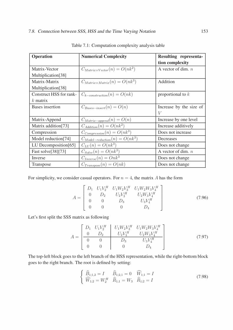
7.8. Connection between SSS, HSS and the Time Varying Notation 153
Table 7.1: Computation complexity analysis table
Operation Numerical Complexity Resulting representa-
tion complexity
Matrix-Vector
Multiplication[38]
CMatrix×V ector(n) = O(nk2) A vector of dim. n
Matrix-Matrix
Multiplication[38]
CMatrix×Matrix(n) = O(nk3) Addition
Construct HSS for rank-
k matrix
Ck−construction(n) = O(nk) proportional to k
Bases insertion CBases−insert(n) = O(n) Increase by the size of
V
Matrix-Append CMatrix−append(n) = O(n) Increase by one level
Matrix addition[73] CAddition(n) = O(nk2) Increase additively
Compression CCompression(n) = O(nk3) Does not increase
Model reduction[74] CModel−reduction(n) = O(nk3) Decreases
LU Decomposition[65] CLU(n) = O(nk3) Does not change
Fast solve[38][73] CSolve(n) = O(nk3) A vector of dim. n
Inverse CInverse(n) = Onk3 Does not change
Transpose CTranspose(n) = O(nk) Does not change
For simplicity, we consider casual operators. For n = 4, the matrix A has the form
A =
D1 U1VH2 U1W2V
H3 U1W2W3V
H4
0 D2 U2VH3 U2W3V
H4
0 0 D3 U3VH4
0 0 0 D4
(7.96)
Let’s first split the SSS matrix as following
A =
D1 U1VH2 U1W2V
H3 U1W2W3V
H4
0 D2 U2VH3 U2W3V
H4
0 0 D3 U3VH4
0 0 0 D4
(7.97)
The top-left block goes to the left branch of the HSS representation, while the right-bottom block
goes to the right branch. The root is defined by setting:
B1;1,2 = I B1;2,1 = 0 W1;1 = I
W1;2 = W H2 R1;1 = W3 R1;2 = I
(7.98)

154 Chapter 7. Algorithms to Solve Hierarchically Semi-separable Systems
Then we construct the left branch with a similar partitioning.
[D1 U1V
H2
0 D2
](7.99)
hence
D2;1 = D1 U2;1 = U1 V2;1 = V1 (7.100)
while for the right child
D2;2 = D2 U2;2 = U2 V2;2 = V2 (7.101)
In order to keep the HSS representation valid, R and W matrices on the left node should be set
properly. That is R2;1 = W2 R2;2 = I W2;1 = I
W2;2 = W H1 B2;2,1 = 0 B2;1,2 = I
(7.102)
and similarly for the right branch with partitioning as in (7.99)
D2;3 = D3 U2;3 = U3 V2;3 = V3 , (7.103)
D2;4 = D4 U2;3 = U4 V2;4 = V4 (7.104)
In order to keep the HSS representation valid, R and W matrices on the right node should be set
properly. That is R2;3 = W4 R2;4 = I W2;3 = I
W2;4 = W H3 B2;4,3 = 0 B2;3,4 = I
(7.105)
Finally the HSS representation can be written as:
A =
D2;1 U2;1B2;1,2VH2;2 U2;1R2;1B1;1,2W
H2;3V
H2;3 U2;1R2;1B1;1,2W
H2;4V
H2;4
0 D2;2 U2;2R2;2B1;1,2WH2;3V
H2;3 U2;2R2;2B1;1,2W
H2;4V
H2;4
0 0 D2;3 U2;3B2;3,4VH2;4
0 0 0 D2;4
(7.106)
with all the translation matrices set in equation (7.98) to (7.105).
The general transformation is then as follows. First we must partition the SSS matrix accord-
ing to a certain hierarchical partitioning. Then for a current HSS node at k level which should
contain the SSS blocks Axy where i ≤ x, y ≤ j (1 ≤ i < j ≤ n) and assuming the HSS block
is further partitioned at block h (i < h < j) the translation matrices of the current node can be
chosen as Bk;2i−1,2i = I Bk;2i,2i−1 = 0 Wk;2i−1 = I
Wk;2i =∏i
x=h W Hx Rk;2i−1 =
∏jx=h+1 Wx Rk;2i = I
(7.107)

7.8. Connection between SSS, HSS and the Time Varying Notation 155
Figure 7.6: HSS partitioning (on the left), SSS partitioning (on the right)
note that undefined Wx matrices are set equal I (the dimension of I is defined according to
context). If i = h or h + 1 = j, then one (or two) HSS leaf (leaves) have to be constructed by
letting
Dk;i = Dh Uk;i = Uh Vk;i = Vh (7.108)
After the HSS node of the current level has been constructed, the same algorithm is applied
recursively to construct the HSS node for SSS blocks Axy, i ≤ x, y ≤ h and for SSS block
Axy, h + 1 ≤ x, y ≤ j (the recursion stops when a leaf is constructed.).
Observing the fact that all Bk;2i,2i−1 matrices are zeros matrices and Wk;2i−1, Rk;2i−1 are
identity matrices, modifications can be done to get a more efficient HSS representation.
7.8.2 From HSS to SSS
In this section, we shall consider HSS as recursive SSS using the concise time-varying notation of
[39]. We shall first illustrate the algorithm by an example on 8×8 HSS representation. Different
partitioning are possible, e.g. those illustrated in Figure 7.8.2.
We shall only consider the upper triangular case, as that is the standard case in time-varying
system theory. The 4-level balanced HSS representation can be expanded as:
A =
D1;1 U1;1B1;1,2WH2;3V
H2;3 U1;1B1;1,2W
H2;4W
H3;7V
H3;7 U1;1B1;1,2W
H2;4W
H3;8V
H3;8
0 D2,3 U2;3B2;3,4WH3;7V
H3;7 U2;3B2;3,4W
H3;8V
H3;8
0 0 D3;7 U3;7B3;7,8VH3;8
0 0 0 D3;8
(7.109)
This has to be converted to the time-varying representation for k = 4:
A =
D1 B1C2 B1A2C3 B1A2A3C4
0 D2 B2C3 B2A3C4
0 0 D3 B3C4
0 0 0 D4
(7.110)
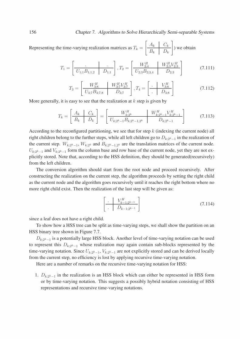
156 Chapter 7. Algorithms to Solve Hierarchically Semi-separable Systems
Representing the time-varying realization matrices as Tk =
[Ak Ck
Bk Dk
]) we obtain
T1 =
[. .
U1;1B1;1,2 D1;1
], T2 =
[W H
2;4 W H2;3V
H2;3
U2;3B2;3,4 D2;3
](7.111)
T3 =
[W H
3;8 W H3;7V
H3;7
U3;7B3;7,8 D3;7
], T4 =
[. V H
3;8
. D3;8
](7.112)
More generally, it is easy to see that the realization at k step is given by
Tk =
[Ak Ck
Bk Dk
]=
[W H
k;2k W Hk;2k−1
V Hk;2k−1
Uk;2k−1Bk;2k−1,2k Dk;2k−1
](7.113)
According to the reconfigured partitioning, we see that for step k (indexing the current node) all
right children belong to the further steps, while all left children go to Dk;2k−1 in the realization of
the current step. Wk;2k−1, Wk;2k and Bk;2k−1,2k are the translation matrices of the current node.
Uk;2k−1 and Vk;2k−1 form the column base and row base of the current node, yet they are not ex-
plicitly stored. Note that, according to the HSS definition, they should be generated(recursively)
from the left children.
The conversion algorithm should start from the root node and proceed recursively. After
constructing the realization on the current step, the algorithm proceeds by setting the right child
as the current node and the algorithm goes recursively until it reaches the right bottom where no
more right child exist. Then the realization of the last step will be given as:
[. V H
k−1;2k−1
. Dk−1;2k−1
](7.114)
since a leaf does not have a right child.
To show how a HSS tree can be split as time-varying steps, we shall show the partition on an
HSS binary tree shown in Figure 7.7.
Dk;2k−1 is a potentially large HSS block. Another level of time-varying notation can be used
to represent this Dk;2k−1 whose realization may again contain sub-blocks represented by the
time-varying notation. Since Uk;2k−1, Vk;2k−1 are not explicitly stored and can be derived locally
from the current step, no efficiency is lost by applying recursive time-varying notation.
Here are a number of remarks on the recursive time-varying notation for HSS:
1. Dk;2k−1 in the realization is an HSS block which can either be represented in HSS form
or by time-varying notation. This suggests a possibly hybrid notation consisting of HSS
representations and recursive time-varying notations.

7.9. Design of the HSS Iterative Solver 157
Figure 7.7: Binary tree partitioning
2. Uk;2k−1 and Vk;2k−1 form HSS bases generated from Dk;2k−1. For this recursive time-
varying notation, they should not be explicitly stored and can be derived locally in the
current step.
3. It is possible to represent general HSS matrices (not just block upper-triangular matrices)
with the recursive time-varying notation.
4. All fast HSS algorithms can be interpreted in a recursive time-varying fashion.
5. Some algorithms applied on time-varying notation described in [39] can be extended to the
recursive time-varying notation (HSS representation).
7.9 Design of the HSS Iterative Solver
Practical iterative solvers consist of standard iterative solutionmethods (CG, CGS, GMRES, etc),
appropriate preconditioners, efficient matrix-vector multiplicationmethods, and accurate conver-
gence estimation. We have implemented some iterative algorithms with OCAML and camlfloat
[78]. For the Krylov space iterative solvers, we have implemented solvers like CG, CGS, BiCG,
Bi-CGSTAB and so on (all based on the HSS representation). With all the algorithms under the
HSS framework, it is quite easy to combine the HSS representation and its fast algorithms with
any iterative solution methods.
7.9.1 Preconditioners
As well studied by other researchers, the convergence rate of various iterative methods depends
on spectral properties of the coefficient matrix. Thus, the system matrix can be transformed
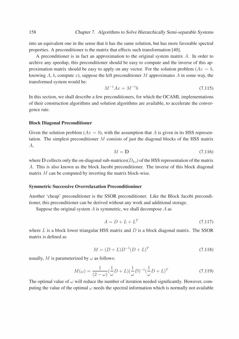
158 Chapter 7. Algorithms to Solve Hierarchically Semi-separable Systems
into an equivalent one in the sense that it has the same solution, but has more favorable spectral
properties. A preconditioner is the matrix that effects such transformation [40].
A preconditioner is in fact an approximation to the original system matrix A. In order to
archive any speedup, this preconditioner should be easy to compute and the inverse of this ap-
proximation matrix should be easy to apply on any vector. For the solution problem (Ax = b,
knowing A, b, compute x), suppose the left preconditioner M approximates A in some way, the
transformed system would be:
M−1Ax = M−1b (7.115)
In this section, we shall describe a few preconditioners, for which the OCAML implementations
of their construction algorithms and solution algorithms are available, to accelerate the conver-
gence rate.
Block Diagonal Preconditioner
Given the solution problem (Ax = b), with the assumption that A is given in its HSS represen-
tation. The simplest preconditioner M consists of just the diagonal blocks of the HSS matrix
A,
M = D (7.116)
whereD collects only the on-diagonal sub-matrices(Dk;i) of the HSS representation of the matrix
A. This is also known as the block Jacobi preconditioner. The inverse of this block diagonal
matrix M can be computed by inverting the matrix block-wise.
Symmetric Successive Overrelaxation Preconditioniner
Another ‘cheap’ preconditioner is the SSOR preconditioner. Like the Block Jacobi precondi-
tioner, this preconditioner can be derived without any work and additional storage.
Suppose the original system A is symmetric, we shall decompose A as
A = D + L + LT (7.117)
where L is a block lower triangular HSS matrix and D is a block diagonal matrix. The SSOR
matrix is defined as
M = (D + L)D−1(D + L)T (7.118)
usually, M is parameterized by ω as follows:
M(ω) =1
(2 − ω)(1
ωD + L)(
1
ωD)−1(
1
ωD + L)T (7.119)
The optimal value of ω will reduce the number of iteration needed significantly. However, com-
puting the value of the optimal ω needs the spectral information which is normally not available

7.9. Design of the HSS Iterative Solver 159
Figure 7.8: Fast model reduction on nodes. It reduces the HSS complexity of a node at the cost
of loss in data
in advance and prohibitively expensive to compute. The direct solution method of such block
triangular HSS system( 1ωD + L) has been presented in Section 7.5.
Fast Model Reduced Preconditioner
A downsweep model reduction can be done on the HSS representation to reduce its HSS com-
plexity at the cost of loss in data. Here, we only review the algorithm, for details on proof and
analysis, refer to [79].
Suppose A is a HSS matrix of which the HSS representation is defined by sequences U , V ,
R, W , B, D. The downsweep model reduction algorithm consists of two possible operations:
• Reduction at node/leaf: When needed, model reduction could be done on nodes. Given a
node like the one shown on the left of Figure 7.8, with the tolerance specified, we can de-
compose the translation matrices with economical rank revealing factorization as follows:
[Rk;2i−1 Bk;2i−1,2i
]= Uk;2i−1
[Rk;2i−1 Bk;2i−1,2i
]+ O(ǫ) (7.120)
[Rk;2i Bk;2i,2i−1
]= Uk;2i
[Rk;2i Bk;2i,2i−1
]+ O(ǫ) (7.121)
[W H
k;2i
Bk;2i,2i−1
]=
[W H
k;2i
Bk;2i−1,2i
]V H
k;2i + O(ǫ ′) (7.122)
[W H
k;2i−1
Bk;2i,2i−1
]=
[W H
k;2i−1
Bk;2i−1,2i
]V H
k;2i−1 + O(ǫ ′) (7.123)
Or equivalently: [Rk;2i−1 Bk;2i−1,2i
0 W Hk;2i
]

160 Chapter 7. Algorithms to Solve Hierarchically Semi-separable Systems
=
[Uk;2i−1 0
0 I
][Rk;2i−1 Bk;2i−1,2i
0 W Hk;2i
] [I 0
0 V Hk;2i
]+ O(ǫ ′) (7.124)
[Rk;2i Bk;2i,2i−1
0 W Hk;2i−1
]
=
[Uk;2i 0
0 I
][Rk;2i Bk;2i,2i−1
0 W Hk;2i−1
][I 0
0 V Hk;2i−1
]+ O(ǫ ′) (7.125)
Thus the translation matrices of this node have been reduced as: Rk;2i−1, Rk;2i, Wk;2i−1,
Wk;2i, Bk;2i−1,2i and Bk;2i,2i−1. The factors Uk;2i−1, Uk;2i, Vk;2i−1 and Vk;2i will be propa-
gated to its children and modified their translation matrices.
• Downsweep modification: after these factors Uk;i, Vk;i of a node are computed, they will
be swept to the children of this node, and modify their translation matrices as in Figure
7.8.
1. If the child is a non-leaf node
Rk;2i−1 = Rk;2i−1Uk;i, Rk;2i = Rk;2iUk;i (7.126)
Wk;2i−1 = Wk;2i−1Vk;i, Wk;2i = Wk;2iVk;i (7.127)
2. If the child is a leaf
Uk;i = Uk;iUk;i, V k;i = Vk;iVk;i (7.128)
After this modification, reduction method can be done on this modified node to reduce its
complexity. When the downsweep recursion reaches the leaves of the HSS representation,
the whole HSS representation has been model reduced under a certain tolerance.
Fast Model Reduction with HSS LU Factorization Preconditioner
It is known that the standard CGmethod only works for symmetric positive definite matrices. For
the matrices that are not symmetric positive definite, the standard CG method would converge
quite slowly or not at all. We will of course expect the transformed system to be symmetric
positive definite, if the original system is so.
The left preconditioner alone is often not what is used in practice; because the transformed
matrix M−1A is generally not symmetric, even though A and M are symmetric. Therefore, the
standard CG method is not immediately applicable to this system. We can of course use the CGS
and the BICG method which can handle nonsymmetric positive definite systems; however, it is
advantageous to use the standard CG method due to its simplicity and low computational cost in
each iteration.

7.9. Design of the HSS Iterative Solver 161
One way to remedy the preconditioner for the standard CG method is to LU factorize the left
preconditioner as M = M1M2, and apply M1 and M2 separately as the left preconditioner and
the right preconditioner. Then the original system would be transformed into the following:
M−11 AM−1
2 (M2x) = M−11 b (7.129)
Here M1 is called the left preconditioner; M2 is called the right precondtioner. If M is sym-
metric, that is M1 = MT2 (note that if the original HSS matrix is symmetric, the preconditioner
constructed by the algorithm presented in Section 7.9.1 is symmetric as well), one can easily
prove that the transformed coefficient matrix M−11 AM−1
2 is symmetric. Thus the standard CG
method is applicable again. M1 and M2 can be constructed by a LU factorization (details with
proof in Section. 7.3.5) on the HSS matrix M .
Summary on HSS Preconditioners
Summarizing Table 7.2 compares the preconditioners and their solution methods we proposed,
including effort and storage needed to construct these preconditioners.
Table 7.2: HSS preconditioners: construction and solution
Preconditioner Construction Storage
needed
Inverse solution Remarks
Block Jacobi without effort not
needed
direct inverse Only suitable for
diagonal dominant
matrix
Block SSOR without effort not
needed
HSS forward and
backward substitu-
tion [80]
simple double
sided precondi-
tioner
Fast model reduc-
tion
Model reduc-
tion [79]
needed Fast HSS di-
rect Solvers
[81, 82, 79, 83]
advanced, high
cost
Fast model reduc-
tion with LU fac-
torization
Model reduc-
tion and HSS
LU [80, 84]
needed HSS forward and
backward substitu-
tion [84, 80]
advanced double
sided precon-
ditioner, high
cost
7.9.2 Numerical Result
To study the behavior of the iterative HSS solver we developed, we choose to experiment with
the HSS CG, HSS CGS, HSS BiCG, HSS Bi-CGSTAB method and the direct HSS solver on

162 Chapter 7. Algorithms to Solve Hierarchically Semi-separable Systems
Figure 7.9: Numerical experiment with solvers: CPU time needed to solve system matrices of
different sizes with different solution methods
smooth matrices A defined as:
Aij =
c × n i = j
n|i−j| i/=j
(7.130)
(n is the dimension of the matrix, c is a parameter to control the diagonal dominance. We choose
the value of c to be 2, so that the matrix is positive definite.) The required solution accuracy
of iterative solver is specified to be 10−6; the initial guess for the solution is given as vector of
zeros; the right hand side is a random vector. The goal is to compute x so that Ax = b.
It can be seen that from Figure 7.9 that the CPU time needed by the HSS CG method is
comparable with that of the HSS direct solver. Among the CG like methods, the standard CG
method takes the least time, however, its applicability is not as good as that of the others. The
HSS CGS method takes about half of the time needed by the HSS BiCG method; however, it is
worth mentioning that the behavior of the CGS method is highly irregular. It may even fail to
deliver a solution when other CG variants do (the diverging cases are not plotted in Figure 7.9).
Bi-CGSTAB is more stable than CGS and it does not require the matrix transpose. These are
consistent with the analysis of these CG variants in [40]. It can also be seen from Figure 7.9 that
the time curve of iterative methods are irregular in general, while the direct solver scales well
with the size of the matrices (if the system matrices are smooth on off-diagonal sub-matrices).
One question still remains: under what situation should the iterative methods be preferred
over the direct solver? As we mentioned, the core operation of iterative methods is matrix-vector

7.9. Design of the HSS Iterative Solver 163
Figure 7.10: Numerical experiment with solvers on 2000× 2000 system matrices: the CPU time
needed to solve system matrices of fixed dimension with different smoothness
multiplication; this operation scales better with the HSS complexity than the direct HSS solution
method does. This indicates that the iterative methods should be adopted under the circumstance
that the off-diagonal sub-matrices of the HSS matrices is not of low rank. We conduct a series of
experiments to see how the iterative methods and direct method would scale with the smoothness.
We choose to work on the smooth matrix A defined as:
Aij =
c × n i = j
n × cos(k|i − j|π) i/=j(7.131)
Here, k is used to control the smoothness, a larger k would result in more high frequency com-
ponents, which would then result in less smooth matrices and increase the HSS complexity of
the HSS representation. n is the dimension of the matrix. n here is specified as 2000; that is the
matrices are of size 2000 × 2000. c controls diagonal dominance; we choose the value of c be
2. A series of experiments with different k is performed on the HSS CG method, the HSS direct
solution method and the direct solution method from LAPACK.
From Figure 7.10, we can see that the solution methods based on the HSS representation are
preferred when the system matrix is non-smooth; it is obvious that the direct solution method
does not scale well with the increasing value of k, while the CPU time needed by HSS CG
method increases smoothly with the value of k.
After the above comparison, it is safe to conclude that HSS iterative method should be pre-
164 Chapter 7. Algorithms to Solve Hierarchically Semi-separable Systems
ferred over direct HSS solution method, if the HSS complexity of the HSS representation is not
small compared to the dimension of the matrix. Or equivalently, the iterative method should be
preferred when the matrix is not very smooth. However if the matrix is completely not smooth,
the solution methods based on HSS representation described in this thesis are not recommended.
7.9.3 Conclusions on Iterative HSS Solvers
We studied the limitation of direct HSS solution method. A general strategy to combine the HSS
representation and its algorithms with iterative solution algorithms has been given. With this
strategy, any iterative algorithm can be easily combined with the HSS representations. We im-
plemented and tested a number of iterative solution algorithms based on HSS representations. All
these numerical experiments suggest that when the off-diagonal blocks of the system matrix are
not so smooth, the iterative algorithms based HSS representations exceed its direct counterpart in
CPU time and memory usage. We also proposed and implemented a number of preconditioners
based on HSS representation to improve the convergence of the iterative methods.
7.10 Final Remarks
Although the HSS theory is not yet developed to the same full extent as the sequentially semi-
separable theory, the results obtained so far show that the HSS structure has indeed a number of
very attractive properties that make it a welcome addition to the theory of structured matrices.
Fundamental operations such as matrix-vector multiplication, matrix-matrix multiplication and
matrix inversion (including theMoore-Penrose case accounted for in [76]) can all be excuted with
a computational complexity linear in the size of the matrix, and additional efficiency induced by
the translation operators. A representation in terms of global diagonal and shift operators is
also available, very much in the taste of the more restrictive multi-scale theory. These formulas
have not yet been exploited fully. The connection with time-varying system theory is also very
strong, and it should be possible in the future to transfer a number of its results to the HSS
representation, in particular model reduction, interpolation and Hankel norm approximation (i.e.
model reduction).

Chapter 8
3D Capacitance Extraction Based on Multi-Level
Hierarchical Schur Algorithm
Go down deep enough into anything and you will find
mathematics.
Dean Schlicter
In this chapter, we study the sparse inverse approximation algorithm used in SPACE, the
Layout-to-Circuit Extractor [2], and we apply some of the previously developed techniques for
efficient system inversion to the problem of 3D capacitance extraction. We also introduce a new
method based on Hierarchical Schur Interpolation. In Section 8.1, we briefly introduce SPACE
and discuss its limitations. Then, we propose some solutions to deal with these limitations and
present some numeric results. In Section 8.5, we combine the 2D Hierarchical Schur Algorithm
with Hierarchically semi-separable solver and demonstrate its accuracy and efficiency.
8.1 Introduction to SPACE
Parasitic capacitance of interconnects in integrated circuits has become more important as the
feature sizes on the circuits are decreased and the area of the circuit is unchanged or increased.
For sub-micron integrated circuits - where the vertical dimensions of the wires are in the same
order of magnitude as their minimum horizontal dimensions - 3D numerical techniques are even
required to accurately compute the values of the interconnect capacitances.
SPACE is a layout-to-circuit extraction program, that is used to accurately and efficiently
compute 3D interconnect capacitances of integrated circuits based upon their mask layout de-
scription. The 3D capacitances are part of an output circuit together with other circuit com-
ponents like transistors and resistances. This circuit can directly be used as input for a circuit
simulator like SPICE.
The boundary element method that is adopted in SPACE can be described briefly as follows:
1. For the purpose of modeling IC interconnections, it is sufficient to suppose that the chip is
stratified medium in which the conductors are floating. For such a medium, the potential
at a point p can be written as:
Φ(p) =
∫
D
G(p, q)ρ(q)dq, q ∈ D (8.1)
165

166 Chapter 8. 3D Capacitance Extraction Based on Multi-Level Hierarchical Schur Algorithm
where the Green’s function G(p, q) represents the potential induced at point p, due to a
unit point charge at point q. In this thesis, the Green’s function G(p, q) is computed with
the single integration formula presented in [85].
2. The above equations are transformed into a matrix equation by discretizing the surface
charge on the conductors as a piecewise linear and continuous distribution on a set of
boundary elements.
3. Let N be the total number of boundary elements, the matrix equation can be written as:
Φ = Gσ (8.2)
where Φ = [φ1, φ2...φN ]T and σ = [σ1, σ2...σN ]T collect the potentials of the boundary
elements and charges on the boundary elements respectively, and Gijσj is the potential
induced at the element i by the charge at the boundary element j.
4. Using this equation, we can compute the conductor capacitance as follows: let A be
an incidence matrix relating each boundary elements to the conductors, i.e. Aij = 1
if element i lies on conductor j, and Aij = 0 if otherwise. Also, let M be the total
number of conductors, V = [V1, V2, ..., VM ]T be the vector of conductor potentials and
Q = [Q1, Q2, ..., QM ]T be the vector charges on the conductors, then:
Q = ATG−1AV = CsV. (8.3)
Hence:
Cs = ATG−1A. (8.4)
5. The matrix Cs is the short circuit capacitance matrix. The capacitance network is derived
from the short circuit capacitance matrix as follows:
Cij = −Csij for i/=j, Cii =M∑
j=1
Csij. (8.5)
Consequently, the matrix G has to be generated and inverted. This matrix can be very big and
full. Generating and inverting such a matrix is prohibitively expensive. Moreover, the full matrix
would result in a too complicated circuit for sensible verification.
As a solution, SPACE adopts a scan-line algorithm, the generalized Schur algorithm and the
hierarchical Schur algorithm to compute a sparse inverse approximation of G−1, which is also
physically the low-complexity short circuit capacitance matrix. Thereby it ignores in effect small
capacitances between conductors that are physically “far” from each other. Let w be the param-
eter which denotes the distance over which capacitive coupling is significant. The CPU time
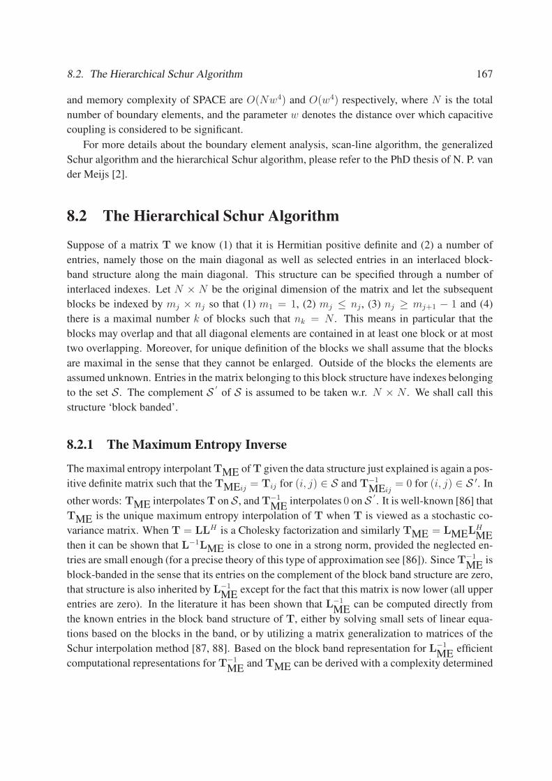
8.2. The Hierarchical Schur Algorithm 167
and memory complexity of SPACE are O(Nw4) and O(w4) respectively, where N is the total
number of boundary elements, and the parameter w denotes the distance over which capacitive
coupling is considered to be significant.
For more details about the boundary element analysis, scan-line algorithm, the generalized
Schur algorithm and the hierarchical Schur algorithm, please refer to the PhD thesis of N. P. van
der Meijs [2].
8.2 The Hierarchical Schur Algorithm
Suppose of a matrix T we know (1) that it is Hermitian positive definite and (2) a number of
entries, namely those on the main diagonal as well as selected entries in an interlaced block-
band structure along the main diagonal. This structure can be specified through a number of
interlaced indexes. Let N × N be the original dimension of the matrix and let the subsequent
blocks be indexed by mj × nj so that (1) m1 = 1, (2) mj ≤ nj, (3) nj ≥ mj+1 − 1 and (4)
there is a maximal number k of blocks such that nk = N . This means in particular that the
blocks may overlap and that all diagonal elements are contained in at least one block or at most
two overlapping. Moreover, for unique definition of the blocks we shall assume that the blocks
are maximal in the sense that they cannot be enlarged. Outside of the blocks the elements are
assumed unknown. Entries in the matrix belonging to this block structure have indexes belonging
to the set S. The complement S ′
of S is assumed to be taken w.r. N × N . We shall call this
structure ‘block banded’.
8.2.1 The Maximum Entropy Inverse
Themaximal entropy interpolantTME ofT given the data structure just explained is again a pos-
itive definite matrix such that the TMEij = Tij for (i, j) ∈ S and T−1
MEij= 0 for (i, j) ∈ S ′. In
other words: TME interpolatesT on S, andT−1
MEinterpolates 0 on S ′
. It is well-known [86] that
TME is the unique maximum entropy interpolation of T when T is viewed as a stochastic co-
variance matrix. When T = LLH is a Cholesky factorization and similarly TME = LMELHME
then it can be shown that L−1LME is close to one in a strong norm, provided the neglected en-
tries are small enough (for a precise theory of this type of approximation see [86]). SinceT−1
MEis
block-banded in the sense that its entries on the complement of the block band structure are zero,
that structure is also inherited by L−1
MEexcept for the fact that this matrix is now lower (all upper
entries are zero). In the literature it has been shown that L−1
MEcan be computed directly from
the known entries in the block band structure of T, either by solving small sets of linear equa-
tions based on the blocks in the band, or by utilizing a matrix generalization to matrices of the
Schur interpolation method [87, 88]. Based on the block band representation for L−1
MEefficient
computational representations for T−1
MEand TME can be derived with a complexity determined

168 Chapter 8. 3D Capacitance Extraction Based on Multi-Level Hierarchical Schur Algorithm
by the sizes of the blocks (not the size of the original matrix.) e.g. if T is tri-banded, then only
O(N) computations would be involved in computing all the results, thereby achieving optimal
computational complexity in that the number of computations is about equal to the number of
unknown data (also known as algebraic degrees of freedom).
8.2.2 One Level of Hierarchy Up: the ‘Nelis Method’
We now consider the case where we have, at the highest level of the hierarchy, a matrix consisting
of blocks, whereby the known elements in the individual blocks on the main diagonal and the
first side diagonals all have a block band structure as explained in the previous section (this
assumption can be generalized, but it is the most common one in practice so far).
To derive the gist of the hierarchical method, we specialize to the case where we have a n×n
block matrix. For ease of discussion we denote block decompositions of a matrix T with fat
script, hence
T =
T11 T12 T13 · · · T1n
T21 T22 T23 · · · ...
T31 T32 T33 · · · ...... · · · · · · . . .
...
Tn1 · · · · · · · · · Tnn
(8.6)
in which the known entries in TMEij = Tij are all block-banded matrices for |i − j| ≤ 1 and
the entries in |i − j| > 1 are totally unknown (remark the gaps with unknown entries between
the blocks). Again we assume T to be positive definite. From the theory of maximum entropy
interpolation [86], we know that there is a matrix TME which interpolates at the known entries
(in the known bands) and whose inverse interpolates zero in the complementary index set. That
is:
TME =
D1 AT2 ∗ · · · ∗
A2 D2 AT3 · · · ∗
∗ . . .. . .
. . . ATn
∗ ∗ ∗ An Dn
(8.7)
and
RME = T−1
ME=
R1 BT2 0 · · · 0
B2 R2 BT3 · · · 0
0. . .
. . .. . . BT
n
0 0 0 Bn Rn
(8.8)
where Di = Tii, Ai = Ti,i−1, ATi = Ti−1,i and ∗ are unknown block matrices. The problem
is that there is no known algorithm at present to compute the entries in the multi-block banded
inverse, as was the case for the Schur algorithm, except by optimizing on the maximum entropy
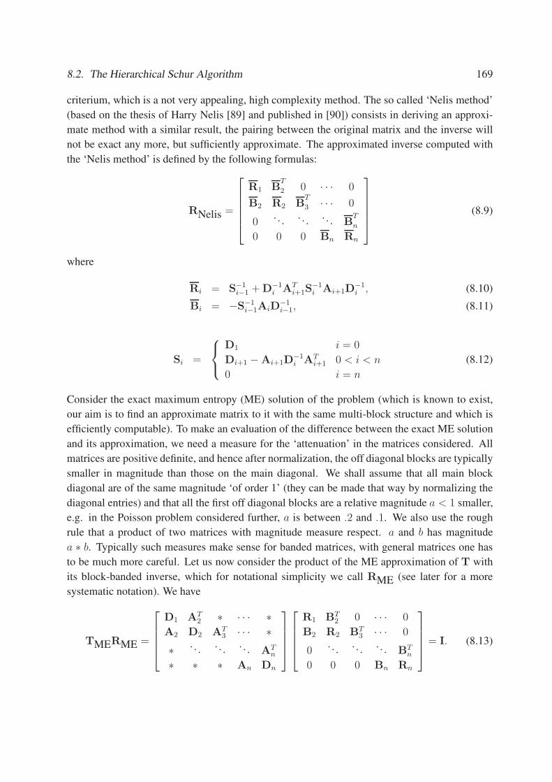
8.2. The Hierarchical Schur Algorithm 169
criterium, which is a not very appealing, high complexity method. The so called ‘Nelis method’
(based on the thesis of Harry Nelis [89] and published in [90]) consists in deriving an approxi-
mate method with a similar result, the pairing between the original matrix and the inverse will
not be exact any more, but sufficiently approximate. The approximated inverse computed with
the ‘Nelis method’ is defined by the following formulas:
RNelis =
R1 BT
2 0 · · · 0
B2 R2 BT
3 · · · 0
0. . .
. . .. . . B
T
n
0 0 0 Bn Rn
(8.9)
where
Ri = S−1i−1 + D−1
i ATi+1S
−1i Ai+1D
−1i , (8.10)
Bi = −S−1i−1AiD
−1i−1, (8.11)
Si =
D1 i = 0
Di+1 − Ai+1D−1i AT
i+1 0 < i < n
0 i = n
(8.12)
Consider the exact maximum entropy (ME) solution of the problem (which is known to exist,
our aim is to find an approximate matrix to it with the same multi-block structure and which is
efficiently computable). To make an evaluation of the difference between the exact ME solution
and its approximation, we need a measure for the ‘attenuation’ in the matrices considered. All
matrices are positive definite, and hence after normalization, the off diagonal blocks are typically
smaller in magnitude than those on the main diagonal. We shall assume that all main block
diagonal are of the same magnitude ‘of order 1’ (they can be made that way by normalizing the
diagonal entries) and that all the first off diagonal blocks are a relative magnitude a < 1 smaller,
e.g. in the Poisson problem considered further, a is between .2 and .1. We also use the rough
rule that a product of two matrices with magnitude measure respect. a and b has magnitude
a ∗ b. Typically such measures make sense for banded matrices, with general matrices one has
to be much more careful. Let us now consider the product of the ME approximation of T with
its block-banded inverse, which for notational simplicity we call RME (see later for a more
systematic notation). We have
TMERME =
D1 AT2 ∗ · · · ∗
A2 D2 AT3 · · · ∗
∗ . . .. . .
. . . ATn
∗ ∗ ∗ An Dn
R1 BT2 0 · · · 0
B2 R2 BT3 · · · 0
0. . .
. . .. . . BT
n
0 0 0 Bn Rn
= I. (8.13)

170 Chapter 8. 3D Capacitance Extraction Based on Multi-Level Hierarchical Schur Algorithm
In this equation, ∗ and their conjugates have no known entries, and we can find in the above equa-tion that: TME
31 = −A3B2R−11 , and hence it must be of relative magnitude a2. Subsequently,
with the assumption of decay a, we can prove that each off-diagonal matrices has additional a
decay. That is TMEij is of relative magnitude a|j−i| < 1.
We measure the difference between the ME approximation and the Nelis’s approximated
inverse by considering their product:
TMERNelis. (8.14)
By setting the error bound to be at leastO(a3), we may ignore allTMEij entries where |j−i| ≥ 3
and we have:
TMERNelis =
D1 AT2 TME
13 · · · 0
A2 D2 AT3 · · · 0
0. . .
. . .. . . AT
n
0 0 TMEn,n−2 An Dn
RNelis + O(a3) (8.15)
and ignoring the O(a3) entries in the product, we have:
TMERNelis =
I C2 0 · · · 0
E2 I C3 · · · 0
0. . .
. . .. . . Cn
0 0 0 En I
+ O(a3) (8.16)
where
Ei = Ai(S−1i−2 −D−1
i−1), (8.17)
Ci = ATi D−1
i ATi+1S
−1i Ai+1D
−1i . (8.18)
All Ei and Ci terms are of at leastO(a3), either from the original assumption or by construction.
For most entries this is clear, remark that:
Si =
D1 i = 0
Di+1 − Ai+1D−1i AT
i+1 0 < i < n
0 i = n
(8.19)
such that: Si = Di+1 + O(a2). Therefore:
TMERNelis = I + O(a3). (8.20)
Hence, we say:
Theorem 8.1. the Nelis’ approximated inverse RNelis is a O(a3) order approximation to the
Maximum Entropy inverse RME.

8.3. Limitations of the Algorithms Used in SPACE 171
8.3 Limitations of the Algorithms Used in SPACE
Although, SPACE is very efficient in generating the capacitance network for 3D layouts, we
believe the underlying algorithms do have some limitations and we can improve them easily.
1. Although SPACE extracts capacitance networks for three dimensional layouts, we may
describe its algorithm as 2.5D in the sense that it assumes the vertical dimension of the
layouts to be very thin. This assumption was quite valid at the time when SPACE came
out [2]. However, after many years of development in VLSI technology, circuits with many
more layers are common and the vertical dimension can not be ignored anymore. In fact,
if we assume the vertical dimension to be comparable with the horizontal dimensions, the
CPU time complexity of SPACE quickly becomes O(N5/3w4) which is not linear in the
total number of panels.
2. Again, when the vertical dimension can not be ignored, the memory complexity of SPACE
becomes O(N2/3w4), which not only means that much more memory is needed, but also
indicates that much more entities in the Green’s function matrix must be computed. The
computation of Green’s functions is a major factor of the CPU time needed.
3. Due to historical reasons, SPACE adopts the Hierarchical Schur algorithm in the X axis
and then apply the Schur algorithm on the Y axis. This is not a very consistent scheme, in
the sense that, with this kind of scheme, SPACE with exactly the same configuration would
generate different capacitance network for the same layout depending on which direction
the layout aligns with.
Out of the considerations above, we propose a multi-level hierarchical Schur algorithm which
we shall present in the following sections.
8.4 Multi-Level Hierarchical Schur Algorithm
The straight-forward idea is to apply the hierarchical Schur algorithm along both the X and Y
axes. We can even go further by applying the hierarchical Schur algorithm along X, Y and Z axes.
In this way, we can efficiently deal with a genuine three dimensional layout. In this section, we
refer to these algorithms as multi-level hierarchical Schur algorithms.
8.4.1 Notations
Before we present the Multi-level hierarchical Schur algorithms, we would like to introduce a
few notations that will be used consistently hereafter in this chapter.

172 Chapter 8. 3D Capacitance Extraction Based on Multi-Level Hierarchical Schur Algorithm
• Let the 3D layout of interconnects be discretized with boundary elements; Lx, Ly, Lz be
its maximum dimensions in x, y, z axes, respectively.
• Let x0, y0, z0 be the smallest coordinates of the layout in x, y and z axes, we have the layout
completely embedded in the bounding box Ω; x0 ≤ x ≤ x0 +Lx, y0 ≤ y ≤ y0 +Ly, z0 ≤z ≤ z0 + Lz.
• Assume a certain 2D scan-window of dimensionswx×wy, Ω(i, j); 1 ≤ i ≤ ⌈Lx/wx⌉, 1 ≤i ≤ ⌈Ly/wy⌉ denotes a sub-domain that x0 +(i−1)×wx ≤ x ≤ x0 + i×wx, y0 +(j−1)×wy ≤ y ≤ y0 + j ×wy, z0 ≤ z ≤ z0 + Lz which is bounded in the 2D scan-window
W(i, j).
• Assume a certain 3D scan-window of dimensions wx × wy × wz, Ω(i, j, k); 1 ≤ i ≤⌈Lx/wx⌉, 1 ≤ i ≤ ⌈Ly/wy⌉, 1 ≤ i ≤ ⌈Lz/wz⌉ denotes a sub-domain x0+(i−1)×wx ≤x ≤ x0 + i×wx, y0+(j−1)×wy ≤ y ≤ y0+j×wy , z0+(k−1)×wz ≤ z ≤ z0 + i×wzwhich is bounded in the 3D scan-windowW(i, j, k).
• Let ∪ be a binary merging operator that collects boundary elements from both sub-domains
and number them locally, for instance, Ω(i, j)∪Ω(i, j + 1) or equivalently⋃j+1
m=j Ω(i, m).
• Let G be an operator which generates a matrix of Green’s functions for all boundary el-
ements in a certain domain/sub-domain, for instance, G(Ω(i, j, k)) produces the matrix
GΩ(i,j,k) which contains all Green’s functions for the boundary elements within the sub-
domain Ω(i, j, k). For this matrix, a local numbering of the boundary elements is used.
• Let [GΩ(i,j,k)
]or equivalently [G(Ω(i, j, k))] denote an embedding process that takes
the matrix GΩ(i,j,k) with local numbering and embeds it into a larger empty matrix (ma-
trix with only zero entries) according to the map between the local numbering and global
numbering of the boundary elements. The embedding operator can be specified more pre-
cisely. Assume there are M boundary elements that are locally numbered in Ω(i, j, k), and
there are N boundary elements that are globally numbered in Ω. Then there is a unique
incidence matrix IΩ(i,j,k) of dimension M × N that maps the local indexes to the global
indexes, i.e IΩ(i,j,k)(m, n) = 1 if the boundary with local index m is numbered with global
index n. IΩ(i,j,k)(m, n) = 0, if otherwise. The transpose of this incidence matrix maps the
global indexes to the local indexes. We have:
[GΩ(i,j,k)
]= IΩ(i,j,k)GΩ(i,j,k)I
TΩ(i,j,k). (8.21)
Apparently, the incidence matrix has the following property:
ITΩ(i,j,k)IΩ(i,j,k) = I. (8.22)
Here, I denotes a identity matrix of dimensions M × M .
• G−1
SIdenotes a sparse approximation of G−1.

8.4. Multi-Level Hierarchical Schur Algorithm 173
8.4.2 Two Dimensional Scan-window Algorithm
With the whole layout discretized with boundary elements and then segmented with 2D scan-
windows of size w × w, the sparse inverse to the G is defined as:
G−1
SI=
⌈Lx/w⌉−1∑
i=1
⌈Ly/w⌉−1∑
j=1
[G−1(
i+1⋃
m=i
j+1⋃
n=j
Ω(m, n))] −⌈Ly/w⌉−1∑
j=2
[G−1(
i+1⋃
m=i
Ω(m, j))]
−⌈Lx/w⌉−1∑
i=2
⌈Ly/w⌉−1∑
j=1
[G−1(
j+1⋃
n=j
Ω(i, n))] −⌈Ly/w⌉−1∑
j=2
[G−1(Ω(i, j))]. (8.23)
Next we may replace the G−1 in Eq. (8.4) with the above sparse approximation and we have:
Cs ≈ AT
⌈Lx/w⌉−1∑
i=1
⌈Ly/w⌉−1∑
j=1
[G−1(
i+1⋃
m=i
j+1⋃
n=j
Ω(m, n))] −⌈Ly/w⌉−1∑
j=2
[G−1(
i+1⋃
m=i
Ω(m, j))]
−⌈Lx/w⌉−1∑
i=2
⌈Ly/w⌉−1∑
j=1
[G−1(
j+1⋃
n=j
Ω(i, n))] −⌈Ly/w⌉−1∑
j=2
[G−1(Ω(i, j))]A. (8.24)
Let Cs(Ω(i, j)) = AT[G−1(Ω(i, j))]A denote the (partial) short-circuit capacitance matrix
generated for Ω(i, j). With the definition of the embedding operator, We can write
Cs(Ω(i, j)) = AT IΩ(i,j)G−1(Ω(i, j))IT
Ω(i,j)A. (8.25)
We also have a local incidence matrix AΩ(i,j) that relates boundary elements with local indexes
to conductor potential, i.e AΩ(i,j)(m, n) = 1 if the boundary element with the local index m lies
on the conductor n, and 0 if otherwise. Due to the fact that Eq. (8.25) only involves the boundary
elements in Ω(i, j), the additional information in A that counts other boundary elements will not
be taken into account. We have:
Cs(Ω(i, j)) = AT IΩ(i,j,k)G−1(Ω(i, j))IT
Ω(i,j,k)A
= ATΩ(i,j)I
TΩ(i,j)IΩ(i,j)G
−1(Ω(i, j))ITΩ(i,j)IΩ(i,j)AΩ(i,j)
= ATΩ(i,j)G
−1(Ω(i, j))AΩ(i,j). (8.26)
We may compute the global approximated short-circuit capacitance matrix as:
Cs ≈⌈Lx/w⌉−1∑
i=1
⌈Ly/w⌉−1∑
j=1
Cs(
i+1⋃
m=i
j+1⋃
n=j
Ω(m, n)) −⌈Ly/w⌉−1∑
j=2
Cs(
i+1⋃
m=i
Ω(m, j))
−⌈Lx/w⌉−1∑
i=2
⌈Ly/w⌉−1∑
j=1
Cs(
j+1⋃
n=j
Ω(i, n)) −⌈Ly/w⌉−1∑
j=2
Cs(Ω(i, j)). (8.27)

174 Chapter 8. 3D Capacitance Extraction Based on Multi-Level Hierarchical Schur Algorithm
Explicit computation of the matrix inverse is not recommended. Therefore, we may compute
G−1(Ω(i, j))AΩ(i,j) by solving a system of linear equations, G(Ω(i, j))x = AΩ(i,j) . Both a
direct solution method and an iterative solution method can be used here.
Note that global indexes and global incidence matrices do not appear in the above formula
and we do not have to compute them explicitly. All computations can remain local. As soon
as a (partial) short-circuit capacitance matrix is generated, we will use it to modify the short-
circuit capacitance matrix of the whole layout. Therefore, the program only has to analyse a
(small) segment of the whole circuit at any instant. This enables the algorithm to deal with large
circuits while consuming little computer memory. For more details, we refer to the PhD thesis of
Dr. N. P. van der Meijs [2] and we invite interested readers to look into prototype that we have
implemented.
Analysis of Computational Complexity
Let the lengths in the three axes be comparable, the total number of two dimensional scan-
windows is of O(N2/3w−2). The total number of panels inside each scan-window is of order
O(N1/3w2). A system of linear equations is to be solved in each scan-window and the complexity
is of O(w6N). Therefore, assuming the lengths in the three axes be comparable, the CPU time
complexity of this algorithm is of O(N5/3w4). Its memory complexity is of O(N2/3w4).
8.4.3 Three Dimensional Scan-window Algorithm
Similarly, we may apply the scan-window algorithm along X, Y and Z axes. We assume that the
whole layout is discretized with boundary elements and then segmented with 3D scan-windows
of size w × w × w. The sparse inverse to G is then defined as:
G−1
SI=
⌈Lx/w⌉−1∑
i=1
⌈Ly/w⌉−1∑
j=1
⌈Lz/w⌉−1∑
k=1
[G−1(Ω1)] −⌈Lz/w⌉−1∑
k=2
[G−1(Ω2)]
−⌈Ly/w⌉−1∑
j=2
⌈Lz/w⌉−1∑
k=1
[G−1(Ω3)] −⌈Lz/w⌉−1∑
k=2
[G−1(Ω4)]
−⌈Lx/w⌉−1∑
i=2
⌈Ly/w⌉−1∑
j=1
⌈Lz/w⌉−1∑
k=1
[G−1(Ω5)] −⌈Lz/w⌉−1∑
k=2
[G−1(Ω6)]
−⌈Ly/w⌉−1∑
j=2
⌈Lz/w⌉−1∑
k=1
[G−1(Ω7)] −⌈Lz/w⌉−1∑
k=2
[G−1(Ω8)] (8.28)
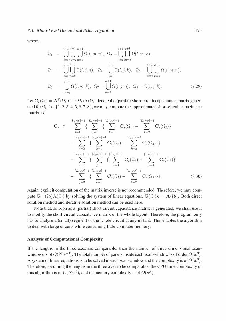
8.4. Multi-Level Hierarchical Schur Algorithm 175
where:
Ω1 =i+1⋃
l=i
j+1⋃
m=j
k+1⋃
n=k
Ω(l, m, n), Ω2 =i+1⋃
l=i
j+1⋃
m=j
Ω(l, m, k),
Ω3 =
i+1⋃
l=i
k+1⋃
n=k
Ω(l, j, n), Ω4 =
i+1⋃
l=i
Ω(l, j, k), Ω5 =
j+1⋃
m=j
k+1⋃
n=k
Ω(i, m, n),
Ω6 =
j+1⋃
m=j
Ω(i, m, k), Ω7 =
k+1⋃
n=k
Ω(i, j, n), Ω8 = Ω(i, j, k). (8.29)
Let Cs(Ωl) = AT (Ωl)G−1(Ωl)A(Ωl) denote the (partial) short-circuit capacitance matrix gener-
ated forΩl; l ∈ 1, 2, 3, 4, 5, 6, 7, 8, we may compute the approximated short-circuit capacitance
matrix as:
Cs ≈⌈Lx/w⌉−1∑
i=1
⌈Ly/w⌉−1∑
j=1
⌈Lz/w⌉−1∑
k=1
Cs(Ω1) −⌈Lz/w⌉−1∑
k=2
Cs(Ω2)
−⌈Ly/w⌉−1∑
j=2
⌈Lz/w⌉−1∑
k=1
Cs(Ω3) −⌈Lz/w⌉−1∑
k=2
Cs(Ω4)
−⌈Lx/w⌉−1∑
i=2
⌈Ly/w⌉−1∑
j=1
⌈Lz/w⌉−1∑
k=1
Cs(Ω5) −⌈Lz/w⌉−1∑
k=2
Cs(Ω6)
−⌈Ly/w⌉−1∑
j=2
⌈Lz/w⌉−1∑
k=1
Cs(Ω7) −⌈Lz/w⌉−1∑
k=2
Cs(Ω8). (8.30)
Again, explicit computation of the matrix inverse is not recommended. Therefore, we may com-
pute G−1(Ωl)A(Ωl) by solving the system of linear equations, G(Ωl)x = A(Ωl). Both direct
solution method and iterative solution method can be used here.
Note that, as soon as a (partial) short-circuit capacitance matrix is generated, we shall use it
to modify the short-circuit capacitance matrix of the whole layout. Therefore, the program only
has to analyse a (small) segment of the whole circuit at any instant. This enables the algorithm
to deal with large circuits while consuming little computer memory.
Analysis of Computational Complexity
If the lengths in the three axes are comparable, then the number of three dimensional scan-
windows is ofO(Nw−3). The total number of panels inside each scan-window is of orderO(w3).
A system of linear equations is to be solved in each scan-window and the complexity is ofO(w9).
Therefore, assuming the lengths in the three axes to be comparable, the CPU time complexity of
this algorithm is of O(Nw6), and its memory complexity is of O(w6).
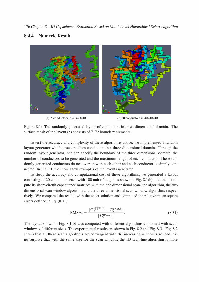
176 Chapter 8. 3D Capacitance Extraction Based on Multi-Level Hierarchical Schur Algorithm
8.4.4 Numeric Result
(a)15 conductors in 40x40x40 (b)20 conductors in 40x40x40
Figure 8.1: The randomly generated layout of conductors in three dimensional domain. The
surface mesh of the layout (b) consists of 7172 boundary elements.
To test the accuracy and complexity of these algorithms above, we implemented a random
layout generator which grows random conductors in a three dimensional domain. Through the
random layout generator, one can specify the boundary of the three dimensional domain, the
number of conductors to be generated and the maximum length of each conductor. These ran-
domly generated conductors do not overlap with each other and each conductor is simply con-
nected. In Fig 8.1, we show a few examples of the layouts generated.
To study the accuracy and computational cost of these algorithms, we generated a layout
consisting of 20 conductors each with 100 unit of length as shown in Fig. 8.1(b), and then com-
pute its short-circuit capacitance matrices with the one dimensional scan-line algorithm, the two
dimensional scan-window algorithm and the three dimensional scan-window algorithm, respec-
tively. We compared the results with the exact solution and computed the relative mean square
errors defined in Eq. (8.31).
RMSEc =‖Capprox
s −Cexacts ‖
‖Cexacts ‖ . (8.31)
The layout shown in Fig. 8.1(b) was computed with different algorithms combined with scan-
windows of different sizes. The experimental results are shown in Fig. 8.2 and Fig. 8.3. Fig. 8.2
shows that all these scan algorithms are convergent with the increasing window size, and it is
no surprise that with the same size for the scan window, the 1D scan-line algorithm is more

8.4. Multi-Level Hierarchical Schur Algorithm 177
0.4 0.5 0.6 0.7 0.8 0.9 1 1.1 1.2 1.3−3.5
−3
−2.5
−2
−1.5
−1
The length of scan−window (base 10 logarithmic axis)
RM
SE
(b
ase
10
lo
ga
rith
mic
ax
is)
RMSE vs the length of scan−window
1D scan−line
2D scan−window
3D scan−window
3D adaptive scan−window
Figure 8.2: The relative mean square errors in the computed short-circuit capacitance matrices.
0.4 0.5 0.6 0.7 0.8 0.9 1 1.1 1.2 1.3
2.6
2.8
3
3.2
3.4
3.6
3.8
4
4.2
4.4
The length of scan−window (base 10 logarithmic axis)
CP
U t
ime
(s)
bas
e 10 l
ogar
ithm
ic a
xis
CPU time vs the length of scan−window
1D scan−line
2D scan−window
3D scan−window
3D adaptive scan−window
Figure 8.3: The CPU time needed to computed the short-circuit capacitance matrices Vs the
scan-window size.

178 Chapter 8. 3D Capacitance Extraction Based on Multi-Level Hierarchical Schur Algorithm
accurate than the 2D scan-window algorithm, which is slightly more accurate than the 3D scan-
window algorithm. It is also clear that the total RMSE error is dominated by the approximation
made at the higher levels. Fig. 8.2 shows that the 3D scan-window algorithm is more efficient
than the other two algorithms. It also confirms that the CPU time needed for the 3D scan-
window algorithm increases more sharply with the size of the scan-window. Other than these,
we also observed that all three algorithms deliver more accurate result when more conductors
are clustered together. This is because nearby conductors shield each other and local interactions
become more dominate.
8.4.5 Adaptive Three Dimensional Scan-window Algorithm
As shown in Fig. 8.2, the error made by scanning along the X axis dominates the total relative
mean square error. A larger scan window along Y and Z axes would not help too much as
long as the scan-window along X axis is small. Therefore, it is reasonable to use a bigger scan
window along the X axis and decrease the size of scan-window along Y axis and Z axis. That
is wx > wy > wz > 0. Assuming that the whole layout is discretized with boundary elements
and then segmented with 3D scan-windows of size wx ×wy ×wz, the sparse inverse to G is then
defined as:
G−1
SI=
⌈Lx/wx⌉−1∑
i=1
⌈Ly/wy⌉−1∑
j=1
⌈Lz/wz⌉−1∑
k=1
[G−1(Ω1)] −⌈Lz/wz⌉−1∑
k=2
[G−1(Ω2)]
−⌈Ly/wy⌉−1∑
j=2
⌈Lz/wz⌉−1∑
k=1
[G−1(Ω3)] −⌈Lz/wz⌉−1∑
k=2
[G−1(Ω4)]
−⌈Lx/wx⌉−1∑
i=2
⌈Ly/wy⌉−1∑
j=1
⌈Lz/wz⌉−1∑
k=1
[G−1(Ω5)] −⌈Lz/wz⌉−1∑
k=2
[G−1(Ω6)]
−⌈Ly/wy⌉−1∑
j=2
⌈Lz/wz⌉−1∑
k=1
[G−1(Ω7)] −⌈Lz/wz⌉−1∑
k=2
[G−1(Ω8)] (8.32)
where Ωl; l ∈ 1, 2, 3, 4, 5, 6, 7, 8 is defined in Eq. (8.29). LetCs(Ωl) = AT (Ωl)G−1(Ωl)A(Ωl)
denote the (partial) short-circuit capacitance matrix generated for Ωl; l ∈ 1, 2, 3, 4, 5, 6, 7, 8,

8.5. Multi-Level Hierarchical Schur Algorithm Combined with HSS Solver 179
we may compute the approximated short-circuit capacitance matrix as:
Cs ≈⌈Lx/wx⌉−1∑
i=1
⌈Ly/wy⌉−1∑
j=1
⌈Lz/wz⌉−1∑
k=1
Cs(Ω1) −⌈Lz/wz⌉−1∑
k=2
Cs(Ω2)
−⌈Ly/wy⌉−1∑
j=2
⌈Lz/wz⌉−1∑
k=1
Cs(Ω3) −⌈Lz/wz⌉−1∑
k=2
Cs(Ω4)
−⌈Lx/wx⌉−1∑
i=2
⌈Ly/wy⌉−1∑
j=1
⌈Lz/wz⌉−1∑
k=1
Cs(Ω5) −⌈Lz/wz⌉−1∑
k=2
Cs(Ω6)
−⌈Ly/wy⌉−1∑
j=2
⌈Lz/wz⌉−1∑
k=1
Cs(Ω7) −⌈Lz/wz⌉−1∑
k=2
Cs(Ω8). (8.33)
To study the accuracy and computational cost of the adaptive 3D scan-window algorithm, we
compute the short-circuit capacitance matrices of the layout as shown in Fig. 8.1(b). Then we
compare the result with the exact solution. The relative mean square error is defined in Eq. (8.31).
As shown in Fig. 8.2 and Fig. 8.3, the adaptive 3D scan-window algorithm achieves compa-
rable accuracy with much less computational time. Note that one can apply different schemes to
decrease the size of scan-windows, and they may deliver different results.
8.5 Multi-Level Hierarchical Schur Algorithm Combined with
HSS Solver
Other than the (adaptive) three dimensional scan-window algorithm, we can also compute a
three dimensional layout with the two dimensional scan-window algorithm combined with the
Hierarchically Semi-Separable solver.
8.5.1 Fast Hierarchically Semi-Separable Solver
In Chapter 7, we have presented the concept of the Hierarchically Semi-separable Systems and
its algorithms in full detail. As shown in the numeric experiments of Sec. 7.9.2, a matrix with
smooth kernel has a very efficient Hierarchically Semi-separable representation, and all matrix
operations on its HSS representation can be done with linear computational complexity, appar-
ently, the solution of a matrix-vector equation is one of these algorithms. A description of these
fast HSS solution algorithms can be found in [38] and [73]. In Sec. 7.9.2, we have studied
and demonstrated the efficiency of the fast HSS solution algorithm. In addition to that, a fast
and stable HSS representation construction algorithm of computation complexity O(N2) can
be found in [91]. However, without complicated reordering scheme such as nested-dissection

180 Chapter 8. 3D Capacitance Extraction Based on Multi-Level Hierarchical Schur Algorithm
[92, 93, 94], the system matrix generated with BEM for 2D or 3D layouts is not hierarchically
semi-separable. That is why we need to apply the two dimensional scan-window algorithm pre-
sented in Sec. 8.4.2, and within each scan-window, we only need to solve an one-dimensional
system of linear equations G(Ω(i, j))x = AΩ(i,j). With appropriate numbering for boundary
elements, G(Ω(i, j)) has only low rank off-diagonal sub-matrices. Therefore we can represent
with a very efficient HSS representation.
Numeric Experiments on HSS Representation Construction and Solution
Let N be the dimension of the system matrix, the HSS representation construction and solu-
tion algorithm together are of computational complexity O(N2). A direct solution method is
of computational complexity O(N3). Various factorization operations on small matrices are
needed for the HSS algorithms, therefore, the HSS construction and solution algorithms should
have a bigger overhead compared to the direct solution method. So, we predict that the HSS
construction&solution algorithms should be slower than the direct solution method for small
matrices but perform better when the matrices exceed certain threshold in dimension. We need
to find this threshold to obtain overall good performance. Unfortunately, it appears to be highly
implementation-depended. We can get an idea of this with some numeric experiments. Let A be
a smooth matrix of dimensions n × n, defined as:
Aij =
1 i = j1
|i−j|i/=j
(8.34)
Although it is not exactly the one dimensional Green’s function matrix, it resembles the one
dimensional Green’s function matrix quite well (as it has a “1/r” decay) and should have similar
properties. In fact, the matrix A is almost the same matrix as the one dimensional Green’s
function matrix where uniform discretization is used. We generate some random vector for
the right hand side b. We shall solve the system of linear equations Ax = b with both HSS
construction&solution algorithm and direct solution method (LAPACK routine). As we increase
n, we have tried to find out at what point the HSS algorithms will perform better. Concerning
the parameters for the HSS construction algorithm, the maximum dimension km of each Dn;i
matrix is 40 and the truncation tolerance tsvd for each economic SVD factorization is 10−3. As
shown in Fig. 8.4, the break even point is n = 700, after which the HSS construction&solution
algorithm is faster and the CPU time needed for direct solution method increases with n much
faster than the former. As shown in Fig. 8.5, although economic SVD factorizations are used to
construct HSS representations and for each economic SVD factorization, singular values that are
less than 10−3 are ignored, the HSS construction&solution method delivers accurate solutions.
To obtain even more accurate result, we only have to make the truncation tolerance tsvd smaller.
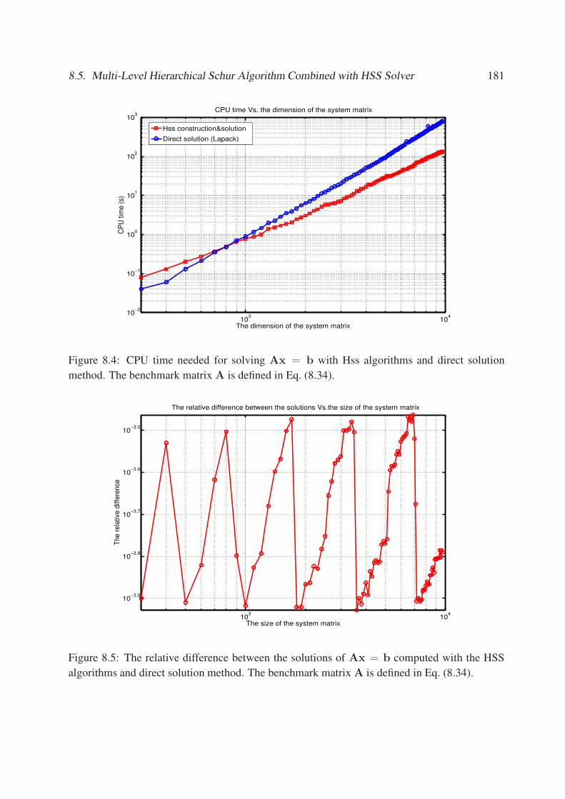
8.5. Multi-Level Hierarchical Schur Algorithm Combined with HSS Solver 181
103
104
10−2
10−1
100
101
102
103
CPU time Vs. the dimension of the system matrix
The dimension of the system matrix
CP
U tim
e (
s)
Hss construction&solution
Direct solution (Lapack)
Figure 8.4: CPU time needed for solving Ax = b with Hss algorithms and direct solution
method. The benchmark matrix A is defined in Eq. (8.34).
103
104
10−3.9
10−3.8
10−3.7
10−3.6
10−3.5
The size of the system matrix
The r
ela
tive d
iffere
nce
The relative difference between the solutions Vs.the size of the system matrix
Figure 8.5: The relative difference between the solutions of Ax = b computed with the HSS
algorithms and direct solution method. The benchmark matrix A is defined in Eq. (8.34).
182 Chapter 8. 3D Capacitance Extraction Based on Multi-Level Hierarchical Schur Algorithm
8.5.2 The HSS Assisted 2D Scan-window Algorithm
The HSS assisted algorithm is quite similar to the 2D scan-windows algorithm presented in
Section 8.4.2. With the whole layout be discretized with boundary elements and then segmented
with 2D scan-windows of size w × w, the sparse inverse to the G is defined as:
G−1
SI=
⌈Lx/w⌉−1∑
i=1
⌈Ly/w⌉−1∑
j=1
[G−1(
i+1⋃
m=i
j+1⋃
n=j
Ω(m, n))] −⌈Ly/w⌉−1∑
j=2
[G−1(
i+1⋃
m=i
Ω(m, j))]
−⌈Lx/w⌉−1∑
i=2
⌈Ly/w⌉−1∑
j=1
[G−1(
j+1⋃
n=j
Ω(i, n))] −⌈Ly/w⌉−1∑
j=2
[G−1(Ω(i, j))]. (8.35)
Let Cs(Ω(i, j)) = ATΩ(i,j)G
−1(Ω(i, j))AΩ(i,j), we may compute the global approximated short-
circuit capacitance matrix as:
Cs ≈⌈Lx/w⌉−1∑
i=1
⌈Ly/w⌉−1∑
j=1
Cs(i+1⋃
m=i
j+1⋃
n=j
Ω(m, n)) −⌈Ly/w⌉−1∑
j=2
Cs(i+1⋃
m=i
Ω(m, j))
−⌈Lx/w⌉−1∑
i=2
⌈Ly/w⌉−1∑
j=1
Cs(
j+1⋃
n=j
Ω(i, n)) −⌈Ly/w⌉−1∑
j=2
Cs(Ω(i, j)). (8.36)
To compute G−1(Ω(i, j))AΩ(i,j) or rather, to solve x in G(Ω(i, j))x = AΩ(i,j), we use the
direct elimination method (Lapack routine) to solve the system of linear equations, when the
dimension of G(Ω(i, j)) is smaller than certain threshold (which is experimentally determined
as 800). Otherwise, we first construct a HSS representation for G(Ω(i, j)) with the fast and
stable HSS construction algorithm [91], then solve G(Ω(i, j))x = AΩ(i,j) for x with the fast
HSS solution method. Let M be the total number of boundary elements in the scan-window, the
construction algorithm is of O(M2) computational complexity and the HSS solution algorithm
is of O(M) computational complexity. Very similar to the plain 2D scan-window algorithm
presented in Section 8.4.2, global indexes and global incidence matrices do not appear in the
formula and we do not have to compute them explicitly. All computations can remain local. As
soon as a (partial) short-circuit capacitance matrix is generated, we use it to modify the short-
circuit capacitance matrix of the whole layout.
Numeric Result
To study the efficiency of the HSS assisted 2D scan-window algorithm, we randomly generated
a complex interconnect layout which consisted of 100 conductors each with around 100 units
of length as shown in Fig. 8.6. The whole structure is bounded in a 40 × 40 × 40 box. The
structure is deep in the Z direction, therefore the layout can not be treated as 2.5D structure.
We computed the short capacitance matrix of this layout with 2D scan-window algorithm, HSS

8.5. Multi-Level Hierarchical Schur Algorithm Combined with HSS Solver 183
Figure 8.6: A randomly generated interconnect layout which consists of 100 conductors each
with around 100 units of length. The whole structure is bounded in a 40 × 40 × 40 box.
Table 8.1: CPU time needed for computing the layout shown in Fig. 8.6
2D scan-window HSS + 2D scan-window 3D scan-window
1.762178e+04 (s) 1.765510e+04 (s) 8.422940e+03 (s)
assisted 2D scan-window algorithm and 3D scan-window algorithm with the scan-window of
4 units in dimension. The whole structure has 24884 boundary elements. Hence we could not
afford to compute the exact short capacitance matrix, neither could we compare the accuracy of
these algorithms with respect to the exact solution. However, with the numeric experiments we
presented in Section 8.4.4, we may assume with confidence that the approximated solutions are
convergent to the exact solution.
Furthermore, since the HSS solution method is almost as accurate as the direct solution
method (as shown in Fig. 8.5), we may assume that the accuracy of the HSS assisted 2D scan-
window algorithm is close to that of the 2D scan-window algorithm and better than that of the
3D scan-window algorithm. As shown in Tab. 8.1, the computational time needed for the HSS
assisted 2D scan-window algorithm is slightly more than that needed for the 2D scan-window al-
gorithm but much higher that needed for the 3D scan-window algorithm. A careful study shows
that a large amount of the CPU time is spent on building the HSS representation. Therefore,
a straight-forward application of the HSS construction&solution algorithm does not help to re-
duce the total computational cost, neither would it deliver a more accurate solution. To make
this algorithm useful, we need to explore the regularity of the layout structure and recycle the

184 Chapter 8. 3D Capacitance Extraction Based on Multi-Level Hierarchical Schur Algorithm
precomputed HSS representation as we shall present in Section 8.5.3.
8.5.3 Reusing the HSS Representation
To be able to reuse an existing HSS representation, we have to make the following assumptions:
1. The conductor layout Ω is fairly regular. For instance, the layout can be specified with a
number of 3D boxes.
2. There is a fully connected mesh ΩF , such that every boundary element in each 2D scan-
windowΩ(m, n) can be found in the fully connected mesh. That is, the boundary elements
in Ω(m, n) is a sub-set of the boundary elements in ΩF .
Let GΩFbe the Green’s function matrix generated for ΩF , then we can generate every local
Green’s functions matrix by eliminating some rows and columns of GΩF, as we demonstrate in
Fig. 8.7. Similarly, once we have the HSS representation of GΩFat our disposal, we can con-
struct the HSS representation of the local Green’s functions matrices by eliminating the column
bases and row bases of the HSS representation of GΩF. These operations are of linear compu-
tational complexity. Therefore, the CPU time spent on constructing HSS representations will
be significantly reduced. With the HSS representation of the local Green’s functions matrices
constructed, the system of linear equations can also be solved efficiently.
8.5.4 Analysis of Computational Complexity
Let the lengths in the three axes be comparable, the number of two dimensional scan-window is
of O(N2/3w−2). The total number of panels inside each scan-window is of order O(N1/3w2).
The fast and stable HSS construction algorithm is of computational complexity O(N2/3w4), but
this operation will only be needed once for the full mesh. The maximum rank k (as defined
in Section. 7.7) of the translation matrices is linearly related to w3. Next, for each 2D scan-
window, we can reuse this HSS representation and solve a HSS system of linear equations. The
computational complexity of these algorithms is O(N1/3w8). Assuming the lengths in the three
axes be comparable, the CPU time complexity for the algorithm presented in this section is
O(Nw6). The memory complexity is of O(N2/3w4).
8.5.5 Limitations of the HSS Assisted 2D Scan-window Algorithm
By reusing the HSS representation, we are able to achieve the same accuracy as the 2D scan-
window algorithm with linear computational complexity. However, the algorithm as a whole has
some limitations:
1. It is only efficient to reuse the the HSS representation for a regular layout (see the assump-
tion in Section 8.5.3).

8.5. Multi-Level Hierarchical Schur Algorithm Combined with HSS Solver 185
Figure 8.7: The 2D schematic demonstration of how to reuse an existingHSS representation. The
left vertical flow demonstrates how the HSS representation for the full mesh is generated. The
right vertical flow demonstrates how the HSS representation for the partial mesh is generated.
The horizontal flow demonstrates how to generate the HSS representation of the partial mesh
using the HSS presentation of the full mesh.
2. Even with the trick to reuse the existing HSS representation, this algorithm is not faster
than the 3D scan-window algorithm, because the 3D scan-window algorithm may adopt
the same trick and avoid recomputing Green’s functions.
3. If the layout is dense in the Z dimension, the algorithm will not be significantly more
accurate than the 3D scan-window algorithm, because the nearby conductors will shield
each other and local interactions become more dominant.
4. It has a higher memory complexity than the 3D scan-window algorithm.
Therefore, we suggest to use the HSS assisted 2D scan-window algorithm over the 3D (adaptive)
scan-window algorithm only when the 3D layout has many conductors and those conductors do
not cluster tightly.

186 Chapter 8. 3D Capacitance Extraction Based on Multi-Level Hierarchical Schur Algorithm
Table 8.2: Computational/Memory complexity of Multi-Level Hierarchical Schur Algorithms
The algorithm Computational complexity Memory complexity
Hierarchical Schur (SPACE) O(N5/3w4) O(N2/3w4)
2D scan-window O(N5/3w4) O(N2/3w4)
3D (adaptive) scan-window O(Nw6) O(w6)
HSS assisted 2D scan-window O(Nw6) O(N2/3w4)
8.6 Complexity of Multi-Level Hierarchical Schur Algorithms
Let there be N boundary elements in the whole layout and the parameter w denote the distance
over which capacitive coupling is considered to be significant. We assume the dimensions of
the 3D layout to be comparable along the X, Y and Z axes. The computational complexity and
memory complexity are shown in Table 8.2. It is quite clear that one should choose between the
3D (adaptive) scan-window algorithm and the HSS assisted 2D scan-window algorithm. Both
of the two algorithms are comparable in computational complexity, and the HSS assisted 2D
scan-window algorithm is more accurate at the cost of more computer memory.
8.7 Discussion
In this chapter, we proposed a series of efficient scan-window algorithms that can be used in
SPACE for capacitance extraction. Numeric experiments have confirmed that the Hierarchical
(adaptive) 3D scan-window algorithm is efficient and sufficiently accurate. As an alternative
to the 3D (adaptive) scan-window algorithm, we presented the HSS assisted 2D scan-window
algorithm. Due to the simplicity of these algorithms, it should be simple to adopt them in SPACE.
This would enhance the capacity of SPACE in handling 3D layout of circuits.
However, the Multi-level Hierarchical Schur algorithm is not so accurate when the intercon-
nect layouts are very sparse. It would be very interesting to combine the Multi-level Hierarchical
Schur algorithm and the Fast Multipole Method such that the nearby interconnect structure can
be modeled with the Multi-level Hierarchical Schur algorithm and the far-away interactions are
modeled with the Fast Multipole Method.

Chapter 9
Summary and Future Work
When a scientist is ahead of his times, it is often through
misunderstanding of current, rather than intuition of future
truth. In science there is never any error so gross that it won’t
one day, from some perspective, appear prophetic.
Jean Rostand
9.1 Summary
In this dissertation, we have presented the Surface Integrated Field Equations (SIFE) method
which solves, in an unified framework and even for difficult high contrast situations, the static
and stationary electric and magnetic field problems and the electromagnetic field problems in
both the time and frequency domain. This method computes directly and simultaneously the
relevant electric and magnetic field strengths, as opposed to some traditional approaches in terms
of scalar and/or vector potentials. In this manner, the computed field strengths follow directly
from the numeric solution. Hence, this approach does not need any numeric differentiation,
which causes a loss of accuracy of the order of the mesh size. Similar to the work of Pieter
Jorna [26] on the computation of EM field in the frequency domain and very different from other
computational methods, the SIFE method applies the surface integrated Maxwell equations. As
we have shown, these equations subsume all compatibility relations and the interface conditions,
and similarly, their discrete counterparts subsume the discrete compatibility relations and the
discrete interface conditions. Therefore, the SIFE method respects all compatibility relations
and the interface conditions without needing special treatments, such as up-winding, artificial
dissipation, staggered grid or non-equal-order elements.
With the computational domain geometrically discretized with tetrahedral elements, the SIFE
method based on hybrid elements approximates the continuous electromagnetic field quantities
with hybrid linear expansion functions over the mesh and produces an over-determined system
of linear equations. In all the cases, we have proved analytically that the system has more in-
dependent equations than unknowns. With the formula we derived, one can determine the ratio
between the total number of independent equations and the number of unknowns before con-
structing the system of equations. We have also studied the origin of the over-determination,
187
188 Chapter 9. Summary and Future Work
and shown that it originates from the discrete flatten operator and discrete sharpen operator in
the spatial domain and the trapezoidal rule in the time domain, while the topological part of
Maxwell’s equations is well preserved.
Compared to other types of elements, the hybrid elements have the following advantages:
(1) The approximation error of the linear, hybrid expansion functions is of order O(h2). (2)
The linear, hybrid expansion functions are the right combination of linear nodal expansion func-
tions and linear edge expansion functions. It can be used to expand vectorial functions, which
are continuous in homogeneous sub-domains but are allowed to exhibit discontinuity in the nor-
mal components while being continuous across the interfaces of discontinuity in the tangential
components. (3) With the linear, hybrid expansion functions, it is easy to apply the boundary
conditions that prescribe tangential components. (4) If necessary, the hybrid elements can be
used to handle complicated cases where the field strength is not divergence-free.
We have verified the efficiency and accuracy of the hybrid elements via a number of numeric
experiments which have analytic solutions. In all the cases we computed, the SIFE method based
on hybrid elements is superior to the other alternative methods. Its computational complexity
is comparable with the conventional Galerkin method, and it always converges to the analytical
solution with a convergence rate of orderO(h2). In addition, we have demonstrated with numeric
experiments that this method indeed achieves accurate field computations in cases with high
contrast. Furthermore, the method is applicable to practical situations.
In addition to the numeric verification, we compared analytically the computational com-
plexity of the SIFE method and Finite Integration Technique (FIT) method applied in the time
domain and we have shown that, to reach the same accuracy, the SIFE method produces con-
siderably less non-zeros than the FIT method with implicit time stepping scheme, which means
the SIFE method needs less memory than the FIT method with implicit time stepping scheme.
Moreover, the SIFE method produces a symmetric positive matrix which is easy to solve with
iterative Krylov space linear solvers. So we can conclude that the SIFE method is more efficient
than the FIT method (with implicit time stepping scheme) in memory and computational time.
Comparisons with other computational methods can be derived similarly. This analysis can also
be used as a guideline for when the SIFE method should be preferred.
With help of Object-Oriented programming and some open-source software packages, we
have implemented a simulation package EMsolve3D that is based on the SIFE method (the
Galerkin method is also implemented for comparison) and is able to compute, in an unified
framework, the static and stationary electric and magnetic field problems and the electromag-
netic field problems in both the time and frequency domain. For ease of usage, we have also
implemented a Graphic User Interface to configure the electromagnetic solvers and visualize the
3D mesh. Although the software package gave some promising results, we did not have enough
time to refine it for customers to use. Therefore, the entire C++ software package remains a
prototype. However, we have set up a convenient development environment for simulation and
visualization of electromagnetic field. In addition to that, we have set up an efficient and exten-

9.1. Summary 189
sible Object-Oriented design pattern for EM computation.
On a separate track, we have studied extensively the ‘Hierarchical Semi Separable’ matrices
(HSS matrices) which form an important class of structured matrices for which matrix transfor-
mation algorithms that are linear in the number of equations (and a function of other structural
parameters) can be given. In particular, we have presented the main results on the Hierarchi-
cal Semi Separable theory, including a proof for the formulas for LU-factorization that were
originally given in the thesis of Lyon [65], the derivation of an explicit algorithm for ULV fac-
torization and related Moore-Penrose inversion, a complexity analysis and a short account of the
connection between the HSS and the SSS (sequentially semi-separable) case. We have also stud-
ied the limitation of the direct HSS solution method and provided a general strategy to combine
the HSS representation and its algorithms with iterative solution algorithms. With this strategy,
any iterative algorithm can easily be combined with the HSS representations. We implemented
and tested a number of iterative solution algorithms based on HSS representations. All these
numerical experiments suggest that when the off-diagonal blocks of the system matrix are not so
smooth, the iterative algorithms based on HSS representations exceed their direct counterparts in
CPU time and memory usage. We also proposed and implemented a number of preconditioners
based on HSS representations to improve the convergence of the iterative methods.
Parasitic capacitance of interconnects in integrated circuits has become more important as the
feature sizes on the circuits are decreased and the area of the circuit is unchanged or increased.
For sub-micron integrated circuits - where the vertical dimensions of the wires are in the same
order of magnitude as their minimum horizontal dimensions - 3D numerical techniques are even
required to accurately compute the values of the interconnect capacitances.
Previous PhD students and colleagues in our group have worked extensively on this problem
and produced a layout-to-circuit extraction program called SPACE. It is used to accurately and
efficiently compute 3D interconnect capacitances of integrated circuits based upon their mask
layout description. The 3D capacitances are part of an output circuit together with other circuit
components like transistors and resistances. This circuit can directly be used as input for a circuit
simulator like SPICE. We have noticed some room of improvement for SPACE and we proposed
a series of efficient scan-window algorithms that can be used in SPACE for capacitance extrac-
tion. Numeric experiments have confirmed that the Hierarchical (adaptive) 3D scan-window al-
gorithm is efficient and sufficiently accurate. As an alternative to the 3D (adaptive) scan-window
algorithm, we presented the HSS assisted 2D scan-window algorithm. In connection to the HSS
package, we implemented all these algorithms in a prototype software package in OCaml. Due
to the simplicity of these algorithms, it should be simple to adopt them in SPACE. This would
enhance the capacity of SPACE in handling 3D layout of circuits.

190 Chapter 9. Summary and Future Work
9.2 Future Work
The modeling and computational methods we presented in this thesis leave many possibilities
for future work. Without attempting to provide an exhaustive list, we present some possible new
directions:
• The SIFE method can be extended to handle non-linear media, in which case, non-linear
solvers will be needed.
• To further improve the accuracy of the hybrid elements, it is necessary to develop higher-
order elements which have higher order of convergence.
• The simulation package EMsolve3D needs further improvement. For instance, an advanced
front-end geometry editor is needed for describing complicated layouts of circuits. The
mesh generator should be further integrated into the package for transparency. Due to the
limited time we had on testing, the software may still contain bugs. To eliminate them,
extensive testing and debugging are needed.
• Another important issue is to integrate the wave simulation package into a circuit modeling
environment such that the electromagnetic effect on the high frequency part (Maxwellian
part) of the circuits can be modeled with full wave solvers, while the rest can be modeled
with conventional approaches.
• Although, the Hierarchically Semi-Separable theory produces many efficient algorithms,
we are not very successful in applying this theory generically. The main difficulty is to
construct the HSS representation. Efficient construction algorithms which account for the
geometric structure of the computational problems are needed.
• We have presented the Multi-level Hierarchical Schur algorithm and implemented a pro-
totype. All numeric experiments indicate it to be a promising method. The next step is to
implement it in SPACE and see how it performs on practical cases.
• As we have shown in Chapter 8, the Multi-level Hierarchical Schur algorithm is not so
accurate when the interconnect layouts are very sparse. It would be very interesting to
combine the Multi-level Hierarchical Schur algorithm and the Fast Multipole Method such
that nearby interconnect structure can be modeled with the Multi-level Hierarchical Schur
algorithm and the far-away interactions are modeled with the fast multipole method.

Appendix A
The SIFE Method to Solve 2D Time Domain EM
Problems
In this chapter, we present the application of the SIFE method based on hybrid linear finite
elements to solve 2D time domain electromagnetic problems with high contrast interfaces. The
method proposes the use of edge based linear finite elements over nodal elements and edge
elements of Whitney form. We show how the equations have to be accommodated to yield a
correct solution and propose a general strategy to combine edge linear finite elements and nodal
linear finite elements.
A.1 Field Representation
In this chapter we consider a 2D situation, we use ‘finite elements’ consisting of triangles, and ap-
proximate the fields by linear interpolation inside the elements. Due to the nature of the interface
conditions, a straight-forward application of the linear expansion functions across boundaries
would lead to large numerical error or excessive mesh refinement. Applying these interface con-
ditions as constraints would result in semi-positive definite system matrices which are difficult
to solve (see [33, 32]). It is advantageous to take them directly into account when discretizing
the field quantities. The key point we propose is to approximate the field quantities, which are
known to be continuous, with nodal linear finite elements and the discontinuous ones with edge
based finite elements. To preserve the continuity properties of field quantities without introduc-
ing too many unnecessary unknowns, we use edge based consistently linear finite elements only
on interfaces between different materials and node linear finite elements in homogeneous sub-
domains (see Fig. A.2). This combination is the 2D version of the hybrid element presented in
Section 3.2.6.
A.2 2D Discrete Surface Integrated Field Equations
The 2D problem is characterized by invariance in the z direction. With the additional assumption
that the media are time invariant, isotropic and instantaneously locally reacting, the EM field can
be decoupled into a parallel polarization case and a perpendicular polarization case. For the
191

192 Appendix A. The SIFE Method to Solve 2D Time Domain EM Problems
perpendicular polarization case, the magnetic field strength is interpolated with hybrid linear
elements while the electric field strength is interpolated with nodal linear finite elements. The
continuity properties of field strengths are then fully preserved .
Our discretization procedure is similar to that in [29], except that the discrete Maxwell’s
equations are derived there only for static problems, while here we work on full Maxwell’s
equations in the time-domain. In the perpendicular polarization case, the tangential components
of magnetic field strengths are continuous across the interfaces, therefore, the magnetic field
strength is interpolated with discontinuity nodes on material interfaces, and continuity nodes in
homogeneous sub-domains. The electric field pointing in the z direction is tangential to material
interfaces, and is therefore always continuous; nodal linear finite elements are used to interpolate
it. Other quantities are interpolated with nodal linear finite elements. Here we give a short
survey of the discrete surface integrated equations, for details see [43]. Applying the surface
integrated Ampere’s equation Eq. (2.1) on the face delimited by points i = P1, j = P2, k = P3
(see Fig.A.1), and approximating the line and surface integrals with the trapezoidal rule, we get:
1
2li[Hk(t) · ekj + Hj(t) · ekj] +
1
2lj [Hi(t) · eik + Hk(t) · eik] +
1
2lk[Hj(t) · eji + Hi(t) · eji]
+A
3[(σi + εi∂t)Eiz(t) + (σj + εj∂t)Ejz(t) + (σk + εk∂t)Ekz(t)]
= −A
3[Jimpiz (t) + J
impjz (t) + J
impkz (t)] (A.1)
where Hl(t), l ∈ i, j, kmay be represented with either discontinuity node or continuity nodes.
Applying the surface integrated Faraday’s equation Eq. (2.2) on the face delimited by points
j = P2, k = P3, k′ = P6, j
′ = P5, and approximate the line and surface integrals with the
trapezoidal rule, we obtain:
Ekz − Ejz = −1
2li[K
totk · ai + Ktot
j · ai]. (A.2)
Applying and approximating the surface integrated Faraday’s equation Eq. (2.2) on the face
delimited by points i = P1, k = P3, k′ = P6, i
′ = P4 gives:
Eiz − Ekz = −1
2lj[K
toti · aj + Ktot
k · aj ]. (A.3)
Applying and approximating the surface integrated Faraday’s equation Eq. (2.2) on the face
delimited by points j = P3, i = P2, i′ = P4, j
′ = P5 gives:
Ejz − Eiz = −1
2lk[K
totj · ak + Ktot
i · ak]. (A.4)
We then integrate the above semi-discrete equations in time, where the trapezoidal rule is applied
to approximate the integral in time. To maintain accuracy in the time-domain and to avoid
computing too many unnecessary time-steps, We choose the time-step δt corresponding to a
CFL number between 1 and 2 for the smallest element (see [60]).

A.2. 2D Discrete Surface Integrated Field Equations 193
Figure A.1: The prism element.
A.2.1 Constitutive Relations
The constitutive relations are described by equations
Ktot(t) = κH(t) + µ∂tH(t) + Kimp(t). (A.5)
Assuming the magnetic constitutive parameters to be isotropic with respect to the x and y direc-
tion, we have for edge expansions:
Ktoti (t) − (κi + µi∂t)[Hij(t)
aj
eijaj+ Hik(t)
ak
eikak] = K
impi (t),
i/=j /=k; i, j, k ∈ P1, P2, P3 (A.6)
and for nodal elements:
Ktoti (t) − (κi + µi∂t)Hi(t) = K
impi (t), i ∈ P1, P2, P3. (A.7)
To simplify the system to be solved, we substitute the constitutive relations into equations (A.2-
A.4) and eliminate the unknown Ktoti (t).
A.2.2 Discrete Interface Conditions
For nodal finite elements, the tangential component as well as the normal component are con-
tinuous. Therefore, there is no need for enforcing interface conditions on nodal finite elements.
For linear edge finite elements, we need to enforce the interface condition [n · Ktot] = 0 on Γi,

194 Appendix A. The SIFE Method to Solve 2D Time Domain EM Problems
Figure A.2: The allocation of continuity and discontinuity nodes.
tangential continuity is satisfied automatically by the discrete magnetic field. The interface con-
ditions are to be enforced point-wise. Suppose points j and k are on the interface Γi and the
edge jk is shared by two triangular finite elements ∆(i, j, k) and ∆(j, l, k) on both sides of Γi as
shown in Figure A.2. The following equation enforces the interface condition on point j:
µ−j
ai · ai
eji · aiHji(n + 1) + µ−
j
ai · ak
ejk · akHji(n + 1) + µ+
j
al · al
ejl · alHjl(n + 1) + µ+
j
al · ak
ejk · akHjk(n + 1)
= µ−j
ai · ai
eji · aiHji(n) + µ−
j
ai · ak
ejk · akHji(n) + µ+
j
al · al
ejl · alHjl(n) + µ+
j
al · ak
ejk · akHjk(n)
where µ−j is the permeability in ∆(i, j, k) and µ+
j is the permeability in ∆(j, l, k). Note that
enforcing the point-wise interface condition is not always necessary, because the interface con-
ditions are actually enforced in its integral form by the discrete integrated field equations (add
the surface integrated field equations for edge jk in ∆(i, j, k) and in ∆(j, l, k), and you will get
the corresponding interface condition on edge jk in its integral form). The point-wise interface
conditions are enforced to make sure the global system has full column rank and to improve the
condition number of the least-squares system. The same kind of equation will be set for point k,
the global discrete interfaces conditions Wu(n + 1) = Wu(n) is a row-wise collection of these
point-wise discrete interface conditions.
A.3 The Linear System and Preconditioned CG-like Method
After least-squares formulation, we have the spatially and temporally discrete linear system:
A2ui = −A1ui−1 + Gi (A.8)
where ui−1 collects the solution of the previous time instance, ui =[
Hi Ei
]Hcollects the so-
lution of the current time instance. Gi collects the source terms and boundary terms. u0 collects

A.4. 2D High Conductivity Configuration 195
Figure A.3: Sketch of the 2D configuration.
the initial field strength. Due to the least-squares formulation, A2 is symmetric positive definite.
In fact, one of the main appealing features of the least-squares method is that it always leads to
the solution of a symmetric positive definite system. This symmetric positive definite system can
be solved via any preconditioned Krylov space iterative solver. Good preconditioners are needed
in iterative solution methods. The preconditioner we used is the incomplete Cholesky factor-
ization (IC) with dropping threshold 10−3 (IC(10−3)). It works very generally and improves
iterative convergence considerably. However, direct application of IC(10−3) on the matrix A2
would introduce a lot of fill-ins in the incomplete Cholesky factor. Applying the approximate
symmetric minimum degree ordering [95] on the matrix A2 will reduce the fill-ins of the incom-
plete Cholesky factor significantly. Preconditioned Krylov space iterative solvers can then be
used to solve the symmetric positive definite matrix. The solution method normally takes less
than 10 iterations to reach an accuracy of 10−6. Fewer iterations are needed if the solution at the
previous time instant is taken as the initial guess at the current time instant.
A.4 2D High Conductivity Configuration
We test the 2D time domain SIFE method on an example involving high electromagnetic con-
trasts. We use the zero vector as the initial state, and then start integrating from there in the time
domain. The configuration is a square domain Ω = 0 ≤ x ≤ 1, 0 ≤ y ≤ 1 consisting of three
sub-domains Ωi, i = 1, 2, 3with different material properties (See Tab. A.1 and Fig. A.3). The
computational domain is truncated by PEC boundary conditions and the external electric-current
density is given by
Jimpz = −χ(t)
√2θe(t − t0) exp[−θ(t − t0)
2]δ(x − 0.5)δ(y − 0.5). (A.9)
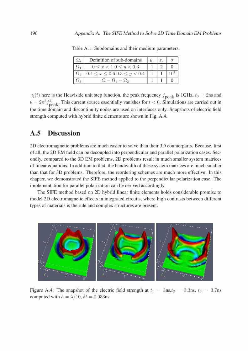
196 Appendix A. The SIFE Method to Solve 2D Time Domain EM Problems
Table A.1: Subdomains and their medium parameters.
Ωi Definition of sub-domains µr εr σ
Ω1 0 ≤ x < 1 0 ≤ y < 0.3 1 2 0
Ω2 0.4 ≤ x ≤ 0.6 0.3 ≤ y < 0.4 1 1 107
Ω3 Ω − Ω1 − Ω2 1 1 0
χ(t) here is the Heaviside unit step function, the peak frequency fpeak is 1GHz, t0 = 2ns and
θ = 2π2f 2
peak. This current source essentially vanishes for t < 0. Simulations are carried out in
the time domain and discontinuity nodes are used on interfaces only. Snapshots of electric field
strength computed with hybrid finite elements are shown in Fig. A.4.
A.5 Discussion
2D electromagnetic problems are much easier to solve than their 3D counterparts. Because, first
of all, the 2D EM field can be decoupled into perpendicular and parallel polarization cases. Sec-
ondly, compared to the 3D EM problems, 2D problems result in much smaller system matrices
of linear equations. In addition to that, the bandwidth of these system matrices are much smaller
than that for 3D problems. Therefore, the reordering schemes are much more effective. In this
chapter, we demonstrated the SIFE method applied to the perpendicular polarization case. The
implementation for parallel polarization can be derived accordingly.
The SIFE method based on 2D hybrid linear finite elements holds considerable promise to
model 2D electromagnetic effects in integrated circuits, where high contrasts between different
types of materials is the rule and complex structures are present.
Figure A.4: The snapshot of the electric field strength at t1 = 3ns,t2 = 3.3ns, t3 = 3.7ns
computed with h = λ/10, δt = 0.033ns

Bibliography
[1] D. M. Sheen, S. M. Ali, M. D. Abouzahra, and J. A. Kong, “Application of the three-
dimensional finite difference time domain method to the analysis of planar microstrip cir-
cuits,” IEEE Trans. on Microwave theory and techniques, vol. 38, pp. 849–857, 1990.
[2] N. P. van der Meijs, “Accurate and efficient layout extraction,” Ph.D. dissertation, Delft
University of Technology, Delft, The Netherlands, January, 1992.
[3] H. Heeb and A. E. Ruehli, “Three-dimensional interconnect analysis using partial element
equivalent circuits,” IEEE Trans. on Microwave Theory and Technology, vol. 39 , No. 11,
pp. 974–982, Nov. 1992.
[4] R. D. Cloux, G. P. F. M. Maas, and A. J. H. Wachters, “Quasi-static boundary element
method for electromagnetic simulation of pcbs,” Philips J. Res., vol. 48, pp. 117–144, 1994.
[5] P. Meuris, W. Schoenmaker, and W. Magnus, “Strategy for electromagnetic interconnect
modeling,” IEEE Trans. on Computer-Aided Design of Integrated Circuits and Systems,
vol. 20, No. 6, pp. 753–762, Jun. 2001.
[6] M. E. Verbeek, “Partial element equivalent circuit (peec) models for on-chip passives and
interconnects,” Eindhoven Univ. of Technology, Tech. Rep., 2002.
[7] B. Song, Z. Zhu, J. D. Rockway, and J. White, “A new surface integral formulation for
wideband impedance extraction of 3-d structures,” in Proc. ICCAD, 2003, pp. 843–847.
[8] K. S. Yee, “Numerical solution of initial boundary value problems involving maxwell’s
equations in isotropic media,” IEEE Trans. on Antennas and Propagation, vol. 14, pp. 302–
307, May 1966.
[9] M. Clemens and T. Weiland, “Discrete electromagnetism with the finite integration tech-
nique,” Progress in Electromagnetic Research, PIER, vol. 32, pp. 65–87, 2001.
197

198 BIBLIOGRAPHY
[10] E. Tonti, “Finite formulation of the electromagnetic field,” Progress in Electromagnetic
Research, vol. 32, pp. 1–44, 2001.
[11] R. Rob, “Note on fdtd method,” Laboratory of Electromagnetic Research, Faculty of Elec-
trical Engineering, Delft University of Technology, Tech. Rep., 2006.
[12] A. Taflove and S. C. Hagness, Computational Electrodynamics: The Finite-Difference
Time-Domain Method, 2nd ed. Artech House Publishers, 2000, ch. 7, Perfectly Matched
Layers Absorbing Boundary Conditions.
[13] B. Cockburn, G. E. Karniadakis, and C.-W. Shu, Eds., Discontinuous Galerkin Methods:
Theory, Compuration and Applications, 1st ed. Springer, May 15, 2000.
[14] D. A.White,Discrete Time Vector Finite Element Methods for SolvingMaxwell’s Equations
on 3D unstructured Grids. Ph.D. dissertation, 1997, pp. 77–78.
[15] J. Webb, “Edge elements and what they can do for you,” IEEE Trans. on Magnetics, vol.
29, Issue: 2, pp. 1460–1465, Mar 1993.
[16] J. Nedelec, “A new family of mixed finite elements in r3,” Numerische Mathematik, vol. 50,
pp. 57–81, 1986.
[17] J. Savage and A. Peterson, “Higher-order vector finite elements for tetrahedral cells,” IEEE
Trans. on Microwave Theory and Techniques, vol. 44, no. 6, pp. 874–879, Jun 1996.
[18] A. Ahagon and T. Kashimoto, “Three-dimensional electromagnetic wave analysis using
high order edge elements,” IEEE Trans. on Magnetics, vol. 31, no. 3, pp. 1753–1756, May
1995.
[19] Z. Ren and N. Ida, “High order differential form-based elements for the computation of
electromagnetic field,” IEEE Trans. on Magnetics, vol. 36, no. 4, pp. 1472–1478, Jul 2000.
[20] T. Yioultsis and T. Tsiboukis, “Development and implementation of second and third or-
der vector finite elements in various 3-d electromagnetic field problems,” IEEE Trans. on
Magnetics, vol. 33, no. 2, pp. 1812–1815, Mar 1997.
[21] B. Bandelier and F. Rioux-Damidou, “Modelling of magnetic fields using nodal or edge
variables,” IEEE Trans. on Magnetics, vol. MAG-26, no. 5, pp. 1644–1646, September
1990.
[22] G. Mur and A. T. de Hoop, “A finite-element method for computing three-dimensional
electromagnetic fields in inhomogeneous media,” IEEE Trans. on Magnetics, vol. 21, Issue:
6, pp. 2188– 2191, 1985.

BIBLIOGRAPHY 199
[23] H. Trabelsi, F. Rioux-Damidou, and B. Bandelier, “Finite element 3d modelling of electro-
magnetic fields with tetrahedral and hexahedral elements,” J. Phys. III, France, vol. 2, pp.
2069–2081, November 1992.
[24] G. Mur, “Finite-element modeling of three-dimensional electormagnetic wave fields, lec-
ture notes for the course et0136,” Laboratory of Electromagnetic Research, Faculty of Elec-
trical Engineering, Delft University of Technology, Tech. Rep., 1996-1997.
[25] ——, “The finite-element modeling of three-dimensional electromagnetic fields using edge
and nodal elements,” IEEE Trans. on antennas and propagation, vol. 41, no. 7, July 1993.
[26] P. Jorna, “Integrated field equations methods for the computation of electromagnetic fields
in strongly inhomogeneous media,” Ph.D. dissertation, Delft University of Technology, Feb
2005.
[27] A. de Hoop and I. Lager, “Domain-integrated field equations approach to static magnetic
field computation - application to some twodimensional configurations,” IEEE Trans. on
Magnetics, vol. 36, no. 4, pp. 654–658, July 2000.
[28] A. T. de Hoop and I. E. Lager, “Static magnetic field computation - an approach based on
the domain-integrated field equations,” IEEE Trans. on magnetics, vol. 34, no. 5, 1998.
[29] I. E. Lager, “Finite element modelling of static and stationary electric and magnetic fields,”
Ph.D. dissertation, Delft University of Technology, 1996.
[30] I. E. Lager and G. Mur, “Generalized cartesian finite elements,” IEEE Trans. on magnetics,
vol. 34, no. 4, pp. 2220–2227, july 1998.
[31] J. Jing, The Finite Element Method in Electromagnetics, 2nd ed. Wiley-IEEE Press, May
2002.
[32] F. Assous, P. Degond, and J. Segre, “Numerical approximation of the maxwell equations in
inhomogeneous media by a p1 conforming finite element method,” Journal of computaional
physics, vol. 128, no. 0217, Feb 1996.
[33] P. Barba, I. Perugia, and A. Savini, “Recent experiences on mixed finite elements for 2d
simulations of magnetic fields,” COMPEL: Int J for Computation and Maths. in Electrical
and Electronic Eng., vol. 17, no. 5, 1998.
[34] K. Sitapati, “Mixed-field finite element computations,” Ph.D. dissertation, Virginia Poly-
technic Institute and State University, 2004.
[35] T. Weiland, “The one-and-only algorithm for em-field computations does not exist,” in
ICEAA: International Conference on Electromagnetics in Advanced Applications, 2009.

200 BIBLIOGRAPHY
[36] Z. Bai, P. Dewilde, and R. Freund, “Reduced-order modeling,” numerical Analysis
Manuscript 02-4-13, Bell Laboratories, 2002.
[37] T. Pals, “Multipole for scattering computations: Spectral discretization, stabilization, fast
solvers,” Ph.D. dissertation, Department of Electrical and Computer Engineering, Univer-
sity of California, Santa Barbara, 2004.
[38] S. Chandrasekaran, M. Gu, and T. Pals, “Fast and stable algorithms for hierarchically semi-
separable representations,” University of California at Santa Barbara, Tech. Rep., April
2004.
[39] P. Dewilde and A.-J. van der Veen, Time-varying Systems and Computations. Kluwer,
1998.
[40] R.Barrett, M. Berry, T.F.Chan, J.Demmel, J.Donato, J.Dongarra, V.Eijhout, R.Pozo,
C.Romine, and H. der Vorst, Templates for the solution of Linear Systems: Building Blocks
for Iterative Methods, SIAM, Ed. Philadelphina, PA: SIAM, 1994.
[41] A. de Hoop, Handbook of Radiation and Scattering of Waves. Academic Press, 1995,
ch. 20, pp. 648–652.
[42] Z. Sheng, R. Remis, and P. Dewilde, “A least-squares implementation of the field integrated
method to solve time domain electromagnetic problems,” CEM-TD, Oct 2007.
[43] ——, “A least-squares implementation of the field integrated method to solve time do-
main electromagnetic problems,” Computational Electromagnetics in Time-Domain, 2007.
CEM-TD 2007. Workshop on, pp. 1–4, 15-17 Oct. 2007.
[44] S.Chandrasekaran, P.Dewilde, W.Lyons, T.Pals, and A.-J. van der Veen, “Fast stable solver
for sequentially semi-separable linear systems of equations,” Octorber 2002.
[45] T. Kailath, “Fredholm resolvents, wiener-hopf equations and riccati differential equations,”
IEEE Trans. on Information Theory, vol. IT-15, p. 6, 1969.
[46] I. Gohberg, T. Kailath, and I. Koltracht, “Linear complexity algorithms for semiseparable
matrices,” Integral Equations and Operator Theory, vol. 8, pp. 780–804, 1985.
[47] Y. Eidelman and I. Gohberg, “On a new class of structured matrices,” Notes distributed
at the 1999 AMS-IMS-SIAM Summer Research Conference, vol. Structured Matrices in
Operator Theory, Numerical Analysis, Control, Signal and Image Processing, 1999.
[48] W. Hackbusch, “A sparse matrix arithmetic based on h-matrices. part 1: Introduction to
h-matrices,” Computing, December 1998.

BIBLIOGRAPHY 201
[49] ——, “A sparse matrix arithmetic based on h-matrices. part i: introduction to h-matrices,”
Computing, vol. 62, no. 2, pp. 89–108, 1999.
[50] ——, “A sparse arithmetic based onH-matrices. part i: Introduction toH-matrices,” Com-
puting, vol. 64, pp. 21–47, 2000.
[51] H. Nelis, “Sparse approximations of inverse matrices,” Ph.D. dissertation, Delft Univ.
Techn., The Netherlands, 1989.
[52] H. Nelis and E. Deprettere, “Approximate inversion of partially specified positive definite
matrices,” inNumerical Linear Algebra, Digital Signal Processing and Parallel Algorithms,
G. Golub and P. van Dooren, Eds. Springer-Verlag, 1991, pp. 559–568.
[53] H. Nelis, E. Deprettere, and P. Dewilde, “Approximate inversion of partially specified posi-
tive definite matrices,” inNumerical Linear Algebra, Digital Signal Processing and Parallel
Algorithms, vol. NATO ASI Series, vol. F70. Springer Verlag, Heidelberg, 1991.
[54] H. Nelis, P. Dewilde, and E. Deprettere, “Inversion of partially specified positive definite
matrices by inverse scattering,” Operator Theory: Advances and Applications, vol. 40, pp.
325–357, 1989.
[55] A. T. de Hoop, Handbook of Radiation and Scattering of Waves, A. Press, Ed. Academic
Press, 1995.
[56] ——, “The mathematics that models wavefield physics in engineering applications - a voy-
age through the landscape of fundamentals,” in Antenas for ubiquitous radio services in a
wireless information society, I. E. Lager and M. Simeoni, Eds., March 2010, pp. 15–26.
[57] ——, “A time-domain uniqueness theorem for electromagnetic wavefield modelling in dis-
persive, anisotropic media.” The Radio Science Bulletin., vol. 305, pp. 17–21, 2003.
[58] A. T. de Hoop, R. F. Remis, and P. M. van den Berg, “The 3d wave equation and its carte-
sian coordinatestretched perfectly matched embedding c a time-domain greens function
performance analysis,” Journal of Computational Physics, vol. 221, pp. 88–105, 2007.
[59] A. Bossavit, “Solving maxwell equations in a closed cavity, and the question of‘spurious
modes,” IEEE Trans. on Magnetics, vol. 26, Issue: 2, pp. 702–705, Mar 1990.
[60] B.-N. Jiang, The Least-Squares Finite Element Method: Theory and Applications in Com-
putational Fluid Dynamics and Electromagnetics (Scientific Computation), Springer, Ed.,
2006.

202 BIBLIOGRAPHY
[61] D. Ioan, I. Munteanu, and C.-G. Constantin, “The best approximation of field effects in
electric circuit coupled problems,” IEEE Trans. on Magnetics, vol. 34, pp. 3210–3213,
1998.
[62] “Doxygen Web page,” 2009, http://www.doxygen.org.
[63] K. van der Kolk and N. van der Meijs, “On the implementation of a 3-dimensional
Delaunay-based mesh generator,” in SCEE 2006 Book of Abstracts, G. Ciuprina and
D. Ioan, Eds., Sinaia, RO, 2006, pp. 171–172, isbn: 978-973-718-520-4.
[64] J. Schoberl, “Netgen - an advancing front 2d/3d-mesh generator based on abstract rules,”
Comput.Visual.Sci, vol. 1, pp. 41–52, 1997.
[65] W. Lyons, “Fast algorithms with applications to pdes,” Ph.D. dissertation, June 2005.
[66] L. Greengard and V. Rokhlin, “A fast algorithm for particle simulations,” J. Comp. Phys.,
vol. 73, pp. 325–348, 1987.
[67] V. Rokhlin, “Applications of volume integrals to the solution of pde’s,” J. Comp. Phys.,
vol. 86, pp. 414–439, 1990.
[68] A. van der Veen, “Time-varying lossless systems and the inversion of large structured ma-
trices,” Archiv f. Elektronik u. Ubertragungstechnik, vol. 49, no. 5/6, pp. 372–382, Sep.
1995.
[69] S. Chandrasekaran, M. Gu, and T. Pals, “A fast and stable solver for smooth recursively
semi-separable systems,” in SIAM Annual Conference, San Diego and SIAM Conference of
Linear Algebra in Controls, Signals and Systems, Boston, 2001.
[70] P. Dewilde and A.-J. van der Veen, “Inner-outer factorization and the inversion of local-
lyfinite systems of equations,” Linear Algebra and its Applications, vol. 313, pp. 53–100,
2000.
[71] T. Pals, “Multipole for scattering computations: Spectral discretization, stabilization, fast
solvers,” Ph.D. dissertation, Department of Electrical and Computer Engineering, Univer-
sity of California, Santa Barbara, 2004.
[72] P. Dewilde, K. Diepold, and W. Bamberger, “A semi-separable approach to a tridiagonal
hierarchy of matrices with application to image flow analysis,” in ProceedingsMTNS, 2004.
[73] S. Chandrasekaran, P. Dewilde, M. Gu, W. Lyons, and T. Pals, “A fast solver for hss rep-
resentations via sparse matrices,” in Technical Report. Delft University of Technology,
August 2005.
BIBLIOGRAPHY 203
[74] S.Chandrasekaran, Z.Sheng, P.Dewilde, M. Gu, and K. Doshi, “Hierarchically semi-
separable representation and dataflow diagrams,” Delft University of Technology, Tech.
Rep., Nov 2005.
[75] S.Chandrasekaran, M.Gu, and T.Pals, “A fast ulv decomposition solver for hierachically
semiseparable representations,” 2004.
[76] P. Dewilde and S. Chandrasekaran, “A hierarchical semi- separable moore-penrose equation
solver,” Operator Theory: Advances and Applications, vol. 167, pp. 69–85, Nov 2006,
birkhauser Verlag.
[77] S.Chandrasekaran, P.Dewilde, M.Gu, W.Lyons, T.Pals, A.-J. van der Veen, and J. Xia, “A
fast backward stable solver for sequentially semi-separable matrices,” September 2005.
[78] W. Lyons and S. Chandrasekaran, “Camlfloat tutorial,” University of California, Santa Bar-
bara, Tech. Rep., 2004.
[79] Z. Sheng, “Hierarchically semi-separable representation and its applications,” Master’s the-
sis, Delft University of Technology, 2006.
[80] W. Lyons, “Fast algorithms with applications to pdes,” Ph.D. dissertation, June 2005.
[81] S. Chandrasekaran, P. Dewilde, M. Gu, W. Lyons, and T. Pals, “A fast solver for hss repre-
sentation via sparse matrices,” Aug. 2005.
[82] S. Chandrasekaran, P. Dewilde, M. Gu, W. Lyons, T. Pals, A.-J. van der Veen, and J. Xia,
“A fast backward stable solver for sequentially semi-separable matrices,” September 2005.
[83] S. Chandrasekaran, M. Gu, and W. Lyons, “A fast and stable adaptive solver for hierachi-
cally semi-separable representations,” April 2004.
[84] Z. Sheng, P. Dewilde, and S. Chandrasekharan, “Algorithms to solve hierarchically
semi-separable systems,” in Operator Theory: Advances and Applications; System
Theory, the Schur Algorithm and Multidimensional Analysis, D. Alpay and V. Vin-
nikov, Eds. Birkhauser Verlag, 2007, vol. 176, pp. 255–294. [Online]. Available:
http://ens.ewi.tudelft.nl/pubs/sheng07operator.pdf
[85] D. Wilton, S. Rao, A. Glisson, D. Schaubert, O. Al-Bundak, and C. Butler, “Potential
integrals for uniform and linear source distributions on polygonal and polyhedral domains,”
IEEE Trans. on Antennas and Propagation, vol. 32, no. 3, pp. 276–281, Mar 1984.
[86] I. Gohberg, M. Kaashoek, and H. Woerdeman, “A maximum entropy principle in the gen-
eral framework of the band method,” J. Functional Anal., vol. 95, no. 2, pp. 231–254, Feb.
1991.

204 BIBLIOGRAPHY
[87] P. Dewilde and E. Deprettere, “The generalized Schur algorithm: Approximation and hier-
archy,” inOperator Theory: Advances and Applications. Birkhauser Verlag, 1988, vol. 29,
pp. 97–116.
[88] ——, “Approximate inversion of positive matrices with application to modeling,” in Mod-
eling, robustness and sensitivity reduction in control systems. Springer, NATO ASI Series,
1987, pp. 212–238.
[89] H. Nelis, “Sparse approximations of inverse matrices,” Ph.D. dissertation, Delft Univ.
Techn., The Netherlands, 1989.
[90] H. Nelis, E. Deprettere, and P. Dewilde, “Approximate inversion of partially specified posi-
tive definite matrices,” inNumerical Linear Algebra, Digital Signal Processing and Parallel
Algorithms, vol. NATO ASI Series, vol. F70. Springer Verlag, Heidelberg, 1991.
[91] S. CHANDRASEKARAN, M. GU, X. S. LI, and J. XIA, “Some fast algorithms for hierar-
chically semiseparable matrices,” Tech. Rep., June 2006.
[92] C. Ashcraft and J. W. H. Liu, “A partition improvement algorithm for generalized nested
dissection,” Boeing Computer Services, Seattle, WA, Tech. Rep. BCSTECH-94-020, 1994.
[93] A. George, “Nested dissection of a regular finite element mesh,” SIAM J. Numer. Anal,
vol. 10, pp. 345–363, 1973.
[94] B. HENDRICKSON and E. ROTHBERG, “Improving the run time and quality of nested
dissection ordering,” SIAM J. SCI. COMPUT., vol. 20, pp. 468–489, 1998.
[95] P. Amestoy, T. A. Davis, and I. S. Duff, “Amd, an approximate minimum degree ordering
algorithm,” ACM Transactions on Mathematical Software, vol. 30, pp. 381–388, Sept 2004.
Samenvatting en Toekomstig Werk
Samenvatting
In dit proefschrift presenteerden we the ‘Surface Integrated Field Equation (SIFE) Method’,
die erin slaagt zowel de statische en stationaire electrische en magnetische veldproblemen op
te lossen, als ook de volle elektromagnetische, en deze zowel in het tijds- als in het frequen-
tiedomein. Deze methode berekent rechtstreeks en simultaan de relevante elektrische en mag-
netische veldsterkten, in tegenstelling tot de traditionele aanpakken die voornamelijk scalaire
en vectorpotentialen uitrekenen. In de methode volgen de veldsterkten direct uit de numerieke
berekeningen, zonder numerieke differentiatie, die een verlies aan nauwkeurigheid in de orde
van de maasgrootte tot gevolg zou hebben. Vergelijkbaar met het werk van Pieter Jorna [26] etr-
effende de berekening van het EM veld in het frequentie domein en zeer verschillend van andere
rekenmethoden gebruikt de SIFE methode de zogenaamde oppervlak-geıntegreerde vergelijkin-
gen van Maxwell. Als aangetoond bevatten die vergelijkingen alle compatibiliteitsrelaties en
gebiedsovergangcondities. Hierdoor behoeven de SIFE vergelijkingen geen speciale behandel-
ing zoals artificiele dissipatie, verschoven roosters of elementen met verschillende orde.
In onze SIFE methode wordt het rekendomein geometrisch gediscretizeerd met behulp van
tetrahedra, ‘hybriede lineaire elementen’ worden geıntroduceerd die zo ontworpen zijn dat de
continue delen van het veld automatisch continu worden voortgezet, maar die toch ruimte laten
voor discontinuiteiten van veldonderdelen die discontinu mogen veranderen. Deze werkwijze
produceert een overgedetermineerd stelsel van lineaire vergelijkingen. We hebben kunnen aan-
tonen dat het systeem inderdaad meer vergelijkingen heeft dan onbekenden (onze formule laat
toe precieze aantal bij voorbaat uit te rekenen). We hebben een studie gemaakt naar de oorzaak
van de overmaat aan vergelijkingen, en hebben aangetoond dat die uitsluitend afkomstig is van
geometrische transformatieoperatoren (Hodge ‘flatten’ en ‘sharp’ operators) in het geometrische
domein en de trapezium regel in het tijdsdomein, terwijl het topologisch deel van de vergelijkin-
gen van Maxwell behouden blijft.
In vergelijking tot andere soorten discretizatie-elementen hebben de hybriede elementen een
aantal voordelen; (1) de benaderingsfout voor het lineaire, hybriede geval is van de orde O(h2)
(met h de gemiddelde maasgrootte); (2) de lineaire, hybriede elementen vormen de juiste combi-
natie van lineaire nodale expansie functies en lineaire ribexpansiefuncties. Zij kunnen gebruikt
worden om vectorfuncties met partiele discontinuiteiten te expanderen, bvb. functies waarvan de
tangentiele componente langs een scheidingsvlak continu is terwijl de normale componente dis-
205
206 Samenvatting en Toekomstig Werk
continu mag varieren; (3) met de lineaire, hybriede expansiefuncties is het makkelijk grenswaar-
den op te leggen die slechts tangentiele waarden bepalen; (4) indien nodig kan de methode ook
gebruikt worden om ingewikkelde gevallen te behandelen waarbij de veldsterkte niet divergen-
tievrij is.
We hebben de voorspelde efficientie en nauwkeurigheid van de de hybriede elementen gev-
erificeerd middels een aantal numerieke experimenten waarvoor analytische oplossingen bek-
end zijn. In al de gevallen die we uitgerekend hebben blijkt de SIFE methode op indruk-
wekkende wijze superieur te zijn. Haar rekencomplexiteit is vergelijkbaar met de conventionele
Galerking methode en de berekeningen convergeren altijd naar de analytische oplossing met
een nauwkeurigheid van de orde O(h2). We hebben bovendien aangetoond dat de methode net
dezelfde hoge nauwkeurigheid bereikt in gevallen met hoog contrast.
Behalve de numerieke verificatie, hebben we de rekennauwkeurigheid van de SIFE methode
vergeleken met die van de bekende ‘Finite Integration Technique (FIT)’ toegepast in het tijds-
domein, en hebben we kunnen aantonen dat de SIFE methode aanzienlijk minder niet-nullen
produceert in de systeemmatrix om dezelfde simulatie nauwkeurigheid te bereiken bij een im-
pliciete tijdsstap methode. Dit betekent dat de SIFE methode minder geheugen behoeft in dit
geval. De SIFE methode produceert bovendien een positief definiete matrix die makkelijk op
te lossen is met een op een interatieve Krylov ruimte gebaseerde stelsel oplosser. Hieruit kun-
nen we concluderen dat de SIFE methode efficienter is dan de FIT methode zowel wat betreft
geheugengebruik als rekentijd. Deze analyse kan ook gebruikt worden als richtlijn voor wanneer
SIFE de voorkeur verdient.
We hebben een volledige implementatie van de SIFE methode genaamd EMsolve3D gemaakt,
gebruikmakend van object-georienteerde programmering en een aantal open bron softare pack-
ages (ook de Galerkin methode hebben we geımplementeerd ter vergelijking). Dit programma
is in staat zowel statische elektrische en magnetische problemen op te lossen als volledig elek-
tromagnetische zowel in het tijds- en frequentie-domein. Voor gebruikersgemak hebben we ook
een grafische ingang geprogrammeerd (GUI) om de oplossers te configureren, de 3D-vermazing
te tonen en de resulaten te visualizeren. Dit pakket moet nog als experimenteel aangemerkt wor-
den, maar we hebben de gebruikte technieken goed gedocumenteerd, adaptief, uitbreidbaar en
patroon-gestuurd (‘pattern based’) uitgevoerd.
Los van het Elektromagnetisch werk, hebben we ook een studie gemaakt van belangrijke
types gestructureerde matrices, dit met het oog op het verbeteren van de prestaties van de nu-
merieke stelseloplossers. In eerste instantie hebben we ons toegelegd op de zgn. ‘Hierarchical
Semi-separable Matrices (HSSMatrices)’. Dit is een belangrijke klasse gestructureerde matrices,
waarvoor de meeste elementaire matrix problemen opgelost kunnen worden met een numerieke
complexiteit die lineair is in het aantal vergelijkingen, en verder nog slechts functie is van struc-
tuurparameters. In het bijzonder hebben we een bewijs gevonden voor het voornaamste resultaat
van de theorie, het oplossen van een stelsel HSS vergelijkingen met lineaire complexiteit, eerst
empirisch voorgesteld in de thesis van Lyon [65]. Het algorithme berekent een expliciete ULV

207
ontbinding van de gegeven matrix en is in staat de Moore-Penrose inverse uit te drukken in
termen van de structuurparameters en met een numerieke complexiteit van dezelfde orde. We
hebben ook de beperkingen van de directe HSS methode bestudeerd, and een algemene strategie
ontwikkeld om de HSS representatie te combineren met een iteratieve methode. Dit hebben we
getest op een aantal relevante voorbeelden. Als resultaat valt te vermelden dat de methode niet
meer goed werkt zodra de voor de methode kenmerkende matrix blokken die buiten de hoofd-
diagonaal vallen niet meer van lage rang zijn (‘not smooth’.) We hebben eveneens een aantal
‘preconditioners’ afgeleid die de HSS structuur hebben en dus in aanmerking komen voor ver-
snelling van de iteratieve oplosser.
Parasitaire capaciteiten van verbindingsdraden op een chip (‘interconnects’) worden steeds
belangrijker naarmate de kenmerkende afmetingen afnemen, en de grootte van de chip gelijk
blijft of toeneemt. Bij sub-micron IC’s waar de bedrading de derde dimensie ingaat en be-
langrijkere laterale oppervlakte heeft moeten 3D capaciteitsmodelleringsmethoden aangewend
worden. In de voorbije jaren hebben een aantal promovendi in Delft hiervoor een nieuwsoortig
lay-out-naar-circuit extractie programma ontwikkeld genaamd SPACE. Het wordt gebruikt om
3D interconnectcapaciteiten nauwkeurig uit te rekenen. Het programma produceert een model
circuit dat naast de de gewone elementen zoals transistors en verbindingen ook nog de parasitaire
capaciteiten bevat en als ingang kan dienen voor een netwerksimulator als SPICE. We hebben
gevonden dat het hierarchisch en adaptief scan programma van SPACE (dat nu bestaat in een 2D
versie), naar 3D kan worden uitgebreid, en we hebben principieel bewijs kunnen leveren van de
mathematische nauwkeurigheid ervan. We hebben deze nieuwe algorithmiek geımplementeerd
in de programmeertaalOcaml en hebben de eigenschappen ervan kunnen waarnemen op een kun-
stmatig, statistisch gegenereerd voorbeeld. Toepassen van deze nieuwe ideeen zou de capaciteit
van SPACE kunnen vergroten.
Toekomstig werk
De modeleringstechnieken en rekenmethoden die in deze thesis zijn voorgesteld hebben vele uit-
breidingsmogelijkheden. Zonder uitputtend te zijn volgt een lijst van mogelijke nieuwe richtin-
gen.
• De SIFE methode kan worden uitgebreid om niet lineaire media te behandelen. In dat
geval moeten ook niet lineaire oplossers worden ontwikkeld.
• Om de nauwkeurigheid van de hybriede elementen methode te verhogen zouden hogere
orde elementen met hogere orde convergentie ontwikkeld kunnen worden.
• Het simulatiepakket EMsolve3D heeft behoefte aan verdere verbeteringen. Een ‘front end
geometry editor’ is zeer gewenst, die in staat is om ingewikkelde layouts te beschrijven.

208 Samenvatting en Toekomstig Werk
De maasgenerator moet verder in het pakket geıntegreerd worden. Ook ‘bug testing’ moet
verder ondernomen worden.
• Een andere belangrijke uitbreiding is het integreren van het pakket met een circuit simula-
tor zodat delen van het circuit met een gewone simulator aangepakt kunnen worden (waar
de golfverschijnselen onbelangrijk zijn) en het hoogfrequente gedeelte dan efficient met de
golfsimulator gedaan kan worden.
• Het opstellen van HSS representaties in concrete simulatieomgevingen is niet voldoende
ondersteund en vraagt aandacht.
• Voorgestelde aanpassingen en uitbreidingen van SPACE zouden het programma van nieuwe
functionaliteit kunnen voorzien.
• Als aangetoond in hoofdstuk 7 is het multi-niveau hierarchische Schur algorithme niet ac-
curaat wanneer de interconnects spaars zijn. Om dit euvel te verhelpen zou een combinatie
van de methode met de snelle Multipole methode ontwikkeld moeten worden zodat dichte
delen door de ene en afstandelijk, spaarse delen door de andere behandeld kunnen worden.

Acknowledgements
My PhD journey would not have been as enjoyable and productive without my colleagues, col-
laborators, friends, and family who were supporting and encouraging me all the time. I would
like to take the opportunity to express my gratitude to all the people who contributed directly or
indirectly to this thesis.
First, I would like to thank my promoter Prof. dr. ir. P. Dewilde who provided me the oppor-
tunity to perform this research and contributed guidance through this project. Although a very
busy professor himself, he took the responsibility as my daily supervisor and was involved in my
work on a week-to-week basis. Even after he moved to Munich, he still made it possible for us
to meet and discuss regularly by either inviting me to Munich or coming back to Delft from time
to time. The generosity and hospitality of him and his wife Anne have made Delft and Munich
so much more enjoyable. He always encouraged and trusted me and gave me much freedom in
doing research. Every encouraging word from him made me more confident and brave. Besides
his scientific support, he was also very helpful in my personal development and gave me many
good advices for life. I also would like to thank him for proof-reading this thesis many times and
translating the summary and propositions in Dutch.
I am also very grateful to my co-promoter Dr. ir. R. F. Remis who always provided me the
valuable and patient guidance whenever I needed them during the whole period of my research
at TU Delft. His expertise on Electromagnetism assisted me on the long battle with Maxwell’s
equations and its intricacies. I also would like to thank him for proof-reading this thesis.
Sincere gratitude is also given to Dr. ir. N. P. van der Meijs from TU Delft for the high quality
scientific discussions, the attention and importance he gave to my research work. I had worked
with him since I was a master student. He was the first person who encouraged me to do research
here. When I asked him for a recommendation letter for PhD applications, he simply replied
“We have a position right now, you should try it”, which was exactly what I did and it lead to
my master thesis and PhD thesis. He was so kind and patient to me and always gave me valuable
suggestions. He helped me reviewing the Object-Oriented Design in Chapter 6, and without his
work on SPACE, Chapter 8 would not exist.
During my PhD study I also had great pleasure to discuss my work with Prof. dr. W. H. A.
Schilders from Technische Universiteit Eindhoven, Dr. W. Schoenmaker from Magwel NV, Prof.
dr. ir. A. J. van der Veen from TU Delft, Prof. dr. ir. A. T. de Hoop from TU Delft, Prof. dr. S.
Chandrasekaran from University of California, Santa Barbara, Prof. Ming Gu from University of
California, Berkeley and Prof. Daniel Ioan from “Politehnica” University of Bucharest. I would
209

210 Acknowledgements
like to express my sincere appreciation to all of them for their contributions, specially Prof.
dr. S. Chandrasekaran whose excellent work on Hierarchically Semi-Separable systems inspired
Chapter 7, Prof. Daniel Ioan for offering me a Marie-Curie research fellowship in “Politehnica”
University of Bucharest and Prof. Ming Gu for inviting me for a visit to University of California,
Berkeley.
I would like to thank all my colleagues at the Circuit and System group for making the 17th
floor a friendly and enjoyable environment to work in. Specially I would like to thank my office-
mate Kees-Jan van der Kolk for helping me out with programming problems, providing valuable
discussions and bringing nice gadgets to control humidity and fresh air in the office.
My gratitude also goes to the secretary in CAS group, Laura Bruns. She has been very kind
and helpful. She helped me through a large number of forms and procedures at many occasions.
Without her, I would have lost in formalities and procedures by now.
It was difficult for me to live far away from my family, but my Chinese friends in the Nether-
lands made me feel at home. My life in the Netherlands would not have so much fun without
any of them. Xinyang Wang, Yanxia Zhang, Bingjie Fu, Zhoujian, Zhoubo, Jihan Li and many
others.
Finally, I give my deepest gratitude to my family. I would like to thank my parents Qilin
Sheng and Xiaoping Liu for encouraging and supporting me during all my life. I would like to
thank my wife Shanfeng Jiang for giving me everyday strength, happiness, and, most important,
love.
Zhifeng Sheng
Hoevelaken, The Netherlands
May 24, 2010

About the Author
Zhifeng Sheng was born on the 19th of October, 1982 in Changsha, Hunan Province, P.
R. China. From 2000 to 2004, he studied Computer Science and received his Bachelor degree
from the talented program in Central South University, Changsha, China. In August 2004, he
moved to the Netherlands. From 2004 to 2006, he studied Computer Engineering and received
his Master of Science degree with honors (cum laude) at Delft University of Technology. In June
2006, he was appointed as a Ph.D student in the Circuit and Systems group at Delft University
of Technology. Since then, he has been working on numeric analysis, modeling and simulation,
which involved mathematics, physics, and software engineering. From December 2008 to April
2009, he was appointed as a Marie Curie research fellow in the Numerical Methods Laboratory at
“Politehnica” University of Bucharest, Romania. At this moment, he continues his adventure on
numeric modeling and simulation by developing medical visualization and simulation software
at the high-tech start-up company Virtual Proteins B.V, Eindhoven, the Netherlands.
Publications
• Z. Sheng; P. Dewilde; N. van der Meijs “3D Capacitance extraction based on multi-level
hierarchical Schur algorithm” In 20th annual workshop on circuits, systems and signal
211

212 About the Author
processing–ProRISC, Veldhoven, STW, pp. 551-555, November 2009. ISBN 978-90-
73461-62-8.
• Z. Sheng; P. Dewilde; R.F. Remis “Surface integrated field equations method for comput-
ing 3D static and stationary electric and magnetic fields” In ICEAA 2009 Proceedings of
the 11th Int. Conf. on Electromagnetics in Advanced Applications, Turin (Italy), IEEE, pp.
388-391, October 2009. ISBN 1-4244-3385-8.
• Z. Sheng; P. Dewilde “An Electromagnetic simulation package: EMsolve3D” inDATE, the
Design, Automation and Test Conference and Exhibition, University Booth, Nice, France,
April 2009.
• Z. Sheng; P.M. Dewilde; R. Remis “Surface Integrated Field Equations Method for Solv-
ing 3D Electromagnetic Problems” In Janne Roos and Luis R.J. Costa (Ed.), Scientific
Computing in Electrical Engineering SCEE 2008, Springer, pp. 77-84, 2008.
• Z. Sheng; N.P. van der Meijs “Surface integrated field equations method for computing
3D static and stationary electric and magnetic fields” In 19th annual workshop on circuits,
systems and signal processing–ProRISC, Veldhoven, STW, November 2008.
• Z. Sheng; P.M. Dewilde; S. Chandrasekharan “Algorithms to solve hierarchically semi-
separable systems” In D. Alpay; V. Vinnikov (Ed.),Operator Theory: Advances and Appli-
cations; System Theory, the Schur Algorithm and Multidimensional Analysis, Birkhauser
Verlag, pp. 255-294, 2007. DOI 10.1007/978-3-7643-8137-0 5.
• Z. Sheng; R. Remis; P.M. Dewilde “A least-squares implementation of the field integrated
method to solve time domain electromagnetic problems” In IEEE Workshop on Compu-
tational Electromagnetics in Time-Domain, Perugia (IT), IEEE, pp. 1-4, October 2007.
ISBN 978-1-4244-1170-2, DOI 10.1109/CEMTD.2007.4373514.
• Z. Sheng; P.M. Dewilde; R.F. Remis “The field integrated method to solve time domain
electromagnetic problems” In IEEE/ProRISC workshop on Circuits, Systems and Signal
Processing, Veldhoven (NL), IEEE, November 2007. ISBN 978-90-73461-49-9.
• Z. Sheng; P. Dewilde; N. van der Meijs “Iterative solution methods based on the hierarchi-
cally semi-separable representation” In Proc. 17th annual workshop on Circuits, Systems
and Signal Processing (ProRISC), Veldhoven (NL), pp. 343-349, November 2006.
• Z. Sheng; R.F. Remis; A.T. de Hoop; P.M. Dewilde “An exploration of the integrated field
equations method for Maxwell s equation” In G. Ciuprina; D. Ioan (Ed.), SCEE 2006 Book
of Abstracts, 2006. ISBN: 978-973-718-520-4.

213
Oral Presentations
• “Surface integrated field equations method for computing 3D static and stationary elec-
tric and magnetic fields” ; in International Conference on Electromagnetics in Advanced
Applications, Turin (Italy), IEEE, October 2009.
• “Surface integrated field equations method for computing electromagnetic fields”; in Ma-
trix Computations & Scientific Computing Seminar, University of California, Berkeley,
USA, March 2009.
• “Surface Integrated Field Equations Method for Solving 3D Electromagnetic Problems”;
in Scientific Computing in Electrical Engineering, Helsinki University of Technology Es-
poo, Finland, September 2008.