accurate modeling of ionospheric electromagnetic fields
TRANSCRIPT
AFRL-RV-HA-TR-2009-1055
Accurate Modeling of Ionospheric Electromagnetic Fields Generated by a Low Altitude VLF Transmitter Steven A. Cummer Jingbo Li Duke University Box 90291 Durham, NC 27708 Final Report 31 March 2009
Approved for public release; distribution unlimited.
AIR FORCE RESEARCH LABORATORY Space Vehicles Directorate 29 Randolph Road AIR FORCE MATERIEL COMMAND HANSCOM AFB, MA 01731-3010

AFRL-RV-HA-TR-2009-1055 Using Government drawings, specifications, or other data included in this document for any purpose other than Government procurement does not in any way obligate the U.S. Government. The fact that the Government formulated or supplied the drawings, specifications, or other data, does not license the holder or any other person or corporation; or convey any rights or permission to manufacture, use, or sell any patented invention that may relate to them. This report is published in the interest of scientific and technical information exchange and its publication does not constitute the Government’s approval or disapproval of its ideas or findings. This technical report has been reviewed and is approved for publication. / signed / / signed / Arthur J. Jackson James T. Dodd, Acting Chief Contract Manager Space Weather Center of Excellence Qualified requestors may obtain additional copies form the Defense Technical Information Center (DTIC). All other requests shall be referred to the National Technical Information Service. If your address has changed, if you with to be removed from the mailing list, or if the addressee is no longer employed by your organization, please notify AFRL/RVIM, 29 Randolph Rd., Hanscom AFB, MA 01731-3010. This will assist us in maintaining a current mailing list. Do not return copies of this report unless contractual obligations or notices on a specific document require that it be returned. For Unclassified, limited documents, destroy by any means that will prevent disclosure of the contents or reconstruction of the document.
REPORT DOCUMENTATION PAGE Form Approved
OMB No. 0704-0188 Public reporting burden for this collection of information is estimated to average 1 hour per response, including the time for reviewing instructions, searching existing data sources, gathering and maintaining the data needed, and completing and reviewing this collection of information. Send comments regarding this burden estimate or any other aspect of this collection of information, including suggestions for reducing this burden to Department of Defense, Washington Headquarters Services, Directorate for Information Operations and Reports (0704-0188), 1215 Jefferson Davis Highway, Suite 1204, Arlington, VA 22202-4302. Respondents should be aware that notwithstanding any other provision of law, no person shall be subject to any penalty for failing to comply with a collection of information if it does not display a currently valid OMB control number. PLEASE DO NOT RETURN YOUR FORM TO THE ABOVE ADDRESS.
1. REPORT DATE (DD-MM-YYYY) 31-03-2009
2. REPORT TYPE
Scientific, Final3. DATES COVERED (From - To)
02-08-2006 – 31-12-20084. TITLE AND SUBTITLE
Accurate Modeling of Ionospheric Electromagnetic Fields Generated by a 5a. CONTRACT NUMBER
FA8718-05-C-0052 Low Altitude VLF Transmitter 5b. GRANT NUMBER
5c. PROGRAM ELEMENT NUMBER
63278E 6. AUTHOR(S)
Steven A. Cummer 5d. PROJECT NUMBER
DARP Jingbo Li 5e. TASK NUMBER
RR 5f. WORK UNIT NUMBER
58 7. PERFORMING ORGANIZATION NAME(S) AND ADDRESS(ES)
Duke University 130 Hudson Hall, Box 90291 Durham, NC 27708
8. PERFORMING ORGANIZATION REPORT NUMBER
9. SPONSORING / MONITORING AGENCY NAME(S) AND ADDRESS(ES) 10. SPONSOR/MONITOR’S ACRONYM(S)
Air Force Research Laboratory 29 Randolph Road Hanscom AFB, MA 01731-3010
AFRL/RVBXR
11. SPONSOR/MONITOR’S REPORT NUMBER(S)
AFRL-RV-HA-TR-2009-105512. DISTRIBUTION / AVAILABILITY STATEMENT Approved for public release; distribution unlimited.
13. SUPPLEMENTARY NOTES
14. ABSTRACT
The goal of this project is to accurately predict the high altitude wave energy generated by low altitude VLF sources. We applied full-wave finite difference numerical models of the electromagnetic fields in both time and frequency domain to compute the VLF energy injected through an arbitrary and therefore realistic ionosphere for a source located anywhere on the globe. A 2D finite difference time domain (FDTD) code has been validated in various methods and proved to converge to the correct answer. A complete convergence test shows the conditions under which the code generated quantitatively correct results. Comparisons with results from this time domain code show that our frequency domain code gives answers in quantitative agreement but is about 40 times faster for single frequency computations. With these two models developed, we analyze in detail the power flux at 120 km altitude produced by the NML ground transmitter. To further study the dependence of wave energy on Earth’s magnetic field, we also analyze the high altitude wave energy and ionospheric absorption for transmitters located at all latitudes. Our results can be used to predict the high altitude VLF power produced by a nearly arbitrary ground-level VLF transmitter. 15. SUBJECT TERMS
Finite-difference-time-domain method Wave energy injection Ionospheric absorption Radiation belt dynamics 16. SECURITY CLASSIFICATION OF:
17. LIMITATION OF ABSTRACT
18. NUMBER OF PAGES
19a. NAME OF RESPONSIBLE PERSON
Arthur J. Jackson a. REPORT
UNCL b. ABSTRACT UNCL
c. THIS PAGE
UNCL UNL
19b. TELEPHONE NUMBER (include area code)
Standard Form 298 (Rev. 8-98)Prescribed by ANSI Std. 239.18


iii
CONTENTS
List of Figures...............................................................................................................iv List of Tables ...............................................................................................................vii 1. Summary and Accomplishments...........................................................................1 2. General Approach .................................................................................................2 3. Technical Approach...............................................................................................3
3.1 Governing Equations.........................................................................................3
3.2 2D Cylindrical Symmetric FDTD Modeling.....................................................5
3.3 Time Harmonic Modeling........................................................................10 4. Model Validation .................................................................................................14
4.1 FDTD comparison with LWPC.......................................................................14
4.2 FDTD Comparison with High Altitude Rocket Data .....................................15
4.3 FDTD Convergence Test .................................................................................19
4.4 FDFD Comparison to FDTD ...........................................................................26 5. Results ......................................................................................................................34
5.1 Upward VLF Power from the NML Transmitter ..........................................34
5.2 High Altitude VLF Power Versus Latitude ....................................................38 REFERENCES ............................................................................................................47

iv
List of Figures
Figure 1. 2D cylindrical symmetric computation domain (left) and FDTD grid layout (right). .....................................................................................................................5
Figure 2. Diagrams of Earth’s magnetic field radial component: 3D model (left) and 2D
cylindrical model (right). .........................................................................................6 Figure 3. FDTD simulated high altitude (90 km) electric fields 60 km away from a
lightning source in the south and north directions. The codip angle is 20 degrees.....7 Figure 4. FDTD simulation results of all the 6 field components caused by a short
dipole with unit current. The transmitting frequency is 10 kHz. The earth magnetic field is vertical. ........................................................................................................8
Figure 5. FDFD simulation results of all the 6 field components caused by a short
dipole with unit current. The transmitting frequency is 10 kHz and the Earth magnetic field is vertical. .......................................................................................11
Figure 6. Schematic of computation domain in the segmented approach .....................11 Figure 7. Top left and right: The vertical electric field distribution from a 20 kHz high
latitude transmitter in two adjacent segments using the segmented approach. Bottom left and right: Comparison of the fields computed using 5 segments (left) and one segment (right). ........................................................................................13
Figure 8. Comparisons of LWPC and FDTD predictions of low altitude 25.2 kHz vertical
electric fields as a function of range from the transmitter. Results for two distinct propagation directions relative to Earth’s magnetic field are presented, both of which yield excellent agreement. Based on the three validations made above to both experimental data and LWPC model, we can conclude that the FDTD is capable to produce reliable results. .........................................................................................15
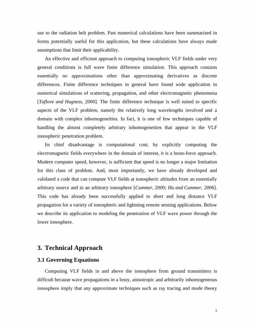
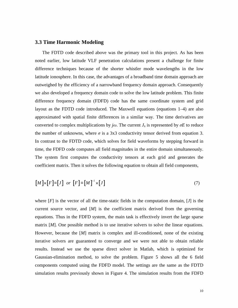
Figure 9. The rocket trajectory for the daytime rocket and the flight geometry for both
rockets. ..................................................................................................................16 Figure 10. Electron density profiles, (left) daytime and (right) nighttime .......................16 Figure 11. Comparison of measured and simulated horizontal magnetic field from the
daytime rocket. Simulations were run with a 300 m grid size. .............................17 Figure 12. Comparison of measured and simulated horizontal magnetic field from the
nighttime rocket. Simulations were run with a 300 m grid size............................18 Figure 13. FDTD convergence for f = 10 kHz, Mlat = 80 degrees..................................21

v
Figure 14. FDTD convergence for f = 10 kHz, Mlat = 50 degrees..................................21 Figure 15. FDTD convergence for f = 10 kHz, Mlat = 30 degrees..................................22 Figure 16. Average error of results from 250 m grid size to the best estimate at different
latitudes for transmission frequency of 10 kHz. The blue stars represent errors at high altitude and the red stars represent the errors at low altitude. ..........................23
Figure 17. FDTD convergence for f = 25 kHz, Mlat = 80 degrees..................................24 Figure 18. FDTD convergence for f = 25 kHz, Mlat = 50 degrees..................................24 Figure 19. FDTD convergence for f = 25 kHz, Mlat = 30 degrees..................................25 Figure 20. Average error of simulation results from 250 m spacing to the best estimate at
the different latitudes for transmission frequency of 25 kHz. The blue stars represent errors at high altitudes and the red stars represent the errors at low altitudes. .........26
Figure 21. FDFD convergence for f = 10 kHz, Mlat =80 degrees. ..................................28 Figure 22. FDFD convergence for f = 10 kHz, Mlat = 50 degrees. .................................28 Figure 23. FDFD convergence for f = 10 kHz, Mlat = 30 degrees. .................................29 Figure 24. The relative error between FDFD and FDTD best estimates for high and low
altitude fields with a signal frequency of 10 kHz....................................................30 Figure 25. FDFD convergence of f= 25 kHz, Mlat = 80 degrees. ...................................31 Figure 26. FDFD convergence of f = 25 kHz, Mlat = 50 degrees. ..................................32 Figure 27. FDFD convergence for f = 25 kHz, Mlat = 30 degrees. .................................32 Figure 28. Relative difference between FDFD and FDTD results for low and high
altitudes simulations for a 25 kHz signal. ...............................................................33 Figure 29. The spatial distribution in an east-west plane for all 6 electromagnetic field
components in cylindrical coordinates produced by a 25.2 kHz transmitter at the location of NML. A fully inhomogeneous background magnetic field is included which is responsible for the visible east-west anisotropy........................................35
Figure 30. Convergence analysis of the upward VLF power at 120 km altitude from the
NML transmitter. The computation with 1000 m grid size underpredicts the power, but the 500 and 250 m computations are almost identical, indicating that this is the converged and therefore correct answer. ................................................................36
vi
Figure 31. A full geographic distribution of the upward power flux at 120 km altitude from the NML transmitter......................................................................................37
Figure 32. Calculation of the spatial distribution of the wave vector direction at 120 km
altitude from the NML transmitter. ........................................................................38 Figure 33. Vertical power flux and power absorption at 120 km altitudes for 80, 50 and
30 degree latitudes. The transmission signal is 10 kHz. The left panels show the vertical power flux. The right panels show the ration between the vertical power flux at 120 km altitude and the horizontal power flux at ground. ...................................40
Figure 34. Total power flux in a computation domain of 500 km x 120 km for
propagation path of 45 degree (north east) and 225 degree (south west). The color intensity and the arrow on each plot represent the magnitude and direction of power flux........................................................................................................................41
Figure 35. Vertical Power Flux and absorption rate at 25 kHz. Left panels show the
vertical power flux at three latitudes. Right panels show the ratio between high altitude vertical power flux and low altitude horizontal power flux. .......................42
Figure 36. Average upward power flux per kW transmitted at 120 km altitude. Top: f =
10 kHz. Bottom: f = 25 kHz................................................................................43 Figure 37. Average ratio of high altitude average upward power density to average
outward power density at ground. Top: f = 10 kHz. Bottom: f = 25 kHz..............45

vii
List of Tables
Table 1. Computation time of C code and Matlab code....................................................9 Table 2. Computation times for FDTD and FDTD on Matlab platform..........................14

1
1. Summary and Accomplishments
The main objective of this project is to apply a full-wave electromagnetic field model
to predict the injection of wave energy produced by a low altitude very low frequency
(VLF) transmitter through an arbitrary and therefore realistic ionosphere. Our specific
task is to deliver accurate predictions of high altitude electromagnetic fields and wave
energy injection. Accurate prediction of high altitude wave energy injection by
low-altitude VLF wave transmission is a challenging but essential step towards accurate
modeling of the impact of man-made VLF transmissions on natural radiation belt
dynamics. The technical challenge lies in simulating propagation in a lossy, anisotropic
and arbitrarily inhomogeneous ionosphere, for which approximate techniques such as ray
tracing do not apply.
Our technical approach is to develop a full-wave numerical model to simulate wave
power injected into the ionosphere from a ground-level VLF transmitter. The main
advantage of a finite difference-based approach is its ability to compute high altitude
fields in arbitrary ionospheres, including the influence of Earth’s magnetic field, with no
implicit approximations. A 2D Finite Difference Time Domain (FDTD) model and a
Finite Difference Frequency Domain (FDFD) model have been developed to accomplish
the task. The FDTD model has been validated with experimental data including
satellite-measured NML transmitter VLF electric fields and rocket-based measurements
of VLF electric and magnetic fields in the lower ionosphere. The FDTD results are also
consistent with the well-validated LWPC mode theory propagation model. The FDFD
code was validated with the FDTD model.
We have expended significant effort in understanding the convergence of our
simulations and thus also quantitatively bounding the absolute errors in the results. We
have run a series of simulations using parameters corresponding to magnetic latitude
from 0 degree to 90 degree to examine the convergence of the models in all the latitude.
Finite difference simulations are guaranteed to eventually converge to the correct answer
as this grid spacing is reduced, provided the code is stable, but it is not always easy to
know what grid spacing is required to maintain errors below a specified level. We have
found that for insufficiently small grid sizes, the low altitude fields can be computed
2
correctly while the high altitude fields are dramatically incorrect. Our results show that
both of the models converge properly with spacing size of 250 m (or even 500 m) at mid
to high latitudes. At low latitudes, the FDTD model exhibits variations that make it
difficult to determine a reliable answer, but the FDFD model converges properly. The
convergence in all cases shows second-order accuracy, as expected, which means that
correct answers can be estimated by extrapolating the convergence to its limit.
We have applied both models to compute the vertical power flux at high altitude (120
km) and the effective absorption, defined as the ratio of the high altitude
upward-propagating power to the low altitude outward-propagating power. Our results
show that the high altitude power flux and the effective absorption are strong functions of
the direction of wave propagation with respect to the background magnetic field. At
different latitudes, the power flux in the southward direction, effectively close to
antiparallel to the background magnetic field, is roughly constant. The power flux in the
northward direction, effectively close to perpendicular to the background magnetic field,
is much lower and is a strong function of both latitude and signal frequency. For a 10 kHz
signal, the absorption varies from –12 dB at magnetic equator to –51 dB at 10 degrees
latitude. For 25 kHz signal, the absorption rate varies from –15 dB to –82 dB for the same
latitude range. These results are summarized in a series of plots at the end of this report.
2. General Approach
Predicting the wave power injected into the magnetosphere from a ground-level VLF
or lower frequency transmitter is an essential component in modeling radiation belt
dynamics. But accurately computing VLF power penetration through the ionosphere is
not easy. Ray tracing, an effective technique for modeling VLF power flow in the
magnetosphere, is not a good approximation because the ionosphere changes significantly
on the scale of a VLF wavelength. Consequently, wave reflection, mode conversion, and
other full-wave effects that ray tracing generally neglects are important. Full-wave mode
theory techniques [e.g., Pappert and Ferguson, 1986] are effective for reliably computing
subionospheric fields produced by VLF transmitters. But mode theory techniques are
difficult to apply above approximately 60–70 km for realistic ionospheres in which the
parameters are not exponentially varying. This upper altitude is too low to be of direct
3
use to the radiation belt problem. Past numerical calculations have been summarized in
forms potentially useful for this application, but these calculations have always made
assumptions that limit their applicability.
An effective and efficient approach to computing ionospheric VLF fields under very
general conditions is full wave finite difference simulation. This approach contains
essentially no approximations other than approximating derivatives as discrete
differences. Finite difference techniques in general have found wide application in
numerical simulations of scattering, propagation, and other electromagnetic phenomena
[Taflove and Hagness, 2000]. The finite difference technique is well suited to specific
aspects of the VLF problem, namely the relatively long wavelengths involved and a
domain with complex inhomogeneities. In fact, it is one of few techniques capable of
handling the almost completely arbitrary inhomogeneities that appear in the VLF
ionospheric penetration problem.
Its chief disadvantage is computational cost; by explicitly computing the
electromagnetic fields everywhere in the domain of interest, it is a brute-force approach.
Modern computer speed, however, is sufficient that speed is no longer a major limitation
for this class of problem. And, most importantly, we have already developed and
validated a code that can compute VLF fields at ionospheric altitudes from an essentially
arbitrary source and in an arbitrary ionosphere [Cummer, 2000; Hu and Cummer, 2006].
This code has already been successfully applied to short and long distance VLF
propagation for a variety of ionospheric and lightning remote sensing applications. Below
we describe its application to modeling the penetration of VLF wave power through the
lower ionosphere.
3. Technical Approach
3.1 Governing Equations
Computing VLF fields in and above the ionosphere from ground transmitters is
difficult because wave propagations in a lossy, anisotropic and arbitrarily inhomogeneous
ionosphere imply that any approximate techniques such as ray tracing and mode theory

4
for wave simulation are not accurate. Our technique approach is to solve all the field
components radiated by a dipole source with full Maxwell equations and vector electric
current in magnetized cold plasma, namely
0HEt
µ!
"# = $!
(1)
0 totEH Jt
!"
#$ = % +"
(2)
20( )
| |n
n b n E pJ qJ J b Et q
! " # "$
+ = % +$
(3)
tot nJ J= ! (4) where E, H, and Jn are the vector electric field, magnetic field and electric current
induced by different species of particles in the ionosphere; ωp is the local plasma
frequency; ωb is the local gyrofrequency; υ is the local collision frequency; and bE is the
unit vector pointing in the direction of Earth’s magnetic field [Budden, 1985]. All of cold
plasma magnetoionic theory is contained in these equations and thus all relevant physics
of linear electromagnetic waves are automatically included in this simulation. For
example, the complicated Appleton-Hartree refractive index formula is derived directly
from the time harmonic equivalent of the above equations. Both electron and ion effects
are included in our model by separately computing the current from each particle species
through equations of the same form. Thus the task of modeling becomes solving the
above governing equations everywhere in the computation domain. We numerically solve
the governing equations by approximating the curl operator derivatives as the finite
discrete difference as
0
20 0( / 2) ( / 2)df ( )dz z z
f z z f z z O zz=
+ ! " "!= + !
! (5)
where Δz is the spatial resolution and f(z) is the field quantity. The error of this
approximation is proportional to the second order of the spatial resolution. Thus the
solution should exhibit second order convergence to the true result with an error that
decreases by a factor of 4 for every factor of 2 reduction in the spatial resolution. With

5
this approach, we can solve the problem in either the time domain or the frequency
domain. Both approaches are described and applied in this report.
3.2 2D Cylindrical Symmetric FDTD Modeling
Our primary computational model is expressed in 2D azimuthally symmetric
cylindrical coordinates. Figure 1 shows the computational domain (left) and the grid
layout used in our model. The computational domain is a 2D cylinder and is symmetric in
the azimuthal direction. The bottom part is the ground, which can be treated as a perfect
electrical conductor (PEC) boundary for VLF frequencies. The ionosphere is defined by
the number density of different charged particles and their collision frequencies. The
vertical and radial outer regions are set as perfect matched layers as the absorbing
boundaries [Cummer, 2003]. A vertical electric dipole source is located in the center of
the cylindrical domain with adjustable length and predefined current waveform. The
entire computation domain is first mapped into discrete grids with desired spatial
resolution. Then time iterations are to solve the field quantities at all the grids and all time
steps. At each time step, the curl operations in the Maxwell equations are discretized with
equation (5).
Figure 1. 2D cylindrical symmetric computation domain (left) and FDTD grid layout (right).

6
For example, for the Er, Ez and Hφ components in the TM polarization, the original
Maxwell equation will be transferred into the difference equation
0 0
0( / 2) ( / 2) ( / 2) ( / 2)
r z
new oldr r z z
HE EHEt z r t
H HE z z E z z E r r E r rz r t
!
! !
µ µ
µ
"" ""#$ = % & % = %
" " " "
%+ ' % %' + ' % %'& + = %
' ' '
(6)
As mentioned earlier, this method exhibits second order convergence for the fields
computed.
Comparing to fully 3D simulations, 2D simulations are vastly less time consuming
and save computational resources. However, one main difference between our 2D
cylindrical model and a fully 3D model is how the background magnetic field is treated.
The Earth’s magnetic field has a significant impact on the radio wave behavior in the
ionosphere because the electric currents caused by the charged particles are affected by
the background magnetic field (see equation 4). In reality, the background magnetic field
is not azimuthally symmetric and thus cannot be simulated exactly in 2D cylindrical
coordinates used in our FDTD code. However, we can make a reasonable approximation
in which the 1D background magnetic field variation along the propagation path is
rotated to provide azimuthal symmetry. Figure 2 shows how this conversion from 3D to
2D is done.
Figure 2. Diagrams of Earth’s magnetic field radial component: 3D model (left) and 2D cylindrical model (right).

7
Since it is difficult to analytically estimate the magnitude of the error incurred by this
background magnetic field approximation, a 3D model simulation is the best way to test
the accuracy of this assumption. Therefore, we have developed a fully 3D version of this
code, which is much slower to run but more accurate in representing the Earth’s magnetic
field. We used the 3D model in limited runs to validate the approximations made in the
2D model and therefore to ensure its accuracy. Figure 3 shows the simulated electric field
at 90 km altitude at two different locations, which are 60 km north (left panel) and south
(right panel) to a broadband lightning source. The background magnetic field has a codip
angle of 20 degrees. The different waveform shapes in the two directions shows the
anisotropy of the medium. In both simulations, the electric field from the 3D model
agrees very well with that from the 2D model. Therefore, a single 2D FDTD run is
equivalent to a 3D FDTD run.
Figure 3. FDTD simulated high altitude (90 km) electric fields 60 km away from a lightning source in the south and north directions. The codip angle is 20 degrees.
Our 2D FDTD model is capable of computing the time domain signal at any point in
the computational domain. However, it is not realistic or efficient to save all these
waveforms, especially for long time sequences and large computation domains.
Furthermore, only certain frequencies are of interest for computing the VLF transmitter
power in this application. Thus instead of storing all the time domain fields at each grid,
we only compute and restore the complex fields of certain frequencies specified by the

8
user. This can be achieved by incorporating the Discrete Fourier Transform (DFT)
algorithm into the FDTD code. At each time step, after updating the time domain fields,
the code updates the complex field with DFT method. This way, a continuously updated
complex number is saved at each grid point instead of a full time domain signal. Since
only one equation is added to each frequency component in the code, running the DFT
algorithm is fast and almost does not appreciably increase the total computation time.
Figure 4 shows all the 6 field components produced by a short dipole with unit current
amplitude at 10 kHz. The computation domain is 500 km (horizontal) by 120 km
(vertical) and the background magnetic field is in the vertical direction. At low altitudes,
the strongest fields are Ez and Bφ, the primary components produced by a vertical electric
dipole source. Other components generated only through the anisotropy of the ionosphere
are present at smaller amplitudes.
Figure 4. FDTD simulation results of all the 6 field components caused by a short dipole with unit current. The transmitting frequency is 10 kHz. The earth magnetic field is vertical.
Various versions of our VLF propagation model have all been initially developed on
the Matlab platform because debugging and visualization are much easier on this

9
platform than with a compiled code. Matlab’s vector operators are also relatively fast and
thus the speed penalty paid for the platform simplicity is not enormous. However, for this
effort we need to run many instances of these codes for different propagation paths, and
any speed up that we can achieve will be useful. Thus the original Matlab code was been
converted to C language. Our C code uses threads for parallel processing in order to take
advantage of the multiple CPU architecture of most modern computers. This feature can
easily be removed on machines that do not support multithreading, but it provides
significant speedup on processors that do support this feature. Second, we recognized that
the most time consuming part of the program is the section that updates field quantities at
each time step. Consequently, the data used in this section is organized in memory in
such a way to increase data localization and consequently decrease cache misses (i.e. the
need to bring data from RAM to the CPU cache). More specifically, all field matrices and
coefficients are saved in adjacent regions of memory, each matrix is accessed
sequentially, i.e. we avoid accessing elements that are placed too far away from each
other in memory. Third, we minimized the use of floating point arithmetic as much as
possible by keeping partial results used often in the code in temporary variables.
Table 1. Computation time of C code and Matlab code Stepsize (m) Matlab (hr) C code (hr) 1000 19.8 0.7 500 162.7 4.2 250 ~1300 45.4
The comparison of computation time between C and Matlab code is shown in Table
1. Some comments about the conditions of this test are in order. These tests were run on a
dual core 2.8 GHz Xeon processor machine. Matlab only uses a single core, while the C
code is multithreaded. Consequently some of the speed up comes from more efficient use
of existing resources. The speedup factor is very dependent on the size of the
computational domain because Matlab’s efficiency appears to drop as memory use
becomes high. Thus the observed 30x drops to about 10x for smaller computational
domains. However, this 30x speedup is for the conditions under which we actually use
this code, i.e. large computational domains. Consequently, the practical improvement we
have realized through this code conversion effort is in fact a factor of 30.
10
3.3 Time Harmonic Modeling
The FDTD code described above was the primary tool in this project. As has been
noted earlier, low latitude VLF penetration calculations present a challenge for finite
difference techniques because of the shorter whistler mode wavelengths in the low
latitude ionosphere. In this case, the advantages of a broadband time domain approach are
outweighed by the efficiency of a narrowband frequency domain approach. Consequently
we also developed a frequency domain code to solve the low latitude problem. This finite
difference frequency domain (FDFD) code has the same coordinate system and grid
layout as the FDTD code introduced. The Maxwell equations (equations 1–4) are also
approximated with spatial finite differences in a similar way. The time derivatives are
converted to complex multiplications by jω. The current Jn is represented by σE to reduce
the number of unknowns, where σ is a 3x3 conductivity tensor derived from equation 3.
In contrast to the FDTD code, which solves for field waveforms by stepping forward in
time, the FDFD code computes all field magnitudes in the entire domain simultaneously.
The system first computes the conductivity tensors at each grid and generates the
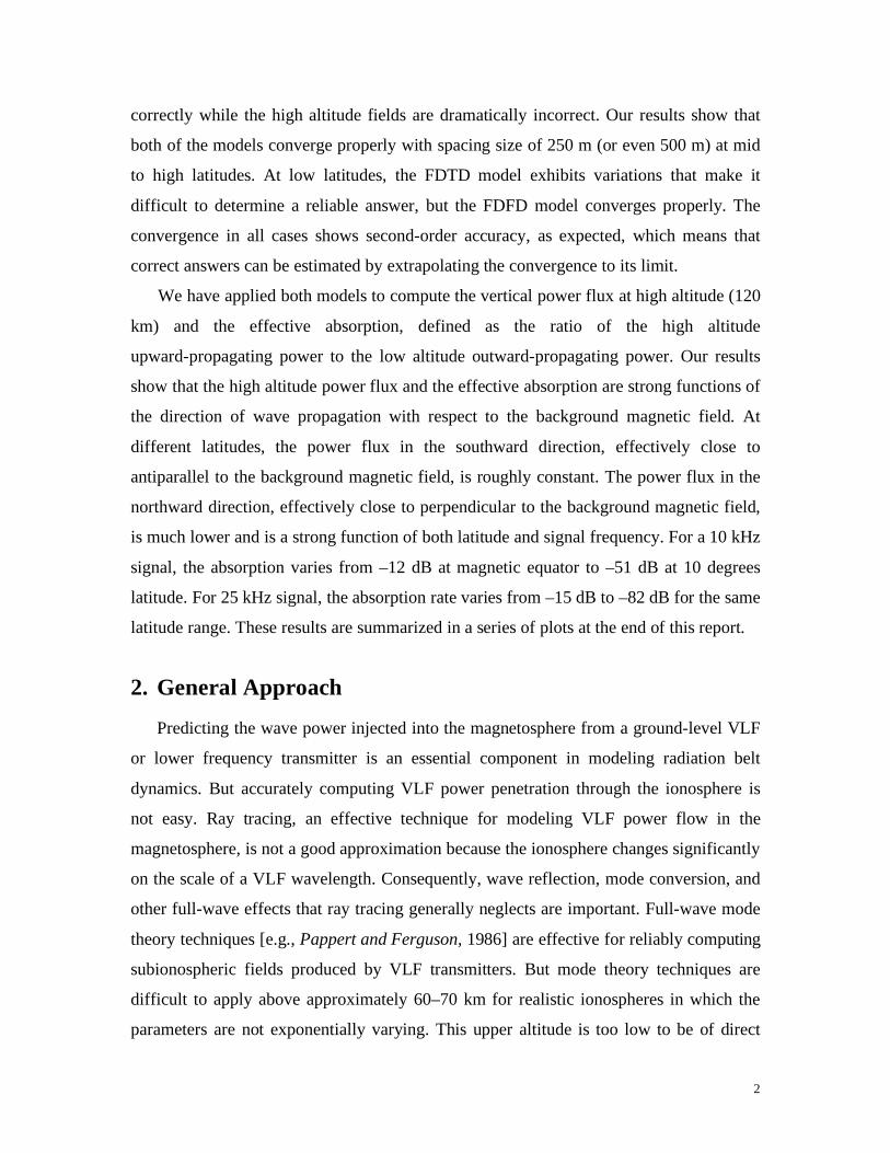
coefficient matrix. Then it solves the following equation to obtain all field components,
[ ] [ ] [ ] [ ] [ ] [ ]1M F J or F M J!
" = = " (7)
where [F] is the vector of all the time-static fields in the computation domain, [J] is the
current source vector, and [M] is the coefficient matrix derived from the governing
equations. Thus in the FDFD system, the main task is effectively invert the large sparse
matrix [M]. One possible method is to use iterative solvers to solve the linear equations.
However, because the [M] matrix is complex and ill-conditioned, none of the existing
iterative solvers are guaranteed to converge and we were not able to obtain reliable
results. Instead we use the sparse direct solver in Matlab, which is optimized for
Gaussian-elimination method, to solve the problem. Figure 5 shows all the 6 field
components computed using the FDFD model. The settings are the same as the FDTD
simulation results previously shown in Figure 4. The simulation results from the FDFD

11
code (Figure 5) agree very well with that from the FDTD simulation (Figure 4). This
indicates the correctness of both methods.
Figure 5. FDFD simulation results of all the 6 field components caused by a short dipole with unit current. The transmitting frequency is 10 kHz and the Earth magnetic field is vertical.
Figure 6. Schematic of computation domain in the segmented approach
The most challenging part of the FDFD code is to compute the inverse of the
coefficient matrix. For a large computation domain or fine grid spacing, the coefficient
matrix is large and requires substantial computer memory. To obtain a more efficient

12
algorithm, we applied a segmented approach described by Chevalier et al. [2006] and
Taflove and Hagness [2000]. To apply this method, we divide the entire computation
domain into smaller segments, as shown in Figure 6. The computation of the fields in the
first segment proceeds identically as for a single segment code. After computing all field
components at all the grid points, the fields along a vertical line close to the edge of the
first segment at r1 are used as the source fields in the second segment. In the second
segment, the location r1 is the scattered field/total field boundary, at which the condition
Es + Ei = Et (8)
is satisfied. In the above, Es is the scattered field; Et is the total field; and Ei is the
incident field. The fields is from the previous segment are used as the incident fields in
the current segment. The field components in the second segment computed at r2 are
again used as the incident in the next segment, and the process continues until the
solution for the entire computation domain is computed. In this way, we reduce the
coefficient matrix size by a factor of N by splitting one entire computation domain into N
segments.
One assumption implicit in this approach is that the reflections from later segments
are small enough to be negligible. To validate this assumption, we compare the
simulation results from multi-segmented approach with that from a single domain. Figure
7 below demonstrates the correct implementation of the segmented approach in our code.
The top two panels show the vertical electric field in two adjacent segments caused by a
20 kHz transmission signal. The bottom panels show the same fields computed using 5
segments (left) and using a single segment (right). The field distributions are essentially
identical, which indicate the segmented approach can successfully approximate a single
computation domain.

13
Figure 7. Top left and right: The vertical electric field distribution from a 20 kHz high latitude transmitter in two adjacent segments using the segmented approach. Bottom left and right: Comparison of the fields computed using 5 segments (left) and one segment (right).
The segmented approach enables direct matrix solvers to be used on each segment,
which dramatically increases the speed of the code compared to one based on iterative
solvers. Since only a single frequency is computed instead of time domain signals, the
FDFD code is much faster to run than the broadband FDTD code. Table 2 below
compares the execution times for FDTD and FDFD simulations of VLF penetration from
the NPM station over a 120 km (vertical) by 1000 km (horizontal) domain. These tests

14
were run on an Intel Pentium 4 3.0 GHz processor machine. The FDFD code is about 30
to 40 times faster the FDTD code.
Table 2. Computation times for FDTD and FDTD on Matlab platform Stepsize (m) FDTD (hr) FDFD (hr) 1000 6.6 0.08 500 38 0.9 250 >200 (estimated) 4.86
4. Model Validation
Because our ultimate aim is to simulate absolute field magnitudes, validation of the
accuracy of this code is critical. Below we describe our efforts to validate the accuracy
of this code in three separate ways.
4.1 FDTD comparison with LWPC
For precisely validating the numerical correctness of the FDTD calculations, we
compare its results with predictions from the well-validated LWPC mode theory
propagation code. The results of a comparison with LWPC are in Figure 8 below,
which shows the single frequency (25.2 kHz) vertical electric field amplitude
distributions with range under identical ionospheric conditions. The two plots show two
different propagation directions relative to the horizontal component of Earth’s magnetic
field. In both cases, the quantitative agreement between our FDTD predictions and the
LWPC calculations is extremely good all the way to 3000 km range. It should be noted
that these comparisons are not absolutely calibrated because of the challenges in
comparing source amplitudes between the models. We are working towards absolutely
calibrated model comparisons. Regardless, it is clear that the FDTD code is delivering
reliable and correct low altitude field predictions.

15
Figure 8. Comparisons of LWPC and FDTD predictions of low altitude 25.2 kHz vertical electric fields as a function of range from the transmitter. Results for two distinct propagation directions relative to Earth’s magnetic field are presented, both of which yield excellent agreement. Based on the three validations made above to both experimental data and LWPC model, we can conclude that the FDTD is capable to produce reliable results.
4.2 FDTD Comparison with High Altitude Rocket Data
We validate the FDTD model by comparing with the measurements from the 1963
Aerobee set of rocket experiments, which launched one daytime and one nighttime rocket
that measured calibrated VLF E and B fields up to 200 km at a range of roughly 200 km
16
from the NSS transmitter (22.3 kHz, 100 kW at the time). Here we report results of a
comparison between simulations with our code and measurements.
Figure 9. The rocket trajectory for the daytime rocket and the flight geometry for both rockets.
Figure 10. Electron density profiles, (left) daytime and (right) nighttime
Figure 9 shows the rocket trajectory for the daytime rocket and the flight geometry
for both rockets relative to Earth’s magnetic field and the NSS transmitter. Figure 10
shows the measured electron density profiles during the daytime and nighttime launches.
Most of the key input parameters for the FDTD codes are obtained from the information
in these sets of plots.

17
Figure 11. Comparison of measured and simulated horizontal magnetic field from the daytime rocket. Simulations were run with a 300 m grid size.
Figure 11 compares the measured and simulated horizontal magnetic fields during the
daytime rocket ascent. The dB scale is relative to 1 nT. The measured fields were
reported as maximum and minimum values of the polarization ellipse, and these were
also computed from the simulation for comparison. The agreement for the maximum
fields is extremely good from low altitudes all the way to above 100 km where the
electron density exceeds 5x10⁴ per cc. The agreement ceases abruptly above this altitude,
where we know the 300 m grid size is no longer sufficient to resolve the 22.3 kHz
wavelength. But below this altitude, the agreement is within a few dB. Moreover, the
simulation captures almost perfectly the 85 km altitude where the field switches from
mostly linearly polarized (max>>min) to circularly polarized (max=min). The agreement
for the minimum field is less good, but this field is much smaller than the maximum and
we suspect that the measurements may not be reliable for these small fields.

18
Figure 12. Comparison of measured and simulated horizontal magnetic field from the nighttime rocket. Simulations were run with a 300 m grid size.
Figure 12 shows the same comparison but for the nighttime rocket. Here the
agreement is still good at low altitudes (within a few dB) but the field change at high
altitudes does not match. The simulation predicts a 10 dB drop in the field strength
between 70 and 80 km altitude, while the measurements show a smaller 5 dB drop
between 80 and 90 km. We suspect this difference is due to uncertainties in the electron
density measurements between 60 and 80 km altitude. Here the densities are small
enough that the measurements appear potentially unreliable (note the single measurement
from 60 to 80 km altitude), but these altitudes are also very important in controlling the
absorption of the upgoing VLF energy. We suspect that the density is smaller in this
altitude range than the measurements indicate. Lower densities would be completely
consistent with other reported measurements of nighttime D region electron densities
(see, for example, Cheng et al., 2006). Additional simulations (not shown) confirm that
grid size, magnetic dip angle, and electron density smoothing do not have a major impact
on the simulated fields.
19
To summarize, the daytime agreement between the main B field components is
extremely good (within 2 dB) even to high altitudes where the electron density
approaches 105 per cc. The nighttime agreement, although less good, is not bad and many
specific features in the fields are reproduced extremely well. We suspect that the
measured electron densities between 60 and 80 may not be reliable, as they seem large
compared to other reported nighttime D region measurements. This may explain the
discrepancy. Overall, the agreement between measured and simulated fields is very good
considering the uncertainties involved in resurrecting 40 year old measurements from a
written report. We consider this strong experimental validation of the FDTD code.
4.3 FDTD Convergence Test
As reported above, our FDTD model provide reliable results based on several
validation experiments. However, choosing the right grid size is critical to obtaining
reliable results. In general, finer spacing always produces more accurate results. At the
cost of dramatically increase the computation time. To quantify the connection between
grid spacing, geomagnetic latitude, and simulation accuracy, we ran a series of
simulations for different magnetic latitudes. Thus in the following discussion and
simulations, “latitude” in our text is referred to magnetic latitude expect the places where
geographic latitude is explicitly stated. Finite difference simulations are guaranteed to
eventually converge to the correct answer as this grid spacing is reduced, but it is not
always easy to know what grid spacing is required to maintain errors below a specified
level. We have found that, for a given uniform grid spacing, the low altitude fields can be
computed correctly while the high altitude fields are dramatically incorrect. At mid to
high latitudes, 500 m grid spacing results is fairly accurate to obtain high altitude fields in
the 10–25 kHz band. But at low latitudes, 250 m and smaller grid spacing is required to
achieve the same accuracy. The convergence in all cases shows second-order accuracy,
which is as expected.
Here we show the FDTD model convergence at different locations within 200 km of
the VLF transmitter (short range is required for the simulations to be manageable for fine
grids) at latitudes from the geomagnetic pole to the equator. The radiation source is

20
assumed as a short monopole and the transmitting frequencies are at 10 kHz and 25 kHz.
The earth magnetic field is computed from a simple dipole model
3
03
0
2 2
1
2* *(1/ )*sin( )
*(1/ )*cos( )
90 tan (| | / | )
r
r
r
B B rB B r
B B B
B B
!
!
!
"
"
# $
= $
=
= +
= $
(9)
where B0 = 3.12e-5 Tesla is the magnetic field magnitude at the equator, λ is the magnetic
latitude, and α is the codip angle.
At each latitude and frequency, we ran the simulations with grid sizes of 1000 m, 500
m and 250 m. Simulation results from the above spacing sizes and the second order
convergence allow us to estimate the true field components using
500 500
250 250 250 250 500
500 250
( ) / 34*
F F EF F E F F F FE E
= +
= + ! = + "
=
(10)
where F is the true field, Fn is the simulation result with grid size of n, and En is the error
for spacing grid of n.
The figures below shows the convergence of one component of electric field caused
by unit current. The results are essentially identical for all E and H components. We
also plot the error relative to the estimated solution for grid sizes of 1000 m, 500 m, and
250 m respectively. Figure 13 shows the FDTD simulation results at Mlat = 80 degrees
for transmitting frequency of 10 kHz. The top panels show the electric field component
(Eφ) at high (120 km) and low (60 km) altitudes. The bottom panels show the error in
percentage relative to the best estimate. At both altitudes, the fields are almost invariant
to grid spacing, indicating that the solution has converged even at 1 km spacing and
consequently that these results are numerically correct.

21
Figure 13. FDTD convergence for f = 10 kHz, Mlat = 80 degrees.
Figure 14. FDTD convergence for f = 10 kHz, Mlat = 50 degrees.
Figure 14 shows the same quantities as Figure 13 but at a magnetic latitude of 50
degree. At distance within a few tens kilometers from the transmitter, the FDTD

22
simulation results have an artificial effect at higher altitudes (>100 km) caused by the
magnetic field in the direction of propagation. However, this artificial effect does not
affect the computations at other locations and thus is ignored in the Figure 14 (region less
than 20 km in left panels). At low altitude (60 km), fields are still invariant for the three
different grid sizes. However, at high altitude (120 km), the result of 1000 m spacing
deviates from the best estimate with an average error about 20%. The results from
spacing of 500 m and 250 m are still fairly close to the best estimate with an average
error of 6% and 1.5% respectively. Thus the three error rates from 250 m, 500 m and
1000m spacing contrast a ratio of 1:4:13. This clearly shows the second order
convergence introduced earlier especially for fine grids, i.e. 500 m and 250 m spacings.
This example also indicates that high altitude fields require finer grid spacing as the
latitude decrease.
Figure 15. FDTD convergence for f = 10 kHz, Mlat = 30 degrees.
Figure 15 shows the high altitude and low altitude fields at 30 degrees latitude. At
low altitude (60 km), solutions from the three grid sizes still yield the same results. At
high altitudes, solutions from different grid sizes deviate as expected. The relative errors
increase to 65%, 20% and 5% for grid sizes of 1000 m, 500 m, and 250 m. Similar to the

23
simulation results at 50 degree latitude, the three error rates contrast a ratio of 1:4:13,
which again indicates the second order convergence.
Figure 16 shows the relative error or results from 250 m spacing to the best estimate
at different latitudes. For low altitude fields, the FDTD always converges to the answer
with an error less than 1%. However, the high altitude field convergence significantly
affected by the latitude. The error increases from less than 0.1% to more than 10% for
latitudes near the pole to the 20 degrees. For latitudes below 20 degree, the FDTD
simulations of high altitude fields do not converge well and we are not able to obtain
reliable results. For latitudes lower than 20 degrees we use the FDFD model described
in the next section.
Figure 16. Average error of results from 250 m grid size to the best estimate at different latitudes for transmission frequency of 10 kHz. The blue stars represent errors at high altitude and the red stars represent the errors at low altitude.
To study the dependence of convergence on transmission frequency, we also
compare the simulation results with different grid spacing for 25 kHz signal. Figures
17–19 show the same quantities as Figures 13–15 but for transmission frequency of 25
kHz. Figure 17 shows the field convergence of a 25 kHz signal at 80 degree latitude. In
both high and low altitudes, the solution from 1000 m spacing starts to deviate. However,
solutions from 500 m and 250 m are almost identical. This indicates higher frequency
requires a finer grid as expected.

24
Figure 17. FDTD convergence for f = 25 kHz, Mlat = 80 degrees.
Figure 18. FDTD convergence for f = 25 kHz, Mlat = 50 degrees.

25
Figure 19. FDTD convergence for f = 25 kHz, Mlat = 30 degrees.
Figure 18 and Figure 19 show the field convergence at mid (50 degrees) and low (30
degrees) latitudes for a transmission frequency of 25 kHz. At mid latitude, the field high
altitude field components still converge toward the solution although the error at a given
grid size is larger than for high latitudes. All the three solutions have the same shape and
the relative error of result from 250 m spacing is within 7%. At low altitudes, the fields
from different simulations are still fairly close to the best estimate, again indicating that
the low altitude convergence is largely independent of background magnetic field. The
low latitude results in Figure 19 further confirm these general findings. Figure 20
summarizes the relative error for a 25 kHz transmission signal. The pattern is similar to
the 10 kHz signal, with a small and nearly latitude-independent low altitude relative error,
and a latitude-dependent high altitude relative error. Note that below 30 degrees latitude,
the high altitude FDTD simulated fields does not converge well and appears to be
unreliable.

26
Figure 20. Average error of simulation results from 250 m spacing to the best estimate at the different latitudes for transmission frequency of 25 kHz. The blue stars represent errors at high altitudes and the red stars represent the errors at low altitudes.
In summary, the low altitude fields converge to an accurate answer with 500 m or
even 1000 m grid size independent of latitude. The high altitude field convergence is
strongly dependent on the background magnetic field. For high latitudes above 70
degrees, a grid size of 500 m or even 1000 m is fine enough to compute the high altitude
fields with small errors of several percent. For mid latitudes of 40 to 60 degrees, a smaller
grid size of 250 m still yields accurate simulations with an uncertainty of a few percent.
At low latitudes of 20 to 30 degree, the relative error of 250 m grid size increases to a few
tens of percent. Below 20 to 30 degrees latitude, the FDTD results do not converge well
and are unreliable. This low latitude problem is solved with a different simulation
technique as described in the following section.
4.4 FDFD Comparison to FDTD
In Section 3, we demonstrated qualitatively good agreement between the FDTD
simulation and FDFD simulation results. We now investigate the convergence of the

27
FDFD solution with different grid sizes to understand what parameters are needed to
yield a correct solution. We do this by comparing the FDFD solutions with the known
correct FDTD solutions, which has been validated and tested in several different ways as
described above. We have run a series of simulations with the same settings as the FDTD
code introduced in the previous section. Similar to the FDTD code, the FDFD code also
exhibits second order convergence, and we again extrapolate to the correct value with
equation (10).
Our simulations show that the FDFD model contains the same physics and provides
the same results as the FDTD model. The convergence of FDFD code is also generally
similar to the FDTD code. The low altitude field convergence is almost independent of
latitude and frequency, while the high altitude field convergence depends on the latitude.
As the latitude decrease, the relative difference between the two smallest grid size
simulations increases from less than 1% to several tens of percent. In contrast to the
FDTD simulation, which does not always converge well below 20 degrees latitude, the
FDFD simulations at all latitudes are always stable.
Figure 21 shows the FDFD convergence for 10 kHz signal at 80 degree latitude.
The top panels show one component of electric field at high altitude (120 km) and low
altitude (60 km). Blue, red and black lines represent the FDFD simulation results from
grid spacing of 1000 m, 500 m, and 250 m respectively. The green line and yellow lines
represent the best estimates from FDFD and FDTD simulation results based on the
second order convergence. If we consider the best extrapolated value from the FDTD
simulation as the true answer, the relative error of the FDFD simulation result with grid
spacing of 250 m and the best extrapolation are shown in the bottom panels. In this
example, the average error between the two best estimates is within a few percent in both
high and low altitude fields. This confirms the correctness of our FDFD model.

28
Figure 21. FDFD convergence for f = 10 kHz, Mlat =80 degrees.
Figure 22. FDFD convergence for f = 10 kHz, Mlat = 50 degrees.

29
Figure 22 shows the same quantities as Figure 21 but at 50 degrees magnetic
latitude. In this example, the difference between the two codes at low altitude is still just
a few percent and comparable to that at higher latitude. However, comparing to the
simulation result at 80 degrees latitude, the relative error of the high altitude fields
increases due to the decrease of latitude. The discrepancy between the FDTD and FDFD
estimates is about 10 percent. This relatively small factor represents the uncertainty in the
absolute field and power magnitudes in our simulations at mid latitudes.
Figure 23. FDFD convergence for f = 10 kHz, Mlat = 30 degrees.
Figure 23 shows the same field comparison at low latitude. Although the fields at
low altitude still agree within a few percent, at high altitudes, the relative error between
the two codes increases to 50%, with the FDFD code giving the smaller value. Although
the relative error between FDFD and FDTD increases at low altitudes, the three FDTD
simulation results from different grid spacing still have the same shape as the FDTD
simulation result.

30
Figure 24. The relative error between FDFD and FDTD best estimates for high and low altitude fields with a signal frequency of 10 kHz.
Figure 24 summarizes the relative discrepancy between the FDTD and FDFD best
estimates for a 10 kHz signal. At low altitudes, the two models always agree well within
a few percent at all latitudes. As the latitude decreases, the relative error of the high
altitude fields increases up to 60% at latitude of 20 degrees. Below 20 degrees, the FDTD
simulation does not reliably converge. However, the FDFD simulation always
converges toward to the right answer even at low altitudes. This makes the FDFD code a
complimentary tool to the FDTD model at low latitudes although the absolute uncertainty
becomes larger at low latitudes. Thus for transmission frequency of 10 kHz, we use the
FDFD model to compute the field and radiated power for magnetic latitude less than 20
degrees. At mid to low latitudes, our simulation results show that the best estimate from
FDFD model is consistently smaller than that from FDTD by a factor of 2 at 30 degrees
latitude and a factor of 3 at 20 degrees. When the FDTD code converges, it does so more
quickly and reliably than the FDFD code. For that reason, we feel that the converged
FDTD result is more reliable when it exists. Thus the low latitude FDFD results should
be considered a lower bound to the correct answer and may underestimate the true fields
by a factor of 2 to 3 at latitudes below 30 degrees.

31
We also examine the FDFD convergence for a transmission frequency of 25 kHz
signal. Figures 25–27 show the convergence of 25 kHz signal at latitudes of 80, 50 and
30 degrees in the same format as above.
Figure 25. FDFD convergence of f= 25 kHz, Mlat = 80 degrees.
Figure 25 shows the FDFD convergence of 25 kHz signal at 80 degrees latitude.
Fields at both high and low altitudes converge to the same result as the FDTD code. At
high altitude (120 km), the relative error between the FDFD and FDTD estimates is
within a few percent and at low altitude (60 km), the relative error is below 10%. Note
that the largest low altitude error occurs near field nulls meaning that the absolute error is
still relatively small.

32
Figure 26. FDFD convergence of f = 25 kHz, Mlat = 50 degrees.
Figure 27. FDFD convergence for f = 25 kHz, Mlat = 30 degrees.

33
Figure 26 and 27 show the convergence of 25 kHz signal at 50 degree and 30 degree
latitude. The agreement between FDFD and FDTD is still good at low latitudes, although
the relative difference still increases as the latitude decreases.
Figure 28. Relative difference between FDFD and FDTD results for low and high altitudes simulations for a 25 kHz signal.
Figure 28 summarizes the average relative error between FDTD and FDTD estimates
as a function of latitude for a 25 kHz source. As for the 10 kHz source, the error at low
altitude is essentially independent of latitude and small. The high altitude error
increases with decreasing latitude but never becomes so large as to invalidate the results.
Based on the above analysis, we conclude that the FDFD model basically contains the
same physics as the FDTD model. It also provides the same results as the FDTD model.
Thus the FDFD model is fast and reliable for single frequency simulations of ionospheric
VLF power penetration.

34
5. Results
In this section, we summarize our main findings. First we present detailed simulations
of the upward power flux at high altitude (120 km) specifically for the NML VLF
transmitter. Then we summarize general results for high altitude vertical power flux for
10 kHz and 25 kHz transmitted signal as a function of magnetic latitude. This summary is
presented in several forms.
5.1 Upward VLF Power from the NML Transmitter
To demonstrate the full model capability, Figure 29 shows the east-west spatial
distribution of all 6 electromagnetic field components in cylindrical coordinates
generated by a 25.2 kHz VLF transmitter with 233 kW radiated power at the location of
NML (Geo Lat = 46.36° N, Geo Lon = 98.29° W, codip = 17.2° ). The horizontal scale in
the figure is significantly compressed and the magnetic field components are normalized
by the speed of light to convert them to units of V/m, like the electric fields. Several
qualitatively correct features are immediately visible. The fields abruptly change from a
variety of wave normal angles below 90 km altitude to almost entirely upward
propagating above 90 km, where the fields can legitimately be considered to be
propagating in the whistler mode. The strongest field components at low altitudes are
Ez and Bφ, the primary components produced by a vertical electric dipole source. Other
components generated only through the anisotropy of the ionosphere are present at
smaller amplitudes. In contrast, at high altitudes the horizontal components Er, Eφ, Br,
and Bφ are the largest. Moreover, Er and Eφ are almost equal in magnitude, as are Br and
Bφ, reflecting the nearly circular polarization of the high altitude fields. Lastly, clear
east-west anisotropy is visible in the fields, which again is expected.

35
Figure 29. The spatial distribution in an east-west plane for all 6 electromagnetic field components in cylindrical coordinates produced by a 25.2 kHz transmitter at the location of NML. A fully inhomogeneous background magnetic field is included which is responsible for the visible east-west anisotropy.
As has been noted before, different ways of validation make it clear that the correct
physics are being modeled. We also need to confirm that the results are quantitatively
correct by evaluating the convergence of the simulations with changing grid size. This
power convergence is demonstrated in Figure 30, which shows the east-west slice of
upward propagating power at 120 km altitude from a 233 kW, 25.2 kHz transmitter at the
location of NML as a function of spatial grid size in the simulation. The anisotropy
produced by Earth’s magnetic field is again clear. It is also clear that although a 1000 m
grid size underpredicts the upward power, 500 m and 250 m give almost the same
answer. This shows that the 250 m calculation has essentially converged to the correct
answer given the physics in the model. By using the 250 m spacing size, we show in
Figure 31 the vertical power flux at 120 km latitude for wave power in 8 horizontal
directions from the NML transmitter. This gives a complete picture of the high altitude
upward power flow over a 1000 km diameter circle around the transmitter location.

36
Figure 30. Convergence analysis of the upward VLF power at 120 km altitude from the NML transmitter. The computation with 1000 m grid size underpredicts the power, but the 500 and 250 m computations are almost identical, indicating that this is the converged and therefore correct answer.
It should be noted that although it is not shown here, these predictions are in excellent
quantitative agreement with those from a completely different numerical model [Lehtinen
and Inan, 2008]. Interestingly, these predictions are also in adequate agreement with the
simplified empirical model predictions that lead to a significant overprediction of the
high altitude fields measured by satellites [Starks et al., 2008]. Consequently it appears
as though some process is scattering or absorbing a great deal of VLF wave power
between 100 and 700 km altitude. As a step towards understanding what processes might
be responsible for this discrepancy, we carefully examined the distribution of the k vector
angle at high altitudes from the NML transmitter. A summary of these calculations is
shown in Figure 32. It is well understood that the high refractive index of the whistler
mode results in wave vectors that are largely vertical at high altitudes. However, it must
also be realized that much of the low altitude wave power is grazingly incident on the
lower edge of the ionosphere and thus the horizontal component of the wave vector can
be quite large. Figure 32 highlights this by showing that the wave vector at 120 km
altitude in most locations except very close to the transmitter (<50 km) is typically 20 to
30 degrees away from vertical, with the horizontal component pointing away from the
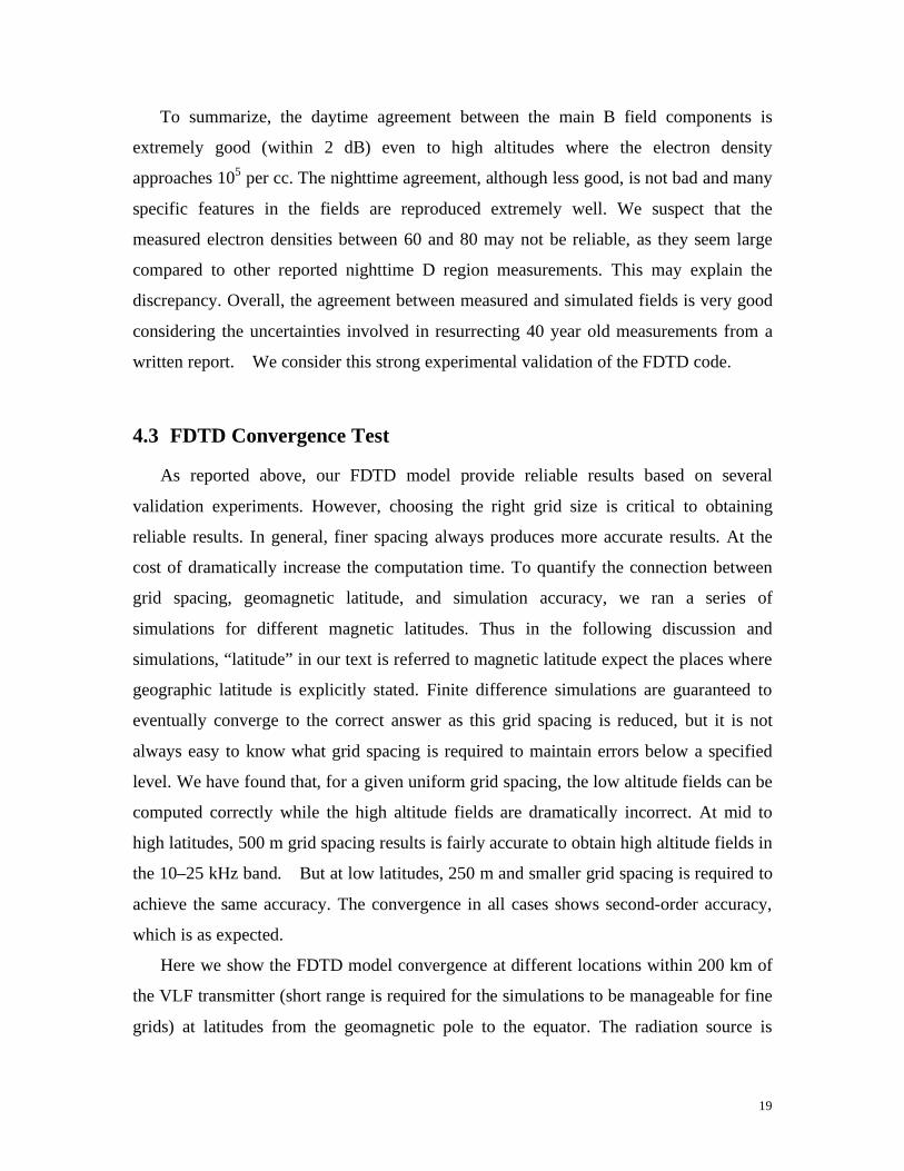
37
transmitter location. The degree to which this might contribute to additional power
spreading at high altitudes could be confirmed with ray tracing. It may be negligible,
but it may not.
Figure 31. A full geographic distribution of the upward power flux at 120 km altitude from the NML transmitter.

38
Figure 32. Calculation of the spatial distribution of the wave vector direction at 120 km altitude from the NML transmitter.
5.2 High Altitude VLF Power Versus Latitude
We now compute and summarize the vertical power flux at high altitude (120 km) as
a function of magnetic latitude to better understand the latitude dependence of how VLF
power escapes the ionosphere. In all the simulations, the source is modeled as a 1 km
vertical electric monopole at the ground with a total radiated power of 1 kW. A 2
parameter exponential nighttime electron density profile (h’ = 85 km and β = 0.5) is used
to simulate the environment, where h’ controls the altitude of the profile and β controls
the sharpness of the ionospheric transition [Cummer et al., 1998]. The computational
domain is 500 km (distance) by 120 km (altitude). At each latitude, waves are injected in
8 horizontal directions azimuthally spaced every 45 degrees. We compute the vertical
power density at 120 km altitude as well as the ratio between high altitude upward power
flux and low altitude radial power flux to obtain what we call an “effective absorption
rate”, although it should be noted that this ratio of high altitude upward power flux to low

39
altitude outward power flux does not represent an actual absorption. In all of these
computations, we have scaled the simulation results to the best estimates based on the
convergence test in the previous section.
Figure 33 shows the results for a transmission frequency of 10 kHz at high, mid, and
low latitudes. The left panels show the vertical power density per kW transmitted at 120
km altitude. The right panels show the ratio between the vertical power flux and 120 km
altitude and the horizontal power flux at ground. At high latitudes, the power flux
densities at all directions are almost identical because the background magnetic field is
almost completely vertical. As the latitude decreases, the power density becomes
increasingly affected by the wave propagation direction. The power density to the north
of the transmitter is smaller than the power density to the south because the power flow is
more parallel to the background magnetic field to the south. This strong anisotropy is
seen in the effective absorption plot.
To further study this anisotropy, we plot the total power density magnitude and
direction in the entire computational domain for two propagation paths of 45 degree
(north east) and 225 degree (south west) at 30 degrees latitude in Figure 34. Below 90
km altitude, the power flux is almost in horizontal direction for distances a few hundred
kilometers away from the transmitter. However, there are some differences in the low
altitude power flow patterns. The power flow in the 225 degree direction contains more
upward flow than that in 45 degree direction, which indicates less reflection and allows
more power penetration into the ionosphere. For altitudes above 100 km altitudes, the
power flux is close to the direction of the background magnetic field for both propagation
paths, as expected from whistler mode refractive index surface. Thus in the transition
region of ~ 80 – 100 km altitude, the power flow in the 45 degree case actually bends
backwards away from the transmitter, while the power flow in the 225 degree case
changes direction far less. The strong azimuthal dependence of upward power
transmission through the ionosphere is expected and seen in the simulations.

40
Figure 33. Vertical power flux and power absorption at 120 km altitudes for 80, 50 and 30 degree latitudes. The transmission signal is 10 kHz. The left panels show the vertical power flux. The right panels show the ratio between the vertical power flux at 120 km altitude and the horizontal power flux at ground.

41
Figure 34. Total power flux in a computation domain of 500 km x 120 km for propagation path of 45 degree (north east) and 225 degree (south west). The color intensity and the arrow on each plot represent the magnitude and direction of power flux.
42
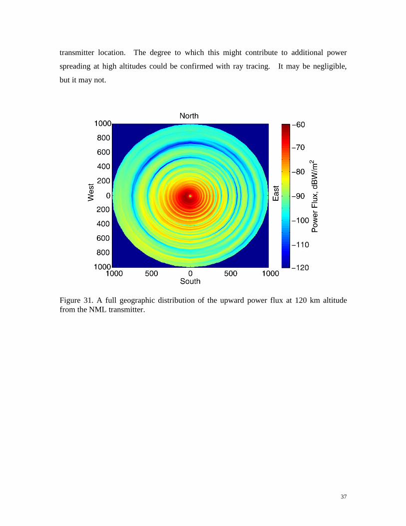
Figure 35. Vertical Power Flux and absorption rate at 25 kHz. Left panels show the vertical power flux at three latitudes. Right panels show the ratio between high altitude vertical power flux and low altitude horizontal power flux.
Figure 35 shows the same quantities as Figure 33 but for a transmission frequency of
25 kHz. The results are similar to that from 10 kHz signal except that the dependence of
power flux on wave direction is even stronger at low latitude.

43
We now summarize the high altitude vertical power flux and effective absorption rate
for 10 kHz and 25 kHz signal. To do this we need to reduce the entire radially varying
upward power flux curve to a single number. The calculations above show that almost
all of the upward power flux is transmitted through the ionosphere between 50 and 200
km radial distance from the transmitter, and we thus average the power densities over this
range. The absorption rate is simply represented by the ratio of the average upward power
over the average outward power.
Figure 36. Average upward power flux per kW transmitted at 120 km altitude. Top: f = 10 kHz. Bottom: f = 25 kHz.
Figure 36 shows the average power density per kW transmitted at high altitude (120
km). The power flux densities in the 8 different azimuthal directions are represented by
different symbols. At high latitudes, all the directions exhibit essentially the same power
density because the horizontal component of the background magnetic field is small. As
the latitude decreases, the power density shows significant differences in different
propagation directions. For waves traveling south (and up), which puts them close to
anti-parallel to the background magnetic field, the average upward power flux is close to
a constant –90 dBW/m2 per kW transmitted. Even though this power flux at 120 km

44
altitude is close to uniform with latitude, the fraction of power that makes it even higher
into the ionosphere will have a strong dependence on latitude.
For the waves traveling north (and up), which requires them to move power across
the background magnetic field, the power density dramatically decreases as the latitude
decrease. This is expected because in general whistler mode wave power cannot
propagate at large angles with respect to the background magnetic field. In our results,
this power density decreases from –88 dBw/m2 to –132 dBw/m2 for 10 kHz and from –91
dBw/m2 to –163 dBw/m2 for 25 kHz.
Note that the results in Figure 36 for 10 kHz and 10 degrees latitude and 25 kHz and
10 and 20 degrees latitude were computed with the FDFD code while the other results
were computed with the FDTD code. As discussed above in Section 4.4, the FDFD
results may underestimate the true fields by a factor of 2 or 3, resulting in a power level
underestimate of as much as 6 to 10 dB. Since the low latitude absorption is already very
high for most azimuth angles, this uncertainty does not impact the practical consequences
of our results.
To compare the different effects caused by electron density profiles, a daytime
ionosphere profile (h’ = 75 km, β = 0.4) is also used to simulate the upward power flux at
50 degrees magnetic latitude. The high altitude power with daytime profile is much less
than that from the nighttime profile due to more absorption caused by higher number of
charged particles. The higher number density of electrons and ions also result in
essentially no anisotropy in the different propagation direction for a daytime ionosphere.
45
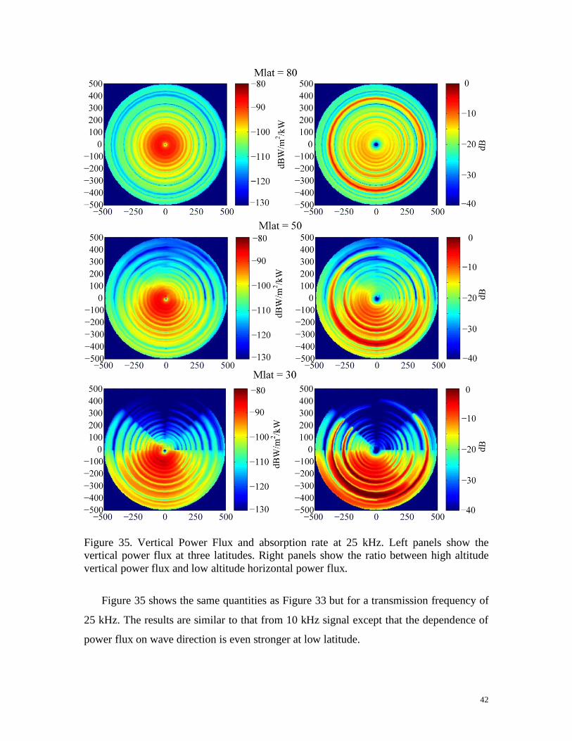
Figure 37. Average ratio of high altitude average upward power density to average outward power density at ground. Top: f = 10 kHz. Bottom: f = 25 kHz.
Summarizing the results in a slightly different form, Figure 37 shows ratio of high
altitude power flux to low altitude power flux. As mentioned earlier we refer to this ratio
as an effective absorption rate, and it is computed from spatially averaged values from 50
to 200 km radius from the transmitter. We compute it here because prior work in this
area used a simplified low altitude VLF absorption model with simulations of upward
propagating whistler mode energy to estimate high altitude power flux. We remind the
reader that this approach, although it delivered not unreasonable quantitative predictions,
misapplies the whistler mode simulations of Helliwell [1965]. There is a significant
difference between low altitude outward VLF power flux and a whistler mode wave
normally incident (i.e., upward propagating) on the lower ionosphere. This effective
absorption depends on latitude in the same way as the average power density because the
outward power density at the ground level is almost invariant at different latitudes. For
a 10 kHz signal, the effective absorption rate is about –12 dB at magnetic pole. This
value is about 10 dB higher than the upward whistler wave attenuation reported by
Helliwell [1965]. As the latitude decreases, the maximum absorption occurs when the

46
wave power propagates close to the north direction, as expected. This maximum 10 kHz
effective absorption increases to –56 dB at 10 degrees latitude. For a 25 kHz signal, the
maximum (to the north) effective absorption varies from –15 dB to –87 dB from
magnetic pole to 10 degrees latitude.
Figure 37 also reproduces for comparison the upward-propagating whistler absorption
curves from Helliwell [1965]. Despite the fact that they represent different physical
quantities, the numbers are quantitatively consistent, particularly at mid latitudes, which
explains why the scaling approach based on this “Helliwell curve” has generally yielded
good results despite being a not quite appropriate application of those simulations.
It is interesting to note that south of the transmitter, the effective absorption is
dramatically lower, with values generally between –10 dB and –20 dB for all magnetic
latitudes. This occurs for the reason mentioned above, namely that wave power in this
direction propagates generally along the background magnetic field direction, even at
fairly low latitudes, and thus is able to escape the lower ionosphere fairly efficiently.
However, it should again be emphasized that this does not mean that this energy is able to
travel to higher altitudes. At low latitudes the relatively horizontal background
magnetic field ensures the wave power is confined to relatively low altitudes and thus
would not participate in radiation belt dynamics. Ray tracing simulations of this
escaping wave power should confirm this.
For completeness we also compute the midlatitude daytime effective absorption. As
in the figure, these absorptions are –48 dB and –38 dB for 10 kHz and 25 kHz signals,
respectively. That the effective absorption is higher at low frequencies is a bit of a
surprise. This could be caused by non-convergence of the 25 kHz daytime simulations
with the 250 m grid size used in these simulations, which in turn would be caused by the
shorter whistler mode wavelengths resulting from higher daytime electron densities.
Nevertheless it is clear that daytime VLF wave transmission through the lower
ionosphere is almost certainly too weak to play a role in radiation belt particle loss.

47
REFERENCES
Budden, K. G., The propagation of Radio Waves, Cambridge Univ. Press, New York, 1985.
Cheng, Z., S. A. Cummer, D. N. Baker, and S. G. Kanekal, Nighttime D region electron density profiles and variabilities inferred from broadband measurements using VLF radio emissions from lightning, J. Geophys. Res., 111, A05302, doi:10.1029/2005JA011308, 2006
Chevalier, M. W. and U. S. Inan, A technique for efficiently modeling long-path propagation for use in both FDFD and FDTD, IEEE Antennas and Wireless Propagation Letters, 5, 525-528, 2006
Cummer, S. A, U. S. Inan and T. F. Bell, Ionospheric D region remote sensing using VLF radio atmospherics, Radio Science, 33, 1781-1792, 1998.
Cummer, S. A., Modeling electromagnetic propagation in the Earth-ionosphere waveguide, IEEE Transactions on Antennas and Propagation, 48, 1420-1429, 2000.
Cummer, S. A., A simple, nearly perfectly matched layer for general electromagnetic media, IEEE Microwave and Wireless Components Letters, 13, 128-130, 2003.
Helliwell, R. A., Whistlers and Related Ionospheric Phenomena, Stanford Univ. Press, Stanford, California, 1965.
Hu, W. and S. A. Cummer, An FDTD model for low and high altitude lightning-generated EM fields, IEEE Transactions on Antennas and Propagation, 54, 1513–1522, 2006.
Lehtinen N., G. and U. S. Inan, Radiation of ELF/VLF waves by harmonically varying currents into stratified ionosphere with application to radiation by a modulated electrojet. Journal of Geophysical Research, 113, A06301, 2008
Pappert, R. A. and J. A. Ferguson, VLF/ELF mode conversion model calculations for air to air transmission in the earth-ionosphere waveguide, Radio Science, 21, 551, 1986.
Starks, M. J., R. A. Quinn, G. P. Ginet, J. M. Albert, G. S. Sales, B. W. Reinisch and P. Song, Illumination of the plasmasphere by terrestrial very low frequency transmitters: Model validation, Journal of Geophysical Research, 113, A09320, 2008.
Taflove, A. and S. C. Hagness, Computational Electrodynamics: The Finite-Difference Time-Domain Method, Artech House, Norwood, Mass., 2000