A WORKSHOP IN EXPLORATION GEOPHYSICS OF THE SHALLOW SUBSURFACE

Dr. FRANK REVETIA Geology Department

Potsdam College of the State University of New York

Potsdam, N.Y. 13676

SEISMIC REFRACflON METHOD

Applications

W4

The seismic refraction method has many applications in shallow subsurface geologic investigations. The classic application is the detennination of depth to bedrock. The method also plays an important role in groundwater investigations since it is possible to detennine depth to water table. It is also an excellent tool in engineering and environmental studies since it makes possible the evaluation of dam sites, highways, bridges and landfill sites. Finally it is an excellent method of teaching refraction seismology principles that are used to investigate the crustal structure of the earth. Our seismic refraction survey will be used to detennine the depth to bedrock and water table on the Potsdam College campus.

Equipment

The ES-1225 exploration seismograph will be used to conduct the seismic refraction survey. The instrument is a multichannel CRT-display, printing, signal enhancement shallow exploration seismograph. It is microprocessor-based battery operated and has 12 channels. The instrument is a light and portable field unit. A portable laptop computer with an RS-232 interface will be used in the field to store the data, print seismograms of the seimic traces and analyze the time-distance graph.

The assembly of the ES-1225 system is shown in Figure 1. The geophone cable is laid out and geophones implanted firmly in the earth and connected to the cable. The battery is connected to 12 volts D.C. outlet and the sledgeharnnmer with switch is connected to start on the seismograph. A steel plate is placed firmly in the ground at an offset of 10 feet from the nearest geophone. Impacting the plate with sledgehammer when seismograph reads acquisition of data will produce a seismic record with 12 traces (Figure 2). The seismic traces may be seen on a screen and a record of them may be obtained using the print option. The data may also be entered into a portable computer so traces may be seen on a computer monitor.

255

W4

Ar r r;,.t

, aoe

Sledjen ~ mmer Handle

Biltte ry

Figure I: Assembly of the ES-1225 exploration seismograph

Seismic Refraction Method

Seismic refraction requires the generation of seismic waves into the subsurface and an instrument to detect and record the returning refracted waves. We will use an eight pound sledgehammer to generate the seismic waves and a Model ES-1225 Exploration Seismograph to record the waves. The seismograph enables us to accurately measure the travel times of the seismic waves to 12 geophones. The shotpoint and geophones are located along a line so one may plot a travel-time curve of distance versus time. The curve is used to determine velocities and calculate the depths to various layers of rock in the subsurface.

The first arrival times are measured during a refraction survey. These times represent the minimum travel time paths of the seismic waves. These minimum travel time paths are the direct waves arriving at the nearby geophones and the critically refracted waves arriving at the more distant geophones (Figure 3). The refraction method relies on the velocities of the rocks increasing with depth otherwise a critically'refracted wave will not occur. Also the length of the geophone spread must be several times the depth of the layers being investigated.

Reading the Seismograms

A typical seismic record of a seismic refraction survey is shown in Figure 2. The vertical lines are time lines with each line representing 2 milliseconds. The horizontal lives are the

256

W4

E~~~ t~U"E"ICI eM ." r5 v, OIl •• 0 • •• t r r LE' NO

2 , IS

_(CORD T1ME J l' lZ

- f- f· I z~ ..u. .f--I-F-f-~ ....-.. ./ . '", I-.

I""- r. ~. " ..(.

"e "S[C .. 24 t, , l. 15

D£LAY T 1"£ ' l. 15

... S[C 7 36 1 J

, 42 13

r-J: .. ~ t- :-

'): -~ ..... ... ""

./ - -STAC K COUt" , 42 IZ

• l' 4' 11

Il 4' I! F'U.T£.t cur It 54 Ii

1- '- }:~~ ~ --~ ... r--~-- "- :--

Figure 2: Seismic record showing 12 traces in variable area (VA) mode

traces made from the output of 12 geophones with the top trace representing the nearest geophone at 10 feet offset and the bottom trace representing the output of the furthest geophone at 120 feet distance. The numbers on the left are channel numbers, gain and trace size set for each channel. This is a variable area trace (VA) however wiggle-traces (WT) are also available. First arrival times are determined by picking the first break in the trace. The first break picks are indicated by the arrows in Figure 2. For example trace 1 has a travel time of about 11 .8 msecs while trace 12 shows a travel time of about 33 msecs. Trace 1 is the time for the seismic wave to travel 10 feet since geophone 1 is 10 feet from the shot point while trace 12 is first arrival time at a distance of 120 feet.

Seismic records may also be drawn from the data transfered to the laptop portable computer. The advantages of this method is the traces may be enhanced to help pick the first arrivals and the time scale may be increased to make more accurate time measurements. Also many seismic surveys can be conducted in a day with all the data stored in the laptop. It is also possible to do the time-distance graph with the computer using the SEISVIEW program.

Figure 4 shows two seismic records of traces produced by the laptop computer data. Figure 4a shows the traces 3 and 4 have poor first breaks. Enhancement of these traces with the hlptop computer is shown in Figure 4b where the first breaks are seen' more clearly. In Figure 5 the time scale was increased so' 1 mm equals 0.2 msec.

Analysis of seismic data

The travel times of the first arrivals may be determined from the seismic record. The first arrivals are plotted to construct a time-distance curve with the distance plotted as the X horizontal axis and the time in milliseconds plotted is the Y or vertical axis. Figure 6 shows

257

W4

u • III

c:

• E ~

7 •

" VI','

~~ ~ ~ V ~' ~O\O

{ /~ '.J~ ~ 0,0 SEISMIC •

:i 'h TRAVEL- TIME GRAPH

Based on , ArliyQJL·r-

g~ on Record and Oi.tonc. <,>0

from S ,ot Point ~,

/ D'itonee from Shot POint In ft.

,...shot InSIOnt

2

SEISMIC DETECTORS 3 4

Galvanometer "/ Tracel for

each Detector Chonnel

SEISMIC RECORD

REFRACTED TRAVEL PATHS ,

Figure 3: Travel-time graph, seismic record and wave paths of a seismic refraction survey (From Woollard 1954)

258

W4

-A, .~'. ..... ,Alb... /Mh. __________ ~_

'" ........ ." = _ rft , ,-_.- , ~'--'

- -_..-.._---'--i - . ____ - I ..... ...

i i, i -~_ : , I __ : ;,. ... -----------------...;----------.-

-- _' m '.

70 89 lOG I~HE:

Figure 4a: Seismic traces drnwn from output to laptop computer. Seismic record before enhancement of traces 3 and 4

---'"'~-'

, : I i I J _-__ -_ -----J.. ill. : ............ ,~ ........ -.---__ - ......... ~.. ~_ ....... ,.40-. ~~ . . -: ; : '-.-, I : i i ' J

-~' . ~'. - I ,A I/ "~T"',~~._L~-.... . ..J....) ·v I ! r , ,,AI A I _ I i I

--~~--"""-'. ,...-l .-",,--- 1- ___

!" L..J r'" i i I I . i ·---~J~,~,·\- .... ~-._!_-~!---~I~~"'""'":-

20 39 49 S9 IJU 70 80 lOG [~~' r 1 fol' HELP (~S) SlIME:

Figure 4b: Seismic traces drnwn from output to laptop computer. Seismic record after enhancement of traces 3 and 4. Note how traces 3 and 4 have more well defined first breaks.

259

W4

............... .............. f .. · . ........... . 11111111111111. ..,,11111,.... I .,..,,1111111111111111111111111111.,

.... ........ .... .. .......... ..!............. .. .............. .:: :, ;,I;i H IIIIIIIIII':~::~:"'" 'i"" .:. .. .. '"11111 ..... , ..... ","L 10 • : ~ , : : .. ... . .... .. " I, .. •• j" I

................ ............................... ..... .................................. ,1111111111111 .. 11111111111111 .. ,..... .. ... ..). ,,'111111111 ........ .

.. .. ............... ...... .. ... ~ ........................ : ..... ... " ..... .. . , .... .... ,'IIIIIIIIIIIIIIIU ... , ......... :::::::::::'IIIIo.; ... , ... , .... .. . llllIii , , I ;

.. .. ............................... .l. .............................................................. Iillllllllillill, .. , ........... ......... .... ; ...................... .. .. 1 1

................... ................. , ................................................... .. ..... ,.. . . .,II/·IIIIIIUIII".,... .. ... ,,'illlll' 10" .... .. .. .. I .... • , •• • • •••••• / I " " 0 '

I ~ ,

....................... ............ ,,,, ................................. :...... ....... ..... ........... 1."lIllIllIlu.... .. ..... L .. , "''''III", ... .. t ." •••• ( . . . .. . . ..... , "

1

........................ " .. "" .... :, ........ , .. , ....................................................... ........... ,IIIIIIIIllIlh.. 1 ........... 11111111' .. , ..

. .. .. ..... .. .. ... ......... ......... , .... ............ ................... .... ..................... , ... .. llllIllIIlIh:.::::··] .... IIIII11I1I11 ..... ..

.. .••.• .. ...... ... ................. ~, .. "' .... ""' .. , •• u .. u .......... : .... .... . ... ... ........ ,........... ...... ,11111111111111, ... I .• 111111111111 ' .... .. / \ "

.::::.:: :::::::::::::.::::::.::·:::.l::::::::::::::.::::: :~:. ::: :::::::: i ,::.:: ::::.: ::::.:: :::: ::::::::::::: ::::::::::., .;,.'IIII~::::::::;;il ~::::::.... ." .. , '::::: I ~ •. \ ...... ' 'II , / '

1~ 39 S

\ ........... .

TIME:

Figure 5: Seismic record with horizontal time scale increased with laptop computer to make more accurate time measuremerus

No rcfra..:\lon

Slope = IIV~ Slope = IIV,

Slope = lIVI

I 1 I

Figure 6: Diagram showing ray paths and time-distance graph for the direct and two critically refracted rays. (From Burger 1992)

260

W4

an example of a time distance curve for a three layer case. The geophones closest to the shot receive seismic waves traveling through the first layer These are P waves which travel directly to the geophones along the minimum travel time path. Each segment of the travel­time curve represents a layer of rock. The inverse of the slope of each segment is equal to the velocity of the layer. The extension of the lines to the time axis gives the intercept times and the intersections of the lines give the crossover distances. The crossover distances, intercept times and velocities are used t6 calculate the depths to the various layers of rock.

How to make velocity and depth determinations

The basic procedure for measuring the velocities and depths are listed below:

1. Draw lines that best fit the points plotted on the time-distance curve.

2. Pick two points on the lines and divide the distance between the points (Ft) by the time interval (msec). The velocities will be in feet/msec. Change the velocities to feet/sec by multiplying by a thousand.

3. Extend the slopes of the lines to the time axis to obtain the intercept times and project the line intersections downward to the distance axis to obtain the crossover distances.

4. Use the formulas below to obtain the thicknesses of the layers. The thicknesses may be obtained by using crossover distances or intercept times. The thickness of the first layer using crossover distance is:

Where

ZI= X, V, -VI 2 V, +Vl

Xc = crossover distance ZI = thickness VI, V2 = Velocities of first and second layers

The thickness of the first and second layers by using intercept times are given by:

ZI = TI VIV, 2 --.Iv,' _VI'

261

W4

Interpretation of data

A good interpretation of the travel-time curve requires some knowledge of the geology of the area and seismic velocities of various rocks . The campus has bedrock overlain by glacial deposits . The bedrock is either Precambrian gneiss or Potsdam sandstone. The velocities of various rock types are given in Table I . It is customary to draw a model of the subsurface indicating the number oflayers, their velocities, lithologies, and thicknesses.

EARTH RESISTIVITY SURVEY

Applications

The electrical resistivity method has many applications in shallow subsurface geologic studies. The method may be used to determine depth to bedrock and water table. It can be used to locate sand and gravel deposits, buried stream channels and mineral deposits. It is also an effective tool for mapping salt water-fresh water interface and contaminant areas associated with landfill sites. Some other uses are in geothermal exploration and mapping archaelogical sites.

Earth Resistivity Methods

Electrical resistivity surveying measures the apparent earth resistivity from the surface. Various types of earth materials have resistivities that can be distinguished from one another. The basic types of field procedures used are vertical electrical sounding and resistivity profiling. In vertical electrical sounding (YES) we determine how resitivity varies with depth by increasing electode spacing. In resistivity profiling, a fixed electrode separation is maintained however the location of the spread is changed to determine horizontal variations in resitivity .

Vertical Electrical Sounding (YES):

Figure 7 shows the main elements of electrical resistivity surveying and Figure 8 illustrates the procedure used in vertical electrical sounding. Four electrodes are laid out along a line. The outer electrodes (Cl and C2) are current electrodes and the inner electrodes (PI and P2) are potential electrodes. A current is supplied through the current electrodes and the voltage drop is measured between the potential electrodes. Measurements cifthe current ' flow, potential drop and electrode spacing are used to calculate the apparent resistivity of the material to a depth assumed equal to the electrode spacing. Measurements at greater depth are made by increasing the spacing between electrodes. The method for most vertical electrical sounding surveys is the Wenner configuration where the spacing between electrodes is kept equal . When the Wenner method is used the apparent resistivity (P) is computed by the formula:

262

Where P A V I

P=21tA V I

= apparent resistivity = electrode spacing = voltage drop = current flow

W4

The term VII is resistance with units of ohms. The electrode spacing will be measured in meters so our resistivity values will have units of ohm-meters. As a rough guide materials with resistivities less than 100 ohm-meters are considered low and materials greater than 1000 ohm meters are considered high. Resistivities of various earth materials are listed in Table 2.

Equipment:

Our resistivity survey will be conducted with a Keck Earth Resistivity Instrument designed for making earth resistivity measurements. Four 45 volt batteries furnish the power for the instniment. Extra batteries may be added in cases where dry earth makes electrical resistance high. When current is introduced into the earth a meter needle is reflected from the zero or null position. Rotating a dial brings the needle back to the zero position. The dial gives an ohmmeter reading in ohms which is equal to VII in the formula for calculating resistivity. The ohmeter reading is recorded then used to calculate the resitivity. Elctrodes can now be moved to greater distances to calculate resistivities to greater depths.

Field Procedure:

Figure 9 is a data sheet used to record the resitivity values for vertical electrical sounding by the Wenner method. Readings are made at intervals shown in the left column. Note these spacings begin with 1 meter then proceed through values equally spaced on a logarithmic scale. This is done because a larger electrode spacing yields information over a much larger volume of earth, thus a given volume becomes proportionately less important. A second reason is that normally data is plotted on log-log graph paper. We record resistance values for current flow from Cl to C2 and C2 to Cl under Rl , and R2 on the data sheet. The average is determined in column Rav and the calculated resistivity written in the iast column under (pa). The resistivity is calculated by using:

P=2 P AR

Where R is resistance (ohms) A is electrode spacing (meters)

263

W4

Table 1: Velocities of compressional waves (P) for various rocks found in the Earth's crust

A. CIG.uificati.o" Accordi"g to Mat'M

Weathertd lurlace material Gravel, rubble, or und (dry) ,. Sand (wet) .......... . Clay ... , . . . . ........ , ... . ... ......... . Water (depending on temperature and

.. It content) ....... . ... . S~a water .. . Sandstone .. .. . . , .. ...... . ... . Shale , . , .. . .... ........ . . , ...... , .... , Chalk . ... ... .. . . , .. .. . .. . ... .. .. , .... . Limestone ......... ......... . . ... ... .. . Salt .. , ... , . ........ ..... , .. , .... ..... . Granite . ...... . . . . . . . .. . ....... . . . Metamorphic rockl .•...... . ... ... Ice ............ . ................... . .. .

Ft.lSte .

I ,000- 2,000 1,500- 3,000 2,000- 6,000 3,000- 9,000

000- 5,500 4,800- 5,000 6,000-13 ,000 9,000-14,000 6,000-1 3,000 7,000-20,000

14,000-17,000 15.000-19,000 10,000-23,000

12,050

B. Cwsificati.o .. Accordj"g to Gtolog1c Ag,

Quaternary

Tertiary Meso%oic Paleozoic Artheozoic

Sedimentl (varioul degreu 0/ consolidation) .... . .

Consolidated Sediments Conlolidated Sediments .. Consolidated Sediments .. Varioul ....... ... .. .... .

V,'ocit,

Ft.lStc.

1,000- 7,500 5,000-14,000 6,000--19,500 6,500-19,500

12,500-23,000

C. CwsifictUio .. Accordu.g to Dtp/II t

Devon:.1" ...... . ....... . . Pennsylvanian . ... ... .. . . Permian ............... . Cretaceous ........... . . . Eocene ... .. .. .. . ....... .-Pleistocene·to·Oligocene

0-2000 ft. (~M, )

Ft.lSec.

13,300 9,500 8,500 7,400 7,100 6,500

2000-3000 ft . (600-900 M.)

Ft.lSet.

IJ,400 11.200 10,000 9,300 9,000 7,200

M.lStc .

JO~ 610 46S- 915 610- 1,830 91~ 2,750

1,430- 1,680 1,46(}- 1,530 I,B»- 3,970 2,75G- 4,270 1,830- 3,970 2,140- 6,100 4,270- 5,190 4,.530- 5,800 3,050- 7,020

M.lS".

JO~2,290 1,530- 4,270 1,830- 5,950 1,980- 5,950 3,810- 7,020

J()()().-4Q()() It (900-1200 M.)

Ft.lSec.

13,500 11,700

10,700 10,100 8,100

• The higher values in a given range are usually obtained at depth. ,0.,. from B. B. WUlhcrb,. and L. Y. Fa"lt, 8.11. A",,.,.. Auoc. P_rrol. Crolo';JlI . ..

IIUI) 1.

aReprinted from pg. 660 of Jakosky2.

264

W4

A m me ter

I'IIIInnmllJl C Jbh.· reel

Ct.:lTCnt electrode POltn ti3! electrode Potentl:.!1 electrode

Figure 7: Main elements of electrical-resistivity SUIVey ing including electrodes, power source, ammeter, and voltmeter. (From Burger 1992)

ACTUAL SURFACE

POTENTiALS

p

ASSUMEO POTEN TiAL PATTERN

_----;;-t--~ C,

CURRENT FLOW LINES AND EOUAL POTENTIALS IN A HOMOGENOUS ISOTROPIC MATERIAL ,

P, (P,

CURRENT FLOW LINES WHERE THERE IS A BETTER CONDUCTOR AT DEPTH

Figure 8: Diagram i1!ustrnting current flow lines and equal potentials in a resistivity survey. (From Woollard 1954)

265

W4

WENNER SUHVF:Y

Sounding Location/Number ____________________________ __

Operator/Date ______________________________________ __

Eq u i [Jill e n t __________________________________________ _

Computation Formula: ~ a = K (V /1 ) • K Z 11" a

TAPE TAPE

a(m) P C Rl R2 R

.Fa.. K IAV'

0.47 2.95

0.68 1, .27

1. 00 0 .50 1. 50 6.28

1.47 0.75 2.25 9 .24 -

2.15 1.07 3.22 1).5

).16 1.60 4.74 19.9 - - _.- . - .. -

4.64 2.32 6.96 29 . 2._ i 6.81 3.40 0.22 1'2 .8 I

i

10. 0 5.00 15.0C 62.8 I

14.7 7.35 22.0( 92.4 i ,

21. 5 10.75 32.2 135

) 1. g 15.80 47.4C 199

46.4 23.20 69.6C 292

68.1 34.05 02.1 1'2!!

100 50.0 150. 628

147 73.5 20.5( 924

215 " 107.5 322. 1) 51

J16 158.0 474 J~H5

464 232 696 29 15

681 340 1021

1,279

1000 500 1500 6~8J ---~

Figure 9: Data sheet for recording field measurements using the Wenner configuration

266

W4

The value of 2 p A is a constant for each value of A and is known as a geometrical factor (K). The value ofK is in column 4 so the resistivity is calculated simply by multiplying K times Rav.

Interpretation of Data:

While the acquisition of resistivity data is relatively simple the results are difficult to interpret. A procedure normally followed for the interpretation of the resistivity data is as follows. First the resistivity data is plotted on log-log paper with one axis being electrode spacing and the other being apparent resistivity . The preferred method of plotting on log-log paper makes the shape and size of the curve independent of units and electrode separation used. The standard procedure used to interpret resistivity sounding data consist of the following steps.

1. Assume a resistivity model based on the resistivity profile and any other information you may have such as well logs and seismic surveys. A model consist of the number of layers, resistivity of each layer and thickness of each layer.

2. Compute the apparent resistivities expected from your assumed model. This is usually done with a computer program.

3. Compare the observed resistivity field curve with the computed values based on your assumed model.

4. Modify the model until a best possible agreement is obtained between computed and field values. Keep in mind that a good fit means only the fit is good and that the model isn't necessarily the correct one. It is always possible that many different models may produce equally good fits. Additional information such as well logs are always needed to choose the most likely correct model. Also computer software is available (Burger 1992) that will modify your model until an excellent fit occurs between the field curve and computed resistivity values. Some typical resistivity curves are shown in Figure 10 with their interpretation or model shown below the curve.

It is difficult to correlate resistivities with specific rock types without geologic information because of the great range of resistivity values of rocks. No other physical property of naturally occurring rocks or soils displays such a wide range of values. Bedrock has higher resistivities than saturated sediments. Unsaturated sediments above water table have higher resistivities than saturated sediments. Table 2 from Burger (1992) show various materials and their resistivities in ohm-meters.

267

W4

1'0 Po

f2 - - ------------

fl - - - - f2

A A

7 7 7

f j I Low PI. High

f 2 • HIgh P2' High

DOWN DOWN

(A) (B)

fa fa

Pi - - --

'------------A '-----------~A

DOWN

fl' Law fl. HIgh

f 2• HIgh P2 • Law

1'3' M"dium f 3 • Medium

DOWN

(e) (0)

Figure 10: Resistivity sounding curves over two and three layer models. (From Mooney 1980)

268

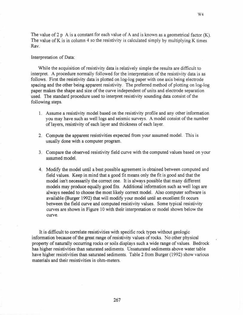
Table 2: List of resistivities of various materials (From Burger 1992)

\\:L"l III (110,-.1 l'L1YQ' ..,011 :JIll.! wet ..: 1ay

\ \ 'I.'[ I,) moi-.[ sill : suil J.no ",illY clay

\\ '1.' [ I, ) 1Tl00,t ... dt~ and ".muy soil,

\;.tlld .1I}(j grtJvd v. Lth I. lyl.'r, uj" ",iii

Co;.tr'l' dry ... and :.llld gLHt.:! JCfX1'lh

\\'cll-!rauurcd In ... lIght! ) fr;JcturcJ ni<...k v.ith nlOi'\· ... 'lij· filkJ cr~ lcb

<-ihghtly fr;.H.:turcJ [I)(.;\., v.ilh Jry, 'nil -fdkJ l,.:r'IL" \... '

\b.."j\d:- hcdJcu ro,:\...

MAGNETIC METHOD

Applications

J:., to II h

l .ow lOs ]( hl(11 00 ...

Low IOO()",

High IIX~"

IIXh Low IIXX),

High IIXXh

W4

A magnetometer measures changes in the earth's magnetic field strength. Any magnetic object that alters the earth's magnetic field can potentially be detected by magnetic surveying. Traditionally magnetic surveys have resulted in the construction of magnetic maps that show patterns diagnostic of a particular rock assemblage thus the method was useful in geologic mapping. The method has also been used to estimate depth to Precambrian basement by oil companies. More recent applications are the use of magnetics to detect buried steel tanks and drums containing hazardous waste materials. Archeologists have also found the method useful for locating cultural features with anomal ies being due to ferrous metals, hearths, and !cilms.

Magnetometers also have the option of measuring the vertical magnetic gradient which has several advantages over the use of total field measurements. Near surface sources of magnetic anomalies are accentuated over deeper regional bodies by the gradient measurements. The magnetic gradient also exhibits superior resolving power. This combined effect is important in locating lithologic contacts and shallow buried steel drums. Magnetic gradient data also aids in the interpretation of the physical characteristics of the source.

Equipment

A portable proton magnetometer with gradiometer option G856 AX will be used to conduct a magnetic survey over a small area or campus. The magnetometer reads and displays total magnetic field strengths (gammas) at the touch of a button. The readings are stored along with time, date and station number. The data is then fed into a computer and a printout may be obtained. A computer program MAGLOC and a contouring program can be used to plot magnetic contour maps based on the data.

269

W4

The magnetometer can be used to measure magnetic gradient by adding a second sensor. The two vertically separated sensors result in a measurement of the vertical magnetic gradient. Two 55 gallon steel drums are buried on campus for anyone who would like to try locating them by making gradient measurements.

WORKSHOP SCHEDULE EXPLORA nON GEOPHYSICS

The workshop on exploration geophysics will convene in the Geology Department at Potsdam College at 9:00 a.m., Sunday, September 26,1993 . Participants should report to Room 120 in Timerrnan Hall to have a brief discussion of the geophysical methods included in the workshop. Following the discussion geophysical equipment will be carried to the field behind Timerrnan Hall where the seismic refraction, electrical resistivity and magnetic surveys will be conducted.

After completion of the field survey, participants will return to Timerrnan Hall room 120 to analyze and interpret the field data. A demonstration of using the microcomputer to analyze and model the field data will be presented. Finally a discussion of the interpretation of the field data will be conducted. Participants will receive handouts on the geophysical methods of surveying conducted in the workshop. The workshop should be completed at 12:00 noon however participants are free to leave at any time.

REFERENCES CITED

Breiner, S. 1973, Applications Manual for Portable Magnetometers GeoMetrics p 58

Burger, H.R ., 1992 Exploration Geophysics of the Shallow Subsurface: Prentice Hall p.489

Dobrim, M.D., 1976 Introduction to Geophysical Prospecting ,McGraw-Hill Book Co. p 630

Goodacre, A.K. 1986 Interpretations of Gravity and Magnetic Anomalies for non-specialists Geological Survey of Canada: Geophysics Division p 361

Mooney, H.M., 1973 Handbook of Engineering Geophsyics Seismic Refraction, Bison Instruments

Mooney, H.M., 1980 Handbook of Engineering Geophysics Vol. 2 Electrical Resistivity, Bison Instruments Inc.

Nettleton, L.L., 1940 Geophysical Prospecting for Oil, McGraw-Hill p. 439

270

W4

Redpath, B.B., 1973 Seismic Refraction Exploration for Engineering Site Investigations, U.S. Department of Commerce. National Technical Information Service p. 51

Redpath, B and Scott, J. , and Huggins, R., 1991 GeoMetrics Short Course in Seismic Refraction Surveying: GeoMetrics

Robinson, E.S. and Coruh, C., 1988 Basic Exploration Geophysics: John Wiley and Sons p. 562

Woollard, G.P. and Hanson, G.F., 1954 Geophysical Methods Applied to Geologic Problems in Wisconsin, Bulletin No. 78, Wisconsin Geological Survey p. 254

271