A Two-Stage Robust Approach for the Reliable

Logistics Network Design Problem

Chun Chenga,b,c, Mingyao Qic,∗, Ying Zhangd, Louis-Martin Rousseaua,b

a Department of Mathematics and Industrial Engineering, Polytechnique Montreal, Montreal H3C 3A7, Canadab CIRRELT, Montreal H3C 3A7, Canada

c Research Center on Modern Logistics, Graduate School at Shenzhen, Tsinghua University, Shenzhen 518055, Chinad Zhejiang Cainiao Supply Chain Management Co., Ltd., Hangzhou 310000, China

Abstract

This paper examines a three-echelon logistics network in which all supply and transshipment nodes are subjectto disruption. We use uncertainty sets to describe the possible scenarios without depending on probabilisticinformation. We adopt a two-stage robust optimization approach where location decisions are made beforeand recourse decisions are made after the disruptions are known. We construct three two-stage robust models,which are solved exactly by a column-and-constraint-generation algorithm. Numerical tests demonstrate that theproposed algorithm outperforms the Benders decomposition method in both solution quality and computationaltime, and that the system’s reliability can be improved with only a slight increase in the normal cost.

Keywords: Reliable logistics network design; facility disruption; two-stage robust optimization; column-and-constraint-generation algorithm

1 Introduction

The logistics network design problem (LNDP) is key to achieving efficient operations among suppliers,

manufacturers, and customers (Min and Zhou 2002). Compared to the classical facility location prob-

lem, it considers multiple echelons and decides the number of suppliers and warehouses, their locations

and capacities, and the product flow throughout the network (Pishvaee et al. 2010). The LNDP deci-

sions are strategic: once facilities are built, they are expected to run long term, because it is normally

expensive to open and close facilities. Tactical (e.g., supplier and distribution channel selections) and

operational (e.g., vehicle scheduling) decisions are based on strategic decisions. Therefore, the value

of logistics network design is acknowledged in both academia and industry (Cordeau et al. 2006, Peng

et al. 2011, Melo et al. 2009).

One importance aspect in LNDP is to deal with uncertainty, like uncertain set-up costs of facilities,

uncertain transportation costs and customer demands (Alumur et al. 2012, Miskovic et al. 2017).

Corresponding author. E-mail address: qimy@sz.tsinghua.edu.cn

1

Facility disruption is another type of uncertainty. Natural disasters (earthquakes, hurricanes, etc.) or

industrial accidents (traffic or power interruption, etc.) can cause carefully constructed facilities to be

partially or completely destroyed, which may result in higher recourse/mitigation costs. Even minor

disruptions can have a significant impact on sales growth and stock returns, and it normally takes a

long time for companies to recover (Snyder et al. 2016). Therefore, many authors, including Snyder

and Daskin (2005), Cui et al. (2010), An et al. (2014), and Zhang et al. (2015), suggest considering

disruptions and the corresponding recourse operations in the system design phase.

Several probability-based models have been proposed (Snyder and Daskin 2005, 2006, Cui et al.

2010, Chen et al. 2011, Shen et al. 2011, Teimuory et al. 2013, Qin et al. 2013, Xie et al. 2015).

However, in many situations, it is impossible to obtain or predict precise probability information; there

may be insufficient historical data or no accurate forecasting method (An et al. 2014, Snyder et al.

2016). For instance, it is difficult to predict earthquakes. Robust optimization (RO) has been proposed

to deal with data uncertainty; it does not require probability information because uncertainty sets are

employed to capture randomness. It derives solutions that are robust to any disruptions within the

set. The static RO method makes decisions here and now, which could be overly conservative and

costly. However, the two-stage RO approach is able to generate less conservative solutions, because it

makes recourse decisions based on observed information. Therefore, it has been used to model unit

commitment problems in the power industry (An and Zeng 2015), location–transportation problems

(Zeng and Zhao 2013), and p-median facility location problems (An et al. 2011).

In this paper, we use a two-stage RO scheme for a network design problem that considers disruption.

In the first stage, we make location decisions based on any realization in the uncertainty set; and in the

second stage we make recourse decisions based on the first-stage location decisions and the revealed

uncertainty. Our study makes the following contributions:

(i) To the best of our knowledge, this paper is the first to solve the reliable LNDP using a two-stage

RO approach, which is able to produce less conservative solutions.

(ii) The RO model can be extended to include multiple uncertainty sets and impose upper bounds on

the worst-case performance of these sets. It can also be extended to partial disruptions.

(iii) We present an exact algorithm that outperforms the Benders decomposition (BD) method. We

present management insights based on the numerical results.

The rest of this paper is organized as follows. Section 2 reviews the literature. Section 3 describes

our problem and presents three two-stage RO models. Section 4 introduces an exact algorithm for

2

the models, and Section 5 presents the numerical results. Section 6 concludes the paper and suggests

future research directions.

2 Literature review

Supply chain disruption is not a new concept; it has existed as long as the supply chain itself. However,

in recent years it has received increasing attention. Snyder et al. (2016) give four reasons for the

explosion of interest: (1) high-profile events, such as the 9/11 terrorist attack in the United States

and the Japanese earthquake, have brought disruption to the forefront of public attention; (2) the

“just in time” concept leaves little room for adjustment, and this significantly exacerbates the impact

of disruption; (3) with the development of the global supply chain, suppliers are more integrated and

some are located in economically or politically unstable regions; (4) as with any other maturing research

area, scholars study this topic because of its high profile.

Drezner (1987) was the first to present mathematical models for location problems with unreliable

facilities. In the unreliable p-median problem (PMP) a facility has a given probability of becoming

inactive; in the (p, q)-center problem p facilities need to be built and at most q of them will fail

simultaneously. Snyder and Daskin (2005) study the reliable PMP and the reliable uncapacitated

fixed-charge location problem (UFLP), assuming that each facility that can fail has the same failure

probability. Cui et al. (2010) investigate the reliable UFLP and assume that each facility has a site-

dependent failure probability. Li and Ouyang (2010) further suppose that the facilities are subject to

spatially correlated disruptions. Lim et al. (2010) consider a facility location problem with two types of

facilities: unreliable facilities may fail with a probability in the failure state; and reliable facilities will

not fail but have higher fixed costs. Rayat et al. (2017) solve a multi-product and multi-period reliable

location-inventory-routing problem, where an unreliable distribution center (DC) has a possibility to be

disrupted in each period. Farahani et al. (2017) consider a multi-product location-inventory problem.

They assume that product k may be out of stock when facility j is partially disrupted, and customers

can purchase substitute products from facility j or try another facility to obtain the same product. For

more details on the reliable facility location problem see Snyder et al. (2016) and Sawik et al. (2018).

Although supply chain disruption has received extensive attention, research into disruption in the

context of network design is scarce (Snyder et al. 2016). The reliable LNDP extends the reliable facility

location problem by considering multiple echelons and allowing transshipment nodes in addition to

supplier and demand nodes. Both the supplier and transshipment nodes can be destroyed. It also

3

considers facility capacities.

Snyder et al. (2006) propose several scenario-based models (each scenario has an occurrence proba-

bility) for designing supply chains that are resilient to disruption. They first present a reliable network

design model for a network that will be built from scratch. For existing networks, they provide forti-

fication models and indicate that the reliability of the existing facilities can be enhanced by investing

in protection and security measures. Peng et al. (2011) study a reliable LNDP with a p−robustness

criterion, the objective of which is to minimize the nominal cost. They propose a scenario-based mixed-

integer programming (MIP) model and develop a hybrid genetic algorithm. In their numerical tests

they randomly generate several scenarios, where each facility has a 10% probability of becoming dis-

abled. Azad et al. (2013) consider a capacitated supply chain network design (SCND) model in which

both the facilities and the transportation network have a given probability of disruption. They assume

that the facilities are partially destroyed when disruptions occur and that the customers of a disrupted

DC are not assigned to other DCs; instead, the capacity lost at the disrupted DC is replenished from

non-disrupted DCs. They formulate a linear MIP model and propose a modified BD method. Shishe-

bori et al. (2014) study a reliable facility location/network design problem with a constraint on the

maximum allowable failure cost. The facilities and network links are assumed to be uncapacitated.

At most one facility fails at a time, and the demand nodes served by the disrupted facility must be

reallocated to the nearest surviving facility. The objective is to minimize the transportation cost.

Upper bounds are imposed on the investment in facility location and link construction. The authors

use a heuristic to solve a MIP model. Rezapour et al. (2017) study the influence of disruptions on the

competitiveness of supply chains and propose three policies to mitigate the disruption risk.

RO captures data randomness via uncertainty sets. An et al. (2014) use two-stage RO to model

both the uncapacitated and capacitated PMP with disruption considerations, and they minimize the

weighted sum of the normal cost and the worst-case cost. Zeng and Zhao (2013) construct a two-stage

RO model for the location–transportation problem with demand uncertainty. Baron et al. (2011) apply

RO to a multi-period fixed-charge network location problem with uncertain demands, and they explore

the influence of various uncertainty sets on the system decisions. Pishvaee et al. (2011) use RO to

handle the uncertainty of the input data in a closed-loop SCND problem. Parvaresh et al. (2014) apply

RO to a reliable hub network design problem.

Several algorithms have been developed for two-stage RO models: the approximation algorithm

(Atamturk and Zhang 2007, Bertsimas et al. 2011), BD (Jiang et al. 2012, Gabrel et al. 2014), and

column-and-constraint-generation (C&CG; Zeng and Zhao 2013, An et al. 2014, An and Zeng 2015).

4

For approximation algorithms, the second-stage decisions should be simple functions or have special

characteristics to ensure that the problem is manageable. The computational time of the BD method

increases significantly with increasing instance size. However, the C&CG algorithm has proved to be

efficient for two-stage RO models (Zeng and Zhao 2013). Therefore, we use this algorithm, and we

develop an enhancement technique to further improve its computational efficiency.

Thus, our paper differs from those on the reliable PMP and UFLP by considering multiple echelons

and facility capacities. Specifically, our work differs from An et al. (2015) and An and Zeng (2015)

in following aspects: (1) An et al. (2015) focus on analyzing the structural properties of the robust

PMP and exploring the modeling capability of two-stage RO by considering partial disruption and

demand changes (this is possible because the facility set and the customer set is the same in their

paper). However, we extend the basic RO scheme to include multiple uncertainty sets to characterize

decision makers’ conservative level. And the model in An et al. (2015) can be recognized as a special

case of this modeling scheme. We also introduce upper bounds for the worst-case performance, and

this modeling framework can be used as a decision support tool for system expansion with reliability

considerations. Our numerical tests demonstrate that the new models can generate less conservative

solutions. (2) An and Zeng (2015) present robust unit commitment models, where the load is subject

to interval uncertainty. They focus on building the connection between the robust models and the

stochastic models. However, we apply the modeling scheme to a reliable LNDP and explain the

connections and differences among various models. Extensive numerical tests are conducted to study

the conservativeness of different models and the price of robustness. Values of key parameters are also

analyzed to provide insights for supply chain decision-makers.

3 Model formulation

In this section, we first introduce our notation. We then present a basic two-stage RO model for the

reliable LNDP and explore the modeling capability of two-stage RO by describing two variants of the

basic model: the expanded robust LNDP model and the risk-constrained robust LNDP model.

3.1 Notation

3.1.1 Parameters

Consider a general network (V,A). Let VS , VT , and VD be the sets of supply, transshipment, and

demand nodes. Define V0 = VS ∪ VT to be the set of facilities for which open/close decisions are

5

required, and V = V0 ∪ VD.

The other parameters are as follows:

• fj = fixed cost to open facility j ∈ V0

• cij = unit transportation cost on arc (i, j) ∈ A

• Qj = capacity of facility j ∈ V0

• bj = supply of node j ∈ V; bj ≥ 0 if j ∈ VS , bj = 0 if j ∈ VT , and bj ≤ 0 if j ∈ VD.

• θi = unit penalty cost for unsatisfied demand at node i ∈ VD

3.1.2 Decision variables

The decisions are made in two stages. We make location decisions at the first stage. After the

disruption, we implement recourse or mitigation operations at the second stage: reassigning demand

nodes to surviving facilities to ensure system reliability. We use y and x, u to represent the first- and

second-stage decision variables respectively, i.e.,

• yj = 1 if facility j ∈ V0 is opened in the first stage, yj = 0 otherwise

• xij = product flow on arc (i, j) in a specific disruptive scenario

• ui = unsatisfied demand at node i ∈ VD in a specific disruptive scenario

Our two-stage robust optimization model uses a budgeted uncertainty set to describe possible dis-

ruptive scenarios without requiring any probabilistic information. We assume that at most m facilities

fail simultaneously:

A =

z ∈ {0, 1}|V0| :∑j∈V0

zj ≤ m

, (1)

where zj = 1 if facility j is disrupted and zj = 0 otherwise.

3.2 Formulations

We first present the basic two-stage RO model, in which only one uncertainty set is considered. Then

we introduce two models with multiple uncertainty sets.

3.2.1 Basic two-stage RO model

We formulate the basic two-stage RO LNDP model as follows, where V+i = {j ∈ V|(i, j) ∈ A} and

V−i = {j ∈ V|(j, i) ∈ A}.

6

RO-LNDP0:

miny

∑j∈V0

fjyj + maxz∈A

minx,u∈S(y,z)

(∑

(i,j)∈A

cijxij +∑j∈VD

θjuj) (2)

s.t.

yj ∈ {0, 1} ∀j ∈ V0 (3)

Here S(y, z) = {

∑i∈V+

j

xji ≤ bj ∀j ∈ VS (4)

∑i∈V+

j

xji =∑i∈V−j

xij ∀j ∈ VT (5)

∑i∈V−j

xij + uj = −bj ∀j ∈ VD (6)

∑i∈V+

j

xji ≤ (1− zj)Qjyj ∀j ∈ V0 (7)

xij ≥ 0 ∀(i, j) ∈ A (8)

uj ≥ 0 ∀j ∈ VD} (9)

The objective function in (2) minimizes the cost of the worst-case scenario. The max operator

represents the disruptive scenario in A that generates the largest recourse cost, given the facility

locations y. The min operator identifies the least costly solution, and the set S(y, z) represents

possible recourse operations. Constraints (4)–(6) are the product flow conservation equations for all

nodes. Constraints (7) ensure that when a facility is open and functional the flow does not exceed its

capacity, and they prohibit any flow when it is closed or destroyed. Constraints (3), (8), and (9) define

the variable types.

3.2.2 Expanded two-stage RO model

Two key factors influence the solution of the two-stage RO: the uncertainty set and the worst-case

performance. A small uncertainty set cannot adequately capture the random factor; a large set leads

to solutions that are costly and overly conservative. To deal with this, An and Zeng (2015) suggest

using multiple uncertainty sets and assigning different weights to the worst-case performances of these

sets. Our RO-LNDP0 model can be extended to multiple uncertainty sets as follows:

7

RO-LNDP1:

miny

∑j∈V0

fjyj +

K∑k=1

ρk

maxz∈Ak

minx,u∈Sk(y,z)

(∑

(i,j)∈A

cijxij +∑j∈VD

θjuj)

(10)

where y and Sk(y, z) are defined by constraints (3) and (4)–(9), respectively. In the objective function

(10), Ak denotes the kth uncertainty set, with weight ρk (0 ≤ ρk ≤ 1 and∑

k ρk = 1).

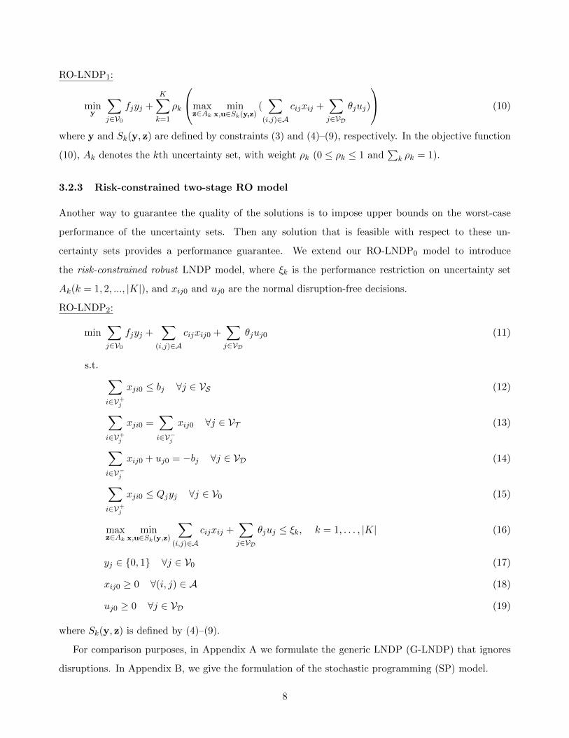
3.2.3 Risk-constrained two-stage RO model

Another way to guarantee the quality of the solutions is to impose upper bounds on the worst-case

performance of the uncertainty sets. Then any solution that is feasible with respect to these un-

certainty sets provides a performance guarantee. We extend our RO-LNDP0 model to introduce

the risk-constrained robust LNDP model, where ξk is the performance restriction on uncertainty set

Ak(k = 1, 2, ..., |K|), and xij0 and uj0 are the normal disruption-free decisions.

RO-LNDP2:

min∑j∈V0

fjyj +∑

(i,j)∈A

cijxij0 +∑j∈VD

θjuj0 (11)

s.t. ∑i∈V+

j

xji0 ≤ bj ∀j ∈ VS (12)

∑i∈V+

j

xji0 =∑i∈V−j

xij0 ∀j ∈ VT (13)

∑i∈V−j

xij0 + uj0 = −bj ∀j ∈ VD (14)

∑i∈V+

j

xji0 ≤ Qjyj ∀j ∈ V0 (15)

maxz∈Ak

minx,u∈Sk(y,z)

∑(i,j)∈A

cijxij +∑j∈VD

θjuj ≤ ξk, k = 1, . . . , |K| (16)

yj ∈ {0, 1} ∀j ∈ V0 (17)

xij0 ≥ 0 ∀(i, j) ∈ A (18)

uj0 ≥ 0 ∀j ∈ VD (19)

where Sk(y, z) is defined by (4)–(9).

For comparison purposes, in Appendix A we formulate the generic LNDP (G-LNDP) that ignores

disruptions. In Appendix B, we give the formulation of the stochastic programming (SP) model.

8

3.2.4 Summary of models and another extension

The connections and differences among models are shown in Figure 1 and Table 1. The G-LNDP model

is a special case of the RO-LNDP0 model with m = 0, and also a special case of the RO-LNDP1 model

with K = 1 and m = 0. The RO-LNDP1 model reduces to the RO-LNDP0 model when K = 1 and

m > 0. Furthermore, An and Zeng (2015) have proved that the RO-LNDP1 model is equivalent to the

SP model when the uncertainty sets are individual scenarios. The RO-LNDP2 model reduces to the

G-LNDP model when the performance bound ξk is sufficiently large.

RO-LNDP0

RO-LNDP1

RO-LNDP2

G-LNDP

! = 0

$ = 1,! = 0

ξ& is unbounded

$ = 1,! > 0

SP model

uncertainty sets areindividual scenarios

Figure 1: Connections among models

From Table 1, our three two-stage robust models differ in the number of uncertainty sets and the

objective function. The basic RO model has one uncertainty set, and the other models have multiple

uncertainty sets. The objective of the basic RO model is to minimize the cost of the worst-case scenario

in the uncertainty set. The expanded RO model identifies the worst-case scenario in each uncertainty

set and minimizes the weighted sum. The risk-constrained RO model minimizes the cost of the normal

disruption-free situation.

Table 1: Model comparison

Model Possibility information

required?

Uncertainty

set/scenarios

Objective (minimize cost)

Generic LNDP Not applicable Not applicable Normal disruption-free case

Basic RO No One Worst-case

Expanded RO No Multiple Weighted sum of multiple worst-cases

Risk-constrained RO No Multiple Normal disruption-free case

Stochastic programming Yes Multiple Weighted sum of multiple scenarios

Another extension of our work allows partial disruption in which a damaged facility can still satisfy

part of the demand. We introduce a parameter δj (0 < δj ≤ 1) to represent the change in facility j’s

9

capacity in a disruptive scenario, and constraints (7) become

∑i∈V+

j

xji ≤ (1− δjzj)Qjyj ∀j ∈ V0 (20)

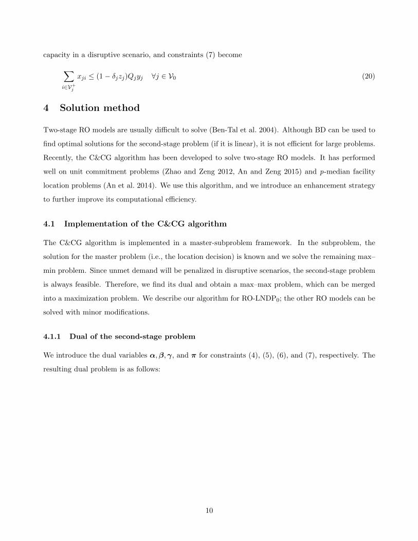
4 Solution method

Two-stage RO models are usually difficult to solve (Ben-Tal et al. 2004). Although BD can be used to

find optimal solutions for the second-stage problem (if it is linear), it is not efficient for large problems.

Recently, the C&CG algorithm has been developed to solve two-stage RO models. It has performed

well on unit commitment problems (Zhao and Zeng 2012, An and Zeng 2015) and p-median facility

location problems (An et al. 2014). We use this algorithm, and we introduce an enhancement strategy

to further improve its computational efficiency.

4.1 Implementation of the C&CG algorithm

The C&CG algorithm is implemented in a master-subproblem framework. In the subproblem, the

solution for the master problem (i.e., the location decision) is known and we solve the remaining max–

min problem. Since unmet demand will be penalized in disruptive scenarios, the second-stage problem

is always feasible. Therefore, we find its dual and obtain a max–max problem, which can be merged

into a maximization problem. We describe our algorithm for RO-LNDP0; the other RO models can be

solved with minor modifications.

4.1.1 Dual of the second-stage problem

We introduce the dual variables α,β,γ, and π for constraints (4), (5), (6), and (7), respectively. The

resulting dual problem is as follows:

10

NonL-SubP:

max∑j∈VS

bjαj −∑j∈VD

bjγj +∑j∈V0

(1− zj)Qj yjπj (21)

s.t.

αi + βj + πi ≤ cij ∀i ∈ VS , j ∈ VT ∩ V+i (22)

αi + γj + πi ≤ cij ∀i ∈ VS , j ∈ VD ∩ V+i (23)

− βi + γj + πi ≤ cij ∀i ∈ VT , j ∈ VD ∩ V+i (24)

γj ≤ θj ∀j ∈ VD (25)

αj ≤ 0 ∀j ∈ VS (26)

πj ≤ 0 ∀j ∈ V0 (27)

Since πj ≤ 0 and zj ∈ {0, 1}, the nonlinear term zjπj is the product of a binary variable and a

continuous variable. We can linearize it by introducing a new continuous variable wj = zjπj and using

a big-M method, with the following constraints:

wj ≥ πj (28)

wj ≥ −Mzj (29)

wj ≤ πj +M(1− zj) (30)

wj ≤ 0 (31)

The value of M can be set as follows: For each facility j ∈ V0 and demand node i ∈ VD, define c′ji as

the minimal cost from j to i, i.e., c′ji = min{cji, cjk + cki}, where k is a transshipment node. If there

is no arc between facility j and demand node i, then cji = +∞. Define M ′j = maxi∈VD{θi − c′ji} and

M ′′j = maxi∈V+j{cji}. Then we set

−πj ≤ max{M ′j ,M ′′j } = Mj j ∈ V0 (32)

Therefore, the linearized subproblem is:

L-SubP:

χ = max∑j∈VS

bjαj −∑j∈VD

bjγj +∑j∈V0

Qj yj(πj − wj) (33)

subject to constraints (22)–(31).

11

4.1.2 Framework of the C&CG algorithm

We now describe the framework of the C&CG algorithm and present the formulation of the master

problem (MP), which will be solved iteratively. At each iteration r, we identify a worst-case scenario

zr by solving the linearized subproblem. Then we create the recourse variables (xr,ur) and the cor-

responding constraints, as well as this specific scenario, and add them to the MP. Let LB and UB be

the lower and upper bounds, Gap = (UB−LB)/UB, and let the optimality tolerance be ε. The C&CG

algorithm is as follows:

(1) Set LB = -∞, UB = +∞, and r = 0.

(2) Take any arbitrary y ∈ {0, 1}|V0| as initial solution.

(3) Solve the linearized subproblem with regards to y to identify the worst-case scenario z. Update

r = r + 1. Create recourse variables (xr,ur) and corresponding constraints, and add them to the

following MP.

MP:

min∑j∈V0

fjyj + φ (34)

s.t.

φ ≥∑

(i,j)∈A

cijxlij +

∑j∈VD

θjulj ∀l = 1, 2, ..., r (35)

∑i∈V+

j

xlji ≤ bj ∀j ∈ VS ∀l = 1, 2, ..., r (36)

∑i∈V+

j

xlji =∑i∈V −j

xlij ∀j ∈ VT ∀l = 1, 2, ..., r (37)

∑i∈V−j

xlij + ulj = −bj ∀j ∈ VD ∀l = 1, 2, ..., r (38)

∑i∈V+

j

xlji ≤ (1− zlj)Qjyj ∀j ∈ V0 ∀l = 1, 2, ..., r (39)

yj ∈ {0, 1} ∀j ∈ V0 (40)

xlij ≥ 0 ∀(i, j) ∈ A ∀l = 1, 2, ..., r (41)

ulj ≥ 0 ∀j ∈ VD ∀l = 1, 2, ..., r (42)

(4) Iterate until the algorithm terminates:

(i) Solve the MP to find an optimal solution (y, φ); set LB to the optimal value of the MP.

12

(ii) Solve the subproblem with regards to y to identify the worst-case scenario z. Update UB =

min{

UB,∑

j∈V0 fjyrj + χr

}.

(iii) If Gap ≤ ε, terminate; otherwise, update r = r + 1 and create the recourse variables and

corresponding constraints. Add them to the MP and go to step (i).

We also implement BD, in which a single cutting plane

φ ≥∑j∈VS

bjαrj −

∑j∈VD

bjγrj +

∑j∈V0

(1− zrj )Qjyjπrj (43)

is iteratively added to the MP, which carries only the first-stage decision variable y.

Remarks: (1) for the RO-LNDP1 model, the objective function of the MP becomes

min∑j∈V0

fjyj +

K∑k=1

ρkφk (44)

where φk corresponds to the kth uncertainty set. For each uncertainty set, we need to solve a subprob-

lem to identify the worst-case scenario, and we add its recourse variables and corresponding constraints

to the MP.

(2) For the RO-LNDP2 model, at each iteration we solve a subproblem for each uncertainty set, to

check whether its worst-case performance violates the bound. Once there exists such scenarios, we add

all the identified worst-case scenarios to the MP until all the performance bounds are respected.

4.2 Algorithm enhancement

In this section we introduce a variable fixing technique to improve the algorithm’s performance. This

technique has been shown to be efficient in reducing the computational burden for facility location

problems (Snyder and Daskin 2005, Contreras et al. 2011, Zhang et al. 2016). We generalize it to solve

the reliable LNDP. The idea is as follows:

Let y be the incumbent solution with corresponding upper bound UB′.

• If yj = 0: we add an additional constraint yj = 1 to the MP and solve it to optimality; if its

optimal value is larger than UB′, then we fix yj to 0 in the MP.

• If yj = 1: we add an additional constraint yj = 0 to the MP and solve it to optimality; if its

optimal value is larger than UB′, then we fix yj to 1 in the MP.

To understand this technique, imagine that we choose to branch on variable yj with two branches

yj = 1 and yj = 0 in the branch-and-bound tree. Clearly, the solutions obtained from both nodes are

lower bounds for their children nodes, respectively. If the generated solution is larger than UB′, we

13

prune the tree at the corresponding node, because all of its children nodes will generate solutions that

are larger than UB′.

Fixing some yj reduces the feasible space of the MP, which can help improve computational efficiency.

On the other hand, each time a new constraint with yj = 1 or 0 is added, and this might increase the

computational time, especially when the number of facilities is large. Therefore, (1) after adding the

new constraint, we solve the corresponding linear relaxation and get a lower bound, and we compare

this bound with UB′ (“C&CG LP”); (2) we solve the MP with the new constraint to optimality and

compare the optimal value with UB′ (“C&CG Optimal”).

5 Numerical experiments and analyses

In this section, we present the instances, discuss our numerical tests, analyze the influence of the

parameters, and present some insights. The algorithm is coded in the C# programming language and

run on a PC with a 2.53 GHz Intel Core Dual Processor and 3 GB of memory. The MP and subproblem

are solved using Gurobi 6.0.

5.1 Instances

We randomly generate instances of different sizes. The method is based on that of Peng et al. (2011),

with a few modifications. The instances are labeled “d−|VS |−|VT |−|VD|,” where d is the edge density

(20%, 30%, or 50%) and |VS |, |VT |, and |VD| are the number of supply, transshipment, and demand

nodes. The number of nodes ranges from 60 to 100.

For each demand node j ∈ VD, the unmet-demand penalty is 1500, and the demand bj is drawn

uniformly from [−110,−50]. Let Sb = −∑

j∈VD bj be the sum of all the demands (the negative sign

appears because bj ≤ 0); define s = Sb|VS | and c = Sb

|VT | .

For each facility node j ∈ V0, the fixed cost is drawn uniformly from [5000, 15000]; if j ∈ VS , then

its capacity Qj is drawn uniformly from [1.5s, 2.5s] and its supply bj is the same as its capacity; if

j ∈ VT , then its capacity Qj is drawn uniformly from [1.5c, 2.5c] and its supply bj is 0.

The arcs are constructed based on the probability specified by the edge density. In detail, for two

nodes i, j (i ∈ VS , j ∈ VT or i ∈ VS , j ∈ VD or i ∈ VT , j ∈ VD) and edge density d, we generate a

random number r ∈ [0, 1]. If r ≤ d, then we construct an arc between i and j. The unit transportation

cost of each arc (i, j) ∈ A is drawn uniformly from [1, 500].

14

5.2 Algorithm performance

We now evaluate the performance of the algorithms. We set the maximal number of facilities that can

fail simultaneously to 5, i.e., m = 5 (we arbitrarily choose a large value for m to test the efficiency

of the C&CG algorithm). The facilities are destroyed completely when disruptions occur (i.e., δj =

1, ∀j ∈ V0). The model is RO-LNDP0, and the results are shown in Table 2. The optimality tolerance

ε is set to 10−6 and the time limit is 10800 seconds (when this limit is reached, the current iteration

will be completed). In Table 2, the results in the “C&CG No Fix” columns are obtained by using

the C&CG algorithm without enhancement. The column Iter gives the number of iterations; Time

indicates the computational time in seconds; and Gap is the relative percentage gap between the upper

and lower bounds.

Table 2 shows that for most instances (9 out of 13), the C&CG algorithm is hundreds of times faster

than BD, and the number of iterations is much lower. Within the time limit, BD can find optimal

solutions for just 3 instances. In contrast, the C&CG algorithm is able to generate optimal solutions

for most of the instances, and C&CG LP finds the optimal solution for all the instances. Therefore,

the C&CG algorithm outperforms BD in both computational time and solution quality.

To further demonstrate the superiority of C&CG LP, Figure 2 shows the convergence curves of the

two algorithms for the instance 20%-10-20-30. In Figure 2(a), the gap between the lower and upper

bounds reduces slowly and does not reach zero even after 1000 iterations; the C&CG LP algorithm

finds the optimal solution after 11 iterations. The instances 50%-20-20-30, 50%-30-20-30, and 50%-40-

20-30 show that the number of supply nodes has a significant impact on the computational efficiency.

For these instances, C&CG LP finds optimal solutions within the time limit and performs better than

C&CG No Fix and C&CG Optimal. Therefore, for our model comparison and parameter sensitivity

analysis, we use C&CG LP.

15

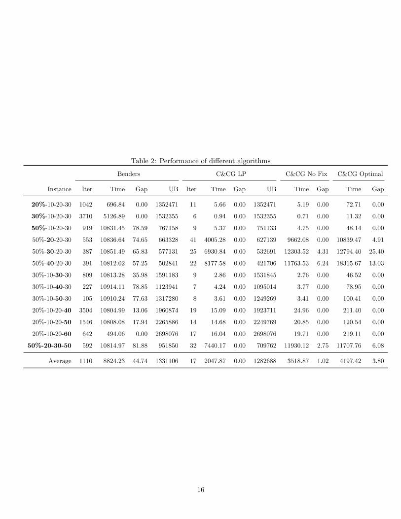
Table 2: Performance of different algorithms

Benders C&CG LP C&CG No Fix C&CG Optimal

Instance Iter Time Gap UB Iter Time Gap UB Time Gap Time Gap

20%-10-20-30 1042 696.84 0.00 1352471 11 5.66 0.00 1352471 5.19 0.00 72.71 0.00

30%-10-20-30 3710 5126.89 0.00 1532355 6 0.94 0.00 1532355 0.71 0.00 11.32 0.00

50%-10-20-30 919 10831.45 78.59 767158 9 5.37 0.00 751133 4.75 0.00 48.14 0.00

50%-20-20-30 553 10836.64 74.65 663328 41 4005.28 0.00 627139 9662.08 0.00 10839.47 4.91

50%-30-20-30 387 10851.49 65.83 577131 25 6930.84 0.00 532691 12303.52 4.31 12794.40 25.40

50%-40-20-30 391 10812.02 57.25 502841 22 8177.58 0.00 421706 11763.53 6.24 18315.67 13.03

30%-10-30-30 809 10813.28 35.98 1591183 9 2.86 0.00 1531845 2.76 0.00 46.52 0.00

30%-10-40-30 227 10914.11 78.85 1123941 7 4.24 0.00 1095014 3.77 0.00 78.95 0.00

30%-10-50-30 105 10910.24 77.63 1317280 8 3.61 0.00 1249269 3.41 0.00 100.41 0.00

20%-10-20-40 3504 10804.99 13.06 1960874 19 15.09 0.00 1923711 24.96 0.00 211.40 0.00

20%-10-20-50 1546 10808.08 17.94 2265886 14 14.68 0.00 2249769 20.85 0.00 120.54 0.00

20%-10-20-60 642 494.06 0.00 2698076 17 16.04 0.00 2698076 19.71 0.00 219.11 0.00

50%-20-30-50 592 10814.97 81.88 951850 32 7440.17 0.00 709762 11930.12 2.75 11707.76 6.08

Average 1110 8824.23 44.74 1331106 17 2047.87 0.00 1282688 3518.87 1.02 4197.42 3.80

16

0 200 400 600 800 10000

0.5

1

1.5

2

2.5

3

3.5x 10

6

Iterations

Cos

t

LBUB

500 600 700 800 900 1000

1.2

1.3

1.4

1.5

x 106

(a) Benders decomposition

0 2 4 6 8 100

0.5

1

1.5

2

2.5

3

3.5x 10

6

Iterations

Cos

t

LBUB

(b) C&CG

Figure 2: Convergence curves for instance 20%-10-20-30

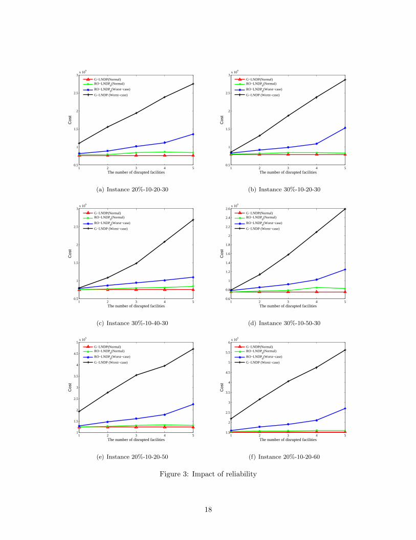
5.3 Impact of reliability

Obviously, if disruptions are not considered (i.e., G-LNDP), the system’s normal cost will be lower, but

it may be more expensive to implement mitigation/recourse operations when they become necessary.

To investigate the impact of reliability on the system cost, we conduct the following experiments:

(1) We solve RO-LNDP0 to find the location decision. We then fix this decision and solve a minimum

cost flow problem (MCFP) to find the system’s normal cost under RO-LNDP0. This indicates the

impact of disruptions on the system’s normal cost.

(2) We solve G-LNDP and fix the location decision. We then solve the slave problem of the C&CG

algorithm to identify the worst-case cost. This indicates the cost of not considering disruptions in

advance and handling them as they occur.

For space considerations, Figure 3 shows the curves of just 6 instances. The results for the other

instances are similar. Figure 3 confirms that considering disruptions will increase the normal cost.

However, ignoring disruptions during the design phase leads to higher costs when they do occur. As m

increases, the deviation of the worst-case cost for RO-LNDP0 and G-LNDP also increases. However,

the normal cost of these two models is similar. We conclude that the two-stage RO model gives a

considerable decrease of the recourse cost in the worst disruptive situation with only a small increase

in the normal cost.

17

1 2 3 4 50.5

1

1.5

2

2.5

3x 10

6

The number of disrupted facilities

Cos

t

G−LNDP(Normal)RO−LNDP

0(Normal)

RO−LNDP0(Worst−case)

G−LNDP (Worst−case)

(a) Instance 20%-10-20-30

1 2 3 4 50.5

1

1.5

2

2.5

3x 10

6

The number of disrupted facilities

Cos

t

G−LNDP(Normal)RO−LNDP

0(Normal)

RO−LNDP0(Worst−case)

G−LNDP (Worst−case)

(b) Instance 30%-10-20-30

1 2 3 4 50.5

1

1.5

2

2.5

3x 10

6

The number of disrupted facilities

Cos

t

G−LNDP(Normal)RO−LNDP

0(Normal)

RO−LNDP0(Worst−case)

G−LNDP (Worst−case)

(c) Instance 30%-10-40-30

1 2 3 4 50.6

0.8

1

1.2

1.4

1.6

1.8

2

2.2

2.4

2.6x 10

6

The number of disrupted facilities

Cos

t

G−LNDP(Normal)RO−LNDP

0(Normal)

RO−LNDP0(Worst−case)

G−LNDP (Worst−case)

(d) Instance 30%-10-50-30

1 2 3 4 51

1.5

2

2.5

3

3.5

4

4.5

5x 10

6

The number of disrupted facilities

Cos

t

G−LNDP(Normal)RO−LNDP

0(Normal)

RO−LNDP0(Worst−case)

G−LNDP (Worst−case)

(e) Instance 20%-10-20-50

1 2 3 4 51.5

2

2.5

3

3.5

4

4.5

5

5.5

6x 10

6

The number of disrupted facilities

Cos

t

G−LNDP(Normal)RO−LNDP

0(Normal)

RO−LNDP0(Worst−case)

G−LNDP (Worst−case)

(f) Instance 20%-10-20-60

Figure 3: Impact of reliability

18

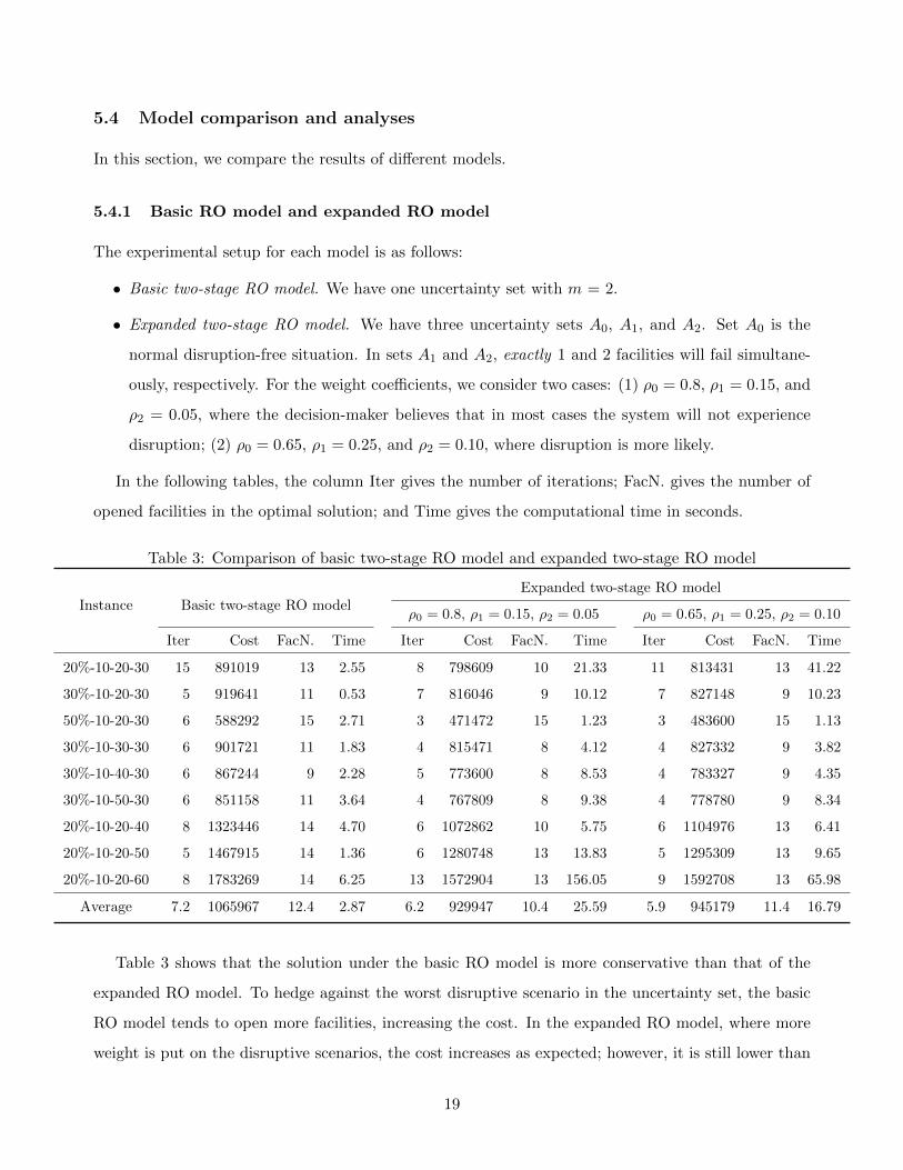
5.4 Model comparison and analyses

In this section, we compare the results of different models.

5.4.1 Basic RO model and expanded RO model

The experimental setup for each model is as follows:

• Basic two-stage RO model. We have one uncertainty set with m = 2.

• Expanded two-stage RO model. We have three uncertainty sets A0, A1, and A2. Set A0 is the

normal disruption-free situation. In sets A1 and A2, exactly 1 and 2 facilities will fail simultane-

ously, respectively. For the weight coefficients, we consider two cases: (1) ρ0 = 0.8, ρ1 = 0.15, and

ρ2 = 0.05, where the decision-maker believes that in most cases the system will not experience

disruption; (2) ρ0 = 0.65, ρ1 = 0.25, and ρ2 = 0.10, where disruption is more likely.

In the following tables, the column Iter gives the number of iterations; FacN. gives the number of

opened facilities in the optimal solution; and Time gives the computational time in seconds.

Table 3: Comparison of basic two-stage RO model and expanded two-stage RO model

Instance Basic two-stage RO modelExpanded two-stage RO model

ρ0 = 0.8, ρ1 = 0.15, ρ2 = 0.05 ρ0 = 0.65, ρ1 = 0.25, ρ2 = 0.10

Iter Cost FacN. Time Iter Cost FacN. Time Iter Cost FacN. Time

20%-10-20-30 15 891019 13 2.55 8 798609 10 21.33 11 813431 13 41.22

30%-10-20-30 5 919641 11 0.53 7 816046 9 10.12 7 827148 9 10.23

50%-10-20-30 6 588292 15 2.71 3 471472 15 1.23 3 483600 15 1.13

30%-10-30-30 6 901721 11 1.83 4 815471 8 4.12 4 827332 9 3.82

30%-10-40-30 6 867244 9 2.28 5 773600 8 8.53 4 783327 9 4.35

30%-10-50-30 6 851158 11 3.64 4 767809 8 9.38 4 778780 9 8.34

20%-10-20-40 8 1323446 14 4.70 6 1072862 10 5.75 6 1104976 13 6.41

20%-10-20-50 5 1467915 14 1.36 6 1280748 13 13.83 5 1295309 13 9.65

20%-10-20-60 8 1783269 14 6.25 13 1572904 13 156.05 9 1592708 13 65.98

Average 7.2 1065967 12.4 2.87 6.2 929947 10.4 25.59 5.9 945179 11.4 16.79

Table 3 shows that the solution under the basic RO model is more conservative than that of the

expanded RO model. To hedge against the worst disruptive scenario in the uncertainty set, the basic

RO model tends to open more facilities, increasing the cost. In the expanded RO model, where more

weight is put on the disruptive scenarios, the cost increases as expected; however, it is still lower than

19

that of the basic RO model.

The computational time is slightly higher for the expanded RO model than the basic RO model.

However, with CC&G LP, the expanded model can still be solved to optimality in a short time.

5.4.2 Expanded RO model and stochastic programming model

We select instances 20%-10-20-30, 30%-10-20-30, 50%-10-20-30, 20%-10-20-40, 20%-10-20-50, and 20%-

10-20-60 for these analyses, and the number of facilities is 30. For the expanded two-stage RO model,

we use three uncertainty sets as in Section 5.4.1, and the weight coefficients are ρ0 = 0.74, ρ1 = 0.22,

and ρ2 = 0.04. For the SP model, the failure probability of each facility is set to 0.01, which roughly

matches the weight of each uncertainty set in the expanded RO model: the probability is 0.740 for the

normal disruption-free situation, 0.224 for the scenario with exactly 1 facility disrupted, and 0.033 for

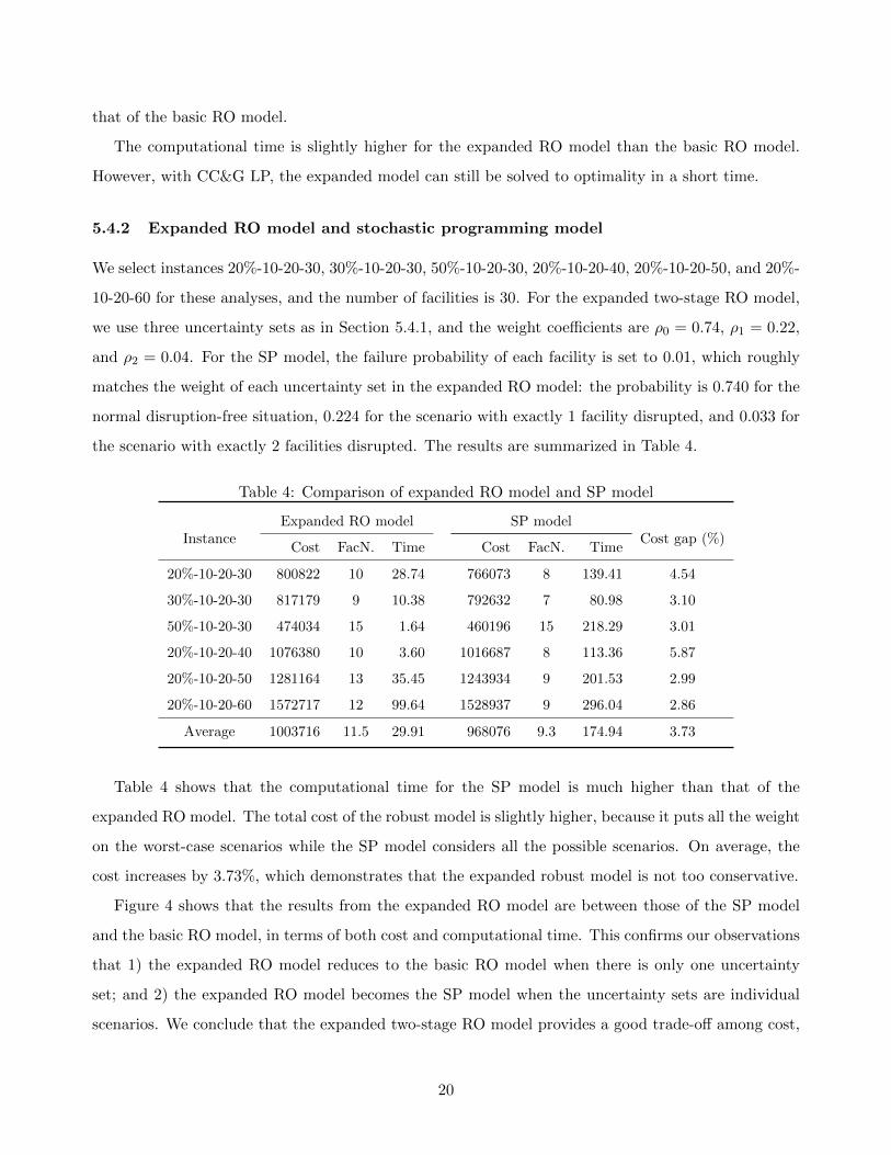
the scenario with exactly 2 facilities disrupted. The results are summarized in Table 4.

Table 4: Comparison of expanded RO model and SP model

InstanceExpanded RO model SP model

Cost gap (%)Cost FacN. Time Cost FacN. Time

20%-10-20-30 800822 10 28.74 766073 8 139.41 4.54

30%-10-20-30 817179 9 10.38 792632 7 80.98 3.10

50%-10-20-30 474034 15 1.64 460196 15 218.29 3.01

20%-10-20-40 1076380 10 3.60 1016687 8 113.36 5.87

20%-10-20-50 1281164 13 35.45 1243934 9 201.53 2.99

20%-10-20-60 1572717 12 99.64 1528937 9 296.04 2.86

Average 1003716 11.5 29.91 968076 9.3 174.94 3.73

Table 4 shows that the computational time for the SP model is much higher than that of the

expanded RO model. The total cost of the robust model is slightly higher, because it puts all the weight

on the worst-case scenarios while the SP model considers all the possible scenarios. On average, the

cost increases by 3.73%, which demonstrates that the expanded robust model is not too conservative.

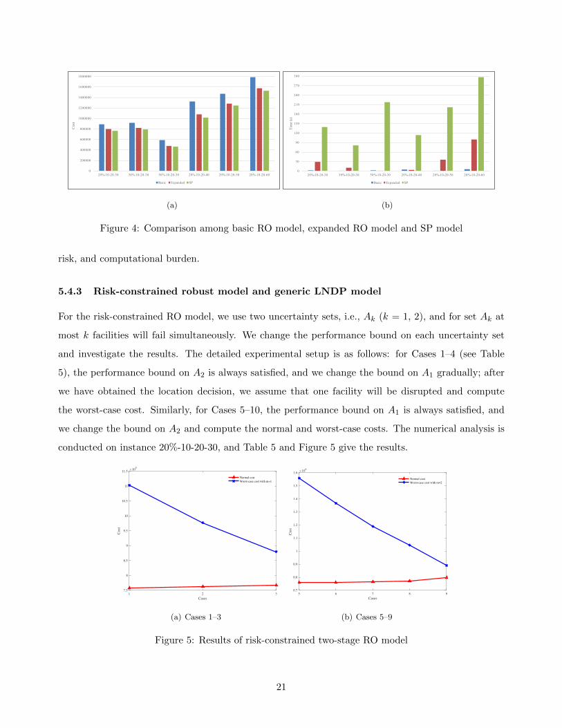
Figure 4 shows that the results from the expanded RO model are between those of the SP model

and the basic RO model, in terms of both cost and computational time. This confirms our observations

that 1) the expanded RO model reduces to the basic RO model when there is only one uncertainty

set; and 2) the expanded RO model becomes the SP model when the uncertainty sets are individual

scenarios. We conclude that the expanded two-stage RO model provides a good trade-off among cost,

20

0

200000

400000

600000

800000

1000000

1200000

1400000

1600000

1800000

20%-10-20-30 30%-10-20-30 50%-10-20-30 20%-10-20-40 20%-10-20-50 20%-10-20-60

Cost

Basic Expanded SP

(a)

0

30

60

90

120

150

180

210

240

270

300

20%-10-20-30 30%-10-20-30 50%-10-20-30 20%-10-20-40 20%-10-20-50 20%-10-20-60

Time(s)

Basic Expanded SP

(b)

Figure 4: Comparison among basic RO model, expanded RO model and SP model

risk, and computational burden.

5.4.3 Risk-constrained robust model and generic LNDP model

For the risk-constrained RO model, we use two uncertainty sets, i.e., Ak (k = 1, 2), and for set Ak at

most k facilities will fail simultaneously. We change the performance bound on each uncertainty set

and investigate the results. The detailed experimental setup is as follows: for Cases 1–4 (see Table

5), the performance bound on A2 is always satisfied, and we change the bound on A1 gradually; after

we have obtained the location decision, we assume that one facility will be disrupted and compute

the worst-case cost. Similarly, for Cases 5–10, the performance bound on A1 is always satisfied, and

we change the bound on A2 and compute the normal and worst-case costs. The numerical analysis is

conducted on instance 20%-10-20-30, and Table 5 and Figure 5 give the results.

1 2 3Cases

7.5

8

8.5

9

9.5

10

10.5

11

11.5

Cos

t

#105

Normal costWorst-case cost with m=1

(a) Cases 1–3

5 6 7 8 9Cases

0.7

0.8

0.9

1

1.1

1.2

1.3

1.4

1.5

1.6

Cos

t

#106

Normal costWorst-case cost with m=2

(b) Cases 5–9

Figure 5: Results of risk-constrained two-stage RO model

21

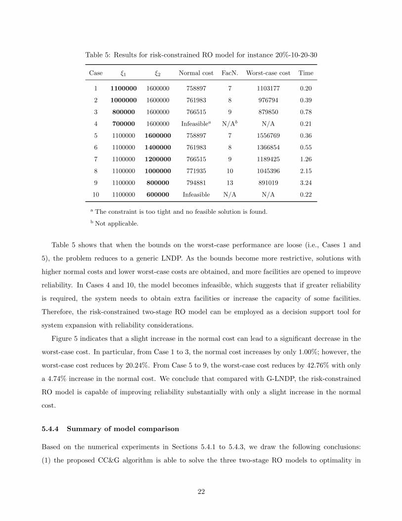
Table 5: Results for risk-constrained RO model for instance 20%-10-20-30

Case ξ1 ξ2 Normal cost FacN. Worst-case cost Time

1 1100000 1600000 758897 7 1103177 0.20

2 1000000 1600000 761983 8 976794 0.39

3 800000 1600000 766515 9 879850 0.78

4 700000 1600000 Infeasiblea N/Ab N/A 0.21

5 1100000 1600000 758897 7 1556769 0.36

6 1100000 1400000 761983 8 1366854 0.55

7 1100000 1200000 766515 9 1189425 1.26

8 1100000 1000000 771935 10 1045396 2.15

9 1100000 800000 794881 13 891019 3.24

10 1100000 600000 Infeasible N/A N/A 0.22

a The constraint is too tight and no feasible solution is found.

b Not applicable.

Table 5 shows that when the bounds on the worst-case performance are loose (i.e., Cases 1 and

5), the problem reduces to a generic LNDP. As the bounds become more restrictive, solutions with

higher normal costs and lower worst-case costs are obtained, and more facilities are opened to improve

reliability. In Cases 4 and 10, the model becomes infeasible, which suggests that if greater reliability

is required, the system needs to obtain extra facilities or increase the capacity of some facilities.

Therefore, the risk-constrained two-stage RO model can be employed as a decision support tool for

system expansion with reliability considerations.

Figure 5 indicates that a slight increase in the normal cost can lead to a significant decrease in the

worst-case cost. In particular, from Case 1 to 3, the normal cost increases by only 1.00%; however, the

worst-case cost reduces by 20.24%. From Case 5 to 9, the worst-case cost reduces by 42.76% with only

a 4.74% increase in the normal cost. We conclude that compared with G-LNDP, the risk-constrained

RO model is capable of improving reliability substantially with only a slight increase in the normal

cost.

5.4.4 Summary of model comparison

Based on the numerical experiments in Sections 5.4.1 to 5.4.3, we draw the following conclusions:

(1) the proposed CC&G algorithm is able to solve the three two-stage RO models to optimality in

22

a reasonable time. (2) the two-stage RO models can improve system reliability with only a slight

increase in the normal cost. Thus, all the three robust models can be applied to situations where

the decision-makers want to design a reliable supply chain network but without precise probability

information about risks. (3) the expanded RO model can better balance cost, risk, and computational

time, compared to the SP model and the basic RO model. It can be used to situations where the

decision-makers want to reflect their attitudes or experiences about risks. If the algorithm does not

converge after a preset time limit for the expanded model, we can change to the basic RO model. (4)

we can use the risk-constrained model when we care more about the system’s normal cost while still

want to control the worst-case cost to some extent.

5.5 Parameter analysis

This section analyzes the effects of parameters.

5.5.1 Budget of uncertainty and partial disruption

As mentioned earlier, the scope of the uncertainty set and partial disruptions will affect the system

design and operation. However, to what extent they will affect the cost remains unknown. To investi-

gate this, we explore changing the value of m and δ simultaneously for instance 20%-10-20-30 and the

RO-LNDP0 model. Figure 6 presents the results.

750000

1250000

1750000

2250000

2750000

3250000

3750000

1 2 3 4 5 6 7 8 9 10 11 12 13

Worst-casecost

m

!=0.3 !=0.4 !=0.5 !=0.6

!=0.7 !=0.8 !=0.9 !=1

Figure 6: Impact of m and δ on cost for instance 20%-10-20-30

It can be seen that with both partial and complete disruption, the worst-case cost increases in

general as the budget of the uncertainty set increases. For all values of δ, as m varies from 10 to 13, the

23

cost remains stable. We explore the details of the solutions and find that in these cases the system does

not open any facilities and all the demands are penalized. We also find that when partial disruption

is considered, the cost for different values of m may be only slightly different. In particular, when

δ is between 0.3 and 0.5, the variation is small although the budget of the uncertainty set increases

gradually. This indicates that for regions where relatively minor disasters are likely, decision-makers

can consider more disruptive scenarios with little increase in the worst-case cost. On the other hand,

when δ is larger than 0.5, the system is much more sensitive to the budget of the uncertainty sets.

5.5.2 Weight of the uncertainty set

For the expanded RO model, the weights put on the uncertainty sets characterize decision-makers’

protective level, which may influence the location decision. We conduct our analyses on four instances,

where the number of facilities ranges from 30 to 60. For each instance, we consider two uncertainty

sets A1 and A2: A1 with m1 = 0 (i.e., disruption-free case) and A2 with m2 = 2 or 3 or 4. We change

the weight gradually and observe its influence. Results are presented in Figure 7, where the left side is

the objective value of the RO-LNDP1 model. The right side is the normal cost of the system, where

we fix the location decision and solve a MCFP.

It shows that the objective value of the RO-LNDP1 model increases almost linearly with ρ2, which

suggests that the worst-case performance of set A2 accounts for a large portion of the objective value.

When m2 = 2, the normal cost is less sensitive to the value of ρ2, especially for instance 30%-10-

40-30. Normally there exists some regions where the normal cost keeps stable for each budget m2.

In these situations, the location decisions are the same. Therefore, it is possible that sometimes the

estimating errors in the weight will not significantly influence the system’s configuration. However, for

the decision-makers, they should carefully determine the weight of larger uncertainty sets.

6 Conclusion

In this paper, we have presented a two-stage RO approach for the reliable LNDP. We use uncertainty

sets to describe possible disruptive scenarios, and we have constructed three two-stage robust models.

We use an exact algorithm, i.e., the C&CG algorithm, to solve these models to optimality. Our

numerical tests show that (i) the C&CG algorithm, especially the C&CG LP method, outperforms BD

in both solution quality and computational time; (ii) two-stage RO models give a considerable decrease

in the cost of the worst disruptive situation for only a small increase in the normal cost; (iii) when

24

760000

810000

860000

910000

960000

1010000

1060000

1110000

1160000

0.1 0.2 0.3 0.4 0.5 0.6 0.7 0.8 0.9

Wei

ghte

dsu

mof

cost

s

Weight on A2

Instance 20%-10-20-30

m=2m=3m=4

(a) Instance 20%-10-20-30

760000

780000

800000

820000

840000

860000

880000

0.1 0.2 0.3 0.4 0.5 0.6 0.7 0.8 0.9

Normalcost

Weight on A2

Instance 20%-10-20-30

m=2m=3m=4

(b) Instance 20%-10-20-30

800000

850000

900000

950000

1000000

1050000

1100000

0.1 0.2 0.3 0.4 0.5 0.6 0.7 0.8 0.9

Wei

ghte

dsu

mof

cost

s

Weight on A2

Instance 30%-10-30-30

m=2

m=3

m=4

(c) Instance 30%-10-30-30

800000

805000

810000

815000

820000

825000

830000

835000

840000

845000

850000

0.1 0.2 0.3 0.4 0.5 0.6 0.7 0.8 0.9

Normalcost

Weight on A2

Instance 30%-10-30-30

m=2m=3m=4

(d) Instance 30%-10-30-30

750000

800000

850000

900000

950000

1000000

1050000

0.1 0.2 0.3 0.4 0.5 0.6 0.7 0.8 0.9

Wei

ghte

d su

m o

f cos

ts

Weight on A2

Instance 30%-10-40-30

m=2m=3m=4

(e) Instance 30%-10-40-30

760000

770000

780000

790000

800000

810000

820000

0.1 0.2 0.3 0.4 0.5 0.6 0.7 0.8 0.9

Nor

mal

cost

Weight on A2

Instance 30%-10-40-30

m=2

m=3

m=4

(f) Instance 30%-10-40-30

760000

810000

860000

910000

960000

1010000

1060000

0.1 0.2 0.3 0.4 0.5 0.6 0.7 0.8 0.9

Wei

ghte

d su

m o

f cos

ts

Weight on A2

Instance 30%-10-50-30

m=2m=3m=4

(g) Instance 30%-10-50-30

755000

765000

775000

785000

795000

805000

815000

825000

835000

0.1 0.2 0.3 0.4 0.5 0.6 0.7 0.8 0.9

Nor

mal

cost

Weight on A2

Instance 30%-10-50-30

m=2m=3m=4

(h) Instance 30%-10-50-30

Figure 7: Impact of weight on the uncertainty set

25

partial disruption is considered, sometimes the system experiences small increases in the worst-case

cost even when the scope of the uncertainty sets increases dramatically.

One possible extension of our work would be to consider the change in customer demand when

disruptions occur, because the demand pattern may change considerably. It would also be interesting

to combine reliable network design with other supply chain problems, such as vehicle routing and

inventory management problems. Two-stage RO approach could also be applied to other optimization

problems with an uncertainty component.

Acknowledgments

This work was supported by the National Natural Science Foundation of China (71772100), Shenzhen

Science and Technology Project (JCYJ20170412171044606), and National Key Technologies Research

and Development Program (2016YFB0502601, 2016YFC0803107). We would like to thank anonymous

referees for their helpful comments.

Appendix A Generic LNDP model

G-LNDP:

min∑j∈V0

fjyj +∑

(i,j)∈A

cijxij +∑j∈VD

θjuj (A1)

s.t. ∑i∈V+

j

xji ≤ bj ∀j ∈ VS (A2)

∑i∈V+

j

xji =∑i∈V −j

xij ∀j ∈ VT (A3)

∑i∈V−j

xij + uj = −bj ∀j ∈ VD (A4)

∑i∈V+

j

xji ≤ Qjyj ∀j ∈ V0 (A5)

yj ∈ {0, 1} ∀j ∈ V0 (A6)

xij ≥ 0 ∀(i, j) ∈ A (A7)

uj ≥ 0 ∀j ∈ V0 (A8)

26

Appendix B Scenario-based stochastic programming model

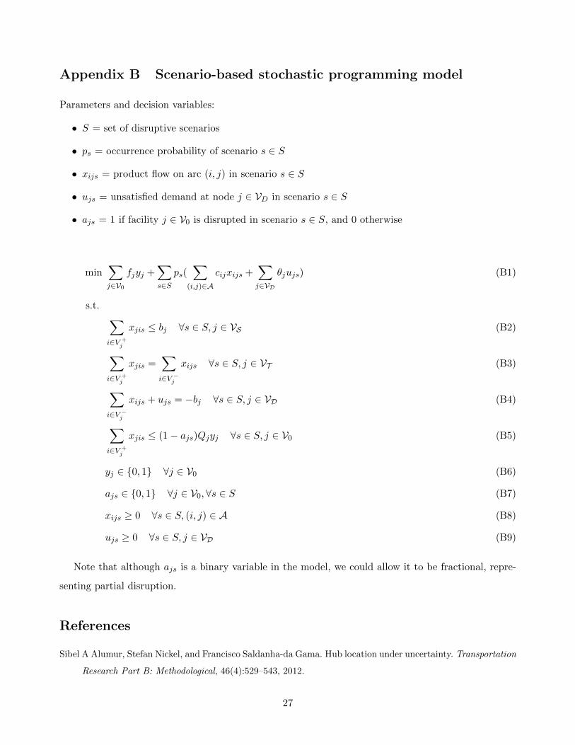
Parameters and decision variables:

• S = set of disruptive scenarios

• ps = occurrence probability of scenario s ∈ S

• xijs = product flow on arc (i, j) in scenario s ∈ S

• ujs = unsatisfied demand at node j ∈ VD in scenario s ∈ S

• ajs = 1 if facility j ∈ V0 is disrupted in scenario s ∈ S, and 0 otherwise

min∑j∈V0

fjyj +∑s∈S

ps(∑

(i,j)∈A

cijxijs +∑j∈VD

θjujs) (B1)

s.t. ∑i∈V +

j

xjis ≤ bj ∀s ∈ S, j ∈ VS (B2)

∑i∈V +

j

xjis =∑i∈V −j

xijs ∀s ∈ S, j ∈ VT (B3)

∑i∈V −j

xijs + ujs = −bj ∀s ∈ S, j ∈ VD (B4)

∑i∈V +

j

xjis ≤ (1− ajs)Qjyj ∀s ∈ S, j ∈ V0 (B5)

yj ∈ {0, 1} ∀j ∈ V0 (B6)

ajs ∈ {0, 1} ∀j ∈ V0, ∀s ∈ S (B7)

xijs ≥ 0 ∀s ∈ S, (i, j) ∈ A (B8)

ujs ≥ 0 ∀s ∈ S, j ∈ VD (B9)

Note that although ajs is a binary variable in the model, we could allow it to be fractional, repre-

senting partial disruption.

References

Sibel A Alumur, Stefan Nickel, and Francisco Saldanha-da Gama. Hub location under uncertainty. Transportation

Research Part B: Methodological, 46(4):529–543, 2012.

27

Yu An and Bo Zeng. Exploring the modeling capacity of two-stage robust optimization: Variants of robust unit

commitment model. IEEE Transactions on Power Systems, 30(1):109–122, 2015.

Yu An, Yu Zhang, and Bo Zeng. The reliable hub-and-spoke design problem: Models and algorithms. Optimiza-

tion Online, 2011.

Yu An, Bo Zeng, Yu Zhang, and Long Zhao. Reliable p-median facility location problem: two-stage robust

models and algorithms. Transportation Research Part B: Methodological, 64:54–72, 2014.

Yu An, Yu Zhang, and Bo Zeng. The reliable hub-and-spoke design problem: Models and algorithms. Trans-

portation Research Part B: Methodological, 77:103–122, 2015.

Alper Atamturk and Muhong Zhang. Two-stage robust network flow and design under demand uncertainty.

Operations Research, 55(4):662–673, 2007.

Nader Azad, Georgios KD Saharidis, Hamid Davoudpour, Hooman Malekly, and Seyed Alireza Yektamaram.

Strategies for protecting supply chain networks against facility and transportation disruptions: an improved

benders decomposition approach. Annals of Operations Research, 210(1):125–163, 2013.

Opher Baron, Joseph Milner, and Hussein Naseraldin. Facility location: A robust optimization approach.

Production and Operations Management, 20(5):772–785, 2011.

Aharon Ben-Tal, Alexander Goryashko, Elana Guslitzer, and Arkadi Nemirovski. Adjustable robust solutions of

uncertain linear programs. Mathematical Programming, 99(2):351–376, 2004.

Dimitris Bertsimas, David B Brown, and Constantine Caramanis. Theory and applications of robust optimiza-

tion. SIAM review, 53(3):464–501, 2011.

Qi Chen, Xiaopeng Li, and Yanfeng Ouyang. Joint inventory-location problem under the risk of probabilistic

facility disruptions. Transportation Research Part B: Methodological, 45(7):991–1003, 2011.

Ivan Contreras, Jean-Francois Cordeau, and Gilbert Laporte. The dynamic uncapacitated hub location problem.

Transportation Science, 45(1):18–32, 2011.

Jean-Francois Cordeau, Federico Pasin, and Marius M Solomon. An integrated model for logistics network

design. Annals of operations research, 144(1):59–82, 2006.

Tingting Cui, Yanfeng Ouyang, and Zuo-Jun Max Shen. Reliable facility location design under the risk of

disruptions. Operations Research, 58(4-part-1):998–1011, 2010.

Zvi Drezner. Heuristic solution methods for two location problems with unreliable facilities. Journal of the

Operational Research Society, 38(6):509–514, 1987.

Maryam Farahani, Hassan Shavandi, and Donya Rahmani. A location-inventory model considering a strategy to

mitigate disruption risk in supply chain by substitutable products. Computers & Industrial Engineering,

108:213–224, 2017.

Virginie Gabrel, Mathieu Lacroix, Cecile Murat, and Nabila Remli. Robust location transportation problems

under uncertain demands. Discrete Applied Mathematics, 164:100–111, 2014.

28

Ruiwei Jiang, Muhong Zhang, Guang Li, and Yongpei Guan. Benders’ decomposition for the two-stage security

constrained robust unit commitment problem. In IIE Annual Conference. Proceedings, page 1. Institute of

Industrial Engineers-Publisher, 2012.

Xiaopeng Li and Yanfeng Ouyang. A continuum approximation approach to reliable facility location design

under correlated probabilistic disruptions. Transportation research part B: methodological, 44(4):535–548,

2010.

Michael Lim, Mark S Daskin, Achal Bassamboo, and Sunil Chopra. A facility reliability problem: formulation,

properties, and algorithm. Naval Research Logistics (NRL), 57(1):58–70, 2010.

M Teresa Melo, Stefan Nickel, and Francisco Saldanha-Da-Gama. Facility location and supply chain

management–a review. European journal of operational research, 196(2):401–412, 2009.

Hokey Min and Gengui Zhou. Supply chain modeling: past, present and future. Computers & industrial

engineering, 43(1):231–249, 2002.

Stefan Miskovic, Zorica Stanimirovic, and Igor Grujicic. Solving the robust two-stage capacitated facility location

problem with uncertain transportation costs. Optimization Letters, 11(6):1169–1184, 2017.

F Parvaresh, SM Moattar Husseini, SA Hashemi Golpayegany, and Behrooz Karimi. Hub network design problem

in the presence of disruptions. Journal of Intelligent Manufacturing, 25(4):755–774, 2014.

Peng Peng, Lawrence V Snyder, Andrew Lim, and Zuli Liu. Reliable logistics networks design with facility

disruptions. Transportation Research Part B: Methodological, 45(8):1190–1211, 2011.

Mir Saman Pishvaee, Reza Zanjirani Farahani, and Wout Dullaert. A memetic algorithm for bi-objective inte-

grated forward/reverse logistics network design. Computers & operations research, 37(6):1100–1112, 2010.

Mir Saman Pishvaee, Masoud Rabbani, and Seyed Ali Torabi. A robust optimization approach to closed-loop

supply chain network design under uncertainty. Applied Mathematical Modelling, 35(2):637–649, 2011.

Xuwei Qin, X Liu, and Lixin Tang. A two-stage stochastic mixed-integer program for the capacitated logistics

fortification planning under accidental disruptions. Computers & Industrial Engineering, 65(4):614–623,

2013.

Farnaz Rayat, MirMohammad Musavi, and Ali Bozorgi-Amiri. Bi-objective reliable location-inventory-routing

problem with partial backordering under disruption risks: A modified amosa approach. Applied Soft

Computing, 59:622–643, 2017.

Shabnam Rezapour, Reza Zanjirani Farahani, and Morteza Pourakbar. Resilient supply chain network design

under competition: A case study. European Journal of Operational Research, 259(3):1017–1035, 2017.

Tadeusz Sawik et al. Supply chain disruption management using stochastic mixed integer programming. Springer,

2018.

Zuo-Jun Max Shen, Roger Lezhou Zhan, and Jiawei Zhang. The reliable facility location problem: Formulations,

heuristics, and approximation algorithms. INFORMS Journal on Computing, 23(3):470–482, 2011.

29

Davood Shishebori, Lawrence V Snyder, and Mohammad Saeed Jabalameli. A reliable budget-constrained fl/nd

problem with unreliable facilities. Networks and Spatial Economics, 14(3-4):549–580, 2014.

Lawrence V Snyder and Mark S Daskin. Reliability models for facility location: the expected failure cost case.

Transportation Science, 39(3):400–416, 2005.

Lawrence V Snyder and Mark S Daskin. Stochastic p-robust location problems. IIE Transactions, 38(11):

971–985, 2006.

Lawrence V Snyder, Maria P Scaparra, Mark S Daskin, and Richard L Church. Planning for disruptions in

supply chain networks. Tutorials in operations research, 2:234–257, 2006.

Lawrence V Snyder, Zumbul Atan, Peng Peng, Ying Rong, Amanda J Schmitt, and Burcu Sinsoysal. Or/ms

models for supply chain disruptions: A review. IIE Transactions, 48(2):89–109, 2016.

Ebrahim Teimuory, F Atoei, Emran Mohammadi, and A Amiri. A multi-objective reliable programming model

for disruption in supply chain. Management Science Letters, 3(5):1467–1478, 2013.

Weijun Xie, Yanfeng Ouyang, and Sze Chun Wong. Reliable location-routing design under probabilistic facility

disruptions. Transportation Science, 50(3):1128–1138, 2015.

Bo Zeng and Long Zhao. Solving two-stage robust optimization problems using a column-and-constraint gener-

ation method. Operations Research Letters, 41(5):457–461, 2013.

Ying Zhang, Mingyao Qi, Wei-Hua Lin, and Lixin Miao. A metaheuristic approach to the reliable location

routing problem under disruptions. Transportation Research Part E: Logistics and Transportation Review,

83:90–110, 2015.

Ying Zhang, Lawrence V Snyder, Mingyao Qi, and Lixin Miao. A heterogeneous reliable location model with

risk pooling under supply disruptions. Transportation Research Part B: Methodological, 83:151–178, 2016.

Long Zhao and Bo Zeng. Robust unit commitment problem with demand response and wind energy. In Power

and Energy Society General Meeting, 2012 IEEE, pages 1–8. IEEE, 2012.

30