Modeling, Identification and Control, Vol. 31, No. 3, 2010, pp. 93–106, ISSN 1890–1328

A Tutorial on Incremental Stability Analysisusing Contraction Theory

J. Jouffroy 1 T.I. Fossen 2 ,3

1Mads Clausen Institute, University of Southern Denmark, DK-6400 Sønderborg, Denmark. E-mail:jerome@mci.sdu.dk

2Department of Engineering Cybernetics, Norwegian University of Science and Technology, N-7491 Trondheim,Norway. E-mail: fossen@ieee.org

3Centre for Ships and Ocean Structures, Norwegian University of Science and Technology, NO-7491 Trondheim,Norway.

Abstract

This paper introduces a methodology for differential nonlinear stability analysis using contraction theory(Lohmiller and Slotine, 1998). The methodology includes four distinct steps: the descriptions of twosystems to be compared (the plant and the observer in the case of observer convergence analysis, the plantand the controller in the case of tracking controller analysis), the definition of an abstract system commonto the two systems and denoted as the “virtual system”, and the convergence study of the virtual systemusing its virtual dynamics representation. The approach is illustrated on several simple examples.

Keywords:Contraction theory, exponential stability, incremental stability, Lyapunov stability, methodology.

Introduction

Stability analysis has long been recognized as a key-stone in the control systems community, and manytechniques have been proposed to check this importantproperty. Among them, Lyapunov theory has becomea central tool of the control community, and Lyapunovfunctions have proven fundamental in stability analy-sis and control design of nonlinear and time-varyingsystems described in the state-space (see for exampleKhalil (1996), Krstic et al. (1995), or Slotine and Li(1991).

One of the main features of Lyapunov-based stabil-ity analysis is the consideration of systems having anequilibrium at the origin of the state-space. In moregeneral cases, such as e.g. trajectory tracking control,the standard methodology consists in making use ofan appropriate change of coordinates to put the sys-

tem under study in the suitable form.

Contraction theory is a more recent tool for ana-lyzing the convergence behavior of nonlinear systemsin state-space form; see Lohmiller and Slotine (1998),Slotine and Wang (2003) and Jouffroy (2003b) for theexplicit incorporation of inputs in the framework ofcontraction. One of the main features of contraction isthat, contrary to traditional Lyapunov-based analysis,it does not require the explicit knowledge of a specificattractor. The stability analysis is performed throughextensive use of virtual displacements, with the systemdynamics being described in a differential framework.

Methodology, i .e. how to apply or use the results ofa theory, is now well-established for Lyapunov func-tions. While it might be tempting to apply directlythese techniques to the world of contraction, a morefruitful approach may be to take into account the speci-ficities of contraction theory to see how it applies on

doi:10.4173/mic.2010.3.2 c© 2010 Norwegian Society of Automatic Control

Modeling, Identification and Control

several concrete examples. The purpose of this paper isto contribute in this important issue, as well as suggestmeans to compare contraction with Lyapunov stabilityanalysis. The present tutorial paper is based on Jouf-froy and Slotine (2004) and Jouffroy (2005).

After this introduction, and in addition to a briefrecall of the main results of contraction theory, weshortly discuss in Section 1 a few simple techni-calities related to the main criterion of contractionwhose Lyapunov counterpart would be the celebratedLyapunov equation. Contraction being also an incre-mental form of stability, i .e. stability of the systemtrajectories with respect to one another (see Angeli(2002), Fromion et al. (1999) and references thereinfor other forms of incremental stability, and Lohmiller(1999), Lohmiller and Slotine (2000b), Lohmiller andSlotine (2000a), Egeland et al. (2001), Aghannanand Rouchon (2003), Jouffroy and Lottin (2002) andJouffroy and Opderbecke (2007) for other applicationsof contraction), Section 2 discusses the importanceof the term “incremental” on the methodologicalpoint-of-view introducing a simple example whosestable behavior can be easily concluded with a simpleLyapunov function. In Section 3, we use the remarksof the previous section to deal more specifically withthe methodological aspects induced by the natureof contraction theory. As expected, these are quitedifferent from those of a traditional stability analysisusing the original Lyapunov theory and ideally, wouldallow to expect contraction to perform as well as inthe Lyapunov case. The approach is illustrated withdifferent simple examples throughout the paper andSection 4 deals specifically with several applicationexamples, namely a robot controller, a ship controllerand the Extended Kalman Filter. Concluding remarksend the paper.

1 Contraction theory

1.1 Contraction analysis

In the following, consider systems described by a non-linear deterministic differential equation in the form

x = f(x, t) (1)

where x is the n-dimensional vector corresponding thestate of the system, t is the time, and f is a nonlinearvector field. In addition, we make the further assump-tion that the system is smooth and that any solutionx(x0, t) initialized in x0 of equation (1) exists and isunique. One of the main features of contraction theoryis to use the concept of virtual displacements of thestate x which, roughly speaking, consists of a slight

modification of the state to see the change it produceson the velocity vector x. The standard notation of avirtual displacement, introduced by Lagrange (Lanc-zos, 1970, p. 38), is δx.

From there, the so-called virtual dynamics are intro-duced by computing the first variation of equation (1),i .e.

δx = δf =∂f

∂x(x, t)δx (2)

If now a state dependent local and virtual change ofcoordinates

δz = Θ(x, t)δx (3)

(where Θ(x, t) is a nonsingular transformation matrix)is performed on expression (2), the virtual dynamicscan be expressed in δz-coordinates as

δz = F (x, t)δz (4)

where the generalized Jacobian F is given by

F =

(Θ + Θ

∂f

∂x

)Θ−1 (5)

We are now ready to state the main definition ofLohmiller and Slotine (1998):

Definition 1 Given the system equations x = f(x, t),a region of the state space is called a contraction re-gion with respect to a uniformly positive definite met-ric M(x, t) = Θ>Θ, if there exists a strictly positiveconstant βM such that

F =

(Θ + Θ

∂f

∂x

)Θ−1 ≤ −βM I (6)

or equivalently

∂f

∂x

T

M + M +M∂f

∂x≤ −2βM M (7)

is verified in that region.

From this definition, Theorem 2 in Lohmiller andSlotine (1998) is stated as:

Theorem 1 Given the system equations x = f(x, t),any trajectory, which starts in a ball of constant radiuswith respect to the metric M(x, t), centered at a giventrajectory and contained at all times in a contractionregion with respect to M(x, t), remains in that ball andconverges exponentially to that trajectory.

Proof. See Lohmiller and Slotine (1998).Intuitively, the above result means that if the tem-

poral evolution of a virtual displacement tends to zeroas time goes to infinity, this being true for all states xand at all time, the whole flow will “shrink” to a point,hence the term “contraction”.

94

J. Jouffroy and T.I. Fossen, “A Tutorial on Incremental Stability Analysis using Contraction Theory”

(a) t = 2s (b) t = 3s (c) t = 4s

(d) t = 5s (e) t = 6s (f) t = 7s

Figure 1: Contracting volume of a nonlinear system

Example 1 To illustrate the above idea, consider thefollowing simulation of a simple three-dimensionalnonlinear system described by the following equation x

yz

=

−0.1 0 00 −0.1 00 0 −0.1− 0.01z2

xyz

+

1 0 00 1 00 0 1

u (8)

where (x, y, z)> is the state. Let u be a time-dependentcontrol input u = (2 sin t, 2 cos t, 5t− 2)>. This systemwas simulated for many different initial conditions ina ball of radius R =

√x20 + y20 + z20 = 10 and centered

about the origin. Figure 1 represents the evolution ofthis ball in time. Since system (8) fulfils the conditionsof the above criterion, the volume contracts in time toa point, as predicted by the theory.

It can actually be shown that the condition of defi-nition 1 and theorem 1 is not only sufficient but neces-sary, as stated in the following converse theorem:

Theorem 2 If the system which equations are x =f(x, t) is exponentially convergent, i .e. its virtual dis-placements verify the following inequality

δx>δx ≤ kδx>0 δx0e−βt

(where δx0 = δx(0) and k and β are strictly positiveconstants) then it is also contracting with respect to auniformly positive definite and initially upper boundedmetric M(x, t).

Proof. See Lohmiller and Slotine (1998, section 3.5).

On the methodological aspect, first note that the as-sumptions that are used on the metric M imply thatit can become unbounded as time goes to infinity. Letus see what simple implication it may have for usingcriteria (6) and (7). Indeed, by looking at the uni-form negative definiteness condition of equation (7),one could think of checking

∂f

∂x

>M + M +M

∂f

∂x≤ −βI (9)

where β is a strictly positive constant. This would

95

Modeling, Identification and Control

obviously imply

d

dt

(δx>Mδx

)≤ −βδx>δx (10)

However, in order to be able to conclude exponentialconvergence, one would like to have

d

dt

(δx>Mδx

)≤ −βMδx>Mδx (11)

with βM a strictly positive constant. Then, note thatthe assumptions on M in Lohmiller and Slotine (1998,Section 3.5) can be expressed as

σ2minδx

>δx ≤ δx>Mδx ≤ σ2max(t)δx>δx (12)

where σmin is a strictly positive constant which standsfor the uniform positive definiteness of M , and σmax(t)is a strictly positive time-dependent function statingthat M is bounded for bounded t, but may be un-bounded as t → +∞. From eq. (10) and eq. (12), wethus get

− βδx>δx ≤ − β

σ2max(t)

δx>Mδx (13)

which in turn implies that

d

dt

(δx>Mδx

)≤ − β

σ2max(t)

δx>Mδx (14)

Using eq. (12) once again, we finally transform eq. (14)into

δx>δx ≤ σ2max(0)

σ2min

δx>0 δx0e−β

∫ t0

1σ2max(τ)

dτ(15)

Hence, because of the form (15), we might not get anexponential convergence if we read eq. (9) for eq. (7).

As a consequence, this latter condition must be readas

∂f

∂x

>M + M +M

∂f

∂x≤ −βMM (16)

which straightforwardly implies

δx>

(∂f

∂x

>M + M +M

∂f

∂x

)δx ≤ −βMδx>Mδx

(17)and therefore

δx>δx ≤ σ2max(0)

σ2min

δx>0 δx0e−βM t (18)

which indicates exponential convergence of the trajec-tories of x = f(x, t).

Note that by using the local transform (3), one canchange eq. (17) into

δz>(F> + F

)δz ≤ −βMδz>δz (19)

hence the equivalence between the negativity conditionon eq. (6) and (7).

Comparing with the usual Lyapunov quadratic func-tions that are used to prove stability of linear (time-varying) systems x = A(t)x, remark that these latterimply the well-known Lyapunov equation

P (t)A(t) +AT (t)P (t) + P (t) = −Q(t) (20)

where it is often assumed that both P (t) and Q(t) areuniformly positive and upper bounded matrices, i.e.

pminI ≤ P (t) ≤ pmaxI (21)

andqminI ≤ Q(t) ≤ qmaxI (22)

While equation (20) together with the boundsabove are very important for computational pur-poses (Gajic and Qureshi, 1995), it does not havethe“proportionality” form of (16) induced by the termβM , leading to the equivalence with (19) which makesit easy to find the transform Θ under which the systemis contracting.

On the other hand, such a proportional inequality aseq. (16) might sometimes be difficult to verify withoutassuming any upper boundedness of the metric M , asit will be seen through an example later in this paper.

Finally, since

d

dt

(δz>δz

)≤ − 2βmax(x, t) δz>δz (23)

where βmax(x, t) is the largest eigenvalue of the sym-metric part of F , note that criterion (6) can be re-laxed to conclude exponential convergence by requir-ing e.g. that the moving-window time-average of Fbe upper bounded, i.e. that for some finite T > 0,∫ t+Tt

λmax(x, τ)dτ be uniformly negative definite intime, as studied in Jouffroy (2003a).

1.2 Partial contraction

In this section we briefly recall the basic principles of anextension of contraction analysis, the so-called partialcontraction analysis. The reader is referred to Slotine(2003) for details.

Theorem 3 Consider a nonlinear system which canbe put under the form

x = f(x, x, t) (24)

and assume that the auxiliary system

y = f(y, x, t) (25)

96

J. Jouffroy and T.I. Fossen, “A Tutorial on Incremental Stability Analysis using Contraction Theory”

is contracting with respect to y. If a particular solu-tion of the auxiliary y-system verifies a smooth specificproperty, then all trajectories of the original x-systemverify this property exponentially. The original systemis said to be partially contracting.

Proof. The virtual, observer-like y-system has twoparticular solutions, namely y(t) = x(t) for all t ≥ 0and the solution with the specific property. This im-plies that x(t) verifies the specific property exponen-tially.

Note that contraction may be trivially regarded asa particular case of partial contraction. Also, considerfor instance an original system in the form

x = c(x, t) + d(x, t) (26)

where function c is contracting in a constant metric.The auxiliary contracting system may then be con-structed as

y = c(y, t) + d(x, t) (27)

and the specific property of interest may consist e.g. ofa relationship between state variables.

2 Incremental and non-incrementalexponential stability

In Jouffroy (2002) and Jouffroy and Slotine (2004) itwas remarked that some particular examples could bequite difficult to analyze at first glance using contrac-tion analysis, whereas their stable behavior was easilyproven with Lyapunov functions, as illustrated in thefollowing example.

Example 2 Consider the system:

d

dt

(xsys

)=

(−1 xs−xs −1

)(xsys

)(28)

This system is very easily proven to be GES (Glob-ally Exponentially Stable) using the Lyapunov func-

tion V = 12 (xs, ys)

>(xs, ys). Note the skew-symmetric

structure that one often encounters e.g. using back-stepping techniques. The stability analysis is easymainly because the cross-terms neutralize each otherin the expression of the time derivative of V . Indeed,V = − (xs, ys)

>(xs, ys) < 0, (xs, ys) 6= (0, 0). Now

using contraction, the virtual dynamics are expressedas

d

dt

(δxsδys

)=

(−1 + ys xs−2xs −1

)(δxsδys

)(29)

Clearly, the skew-symmetric structure is destroyed inthe derivation process leading to the expression of the

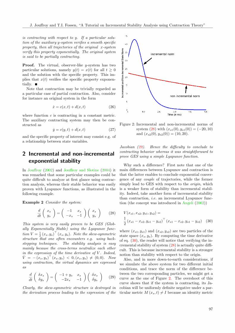
Figure 2: Incremental and non-incremental norms ofsystem (28) with (xs1(0), ys1(0)) = (−20, 10)and (xs2(0), ys2(0)) = (10, 20).

Jacobian (29). Hence the difficulty to conclude tocontracting behavior whereas it was straightforward toprove GES using a simple Lyapunov function.

Why such a difference? First note that one of themain differences between Lyapunov and contraction isthat the latter enables to conclude exponential conver-gence of any couple of trajectories, while the formersimply lead to GES with respect to the origin, whichis a weaker form of stability than incremental stabil-ity. Indeed, take another form of incremental stabilitythan contraction, i.e. an incremental Lyapunov func-tion (the concept was introduced in Angeli (2002))

V (xs1, xs2, ys1, ys2) =

1

2(xs1 − xs2, ys1 − ys2)

>(xs1 − xs2, ys1 − ys2) (30)

where (xs1, ys1) and (xs2, ys2) are two particles of thestate space (xs, ys). By computing the time derivativeof eq. (30), the reader will notice that verifying the in-cremental stability of system (28) is actually quite diffi-cult. This is because incremental stability is a strongernotion than stability with respect to the origin.

Also, and in more down-to-earth considerations, ifwe simulate the above system for two different initialconditions, and trace the norm of the difference be-tween the two corresponding particles, we might get acurve as the one of Figure 2. The overshoot of thiscurve shows that if the system is contracting, its Ja-cobian will be uniformly definite negative under a par-ticular metric M (xs, t) 6= I because an identity metric

97

Modeling, Identification and Control

would correspond to a curve bounded by an exponen-tial whose starting point is the norm of the initial valueof the difference vector (xs1 − xs2, ys1 − ys2).

Hence contraction should therefore be compared toan incremental form of stability. Also, contraction im-plying an exponential form of convergence, the formof incremental stability under study should be expo-nential. As a consequence, let us give the followingincremental version of GES:

Definition 2 The system x = f(x, t) is said to be in-crementally Globally Exponentially Stable (Incremen-tally GES) if there exist two strictly positive constantsk and λ such that the following inequality is verified

‖x(x10, t)− x(x20, t)‖ ≤ k ‖x10 − x20‖ e−λt (31)

(where ‖•‖ is the Euclidian norm) for all x10 and x20in n, all t ≥ 0.

Once incremental GES is defined, the question is howto relate contraction with the former. The followinglemma answers this question.

Lemma 1 Assume that the system

x = f(x, t) (32)

is globally contracting with the contraction rate λ andwith respect to the uniformly positive definite andbounded metric M(x, t), i.e.

σ2minI ≤M(x, t) ≤ σ2

maxI (33)

where σmin and σmax are two strictly positive constants.Then system (32) is also incrementally GES, with i.e.

k =σmax

σmin. (34)

Proof. The first part of the proof is based on Opial(1960) (see also Jouffroy (2005)). Consider a straightline segment s(α) between x10 and x20 defined by

s(α) = αx10 + (1− α)x20, α ∈ [0, 1], (35)

whose length is ‖x10 − x20‖. Consider then the curve”generated” by s(α), defined by x(s(α), t), α ∈ [0, 1].The length L(t) of this curve is given by

L(t) =

∫ α=1

α=0

∥∥∥∥∂x(s(α), t)

∂α

∥∥∥∥ dα. (36)

Defining now v as

v =∂x(s(α), t)

∂α, (37)

it can be seen that v verifies

d

dtv =

∂f(x, t)

∂xv (38)

Then, introducing the local transform Θ(x,t) corre-sponding the metric M(x, t) under which the systemis contracting

w = Θ(x,t)v, (39)

we getd

dtw = F (x,t)w. (40)

Assuming global contraction with rate λ means that Fis uniformly negative definite, and that

w>w ≤ w>0 w0e−2λt (41)

which in turn leads to

v>v ≤ σ2max

σ2min

v>0 v0e−2λt (42)

due to the bounds on M(x, t). Finally, we have

‖v(α, t)‖ ≤ σmax(0)

σmin‖v(α, 0)‖ e−λt (43)

for all α ∈ [0, 1]. After integration on α, we finally have

‖x(x10, t)− x(x20, t)‖ ≤ L(t)

≤ σmax

σmine−λtL(0) =

σmax

σmin‖x10 − x20‖ e−λt (44)

which concludes the proof of the lemma.The other way is even simpler, as can be seen in the

following lemma.

Lemma 2 Assume that the system

x = f(x, t) (45)

is incrementally GES. Then system (45) is also globallycontracting.

Proof. Since eq. (31) is valid for all x1 = x(x10, t)and x2 = x(x20, t), then it is also valid for x1 = x+ δxand x2 = x. Therefore eq. (31) implies

‖δx‖ ≤ k ‖δx0‖ e−λt. (46)

Then, using the converse theorem of the last section,the above inequality implies that (45) is globally con-tracting.

The above lemmas give therefore an equivalence be-tween contraction and incremental exponential stabil-ity. This can be summarized with the following theo-rem:

Theorem 4 The system

x = f(x, t) (47)

is incrementally GES if and only if it is globally con-tracting.Proof. Immediate from Lemma 1 and Lemma 2.

98

J. Jouffroy and T.I. Fossen, “A Tutorial on Incremental Stability Analysis using Contraction Theory”

3 Contraction as a flow-orientedapproach to stability analysis

3.1 Virtual system / actual systems

In order to be able to compare Lyapunov theory withcontraction in terms of applications, one would haveto take into account their differences by requiring theverification of the same stability property. Hence thefollowing question arises: how to prove that system(28) is GES using contraction?

To answer this question, which is the starting pointof the methodology proposed in this paper, let us firstconsider the following elementary generalization.

Example 3 Consider the system

xs = −D(xs)xs (48)

where xs ∈ Rn, D(xs) + D>(xs) ≥ αI > 0. Sincethe time-derivative of the quadratic Lyapunov functionV = 1

2x>s xs is

V = −x>s D(xs)xs ≤ −αx>s xs (49)

the equilibrium point xs = 0 is GES.

To link the above result with contraction theory andincremental stability, let us first go back to the proofof Lemma 1, which implies the definition of a path be-tween two particles x1(t) and x2(t), the state xs(t) ofeq. (48) would represent one end of the path (i.e. forexample x1(t) = xs(t)), while the origin of the state-space would be the other end of the path (x2(t) = 0).In terms of systems and differential equations, it meansthat these two signals are particular solutions of a sin-gle system. However, to one particular solution cancorrespond several different systems, meaning there isgenerally some freedom in choosing the system gener-ating these two solutions. Such a perspective was firstnoticed by Polish mathematician Z. Opial that used avery similar criterion to the one of contraction theory,to then apply it to compare different systems (see thehistorical review Jouffroy (2005)).

This is also the viewpoint that is adopted in Section1.2 to describe partial contraction analysis (Slotine andWang, 2003), where the choice of the so-called auxiliarysystem gives this freedom.

Additionally, note that the definition of a differentialequation is quite abstract and general if no particularinitial value is specified. Specifically, consider a virtualsystem

x = f(x, t) (50)

which can be seen as an auxiliary system in the frame-work of partial contraction. Then, a particular solution

can be specified for example as

xs = x(xs0, t) (51)

in explicit form, or, in implicit form

xs = f(xs, t) (52)

which in the following will be called an actual system.Note that this clear separation of the abstract level ofthe virtual system from the more concrete level of ac-tual systems is also close in spirit to object-orientedprogramming, where classes and objects defined in anabstract way have to be instantiated to be fully mate-rialized.

In the example above, a possible way of defining thevirtual system corresponding to eq. (48) would be thefollowing equation

x = −D(xs)x (53)

which is possible since, if we choose x = xs as a par-ticular solution, we find actual system (48). On theother hand, note that the origin of the state-space isalso a particular solution of (53). This fits well witha methodology for using contraction theory since, ifsystem (53) (and more generally system (50)) is con-tracting, then, as stated by Theorem 1, any couple oftrajectories, and particularly the ones of interest, willconverge to each other.

Coming back to virtual system (53) and calculatingits virtual dynamics

δx = −D(xs)δx (54)

it is easy to conclude to contracting behavior of (53)and hence of exponential convergence of its two par-ticular solutions x = xs and x = 0. This allows us toconclude that system (48) is GES.

Note that if we would have worked directly on eq.(48) using contraction, we would have searched for anincremental form of GES, which is difficult to check, aswe saw in Example 2.

3.2 From observers to controllers

It is worth noting that contraction was first developedin the context of observers; see Lohmiller and Slotine(1996b) for the main principle and Lohmiller and Slo-tine (1996a) for application examples, for which thevirtual system corresponded exactly to the observerequation, as shown by the following example.

Example 4 Define the following observer

˙x = x+ u+ k(xs − x) (55)

99

Modeling, Identification and Control

where k > 1 and u is the control input. The observerestimates the state of the system

xs = xs + u+ k(xs − xs). (56)

Using the virtual system/actual systems description isquite straightforward, since eq. (55) and eq. (56) areparticular systems of the virtual system

x = x+ u+ k(xs − x) (57)

which is contracting.

However, virtual system (57) corresponds exactlyto the observer (55) itself. Indeed, it was noted inLohmiller and Slotine (1998) that for observer conver-gence analysis, one simply had to verify that the systemto be estimated is a particular solution of the observerto ensure that x will converge exponentially to the ac-tual state xs of the system. By duality, it was alsostated that one would have an exponentially conver-gent tracking controller provided that the system tobe controlled is a particular solution of the contractingcontroller. This last statement is true for many con-trollers, in particular for linear static state feedbackcontrollers. But it can be vastly extended using thevirtual system/actual systems description, as seen e.g.in Example 3. Let us discuss this point further throughthe continuation of Example 3 using a control input.

Example 5 Consider the system

xs = −D(xs)xs + u (58)

where xsRn, D(xs) + D>(xs) ≥ αI > 0 and u is thecontrol. Define the controller

xd = −D(xs)xd + u+K(xd)(xs − xd) (59)

where the n-dimensional square matrix K is positivesemi-definite. This controller makes xs and xd con-verge exponentially to one another since the virtual sys-tem

x = −D(xs)x+ u+K(xd)(xs − x) (60)

whose particular solutions x = xs and x = xd are re-spectively syst. (58) and syst. (59), is contracting.

The reader has certainly noticed that the result isquite obvious since the chosen virtual system is actuallylinear. However, note that such controllers as eq. (59)are often used with Lyapunov-based techniques (see forexample Skjetne et al. (2004)), precisely because theymake easier the analysis of the time derivative of theLyapunov function V (x), where x = xs − xd.

This interpretation of partial contraction is of courseuseful for larger classes of systems than eq. (58). Con-sider for instance a nonlinear system of the form

xs = f(xs, xs, xd, u, t) (61)

and assume that the controller equation is such that

xd = f(xd, xs, xd, u, t) (62)

where xd(t) is the desired state. Consider now thevirtual system

x = f(x, xs, xd, u, t) (63)

If the virtual system is contracting, then x tends to xdexponentially, since both are particular solutions of thex-system.

Note that in the analysis of the controller that wascarried out above, controller (62) is represented in animplicit form, contrary to the usual u = c(xs, xd, xd, t)form. In our opinion, it clarifies the reading and thecomparison of system and controller, as well as bringsa unified view of both observers and controllers con-vergence analysis by adopting an observer perspective.This last point can also be related to the concept ofdual observers due to Brasch that are alluded to in Lu-enberger (1971, Section 6) where if an observer couldbe seen as a system S2 tracking another system S1, thecorresponding controller would be S1 that the system-to-be-controlled S2 would have to follow. Finally, notethat this point-of-view also allows to go back and forthbetween observer and controller design, as shown byExample 5 in which we can design a “tricky” but sim-ple observer for system (58) by replacing xd with xin (59) if xs is measured (see also Jouffroy and Lottin(2002) for an application to observer design for Dy-namic Positioning of marine vessels).

Hence, we can summarize the above discussion byintroducing a methodology for controller stability anal-ysis using contraction theory which could be sketchedas follows.

• write the “target” system equation (xs = f(xs, t)),

• write the controller equation in implicit form,

• define the virtual system whose particular solu-tions or actual systems are the target system andthe controller,

• analyze the virtual dynamics of the virtual systemto conclude to contracting behavior.

One might wonder about several types of controllerswhen related to the above methodology, like for exam-ple PID controllers. In this case, the dimension of the

100

J. Jouffroy and T.I. Fossen, “A Tutorial on Incremental Stability Analysis using Contraction Theory”

controller equation can be different from the system un-der consideration, and one has just to make sure thatthe chosen virtual system contains both system andcontroller. Switching again to the observer world, thislast remark can be used to reformulate, in a very sim-ple way, the interesting concept of dynamic observersas introduced by Park et al. (2002).

The problem of analyzing systems synchronizationcan also be studied as in the following example, takenfrom Slotine and Wang (2003).

Example 6 Consider two systems x1 = f (x1, t) andx2 = f (x2, t) coupled in the following manner:

x1 = f (x1, t) + k(x2, t)− k(x1, t)x2 = f (x2, t) + k(x1, t)− k(x2, t)

(64)

where k(xi, t) represent the coupling forces. Assumingthat the virtual system

x = f (x, t)− 2k(x, t) + k(x1, t) + k(x2, t) (65)

is contracting leads to conclude that x1 and x2 convergeexponentially to each other.

3.3 Incorporating input signals

Another question that might arise when using theabove methodology is how to express in an explicitmanner the impact of different inputs on the behav-ior of a system. Hence, we will now have to considersystems described by the following differential equation

x = f (x, u, t) (66)

where x ∈ Rn and u(t) ∈ Rp. From there, the firstvariation of eq. (66) can now be expressed as

δx =∂f

∂x(x, u, t) δx+

∂f

∂u(x, u, t) δu (67)

and the local coordinate transform Θ is now controldependent, i.e.

δz = Θ (x, u, t) δx (68)

and gives the virtual dynamics in the δz-coordinates

δz = Fδz + Θ∂f

∂uδu (69)

where F is the generalized Jacobian (6) except for thedependence on the control input.

From expression (69), it can be seen that providedthat F is uniformly negative definite for all input, thenthe impact of different inputs on the convergent behav-ior will be bounded if ∂f∂u and Θ are uniformly bounded.

Thus, as in the ISS framework of Sontag (1989), expres-sion (69) leads to convergence of a ball around a tra-jectory. As described in Sontag (2000) in the contextof ISS and in Jouffroy (2003b) in the context of con-traction, such a point-of-view helps to consider manydifferent important issues such as robustness, but alsodetectability, combination properties such as cascadesand small-gain theorem in a simple way.

In terms of the above-described methodology, thenotation used in this paper indicates that eq. (66) isthe virtual system whose particular solutions need tobe specified to study incremental stability propertiesof particular examples. However, since we are dealingwith inputs in addition to the state, we will considerthe couple (x = x1, u = u1) and (x = x2, u = u2) as theparticular solutions describing two systems generatedby eq. (66).

Such a point-of-view happens in particular in thecontext of output-feedback where the unavailable statexs of a plant which should be the input to the feedbackcontroller is replaced by its estimate x obtained by anobserver.

The following example shows how to reframe thewell-known separation principle in the context of con-traction for the linear case and a simple nonlinear one.

Example 7 Consider the linear time-invariant system

xs =Axs +Bus (70)

ys =Cxs (71)

where us ∈ Rp and ys ∈ Rq, and A, B and C arematrices of appropriate dimensions. Equations (70)-(71) are assumed to be both controllable and observable.A linear full-state observer for the plant (70)-(71) takesthe form

˙x = Ax+Bus + LC(xs − x) (72)

where the matrix L is the observer gain. A state-feedback controller for (70)-(71) could take the form

xd = Axd +Bus +BK(xs − xd) (73)

Remark first that either (72) or (73) can be used to-gether with (70) to define the following virtual system

x = Ax+Bus + F (xs − x) (74)

where F can be LC or BK, depending on what actionis chosen, i .e. observation or control. Say now thatinstead of controller (73), we want to use the output-feedback controller

xh = Axh +Bus +BK(x− xh) (75)

101

Modeling, Identification and Control

whose input is the estimate x given by observer (72).Then, the difference in terms of behavior with con-troller (73) can be seen by writing the following virtualsystem

xc = Axc +Bus +BK(xo − xc) (76)

where the particular solutions (xc = xd, xo = xs) and(xc = xh, xo = x) are respectively eq. (73) and eq.(75), and where xo is in turn the state of the virtualsystem

xo = Axo +Bus + LC(xs − xo) (77)

obtained from the actual systems defined by plant (70)and observer (72). Finally, putting together the virtualdynamics of virtual systems (76) and (77), we have

d

dt

(δxoδxc

)=

(A− LC 0BK A−BK

)(δxoδxc

)(78)

which is contracting provided that each element of thecascade (observer and controller parts) is contractingand that BK is bounded.

Example 8 Take now, as in Lohmiller and Slotine(2000b), the following nonlinear closed-loop system

zs = f(zs, t) +G(zs, t)u(z, t) (79)

with its corresponding observer

˙z = f(z, t) +G(zs, t)u(z, t) + e(zs, t)− e(z, t) (80)

and define the virtual observer system

zo = f(zo, t) +G(zs, t)u(z, t) + e(zs, t)− e(zo, t) (81)

Like the linear system, define also the virtual controllersystem

zc = f(zc, t) +G(zc, t)u(zo, t) (82)

which, together with eq. (81) give the virtual dynamics

d

dt

(δzoδzc

)=

(∂(f−e)∂zo

0

G ∂u∂zo

∂(f+Gu)∂zc

)(δzoδzc

)(83)

which is again contracting provided ∂(f−e)∂zo

and ∂(f+Gu)∂zc

are uniformly negative definite and G ∂u∂zo

is uniformlybounded.

4 Applications

4.1 Robot manipulator control design

Consider the nonlinear robot model Asada and Slotine(1986):

qs = vs (84)

H(qs)vs + C(qs, vs)vs + g(qs) = τ (85)

where qs ∈ Rn is a vector of joint angles, H(qs) =H>(qs)>0 is the inertia matrix, the matrix C(qs, vs)defines Coriolis and centripetal terms, g(qs) is a vectorof gravitational torques, and τ ∈ Rn is a vector ofcontrol torques. Using a control design technique suchas vectorial backstepping gives, for system (84)-(85),the following nonlinear controller (see Fossen (2002))

τ = H(qs)vr +C(qs, vs)vr + g(qs)−Kds−Kq(qs− qd),(86)

where qd is a smooth desired trajectory, vd = qd,and Kd and Kq are strictly positive constant matrices.Variable s is defined as s = (vs−vd)+Λ(qs−qd), with Λis a constant Hurwitz matrix, while vr = qd−Λ(qs−qd).Controller (86) can easily be rewritten as

H(qs)vd + C(qs, vs)qd + g(qs) = τ

+ [C(qs, vs)Λ +KdΛ +Kq](qs − qd)+ [H(qs)Λ +Kd](vs − vd) (87)

By comparing this controller with robot model (85),one can now write the virtual system equation

H(qs)v + C(qs, vs)q + g(qs) = τ

+ [C(qs, vs)Λ +KdΛ +Kq](qs − q)+ [H(qs)Λ +Kd](vs − v) (88)

and compute its virtual dynamics

Hδv + Cδq = −[CΛ +KdΛ +Kq]δq

−[HΛ +Kd]δv (89)

which, in matrix form, gives(I 00 H

)(δqδv

)=(

0 I−[CΛ +KdΛ +Kq] −[HΛ + C +Kd]

)(δqδv

)(90)

Introducing now the local transform(δqδs

)=

(I 0Λ I

)(δqδv

)(91)

gives the generalized Jacobian dynamics(δqδs

)=

(−Λ I

−H−1Kq −H−1(C +Kd)

)(δqδs

)(92)

Then, we use yet another change of local coordinatesinduced by the metric

M =

(Kq 00 H

)(93)

102

J. Jouffroy and T.I. Fossen, “A Tutorial on Incremental Stability Analysis using Contraction Theory”

to check the quadratic criterion of contraction on eq.(92), i.e.

d

dt

((δq> δs>

)( Kq 00 H

)(δqδs

))= −2

(δq> δs>

)( KqΛ −Kq

Kq Kd

)(δqδs

)= −2

(δq> δs>

)( KqΛ 00 Kd

)(δqδs

)(94)

leading to contracting behavior of system (88).From the above computations, one can notice that

we have introduced two different changes of coordinatesinto two different forms, namely a local transform Θand a metric M . Interestingly, one can see that Θis induced by the virtual control law process of thebackstepping procedure, or of the sliding variable s,while the metric M is the counterpart of the quadraticLyapunov function that is typically used for such aproblem.

Alternatively, consider the energy-based controllerSlotine and Li (1991)

H(qs)vr + C(qs, vs)vr + g(qs)−K(vs − vr) = τ (95)

with K a constant s.p.d. matrix. The virtual x-system

H(qs)v + C(qs, vs)v + g(qs)−K(vs − v) = τ (96)

has vs and vr as particular solutions, and furthermoreis contracting, since the skew-symmetry of the matrixH − 2C implies

d

dtδv>Hδv = −2δv>(C+K)δv+δv>Hδv = −2δv>Kδv

(97)Thus vs tends to vr exponentially. Making then theusual choice vr = vd − Λ(qs − qd), where Λ a constantHurwitz matrix, implies in turn that qs tends to qdexponentially.

4.2 Ship maneuvering control design

In Fossen (2002), a MIMO nonlinear backsteppingtechnique for ship maneuvering is presented. Con-sider a marine vessel moving in the horizontal planedescribed by the following model class:

ηs = R(ψs)νs

Hνs + C(νs)νs +D(νs)νs + g(ηs) = τ

where ηs = (xs, ys, ψs)> is the vector of earth-

fixed coordinates and yaw angle of the ship, νs =(us, vs, rs = ψs)

> represent the body-fixed coordinates(surge, sway, yaw). H is the inertia matrix includ-ing hydrodynamics and added mass, C is the coriolisand centripetal matrix, D the linear and nonlinear dis-sipative terms, and g the vector of gravitational andbuoyancy forces and moments. τ is the vector of con-trol forces and moments. The rotation matrix in yawis written as

R(ψs) =

cos(ψs) − sin(ψs) 0sin(ψs) cos(ψs) 0

0 0 1

(98)

The different quantities are defined in Fossen (2002).Assume that the reference trajectory given by

η(3)d , ηd, ηd, and ηd is smooth and bounded. Using vec-

torial backstepping and similarly to section 4.1, thenonlinear ship controller from Fossen (2002) can be de-scribed as

ηd = R(ψs)νd

Hνd + C(νs)νd +D(νs)νd + g(ηs) = τ

+ [HR>Λ +R>Kd]R(νs − νd)+ [HR>Λ + (C +D)R>Λ

+R>(Kp +KdΛ)](ηs − ηd) (99)

where Λ is a constant Hurwitz matrix, Kd and Kp arestrictly positive constant matrix of the feedback partof the nonlinear PD-controller.

From there, and as in the previous subsection, onecan define the following virtual system

η = R(ψs)ν

Hν + C(νs)ν +D(νs)ν + g(ηs) = τ

+ [HR>Λ +R>Kd]R(νs − ν)

+ [HR>Λ + (C +D)R>Λ

+R>(Kp +KdΛ)](ηs − η) (100)

whose virtual dynamics can be put into matrix form(102), which can be shown to be contracting after theuse of the local transform(

δηδs

)=

(I 0Λ R

)(δηδν

)(101)

(I 00 H

)(δηδν

)=

(0 R

−[HR>Λ + (C +D)R>Λ +R> (KdΛ +Kq)] −[HR>ΛR+ (C +D) +R>KdR]

)(δηδν

)(102)

103

Modeling, Identification and Control

and the metric

M =

(Kp 00 RHR>

)(103)

giving indeed

d

dt

((δη> δs>

)( Kp 00 RHR>

)(δηδs

))= −2

(δη> δs>

)( KpΛ 00 RHR> +Kd

)(δηδs

).

4.3 Extended Kalman Filtering

Despite extensive use of the celebrated ExtendedKalman Filter (EKF) for many practical applications,its proof of convergence as an observer has been ad-dressed only recently, using mainly the frameworkof the second method of Lyapunov in the determin-istic case; see for example Reif et al. (1998), forthe continuous-time case and Boutayeb and Darouach(1997) for the discrete-time case, as well as referencestherein. We present, under specific assumptions, a sim-ple proof of exponential convergence of the EKF basedon contraction theory.

Consider a plant represented by the following non-linear equations

xs =f(xs, t) (104)

ys =h(xs, t) (105)

where xs ∈ Rn is the state of the system to be esti-mated, ys ∈ Rm is the measured output, and wheref and h are smooth vector fields. The EKF observerstructure is

˙x = f(x, t) +K(x, t) [y − h(x, t)] (106)

where the gain matrix

K(x, t) = P (t)C(x, t)>R−1 (107)

is computed using the Riccati matrix differential equa-tion

P (t) = A(x, t)P (t) + P (t)A>(x, t) +Q

− P (t)C>(x, t)R−1C(x, t)P (t) (108)

where

A(x, t) =∂f(x, t)

∂x

∣∣∣∣x=x

, C(x, t) =∂h(x, t)

∂x

∣∣∣∣x=x(109)

The covariance matrices Q = Q> > 0 and R = R> > 0for simplicity are assumed to be constant.

We make the highly non-trivial but standard follow-ing assumption (Reif et al., 1998).

Assumption 1 The P matrix of the Riccati equation(108) is uniformly positive definite and upper bounded,i .e. there exist two strictly positive constants pmin andpmax such that

pminI ≤ P (t) ≤ pmaxI (110)

Taking into account the definitions as well as the as-sumptions for the EKF described above in (104)-(110),we are ready to state the following result.

Theorem 5 Under Assumption 1, the estimate x ofthe EKF converges exponentially to the actual state xsof the system xs = f(xs, t).Proof. The proof starts by using the methodologydescribed in the previous section. Indeed, examining(104) and (106), we can define the following virtualsystem:

x = f (x, t) +K(x, t) [ys − h(x, t)] (111)

which particular solution x = xs gives the state equa-tion of the plant (104), while the other particular so-lution x = x gives observer equation (106). It remainsto prove that syst. (111) is contracting. K and ys areexternal functions of time, so that its virtual dynamicscan be written

δx = (A−KC)δx (112)

Consider now the square length defined by the metricM = P−1

δz>δz = δx>P−1δx (113)

and compute its time-derivative as

d

dt(δx>P−1δx)

= δx>P−1δx+δx>d

dtP−1δx+δx>P−1δx

= δx>[(A−KC)>P−1 +d

dtP−1 + P−1(A−KC)]δx

= δx>P−1[P (A−KC)> − P + (A−KC)P

]P−1δx

(114)

using the fact that ddtP

−1 = −P−1PP−1. Using Ric-cati matrix differential equation (108) and the defini-tion of gain matrix (107), this gives

d

dt(δx>P−1δx) = −δx>C>R−1Cδx−δx>P−1QP−1δx

(115)Since R = R> > 0, using the coordinate transformδy = Cδx on the first term of the right hand side fur-ther implies

d

dt(δx>P−1δx) ≤ −δx>P−1QP−1δx (116)

104

J. Jouffroy and T.I. Fossen, “A Tutorial on Incremental Stability Analysis using Contraction Theory”

Under Assumption 1 and using the lower bound qmin

on Q, this in turn implies

d

dt(δx>P−1δx) ≤ − qmin

pmaxδx>P−1δx (117)

which shows that virtual system (111) is contracting.Hence the estimate x converges exponentially to the ac-tual state xs.

Note the similarity of the proof with that of the con-tinuous Kalman filter for linear systems. This is dueto the differential framework in which contraction the-ory is defined, as well as the appropriate definition ofthe virtual system for the stability analysis using con-traction which would have been much more difficultworking directly on actual system (106). Additionally,following the discussion at the end of Section 1.1, notethat the EKF proof requires an upper bounded metricM = P−1 to allow conclusion of exponential conver-gence.

5 Concluding remarks

By taking advantage of the way contraction theory isdefined, we have presented a methodology for incre-mental stability analysis which depart quite far fromthe one that is usually applied in the context of Lya-punov theory. One of its main features is to considertwo different levels of system description, namely thevirtual system, which can be seen as an abstract def-inition of a differential equation since no initial valueor particular solution is specified, and the actual sys-tems or particular solutions that are the result of aninstanciation of the above virtual system.

The other important feature, which is another fun-damental aspect of contraction theory, is the extensiveuse of virtual displacements that help to eliminate ina rigorous and efficient way the terms that are not di-rectly responsible for the convergent behavior of thesystem. This variational approach was seen to be quiteeffective at simplifying computations in a variety ofcases.

Using this methodology, it seems that it could be ap-pealing for both linear and nonlinear designs. Indeed,it makes appear in an explicit way different kinds oflinearities hidden behind an observer or a controllerdesign, whether these linearities come from a pure lin-ear system, a state-affine representation, or a Lipschitzcondition.

References

Aghannan, N. and Rouchon, P. An intrisic observerfor a class of Lagrangian systems. IEEE Transac-

tions on Automatic Control, 2003. 48(6):936–945.doi:10.1109/TAC.2003.812778.

Angeli, D. A Lyapunov approach to incremental sta-bility properties. IEEE Transactions on AutomaticControl, 2002. 47(3):410–421. doi:10.1109/9.989067.

Asada, H. and Slotine, J.-J. E. Robot Analysis andControl. Wiley-Interscience, 1986.

Boutayeb, H. R., M. and Darouach, M. Convergenceanalysis of the Extended Kalman Filter used asan observer for nonlinear deterministic discrete-timesystems. IEEE Transactions on Automatic Control,1997. 42(4):581–586. doi:10.1109/9.566674.

Egeland, O., Kristiansen, E., and Nguyen, T.-D. Observer for Euler-Bernouilli beam with hy-draulic drive. In Proc. IEEE Conf. on Deci-sion and Control. Orlando, Florida, USA, 2001.doi:10.1109/.2001.980864.

Fossen, T. I. Marine Control Systems: Guidance, Nav-igation and Control of Ships, Rigs and Underwatervehicles. Marine Cybernetics, 2002.

Fromion, V., Scorletti, G., and Ferreres,G. Nonlinear performance of a PI con-trolled missile: an explanation. InternationalJournal of Robust and Nonlinear Control,1999. 9(8):485–518. doi:10.1002/(SICI)1099-1239(19990715)9:8¡485::AID-RNC417¿3.0.CO;2-4.

Gajic, Z. and Qureshi, M. T. J. Lyapunov matrix equa-tion in system stability and control. Academic Press,1995.

Jouffroy, J. Stability and nonlinear systems: reflectionson contraction analysis (in French). Ph.D. thesis,Universite de Savoie, Annecy, France, 2002.

Jouffroy, J. A relaxed criterion for contraction theory:application to an underwater vehicle observer. In Eu-ropean Control Conference. Cambridge, UK, 2003a.

Jouffroy, J. A simple extension of contraction theory tostudy incremental stability properties. In EuropeanControl Conference. Cambridge, UK, 2003b.

Jouffroy, J. Some ancestors of contractionanalysis. In Proc. Conference on Deci-sion and Control 2005. Sevilla, Spain, 2005.doi:10.1109/CDC.2005.1583029.

Jouffroy, J. and Lottin, J. On the use of contrac-tion theory for the design of nonlinear observers forocean vehicles. In Proc. American Control Con-ference 2002. Anchorage, Alaska, pages 2647–2652,2002. doi:10.1109/ACC.2002.1025186.

105

Modeling, Identification and Control

Jouffroy, J. and Opderbecke, J. Underwater navigationusing diffusion-based trajectory observers. IEEEJournal of Oceanic Engineering, 2007. 32(2):313–326. doi:10.1109/JOE.2006.880392.

Jouffroy, J. and Slotine, J.-J. E. Methodological re-marks on contraction theory. In Proc. Conferenceon Decision and Control 2004. Paradise Island, Ba-hamas, 2004. doi:10.1109/CDC.2004.1428824.

Khalil, H. Nonlinear systems (2nd ed.). Prentice-Hall,New-York, 1996.

Krstic, M., Kanellakopoulos, I., and Kokotovic, P.Nonlinear and adaptive control design. Wiley Inter-science, New-York, 1995.

Lanczos, C. The variational principles of mechanics(4th ed.). Dover, New-York, 1970.

Lohmiller, W. Contraction analysis for nonlinear sys-tems. Ph.D. thesis, Dep. Mechanical Eng., M.I.T.,Cambridge, Massachusetts, 1999.

Lohmiller, W. and Slotine, J.-J. E. Applications ofmetric observers for nonlinear systems. In IEEE Int.Conf. on Control Applications. Dearborn, Michigan,1996a. doi:10.1109/CCA.1996.558805.

Lohmiller, W. and Slotine, J.-J. E. On metric ob-servers for nonlinear systems. In IEEE Int. Conf. onControl Applications. Dearborn, Michigan, 1996b.doi:10.1109/CCA.1996.558742.

Lohmiller, W. and Slotine, J.-J. E. On contractionanalysis for nonlinear systems. Automatica, 1998.34(6):683–696. doi:10.1016/S0005-1098(98)00019-3.

Lohmiller, W. and Slotine, J.-J. E. Control system de-sign for mechanical systems using contraction theory.IEEE Transactions on Automatic Control, 2000a.45(5):984–989. doi:10.1109/9.855568.

Lohmiller, W. and Slotine, J.-J. E. Nonlinear processcontrol using contraction theory. A.I.Ch.E. Journal,2000b. 46(3):588–596.

Luenberger, D. G. An introduction to observers.IEEE Transactions on Automatic Control, 1971.16(6):596–602. doi:10.1109/TAC.1971.1099826.

Opial, Z. Sur la stabilite asymptotique des solu-tions d’un systeme d’equations differentielles. Ann.Polonici Math., 1960. 7:259–267.

Park, J.-K., Shin, D.-R., and Chung, T. M. Dynamicobservers for linear time-invariant systems. Auto-matica, 2002. 38:1083–1087. doi:10.1016/S0005-1098(01)00293-X.

Reif, K., Sonnemann, F., and Unbehauen, R. An EKF-based nonlinear observer with a prescribed degreeof stability. Automatica, 1998. 34(9):1119–1123.doi:10.1016/S0005-1098(98)00053-3.

Skjetne, R., Fossen, T. I., and Kokotovic, P. Ro-bust output maneuvering for a class of nonlin-ear systems. Automatica, 2004. 40(3):373–383.doi:10.1016/j.automatica.2003.10.010.

Slotine, J.-J. E. Modularity stability tools for dis-tributed computation and control. Int. Journalof Adaptive Control and Signal Processing, 2003.17(6):397–416. doi:10.1002/acs.754.

Slotine, J.-J. E. and Li, W. Applied nonlinear control.Prentice Hall, Englewood Cliffs, New Jersey, 1991.

Slotine, J.-J. E. and Wang, W. A study of synchroniza-tion and group cooperation using partial contractiontheory. In K. V., editor, Block Island Workshop onCooperative Control. Springer-Verlag, 2003.

Sontag, E. D. Smooth stabilization implies coprime fac-torization. IEEE Transactions on Automatic Con-trol, 1989. 34:435–443. doi:10.1109/9.28018.

Sontag, E. D. The ISS philosophy as a unifying frame-work for stability-like behavior. In Nonlinear Controlin the Year 2000 (Vol. 2), pages 443–448. Springer-Verlag, 2000. doi:10.1007/BFb0110320.

106