a total lagrangian finite element analysis for metal
TRANSCRIPT

Louisiana State UniversityLSU Digital Commons
LSU Historical Dissertations and Theses Graduate School
1989
A Total Lagrangian Finite Element Analysis forMetal Forming With Application to MetalExtrusion.Mehrdad ForoozeshLouisiana State University and Agricultural & Mechanical College
Follow this and additional works at: https://digitalcommons.lsu.edu/gradschool_disstheses
This Dissertation is brought to you for free and open access by the Graduate School at LSU Digital Commons. It has been accepted for inclusion inLSU Historical Dissertations and Theses by an authorized administrator of LSU Digital Commons. For more information, please [email protected].
Recommended CitationForoozesh, Mehrdad, "A Total Lagrangian Finite Element Analysis for Metal Forming With Application to Metal Extrusion." (1989).LSU Historical Dissertations and Theses. 4843.https://digitalcommons.lsu.edu/gradschool_disstheses/4843

INFORMATION TO USERS
The most advanced technology has been used to photograph and reproduce this manuscript from the microfilm master. UMI films the text directly from the original or copy submitted. Thus, some thesis and dissertation copies are in typewriter face, while others may be from any type of computer printer.
The quality of this reproduction is dependent upon the quality of the copy submitted. Broken or indistinct print, colored or poor quality illustrations and photographs, print bleedthrough, substandard margins, and improper alignment can adversely affect reproduction.
In the unlikely event that the author did not send UMI a complete manuscript and there are missing pages, these will be noted. Also, if unauthorized copyright material had to be removed, a note will indicate the deletion.
Oversize materials (e.g., maps, drawings, charts) are reproduced by sectioning the original, beginning at the upper left-hand corner and continuing from left to right in equal sections with small overlaps. Each original is also photographed in one exposure and is included in reduced form at the back of the book. These are also available as one exposure on a standard 35mm slide or as a 17" x 23" black and white photographic print for an additional charge.
Photographs included in the original manuscript have been reproduced xerographically in this copy. Higher quality 6" x 9" black and white photographic prints are available for any photographs or illustrations appearing in this copy for an additional charge. Contact UMI directly to order.
University Microfilms International A Bell & Howell Information C om pany
3 0 0 North Z eeb R oad, Ann Arbor, Ml 4 8 1 06 -1346 USA 3 1 3 /7 6 1 -4 7 0 0 8 0 0 /5 2 1 -0 6 0 0

Order N um ber 0025304
A T o ta l L a g ra n g ia n U nite e le m e n t a n a ly s is fo r m e ta l fo rm in g w i th a p p lic a t io n to m e ta l e x tru s io n
Foroozesh, M ehrdad, Ph.D .
The Louisiana State University and Agricultural and Mechanical Col., 1989
U M I300 N. Zeeb Rd.Ann Arbor, MI 48106

A T o t a l L i i g r a n g i a n F in i t e ’ E l e m e n t A n a l y s i s for M e t a ! F o r m i n g w i t h
A p p l i c a t i o n t o M e t a l E x t e n s i o n
A D i s s e r t a t i o n
S u b m i t ter! t o t h e G r a d u a t e F a c i l i t y o f t h e L o u i s i a n a S t a t e U n i v e r s i t y a n d
A g r i c u l t u r a l a n d M e c h a n i c a l C o l l e g e in p a r t i a l f u l f i l lm e n t o f t h e
r e q u i r e m e n t s for t h e d e g r e e o f D o c t o r o f P h i l o s o p h y
in
T h e D e p a r t m e n t o f C iv i l E n g i n e e r i n g
byM e h r d a d F0 r0 0 7 . e s h
U . S . , L o u i s i a n a S t a t e U n i v e r s i t y , 1 0 8 3
M . S . , L o u i s i a n a S t a t e U n i v e r s i t y , 1 9 8 8
December 1989

A C K N O W L E D G M E N T S
Many people have earned my gratitude during the course of this study. I
specifically wish to thank my parents for the encouragement, moral support, and
the financial support that they have given me which has helped me to advance
this far and to achieve goals which would have been impossible for me to achieve
without their constant guidance. I thank my wife, Mehri, for her understanding
and support. Her presence by my side has been a valuable asset. I dedicate this
work to her and my son, Paymon. I thank my sisters Maryam and Mahtab for
encouraging me to continue my education.
I express my sincere appreciation to Dr. George Z. Voyiadjis who has guided
me through the graduate school and who has provided me with a research assis-
tantship for the final year of my graduate studies. His aid and knowledge has
made this work possible. To Dr. Richard R. Avent, Dr. Mehmet T. Tumay, Dr.
Fariborz Barzegar, Dr. Flora Wang, and Dr. M. Sabbaghian, I express my true
appreciation for the valuable advice that they have given me and for serving as
members of my advisory committee.
I wish to express my gratitude to the members of the Department of Civil
Engineering at LSU and in particular to the chairman of the department, Professor
Roger K. Seals, who provided me with financial assistance during the first four
years of my graduate studies. I also wish to express my appreciation to the College
of Engineering for providing some of the computer time needed to perform the
analyses required to complete this study.
Partial support of this research was provided by the National Science Foun
dation under grant No. MSM-8800832.

T A B L E O F C O N T E N T S
Page
ACKNOW LEDGM ENTS...................................................................................................ii
LIST OF FIG U R E S.............................................................................................................v
LIST OF TA BLES.............................................................................................................vii
A B S T R A C T ...................................................................................................................... viii
1. IN TRO D U CTIO N ...........................................................................................................1
1.1 General R em arks................................................................................................... 1
1.2 Objectives................................................................................................................ 5
1.3 S cope......................................................................................................... 6
2. FIN ITE ELEM ENT FORM ULATION..................................................................... 9
2.1 In troduction ............................................................................................................ 9
2.2 M athematical Form ulations................................................................ 10
3. MATERIAL MODEL AND ITS IM PLEM ENTATION......................................15
3.1 In tro d u ctio n ..........................................................................................................15
3.2 Prelim inary Definitions and Relations............................................................17
3.3 Constitutive Model for Elasto-Plastic Behavior of M etals ......................23
3.4 Numerical Implementation of the M aterial M odel......................................31
3.5 A Simple Vectorization Technique ..............................................................41
3.6 Uniaxial Verification of the Material M odel.................................................44
4. SIMULATION OF CONTACT BOUNDARIES...................................................49
4.1 In tro d u ctio n ......................................................................................................... 49
4.2 Hermite Formulation of Cubic Curves..................................... 50
4.3 Motion of the Nodal Points on the Curved Boundaries ...................... 54
4.4 Use of Multiple Curves in Generating Complex B oundaries....................57
4.5 Description of the Relevant Subroutines.......................................................60
iii

Page
5. PARAMETRIC STUDY OF AXISYMMETRIC EXTRUSION....................... 62
5.1 In troduction .....................................................................................................62
5.2 Comparison of Different Element Types and M eshes................................ 66
5.3 Numerical Results Obtained Using Run A 5 ................... 75
5.4 Study of Various Area Reduction and Die Angle Changes........................85
6. UNIFES USERS G U ID E..........................................................................................96
6.1 In troduction .............. 96
6.2 Input Commands.............................................................................................. 97
7. CONCLUSIONS........................................................................................................112
REFEREN CES..............................................................................................................114
APPENDICES
A. UNIFES............................................................................................................. 121
B. Solver M odule...................................................................................................172
C. Plasticity M odule............................................................................................. 176
D. Contact Boundary Simulation M odule................... 196
E. Elasticity M odule....................................................... 206
F. Element Library Module ...................................................................... 210
G. I/O M odule...................................................................................................... 228
H. Real I/O Utilities Module...................................................................... 248
I. Virtual I/O Utilities M odule...........................................................................251
J. Initializer M odule............................................................................................. 255
K. Graphics M odule............................................................................................. 256
L. Block Data M odule..........................................................................................280
V ITA ................................................................................................................................ 282
iv

LIST OF FIGURES
Page
3.1 Coordinate Systems and Description of Displacement..............................19
3.2 Modification of Prager’s Kinematic HardeningRule by Shield and Ziegler [1958]................................................................ 27
3.3 Experimental and Numerical Stress-Strain Diagramsfor a Uniaxial Problem .................................................................................. 45
4.1 Hermite Parametric Cubic C urve................................................................. 52
4.2 Some Possible Shapes of the Hermite Curve...............................................52
4.3 Correction Process for the Motion of the PointsConstrained to Move on the D ie................................................................ .55
4.4 Illustration of what Necessitates Zoning of theHermite Splines............................................................................................... 59
5.1 Schematic Representation of the Die and the Initial Positionof the B illet........................... 64
5.2 Meshes Used for Runs Al Through A5........................................................68
5.3 Extrusion Pressure Versus Displacement for Run A2(Incomplete Extrusion).................................................................................. 70
5.4 Extrusion Pressure Versus Displacement for Run A 3 .............................. 71
5.5 Extrusion Pressure Versus Displacement for Run A 4 .............................. 72
5.6 Extrusion Pressure Versus Displacement for Run A 5 .............................. 74
5.7 The Yield Zone at Various Stages of the Extrusionfor Run A5........................................................................................................76
5.8 Radial Stress Distribution for Run A 5........................................................ 77
5.9 Axial Stress Distribution for Run A 5 .......................................................... 78
5.10 Shear Stress Distribution for Run A 5 .......................................................... 79
5.11 Circumferential Stress Distribution for Run A 5 ........................................ 80
5.12 Cauchy Volumetric Stress Distribution for Run A 5........................... .81
5.13 Radial and Axial Strain Distributions for Run A5.................................... 82
v

Page
5.14 Shear and Circumferential Strain Distribution for Run A 5 ..................... 83
5.15 Distribution of the Plastic Work Intensity for Run A5............................ 84
5.16 Extrusion Pressure Versus Displacement for RunsB l, B2, and B3........................................................................... 89
5.17 Extrusion Pressure Versus Displacement forRuns C l, C2, and C 3..................................................................................... .90
5.18 Extrusion Pressure Versus Displacement forRuns D l, D2, and D3 .............................................. 91
5.19 Steady-State Extrusion Pressure Versus theVariation in the Die Angle............................... 92
5.20 Peak Extrusion Pressure Versus theVariation in the Die Angle.................. 93
5.21 Steady-State Extrusion Pressure Versusthe % Reduction in A rea ........................ 94
5.22 Peak Extrusion Pressure Versusthe % Reduction in A rea ..................................................................................95
6.1 Sequence of Node Numbers and Identification Codesfor 2D Quadrilateral E lem ents.................................................... 99
6.1 Sequence of Node Numbers and Identification Codesfor 3D Solid E lem ents..................................................................................... 100
vi

LIST OF TABLES
PaSe3.1 Sequence of Computations Required for the First Stage of
Implementation (Evaluation of the D M atrix).......................................... 34
3.2 Sequence of Computations Required for the Second Stage ofImplementation (Evaluation of the Stresses, e tc .) .................................... 36
3.3 Input File for the Uniaxial Test (First Loading)........................................46
3.4 Input File for the Uniaxial Test (Second Loading)....................................47
3.5 Input File for the Uniaxial Test (Third Loading)...................................... 48
5.1 Material Parameters for Aluminum 2024-T4..............................................62
5.2 Parameters Used for the Control of the Iterative SolutionProcess........................................................................... 65
5.3 Mesh Characteristics for Runs A1 Through A5..........................................66
5.4 Parameters Used to Generate the Die for Runs A1 Through A5Using the Hermite Formulation.................................................................... 67
5.5 Identification Codes for Each Analysis........................................................ 86
5.6 Parameters Used to Generate the Die for Run B l ....................................87
5.7 Parameters Used to Generate the Die for Run B 2....................................87
5.8 Parameters Used to Generate the Die for Run B 3....................................87
5.9 Parameters Used to Generate the Die for Run C l ....................................87
5.10 Parameters Used to Generate the Die for Run C 2................................... 87
5.11 Parameters Used to Generate the Die for Run C 3................................... 88
5.12 Parameters Used to Generate the Die for Run D 1................................... 88
5.13 Parameters Used to Generate the Die for Run D 2........................... 88
5.14 Parameters Used to Generate the Die for Run D 3................................... 88
vii

A B S T R A C T
A detailed formulation for finite element analysis of metal forming problems
is carried out in this work. It incorporates every aspect of the analysis, including
the iterative solution procedures for geometric and material non-linearities, imple
m entation of the m aterial model, and formulation of curved contact boundaries.
The finite element formulation is based on a Total Lagrangian approach which
by-passes the use of the Jaum ann stress rate tensor commonly used in the Up
dated Lagrangian formulation. The yield model used is of the von Mises type with
both kinematic and isotropic hardening and is formulated in the Eulerian space.
This model is then transformed to the Lagrangian reference frame. In the evalu
ation of stresses, yielding is first, detected through the use of an elastic-predictor
stress; subsequently upon detection of yielding, the consistency condition is used
to evaluate the actual stress and plastic strain tensors. This method is used in
conjunction with subincrementation of the strain increment tensor. The curved
kinematic boundaries are modeled using the Hermite parametric formulation al
though other formulations such as /3-splines and Besier parametric curves may
also be used with slight modifications. The above mentioned formulations are
incorporated into the finite element program, UNIFES (UNIfied Finite Element
Solver), which is developed by the author. This program may be used for analy
sis of 2-D and 3-D problems. A complete listing of this program along with the
details of the formulations and a users guide is provided in this work.
Applicability of the above formulations in solving metal extrusion problems
is examined through several finite element analyses which are performed by using
the UNIFES program. It is shown how the distance between the nodes on the die
interface can lead to fluctuations in the extrusion pressure, and how the amplitude
of these fluctuations may be reduced by mesh refinement, using multiple types of
viii

elements. The effect of changes in the die angle as well as changes in the reduction
ratio, on the extrusion pressure is also investigated. A detailed account of the
solution procedures is also provided.

1. IN T R O D U C T IO N
1.1 G en era l R e m a rk s
Although fabrication of metals into useful shapes by deformation processes has
been known to man since the end of the Neolithic Era, systematic scientific in
vestigation of fabrication techniques did not begin until just over fifty years ago.
Progress was slow because of both insufficient understanding of the fundamental
mechanisms involved in metal deformation, and the inadequate techniques used to
model the complex processes occurring during large deformations. Early studies
employed simple models of material behavior in order to calculate the relationships
between forming loads and the degree of deformation. These analyses have proved
useful for design of equipment used in fabrication and for determination of the
forming limits and processing schedules applicable to simple product geometries.
Within the last twenty years, the advent of large computers coupled with
advances in the finite element method (FEM) have led to greater capability for
analyzing processes which produce complex shapes. Simplifications of modelling
metal behavior, such as assuming rigid plastic flow, the von Mises yield criterion
and the Prandtl-Reuss flow law, are often adequate to describe metal behavior in
deformation processes provided that no information is required on the properties
of the resulting product. A particularly instructive example of the power of this
method applied to metal forming problems is the design of the near net shape
forging processes, where the metal flow pattern is a major concern.
Advances in the understanding of the mechanisms of metal deformation and in
the ability to incorporate more accurate models of metal behavior in finite element
analysis provide opportunities for a major expansion of the understanding of the
relationship among material properties and process variables.

2
One m ethod of describing the m aterial behavior using the finite element tech
nique is the flow approach (Zienkiewicz and Godbole [1974,1975], Zienkiewicz and
Jain [1978]), where the metal is assumed to behave as a non-Newtonian fluid. Al
though large increments in strain and rotation are accommodated in this method,
the elasto-plastic behavior of the material is not properly treated , leading to in
correct results for the metal flow. An alternate m ethod for the solution of metal
forming problems is the solid approach where the m aterial is considered to be an
elasto-plastic solid. The rigid-plastic formulation (Kobayashi [1977], Kobayaslii
and Lee [1973], Klie [1979], Roll [1978]), where the elastic deformations are ig
nored when compared to the large plastic strains represents an example of this
approach. Generalizations of this rigid-plastic finite element technique, are used
by a num ber of researchers to deal with the hot, rate dependent processes. The
main disadvantage of the rigid-plastic formulation is its inability to predict the
stress history whenever elastic loadings or plastic unloadings are encountered.
The residual stresses are of critical importance in many m anufacturing processes,
as for example the “springback” phenomenon in the case of sheet m etal form
ing which is governed by the residual stresses. In order to predict the residual
stress in the formed product, it is essential to conduct an elasto-plastic analysis
since a rigid-plastic treatm ent will predict stresses only in the regions currently
experiencing considerable plastic flow. The elasto-plastic solid approach enables
us to obtain the distribution of the residual stresses and the hardening in the
form of subsequent plastic yield surfaces, which are not available from the rigid-
plastic formulation. Hence, large strain elasto-plastic formulations are introduced
to eliminate the shortcomings inherent in rigid-plastic formulations. The studies
by Wifi [1976], Wifi and Yamada [1980], Lee and M allett [1977], Wang and Budi-
ansky [1978], Hibbitt, et. al. [1970], McMeeking and Rice [1975], and Lee [1976]
are among many in this area.

Since metal forming involves the formation of large strains, the constitu
tive strain-displacement relations are non-linear. The geometric non-linearities
involved along with the path dependence of the material properties in the plastic
range create complex numerical problems which have to be overcome. In finite
element analysis of metal forming problems, researchers have moved towards the
Updated Lagrangian formulation (Shiau and Kobayashi [1988], Aravas [1986], Oil
[1982], Ghosh and Kikuchi [1988], Yang and Yoon [1989], Nagtegaal [1982], Cheng
and Kikuchi [1985]). In this formulation, the configuration of the body is updated
after each load increment is applied. Hence, the current configuration corresponds
to the initial configuration for the subsequent load increment. The popularity of
the Updated Lagrangian formulation is due to the fact that the material mod
els which are applicable to small strain problems may be applied directly to this
formulation with only slight modifications. This is because in the Updated La
grangian formulation the Cauchy stress (true stress) and the Almansi’s strain
tensor are used as the stress and strain measures respectively.
An impediment in the use of the Updated Lagrangian approach is the diffi
culty of identifying a proper co-rotational stress rate primarily for problems in
volving finite strains and kinematic hardening. In a number of recent papers by
Nagtegaal and de Jong [1982], Lee, et. al. [1983], Dafalias [1983], and Johnson
and Bammann [1984], the non-applicability of the Jaum ann stress rate to kine
matic hardening elasto-plastic constitutive models that display finite strains was
pointed out. In these references, it was demonstrated that an oscillatory shear
stress is predicted for monotonically increasing simple shear strain when the Jau
mann stress rate is used in a kinematic hardening model.
A number of stress rates were proposed by the above authors in order to
remedy the oscillatory behavior of the shear stress. Johnson and Bammann [1984],
compared their proposed stress rate to the solution obtained using the Green-

Naghdi rate based on a Lagrangian definition of the yield criterion. This is a
different yield criterion than the von Mises criterion used in the above references
in conjunction with the proposed co-rotational stress rates.
Lee, et. al. [1983], developed a modified Jaum ann stress ra te and demon
strated its applicability to the specific problem of simple shear. The generaliza
tion of this modified Jaum ann derivative to the three-dimensional case is not yet
dem onstrated. In a recent paper by Atluri [1984], it was pointed out th a t the
problem with stress rate is mainly due to improper generalization of the infinitesi
mal strain theories to the finite strain case. Generalized stress rates are introduced
in the above paper to correct the anomalies introduced by kinematic hardening
plasticity models that display finite strains.
In the studies performed by Dafalias [1983,1985], Atluri [1984], and Johnson
and Bamm ann [1984], a missing conceptual link is suggested between the micro
scopic and macroscopic formulations of finite strain plasticity through the plastic
spin concept proposed by Dafalias [1984],
An alternate approach to the Updated Lagrangian formulation is the Total
Lagrangian approach. In this m ethod the stress and strain measures are referred
to the original undeformed configuration of the body. Unfortunately, most re
searchers are avoiding the Total Lagrangian approach for the solution of m etal
forming problems because the stresses obtained through this m ethod are the sec
ond Piola Kirchhoff stresses which have no real physical meaning. W hen the Total
Lagrangian formulation is used, extensive transform ations are needed in order to
modify the m aterial model appropriately (Voyiadjis [1984], Voyiadjis and Kiousis
[1987]).
A Total Lagrangian approach is used in this work (Voyiadjis [1984]). The
yield criterion is originally expressed in term s of the Cauchy stress and subse
quently transformed to the Lagrangian reference frame. The associated flow rule

used here preserves the normality rule in the second Piola-Kirchhoff stress space
and is equivalent to tha t of the Cauchy stress space. Although this approach pre
serves the accuracy of the interpretation of the m aterial behavior in the Eulerian
reference frame, it by-passes the use of the Jaum ann stress rate in the formula
tion of the kinematic hardening finite-strain plasticity. The resulting constitutive
model is expressed in terms of three material parameters tha t are determined
experimentally.
1.2 O b jec tiv e s
A Summary of the objectives of this work is provided here. The details of these
objectives are discused in the next section. These objectives are as follows:
1) Show applicability of the Total Lagrangian approach in solving large strain
metal forming problems.
2) Develop an easy to use and flexibile method for modeling the contact bound
aries in metal forming problems.
3) Develop a technique for efficient implementation of an elasto-plastic material
model with kinematic and isotropic hardening capabilities.
4) Develop a user friendly finite element program based on the above formula
tions and with flexibility for future additions or modifications.
5) Perform a limited parametric study of axisymmetric extrusion problems.

6
1.3 Scope
A finite element program, UNIFES (UNIfied Finite Element Solver), is developed
in this work for analysis of general 2-D and 3-D finite strain solid mechanics prob
lems. The geometric and material non-linearities are handled through a Newton-
Raphson iterative solution procedure which is based on a Total Lagrangian formu
lation. In order to facilitate the solution of plane stress, plane strain, and axisym-
metric metal forming problems, special routines have been added to this program
for handling the kinematic boundary conditions (the present version of this pro
gram is not capable of solving 3-D problems which involve contact boundaries).
Applicability of the above formulations to metal forming problems is examined
through a parametric study of axisymmetric extrusion. A brief discussion of the
formulations used in UNIFES is presented next with more details provided in the
chapters that follow. A fisting of the computer program UNIFES is provided in
the appendices.
The proposed Total Lagrangian finite element approach for the solution of
metal forming problems incorporates an elasto-plastic von Mises type yield cri
terion with both isotropic and kinematic hardening capabilities. The present
formulation is derived for isothermal conditions. Use of the Lagrangian reference
frame for the solution of the problem enables us to utilize the material stress
rate as an objective stress rate. Consequently, the problem of identifying a cor
rect co-rotational stress rate which is associated with the Updated Lagrangian
formulation is by-passed in this case. Nevertheless, the yield criterion used in
this work is expressed in terms of the Cauchy stress tensor and is subsequently
transformed to the Lagrangian reference frame. This approach preserves the accu
racy of the interpretation of the material behavior in the Eulerian reference frame
while it by-passes the problem of the correct identification of a proper stress rate.
The proposed solid approach enables us to obtain the distribution of the residual

stresses and the hardening in the form of the subsequent plastic yielding, which
is not possible using the rigid-plastic formulation.
A systematic method for implementation of the above mentioned model into
a finite element program is developed. The details for calculation of the elasto-
plastic stiffness tensor and evaluation of the stresses and plastic strains along with
the corresponding FORTRAN programs are presented and discussed in detail in
Chapter 3.
Frequently in metal forming analysis, curved boundaries are used as part of
the extrusion die, forming presses, and rollers. In finite element implementation
of these problems it is necessary to accurately simulate the geometry of these
boundaries in an effective and simple way. The design engineer should be able
to model a variety of curved shaped boundaries without having to modify the
program.
Generation of curves and surfaces have been the subject of extensive research
by solid modelers and those involved in computer graphics. Many approaches for
generation of curves have been proposed, among them are the Besier, Overhauser,
Hermite and /3-spline formulations. The Besier and /3-spline formulations have
gained tremendous popularity for their ease of use in interactive systems. These
methods of curve and surface generation have also been applied to metal forming
problems.
In this work the curved contact boundaries are modeled using Hermite para
metric curves. A detailed explanation of this formulation is provided which may
also be applied to /3-spline, Besier and Overhauser parametric formulations with
only slight modifications. Both tension free contact, and fixed rolling contact may
be simulated. The details of this formulation is presented in Chapter 4.
A limited param etric study of the extrusion problem is performed to verify
the applicability of the Total Lagrangian formulation to the solution of metal

forming problems. Several different meshes are used in order to determine the
optimum mesh type. It is shown how the distance between the nodes on the die
interface can lead to fluctuations in the extrusion pressure, and how the amplitude
of these fluctuations may be reduced by mesh refinement. It is also shown that for
the same reduction in area the steady-state extrusion pressure increases linearly
as the die angle increases. The results obtained in this study using the Total
Lagrangian approach do agree with the observations made by other researchers
using the Updated Lagrangian approach. A detailed discussion of this parametric
study is presented in Chapter 5.

2. F IN IT E E L E M E N T F O R M U L A T IO N
2.1 In tro d o c tio n
A finite element formulation for problems in solid mechanics may in general in
corporate geometric and material non-linearities. These non-linearities may occur
separately or simultaneously depending on the geometry of the problem and the
type of m aterial used. Problems involving geometric non-linearities in general may
be categorized into either large displacement and small strain problems, or large
displacements and finite strain problems. In either case, the two most popular
formulations for the solution of these problems are the Total Lagrangian and the
Updated Lagrangian. The Total Lagrangian formulation refers the displacements,
strains and stresses to the initial configuration of the body. In this formulation, the
second Piola-Kirchlioff stress and the Green strain are used as stress and strain
measures respectively. The Updated Lagrangian formulation involves updating
the nodal coordinates at the end of each load increment. In this formulation
displacements, strains, and stresses are referred to the previously updated con
figuration of the body. In the Updated Lagrangian formulation, the measures of
stress and strain rates are given in terms of the co-rotational Cauchy stress rate
and the spatial strain rate respectively.
The Total Lagrangian and the Updated Lagrangian formulations are different
methods of handling the geometric non-linearities. If the material properties used
in the analysis are linear then the Updated Lagrangian formulation requires that
the problem be solved by using an incremental loading scheme. There is no need
for further iterations within each load increment. The Total Lagrangian formu
lation, on the other hand does not require incremental loading of the material.
However, an iterative solution procedure such as the Newton-Raphson method

10
must be used.
In situations where both material and geometric non-linearities are present,
both methods require incremental loading of the material as well as some form
of iterative solution procedure within each load increment. In general the use
of the Total Lagrangian formulation poses more difficulties due to the need for
a more complex material model to relate the true stress-strain relationship of
the material. Once this problem is overcome (refer to Chapter 3) then a Total
Lagrangian formulation can be achieved effectively.
The present version of the program UNIFES developed by the author uses
the Total Lagrangian formulation for modeling geometric non-linearities. A brief
discussion of this formulation is presented in the following section.
2.2 M a th e m a tic a l F o rm u la tio n
The fundamental equation in the following arguments is the principle of virtual
work. It is first expressed in the Eulerian reference frame as follows:
f SeTtd V - f SuTf d V - f 6uTpdS = 0 (2.1)Jv Jv Js
where t is the Cauchy stress tensor, £u is the variation of displacements, f is the
body force, p is the surface loading, and V and S are the current volume and
surface area at time t of the deformed body. In equation (2.1) Se is the variation
of the velocity tensor and may be expressed as follows:
+ ( 2 -2 )
The corresponding form of the virtual work expression in the Larangian reference
frame has been shown to be (Zienkiewicz [1977]; Bathe [1982])
f 8eTsdV — f 6uTfdV ~ f SuTpdS = 0 (2.3)Jv,b Jvo Js„

11
where Se is the variation of the Lagrangian strain, s is the second Piola Kirchlioff
stress tensor, 6u is the variation of displacements, f is the body force, and p is
the surface loading. In equation (2.3), Vo and So refer respectively to the initial
volume and surface area of the body.
To solve equation (2.3) the finite element m ethod is used. For this purpose
the domain of the integration of equation (2.3) is discretized into a finite element
mesh. The formulation th a t follows is applicable to both two dimensional and
three dimensional discretizations of equation (2.3) with only minor differences in
some of the matrices used.
The relation between the components of the strain and the element nodal
displacements q* for an element k is expressed by
e* = (B'„ + iB 'O q * (2.4)
where
q k = [u i ,V i ,W 1,U2,V2,W2,.. . ,Un ,Vn,Wn] (2.5)
where n is the num ber of nodes in the element. In equation (2.4), Bj. and BJJ rep
resent the linear and non-linear components of the strain displacement relations.
The theory developed here requires the incremental relationship of the quan
tities used. Therefore, it is dek th a t needs to be found. Use is m ade of expression
(2.4) to obtain
dek = (B'fc + B'fc')d q fc = B fcdq* (2.6)
or
dek = BfcTfcdq (2.7)
where q t = T jtq relates the nodal displacements q* of the element k to the
global nodal displacements q , using the transform ation m atrix T*. Substituting
equation (2.7) into the constitutive relationship
ds = D de (2.8)

we obtain:
and
dsk = DfeBfeTjfcdq
Sfc = f D BfcTfcdq Jo
The time integration above is along the deformation path.
12
(2.9)
(2 .10)
The relationship between the displacement field u*; within the element and
the element nodal diplacements q* is obtained through the usual parametric shape
functions, JV,-, of the element as follows:
u k = N fcq fc
whereuV
w
' JVi 0 0 JV2 0 0N fc = ( 0 JVj 0 0 N 2 0
0 0 JVi 0 0 JVjand qjt is given by equation (2.5).
N n 0 00 N n 0 0 0 N n
(2 .11 )
( 2 .12 )
(2.13)
Substituting equation (2.6) in (2.3) and realizing that Sejjf = 6q'r T%'B£ and
that 6ujT = 8q ^ T ^ N ^ , we obtain:m . m . m .
I I I n Jpds — ok - l ^ V'ofc Jt=l k =1 ^5ufc
(2.14)
where m is the number of elements in the mesh. Eliminating the virtual displace
ment 6qT from equation (2.14), we obtain:m - m , m -
E T f / B fstd K - J I N l t d V - I N f p dS = 0 (2.15)Jfc=l J V o k k = 1 J V o k fc = l ofc
Note tha t the first term of the left hand side of (2.15) is a non-linear function of
q. This is because both B ^ and s*. are functions of q. Equation (2.15) can be
written as:
Q(q) = R (2.16)

13
where
and
m fQ (q) = Y , T f / B l s kd V (2.17)
k = 1
m - m *
R = S > * / N fM V + i T T i f N f p dS (2.18)vnt rr, JSntfc=i '/v°fc fc=i ■'So*
Differentiating equation (2.17) we obtain:
or
where
^Q (q) = y ^ T 2 ’ / ( d B l s k + B U s k ) d V (2.19)k = X J v ™
<*Q(q) = £ Tj[K*T*<fq (2.20)fc=i
K* = Kfc + Kfc (2.21)
is known as the tangent stiffness m atrix of element k.
The solution of equation (2.16) requires obtaining the derivatives
dQ i^ = K« <2-22>
where i =1, 2, . . . , n, and j =1 , 2, . . ., n, where n is the num ber of degrees
of freedom for the mesh. The global tangent stiffness m atrix K is obtained from
expression (2.20) where
mK = Y , T l ( K i + K k) T k (2.23)
fc=l
The solution of the system of functional equations (2.16) is then numerically ob
tained by applying incremental steps of loading and performing iterations within
each load increment. The full Newton-Raphson iterative solution procedure is
used in this work, whereby the tangent stiffness m atrix is evaluated for each iter
ation. An alternative to this m ethod is the modified Newton-Raphson procedure,
where the stiffness matrix is updated for a selected number of iterations. For rea
sons that would become obvious in Chapter 3, it was determined that the modified
Newton-Raphson iterative solution procedure would lead to higher execution time
in this study and was therefore avoided. A more detailed discussion of various
iterative solution procedures is given by Zienkiewicz [1977] and Bathe [1982].

3. M A T E R IA L M O D E L A N D IT S IM P L E M E N T A T IO N
3.1 In tro d u c tio n
In the last three decades or so, the theory of plasticity has been generalized for
elasto-plastic solids with large deformations. Green and Naghdi [1965, 1966] gen
eralized the theory for an elasto-plastic continuum where full use is made of the
thermodynamical equations. Hill [1958], in his paper, generalized the theory to
large deformations without the use of the thermodynamical equations.
There has been a consistant effort to use the Eulerian coordinate system with
the Cauchy stress tensor t{j in the analysis of large elasto-plastic deformations of
solids (Lee [1969], and Nemat-Nasser [1979]). This is primarily because of the
physical interpretation of the Cauchy stress tensor as the true stress which for the
case of small strains can be approximated by the engineering stress tensor crtj . This
conclusion is dependent only on the physical perceptions since mathematically
both the Cauchy stress and the second Piola-Kirchhoff stress tensors reduce to
the engineering stress for the case of small deformations.
In the case of small strain plasticity, the flow condition is postulated in terms
of the traditional engineering stress and engineering strain rate. The correspond
ing yield function is expressed in term s of the engineering stress. For Unite strain
deformations, there is no unique approach for the extrapolation of the small strain
plasticity flow rule and yield condition into the appropriate corresponding ones
for finite strain plasticity.
One approach is when the flow rule is postulated in terms of the second Piola-
Kirchhoff stress tensor and the m aterial strain rate, while the yield condition is in
terms of the second Piola-Kirchhoff stress tensor. The appropriate equations are
obtained by direct substitution into the same functional form used for the small
15

16
strain plasticity theory. This leads to the use of the material stress rate which is
quite simpler to use in solution of problems when compared to the appropriate
co-rotational stress rate in the Eulerian reference frame.
The commonly followed approach is the Eulerian formulation. The flow rule
is postulated in terms of the Cauchy stress tensor and the spatial strain rate. The
yield function is expressed in terms of the Cauchy stress. Both of these expressions
are obtained by direct substitution into the same functional form used for the small
strain plasticity theory. Explicit transformations of these finite-strain plasticity
equations into the Lagrangian reference frame leads to a totally different functional
set of equations than those described in the previous paragraph.
The ultimate choice for the appropriate formulation of the constitutive equa
tions for finite strain plasticity does not lie on either the mathematical simplicity of
the expressions or the physical interpretation of the conversion of the small-strain
expressions to finite-strain expressions. The choice solely depends on the experi
mental evidence in the range of finite strains for which the constitutive model is
to be applied (Voyiadjis [1988]).
Based on the experiments performed on metals by Voyiadjis [1984], for finite
strain deformations (up to 20 percent), the von Mises yield criterion was found
to be appropriate. Nevertheless, when the von Mises yield criterion was directly
expressed in terms of the second Piola-Kirchhoff stress tensor in the Lagrangian
reference frame, the resulting yield criterion proved to be inadequate. The ad
ditional presence of the deformation gradient in the yield criterion proved to be
imperative for the case of the Lagrangian description of the yield criterion. This
was achieved by first directly interpreting the von Mises yield criterion in terms of
the Cauchy stress tensor and then converting tensorially the resulting expression
into the second Piola-Kirchhoff stress space.

17
Although the proposed theory is postulated for finite strains, in this work it
is assumed that the elastic component of the strain tensor is relatively small when
compared to the plastic strain component. In the uniaxial load reversal experi
m ents performed by Voyiadjis [1984], small elastic strains were encountered. Con
sequently, the choice of the proper linear elastic relation between the appropriate
stress and appropriate strain was immaterial. No apparent physical significance
will be gained in this case whether a linear relation between the Cauchy stress and
the elastic spatial strain or the second Piola-Kirchhoff stress and the elastic m a
terial strain is postulated. Due to m athem atical simplicity, and without violating
the experimental observations, the latter choice was made.
3 .2 P re l im in a ry D efin itio n s a n d R e la tio n s
The following is a brief summary of the concepts of continuum mechanics which
are used in this work. This section is based on the monograph by Truesdell and
Toupin [I960]. All subscripts used in this chapter refer to tensorial notation and
may have values 1,2, and 3 unless otherwise stated.
Referring to Figure 3.1, let Bo be the initial, or the undeformed, state at time
t = 0, and B the current or the deformed state at some tim e t. The coordinates
x a and Zk are the initial and the deformed coordinates corresponding to the
undeformed state Bo and the deformed state B respectively. The displacement of
the body is described by
2* = 2Jfe(*l,*2,*3,0 (3.1)
or
XA = x A(zi,Z2,Z3,t) (3.2)
The usual assumptions of single-valuedness and continuity with
0 < d e t \ ^ - \ = J < oo (3.3)O X a

18
are made with regard to eqations (3.1) and (3.2).
In the following discussions, two coordinate systems are employed. Spatial
or Eulerian coordinates describe the location of a point in the material using the
instantaneous or deformed state as reference. The quantities referred to these
coordinates are indicated by lower case Latin suffixes. Material or Lagrangian
coordinates describe the location of a point with respect to the original (unde
formed) state. All quantities referred to the Lagrangian coordinates are indicated
by capital Latin suffixes.
In Figure 3.1, the components of the displacement u are related to Zk and xa
by
Ui = Zi — Xi (3*4)
The displacement vectors in the material and spatial forms, are given by
ua = u A{xi, x 2, x 3,t) (3.5)
and
Uk — Uk{zi,z2, z 3,t) (3.6)
respectively. The expressions for the velocity vectors are
VA = ^ f - ( x i yx 2, x 3,t) (3.7)
and
Vk = ^ ( x i , x 2, x 3 ,t) (3.8)
The material form of the velocity is expressed by equation (3.7), while its spatial
form is obtained by using equation (3.2) to replace the x with z, hence obtaining
expression (3.8).
The material strain tensor which is often referred to as the Green strain tensor
is given by the following expression
‘AB = - Sab> (3-9)

19
*2 » z 2
= 0
F ig u re 3.1 Coordinate Systems and Description of Displacement.

20
or, in terms of the displacement vector u,
_ , d u g d u c '
A B 2 d x s d x A d x A d x B
Referring to Figure 3.1, the changes of length of a line segment dPo at Po can
be computed as
dP2 — dP\ = 2eABd x AdxB (3.11)
ord P 2 — d P 2
K ° = 2 e ABP0J 0D (3.12)
where PoA are the components of a unit vector along dPo.
The spatial strain tensor hkt which is also known as the Almansi’s strain
tensor is defined as
(3.13)2 azk ozt
or1 d u k , d u t d u m d u m , 0 , , \
hkl = 2 {j r t + ^ - ^ T a I 7 ) (3' 14)
In terms of hkt> the length changes are
dP2 — dP\ = 2hktdzkdzt (3.15)
ordP2 - dP2
d£2 = 2 hktPkPt (3.16)
where Pk are the components of the unit vector along dP at P.
The measure of extension which is defined as
dP - dPn< = ( 3 ' 1 7 )
is frequently used in describing the results of uniaxial testing of various materials,
c can be related to the components of the material or spatial strain tensors. For
example, for a line segment dPo whose initial direction at Pq was parallel to x \ ,
e = \ / ( l + 2 e n ) - 1 (3.18)

21
The determinant of deformation Jacobian J expressed in equation (3.3) is
equal to the volumetric strain dV/dVo.
The m aterial strain rate tensor is given as
& e A B I rt i r \ \CAB = Qt (3.19)
and hence
— (dC)2 = 2cab dxAdxs (3.20)
where ^ is the material time derivative.
The spatial strain rate tensor is given as
and hence
— {dC)2 — 2 dkidzkdzt (3.22)
The condition of incompressability is expressed in term s of d^t by the follow
ing simple expression:
dkk = 0 (3.23)
The m aterial strain rate tensor may be expressed in term s of the spatial strain
rate tensor by the following relation:
i A B = (3.24)O X a O X B
Let denote the stress vector, or serface traction acting on the area element
P with the unit normal vector n (note: is force per unit area of the deformed
body). In term s of the spatial or Cauchy stress tensor the components of
are
t(n)t ~ iklftk (3.25)

22
In this work, the m aterial, or the second Piola-Kirchhoff stress tensor s a b
will be used. Its definition is
(3.26)
The components of the stress vector defined as the surface traction for
the undeformed body, i.e.,
= ( 3 -2 7 )
can be expressed in term s of the Cauchy stress tkc or the second Piola Kirchhoff
stress tensor s a b in the following maner:
dx a dx(P(n)t = ik tJ ~x no ,4 = SAB~n no A (3.29)OZk oxb
An objective stress rate tensor in terms of s a b may be expressed as
d s A B / 0&AB = " (3.30)
where s a b in equation (3.30) is a function of the m aterial coordinates a;, and time
t.

23
3.3 C onstitutive M odel for E lasto-P lastic Behavior o f M etals
The constitutive equations used in UNIFES are based on the general theory of
plasticity at large strains in the Lagrangian reference frame (Voyiadjis [1984] and
Voyiadjis and Kiousis [1986]).
A yield criterion of the von Mises type in terms of the Cauchy stresses is
used. This yield function combines both isotropic and kinematic hardening of the
Prager-Ziegler type (Prager [1956]; Ziegler [1959]; Shield and Ziegler [1958]) and
is independent of the volumetric component of the Cauchy stress tensor. This
yield function is expressed as
1 -
f = 2^ike ~ ^ ke)(tk* ~ &k*) ~ CK — 3 * = ^ (3.31)
where dike is the deviatoric component of the Eulerian shift stress tensor such
that, dike = <*ke ~ s&ii&kei and tke is the deviatoric component of the Cauchy
stress tensor such that ike = tke ~ 3 UiSkt• The constant <ry in equation (3.31),
is the uniaxial yield strength of the material which is obtained through simple
tension tests and the parameter c is a constant which controls the extend of the
isotropic hardening.
The plastic work re, used in equation (3.31) is obtained through the use of
the following expression:
k = f tked'kedt (3.32)J o
where dkt is the plastic component of the spatial strain rate tensor dki given by
equation (3.21).
The corresponding associated flow rule is described as
d'le = = i ’itke - &ke) (3.33)
where L is a scalar function. The absence of plastic volumetric strain can be
verified in equation (3.33) where d'lk = 0 . Equations (3.31) and (3.33) incorporate

24
a number of generally accepted assumptions regarding the plastic deformation
of metals. This constitutive model produces no plastic volumetric strains. The
hydrostatic state of stress even at large strains has no effect on the plastic behavior
of metals in this model. Finally, the von Mises yield criterion and the associated
flow rule are satisfactory forms of equations (3.31) and (3.33), respectively, in the
small deformation theory of plasticity of metals.
The constitutive model given by equations (3.31) and (3.33) is in an Eulerian
reference frame. For this model to be applied in a Lagrangian frame of reference,
coordinate transformations need to be performed.
In order to obtain the equivalent form of equations (3.31) and (3.33) with
respect to the Lagrangian reference frame, certain relations need to be used. Let
d z u d z f ,a kt = A a b q— -x— J (3.34)ox a ox g
where
A ab = f Aab<H (3.35)Jo
is the equivalent Lagrangian counterpart of the spatial shift stress tensor a*c-
Also, j I I & z k d Z ( / n n c \
e AB ~ d k ‘ a ^ a ^ (3 ,3 6 )
where e"AB is obtained from the following decomposition of the material strain
rate tensor
eAB = e'AB + eAB (3.37)
The terms e,AB and e"AB are the elastic and plastic components of the strain tensor
e A B respectively. In general, the kinematic interpretation of these two components
is not the usual one. Instead they are simple m athem atical quantities defined by
the constitutive law. Nevertheless, when the elastic strains are small compared
to the plastic ones (an assumption that is satisfied in a considerable number of

25
applications), the decomposition of equation (3.37) acquires the usual physical
meaning.
Equation (3.31) may now be expressed in the Lagrangian reference frame as
/ = / ( l ) + /(2 ) + /(3 ) (3.38)
where
/ ( I ) = 2 ^ ~ 2 SabScd^ a c ^'b d ~ ^ a b s c d C a b C c d ] (3.39a)
/ ( 2) = J ~ 2[ - s a b A c d C a c C b d + ^s a b -A-c d C a b C c d ]
+ 2 J ~ 2\Aa b A c d Ca c Cb d — ^ A a b A c d Ca b Cc d ] (3.396)
2m = - ^ f ~ c K (3.39c)
where sab is the second Piola-Kirchhoff stress tensor, given by equation (3.26)
and Cab is the Green’s deformation tensor such that
Ca b = = 2eAB + Sab (3.40)ax A oxb
where Sab is the Kronecker delta. The equivalent plastic work k given by equation
(3.32) may be obtained by the following relation:
K = J ~j sa b S'a b dt (3.41)
The yield function expressed by equation (3.38) which is an interpretation of the
von Mises yield criterion in the Lagrangian reference frame, best interprets the
behavior of metals at finite strains. This was demonstrated by Voyiadjis [1984]
primarily for aluminum alloys (2024 T4 and 6061 T6) and steel (1180 cold rolled).
In addition, it has been shown by Voyiadjis [1984] that equation (3.33) is
equivalent to the Lagrangian expression for the flow rule which is defined as
( 3 -4 2 )

26
where
A = L J (3.43)
when the yield funtion is expressed as equation (3.38).
Based on the concepts proposed by Shield and Ziegler [1958], it is assumed
th a t the yield surface moves in the direction of the radius connecting the center
of the yield surface with the current stress point P on the yield surface( Figure
3.2). Consequently, the hardening rule is expressed by
A a b = (s a b — A a b )/* (3*44)
where (i is a positive scalar function and is calculated by assuming th a t the pro
jection of A a b on the stress gradient of the yield surface equals to &e^B. The
procedure to obtain ft. is outlined as follows:
d f d f
(3.45)
dsMN 9 s m N
where 6 is a m aterial param eter which is related to the kinematic hardening char
acteristics of the m aterial. Through equations (3.44) and (3.45) the plastic com
ponent of the Lagrangian strain rate tensor is determined to be
d f d f
~ AcdV % T % 7 (346)d s \ i N d s M N
hence, the value of f is obtained to be
d f d f
ft = k b - MN d3MNd f (3.47)(sci? - A c d )-z-----
o s C D

27
• / /
8|j - A
f moves in d irection of C P
F ig u re 3.2 Modification of Prager’s Kinematic Hardening Rule by Shield and Ziegler [1958].

28
The development of this theory is based on the concept th a t the yield func
tion given by equation (3.38) is at all times equivalent to its spatial counterpart,
equation (3.31). Nevertheless, the evolution of its term s, expressed by equations
(3.42) and (3.44), does not necessarily yield equivalent evolution to the more
usual spatial expressions. Although, in the absence of kinematic hardening, it can
be shown that equation (3.33) is equivalent to the Lagrangian expression (3.42),
equation (3.44) is not equivalent to the usual Ziegler type shift evolution equation
Ski = (tki — a.kt)ii, where a** implies the Jaum ann rate. Further study is needed
in this direction so tha t the implications of equation (3.44) are fully understood
and properly evaluated. Nevertheless, one should realize tha t the development of
this formulation is consistently carried out in the material reference frame, where
the yield function is defined by equation (3.38), and the evolution of its term s are
defined by equations (3.42) and (3.44).
The param eter A is calculated from the consistency condition:
/ = / ( s ,A ,e ,/c , J) = 0 (3.48)
hence
d f SAB + ~ — A a b + - p — ZAB + = 0 (3.49)dsAB 9A a b deAB 9 k d J
Use of the above consistency condition requires evaluation of J. This is achieved
by expressing the Jacobian J in term s of the strain invariants and subsequently
finding an expression for J as follows:
J = 1 L = [ 1 + 2/(1 + / + ! / * ) _ 411(1 + 21) + 8 / / / ]* (3.50)u Vo o
where
I = eAA (3.51a)
I I = \ e ABeAB (3.516)
I I I = \ c A B e BcCAC (3.51c)

29
where I , I I , I I I are the first, second and third strain invariants respectively.
Hence, J may be evaluated by taking the time derivative of expression (3.50).
Therefore,
j = R c d ^cd (3.52)
where
R c d = g j [ 2 ^ c d + 4 6 c d c k k — 4 e c n + 8 c o r c r c — S e c D ^ K K
— 4Scd c op€op + 46c d €l l c k k ] (3.53)
Following the procedure outlined by Voyiadjis [1984], the expression for A is
determined to be
A = + _ 2 L + ZLRcD)]icD (3.54)
where
d f d f d f d f tW = H'ABCD-Z a-------------- SAB-~----- J
O S C D o s a b O k o s a b
d f d f
^ ( s a b - A AB)b- (3.55)8 A a b U Qr - A q r ) 91dsQR
In expressions (3.54) and (3.55), the fourth order elastic stress-strain tensor E a b c d
has the following form:
E a b c d = M>a b &c d + G(6a c 8b d + 8a d &b c ) (3.56)
where A and G are Lame’s constants. If a linear elastic relation is assumed between
the second Piola-Kirchhoff stress tensor and the material elastic strain tensor
s a b = E a b c d 'c d (3.57)
Equation (3.57) will be referred to as the Lagrangian linear elasticity.

30
The elasto-plastic stiffness tensor D ep which corresponds to the yield function
given by relation (3.38), is given by the following expression:
d f d f „ , d f d f . d f d f nE a B P Q + T T — 7T— + i r — 7 n R P Q_ cp d&AB dscD depQ dscD dscD dJ
EMNPQ ~ E m N P Q -E m NCD q
(3.59)
The incremental elasto-plastic constitutive relation can now be expressed as fol
lows:
sab = E e/ BCDecD (3.60)
The derivatives of the yield function with respect to s a b > A abi eAB> and
J used in the above derivations are obtained through the following expressions:
d f 1T? [ { A c d C c d — s c d C c d ) C a b + s c d C a c C b ddsAB J 2
- A c d Ca c Cb d ] (3.61)
~qAa b ~ J2 \iS c D -'CD ~ A c d C c d ) C a b + A c d C a c C b d
- s c d Ca c Cb d ] (3.62)
d f 2= T z K 3o d C c d - A c d C c d ) A a b — (s c d C c d - A c d C c d ) & a bdeAB J 2
+ s d b Ccd s c a 4- A c a A d b Ccd — 2Ad b s c a Cc d ] (3.63)
f j = - f ( / ( i ) + /(2 )) (3.64)
9£ = - c (3.65)
As can be seen from equation (3.58), the elasto-plastic stiffness tensor D abcd
is lion-symmetric. This requires the use of a noil-symmetric equation solver which
in turn increases the execution time and the storage requirements. The solu
tion method used for calculation of stresses and plastic strains is based on an
elastic-predictor radial-corrector algorithm with subincrementation. Due to the

31
complexity of the model, and depending on the number of subincrementations
used, the computer time required for calculation of stresses may be greater than
the time required to solve the system of simultaneous equations and calculating
the displacements. For this reason it is determined that a full Newton-Raphson
iterative solution procedure results in greater efficiency than the modified Newton-
Raphson technique. This is primarily due to the fact tha t full Newton-Raphson
algorithms converge to the solution considerably faster than the modified Newton-
Raphson algorithms. Consequently, stress calculations are performed for a fewer
number of iterations.
3.4 N um erical Im plem en tation o f th e M aterial M odel
The Total Lagrangian plasticity model used in this work is successfully imple
mented in the finite element program UNIFES developed by the author. This
program is primarily used for the solution of general boundary value problems
in metal forming. An efficient implementation of this model is not an easy task.
This is due to the extensive use of second and fourth order tensors in the principal
equations describing this model (equations (3.38) through (3.65)). Furthermore,
since tensors can be represented by multidimensional arrays with their subscripts
ranging from one to three, due to the short vector lengths, vectorization of equa
tions involving tensors will generate less efficient codes than the equivalent scalar
operations. Later in the next section it is shown how some portions of the m a
terial model described in the previous section may be vectorized by using some
characteristics of the FORTRAN language. However, we should first look at the
sequence of operations required for implementing this m aterial model.
Implementation of any m aterial model in a finite element program involves
two stages. The first stage is the calculation of the stress-strain or the incremen

32
tal stress-strain stiffness m atrix D. This is done for the purpose of assembling
the global stiffness matrix and subsequent evaluation of the displacements. The
second stage of implementation involves evaluation of stresses and any other vital
information which is explicitly derived from the constitutive relations. In plas
ticity for example, calculation of the elastic and plastic components of the strain
increment vector and the hardening parameters is an inherent part of the second
stage of implementation. This stage of implementation follows the calculation of
the strain or the strain increment vector. For both stages the D matrix and the
stresses are sequentially evaluated at each integration point.
The control program for the plasticity module of the program UNIFES is
the MISES subroutine. This subroutine is divided into two segments each of
which operates independently and have entry names MISES1 and MISES2. Entry
MISESl is the control routine for evaluation of the elasto-plastic stiffness matrix
(i.e. the first stage of implementation), whereas entry MISES2 is the control
program for the second stage of implementation. A listing of the plasticity module
of UNIFES is provided in Appendix C.
Table 3.1 lists the sequence of computations required for evaluation of the
incremental elasto-plastic stiffness tensor D e BCD which is expressed by equation
(3.59), and subsequent conversion of this tensor to a second order incremental
elasto-plastic stiffness matrix D . A detailed discussion of each step is presented
here with references made to the appropriate subroutines listed in Appendix G'.
As seen in Table 3.1, the first step of computations requires the evaluation of
the fourth order elastic stiffness tensor. This tensor is needed even if the material
is determined to behave plastically (see equation (3.59)). Since the fourth order
elastic tensor E a b c d >s path or history dependent it is evaluated only once and
used over again for all the integration points composed of the same material. If the
material used at the current integration point is different from the previous point,

33
the E a b c d tensor is recalculated using the new material properties. Subroutine
ADM AT is used for evaluation of the AD array which is equivalent to E a b c d as
presented by equation (3.56).
In the second step, the yield flag, IYIELD, is checked in order to determine
if the material has previously yielded. It is im portant to note that the control
subroutine MISESl checks the yield flag starting with the second load increment.
The first load increment is always assumed to be elastic. At the sta rt of the
program, IYIELD is initialized to zero for all integration points; its value is then
appropriately altered during the course of the stress calculations (second stage
of implementation). A value of one for IYIELD indicates th a t the m aterial is
currently yielding and tha t the incremental elasto-plastic stiffness m atrix needs
to be evaluated. A zero value for IYIELD indicates tha t the material is currently
elastic. Hence, steps two through ten in Table 3.1, may be by-passed.
In step 3, the values of the total stress, total strain and the total shift stress
tensors along with the plastic work at the end of the last iteration are retrieved
from the disk or memory. Notice tha t these values are evaluated at the end of the
previous iteration which may or may not be the converged state in the Newton-
Raphson iterative solution process. Program UNIFES is capable of storing and
retrieving these values from disk, or alternatively from a memory buffer depending
on the limitations of the computer system used. The user has the option of
selecting the storage method. The retrieved information is then converted to
tensor form (3x3 m atrix) by making appropriate calls to subroutine TENSOR.
The control program MISESl makes the necessary calls to the I/O facilities for
retrieving the above mentioned information.
The Green’s tensor G a b is evaluated in step 4 of the computations. This
task is performed by the control program M ISESl. After completion of steps
one through four, subroutine DEFJAC is called by the control program MISESl

34
T able 3.1. Sequence of Computations Required for the First Stage of Implementation (Evaluation of the D Matrix).
S T E P 1. Evaluate the fourth order elastic stiffness tensor E a b c d as defined by equation (3.56).
S T E P 2. Check the yield flag IYIELD at the integration point (this flag is set equal to one if during the stress calculations yielding is detected, otherwise, it will be zero).
S T E P 3. Read s aB i eABt A a B i and k from the memory or disk and convert all vectors to tensors.
S T E P 4. Evaluate the Green’s tensor C a b through equation (3.40).
S T E P 5. Evaluate the strain invariants using expressions (3.51a-c) and calculate the deformation Jacobian J through equation (3.50).
S T E P 0. Evaluate the R a b tensor using expression (3.53).
S T E P 7. Evaluate the yield function using equations (3.38) and (3.39).
equations (3.61) through (3.65).
S T E P 9. Evaluate Q using equation (3.55).
S T E P 10. Evaluate the fourth order elasto-plastic stiffness tensor D eJfBCD through expression (3.59).
S T E P 11. Convert the fourth order elasto-plastic tensor D'abcd from S T E P 10, or the elastic tensor E a b c d from S T E P 1, to a second order matrix D for evaluation of B TD B.
if IYIELD=0 th engo to S T E P 11;
elsego to S T E P 3;
end;
(material is elastic)
(material is plastic)
S T E P 8. Evaluate the partial derivatives d f d f d f d f usingd e A B 1 9 1 ' 9 s a b 1 9 A a b

35
in order to evaluate the determinant of the deformation Jacobian J. Subroutine
DEFJAC first evaluates the strain invariants EINV1, EINV2, and EINV3 which
correspond to / , I I , and I I I as presented by equations (3.51a-c) respectively. Af
ter this step is completed the deformation Jacobian DJAC is evaluated through
equation (3.50). Subroutine DEFJAC also completes the sixth step of compu
tations by evaluating the RR m atrix which corresponds to R a b &s defined by
equation (3.53).
Step 7 of the first stage of implementation is performed by subroutine IYIELD
which is called by MISESl. Subsequent to this step subroutine FDER is called
to evaluate the derivatives of the yield function with respect to s a b , A a b , c a b , J
and k using equations (3.61) through (3.65), respectively.
In Step 9, the denominator Q of equation (3.59) is evaluated through expres
sion (3.55). This step is performed by subroutine ELPLD which also performs the
computations required to evaluate the fourth order elasto-plastic stiffness tensor
as described in Step 10 (Table 3.1).
The eleventh and the final step for evaluation of the elasto-plastic stiffness
m atrix D , requires conversion of the fourth order tensor D eJ[B C D or E a b c d to a
second order m atrix D for evaluation of B r D B . This conversion is performed by
subroutine CONVER which is also called by the control routine MISESl.
The evaluation of stress, plastic strain, and the shift stress tensors, and also
the plastic work is performed at the second stage of implementation. Evalua
tion of stresses and plastic strains is in general more difficult than evaluation of
the elasto-plastic stiffness tensor. This is primarily because evaluation of stresses
requires some form of integration algorithm for the elasto-plastic constitutive re
lations. The role of an integration algorithm is to correct any possible drift from
the yield surface and to ensure compliance with the consistency condition. For
more information on various techniques for controlling drift from the yield sur-

T able 3.2. Sequence of Computations Required for the Second Stage of Implementation (Evaluation of the Stresses, etc.).
S T E P 1. Retrieve s ,e , e ', A and also k obtained at the end of the last converged load increment from memory or disk. Also set FACTOR=l and FACSUM=0.
S T E P 2. Evaluate the strain increment vector, e, by subtracting the total strain vector at the end of the last converged increment from the current strain vector.
S T E P 3. Convert all vectors to tensors.
S T E P 4. Evaluate the fourth order elastic stiffness tensor E a b c d as defined by equation (3.56).
S T E P 5. Evaluate the Green’s tensor C a b through equation (3.40).
S T E P 6. Evaluate the incremental elastic-predictor stress s pA B by assuming that the loading is elastic (i.e. s A B = E a b c d ^ c d )-
S T E P 7. Evaluate the strain invariants using expressions (3.51a-c) and calculate the deformation Jacobian J through equation (3.50).
S T E P 8. Evaluate the R a b tensor using expression (3.53).
S T E P 9. Evaluate the total elastic predictor stress spAB by adding spAB to the stress tensor obtained at the end of the last converged load increment or at the end of S T E P 21. (i.e., = sab + spAB).
S T E P 10. Evaluate the yield function using the elastic-predictor stress s AB, through equations (3.38) and (3.39).
if / < 0 th e n (material is elastic)FACSUM=FACSUM+FACTOR; s a b = s pAB; eAB = eAB + ^a b ;C a b = 2 eAB + &ab\e A B = e A B + Z A B \
V'a b = 0;IYIELD = 0; go to S T E P 22;
else if / > 0 and FACTOR = 1 th e n (material is plasticFACTOR = 0.01; use subincrementation)s pA B = F A C T O R x spAB\ eAB = F A C T O R x eAB] go to S T E P 7;

37
T able 3 .2 . Continued.
else i f / > 0 and FACTOR < 1 th e n (m aterial iB plasticFACSUM = FACSUM + FACTOR;subincrcinentation was go to S T E P 11; performed previously)
en d ;
S T E P 11. Evaluate the yield function using s a b through equations (3.38) and (3.39).
S T E P 12. Evaluate the partial derivatives ^ —, and ~ -ocab v $a b uA a b
using equations (3.61) through (3.65).
S T E P 13. Evaluate Q using equation (3.55).
S T E P 14. Evaluate A using equation (3.54).
S T E P 15. Evaluate /z using equation (3.47).
S T E P 16. Evaluate the plastic component of the strain increment as follows:
S T E P 17. Determine the elastic component of the strain increment as follows: e ' = e - e " .
S T E P 18. Determine the stress increment using, s = Ee*.
S T E P 19. Calculate the current shift stress tensor through, A = A + (s — A )p.
S T E P 20. Calculate the current plastic work through, k = k + (s + s ) e ' '/ J .
S T E P 21. Update all tensors as shown: e = e + e; s = s + s ; C = 2e + 6.
S T E P 22. Check the subincrementation flag FACSUM;
if FACSUM < 1 th e n (more strain subincrementsgo to S T E P 7; are left to be processed)
else if FACSUM=1 th e n (all strain subincrementsgo to S T E P 23; are accounted for)
end ;
S T E P 23. Write s ,e , e ',A , and k to disk or memory for future use during the next iteration.

38
face the reader is referred to the papers by Ortiz and Popov [1985], Potts and
Gens [1985], Schreyer, et. al. [1979], Simo and Taylor [1985] and Simo and Ortiz
[1985]. The integration scheme used in this work incoporates the direct use of the
consistency condition along with the subincrementation of the strain increment
tensor. Prior to application of this method, an elastic-predictor stress is evaluated
to determine whether the material is plastically loading. The sequence of com
putations that need to be performed for the second stage of implementation are
listed in Table 3.2. The program flow for this stage is controlled by subroutine
MISES at entry MISES2. Appendix C contains the program listing for this stage
of implementation.
The first step in evaluation of the stresses involves retrieving the values of
the total stress, total strain, shift stress tensor, and the plastic work k that are
evaluated at the end of the last converged load increment from disk or memory
buffer. Notice that the first stage of implementation requires the values of the
above quantities to be from the end of the previous iteration; whereas, the second
stage requires these values to be from the last converged load increment. This is
because through severed experiments by the author it is determined that measuring
the strain increment vector from some stable equilibrium condition results in faster
convergence and better results. This may be explained by the fact that errors
present during the stress calculations at the previous iterations will have no impact
on the current iteration.
In step 2, the strain increment vector €a b is evaluated by subtracting the
strain vector at the end of the last converged increment from the current strain
vector. The current strain vector is evaluated from the displacement field of the
continuum. In Step 3, all quantities that are in vector form are converted to tensor
form. The control subroutine MISES2 makes the appropriate calls to subroutine
TENSOR in order to perform the above mentioned task.

39
In Step 4, the elastic stiffness m atrix E a b c d 85 defined by equation (3.56)
is evaluated. As explained earlier this tensor is evaluated only once as long as
the m aterial properties do not change. The elastic stiffness tensor is evaluated by
subroutine ADMAT which is called by the control program MISES2. The control
program MISES2 also evaluates the Green’s tensor C a b using equation (3.40).
This task is performed in the fifth step of the computations as is indicated by
Table 3.2.
The sixth step of computations involves evaluation of a trial incremental
elastic stress which is commonly referred to as the elastic predictor.
Step 7 is the start of the loop for subincrementation of the incremental strain
vector when plastic loading is detected. In this step the strain invariants and the
Jacobian of deformation J are evaluated through appropriate expressions as indi
cated in Table 3.2. Subroutine DEFJAC is called by the control program MISES2
to perform the above mentioned tasks. Subroutine DEFJAC also evaluates the
R a b tensor through expression (3.53).
The total elastic predictor stress spAB is evaluated in ninth step. The incre
m ental elastic predictor stress spAB is added to the stress tensor obtained at the end
of the last converged load increment or at the end of step 21, (s1AB — s a b + ^a b )'
Next, in step 10 the yield function is evaluated by using the elastic predictor stress
apAB. This task is performed by subroutine IYIELD which is called by the control
program MISES2. If the value of the yield function is less than zero the material
is in its elastic range and the final stress and strain quantities are determined
as given by Table 3.2. If the yield function is greater than zero, then the yield
flag IYIELD is set equal to one. The variable FACTOR is checked to determine
if subincrementation has been performed previously. The value of variable FAC
TO R is set equal to one when the control program MISES2 is first accessed. At
the current step if FACTOR is equal to one, then subincrementation is performed

40
by dividing the strain increment B into one hundred equal subincrements and
the value of FACTOR is changed to 0.01. The incremental elastic predictor stress
spAB is also divided into one hundred subincrements. The program control is sub
sequently transferred to step 7. If the variable FACTOR has a value less than one,
then subincrementation has been performed previously. The program keeps track
of the number of subincrements processed by using the variable FACSUM as an
accumulator (see Table 3.2). When the value of FACSUM reaches one, it indicates
that all subincrements have been processed. When the value of FACTOR is less
than one, the program control is transferred to step 11.
In step 11, the yield function is evaluated by using the stresses obtained at
the end of the last converged increment or at the end of step 21. This task is
again performed by subroutine YIELD. The yield function derivatives as given
by equations (3.61) through (3.65) are evaluated in step 12. Subroutine FDER is
called by the control program MISES2 to obtain these derivatives.
In steps 13 through 15 the quantities Q, A, and fi are evaluated by subrou
tine ELPLD using equations (3.55), (3.54), and (3.47) respectively. In step 16,
the control program MISES2 evaluates the plastic component of the strain incre
ment vector eAB. The elastic component of the strain increment vector is then
determined by eAB = e^B — eAB• The second Piola-Kirchhoff stress increment is
calculated in step 18 as shown in Table 3.2.
In steps 19 through 21 all the hardening parameters, stresses and strains are
updated to reflect the current values at the end of the current strain subincrement.
In step 22, the value of FACSUM described earlier is checked. If FACSUM is
equal to one then all subincrements are accounted for and the program control
is transferred to the final step 23. Otherwise, if FACSUM is less than one it
indicates that there are some strain increments which remain to be processed.
Hence, program control is transferred to step 7.

41
Finally in step 23, the values of the stress, strain and shift stress tensors along
with the elastic strain component are converted to vectors ( 6 x 1 matrices) from
tensors and are stored. The value of the plastic work is also stored. These values
correspond to the values at the end of iterations and are used by the first stage of
implementation to evaluate the elasto-plastic stiffness tensor for the subsequent
iteration.
3.5 A Sim ple V ectorization Technique
Vector processing is a technique for reducing the execution time required to run a
program. It can be applied to FORTRAN code such as a DO-loop that performs
the same sequence of operations on successive elements of arrays. Vector process
ing reduces the processor time required to execute such loops by using specialized
hardware which overlaps or pipelines the processing for array elements. Vector
processing however, requires that the compiler generate some additional instruc
tions (i.e., vector load instructions). If the array lengths are too short, then the
processor time lost due to handling of these instructions exceeds any advantages
that are gained from vectorization. The smallest effective vector length depends
on the hardware used. Usually this number ranges from nine to sixteen.
In the previous section it was pointed out that due to the short vector lenghts
for tensors, vectorizing the operations involving tensors lead to higher execution
time than the equivalent scalar operations. Here, in order to increase the vector
lengths a simple technique is introduced which takes advantage of the way which
FORTRAN stores arrays in the memory registers. Hence, vectorization may be
achieved more effectively.
As an example let us consider the different ways in which the expression
s a b — E a b c d z c d (3.66)

42
may be evaluated using two distinctly different subroutines. The program EX-
AMPL listed below is the main control program which calls subroutines A and
B to evaluate the stress tensor as expressed by equation (3.66). The final results
which are returned by each subroutine to the main program are identical.
PROGRAM EXAMPL IMPLICIT REAL*8 (A-H,0-Z)DIMENSION E(3,3,3,3), STRS(3,3), STRN(3,3)
CC Initialize E and STRN to the appropriate values
CALL A(E,STRS,STRN) CALL B(E,STRS,STRN) STOP END
Subroutine A evaluates expression (3.66) using four nested DO-loops each
ranging from one to three. Notice that in this subroutine arrays E, STRS, and
STRN are dimensioned identical to the calling routine.
SUBROUTINE A(E,STRS,STRN)IMPLICIT REAL*8 (A-H.O-Z)DIMENSION E(3,3,3,3), STRS(3,3), STRN(3,3)
CDO 20 J = 1 , 3 DO 20 I = 1 , 3 DUMMY = 0.DO 10 L = 1 , 3 DO 10 K = 1 , 3
10 DUMMY = DUMMY + E(I,J,K,L)*STRN(K,L)20 STRS(I,J) = DUMMY
RETURN END
Subroutine B evaluates expression (3.66) using two nested DO-loops each

43
ranging from one to nine. This is acheived by dimensioning the arrays E, STRS,
and STRN differently from the calling routine.
SUBROUTINE B(E,STRS,STRN)IMPLICIT REAL*8 (A-H,0-Z)DIMENSION E(9,9), STRS(9), STRN(9)
CDO 20 K1 = 1 , 9 DUMMY = 0.DO 10 K2 = 1 , 9
10 DUMMY = DUMMY + E(K1,K2)*STRN(K2)20 STRS(K l) = DUMMY
RETURN END
The FORTRAN code presented in subroutine B is far more efficient than
the code listed in subroutine A even when scalar operations are used. This is
because addressing of one and two dimensional arrays as used in subroutine B is
computationally more efficient than addressing two and four dimensional arrays
as used in subroutine A. Subroutine B may also be vectorized more effectively due
to the use of longer vectors. Both subroutines A and B return identical results for
array STRS to the calling program.
The simple technique shown above uses the fact tha t in FORTRAN arrays
are stored by varying the left most indices through their full range first. This is
referred to as the column major storage. This technique has been used frequently
in implementing the material model introduced earlier, in the program UNIFES.
The above discussion should give the reader a basic knowledge for understanding
the relevant subroutines listed in Appendix C.

44
3.6 Uniaxial Verification o f the m aterial m odel
A uniaxial finite element test of the material model is performed by using a single
eight-noded axisymmetric quadrilateral element with two inch sides. Numerical
results obtained are then compared to the experimental observations made by
Voyiadjis [1984]. The material used is aluminum alloy 2024-T4. This material
is also used in the extrusion problems presented in Chapter 5. The material
properties for this aluminum alloy are listed in Table 5.1.
Referring to Figure 3.3, the material is initially loaded until it elongates 0.1854
inches by using a displacement control scheme. This displacement corresponds to
an engineering strain of 9.27% and a Lagrangian strain of 9.7%. At this stage the
material is unloaded elastically and reloaded in the compressive direction until
a displacement of 0.0852 inches is obtained. This displacement corresponds to
an engineering strain of 4.26% and a Lagrangian strain of 4.35%. It must be
noted that UNIFES accepts one loading case at a time, hence for unloading the
material the RESTART capability of the program is utilized. Finally the material
is unloaded again until a displacement of 0.0986 inches is obtained.
Figure 3.3 illustrates the second Piola Kirchhoff versus the Lagrangian strain
for this aluminum alloy. As can be seen from this figure the results obtained from
experiments and from the numerical model are sufficiently close to each other.
The numerical model used here does not allow a variation in the plastic modulus
of the material. This explains the deviation of the numerical results from the
experimental observations when loading is reversed.
As was mentioned earlier, the RESTART capability of UNIFES is used to
complete the analysis presented in Figure 3.3. Tables 3.3 through 3.5 list the
UNIFES input files for each stage of the analysis. For detailes on the use of each
input command the reader is referred to Chapter 6.

Seco
nd
Piol
a K
irchh
off
Stre
ss
80.00 -r
60.00 - -
40.00 - -
20.00
0.00
-20.00 - -
-40.00
-60.00 - ■
° Experimental * Numerical-80.00 - -
- 100.000.00 2.001.00 3.00 4.00 5.00 6.00 7.00 8 00 10.009.00
% Lagrangian Strain
F igure 3.3 . Experimental and Numerical Stress - Strain Diagrams for a Uniaxial Problem (Experimental Data After Voyiadjis [1984]). Cn

Table 3.3 . Input File for the Uniaxial Test (First Loading).
46
TITLE 3U N I A X I A L T E S T
RUN 1Loading to a displacement of 0.1854 inches
NONLINEARNONSYMMETRICINCREMENTS 100 ITERATIONS 10 FACLOW 0.0001 FACHIGH 0.001 STOP-AFTER.DIVERGENCE 4 MATERIAL 1
TYPE 2 E 10600. NU 0.3 KINE 40. ISOT 115.YIELD 32.9
ELEMENT NODES 8
1 MATERIAL 1 NIPXI 3 NIPETA 3
1 0.0 0.0 02 0.0 1.0 03 0.0 2.0 04 1.0 0.0 05 1.0 2.0 06 2.0 0.0 07 2.0 1.0 08 2.0 2.0 0S 11 2308 8 1 6 8 3 4 7 5 2 0
DISPLACEMENTSNODE 1 TO 3 X 0.NODE 1 TO 4 BY 3 Y 0. NODE 6 Y 0.NODE 3 TO 5 BY 2 Y 0.1854 NODE 8 Y 0.1854
ENDOUTPUT.EVERY 1
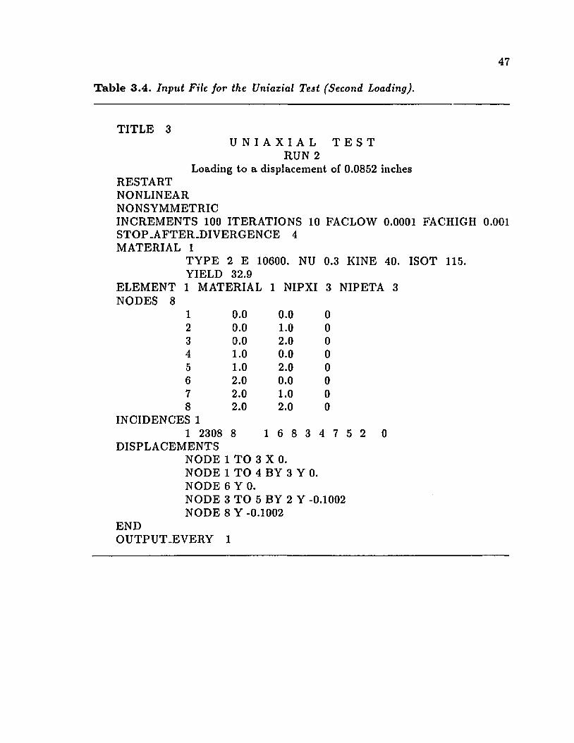
47
Table 3 .4 . Input File for the Uniaxial Test (Second Loading).
TITLE 3U N I A X I A L T E S T
RUN 2Loading to a displacement of 0.0852 inches
RESTARTNONLINEARNONSYMMETRICINCREMENTS 100 ITERATIONS 10 FACLOW 0.0001 FACHIGH 0.001 STOP-AFTER.DIVERGENCE 4
ISOT 115.MATERIAL 1
TYPE 2 E 10600. NU 0.3 KINE 40.YIELD 32.9
ELEMENT 1 MATERIAL 1 NIPXI 3 NIP ETA 3NODES 8
1 0.0 0.0 02 0.0 1.0 03 0.0 2.0 04 1.0 0.0 05 1.0 2.0 06 2.0 0.0 07 2.0 1.0 08 2.0 2.0 0
INCIDENCES 11 2308 8 1 6 8 3 4 7 5 2 0
DISPLACEMENTSNODE 1 TO 3 X 0.NODE 1 TO 4 BY 3 Y 0.NODE 6 Y 0.NODE 3 TO 5 BY 2 Y -0.1002NODE 8 Y -0.1002
ENDOUTPUT.EVERY 1

Table 3.5 . Input File for the Uniaxial Teat (Third Loading).
48
TITLE 3U N I A X I A L T E S T
RUN 3Loading to a displacement of 0.0986 inches
RESTARTNONLINEARNONSYMMETRICINCREMENTS 10 ITERATIONS 10 FACLOW 0.0001 FACHIGH 0.001 STOP-AFTERJDIVERGENCE 4 MATERIAL 1
TYPE 2 E 10600. NU 0.3 KINE 40. ISOT 115. YIELD 32.9
ELEMENT 1 MATERIAL 1 NIPXI 3 NIPETA 3 NODES 8
INCIDENCES 11 2308 8 1 6 8 3 4 7 5 2 0
DISPLACEMENTSNODE 1 TO 3 X 0.NODE 1 TO 4 BY 3 Y 0. NODE 6 Y 0.NODE 3 TO 5 BY 2 Y 0.0134 NODE 8 Y 0.0134
12345678
0.0 0.0 00.0 1.0 00.0 2.0 01.0 0.0 01.0 2.0 02.0 0.0 02.0 1.0 02.0 2.0 0
ENDOUTPUT.EVERY 1

4. SIM U LA TIO N OF C O N TA C T B O U N D A R IE S
4.1 Introduction
Contact problems in general may be classified into two groups, (1) contact be
tween two deformable objects, and (2) contact between a deformable and a rigid
object. Both of the above mentioned classes of contact problems have been ex
tensively studied by a number of researchers. Papers by Hallquist, et. al. [1985],
Lee and Kwak [1984], Padovan and Tovichakchaikul [1984], Wanxie and Suming
[1988], Okamoto and Nakazawa [1979], and Voyiadjis and Poe [1986] extensively
cover most aspects of contact between two deformable bodies. In the study by
Ostachowicz [1984], rigid contact elements were used to model the rigid contacting
bodies.
In this work we need to consider contact between a highly deformable m ate
rial and a rigid forming press or extrusion die. Many successful formulations have
been achieved by using simple geometric shapes such as straight lines and circular
arcs to model the contact boundaries. However, these formulations can model a
limited number of shapes and are often difficult to use. In many situations altering
the shape of the forming press or the die requires additional programming by the
design engineer or the analyst. In finite element solution of metal forming prob
lems, it is necessary to accurately simulate the geometry of the contact boundaries
in an effective and simple way. The design engineer should be able to model a
variety of curved shaped boundaries without having to modify the program.
Generation of curves and surfaces has been the subject of extensive research
by solid modelers and those involved in computer graphics. Many approaches for
generation of curves have been proposed, among these are Besier, Overhauser,
Hermite, and /?-spline formulations (a detailed discussion of these formulations
49

50
may be found in the text book by Foley and Van Dam [1984]). The Besier and
^-spline formulations have gained tremendous popularity for their ease of use in
interactive systems. These methods of curve and surface generation have also
been applied to metal forming problems. Shiau and Kobayashi [1988], used the
Besier surfaces for analysis of three-dimensional open-die forging problems.
In this work the curved contact boundaries are modeled using Hermite para
metric curves. A detailed explanation of this formulation is provided in the fol
lowing sections which may also be applied to /^-splines, Besier and Overhauser
parametric, formulations with only slight modifications. Both tension free con
tact, and fixed rolling contact may be simulated.
4.2 H e rm ite F o rm ula tion o f C ubic C urves
The Hermite form for a cubic parametric curve is determined from the end point
coordinates and corresponding end point tangents. Referring to Figure 4.1, P and
P denote the position vectors of the starting and the finishing points of the curve,
respectively. Similarly, T and T denote the tangent vectors at the corresponding
points P and P respectively. We therefore have
P = p xi + Py j (4.1a)
P = Pxi+ P y j (4.16)
and
T = TI i + r vj (4.2a)
t = f x\ + fy j (4.26)
where i and j are unit vectors along the coordinate axes x and y, respectively.
Assuming a parametric expression for x , we have
x{t) = [M){GX} (4.3a)

51
where
[M] = [t3 , t 2 , t , l ] (4.36)
and
{<?*} = < c (4.3c)I d ;
In equations (4.3a-b), t is a param eter such tha t 0 < t < 1. The objective is to find
the coefficient column vector {C?x} of equation (4.3c) in term s of the end point
position vectors and the corresponding tangents which are given by equations
(4.1a-b) and (4.2a-b), respectively.
For i = 0, from equation (4.3a) we obtain PXJ while for t — 1, we obtain Px .
This is expressed as follows:
®(0 ) = PX = [0,0,0,1 ]{GX} (4.4a)
x ( l ) = A = [ l , l , l , l ] { G ,} (4.46)
Similarly, the derivatives may be obtained by differentiating equation (4.3a) with
respect to t. Consequently we have
x ' ( 0 = \M )'{GX} (4.5)
where x '(t) is derivative of ®(<) with respect to t and [M \ = [3<2 ,2 t, 1,0]. There
fore one obtaines the following:
x'(0) = TX = [0 , 0 , 1,0]{(7Z} (4.6a)
and
x '( \ ) = Tx = [3,2,1,0]{(?Z} (4.66)
The four equations (4.4a-b) and (4.6a-b) can now be cast into a single m atrix
equation as follows:0 0 0 1
0 0 1 o I <4-7)3 2 1 0 .

52
F ig u re 4.1 Hermite Parametric Cubic Curve.
( 0 )
( c )
F ig u re 4.2 Some Possible Shapes of the Hermite Curve.

53
Inverting the 4 x 4 m atrix and solving for the right hand side unknown coefficient
vector {(?*}, we obtain
{<?»} =
2 - 2 1 1 \ ( P * )- 3 3 - 2
- 1 1 J P-0 0 1
0 I Tx1 0 0 0 / I Tx J
= [* ]{ £ ,} (4.8)
where [If] is the 4 x 4 Hermite m atrix and \LX] is the corresponding Hermite
geometry vector which is specified by the user. Substituting equation (4.8) into
equation (4.3a), we obtain
*(<) = [*f]{G .} = [ M ][tf]{£ .} (4-9)
where [G*] is equal to [H ^L *} . A similar param etric expression for y(t) may be
obtained such tha t
y{t) = \M][H]{Ly} (4.10)
where
(4.11)
It m ust be noted tha t in using the Hermite formulation, the term [G*] =
[H]{LX} or [Gj,] = [lf]{ i/y} may be evaluated only once in the solution process.
Any other point on the curve may be evaluated by simply assigning the appropriate
value of the param eter t in the expressions (4.9) and (4.10). In using the Hermite
param etric formulation, the user can control the shape of the curve by specifying
the appropriate end point coordinates and the corresponding tangents at those
points. Some of the possible curved shapes which may be obtained through this
formulation are shown in Figure 4.2.

54
4.3 M o tio n o f th e N o d a l P o in ts on th e C u rv ed B o u n d arie s
Unlike the constraint of motion of a nodal point along a straight boundary, simu
lation of motion along a curved boundary requires updating of the tangent vector
to the curve at the nodal point and continuous correction for possible drift of the
node away from the boundary. Figure 4.3, shows an incremental motion of the
nodal point originally located on the curved boundary at A. Node A is constrained
to move tangentially to the curve at A in the direction of vector during the
current load increment. However, this motion moves node A away from the curved
boundary to a new location denoted by B. For the subsequent load increment, this
node is projected back onto the boundary curve at point C and is constrained to
move tangent to the curve in the direction of vector
In order to locate point C for the drift correction, we need to find the ap
propriate parameter t corresponding to point C. Referring to Figure 4.3, since
vector R, (along BC) is perpendicular to the curve, its scalar dot product with
T*2) should equal to zero. We therefore obtain the following:
( x ° - x b )T±2) + (yc - y B )T™ = 0 (4.12)
where (xB ,y B ) which represent the coordinates of point B are known values ob
tained from the equilibrium state during the last load increment. On the other
hand, (x c ,y c ) and (T ^ , T y 2 ) are unknown and may be expressed in terms of
the unknown parameter t using equations (4.9), (4.10) and (4.5) as follows:
a: 0 = [M]{GX} (4.13a)
y ° = [M]{Gy} (4.13 b)
and
T<!) = {M \{G z} (4.14a)
I f > = [M ]'{G„} (4.146)

55
(2 )
Figure 4.3 Correction Process for the Motion of the Points Gonstrianed to Move on the Die.

56
Substituting equations (4.13a-b) and (4.14a-b) into equation (4.12) will result in
a fifth order polynomial equation in t as shown below:
+ C4 + C2 f2 + c\t + Co — 0 (4.15)
The constants c i , C2 , . . . , c$, in equation (4.15) are given as follows:
c0 = - G x(3)Gx(4) - G y(3)Gy(4) + .xBGx(3) + y BGy{3) (4.16a)
ci = ~(G x(3 ) ) 2 - 2Gx(2)Gx(4) - (Gy(3 ) ) 2
- 2Gy(2)Gy(4) + 2{xb Gx{2) + y B Gy{2 )) (4.166)
c2 = -3G x(l)G x(4) - 3Gx(2)Gx(3) - 3G „(l)G y(4)
- 3Gy(2)Gy(3) + 3(*BG x(l) + y B Gy( 1 )) (4.16c)
c3 = - 2 (Gx(2 ) ) 2 - 4Gx(l)Gx(3) - 2(GV(2 ) ) 2 - 4Gv(l)G y(3) (4.16d)
c4 = -5G x(1)Gz(2) - 5Gy(l)Gy(2) (4.16e)
c5 = -3 (G x ( l ) ) 2 - 3(GV(1 ) ) 2 (4.16/)
where Gx(n) implies the n-tli row of the {G*} column vector. In equations (4.16),
constants C3 ,c 4 and cs are independent of the location of point B and their values
will be calculated only once during the course of the analysis provided that the
curved boundaries do not move. Similarly, the portions of the constants co,ci and
C2 which are independent of the x B and yB will be computed only once, hence
resulting in good computational efficiency.
Once the constants Co through C5 are evaluated, equation (4.15) is solved
numerically for the param eter t. For the solution of the fifth order polynomial
equation in t, the Muller’s m ethod is chosen (Gerald and Wheatley [1985]). This
method converges to the appropriate root of the polynomial within the interval
0 < t < 1 effectively when the first root is obtained. However, there are situations
when the first root obtained may be outside the appropriate range of t, ( 0 < / < 1 ).

57
When this situation arises, synthetic division is used to eliminate the first root
and the program proceeds to find the next root. This process is continued until
the appropriate root t within the required interval is obtained. In this work, it
is assumed that the curved boundaries are reasonable enough and that point B
is sufficiently close to the boundary so that only one normal from point B to
the curve can be drawn. In other words, there is only one root of the equation
(4.15) which is within the interval 0 < t < 1. Once the appropriate value of
the parameter t is determined, the location of point C and the tangent vector
T 12) are respectively evaluated through equations (4.13) and (4.14). Vector R in
Figure 4.3 represents the correction required to bring back the nodal point to the
curved boundary. For the subsequent load increment, the magnitude of vector R
is applied to the restrained direction (direction normal to the boundary at C) as
an imposed displacement and the nodal point is allowed to move along the tangent
direction freely. This process is repeated at the end of every load increment
for all the nodes that are in contact with the curved boundaries.
4.4 U se o f M ultip le C urves in G en era tin g C om plex B oundaries
Quite frequently the curved boundaries involved in contact problems have complex
shapes which may not be represented by a single cubic parametric curve. Also,
there are situations where multiple boundaries need to be identified. In these
situations it is necessary to use multiple splines to represent the appropriate shape
of the boundaries. This task is achieved easily in UNIFES by simply allowing the
user to define multiple geometry vectors in order to generate multiple Hermite
curves.
One major problem in using multiple curve definitions for representing the
boundaries is the task of identifying the closest curve to a given interface node.

58
The procedure described in the earlier section for controlling the motion of the
nodal points on the boundaries is applicable, but additional information is needed
to eliminate the unnecessary and time consuming solution of the fifth order poly
nomial of equation (4.15) for the curve segments which are not close to a given
nodal point. Also, there are situations where there is a possibility to draw a
normal line from one nodal point to more than one curve segment. Figure 4.4,
illustrates this situation. In Figure 4.4, node A should be constrained to move on
curve C. However, the procedure described in the previous section can mistakenly
identify curve C' as the constraining boundary for node A.
The above mentioned problems are eliminated by identifying an inclusion
zone for each curve segment. If the coordinates of the node under consideration
are within the bounds of the inclusion zone of a curve segment, then the node
is constrained by the curve and the procedure of section 4.3 is applied to that
particular curve segment.
The inclusion zone for each curve segment is identified by the user through
specifying the lower-left and the uper-right hand corners of a box containing the
spline. It is possible for the inclusion zone of two splines to overlap. If this situation
arises, both curve segments are checked and the first curve with its normal passing
through the nodal point is chosen as the constraining curve.

59
r
F ig u re 4.4 . Zoning of the Contact Boundaries.

4.5 D escrip tion o f th e R elevant S u b ro u tin es
60
A complete listing of the module necessary for controlling the motion of the nodal
points on the curved boundaries is provided in Appendix D. The control program
for this module is subroutine BOUND. This module is called by the finite element
control program prior to start of each new load increment in order to update the
boundary conditions and the orientation of the skew rollers. A brief description
of each subroutine belonging to this module is provided next.
S u b ro u tin e B O U N D . This subroutine is the main control module for determin
ing the location of the interface node (nodes that may become in contact with the
boundary during the course of the analysis). The appropriate direction cosine vec
tors (COSTX, COSTY), the incremental load vector (RINC), and the incremental
displacement vector (UINC) are updated appropriately based on the motion and
the location of the interface nodes. The parameter ICODE is set equal to zero
if recalculation of the degree of freedom vector ID OF is not necessary, otherwise
ICODE is set equal to unity.
S u b ro u tin e H E R M IT E . This subroutine is addressed only once during the
course of the analysis in order to calculate the {Gx} and {Gy} column vectors as
given by equation (4.8). This program is called by the main finite element module
at the start of the program.
S u b ro u tin e C O E F . This subroutine is addressed only once in order to calculate
the coefficients 0 3 , 0 4 and 0 5 and the constant part of the coefficients co,cj and
Co using equations (4.16a-f). This subroutine is called by the main finite element
module at the start of the program.
S u b ro u tin e H E R M X Y . This sibroutine is used to evaluate the x and y coor

61
dinates of a point on the curved boundary using equations (4.9) and (4.10).
S u b ro u tin e X Y P R IM . This subroutine calculates the tangent vector to the
curve given by equation (4.5).
S u b ro u tin e M U L L E R . This subroutine evaluates the additional parts of con
stants Co,Ci and C2 which depend on the location of the node at point B (refer
to Figure 4.3). It subsequently checks the position of the nodal point against the
inclusion zone for each curve in order to eliminate the curves which are not close
to the point. Afterwards, the Muller’s method with synthetic division is used to
find the appropriate parameter t for the fifth order polynomial given by equation
(4.15). If a root is not found within the interval 0 < t < 1, the flag IRET is set
equal to zero. This indicates to program BOUND that the node is free.

5. P A R A M E T R IC S T U D Y O F A X IS Y M M E T R IC E X T R U S IO N
5.1 In tro d u c t io n
The problem of axisymmetric m etal extrusion is investigated in this work. The
billet is ten inches long with a radius of one inch and is made of the aluminum
alloy 2024 T4. The m aterial param eters used in the constitutive model (refer to
C hapter 3) for this aluminum alloy are presented in Table 5.1. In Table 5.1, crv is
the initial yield for uniaxial loading. The determ ination of param eters b and c is
discussed by Voyiadjis [1984] and Voyiadjis and Kiousis [1987].
T ab le 5.1. Material Properties for Aluminum 202^-Tf.
Modulus of E lasticity .................................................................................. E = 10,600fcstPoisson’s R a tio ........................................................................................................... v = 0.3Kinematic Hardening P aram eter....................................................................... b = 40ksiIsotropic Hardening P aram ete r......................................................................c = 115A:stInitial Yield Stress (From Uniaxial Loading)............................................. av = 57ksi
The contact surface between the billet and the rigid die is assumed to be
friction free. This in general is a valid assumption because lubricants are often
used in extrusion processes. Referring to Figure 5.1, the die is modeled using
three Hermite curves, namely AB, BC and CD. Portion AB represents a cylinder of
constant radius th a t encloses the undeformed billet as shown in Figure 5.1. Region
BC is the reduction region of the die and is obtained through a Hermite curve with
horizontal tangents at both ends B and C. These horizontal tangents provide for a
smooth transition of the material from one segment of the die to another. The exit
portion of the die CD provides a region for the smooth recovering of the elastic
strains and for unloading of the m aterial. In the finite element formulation the
62

63
billet is modeled such that it slides on the rigid die with tension free contact. This
formulation allows the material to separate from the die as soon as tensile forces
develop between the die and the billet. In the case when a previously released
node penetrates the die, that node is again constrained to roll smoothly on the
die surface.
Initially the billet is placed in region AB with a slight penetration of 0.05
inches into segment BC. This is to ensure that an axial force developes for the
very first load increment. The billet is pushed through the die using a displacement
control approach. A total displacement of 5 inches is applied to the left end of the
billet using 250 load increments (0.02 inch per load increment) during the process
of extrusion.
The convergence criterion used in this finite element analysis is based on the
incremental internal energy obtained at the end of each iteration. The incremen
tal internal energy defined during the ith iteration of the n th load increment is
expressed as follows:
A £/<<> = (5.1)
where iZen^ end are equilibrium load vectors at the n th load increment
for the ith and (i — l) th iterations respectively. These equilibrium load vectors
are obtained from the element stresses. In equation (5.1), A r e p r e s e n t s the
displacement increments at the ith iteration of the nth load increment. It is
assumed that the convergence is obtained provided:
A U™ < eA U™ ( 5 .2 )
where e is a tolerance factor and A Un^ is the internal energy obtained at the first,
iteration of the n th load increment. Similarly divergence is implied when
A UP > A UW (5.3)

Figure 5.1. Schematic Representation of the Die and the Initial Position of the Billet.
Oi>u

65
During the course of the analysis, it is observed that for some load increments
the proposed iterative solution procedure either diverges or does not converge to
the prescribed limit within the prescribed maximum allowable number of iter
ations. When this occurs, the load step is reduced to one-half of the previous
load increment and the procedure is repeated until ail the load for this particu
lar load increment is applied. This automatic procedure for the reduction of the
load increment is only applied to those particular load increments with conver
gence problems; hence, it does not affect the loading procedure for any subsequent
increments.
T able 5.2. Parameters Used for the Control of the Iterative Solution Process.
Strictest convergence tolerance.............................................cmax = 10“ 7
Least acceptable convergence tolerance.............................. cmtTl = 10- 4
Allowable number of diverging ite ra tions............... .......................................... Nd = 4Maximum allowable number of iterations per load increm ent.................... N = 10
The parameters listed in Table 5.2, are utilized for the control of the iterative
solution procedure used in this work. During each load increment, the tolerance
f-max is used in relation (5.2) in order to test for convergence. In case the criterion
expressed by relation (5.2) using emax is not m et, the corresponding value of e
required to satisfy the equality of relation (5.2) is computed. Should the computed
value of e fall within the bounds of emaI and emin, then the solution is assumed
to have converged and the next load increment is applied. Nevertheless, this
relaxed convergence criterion is only accepted for a specified limited number of load
increments. The param eter Nd indicates how many times relation (5.3) should
be satisfied (divergence occurs) for a given load increment prior to applying the
automatic subincrementation for the diverging load increment.

66
5.2 C om parison o f D ifferent E lem ent T ypes and M eshes
A series of preliminary analyses are made using five different meshes each with
different types of elements. The characteristics of the meshes used for each one
of these runs are indicated in Table 5.3. The same die model is used for all five
runs which are presented in this section. The initial one inch radius of the billet is
reduced to 0.8 inches after extrusion. This is equivalent to a 36% reduction in the
cross-sectional area of the billet. The die angle used is approximately 7.59 degrees.
Referring to Figue 5.1, the die angle is approximated by connecting points B and
C by a straight line and measuring the angle <f> which this line makes with a
horizontal line. The parameters used to generate each segment of the die for these
runs are listed in Table 5.4. These runs are made for the purpose of determining
the optimum mesh in terms of accuracy of the results, efficiency of analysis and
handling of singularities which in particular arise at the exit of the die. Figure
5.2, illustrates the meshes used for each run.
Table 5.3. Mesh Characteristics for Runs A l Through A5^.
Run
Numberof
Nodes in Element*
Numberof
Elements
Number of Integration Points per
Element
Aspect Ratio of
Elements Nodes
Total Number of
Integration Interface Points Nodes
A l 4 320 4 2 369 1,280 40A2 4 640 4 1 729 2,560 80A3 8 320 9 2 1,057 2,880 80A4 9 320 9 2 1,377 2,880 80A5 4,5,8 640 4,9 1 970 2,960 160
f All runs are based on a 36% reduction in the area and a die angle of 7.59 degrees. * All elements are isoparametric quadrilateral elements.

It is observed that run Al using a mesh composed of 320 four-noded elements
fails to complete the extrusion problem. Divergence occurs at load increment
84, that is when the second column of elements exit the die. Automatic load
subincrementation procedure described earlier fails to correct the divergence. Run
A2 using 640 four-noded elements, also fails to complete the analysis. However,
this time divergence occurs at load increment 1 2 2 , that is when the left end of the
billet is displaced by 2.44 inches (6.2 cm). Further mesh refinement using the four-
noded isoparametric element will be computationally inefficient when compared
to meshes used utilizing eight or nine noded elements in runs A3, A4 and A5.
T able 5.4. Parameters Used to Generate the Die for Runs A l Through A5 Using the Hermite Formulation.
segment K V r ; r p * *K P**
Vr p *
Xr p * *
V
AB 1.0 0.0 0.0 2.0 1.0 9.95 0.0 2.0BC 1.0 9.95 0.0 2.0 0.8 11.45 0.0 2.0CD 0.8 11.45 0.0 0.7 0.85 11.95 0.08 0.4
* x-direction corresponds to the radial direction. ** y-direction corresponds to the axis of symmetry of the billet.
Runs A3 and A4 are successfully completed with the m aterial extruded as
specified previously. However, use of 320 nine noded Lagrangian isoparametric
elements in run A4 does not lead to improved performance or better results over
the same number of eight-noded elements used for run A3. The extrusion pressure
is obtained at the end of each load increment. The pressure versus the displace
ment of the left end of the billet is presented for runs A2, A3 and A4 in Figures
5.3 through 5.5. It is seen that the extrusion pressure increases steadily up to
approximately a displacement of 1.6 inches. This range of steady increase of the
extrusion pressure corresponds to the case when the billet fills the die. As the

68
MESH USED FOR RUN A I
MESH USED FOR RUN A2
MESH USED FOR RUN A3
MESH USED FOR RUN A4
MESH USED FOR RUN A5
F ig u re 5 .2 . Meshes Used for Runs A l Through A5.
71

69
billet exits the die, the interface nodes tha t are constrained to move on the die
are released. This causes a drop in the elastic strain energy of the billet which
in turn causes a drop in the extrusion pressure. As the material continues to
enter the die, the next interface node due to be released continues to move on
the die until it reaches the exit point of the die. During this period, the strain
energy of the billet continues to increase hence increasing the extrusion pressure.
This process will continue as shown in Figures 5.3 through 5.5 until the billet has
completely exited the die. It must be noted tha t this condition does not exist
in real extrusion problems. This is because as one material point on the surface
of the billet exits the die, there is another m aterial point infinitesimally close to
the previous point which is still constrained to move on the die. In finite element
analysis, the nodes that are released as the billet exits the die are a finite distance
apart, consequently resulting in the above mentioned fluctuations in the extrusion
pressure. Ideally, as one decreases the distance between the constrained nodes,
these fluctuations are phased out. The studies performed by Aravas [1986] and
Nagtegaal and Veldpaus [1980], confirm the existence of these fluctuations in the
numerical solution of metal extrusion problems.
Run A5 is used to verify tha t these fluctuations are a function of the distance
between the interface nodes. The mesh used in this run consists of 640 elements
(eight elements in the radial direction and eighty elements along the length of the
billet). The row containing 80 elements at the interface with the die is made of
eight-noded quadratic isoparametric elements. The second row next to the inter
face is made of five-noded quadrilateral isoparametric transition elements. These
elements are used to provide transition from a quadratic displacement field to a
bi-linear displacement field. All subsequent rows are m ade of four-noded quadri
lateral elements (refer to Figure 5.2). This mesh is computationally as efficient
as the mesh for run A3 which uses 320 eight-noded quadrilateral isoparametric

Extr
usio
n Pr
essu
re
(KSI
)
1 0 0 . 0 0 - r
90.00 - -
80.00 - -
70.00 - -
60.00
50.00 - -
30.00
20.00 - -
10.00 - -
0.000.25 0.500.00 0.75 1.00 1.25 1.50 1.75 2.252.00 2.50
Displacement (in.)
Figure 5.3. Extrusion Pressure Versus Displacement for Run AS (Incomplete Extrusion).

Ext
rusi
on
Pres
sure
(K
SI)
90.00 -r
70.00 - -
60.00 --
50.00 - -
40.00 - -
30.00 - -
20.00
10.00 - -
0.000.50 1.500.00 1.00 2.00 3.00 3.50 5.00 5.504.00 4.50
Displacement (in.)
Figure 5.4. Extrusion Pressure Versus Displacement for Run A3.

Extr
usio
n Pr
essu
re
(KSI
)
90.00
80.00 - -
70.00 - -
60.00
50.00 - - U--- 1
40-00
30.00 - -
20.00 ■I-
10.00
0.000.00 0.50 1.50 3.00 3.502.00 2.50 4.50 5.004.00 5.50
Displacement (in.)
Figure 5.5. Extrusion Pressure Versus Displacement for Run A j.

73
elements. However, the distance between the interface nodes for run A5 is one-half
of tha t used for run A3. Figure 5.6 shows the extrusion pressure versus the dis
placement for the left end of the billet for run A5. Comparison of this figure with
Figures 5.3 through 5.5 indicates that the amplitude of the fluctuations decreases
substantially when the mesh for run A5 is used.
It is also noted tha t the fluctuations shown in Figures 5.4 through 5.6 consist
of a high peak followed immediately by a low peak. As shown in Figure 5.6,
This corresponds to the release of the middle node followed by the release of the
neighboring corner node of the quadratic elements respectively. Figure 5.3 which
corresponds to run A2 does not show this characteristic because the elements
used there at the interface with the die are four-noded isoparametric elements.
Therefore, all the fluctuation peaks in Figure 5.3 are identical. We m ust also note
tha t the distance between the respective peaks is identical to the distance between
the neighboring nodes at the interface of the die.
The above mentioned fluctuations may be further reduced by incrementally
removing the load on the released nodes as presented by Aravas [1986]. It must
be noted however, that this m ethod does not completely remove the fluctuations
and will lead to an extrusion pressure which is significantly higher than the actual
extrussion pressure. The higher extrusion pressure is caused by the fact that
sustaining an artificial load on the exiting nodes will provide additional resistance
to the flow of the m aterial through the die.
Figures 5.3 through 5.6 also show tha t the extrusion pressure increases steadily
until the material fills the die. Thereafter, the pressure decreases until a steady
state condition is reached. This finding is identical for runs A l through AS re
gardless of element types.

Ext
rusi
on
Pre
ssur
e (K
SI)
90.00
80.00
70.00
60.00
50.00
40.00
30.00
20.00
10.00
0.000.00 0.50 1.00 1.50 2.00 2.50 3.00 3.50 4.00 4.50 5.00 5.50
Displacement (in.)
Figure 5.0. Extrusion Pressure Versus Displacement for Run A5.
HIGH PEAK
LOWPEAK
i i i | m n | i i i t | i i l i | i i i i | i i i i | i 'i m | i m i | i i i i | i m i | m r i

75
5.3 Num erical R esults Obtained U sing Run A5
In Figure 5.7, the distribution of the yield zone at various stages of the extrusion is
shown. It is observed that subsequent to exiting the die, yielding continues at some
integration points. This is primarily due to the fact that the extruded material is
seeking a final equilibrium state which may only be reached by additional yielding
of the material until the residual stresses balance themselves.
In Figures 5.8 through 5.11, the stress intensity contours are plotted for both
the Cauchy stress and the second Piola-KirclihofF stress components. Two regions
of heavy stress concentrations are observed in the stress contours. We note that
at the entrance of the reduction region of the die (location B in Figure 5.1) and at
the exit of the die, large stress variations are observed. This in particular is more
intense for the axial and shear stress distributions. Variation of the axial stress
distribution indicates that after extrusion, compressive axial stresses occur near
the core of the billet and tension forms towards the outer radius of the billet. It is
also seen that stresses at the free end of the extruded material vary significantly
without showing distinct patterns.
In Figure 5.8, section A-A indicates an appropriate section for obtaining the
residual stresses for the extruded material. The regions closer to the free end of
the billet or the exit of the die are affected by the stress concentrations and should
not be used to record the residual stresses for the final product.
Figure 5.12, shows the distribution of the volumetric Cauchy stress compo
nents. The highest compressive volumetric stresses occur in the immediate vicin
ity of segment BC of the die (reduction region). The maximum tensile volumetric
stresses occur at the free end of the extruded billet and also at the axis of the
billet after extrusion.
In Figures 5.13 and 5.14 the Lagrangian strain variations are shown. The
highest shear strain value observed in Figure 5.14 is -31.96 percent which occurs

Figure 5.7. The Yield Zone at Various Stages of the Extrusion for Run A5.
-i05

DISTRIBUTION OF THE 2ND P.K. RADIAL STRESS AT LOAD STEP 250 (KSI) MINIMUM = - 0 .3660E+03 MAXIMUM = 0.9490E+020 = -0.3587E+03 1 = -0.3085E+03 2 = -0.2583E+03 3 = -0.2081E+034 = - 0 . I579E+03 5 = -0.1077E+03 6 = -0.5755E+02 7 = -0.7368E+018 = 0.4282E+02 9 = 0.9300E+02
DISTRIBUTION OF THE RADIAL CAUCHY STRESS AT LOAD STEP 250 (KSI)MINIMUM = -0.2167E+03 MAXIMUM = 0.5532E+020 = -0.2124E+03 1 = -0.1828E+03 2 = -0.1532E+03 3 = -0.1235E+034 = -0.9391E+02 5 = -0.6429E+02 6 = -0.3466E+02 7 = -0.5039E+018 = 0 .2459E+02 9 = 0.5421E+02
* ~ j-'iFigure 6.8. Radial Stress Distribution for Run A5.

1 0 0 1 1 1 1 1 3 2 2 3 1 5 6 7 8 8 7 6 5 1 1 5
DISTRIBUTION OF THE 2ND P.K. AXIAL STRESS AT LOAD STEP 250 (KSI) MINIMUM = -0.9018E+02 MAXIMUM = 0.8603E+020 = 0.8838E+02 1 = 0.6919E+02 2 = 0.5000E+02 3 = 0.3081E+024 = 0.1163E+02 5 = -0.7561E+01 6 = -0.2675E+02 7 = -0.4594E+028 = -0.6512E+02 9 = -0.8431E+02
2 2 3 5 5 1 3 2 1 1 2 3 1 5 6 7 8 8 7 6 5 1 1
DISTRIBUTION OF THE CAUCHY AXIAL STRESS AT LOAD STEP 250 (KSI)MINIMUM = - 0 .1615E+03 MAXIMUM = 0.1614E+030 = 0 .1583E+03 1 = 0 .1231E+03 2 = 0.8796E+02 3 = 0.5280E+024 = 0.1764E+02 5 = -0.1753E+02 6 = -0.5269E+02 7 = -0.8785E+028 = - 0 .1230E+03 9 = -0.1582E+03
ooFigure 5.9. Axial Stress Distribution for Run A5.
l/l
CP

1 3 2 2 3 4 5
DISTRIBUTION OF THE 2ND P.K. SHEAR STRESS (RZ) AT LOAD STEP 250 (KSI) MINIMUM = -0.5202E+02 MAXIMUM = 0.5801E+020 = - 0 .5098E+02 1 = -0.3900E+02 2 = -0.2702E+02 3 = -0.1504E+024 = - 0 .3056E+01 5 = 0.8925E+01 6 = 0.2091E+02 7 = 0.3289E+028 = 0.4487E+02 9 = 0.5685E+02
4 2 2 33 4 5 5 5
DISTRIBUTION OF THE SHEAR CAUCHY STRESS (RZ) AT LOAD STEP 250 (KSI)MINIMUM = -0.5184E+02 MAXIMUM = 0.5804E+020 = -0.5081E+02 1 = -0.3884E+02 2 = -0.2688E+02 3 = -0.149IE+024 = -0.2945E+0I 5 = 0.9020E+01 6 = 0.2098E+02 7 = 0.3295E+028 = 0.4492E+02 9 = 0.5688E+02
- ~ icoFigure 5.10. Shear Stress Distribution for Run A5.

6 5 6 5 H 3 2 6 6 6 6 5 5 G
DISTRIBUTION OF THE 2ND P.K. CIRCUMFERENTIAL STRESS AT LOAD STEP 250 (KSI) MINIMUM = -0.3795E+03 HAXIMUM = 0.145BE+030 = -0.3719E+03 I = -0.3147E+03 2 = -0.2575E+03 3 = -0.2003E+034 = -0.1431E+03 5 = -0.8589E+02 6 = -0.2869E+02 7 » 0.2850E+028 = 0.8570E+02 9 = 0.1429E+03
5 56 6 6 6 6 5 G
DISTRIBUTION OF THE CIRCUMFERENTIAL CAUCHY STRESS AT LOAD STEP 250 (KSI)MINIMUM = -0.3208E+03 MAXIMUM = 0.1192E+030 = -0.3144E+03 1 = -0.2665E+03 2 = -0.2186E+03 3 = -0.1706E+034 = - 0 .1227E+03 5 = -0.7481E+02 6 = -0.2690E+02 7 = 0.2102E+02
8 = 0.6894E+02 9 = 0.1169E+03ooo
Figure 5.11. Circumferential Stress Distribution for Run A5.

9 5 5 1 3 75 6 7 7 7 6 6
DISTRIBUTION OF THE VOLUMETRIC STRESSES AT LOAD STEP 250 (KSI) MINIMUM = -0.2121E+03 MAXIMUM = 0.8023E+020 = -0.2078E+03 1 = -0.1760E+03 2 = -0.1442E+03 3 = “0.1123E+034 = -0.8051E+02 5 = -0.4869E+02 6 = -0.1686E+02 7 = 0.1497E+028 = 0.4679E+02 9 = 0.7862E+02
Figure 5.12. Cauchy Volumetric Stress Distribution for Run A5.
oo

g 8 6 4 2 1 I 2 3
DISTRIBUTION OF THE RADIAL STRAIN AT LOAD STEP 250 HINIMUM = - 0 .1971E+00 MAXIMUM = 0.8883E-030 = - 0 .1931E+00 1 = - 0 .1716E+00 2 = -0.1500E+00 3 = -0.1285E+00A = -0.1069E+00 5 = -0.8535E-01 6 = -0.6380E-01 7 = -0.A22AE-018 = -0.2069E-01 9 = 0.8707E-03
1 3 5 7 8 80 7 6
DISTRIBUTION OF THE AXIAL STRAIN AT LOAD STEP 250 MINIMUM = -0.7304E-02 MAXIMUM = 0.7516E+00
0 = -0.7157E-02 1 = 0.7548E-01 2 = 0.1581E+00 3 = 0.2A08E+00A = 0.323AE+00 5 = 0.A060E+00 6 = 0.A887E+00 7 = 0.5713E+008 = 0.65A0E+00 9 = 0.7366E+00
ootoFigure 5.13. Radial and Axial Strain Distributions for Run A5.

5 5
DISTRIBUTION OF THE SHEAR STRAIN (RZ) AT LOAD STEP 250 MINIMUM = -0.3196E+00 MAXIMUM = 0.1758E+000 = - 0 .3132E+00 1 = -0.2592E+00 2 = -0.2053E+00 3 = -0.1514E+004 = -0.9742E-01 5 = -0.4348E-01 6 = 0.1047E-01 7 = 0.6441E-018 = 0 .1184E+00 9 = 0 .1723E+00
7 5 3 ! 0 09 1 1 1 2
DISTRIBUTION OF THE CIRCUMFERENTIAL STRAIN AT LOAD STEP 250 MINIMUM = - 0 .1883E+00 MAXIMUM = 0.8875E-030 = - 0 .1845E+00 1 = - 0 .1639E+00 2 = -0.1433E+00 3 = -0.1227E+004 = -0.1021E+00 5 = -0.8152E-01 6 = -0.6092E-01 7 = -0.4033E-018 = -0.1973E-01 9 = 0.8699E-03
Figure 5.14. Shear and Circumferential strain Distributions for Run A5.00W

1 3 5 7 7 7 7
DISTRIBUTION OF THE PLASTIC-WORK INTENSITY AT LOAD STEP 250 (KSI)MINIMUM = 0.0
0 = 0.7157E-01 1 =4 = 0 .2649E+02 5 =8 = 0.5305E+02 9 =
MAXIHUH = 0.6569E+01 0.3313F.+02 0.5969E+02
0.6091E+02
2 = 0 .1321E+02 3 = 0.1985E+026 = 0.3977E+02 7 = 0.4641E+02
Figure 5.15. Distribution of the Plastic Work Intensity for Run A5.
00

85
at the center of the reduction region. It is observed in Figure 5.13 that the axial
strain for the extruded billet has almost a constant value of 65.4 percent. However,
the maximum axial strain is 75.16 percent at the free end of the extruded billet.
The distribution of the plastic work intensity k is depicted in Figure 5.15. As
anticipated, the maximum plastic work occurs at the outer radius of the extruded
billet which undergoes higher shear strains than regions closer to the core of the
billet. The value of k as used in the expression for the yield surface determines
the extend of the isotropic liardeneing of the material.
5.4 Study o f Various Area R eduction and Die Angle Changes
In order to study the effect of changes in the percent reduction of the cross-
sectional area and also the die angle on the extrusion pressure a series of nine
analyses are performed. The characteristics of each analysis is shown in Table 5.5.
As is seen in this table, these runs are made for 25, 30, and 35 percent reductions
in the area and also for die angles of 5, 7, and 9 degrees. These numbers are
selected because they represent logical values which are used in most extrusion
applications. Die angles which are greater than ten degrees have been known to
cause large tensile volumetric stresses in the billet which lead to the development of
voids in the material. The same reasoning also applies to large reduction ratios in
the cross-sectional area of the billet. Tables 5.6 through 5.14 show the parameters
used to generate the die for each case.
Figures 5.16 through 5.18 show the extrusion pressure versus the displace
ment of the left end of the billet for analysis groups B, C and D respectively. As
is seen in these figures the extrusion pressure increases as the die angle increases.
This is logical because a larger angle tends to reduce the cross-sectional area of the
billet over a shorter distance, therefore requiring a larger driving force. Figures

86
T able 5.5. Identification Codes fo r Each Analysis
% Area Reduction
Die Angle 25 30 35
9 Degrees B1 C l D 1
7 Degrees B2 C2 D25 Degrees B3 C3 D3
5.16 through 5.18 also indicate that as the die angle increases the amplitude of the
fluctuations in the extrusion pressure increases as well. This confirms the obser
vations made in the preceeding section that the amplitude of these fluctuations is
directly related to the elastic strain energy of the material. The larger extrusion
pressure for sharper die angles induces higher levels of elastic strain energy in the
billet; hence, the amplitude of the fluctuations is increased.
Figure 5.19 illustrates the change in the steady-state extrusion pressure for
various reduction ratios as the die angle increases. It is observed that the variation
in the steady-state pressure with respect to the die angle is linear. However,
the slope of the curves in Figure 5.19 increases slightly as the reduction ratio is
increased. Figure 5.20 shows the relation between the peak extrusion pressure and
the die angle. In this case the curves are not perfect straight lines.
Figures 5.21 and 5.22 illustrate the steady-state and the peak extrusion pres
sures versus the percent reduction in area for various die angles, respectively. It
is again observed that the curves in these figures represent relations which are
approximately linear. It is also observed tha t as the die angle increases the slope
of the curves increases slightly.

87
T able 5 .6 . Parameters used to generate the die for run B l .
segment p ; p * *y t : r p * *
V P*■* X r vr p * r p * *
AB 1 . 0 0 . 0 0 . 0 2 . 0 1 . 0 9.95 0 . 0 2 . 0
BC 1 . 0 9.95 0 . 0 0.5 0 . 8 6 6 10.796 0 . 0 0.5CD 0 . 8 6 6 10.796 0 . 0 0.7 0.916 11.296 0.08 0.4
T ab le 5.7. Parameters used to generate the die for run B2.
segment p ; P**r y T*-*■ Xr p * * P* •* * P** J v
r p * X X
r p * *x y
AB 1 . 0 0 . 0 0 . 0 2 . 0 1 . 0 9.95 0 . 0 2 . 0
BC 1 . 0 9.95 0 . 0 0.7 0 . 8 6 6 11.041 0 . 0 0.7CD 0 . 8 6 6 11.041 0 . 0 0.7 0.916 11.541 0.08 0.4
T able 5.8. Parameters used to generate the die for run B3.
segment p ; P**y t ; r p * *V p ; p . *
V T *X r p * *V
AB 1 . 0 0 . 0 0 . 0 2 . 0 1 . 0 9.95 0 . 0 2 . 0
BC 1 . 0 9.95 0 . 0 1 . 0 0 . 8 6 6 11.482 0 . 0 1 . 0
CD 0 . 8 6 6 11.482 0 . 0 0.7 0.916 11.982 0.08 0.4
T able 5.0. Parameters used to generate the die for run Cl.
segment p : p * .V
T* r p * * P*1 XP * *
Vr p *1 X
r p * *V
AB 1 . 0 0 . 0 0 . 0 2 . 0 1 . 0 9.95 0 . 0 2 . 0
BC 1 . 0 9.95 0 . 0 0.7 0.8367 10.981 0 . 0 0.7CD 0.8367 10.981 0 . 0 0.7 0.8867 11.481 0.08 0.4
T ab le 5 .10. Parameters used to generate the die for run C2.
segment p* P **y t : r p * *1 y P *1 X P**y
r p *^ X
r p * ** V
AB 1 . 0 0 . 0 0 . 0 2 . 0 1 . 0 9.95 0 . 0 2 . 0
BC 1 . 0 9.95 0 . 0 1 . 0 0.8367 11.28 0 . 0 1 . 0
CD 0.8367 11.28 0 . 0 0.7 0.8867 11.78 0.08 0.4

88
Table 5.11. Parameters used to generate the die for run CS.
segment P *•* * P **r yr p * r p * *
p : P**■‘ v t ; r p * *x y
AB 1 . 0 0 . 0 0 . 0 2 . 0 1 . 0 9.95 0 . 0 2 . 0
BC 1 . 0 9.95 0 . 0 1.5 0.8367 11.817 0 . 0 1.5CD 0.8367 11.817 0 . 0 0.7 0.8867 12.317 0.08 0.4
Table 5.12. Parameters used to generate the die for run D l.
segment p ; ^ V T***• Xrp**
p : n** r p *J. j .r p + *x y
AB 1 . 0 0 . 0 0 . 0 2 . 0 1 . 0 9.95 0 . 0 2 . 0
BC 1 . 0 9.95 0 . 0 0 . 8 0.806 11.175 0 . 0 0 . 8
CD 0.806 11.175 0 . 0 0.7 0.856 11.675 0.08 0.4
Table 5.13. Parameters used to generate the die for run D2.
segment p : D**V
r p *X
r p * *p : P ** r p *
^ Xr p * *±y
AB 1 . 0 0 . 0 0 . 0 2 . 0 1 . 0 9.95 0 . 0 2 . 0
BC 1 . 0 9.95 0 . 0 1 . 0 0.806 11.53 0 . 0 1 . 0
CD 0.806 11.53 0 . 0 0.7 0.856 12.03 0.08 0.4
Table 5.14. Parameters used to generate the die for run D3.
segment p : p** T* r p * *V p : P **
Vr p *
Xr p * *
AB 1 . 0 0 . 0 0 . 0 2 . 0 1 . 0 9.95 0 . 0 2 . 0
BC 1 . 0 9.95 0 . 0 1.5 0.806 12.167 0 . 0 1.5CD 0.806 12.167 0 . 0 0.7 0.856 12.667 0.08 0.4

Ext
rusi
on
Pre
ssur
e (K
SI)
50.00
45.00
40.00
35.00
30.00
25.00
20.00
15.00
10.00
5.00
0.000.00 0.50 1.00 1.50 2.00 2.50 3.00 3.50 4.00 4.50 5.00 5.50
Displacem ent (in.)
Figure 5.16. Extrusion Pressure Versus Displacement for Runs B l, B2, and B3.
n T 'i r i i i I i i i i |

Ext
rusi
on
Pre
ssur
e (K
'S!)
‘ 0.00 - r
60.00
50.00 - -
40.00 - -
30.00 - -
20.00 - -
10.00 - -
0.00 -
0.00
I
i i i | i r i i l i i i i | n i l | i i i i j n n | n i t ; i 0.50 1.00 1.50 2.00 2.50 3.00 3.50
Displacem ent (in.)
I | - I I l r | I 4.00 4.50
i i i | i r i i 5.00 5.50
Figure 5.17. Extrusion Pressure Versus Displacement for Runs C l, CS, and CS.

Extr
usio
n Pr
essu
re
(KSI
)
90.00
s o . o o
70.00
60.00
50.00
40.00
30.00
20.00
10.00
0.000.00 0.50 1.00 1.50 2.00 2.50 3.00 3.50 4.00 4.50 5.00 5.50
Displacem ent (in.)
Figure 5.18. Extrusion Pressure Versus Displacement, for Runs D l, DS, and D3.

tead
y-S
tate
E
xtru
sion
P
ress
ure
(KSt
)
60.00 - r
55.00 - -
50.00 - -
40.00
35.00 - -
30.00 - -
in
20.005.00 6.00 6.504.50 5.50 B.OO B.50 9.00
Die Angle (D egrees)
Figure 5.19. Steady-State Extrusion Pressure Versus the Variation in the Die Angle. t o

Peak
E
xtru
sion
P
ress
ure
(KSI
)
85.00 -r
80.00
75.00
70.00
65.00
60.00
55.00
50.00
45.00
40.00
35.00
30.00
25.004.50 6.50 7.00 7.50
Die Angle (D egrees)5.00 5.50 6.00 8.00 8.50 9.00 9.50
Figure 5.20. Peak Extrusion Pressure Versus the Variation in the Die Angle.

Ste
ady-
Sta
te
Ext
rusi
on
Pre
ssur
e (K
Sl)
6 0 .0 0 - r
55.00 - -
50.00 - -
45.00 - -
40,00 - -
^ > T•De# e i !
30.00 - -
25.00 - - -v
20.0024.00 25.00 26.00 27.00 28.00 29.00 30.00 31.00 32.00 33.00 34.00 35.00 36.00
% Reduction in Area
Figure 5.21. Steady-State Extrusion Pressure Versus the % Reduction in Area. CO

Peak
E
xtru
sion
Pr
essu
re
(KSI
)
B5.0O
530.00
75.00
70.00
65.00
60.00
55.00
50.00
35.00
24.00 25.00 26.00 27.00 28.00 29.00 30.00 31.00 32.00 33.00 34.00 35.00 36.00
% Reduction in Area
Figure 5.22. Peak Extrusion Pressure Versus the % Reduction in Area.

6. U N IF E S U SE R S G U ID E
6 .1 . In tro d u ctio n
In this chapter the reader is familiarized with the UNIFES input commands and
the syntax that must be followed in order for these commands to be recognized
properly by the program.
UNIFES uses unformated input files which may include character strings as
well as numeric data. Character strings should not be enclosed in quotes. The
command processor COMPRO selects the first four characters from each character
string and uses them to form a simplified four byte long command which is then
recognized by the program. A blank space may not be used in a character string
which represents a single command. However, a blank space may be used in
between different commands and /o r numeric data. For example the character
string INTERFACE.NODES is recognized as a single command. The command
processor selects the first four characters INTE to have a special meaning. The
character strings INTE or INTEABCDEFG are interpreted by the program to
have the same meaning as the character string INTERFACE.NODES. Notice that
the underline between the words INTERFACE and NODES is used to indicate to
the program that the string NODES is not a separate command. The character
string INTERFACE NODES with a blank space between the words INTERFACE
and NODES is considered by the program as two commands INTE and NODE.
UNIFES commands may be entered on the same line or different lines as
long as all the information for the commands fit on the same line. Furthermore,
there is no order of sequence for most commands. The reader should refer to the
description of each command for complete detailes.
96

97
6.2 Input C om m ands
The commands listed in this section are organized in the alphabetic order. Some
commands may have a series of sub-commands associated with them. In this case
the sub-commands are described as part of the overall description for the parent
command.
C O N N E C T IV IT Y — CO NN n
This command is equivalent to the INCIDENCES command. The CON
NECTIVITY command tells the program to look for and generate element/
connectivities. Integer ‘n ’ is the number of elements for which the connectiv
ity information is provided for or is to be generated. The CONNECTIVITY
command may be entered more than once. The information provided by the
last incidence of the CONNECTIVITY command over rides all the preceding
recurances of this command.
Example:
CONNECTIVITY 51 2308 8 1 6 8 3 4 7 5 2 04 2308 8 16 21 23 18 19 22 20 17 15 2308 8 21 26 28 23 24 27 25 12 0
The syntax of the lines that follow the CONNECTIVITY command is
no it nn n\ ri2 n 3 ... n nn igenwhere
no - is the element numberit - is a four digit element identifier (refer to the note) nn - is the number of nodes in the element n n - is the global node number associated with the element igen - is the increment of the generated element numbers

2104 - Plane Stress 2204 - Plane Strain 2304 - Axisymmetric
2105 - Plane Stress 2205 - Plane Strain 2305 - Axisymmetric
4 7 3 4 7 3
8 6 8 9 6
1 5 2
f
1 5 2
2108 - Plane Stress 2208 - Plane Strain 2308 - Axisymmetric
2109 - Plane Stress 2209 - Plane Strain 2309 - Axisymmetric
F ig u re 6 . 1 . Sequence of Node Numbers and Identification Codes for 2D Quadrilateral Elements.

99
8
S
Element 3008
8
20
s17
Element 3020
F ig u re 0.2. Sequence of Node Numbers and Identification Codes for SD Solid Elements.
100
In the above example the CONNECTIVITY command tells the program to
look for or generate five elements. Elements 1 through 4 are generated by
using the information on the first two lines. This is because the ‘igen’= l on
the second card. The information for element 5 is read from the third card.
Value of the ‘i t’ param eter in the above example is 2308 which corresponds
to a 2D axisymmetric eight noded quadrilateral element. Param eter ‘nn ’ = 8
indicates tha t the element is eight noded, hence the program looks for eight
node numbers subsequent to ‘nn ’. The sequence of node numbers for each
element is shown in Figures 6.1 and 6.2. Also, notice that the param eter ‘igen’
must be entered even if its value is zero. If the number of elements inputted or
generated does not m atch the value of ‘n ’ entered after the CONNECTIVITY
command an error will occur.
NOTE: The four digit integer ‘i t’ has the form ‘lm nn’ where the first digit
‘1 ’ represents the dimension of the element, the second digit ‘m ’ is zero for
3D elements and has values 1,2, or 3 for 2D elements corresponding to plane
stress, plane strain, and axisymmetric problems respectively. The final two
digits ‘n n ’ correspond to the number of nodes in the element.

101
C O O R D IN A TES — CO O R n
This command is equivalent to the NODES and JOINTS commands. The
COORDINATES command tells the program to look for and generate nodal
coordinates. The generated nodes are along a straight line connecting the
starting node and the final node. Integer ‘n ’ is the number of nodes for
which the coordinate information is provided or is to be generated. The
COORDINATES command may be entered more than once. The information
provided by the last incidence of the COORDINATES command over rides
all the preceding recurances of this command.
Example:
COORDINATES 8
1 0 . 0 0 . 0 0
3 0 . 0 2 . 0 1
4 1 . 0 0 . 0 0
5 1 . 0 2 . 0 0
6 2 . 0 0 . 0 0
8 2 . 0 2 . 0 1
In the above example the COORDINATES command is used to enter and
generate data for 8 nodes in a two dimensional problem. The syntax of the
lines that follow the COORDINATES command is
node x y (z) igen
The integer ‘node’ is the node number and real numbers x, y, and z refer to the
nodal coordinates in the global reference frame. Notice that the z coordinate
component is needed for 3D problems only. The parameter ‘igen’ is used
to increment the node numbers when generating nodes, if ‘igen ’ = 0 nodes
are not generated. Otherwise, if ‘igen’ is not zero, nodes are generated at
increments ‘igen’ starting with the node specified on the previous input line.

102
In the above example node 2 is generated from the information provided by
nodes 1 and 3. The same thing is also true for node 7 which is generated form
the information provided by nodes 6 and 8 . If the number of nodes inputed or
generated does not match the value of ‘n ’ entered after the COORDINATES
command an error will occur.
CURVE — C U R V n
This command is used to identify the parameters required for defining the
Hermite parametric curves which are used to model the contact boundaries
(for description of Hermite curves refer to Chapter 4). Integer *n’ which
follows the CURVE command identifies the curve for which the information
is being provided. For each Hermite spline a separate CURVE command must
be issued. A maximum of 6 splines may be defined through the use of this
command. Sub-commands PAX and PAY refer to the x and y coordinates of
the starting point on the curve while PBX and PBY refer to the end point
coordinates. In addition, sub-commands RAX, RAY, RBX and RBY are used
to define the components of the tangents to the curve at the starting point
and the end point respectively. Furthermore, sub-commands XZL and YZB
define the x and y coordinates of the lower left corner of the inclusion zone,
while XZR and YZT define the uper right corner of the inclusion zone.
Example:
CURVE 1PAX 1. PAY 1. PBX 3. PBY 2.RAX 2. RAY 0.5 RBX 1. RBY 1.XZL 1. YZB 1. XZR 4. YZT 4.
In the above example the CURVE command and the sub-commands asso
ciated with it are used to define the curve number one. Notice that the

103
sub-commands of the CURVE command may be entered in any order or on
multiple number of lines.
D IM E N SIO N — D IM E n
This command is used to indicate whether the problem to be solved is a two
dimensional or three dimensional problem. Integer ‘n ’ may have a value of 2
or 3. This command must be entered before the commands COORDINATES,
NODES, and JOINTS. The default value for this command is n=2.
D ISPL A C E M E N T S — D ISP
This command is used to enter the displacements associated with each node.
If a node is fixed the appropriate displacements must be set to zero. This
command is also used to identify the orientation of the local degrees of free
dom if they are different from the global orientation. The DISPLACEMENT
command may be entered more than once, however the necessary information
for the entire structure may be specified by using this command once.
Example:
DISPLACEMENTSNODE 1 TO 3 X 0.NODES 1 TO 10 BY 3 X 0. Y 0.2 Z 0.1 NODES 6 TO 20 X 0. TX 45. TY 45. TZ 60.NODE 30 Y 0.
END
In the above example the necessary syntax for using the sub-commands of
the DISPLACEMENT command is shown. Notice that the END command is
necessary to terminate the DISPLACEMENT command. The sub-commands
TX, TY, and TZ refer to the direction angles of the normal to the surface

104
which containes the skew roller boundary condition. For a two dimensional
problem TZ=90 degrees. The X, Y, and Z refer to the global x, y, and z
displacements if TX, TY, and TZ direction angles are not specified. When
the direction angles are specified X refers to the displacement in the direction
normal to the inclined boundary. The BY sub-command indicates the size of
the increments in the node numbers. If BY is not used the default is ‘BY 1’.
The TO sub-command is used to indicate the range of nodes effected by the
displacement values. If TO is not used only the node identified by the NODE
sub-command is effected.
E L E M E N T — ELEM
This command is used to define the integration order, thickness and m aterial
type of the elements. The following example shows the necessary syntax for
this command.
Example:
ELEMT 1 NIPXI 2 NIPETA 2 MATERIAL 1 THICK 1.ELEM 2 TO 10 NIPXI 2 NIPETA 2 MATERIAL 1 THICK 1.ELEM 1 TO 7 BY 2 NIPXI 3 NIPETA 3 MATERIAL 1 THICK 1. ELEM 1 TO 7 BY 2 NIPXI 3 NIPETA 3 NIPSI 3 MATERIAL 1 ELEM 1 TO 7 BY 2 IRONS 150 MATERIAL 1
In the above example the sub-commands TO and BY are used to indicate the
range and increment of the element numbers effected by the ELEM ENT com
m and respectively. If these sub-commands are not used, as in the first line,
then only the element specified by the ELEMENT command will be effected.
The sub-subcommands NIPXI, NIPETA, and NIPSI refer to the number of
integration points in the element’s local coordinate system £ , 7 7 and £. The
number of integration points specified for each direction may vary from 1 to

4. There are no defaults set for integration parameters, hence they must be
specified for all elements. The IRONS sub-command specifies the alternative
14 and 15 point integration orders for 3D solid elements. If ‘IRONS 150’ is
specified the 15 point integration rule will be used. ‘IRONS 140’ refers to the
14 point integration rule.
The MATERIAL sub-command identifies the material associated with each
element. The material properties are defined by the global MATERIAL com
mand. The THICKNESS sub-command assigns a thickness to the plane stress
and plane strain elements.
IN C ID E N C E S — IN C l n
For information on this command refer to the CONNECTIVITY command.
IN C R E M E N T S — IN C R n
This command is used to specify the number of load increments. The de
fault value for ‘n ’ is one. When the INCREMENTS command is used the
displacements and loads which are specified by the DISP and LOAD com
mands, respectively, are divided into ‘n ’ equal portions and are then applied
to the structure one portion at a time. If the ITERATIONS command is used
then within each load increment iterations are performed until convergence is
detected (for information on the convergence criterion used refer to chapter

106
IN T E R F A C E -N O D E S — IN T E n
This command is used to define the nodes which can come in contact with
the contact boundaries which are defined by the CURVE command. Integer
‘n ’ tells the program to look for or generate ‘n ’ interface nodes.
Example:
INTERFACE-NODES 11 1 0 2 0 20 2
In the above example 11 interface nodes are defined. Each line that follows
the INTE command has the syntax
no igen
where ‘no’ is the node number and ‘igen’ is the increment at which the node
numbers are generated.

107
IT E R A T IO N S — IT E R n
This command is used to specify the maximum number of iterations allowed
for each load increment. If the problem converges to the prescribed tolerance
at a fewer number of iterations, then it proceeds to the next load increment.
The default value for ‘n ’ is one. The following example illustrates the sub
commands associated with the ITERATIONS command.
Example:
ITERATIONS 10 FACLOW 0.0001 FACHIGH 0.001 STOP-AFTERJDIVERG 4
In the above example a maximum of 10 iterations are allowed for each load
increment. The FACLOW value is used to check for convergence. If conver
gence is detected prior to the tenth iteration, the program procedes to the
next load increment. If convergence is not detected prior to the tenth incre
m ent, the value of FACHIGH is used to check for convergence. If FACHIGH
is satisfied then the solution is accepted and the program procedes to the
next load increment. However, if the convergence criterion is not satisfied,
then the autom atic subincrementation is invoked which would reduce the
load increment into one half of its value. This process may be repeated up to
three times. The STOP-AFTER..DIVERG sub-command tells the program
to term inate execution if four consecutive divergences are detected.
JO IN T S — JO IN n
For information on this command refer to the COORDINATES command.

108
LIN EAR — LINE
This command is used to indicate that the problem to be solved is geometri
cally linear. Notice that material non-linearities may still exist. In that case
the commands INCREMENTS and ITERATION should be used to perform
the non-linear analysis. If the material used is also linear then INCREMENTS
and ITERATIONS need not be specified.
LOADS — LOAD
This command is used to enter the equivalent nodal forces associated with
each node. The LOADS command may be entered more than once, however
the necessary information for the entire structure may be specified by using
this command only once.
Example:
LOADSNODE 1 TO 3 X 20.NODES 1 TO 10 BY 3 X 5. Y 10. Z 14.NODES 6 TO 20 X 90.NODE 30 Y 6.
END
In the above example the necessary syntax for using the sub-commands of
the LOADS command is shown. Notice that the END command is necessary
to terminate the LOADS command. The X, Y, and Z refer to the global x, y,
and z components of the nodal forces. The BY sub-command indicates the
size of the increments in the node numbers. If BY is not used the default is
‘BY 1’. The TO sub-command is used to indicate the range of nodes effected
by the load values. If TO is not used only the node identified by the NODE
sub-command is effected.

109
M ATERIAL — M ATE n
This command is used to define the material properties for each material
used. Up to seven materials may be defined by the MATERIAL command.
The current version of UNIFES allows two types of materials which may be
defined by the TYPE sub-command of the material command. ‘TYPE 1’
refers to isotropic elasticity, whereas ‘TYPE 2’ refers to the elasto-plastic
material model which is described in detail in Chapter 3. The following
example illustrates use of the additional sub-commands which are associated
with the MATERIAL command.
Example:
MATERIAL 1 TYPE 1 E 10600. NU 0.3MATERIAL 2 TYPE 1 E 10600. NU 0.3 WX 2. WY 0. WZ 0.MATERIAL 3 TYPE 2 E 10600. NU 0.3 ISOTROPIC 40.
KINEMATIC 114. YIELD 56.
In the above example E and NU refer to the elastic modulus and the Poisson’s
ratio respectively. The sub-commands WX, WY and WZ represent the global
components of the specific weight of the material. Materials 1 and 2 defined
above are linear elastic materials. Material 3 is an elasto-plastic material
with uniaxial yield strength of 56. The isotropic and kinematic hardening
parameters for this material are 40 and 114 respectively.
NO D ES — N O D E n
For information on this command refer to the COORDINATES command.

110
N O N L IN E A R — N O N L
This command is used to indicate tha t the problem to be solved is geometri
cally nonlinear. When this command is used, the commands INCREMENTS
and ITERATIONS should also be used to perform the non-linear analysis.
N O N S Y M M E T R IC — N O N S
This command is used to indicate that the problem to be solved requires
assembly and solution of a non-symmetric system of equations. This option
is required when the plasticity m aterial model is used. The default is set to
SYMMETRIC
O U T P U T — O U T P n
When this command is used, outputs are provided for every n th load incre
ment. If this command is om itted the outputs are provided for the final load
increment.
R E ST A R T — R E ST
This command tells the program to use the solution obtained at the end of
the last analysis as the initial condition for the current analysis. When this
command is used, the values that are specified through the LOADS and the
DISPLACEMENTS commands represent the additional loads or displace
m ents, respectively, th a t are to be applied to the structure. User m ust also
make sure tha t the proper files are provided for the analysis.

I l l
SY M M ETR IC — SYM M
This command is used to indicate that the problem to be solved requires
assebly and solution of a symmetric system of equations. This option is the
default.
TITLE — TITL n
This command tells the program to look for ‘n* title cards which immediately
follow the TITLE command. Title cards will be printed at the beginning of
the output file.

7. C O N C L U SIO N S
From this work it is observed that the solution of extrusion problems using the
finite strain plasticity can be successfully achieved by means of a Total Lagrangian
formulation. The proposed approach initialy formulates the constitutive model
in the spatial reference frame and subsequently transforms it to the Lagrangian
reference frame. It therefore by-passes the use of the Jaumann stress rate in the
formulation of the problem and furthermore does not need to identify a proper
co-rotational stress rate in the spatial reference frame.
It is also shown here that the computer graphics techniques used for represen
tation of curves can be successfully applied to model curved boundaries in numer
ical solution of metal forming problems. In particular the Hermite formulation of
parametric cubic curves provides a great flexibility in creating an assortment of
differently shaped boundaries with minimal effort on the part of the analyst.
In this work it is also shown that the singularities and fluctuations in the
extrusion pressure that may result at the exit of the die can be controlled by
increasing the number of nodes that are in contact with the die. This can be
achieved without any substantial increase in computation time by using transition
elements as described in Chapter 5. The residual stress patterns and the strain
distributions obtained in this work are identical to the results obtained by other
researchers.
Any future research on the use of the Total Lagrangian formulation for the
solution of finite strain metal forming problems, should concentrate more exten
sively on developing material models which are computationally more efficient
and also exploring the applicability of parallel processing techniques in the finite
element implementation of the constitutive relations. Each of the extrusion prob
lems solved in this work required 7 to 10 hours of CPU time on an IBM 3090 with
112

113
vector hardware. The majority of the execution time required by the program
was devoted to evaluation of the stresses, plastic strains, shift stress tensor, and
the plastic work.

REFEREN CES
[1] Aravas, N. (1986). “The Analysis of Void Growth that Leads to General
Bursts During Extrusion,” Journal of Mechanics of Physics and Solids, Vol.
34(1), pp. 55-79.
[2] Atluri, S. N. (1984). “On Constitutive Relations at Finite Strain: Hypo-
elasticity and Elasto-plasticity with Isotropic and Kinematic Hardening,”
Computer Methods in Applied Mechanics and Engineering, Vol. 43, pp.137-
171.
[3] Bathe, K. J. (1982). Finite Element Procedures in Engineering Analysis,
Prentice-Hall, Inc., Englewood Cliffs, New Jersey.
[4] Cheng, J.-H. and Kikuchi, N. (1985). “An Analysis of Metal Forming Pro
cesses Using Large Deformation Elasto-Plastic Formulations.” Computer
Methods in Applied Mechanics and Engineering, Vol. 49, pp. 71-108.
[5] Dafalias, Y. F. (1983). “Corotational Rates for Kinematic Hardening at Large
Plastic Deformations,” Journal of Applied Mechanics, Transactions of The
ASME, Vol. 50, pp. 561-565.
[6] Dafalias, Y. F. (1984). “The Plastic Spin Concept and a Simple Illustration
of its Role in Finite Plastic Transformations,” Mechanics of Materials, Vol.
3, pp. 223-233.
[7] Dafalias, Y. F. (1985). “The Plastic Spin,” Journal of Applied Mechanics,
Transactions of the ASME, Vol. 52, pp. 865-871.
[8] Foley, J. D. and Van Dam, A. (1984). FundamentaJs o f Interactive Computer
Graphics, Addison Wesley Publishing Company, Inc., Philippines.
[9] Gerald, C. F. and Wheatley, P. O. (1985). Applied Numerical Analysis,
Addison-Wesley Publishing Company, Inc., June.
114

[10] Ghosh, S. and Kikuchi, N. (1988). “Finite Element Formulation of the Simu
lation of Hot Sheet Metal Forming Processes,” International Journal of E n
gineering Sciences, Vol. 26(2), pp. 143-161.
[11] Green, A. E. and Naghdi, P. M. (1965). “A General Theory of an Elastic-
Plastic Continuum,” Archive for Rational Mechanics and analysis, Vol. 18,
pp. 251-281.
[12] Green, A. E. and Naghdi, P. M. (1966). “A Thermodynamic Development of
Elastic-Plastic Continuua,” Proceedings, IU T A M Symposium on Irreversible
Aspects of Continuum Mechanics and Transfer of Physical Characteristics in
Moving Fluids, Springer-Verlag, pp. 117-131.
[13] Hallquist, J. O., Goudreau, G. L. and Benson, D. J. (1985). “Sliding Interfaces
with Contact-Impact in Large-Scale Lagrangian Com putations,” Computer
Methods in Applied Mechanics and Engineering, Vol. 51, pp. 107-137.
[14] Hibbitt, H. D., Marcal, P. W. and Rice, J. R. (1970). “A Finite Element
Formulation For Problems of Large Strain and Large Displacement,” Inter
national Journal o f Solids and Structures, Vol. 6, pp. 1069-1086.
[15] Hill, R. (1958). “A General Theory of Uniqueness and Stability in Elastic
Plastic Solids,” Journal of Mechanics of Physics and Solids, Vol. 6, pp. 236
[16] Johnson, G. C. and Bammann, D. J. (1984). “A Discussion of Stress Rates
in Finite Deformation Problems,” International Journal of Solids and Struc
tures, Vol. 20(8), pp. 725-737.
[17] Kanazawa, K. and Marcal, P. V. (1978). “Finite Element Analysis of the Steel
Rolling Process,” Applied Numerical Methods to Forming Processes AMD-28,
pp. 81.
[18] Klie, W. (1979). “Plastic Deformation with Free Boundaries: A Finite Ele
ment Approach,” Metal Forming Plasticity (edited by H. Lippmann), Springer-
Verlag, Berlin, pp. 260.

[19] Kobayaslii, S. and Lee, C. H. (1973). “Deformation Mechanics and Workabil
ity in Upsetting Solid Circular Cylinders,” Proceedings of the North American
Metalworking Res. Conference, McMaster University, Vol. 1, pp. 185.
[20] Kobayashi, S. (1977). “Rigid-Plastic Finite Element Analysis of Axisymmet-
ric Metal Forming Processes,”Numericl Modelling of Manufacturing Process
ing, ASME, PVP-PB-25, pp. 49.
[21] Lee, B. C. and Kwak, B. M. (1984). “ A Computational Method for Elasto-
Plastic Contact Problems,” Computers & Structures, Vol. 18(5), pp.757-765.
[22] Lee, C. H. and Kobayashi, S. (1973). “New Solutions to Rigid-Plastic Defor
mation Problems Using a Matrix Method,” Journal of Engineering in Indus
try, Transactions of the ASME, pp. 864.
[23] Lee, E. H. (1969). “ Elastic-Plastic Deformation at Finite Strains,” Journal
of Applied Mechanics, Transactions of the ASME, Vol. 91(3).
[24] Lee, E. H. (1976). “The Basics for an Elastic-Plastic Code,” Stanford Uni
versity, SUDAM 76-1.
[25] Lee, E. H., Mallett, R. L. and Wertheimer, T. B. (1983). “Stress Analysis for
Anisotropic Hardening in Finite-Deformation Plasticity,” Journal of Applied
Mechanics, Transactions of the ASME, Vol. 50, pp. 554-560.
[26] Lee, E. H., Mallett, R. L. and Yang, W. H. (1977). “Stress and Deforma
tion Analysis of Metal Extrusion Process,” Computer Methods in Applied
Mechanics and Engineering, Vol. 10, pp. 339.
[27] McMeeking, R. M. and Rice, J. R. (1975). “Finite Element Formulation
for Problems of Large Elastic-Plastic Deformation,” International Journal of
Solids and Structures, Vol. 11, pp. 601-616.
[28] Nagtegaal, J. C. and de Jong, J. E. (1982). “Some Aspects of Non-isotropic
Workhardening in Finite Strain Plasticity,” Proceedings of the Workshop on
Plasticity of Metals at Finite Strain: Theory, Experiment and Computation,

117
Lee, E. H. and Mallett, R. L., eds. Division of Applied Mechanics, Stanford
University and Department of Mechanical Engineering, R.P.I., pp. 64-102.
[29] Nemat-Masser, S. (1979). “Decomposition of Strain Measures and their Rates
in Finite Deformation Elasto-Plasticity,” International Journal of Solids and
Structures, Vol. 15, pp. 155-166.
[30] Oh, S. I. (1982). “Finite Element Analysis of Metal Forming Processes with
Arbitrarily Shaped Dies,” International Journal of Mechanical Sciences, Vol.
24(8), pp. 479-493.
[31] Okamoto, N. and Nakazawa, M. (1979). “Finite Element Incremental Con
tact Analysis with Various Frictional Conditions,” International Journal for
Numerical Methods in Engineering, Vol. 14, pp. 337-357.
[32] Ortiz, M. and Popov, E. P. (1985). “ Accuracy and Stability of Integration
Algorithms for Elastoplastic Constitutive Relations,” International Jottrnal
for Numerical Methods in Engineering, Vol. 21, pp. 1561-1576.
[33] Ostachowicz, W. (1984). “Mixed Finite Element Method for Contact Prob
lems,” Computers & Structures, Vol. 18(5), pp. 937-945.
[34] Padovan, J., Tavichakchaikul, S. and Zeid, I. (1984). “Finite Element Analy
sis of Steadily Moving Contact Fields,” Computers & Structures, Vol. 18(2),
pp. 191-200.
[35] Potts, D. M. and Gens, A. (1985). “A Critical Assessment of Methods of
Correcting for Drift from the Yield Surface in Elasto-Plastic Finite Element
Analysis,” International Journal for Numerical and Analytical Methods in
Geomechanics, Vol. 9, pp. 149-159.
[36] Prager, W. (1956). “A New Method of Analyzing Stresses and Strains in
Work-Hardening Plastic Solids,” Journal of Applied Mechanics, Transactions
of the ASME, pp. 493-496, December.

118
[37] Roll, K. (1978).“Calculation of Metal Forming Processes by Finite Element
Methods,” Applied Numerical Methods to Forming Processes AMD-28, pp.
67.
[38] Schreyer, H. L., Kulak, R. F. and Kramer, J. M. (1979). “Accurate Numerical
Solutions for Elasto-Plastic Models,” Journal of Pressure Vessel Technology,
Transactions of the ASME , Vol. 101, pp. 226-234.
[39] Shiau, Y. C. and Kobayashi, S. (1988). “Three-Dimensional Finite Element
Analysis of Open-Die Forging,” International Journal for Numerical Methods
in Engineering, Vol. 25, pp. 67-85.
[40] Shield, R. T. and Ziegler, H. (1958). “On Prager’s Hardening Rule,” ZAMP,
Zeitschrift Fur Angewand Mathematik und Physik, Vol. 9, pp. 260-267.
[41] Simo, J. C. and Ortiz, M. (1985). “A Unified Approach to Finite Deformation
Elastoplastic Analysis Based on the Use of Hyperelastic. Constitutive Equa
tions,” Computer Methods in Applied Mechanics and Engineering, Vol. 49,
pp. 221-245.
[42] Simo, J. C. and Taylor, R. L. (1985). “Consistent Tangent Operators for Rate-
Independent Elastoplasticity,” Computer Methods in Applied Mechanics and
Engineering, Vol. 48, pp. 101-118.
[43] Truesdell, C. and Toupin, R. (1960). “The Classical Field Theories,” Hand-
buch der Physik (S. Flugge, editor), Springer-Verlag, pp. 226-793.
[44] Voyiadjis, G. Z. (1984). “Experimental Determination of the Material Pa
rameters of Elasto-plastic, Work-hardening Metal Alloys,” Materials Science
and Engineering Journal, Vol. 62(1), pp. 99-107.
[45] Voyiadjis, G. Z. and Kiousis, P. D. (1987). “Stress Rate and the Lagrangian
Formulation of the Finite-Strain Plasticity for a von Mises Kinematic Hard
ening Model,” International Journal of Solids and Structures, Vol. 23(1), pp.
95-106.

[46] Voyiadjis, G. Z. and Poe, A. A. (1986). “A Finite Element Method for Con
tact Problems with Finite Deformations and Mixed Boundary Conditions,”
Studies in Applied Mechanics, Vol. 11, Mechanics of Material Interfaces,
Elsevier Publishing Company, pp. 111-130.
[47] Wang, N. M. and Budiansky, B. (1978). “Analysis of Sheet Metal Stamping
by a Finite Element Method,” Journal of Applied Mechanics, Transactions
of the ASM E , Vol. 45, pp. 73-82.
[48] Wanxie, Z. and Suming, S. (1988). “A Finite Element Method for Elasto-
Plastic Structures and Contact Problems by Parametric Quadratic Program
ming,” International Journal for Numerical Methods in Engineering, Vol. 26,
pp. 2723-2738.
[49] Wifi, A. S. (1976). “ An Incremental Complete Solution of the Stretch Form
ing and Deep Drawing of Circular Blank Using a Hemispherical Punch,”
International Journal of Mechanical Sciences,Vol. 18, pp. 23-31.
[50] Wifi, A. S. and Yamada, Y. (1980). “Finite Element Analysis of Metal Form
ing Processes,” !at Cairo University Conference on Mech. Design and Prod.,
Advances in Mech. Design and Prod., (edited by G. Shawki and S. Metwalli),
Pergamon Press, Oxford.
[51] Yang, D. Y. and Yoon, J. H. (1989). “Finite Element Analysis of Steady-
State Three-Dimensional Extrusion of Sections Through Curved Dies,” In
ternational Journal of Mechanical Sciences, Vol. 31(2), pp. 145-156.
[52] Ziegler, H. (1959). “A Modification of Prager’s Hardening Rule,” Quarterly
of Applied Mathematics, Vol. 17(1), pp. 55-65.
[53] Zienkiewicz, O. C. (1977). The Finite Element Method , 3rd edition, McGraw-
Hill, New York.
[54] Zienkiewicz, O. C. and Godbole, P. N. (1974). “Flow of Plastic and Vis
coplastic Solids with Special Reference to Extrusion and Forming Processes,”

120
International Journal for Numerical Methods in Engineering, Vol. 8, pp.
3-16.
[55] Zienkiewicz, 0 . C. and Godbole, P. N. (1975).“A Penalty Function Approach
to Problems of Plastic Flow of Metals with Large Surface Deformations,”
Journal of Strain Analysis, Vol. 10, pp. 180-183
[56] Zienkiewicz, 0 . C., Jain, P. C. and Onate, E. (1978). “Flow of Solids During
Forming and Extrusion: Some Aspects of Numerical Solutions,” International
Journal of Solids and Structures, Vol. 14, pp. 15.
o o
o u
u u
APPENDIX A
UNIFES
PROGRAM UNIFES C 12/15/88C ==================================================================
C IC l P R O G R A M :C l U N I F E SC IC I UNIFIED FINITE ELEMENT SOLVERC IC I VERSION 1.0C IC l O B J E C T I V E :C IC I ANALYISIS OF STRESSES STRAINS AND DEFORMATIONS INDUCED ONC I ELASTO-PLASTIC SOLID CONTINUUM AS THE RESULT OF VARIOUSC I FORCE OR DISPLACEMENT LOADINGS.C IC l D E V E L O P E D BY:C IC I MEHRDAD FOROOZESHC IC I ADVISOR: DR. GEORGE Z. VOYIADJISC I DEPARTMENT OF CIVIL ENGINEERINGC I LOUISIANA STATE UNIVERSITY, BATON ROUGE, LA 70803C IC I PARTIALLY SUPPORTED BY:C IC I NATIONAL SCIENCE FOUNDATION GRANT NO. MSM-8800832C IC ==================================================================C
IMPLICIT REAL*8 (A-H,0-Z)COMMON/INPUT8/NNODES,NELEM,NNDF, NLINC, MNIT, IFLAG1 ,IFLAG2, IDIM,
1 NINODECOMMON/INPUTG/IFLAG3 ,IOINTR, IFPLOT COMMON/CONTR1 /INCREM, NIT COMMON/SAFE1/SKG(600000),SKGL(600000)COMMON/SAFE2/R(8000),IDOF(8000),JDIAG(8000)CALL INITAL(IDOF)
- IOUT = OUTPUT DEVICE NUMBER
IOUT = 13
- READ THE INPUT FILE
121

no
n
oo
o
no
n
on
nn
o
no
n122
CALL INPUTCIDOF, IOUT, IERROR)IF (NINODE.GT.O) THEN
CALL HERMIT CALL COEFIC
END IF
— INITIATE THE PLOTTING ROUTINES
IF (IFPLOT.GT.O) THENCALL INPLOTC NELEM )IF(IFLAG3.EQ.1 .AND.NLINC.EQ.0) THEN INCREM = 1 MDF = NNODES*NNDF CALL RECOV(MDF, ISTART,NTDF, IDOF)CALL PLOTER( SKG,NNODES, NELEM,NNDF, IDIM,NINODE, IFLAG1 ,IOUT) GO TO 90 END IF
END IF
-- DEFINE THE GLOBAL DEGREES OF FREEDOM-- FIND THE BANDWIDTH AND THE LOCATION OF THE DIAGNAL TERMS
IN THE GLOBAL STIFFNESS MATRIX
IF(IFLAG3.EQ.0) THENCALL GLOB1(NNODES,NNDF,NTDF,IDOF)CALL DIAGNL(NELEM, NNDF,NTDF, IDOF,JDIAG, NTSK, MBAND, IFLAG2,
1 IOUT)END IF
-- ASSEMBLE THE LOAD VECTOR
CALL LOAD(R,TERROR)
— CALL THE SOLUTION CONTROL UNIT
CALL CONTRL( SKG, SKGL,R, IDOF,JDIAG,NTSK,NTDF, IOUT, MBAND)
— CLOSE THE PLOT FILES
90 IF (IFPLOT.GT.O) THEN CALL ENDPLT
END IFC
100 STOP END

n n
o
@PROCESS DIRECTIVEf'*VDIR: ' )
C 0 N T R L
SUBROUTINE CONTRL(SKG, SKGL, R, IDOF, JDIAG, NTSK, NTDF, IOUT,MBAND)ccc I Ic I P R 0 G R A M Ic I Ic I SUBROUTINE 'CONTRL' CONTROLS THE INCREMENTAL LOADING AND THE Ic I NEWTON RAPHSON ITERATIVE PROCESS FOR THE TOTAL LAGRANGIAN Ic I GEOMETRIC AND MATERIAL NONLINEARITIES. Ic I Ic I A R G U M E N T L I S T: Ic I Ic I SKG(I) = GLOBAL STIFFNESS MATRIX STORED AS A ONE Ic I DIMENSIONAL ARRAY Ic I RCI) = LOAD VECTOR Ic I IDOF(I) = VECTOR CONTAINING THE D.O.F. NUMBERS OF JOINTS Ic I JDIAG(I) = LOCATION OF THE DIAGNAL TERMS OF EACH COLUMN Ic I IN THE GLOBAL STIFFNESS MATRIX *SKG* Ic I NTSK = TOTAL NUMBER OF TERMS IN THE *SKG* MATRIX Ic I NTDF = NUMBER OF TOTAL D.O.F. IN THE PROBLEM Ic I NOT INCLUDING THE CONSTRAINED BOUNDARIES Ic I IOUT = OUTPUT DEVICE Ic I MBAND = HALF BAND WIDTH OF THE STIFFNESS MATRIX Ic I Ic I Ic I C 0 M M 0 N B L O C K S Ic I Ic I REFFER TO THE COMMON BLOCK DISCRETIONS. Ic/ I
I IL»c
IMPLICIT REAL*8(A-H,0-Z)LOGICAL YES,NO COMMON/TRANS/DC(3,3)COMMON/INPUTE/ISPB(4000)COMMON/MAINl/U(8O0O),RE1(8000)C0MM0N/MAIN2/UTOTAL(8000)COMMON/MAIN4/RE(8000)COMMON/INPUT7/RITC8000),RINC(8000),UINC(8000)COMMON/INPUT8/NNODES,NELEM,NNDF,NLINC,MNIT,IFLAG1,IFLAG2, IDIM,
1 NINODECOMMON/INPUTB/FAC,FACNEW,FACLOW,FACHIG,ENRG1,NDIVER,ISTOP COMMON/INPUTG/IFLAG3,IOINTR,IFPLOT COMMON/CONTRl/INCREM,NITCOMMON/DE VICE/LDEV1, LDEV2, LDEV3, LDEV4, LDEV5, LDKEEP, LDEV, LDEVST DIMENSION R(1),SKG(1),SKGL(1),IDOF(1),JDIAG(1),DUMMY(3)
CYES = .TRUE.

124
NO * .FALSE.CC MDF = MAXIMUM DEGREES OF FREEDOM INCLUDING THE SUPPORTSC
MDF = NNODES*NNDF IF (IOINTR.EQ.O) IOINTR = NLINC
CC IF THIS RUN IS A RESTART THEN RESTORE THE LAST CONVERGED VALUESC OF THE EQUILIBRIUM LOAD VECTOR AND THE TOTAL DISPLACEMENT VECTORC
IF(IFLAG3.EQ.1) THENCALL RECOV(MDF,ISTART,NTDF,IDOF)CALL DIAGNL(NELEM,NNDF, NTDF, IDOF,JDIAG, NTSK, MBAND, IFLAG2/
1 IOUT)IFINAL = ISTART + NLINC ISTART = ISTART + 1 ISAVE = IFLAG1
ELSEISTART = 1 IFINAL = NLINC
CC FOR THE FIRST ITERATION OF THE FIRST INCREMENT USE THEC GEOMETRIC LINEARITY ROUTINS.CC IFLAG1 = 0; GEOMETRIC LINARITYC = 1 ; GEOMETRIC NON-LINEARITYC ISAVE = DUMMY VARIABLE USED TO STORE THE VALUE OF 'IFLAGl'C
ISAVE = IFLAGl IFLAGl = 0
END IFC
IF (IFPLOT.GT.O) THENIF (NINODE.GT.O) CALL CURVECALL PLOTER(SKG, NNODES.NELEM, NNDF, IDIM, NINODE, IFLAGl, IOUT)
END IFCC CALCULATE THE PROPER LOAD OR DISPLACEMENT INCREMENTCc UINCC K ) = APPLIED INCREMENT OF DISPLACEMENTc U( K ) = TOTAL APPLIED DISPLACEMENTSc R( K ) = TOTAL APPLIED LOADSc RINC( K ) = INCREMENT OF APPLIED LOADSc RE( K ) = EQUILIBRIUM LOAD VECTORc NLINC = NUMBER OF LOAD INCREMENTSCC
DLINC = DFLOAT( NLINC ) C*VDIR: PREFER VECTOR
DO 100 K1 = 1 , MDF UINC( K1 ) = U( K1 )/DLINC
100 RINC( K1 ) = R( K1 )/DLINC

125
CC ICOUNT = ITERATION COUNT FOR THE RUNC IOCNT = INCREMENT COUNT FROM THE THE START OR SINCE THE LASTC OUTPUT. WHEN ' IOCNT' IS EQUAL TO 'IOINTR' A COMPLETEC OUTPUT WILL BE GENERATED.C
ICOUNT = 0 IOCNT = 0 IPLCNT = 0
CC START OFC I NCREMENT LOOPC
DO 700 INCREM = ISTART , IFINALIOCNT = IOCNT + 1IPLCNT = IPLCNT + 1RFACT = 1.0D0RFSUM = 0.0D0NSUB = 0FAC = FACLOWFACNEW = FACHIG
CC FAC = CONVERGANCE FACTORC FACLOW = LOWEST ALLOWABLE CONVERGENCE FACTORC FACHIG = LARGEST ALLOWABLE CONVERGENCE FACTORC FACNEW = NEW CONVERGANCE FACTOR CALCULATED BY ROUTINE 'CHECK'C RFACT = REDUCTION FACTOR FOR SUBINCREMENTATIONC U( K ) INCREMENT OF THE APPLIED DISPLACEMENTS USEDC FOR THE FIRST ITERATIONC RIT( K ) = TOTAL APPLIED LOAD AT THE END OF THE INCREMENTCCC ADJUST THE BOUNDARY CONDITIONS FOR THE INTERFACE NODESC
IF ( NINQDE. GT. 0 ) .THENCALL BOUND(IDOF,NNDF,NINODE,ICODE,RFACT,IOUT)IF CICODE.EQ.l) THEN
CALL GLOB2(NNODES,NNDF,NTDF,IDOF)CALL DIAGNLCNELEM,NNDF,NTDF,IDOF,JDIAG,NTSK,MBAND,
1 IFLAG2.IOUT)ICODE1 = 1
END IF END IF
C150 ICODE1 = 0CC*VDIR: PREFER VECTOR 150 DO 200 K1 = 1 , MDF
U( K1 ) = RFACT*UINC( K1 )RIT( K1 ) = RFACT*RINC( K1 ) + RE( K1 )
200 CONTINUECC START OF

126
C I T E R A T I O N L O O PC
DO 580 NIT = 1 , MNITCC NIT = ITERATION NUMBERC MNIT = MAXIMUM NUMBER OF ITERATIONS ALLOWEDC
DO 450 K1 = 1 , NNODES I = NNDF*(K1 - 1)ICODE = ISPB( K1 )
C*VDIR: PREFER SCALARDO 410 K2 = 1 , NNDF IDIR = I + K2
410 DUMMY( K2 ) = RIT( IDIR ) - RE( IDIR )IF ( ICODE.GT.O) THEN
CALL DIRCOS(ICODE,IDIM)C*VDIR: PREFER SCALAR
DO 430 K2 = 1 , IDIM CST = 0.
C*VDIR: PREFER SCALARDO 420 K3 = 1 , IDIM IDIR = I + K3
420 CST = CST + (RIT( IDIR ) - RE( IDIR ))*DC(K3 , K2)430 DUMMY( K2 ) = CST
END IF C*VDIR: PREFER SCALAR
DO 450 K2 = 1 , NNDF IDIR = I + K2 ID = IDOF( IDIR )
450 IF(ID.GT.O) R( ID ) = DUMMY( K2 )C
IF (NIT.EQ.l) THEN LDEV = LDEV1
ELSELDEV = LDEV2
END IFC
CALL ASSEMB(SKG, SKGL,R, U, IDOF,JDIAG,NTSK,MBAND, IOUT)C
CALL REWINC
IF ( IFLAG2.EQ.0) THENCALL S0LVE2(SKG,R,JDIAG,NTDF,1 , IOUT)CALL S0LVE2(SKG,R,JDIAG,NTDF,2,IOUT)
ELSE IF(IFLAG2.EQ.l) THENCALL SOLVE1(SKG,SKGL,R,JDIAG,NTDF,YES,YES)
END IFCC*VDIR: PREFER SCALAR C
DO 500 K1 = 1 , MDF ID = IDOF( K1 )

127
500 IF(ID.GT.O) U( K1 ) = U( K1 ) + R( ID )C
DO 550 K1 = 1 , NNODES I = NNDF*(K1 - 1)ICODE = ISPB( K1 )
C*VDIR: PREFER SCALARDO 510 K2 = 1 , NNDF IDIR = I + K2
510 DUMMY( K2 ) = U( IDIR )IF ( ICODE.GT.O) THEN
CALL DIRCOS(ICODE,IDIM)C*VDIR: PREFER SCALAR
DO 530 K2 = 1 , IDIM CST = 0 .
C*VDIR: PREFER SCALARDO 520 K3 = 1 , IDIM IDIR = I + K3
520 CST = CST + DC(K2 , K3)*U( IDIR )530 DUMMY( K2 ) = CST
END IF C*VDIR: PREFER SCALAR
DO 550 K2 = 1 , NNDF IDIR = I + K2UTOTALC IDIR ) = UTOTAL( IDIR ) + DUMMY( K2 )
550 U( IDIR ) = DUMMY( K2 )C
IFLAGl = ISAVE C*VDIR: PREFER VECTOR
DO 560 K1 = 1 , MDFRE1( K1 ) = RE( K1 )
560 RE( K1 ) = 0 .C
CALL GETSTR(IOUT)CALL CHECK(MDF,ITEST,IOUT)
CC*VDIR: PREFER VECTOR
DO 570 K1 = 1 , MDF570 U( K1 ) = 0 .
CCALL REWIN
CIF(IT E ST .E Q .l) THEN
GO TO 600 ELSE IF (ITEST.EQ.2 ) THEN
ICOND = 2 GO TO 590
END IF 580 CONTINUE
CC E N D O FC I T E R A T I O N L O O PC

n n
n n
128
ICOND = 1 590 IF (MNIT.NE.l) THEN
IF (ICOND.EQ.l.AND.FACNEW.LT.FACHIG) THEN WRITE( IOUT , 1 0 0 5 )INCREM,FACNEW GO TO 600
ELSE IF (ICOND.EQ.1 . AND.RFACT.GT.0 .0 6 2 5 ) THEN RFACT = 0 . 5D0*RFACT WRITE( IOUT , 1 0 0 9 )INCREM,FACNEW,RFACT IF (NSUB.EQ.O) THEN
CALL RESTOR(MDF,LAST,IIII, IDOF)ELSE IF(NSUB.EQ.l) THEN
CALL RESTR1CMDF,IIII,IDOF)END IF GO TO 150
ELSE IF ( ICOND.EQ.2 . AND.RFACT.GT.0 .0 6 2 5 ) THEN RFACT = O.5D0*RFACT WRITE(IOUT , 1006)INCREM,RFACT IF (NSUB.EQ.O) THEN
CALL RESTOR(MDF,LAST,IIII,IDOF)ELSE IF(NSUB.EQ.l) THEN
CALL RESTR1(MDF,IIII,IDOF)END IFIF ( ICODE1 . E Q .l) THEN
CALL DIAGNL(NELEM, NNDF, NTDF, IDOF, JDIAG, NTSK, MBAND,1 IFLAG2.IOUT)
END IF GO TO 150
END IFIF (ICOND.EQ.1) WRITE(IOUT , 1007) INCREM IF (ICOND.EQ.2 ) WRITE(IOUT , 1008) INCREM WRITE(IOUT , 1003) INCREM-1 CALL RESTOR(MDF,LAST,NTDF,IDOF)CALL OUTPUT( IOUT, IERROR)CALL REWINIF (IFPLOT.GT.O) THEN
IF (NINODE.GT.0) CALL CURVECALL PLOTER(SKG,NNODES,NELEM, NNDF,IDIM.NINODE, IFLAGl, IOUT)
END IF GO TO 800
END IF C
600 RFSUM = RFSUM + RFACT ICOUNT = ICOUNT + NIT IF (RFSUM.LT.0 .9 9 9 9 9 9 9 9 9 ) THEN
IF (NSUB.EQ.O) THEN CALL SWAP1
ELSECALL SWAP
END IF NSUB = 1CALL ST0RE1(MDF,NTDF,IDOF)GO TO 150

ELSE IF(NSUB.EQ.l) THEN CALL SWAP2
ELSE IF(NSUB.EQ.O) THEN CALL SWAP
END IF
CALL STORE(MDF,INCREM,NTDF,IDOF)IF ( IOCNT.EQ.IOINTR) THEN
WRITECIOUT , 1004) INCREM CALL OUTPUT(IOUT,IERROR)CALL REWIN IOCNT = 0
END IFIF ( IPLCNT.EQ.IFPLOT) THEN
IF (NINODE.GT.O) CALL CURVECALL PLOTER(SKG,NNODES, NELEM,NNDF, IDIM.NINODE, IFLAGl, IOUT) IPLCNT = 0
END IF
700 CONTINUE 800 CALL ARCHIV(MDF)
WRITECIOUT , 1002) ICOUNT RETURN
1002 FORMATC///1X, ' » » > » TOTAL NUMBER OF ITERATIONS FOR THIS RUN IS 1 = ’ ,15)
1003 FORMATC//1X,1 ' » > » » OUTPUTS ARE FOR THE LAST CONVERGED INCREMENT ' , 1 4 )
1004 FORMATf/ / / / / / / / I X , ' » > » » OUTPUTS AT INCREMENT ’ ,1 4 )1005 FORMAT( / I X , ' » » > » ALLOWABLE NUMBER OF ITERATIONS EXCEEDED A T ',
1 ' LOAD STEP ' ,I4 /9X ,'T H E EFFECTIVE CONVERGENCE FACTOR ' , E 1 0 . 3 ,2 ' IS WITHIN TOLERANCE '/9X,'EXECUTION CONTINUES')
1006 FORMATC/IX, ' » » » > ALLOWABLE NUMBER OF DIVERGING ITERATIONS',1 ' IS EXCEEDED AT LOAD STEP ' , 1 4 /2 9X, ' LOAD STEP FACTOR IS REDUCED TO ' , F 6 . 4 /3 9X,'EXECUTION CONTINUES’ )
1007 FORMATf/IX,'» » » > ALLOWABLE NUMBER OF ITERATIONS IS EXCEEDED '1 ' AT LOAD STEP ' ,I4 /9 X ,'T H E EFFECTIVE CONVERGENCE FACTOR',E10.32 ' EXCEEDS THE PRISCRIBED TOLERANCE'/3 9X,'SUBINCREMENTATION HAS FAILED TO CORRECT THE PROBLEM'/4 9X,'EXECUTION TERMINATED')
1008 FORMATC/IX, ' » » » > ALLOWABLE NUMBER OF DIVERGING ITERATIONS',1 ' EXCEEDED AT LOAD STEP ' , 1 4 /2 9X,'SUBINCREMENTATION HAS FAILED TO CORRECT THE PROBLEM'/3 9X,'EXECUTION TERMINATED')
1009 FORMATC/IX, ' » > » » ALLOWABLE NUMBER OF ITERATIONS EXCEEDED AT ',1 ' LOAD STEP ' ,I4 /9X ,'T H E EFFECTIVE CONVERGENCE FACTOR*,E10. 3 ,2 ' EXCEEDS THE PRISCRIBED TOLERANCE'/9X,'REDUCTION FACTOR IS ' ,3 'REDUCES TO ' ,F6.4/9X,'EXECUTION CONTINUES')
END

@PROCESS DIRECTIVE('*VDIR:’ )CC = = = = = = = = = = = = = = = = = = = = = = = = = = = C H E C K = = = = = = = = = = = = = = = = = = = = = = =
CSUBROUTINE CHECK(MDF,ITEST,IOUT)IMPLICIT REAL*8 (A-H.O-Z)COMMON/CONTR1/INCREM, NIT COMMON/MAIN1/U(8000),RE1(8000)COMMON/MAIN4/RE(8000)COMMON/INPUT7/RIT(8 0 0 0 ) ,R IN C (8000),U IN C (8000)COMMON/INPUTB/FAC, FACNEW, FACLOW, FACHIG, ENRG1 , NDIVER, ISTOP
CITEST = 0 ENRG = 0 .
CC CALCULATE THE INCREMENT OF THE INTERNAL ENEGRY DUE TO THEC OUT OF BALANCE FORCES. AND REINITIALIZE THE INCREMENTALC DISPLACEMENT VECTOR 'U ' .CC*VDIR: PREFER VECTOR
DO 20 K » 1 , MDFENRG = ENRG + U( K )*(RE( K ) - RE1( K ) )
20 CONTINUEWRITE(6,*)'ENRG=',ENRG,'ENRG1=1,ENRG1
CIF (NIT.EQ.l.OR.ENRGl.EQ.O.) THEN
ENRG1 = ENRG NDIVER = 0
ELSEIF ( ENRG.GT.ENRG1) THEN
NDIVER = NDIVER + 1 WRITECIOUT , 1 0 0 ) INCREM,NIT IF (NDIVER.GE.ISTOP) THEN
ITEST = 2 END IF
ELSE IF ( ENRG. LE. FAC*ENRG1) THEN ITEST = 1 NDIVER = 0
END IFC FACTMP = ENRG/ENRG1C IF ( FACTMP.LT.FACNEW) FACNEW = FACTMP + FACLOW
FACNEW = ENRG/ENRG1 END IF
CC ITEST = 0; NOCONVERGANCEC = 1 ; CONVERGANCEC = 2 ; TERMINATE PROGRAH DUE TO EXCEEDING THE ALLOWEDC NUMBER OF DIVERGING ITERATIONSC
RETURN100 FORMATC/ IX, 1 » » » > DIVERGANCE DETECTED1,
1 1 AT LOAD INCREMENT ' , 1 4 , ' ITERATION NO. ’ ,1 4 )

131
END

^PROCESS DIRECTIVE('*VDIR: 1)CC ========================= L O A D ==================================C
SUBROUTINE LOAD (R,IERROR)CC ===================================================================C IC l P R O G R A MC IC I LOAD ASSEMBLES THE LOAD VECTOR BY CONSIDERING THEC I EXTERNALY APPLIED LOADS AND THE GRAVITY LOADS WHICH AREC I SUPPERIMPOSED ON THE STRUCTER .C I C IC l A R G U M E N T L I S TC IC l R ( I ) = LOAD VECTOR TO BE ASSEMBLEDC I IERROR = ERROR CODE =0; NO ERROR 0<; ERRORC I C IC l C O M M O N B L O C K SC IC I REFFER TO THE COMMON BLOCK DISCRETIONS.C I N ( I , J ) = SHAPE FUNCTION FOR NODE I AT INTEGR. POINT JC l W(I) = GAUSSIAN WEIGTHING FUNCTIONSC I XGAUSS = X COORDINATE OF THE GAUSSIAN POINTS IN THE ELEM.C I WGTX(I) = SPECIFIC WEIGTH OF MATERIAL I IN THE X DIR.C I WGTY(I) = SPECIFIC WEIGTH OF MATERIAL I IN THE Y DIR.C I WGTZ(I) = SPECIFIC WEIGTH OF MATERIAL I IN THE Z DIR.C I THICK = THICKNESS OF THE ELEMENTS FOR PLANE STR & STNC l = 2*PI*XGAUSS FOR AXISYMETRIC PROBLEMSC IC ====================================================================C
IMPLICIT REAL*8 (A -H ,0 -Z )REAL*8 N,NXI,NETA,NSI INTEGER ELNUMCOMMON/INPUT1/NIPXI,NIPETA,NIPSI,NIP,INTCOD COMMON/INPUT2/NOP(20,2 0 0 0 )COMMON/INPUT6/WGTX(1 0 ) , WGTY(1 0 ) ,WGTZ(10) COMMON/INPUT7/RX(8000),RY(8000),RZ(8000)COMMON/INPUT8/NN0DES, NELEM, NNDF, NLINC, MNIT, IFLAG1 , IFLAG2, IDIM,
1 NINODEC0MM0N/ISHAP1/N(20, 2 7 ) ,N X I (2 0 , 2 7 ) ,NETA(20, 2 7 ) ,N S I ( 2 0 ,2 7 )COMMON/ISHAP2/W(27)DIMENSION R( 1 )
CC ............ FIND THE CONTRIBUTION OF THE GRAVITY WEIGTHS FO 2D ELEMENTSC
ITYPE1 = 0 IDENT1 = 0

DO 30 ELNUM = 1 NELEM
CALL ELINFO(ELNUM, ITYPE,NNEL, IFLAG,ISTART,LINES)CALL ELINTM( ELNUM, IDENT, INTCOD, NIPXI, NIPETA, N IP S I, MATNUM, THICK) WRITE(6, * ) ITYPE, NNEL,ELNUM,NIPXI,NIPETA, IDENT IF ( ITYPE.GT.300) THEN
IF ( ITYPE.NE.ITYPE1 . OR.IDENT.NE.IDENT1) THEN IF ( INTCOD.GE.140) THEN
CALL ISH3DICITYPE,NNEL,IERROR)
ISH3DGCITYPE,NNEL,IERROR)
C*VDIR:C*VDIR:
ELSECALL
END IF END IFIDENT1 = IDENT ITYPE1 = ITYPE DO 10 INTGPN = 1 , NIPCALL JACB3DCINTGPN, ELNUM, NNEL, IERROR,DETJAC) CST = DETJAC*W( INTGPN )
IGNORE RECRDEPS PREFER VECTOR
DO 10 K1 = 1 , NNEL Ml = N0P(K1 , ELNUM)
10
RX( Ml ) = RX( Ml ) + N(K1 , INTGPN)*WGTX(RY( Ml ) = RY( Ml ) + N(K1 , INTGPN)*WGTY(RZ( Ml ) = RZ( Ml ) + N(K1 , INTGPN)*WGTZ(CONTINUE
MATNUM )*CST MATNUM )*CST MATNUM )*CST
ELSE
C*VDIR:C*VDIR:
IF ( ITYPE.NE.ITYPE1 . OR.IDENT.NE.IDENT1) THEN CALL ISH2DG(ITYPE,NNEL,IERROR)
END IFIDENT1 = IDENT ITYPE1 = ITYPE DO 20 INTGPN = 1 , NIPCALL JACB2DCINTGPN, ELNUM, NNEL, IERROR, DETJAC)IF (IFLAG.EQ.3) CALL AXISYMCINTGPN,ELNUM,NNEL,RAD,THICK) CST = DETJAC*THICK*W( INTGPN )
IGNORE RECRDEPS PREFER VECTOR
DO 20 K1 = 1 Ml = NOPCK1 ,
, NNEL ELNUM)
RX( Ml RY( Ml
20 CONTINUEEND IF
30 CONTINUE
) = RX( Ml ) + N(K1 , INTGPN) *WGTX( MATNUM )*CST ) = RY( Ml ) + N(K1 , INTGPN)*WGTY( MATNUM )*CST
PLACE RX' S AND RY' LOAD ARRAY.
CC - C -c
IF (IDIM.EQ.2) THEN C*VDIR: PREFER VECTOR
DO 40 K = 1 , NNODES
S IN THE RIGHT POSITIONS IN THE

134
K2 = 2*K K1 = K2 - 1 R( K1 )=RX( K )R( K2 )=RY( K )
40 CONTINUEC
ELSE IF(IDIM.EQ.3) THEN C*VDIR: PREFER VECTOR
DO 50 K = 1 , NNODES K3 = 3*K K2 = K3 - 1 K1 = K3 - 2 R( K1 )=RX( K )R( K2 )=RY( K )R( K3 )=RZ( K )
50 CONTINUEEND IF
1000 RETURN END

u u
O O
UU
UU
UC
JC
JO
OU
UO
UU
UU
CJ
UU
UU
UU
UU
UU
OC
J
uo
u
^PROCESS DIRECTIVE('*VDIR:' )
==================== A S S E M B =========================
SUBROUTINE ASSEMBCSKG, SKGL,R,U,IDOF, JDIAG,NTSK, MBAND, IOUT)
IIT
P R 0 G R \ M I1
I SUBROUTINE ASSEMB ASSEMBELS THE GLOBAL STIFFNESS MATRIX AND/OR II STORES THE NODE NUMBERS OF THE CORENT ELEMENT AND THE POSITION III
OF THE ELEMENT MATRICES IN THE GLOBAL MATRICES. I
IIT
A R G U M E N T L I S T IJLI SKG(I) GLOBAL STIFFNESS MATRIX STORED IN A ONE DIMENSIONAL II ARRAY USING THE SKYLINE METHOD II R (I ) LOAD VECTOR II U (I ) VECTOR OF THE IMPOSED NODAL DISPLACEMENTS II IDOF(I) = VECTOR CONTAINING THE D .O .F . NUMBERS THE JOINTS II JDIAG(I) = LOCATION OF THE DIAGNAL TERMS OF EACH COLUMN IN THE II GLOBAL STIFFNESS MATRIX *SKG1 II NTSK NUMBER OF TERMS IN THE SKG MATRIX II IFLAG2 0; SYMMETRIC STIFFNESS MATRIX II 1; NONSYMMETRIC STIFFNESS MATRIX II IERROR = ERROR CODE >0 ; ERRORS DETECTED IIT
=0 ; NO ERRORS I1I FIRST DEVELOPED: 0 8 - 2 6 -1 9 8 8 II LAST UPDATE: 0 9 - 0 5 -1 9 8 8 II BY: M. FOROOZESH I
IMPLICIT REAL*8 (A-H.O-Z)INTEGER ELNUMCOMMON/INPUT1/NIPXI,NIPETA,NIPSI,NIP,INTCOD COMMON/INPUT2/NOP(2 0 ,2 0 0 0 )COMMON/INPUT8/NNODES, NELEM, NNDF,NLINC, MNIT, IFLAGl, IFLAG2, IDIM,
1 NINODECOMMON/INPUT9/THICK.IFLAG COMMON/ELSTl/SKC 6 0 ,6 0 )COMMON/ASSEM2/1 1 (6 0 )DIMENSION IDOF( 1 ),JDIAG( 1 ),SKG( 1 ),SKGL( 1 ) ,R ( 1 ) ,U ( 1 )
INITIALIZE THE GLOBAL STIFFNESS MATIX TO ZERO
IF (IFLAG2.EQ.0) THEN C*VDIR: PREFER VECTOR
DO 10 K1 = 1 , NTSK 10 SKG( K1 )= 0 .

ELSEC*VDIR: PREFER VECTOR
DO 20 K1 = 1 , NTSK/2 SKG( K1 ) = 0 .
20 SKGL( K1 ) = 0 .END IF
CCC NCB = NUMBER OF COLUMNS IN THE <B> MATRIX.C NRB = NUMBER OF ROWS IN THE <B> MATRIX.C NNEL = NUMBER OF NODES IN THE ELEMENT.C MBAN = FULL BANDWIDTH OF THE STIFFNESS MATRIXC
MBAN = MBAND*2 - 1 ITYPE1 = 0 IDENT1 = 0DO 80 ELNUM = 1 , NELEM
CCALL ELINFO(ELNUM, ITYPE, NNEL,IFLAG, ISTART,LINES)CALL ELINTM( ELNUM, IDENT, INTCOD, NIPXI, NIPETA, N IPSI, MATNUM.THICK) IF (ITYPE.NE.ITYPE1.OR.IDENT.NE.IDENT1) THEN
IF (ITYPE.GT.300) THEN NCB = 3*NNEL NRB = 6IF ( INTCOD.GE.140) THEN
CALL ISH3DI(ITYPE,NNEL.IERROR)ELSE
CALL ISH3DG(ITYPE,NNEL,IERROR)END IF
ELSENCB = 2*NNELCALL ISH2DG(ITYPE,NNEL,IERROR)IF (IFLAG.EQ.3) THEN
NRB = 4ELSE
NRB = 3 END IF
END IF END IFIDENT1 = IDENT ITYPE1 = ITYPE
CC*VDIR: PREFER SCALAR
DO 30 K1 = 1 , NNEL11 = NNDF*(K1 - 1)12 = NNDF*(N0P(K1 , ELNUM) - 1)
C*VDIR: PREFER SCALARDO 30 K2 = 1 , NNDF K = I I + K2 I I ( K ) = 12 + K2
30 CONTINUEC

O O
uo
o
137
GEOMETRICALLY NONLINEAR PROBLEMS
IF (IFLA G l.EQ .l) THEN IF ( ITYPE.GT.300) THENCALL ES3DNSCELNUM, ITYPE, NNEL, NNDF, NRB, NCB, N IP, MATNUM, IFLAG2 , IOUT) ELSECALL ES2DNS(ELNUM, ITYPE, NNEL, NNDF, NRB, NCB, N IP, MATNUM, IFLAG2, IOUT) END IF
GEOMETRICALLY LINEAR PROBLEMS
ELSE IF(IFLAG1.EQ.0) THEN IF ( ITYPE.GT.300) THENCALL ES3DLS( ELNUM, ITYPE, NNEL, NNDF, NRB, NCB, NIP, MATNUM, IFLAG2, IOUT) ELSECALL ES2DLS(ELNUM, ITYPE, NNEL, NNDF, NRB, NCB, NIP, MATNUM, IFLAG2, IOUT) END IF
END IF
DO 70 Kl = 1 , NCB NDOF = IDOF(II( K1 ) )IF (NDOF.GT.O) THEN
LOCD = JDIAG( NDOF )DO 50 K2 = 1 , NCB JDOF = IDOF(II( K2 ) )IF (IFLAG2.EQ.0) THEN
IF ( NDOF.GE.JDOF.AND.JDOF.GT.O) THEN LOCA = LOCD + NDOF - JDOFSKG( LOCA ) = SKG( LOCA ) + SK(K1 , K2)
END IFELSE
IF ( NDOF.GE.JDOF.AND.JDOF.GT.O) THEN LOCA = LOCD - NDOF + JDOFSKG( LOCA ) = SKG( LOCA ) + SK(K2 , K l)SKGL( LOCA ) = SKGL( LOCA ) + SK(K1 , K2)
END IF END IF
50 CONTINUEELSE IF(NDOF.LT.O) THEN
DO 60 K2 = 1 , NCB JDOF = IDOF(II( K2 ) )IF (JDOF.GT.O) THEN
R( JDOF ) = R( JDOF ) - SK(K1 , K 2 )* U (II( Kl ) )END IF
60 CONTINUEEND IF
70 CONTINUE 80 CONTINUE
100 RETURN END

o o
o
^PROCESS DIRECTIVEf '*VDIR: ' )
====================== E L S T I F
SUBROUTINE ELSTIF Cuc Ic I P R O G R A M Ic Ic I ELSTIF EVALUATES THE STIFFNESS MATIRIX OF EACH ELEM. Ic Ic I E N T R Y P O I N T S Ic Ic I ES2DLS: FOR 2D PLANE STRESS, PLANE STRAIN AND AXISYMMETRIC Ic I PROBLEMS WITHOUT GEOMETRIC NONLIARITY. Ic Ic I ES2DNS: FOR 2D PLANE STRESS, PLANE STRAIN AND AXISYMMETRIC Ic I PROBLEMS WITH GEOMETRIC NONLIEARITY. Ic Ic I ES3DLS: FOR 3D STRAIN FIELDS WITHOUT GEOM. NONLINEARITY Ic Ic I ES3DNS: FOR 3D STRAIN FIELDS WITH GEOMETRIC NONLINEARITY Ic Ic Ic I A R G U M E N T L I S T Ic Ic I ELNUM = ELEMENT NUMBER Ic Ic I NNEL = NUMBER OF NODES IN THE ELEMENT Ic Ic I NRB = NUMBER OF ROWS OF THE <B> MATRIX Ic Ic I NCB = NUMBER OF COLUMNS OF THE <B> MATRIX Ic Ic I NIP = TOTAL NUMBER OF INTEGRATION POINTS IN THE ELEM. Ic Ic I MATNUM = MATERIAL NUMBER FOR THE ELEMENT Ic Ic I IERROR = ERROR CODE Ic Ic I IFLAG = 1: PLANE STRESS PROBLEM (ES2DLS .ES2DNS ONLY) Ic I 2: PLANE STRAIN PROBLEM (ES2DLS .ES2DNS ONLY) Ic I 3: AXISYMMETRIC PROBLEM (ES2DLS .ES2DNS ONLY) Ic Ic I FIRST DEVELOPED: 0 9 -01 -1988 Ic I LAST UPDATE: 0 9 -02 -1988 Ic I BY: M. FOROOZESH Icc
I_ _ _ __ ... , _ _ _ _ _
CIMPLICIT REAL*8 (A-H.O-Z)

O U
O O
U O
UU
UU
CJ
CJ
139
REAL*8 N,NXI,NETA,NSI,NX,NY,NZ CHARACTER*48 CSTRES CHARACTER*153 DUMMY INTEGER ELNUMC0MM0N/UTIL1/STRESS(6).DUMMY COMMON/INPUT9/THICK, IFLAG COMMON/ISHAP2/W(27)C0MM0N/ELST1/SK(60,60)COMMON/DEVICE/LDEV1,LDEV2, LDEV3,LDEV4,LDEV5,LDKEEP, LDEV,LDEVST COMMON/ISHAP1/N(20,2 7 ),NXI(20,2 7 ) ,NETA(20,27),NSI(20,27) COMMON/JACOB1/NX(20),NY(20),NZ(20)
ENTRY ES2DLS(ELNUM, ITYPE, NNEL, NNDF, NRB, NCB, NIP, MATNUM, IFLAG2, IOUT)
CALL ZEROSK(NCB)DO 200 INTGPN = 1 , NIP
CALL JACB2DCINTGPN, ELNUM, NNEL, IERROR, DETJAC)IF(IFLAG.EQ.3) CALL AXISYM(INTGPN,ELNUM,NNEL,RAD,THICK)CALL B2DLS(INTGPN,NNEL,RAD)CST = DETJAC*THICK*W( INTGPN )CALL MATMOD(ELNUM, ITYPE, MATNUM, INTGPN, IFLAG, IOUT, DETJAC,0 )CALL BTDB(IFLAG2,NRB,NCB,CST)
200 CONTINUECALL SKTRAN( ELNUM, NNEL, NNDF, NCB,2 )
RETURN
ENTRY ES2DNS(ELNUM, ITYPE, NNEL, NNDF, NRB, NCB, N IP, MATNUM, IFLAG2, IOUT)
CALL ZEROSK(NCB)RAD = 1.DO 500 INTGPN = 1 , NIP
CALL JACB2D( INTGPN, ELNUM, NNEL, IERROR, DETJAC)IFCIFLAG.EQ.3) CALL AXISYM(INTGPN,ELNUM,NNEL,RAD,THICK)CALL B2DNSCINTGPN,NNEL,RAD)CALL MATMODfELNUM, ITYPE, MATNUM, INTGPN, IFLAG, IOUT, DETJAC,0 )CST = DETJAC*THICK*W( INTGPN )CALL BTDB( IFLAG2, NRB, NCB, CST)
CALL IOGET(LDEV,48,1( A 4 8 ) 1,5 )SX = STRESS( 1 )SY = STRESS( 2 )SZ = STRESS( 4 )SXY = STRESS( 3 )

140
IF(IFLAG.NE.3) SZ = 0 .CC ------ CALCULATION OF <G>TR <M><G>.C
CST1 = SZ*CST/RAD**2 C*VDIR: ASSUME COUNT(8)
DO 400 K1 = 1 , NNEL K12 = 2*K1 K ll = K12 - 1B1 = (NX(K1)*SX+NY(K1)*SXY)*CST B2 = (NX(K1)*SXY+NY(K1)*SY)*CST B3 = N(K1,INTGPN)*CST1
CC*VDIR: ASSUME COUNT(8)
DO 400 K2 = 1 , NNELK22 = 2*K2K21 = K22 - 1B4 = NX(K2)*B1+NY(K2)*B2SK(K11,K21) = SK(K11,K21)+B4+N(K2,INTGPN)*B3 SK(K12,K22) = SK(K12,K22)+B4
400 CONTINUE 500 CONTINUE
CALL SKTRAN(ELNUM, NNEL, NNDF,NCB,2)C
RETURNCCCCCC
ENTRY ES3DLS( ELNUM, ITYPE, NNEL, NNDF, NRB,NCB, NIP, MATNUM, IFLAG2, IOUT)C
CALL ZEROSK(NCB)DO 600 INTGPN = 1 , NIP
CALL JACB3DCINTGPN.ELNUM, NNEL,IERROR.DETJAC)CALL B3DLS(NNEL)CALL MATMOD(ELNUM, ITYPE, MATNUM, INTGPN, IFLAG, IOUT, DETJAC,0 )CST « DETJAC*W( INTGPN )CALL BTDB(IFLAG2,NRB,NCB,CST)
600 CONTINUECALL SKTRAN(ELNUM,NNEL,NNDF,NCB,3)
CRETURN
CCccc
ENTRY ES3DNS(ELNUM, ITYPE, NNEL, NNDF, NRB, NCB, NIP, MATNUM, IFLAG2, IOUT)C
CALL ZEROSK(NCB)

o o
o
DO 800 INTGPN = 1 , NIPCALL JACB3DCINTGPN,ELNUM,NNEL, IERROR.DETJAC)CALL B3DNSCNNEL)CALL MATMODCELNUM, ITYPE.MATNUM, INTGPN, IFLAG, IOUT.DETJAC,0) CST = DETJAC*W( INTGPN )CALL BTDB( IFLAG2, NRB,NCB,CST)
CALL IOGET(LDEV,48,' (A48)',5 )SX = STRESSC 1 )SY = STRESS( 2 )SZ = STRESSC 3 )SXY = STRESSC 4 )SYZ = STRESSC 5 )SXZ = STRESSC 6 )
- - - CALCULATION OF <G>TR <M><G>.
C*VDIR: ASSUME COUNTC20)DO 700 K1 = 1 , NNEL K13 = 3*K1 K12 = K13 - 1 K ll = K13 - 2B1 = CNXCK1)*SX + NYCK1)*SXY + NZCK1)*SXZ)*CSTB2 = CNXCK1)*SXY + NYCK1)*SY + NZCK1)*SYZ)*CSTB3 = CNXCK1)*SXZ + NYCK1)*SYZ + NZCK1)*SZ)*CST
CC*VDIR: ASSUME COUNTC20)
DO 700 K2 — 1 , NNEL K23 = 3*K2 K22 = K23 - 1 K21 = K23 - 2B4 = NXCK2)*B1 + NYCK2)*B2 + NZCK2)*B3 SKCK11.K21) = SKCK11.K21) + B4 SKCK12.K22) = SKCK12.K22) + B4 SKCK13.K23) = SKCK13.K23) + B4
700 CONTINUE 800 CONTINUE
CALL SKTRAN C ELNUM,NNEL,NNDF,NCB,3)RETURNEND

142
^PROCESS DIRECTIVE(’*VDIR:')CC ======================= Z E R O S K
CSUBROUTINE ZEROSK(N)REAL*8 SKCOMMON/ELST1/SK(60,6 0 )
CC*VDIR: PREFER VECTOR
DO 100 K1 = 1 , N DO 100 K2 = 1 , N
100 SK(K1 , K2) = 0 .C
RETURNEND

143
^PROCESS DIRECTIVE('*VDIR:' )CC ========================== S K T R A NC
CSUBROUTINE SKTRAN(ELNUM,NNEL,NNDF,NCB,IDIM)
C IC l P R O G R A H C IC I SKTRAN MODIFIES THE ELEMENT STIFFNESS MATRIX FOR THE SKEWC I BOUNDARY CONDITIONS USING <T>T<SK><T> TRANSFORMATION.C IC l A R G U M E N T L I S T C IC I ELNUM = ELEMENT NUMBER C IC I NNEL = NUMBER OF NODES IN THE ELEMENTC IC I NNDF = NUMBER OF NODAL DEGREES OF FREEDOMC IC I NCB = NUMBER OF COLUMNS OF THE <B> MATRIXC IC I IDIM = PHYSICAL DIMENSION OF THE PROBLEM ( I . E . , 2D OR 3D)C IC I FIRST DEVELOPED: 1 0 -1 8 -1 9 8 8C I LAST UPDATE: 1 0 -1 8 -1 9 8 8C l BY: M. FOROOZESHC I
IMPLICIT REAL*8 (A-H.O-Z) INTEGER ELNUM C0MM0N/ELST1/SK(60,6 0 ) COMMON/TRANS/DC( 3 , 3 ) COMMON/INPUTE/ISPB(4000) COMMON/INPUT2/NOP(2 0 ,2 0 0 0 ) DIMENSION C ST (60 ,3)
CDO 600 K1 = 1 , NNEL NODE = N0P(K1 , ELNUM) ICODE = ISPB(NODE)IF ( ICODE.GT.O) THEN
I = NNDF*(K1 - 1)CALL DIRCOS(ICODE,IDIM)
C*VDIR: PREFER VECTORDO 300 K2 = 1 , NCB
C*VDIR: PREFER SCALARDO 200 K3 = 1 , IDIM CST(K2 , K3) = 0 .
C*VDIR: PREFER SCALARDO 200 IDIR = 1 , IDIM

144
ID = I + IDIR200 CST(K2 , K3) = CST(K2 , K3) + SK(K2 , ID)*DC(IDIR , K3)
C*VDIR: PREFER SCALARDO 300 K3 = 1 , IDIM ID = I + K3
300 SK(K2 , ID) = CST(K2 , K3)CC*VDIR: PREFER VECTOR
DO 500 K2 = 1 , NCB C*VDIR: PREFER SCALAR
DO 400 K3 = 1 , IDIM CST(K2 , K3) = 0 .
C*VDIR: PREFER SCALARDO 400 IDIR = 1 , IDIM ID = I + IDIR
400 CST(K2 , K3) = CST(K2 , K3) + SK(ID , K2)*DC(IDIR , K3)C*VDIR: PREFER SCALAR
DO 500 K3 = 1 , IDIM ID = I + K3
500 SK(ID , K2) = CST(K2 , K3)END IF
600 CONTINUE RETURN END

no
n145
©PROCESS DIRECTIVEC'*VDIR:1)
====================== D I R C 0 S
SUBROUTINE DIRCOS(ICODE, IDIM)cUC IC I P R 0 G R A Mc Ic I DIRCOS EVALUATES THE DIRECTION COSINES OF THE Y_PRIM ANDc I THE Z_PRIM AXES FOR SKEW BOUNDARY CONDITIONS USING THEc I DIRECTION COSINES OF THE X_PRIM CWHICH IS THE AXIS NORMAL TOc I THE PLANE OF THE ROLLER.c Ic Ic I A R G U M E N T L I S Tc Ic I ICODE = ADDRESS OF THE DIRECTION COSINES OF THE X_PRIMc Ic I IDIM = PHYSICAL DIMENSION OF THE PROBLEM C I .E .,2 D OR 3D)c Ic Ic I C 0 M M 0 N B L O C K Sc Ic I COSTXCICODE) = COSINE OF THETA_Xc Ic I COSTYCICODE) = COSINE OF THETA_Yc Ic I COSTZCICODE) = COSINE OF THETA_Zc Ic I DCCI.J) = TRANSFORMATION MATRIX WHICH HAS ITS COLUMNSc I EQUAL TO THE DIRECTION COSINES OF THEc I X_PRIM, Y_PRIM, AND Z_PRIM AXES.c Ic I FIRST DEVELOPED: 10 -1 8 -1 9 8 8c I LAST UPDATE: 10 -1 9 -1 9 8 8c I BY: M. FOROOZESHcp ILc
IMPLICIT REAL*8 (A-H.O-Z)COMMON/INPUTD/COSTX(300),COSTY(300),COSTZ(300) COMMON/TRANS/DC( 3 , 3 )
CIFCIDIM.EQ.2) THEN
DC(1 , 1) = COSTXC ICODE )DC(2 , 1) = COSTY( ICODE )DC(1 , 2 ) = -COSTYC ICODE )DC(2 , 2 ) = COSTXC ICODE )
ELSE IF(IDIM .EQ.3) THENTX = COSTXC ICODE )

146
TY = COSTYC ICODE )TZ = COSTZC ICODE )DC(1 , 1) = TX DC(2 , 1) = TY DC(3 , 1) = TZ
CNORM = DSQRT(TY**2 + TX**2)DC(1 , 2) = -TY/CNORH DC(2 , 2) = TX/CNORM DC(3 , 2) = 0 .
CNORM = DSQRT((TX/TY)**2 + 1 .+ (TX**2/(TY*TZ)+TY/TZ)**2) DC(1 , 3) = TX/(TY*CNORM)DC(2 , 3) = 1 . /CNORMDC(3 , 3) = -(TX**2/(TY*TZ) + TY/TZ)/CNORM
END IF RETURN END

147
^PROCESS DIRECTIVE('*VDIR:1)CC ============================ B T D BC
CSUBROUTINE BTDB( IFLAG2, NRB, NCB, CST)
C IC I SUBPROGRAM BTDB EVALUATES <BT><DEP><B>CST, WHERE C IC I <BT> = TRANSPOSE OF THE <B> MATRIXC I <DEP> = MATERIAL STIFFNESS MATRIXC I CST = CONSTANT VALUE TO BE MULT. WITH EACH TERM OF THEC I RESULTING MATRIX.C IC l A R G U M E N T L I S TC IC I IFLAG2 = 0 ; FOR SYMMETRIC STIFFNESS MATRIXC l 1; FOR NONSYMMETRIC STIFFNESS MATRIXC IC l NRB = NUMBER OF ROWS IN THE <B> BATRIXC IC l NCB = NUMBER OF COLUMNS IN THE <B> MATRIXC IC l CST = INTEGRATION CONSTANTC I C IC I FIRST DEVELOPED: 0 9 - 0 1 -1 9 8 8C I LAST UPDATE: 0 9 - 0 2 -1 9 8 8C l BY: M. FOROOZESHC I
REAL*8 SK,B,DEP,CST,DUMMY,TEMP COMMON/ELST1/SK(60,60)COMMON/B1/BC 6,60)C0MM0N/MATER1/DEP(6,6)DIMENSION DUMMY(60,6)
CC - - - B(K3,K1) IS THE TRANSPOSE OF THE B(K1,K3)C
DO 10 K1 = 1 , NRB DO 10 K2 = 1 , NRB
10 DEPCK1 , K2) = DEP(K1 , K2)*CSTC
IF (IFLAG2.EQ.0) THEN C*VDIR: PREFER VECTOR
DO 300 K1 = 1,NCB DO 100 K2 = 1,NRB DUMMY(K1 , K2) = 0.DO 100 K3 = l.NRB
100 DUMMYCK1 , K2) = DUMMY(K1 , K2) + B(K3 , K1)*DEP(K3 , K2)

148
DO 300 K4 = 1 ,K1DO 200 K5 = 1 ,NRB
200 SK(K1,K4) = SK(K1,K4) + DUMMY(K1 , K5)*B(K5 , K4)300 SK(K4,K1) = SK(K1,K4)
CELSE IF(IFLAG2.EQ.1) THEN
CC*VDIR: PREFER VECTOR
DO 600 K1 = l.NCBDO 400 K2 = l.NRBDUMMY(K1 , K2) = 0 .DO 400 K3 = l.NRB
400 DUMMY(K1 , K2) = DUMMY(K1 , K2) + B(K3 , K1)*DEP(K3 , K2)DO 600 K4 = l.NCBDO 600 K5 = l.NRB
600 SK(K1,K4) = SK(K1,K4) + DUMMY(K1 , K5)*B(K5 , K4)END IF
CRETURNEND
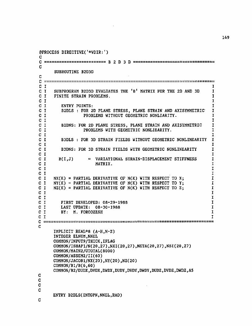
149
©PROCESS DIRECTIVE( '*VDIR: ' )CC ========================= B 2 D 3 D ==============================C
SUBROUTINE B2D3DCC = = = = = = = = = = = = = = = = = = = = = = = = = = = = = = = = = = = = = = = = = = = = = = = = = = = = = = = = = = = = = = = = = =
C IC I SUBPROGRAM B2D3D EVALUATES THE 'B 1 MATRIX FOR THE 2D AND 3DC I FINITE STRAIN PROBLEMS.C IC I ENTRY POINTS:C I B2DLS : FOR 2D PLANE STRESS, PLANE STRAIN AND AXISYMMETRIC’C I PROBLEMS WITHOUT GEOMETRIC NONLIARITY.C IC I B2DNS: FOR 2D PLANE STRESS, PLANE STRAIN AND AXISYMMETRICC I PROBLEMS WITH GEOMETRIC NONLIEARITY.C IC I B3DLS : FOR 3D STRAIN FIELDS WITHOUT GEOMETRIC NONLINEARITYC IC I B3DNS: FOR 3D STRAIN FIELDS WITH GEOMETRIC NONLINEARITYC IC l B ( I , J ) = VARIATIONAL STRAIN-DISPLACEMENT STIFFNESSC I MATRIX.C I C IC I NX(K) = PARTIAL DERIVATIVE OF N(K) WITH RESPECT TO X;C I NY(K) = PARTIAL DERIVATIVE OF N(K) WITH RESPECT TO Y;C I NZ(K) = PARTIAL DERIVATIVE OF N(K) WITH RESPECT TO Z;C I C IC I FIRST DEVELOPED: 08 -2 9 -1 9 8 8C I LAST UPDATE: 08 -3 0 -1 9 8 8C l BY: M. FOROOZESHC IC = = = = = = = = = = = = = = = = = = = = = = = = = = = = = = = = = = = = = = = = = = = = = = = = = = = = = = = = = = = = = = = = = = =
cIMPLICIT REAL*8 (A-H.N-Z)INTEGER ELNUM,NNEL COMMON/INPUT9/THICK,IFLAGCOMMON/ISHAP1/N(20,27),NXI(20,27),NETA(20,27),NSI(20,27) COMMON/MAIN2/UTOTALC 8000)COMMON/ASSEM2/II(60)COMMON/JACOB1/NX(20),NY(20),NZ(20)COMMON/B1/B(6,60)COMMON/B2/DUDX, DVDX,DWDX, DUDY, DVDY, DWDY, DUDZ, DVDZ, DWDZ, A5
CCCC
ENTRY B2DLS(INTGPN,NNEL,RAD)C

150
C CALCULATION OF THE <B> MATRIXCC*VDIR: ASSUME COUNT(8)
DO 100 K1 = l.NNEL K12 = 2*K1 K l l = K12 - 1 B (1 ,K 11) = NX(K1)B (1 ,K 12) = 0 .B (2 ,K 11) = 0 .B (2 ,K 12) = NY(K1)B (3 ,K 11) = NY(K1)B (3 ,K 12) = NX(K1)
100 CONTINUECC CALCULATION OF THE ADDITIONAL ROW OF <B> FOR THE AXISYM. CASE.C
IF (IFLAG.EQ.3) THENCC*VDIR: ASSUME C0UNT(8)
DO 200 K1 = 1 , NNEL K12 = 2*K1 K l l = K12 - 1B (4 ,K 11) = N(K1,INTGPN)/RAD
200 B (4 ,K 12) = 0 .C
END IFC
RETURNCCCC
ENTRY B2DNS(INTGPN,NNEL,RAD)CC ------ CALCULATION OF THE <B> MATRIXC
DUDX = 0 .DVDX = 0 .DUDY = 0 .DVDY = 0 .A5 = 0 .
C*VDIR: ASSUME C0UNT(8)DO 300 K1 = l.NNEL K12 = 2*K1 K l l = K12 - 1DUDX = DUDX + N X (K 1)*UT0TAL(II(K ll))DVDX = DVDX + NX(K1)*UT0TAL(II(K12))DUDY = DUDY + NY (K 1)*U T0T A L (II(K ll))DVDY = DVDY + NY(K1)*UT0TAL(II(K12))A5 = A5 + N(K1,INTGPN)*UT0TAL(II(K11))
300 CONTINUEC

C*VDIR: ASSUME C0UNT(8)DO 400 K1 = l.NNEL K12 = 2*K1 K ll = K12 - 1B (1 ,K11) = ( 1 . + DUDX)*NX(K1)B (1 ,K12) = DVDX*NX(K1)B(2,K 11) = DUDY*NY(K1)B(2,K 12) = ( 1 . + DVDY)*NY(K1)B (3 ,K11) = DUDY*NX(K1) + ( 1 . + DUDX)*NY(K1)B (3,K 12) = DVDX*NY( K1) + ( 1 . + DVDY)*NX(K1)
400 CONTINUECC ----- CALCULATION OF THE ADDITIONAL ROW OF <B> FOR THE AXISYM CASE.'C
IF (IFLAG.EQ.3) THEN AS = A5/RAD
CC*VDIR: ASSUME C0UNT(8)
DO 500 K1 = 1 , NNEL K12 = 2*K1 K ll = K12 - 1B(4 ,K 11) = (A5 + 1 . )*N(K1, INTGPN)/RAD
500 B (4,K 12) = 0 .C
END IFC
RETURNCCCC
ENTRY B3DLS(NNEL)CC - - - CALCULATION OF THE <B> MATRIX CC*VDIR: ASSUME COUNT(20) „
DO 600 K1 = l.NNEL K13 = 3*K1 K12 = K13 - 1 Kll = K13 - 2 B(1,K11) = NX(K1)B (1 ,K12) = 0 .B(1,K13) = 0.B(2,K11) = 0.B(2,K12) = NY(K1)BC2.K13) = 0.B(3,K11) = 0.B(3,K12) = 0.B(3,K13) = NZ(K1)B(4,K11) a NY(K1)BC4.K12) = NX(K1)B(4,K13) = 0.

B(5,K11) = 0 .B(5,K12) = NZ(K1)B(5,K13) = NY(K1)B(6,K11) = NZ(K1)B(6,K12) = 0 .B(6,K13) = NX(K1)CONTINUE
RETURNcccc
ENTRY B3DNS(NNEL)CC ---- CALCULATION OF THE <B> MATRIXC
DUDX = 0 .DVDX = 0 .DWDX = 0 .DUDY = 0 .DVDY = 0 .DWDY = 0.DUDZ = 0.DVDZ = 0.DWDZ = 0.
CC*VDIR: ASSUME C0UNT(20)
DO 700 K1 = l.NNEL K13 = 3*K1 K12 = K13 - 1 K ll = K13 - 2DUDX = DUDX + NX(K1)*UT0TAL(II(K11)) DVDX = DVDX + NX(K1)*UT0TAL(II(K12)) DWDX = DWDX + NX(K1)*UT0TAL(II(K13)) DUDY = DUDY + NY(K1)*UT0TAL(II(K11)) DVDY = DVDY + NY(K1)*UT0TAL(II(K12)) DWDY = DWDY + NY(K1)*UT0TAL(II(K13)) DUDZ = DUDZ + NZ(K1)*UT0TAL(II(K11)) DVDZ = DVDZ + NZ(K1)*UT0TAL(II(K12)) DWDZ = DWDZ + NZ(K1)*UT0TAL(II(K13))
700 CONTINUECC*VDIR: ASSUME COUNT(20)
DO 800 K1 = l.NNEL K13 = 3*K1 K12 = K13 - 1 K ll = K13 - 2B(1,K11) = ( 1 . + DUDX)*NX(K1)B(1.K12) = DVDX*NX(K1)B(1.K13) = DWDX*NX(K1)B(2,K11) = DUDY*NY(K1)

153
800C
C
B (2 ,K 12) = ( 1 . + DVDY)*NY(K1)B (2 ,K 13) = DWDY*NY(K1)B (3 ,K 11) = DUDZ*NZ(K1)B (3 ,K 12) = DVDZ*NZ(K1)B(3 ,K 13) = ( 1 . + DWDZ)*NZ(K1)B (4 ,K 11) = DUDY*NX(K1) + ( 1 . + DUDX)*NY(K1) B (4 ,K 12) = DVDX*NY(Kl) + ( 1 . + DVDY)*NX(K1) B (4 ,K 13) = DWDY*NX(Kl) + DWDX*NY(K1)B (5 ,K 11) - DUDZ*NY(K1) + DUDY*NZ(K1) B (5 ,K 12) = DVDZ*NY(K1) + ( 1 . + DVDY)*NZ(K1) B (5 ,K 13) = DWDY*NZ(K1) + ( 1 . + DWDZ)*NY(K1) B (6 ,K 11) = DUDZ*NX(K1) + ( 1 . + DUDX)*NZ(K1) B (6 ,K 12) = DVDX*NZ(K1) + DVDZ*NX(K1) B (6 ,K 13) = DWDX*NZ(K1) + ( 1 . + DWDZ)*NX(K1) CONTINUE
RETURN
END

n n
o154
^PROCESS DIRECTIVE( '*VDIR:' )
=================== A X I S Y M ==============
SUBROUTINE AXISYM( INTGPN, ELNUM, NNEL, RAD.THICK) CC = = = = = = = = = = = = = = = = = = = = = = = = = = = = = = = = = = = = = = = = = = = = = = = = = =
C IC I SUBPROGRAM AXISYM EVALUATES THE RADIUS OF THE INTEGRATIONC I POINT FROM THE AXIS OF SYMMETRY OF AXISYMMETRIC PROBLEMS.C I THE AXIS OF SYMMETRY IS ASSUMED TO BE THE Y AXIS.C IC I INTGPN = INTEGRATION POINT NUMBERC I ELNUM = ELEMENT NUMBERC I NNEL = NUMBER OF NODES IN THE ELEMENTC l RAD RADIUS OF THE INTEGRATION POINTC I THICK = SURCOMFRENCE OF THE AXISYMMETRIC SOLIDC IC I FIRST DEVELOPED: 09 -01-1988C I LAST UPDATE: 0 9 -01 -1988C l BY: M. FOROOZESHC = = = = = = = = = = = = = = = = = = = = = = = = = = = = = = = = = = = = = = = = = = = = = = = = = = = = = = = = = = = = = = = = =
REAL*8 RAD,THICK,N.NXI.NETA.NSI REAL*4 X.Y.Z INTEGER ELNUMCOMMON/ISHAP1/N(2 0 , 2 7 ) ,N X I(20, 2 7 ) ,NETA(20,2 7 ) ,N S I (2 0 ,2 7 ) COMMON/INPUT2/NOP(20,2000)COMMON/INPUT3/X(4000),Y(4000),Z(4000)
CRAD = 0 .
C*VDIR: ASSUME C0UNT(8)DO 10 K1 = 1 , NNELRAD = RAD + N(K1 , INTGPN)*X(N0P(K1 , ELNUM))
10 CONTINUEC
THICK = 6 . 283185307179586D0*RADC
RETURNEND

n n
n n
o n
nn
nn
nn
nn
nn
nn
nn
nn
nn
nn
n
on
(apROCESS DIRECTIVE( '*VDIR: ' )
====================== G E T S T R
SUBROUTINE GETSTR(IOUT)
II SUBROUTINE GETSTR ASSEMBELS THE GLOBAL STIFFNESS MATRIX AND/OR I STORES THE NODE NUMBERS OF THE CORENT ELEMENT AND THE POSITIONI OF THE ELEMENT MATRICES IN THE GLOBAL MATRICES.III I I ( J ) POSITION OF LOCAL STIFFNESS TERMS IN THE GLOBALI STIFFNESS MATRIX.II SKG(I) = GLOBAL STIFFNESS MATRIX IN THE CONDENSED FORMI S K (I ,J ) = ELEMENT STIFFNESS MATRIXI (SK IS COMPUTED BY SUBPROGRAM STIFEL)III FIRST DEVELOPED: 0 8 -2 6 -1 9 8 8I LAST UPDATE: 0 9 -0 5 -1 9 8 8I BY: M. FOROOZESH
IMPLICIT REAL*8 (A-H.O-Z)INTEGER ELNUMCOMMON/INPUT8/NNODES,NELEM, NNDF, NLINC, MNIT, IFLAG1, IFLAG2 , IDIM,
1 NINODECOMMON/INPUT9/THICK,IFLAG COMMON/INPUT1/NIPXI,NIPETA,NIPSI,NIP,INTCOD COMMON/INPUT2/NOP(2 0 ,2 0 0 0 )COMMON/ASSEM2/1 1 (6 0 )
NCB = NUMBER OF COLUMNS IN THE <B> MATRIX.NRB = NUMBER OF ROWS IN THE <B> MATRIX.NNEL = NUMBER OF NODES IN THE ELEMENT.
ITYPE1 = 0 IDENT1 = 0DO 80 ELNUM = 1 , NELEM
CALL ELINFOCELNUM, ITYPE, NNEL, IFLAG, ISTART,LINES)CALL ELINTM(ELNUM,IDENT,INTCOD,NIPXI,NIPETA,NIPSI,MATNUM,THICK) IF (ITYPE.NE.ITYPE1.OR.IDENT.NE.IDENT1) THEN
IF ( ITYPE.GT.300) THEN NCB = 3*NNEL NRB = 6IF ( INTCOD. GE.1 4 0 ) THEN
CALL ISH3DI(ITYPE,NNEL,IERROR)ELSE

CALL ISH3DG(ITYPE,NNEL,IERROR)END IF
ELSENCB = 2*NNELCALL ISH2DG(ITYPE, NNEL, IERROR)IF (IFLAG.EQ.3) THEN
NRB = 4ELSE
NRB = 3 END IF
END IF END IFITYPE1 = ITYPE IDENT1 = IDENT
CC*VDIR: PREFER SCALAR
DO 30 K1 = 1 , NNEL11 = NNDF*(K1 - 1)12 = NNDF*(N0P(K1 , ELNUM) - 1)
CC*VDIR: PREFER SCALAR
DO 30 K2 = 1 , NNDF K = I I + K2 I I ( K ) = 12 + K2
30 CONTINUECC GEOMETRICALLY NONLINEAR PROBLEMSC
IF (IFLAG1.EQ.1) THENIF(ITYPE.GT.300) THEN
CALL S3DNS (ELNUM,ITYPE,NNEL,NRB,NCB,NIP,MATNUM,IOUT)ELSE
CALL S2DNS (ELNUM,ITYPE,NNEL,NRB,NCB,NIP,MATNUM,IOUT) END IF
CC GEOMETRICALLY LINEAR PROBLEMSC
ELSE IF(IFLAGl.EQ.O) THEN IF(ITYPE.GT.300) THEN
CALL S3DLS (ELNUM,ITYPE,NNEL,NRB,NCB,NIP,MATNUM,IOUT)ELSE
CALL S2DLS (ELNUM,ITYPE,NNEL,NRB,NCB,NIP,MATNUM,IOUT) END IF
END IF • 80 CONTINUEC
100 RETURN END

no
n
^PROCESS DIRECTIVE('*VDIR:' )
:====================== E L S T R
SUBROUTINE ELSTR CuC I IC I SUBPROGRAM ELSTR EVALUATES THE STIFFNESS MATIRIX OF EACH ELEM. IC I IC I ENTRY POINTS: Ic I S2DLS : FOR 2D PLANE STRESS, PLANE STRAIN AND AXISYMMETRIC Ic I PROBLEMS WITHOUT GEOMETRIC NONLIARITY. Ic I Ic I S2DNS : FOR 2D PLANE STRESS, PLANE STRAIN AND AXISYMMETRIC Ic I PROBLEMS WITH GEOMETRIC NONLIEARITY. Ic I Ic I S3DLS : FOR 3D STRAIN FIELDS WITHOUT GEOM. NONLINEARITY Ic I Ic I S3DNS : FOR 3D STRAIN FIELDS WITH GEOMETRIC NONLINEARITY Ic I Ic I Ic I PARAMETER LIST: Ic I Ic I IFLAG = 1: PLANE STRAIN PROBLEM (ES2DLS ,ES2DNS ONLY) Ic I 2: PLANE STRESS PROBLEM (ES2DLS ,ES2DNS ONLY) Ic I 3: AXISYMMETRIC" PROBLEM (ES2DLS ,ES2DNS ONLY) Ic I Ic I ELNUM = ELEMENT NUMBER Ic I NNEL = NUMBER OF NODES IN THE ELEMENT Ic I NRB = NUMBER OF ROWS OF THE <B> MATRIX Ic I NCB = NUMBER OF COLUMNS OF THE <B> MATRIX Ic I NIP = TOTAL NUMBER OF INTEGRATION POINTS IN THE ELEM. Ic I IERROR = ERROR CODE Ic I Ic I Ic I FIRST DEVELOPED: 0 9 -0 1 -1 9 8 8 Ic I LAST UPDATE: 0 9 -0 2 -1 9 8 8 Ic I BY: M. FOROOZESH Icc
I I
CIMPLICIT REAL*8 (A-H.O-Z)REAL*8 N,NXI,NETA,NSI,NX,NY,NZ INTEGER ELNUM COMMON/ISHAP2/W(2 7 )COM M ON/ISHAP1/N(20,27),NXI(20,27),NETA(20,27),NSI(20,27)COMMON/MAIN2/UTOTAL(8000)COMMON/ASSEM2/II(6 0 )COMMON/JACOB1/NX( 2 0 ) , NY( 2 0 ) , NZ(2 0 )COMMON/B 2/DUDX, DVDX, DWDX, DUDY, DVDY, DWDY, DUDZ, DVDZ, DWDZ, A5 COMMON/INPUT9/THICK,IFLAG

C0MM0N/ELSTR1/STRN(6)CCCC
ENTRY S2DLS (ELNUM,ITYPE,NNEL,NRB,NCB,NIP,MATNUM,IOUT)C
DO 200 INTGPN = 1 , NIPCALL JACB2DCINTGPN, ELNUM, NNEL, IERROR,DETJAC) IF(IFLAG.EQ.3) CALL AXISYM(INTGPN,ELNUM,NNEL,RAD,THICK) CALL B2DLS(INTGPN,NNEL,RAD)CST = DETJAC*THICK*W( INTGPN )DUDX = 0 .DVDX = 0 .DUDY = 0 .DVDY = 0 .A5 = 0 .
C*VDIR: ASSUME C0UNT(8)DO 100 K1 = l.NNEL K12 = 2*K1 K ll = K12 - 1DUDX = DUDX + NX(K1)*UT0TAL(II(K11))DVDX = DVDX + NX(K1)*UT0TAL(II(K12))DUDY = DUDY + NY(K1)*UT0TAL(II(K11))DVDY = DVDY + NY(K1)*UT0TAL(II(K12))A5 = A5 + N(K1,INTGPN)*UT0TAL(II(K11))
100 CONTINUECC
STRN( 1 ) = DUDXSTRNC 2 ) = DVDYSTRN( 3 ) = DUDY + DVDXSTRNC 4 ) = 0 ,IF (IFLAG.EQ.3) STRNC 4 ) = A5/RAD
CCALL MATMODCELNUM, ITYPE, MATNUM, INTGPN, IFLAG, IOUT, DETJAC,1 ) CALL EQUILB(CST,NCB,NRB)
200 CONTINUEC
1000 RETURNCCCCCC
ENTRY S2DNS (ELNUM,ITYPE,NNEL,NRB,NCB,NIP,MATNUM,IOUT)C
DO 400 INTGPN = 1 , NIPCALL JACB2DCINTGPN, ELNUM, NNEL, IERROR, DETJAC)IF(IFLAG.EQ.3) CALL AXISYM(INTGPN,ELNUM,NNEL,RAD,THICK) CALL B2DNS(INTGPN,NNEL,RAD)

U U
U CJ
CJ CJ
CST = DETJAC*THICK*W( INTGPN )C
STRN( 1 ) = DUDX + 0.5*(DUDX**2 + DVDX**2 )STRN( 2 ) = DVDY + 0.5*(DUDY**2 + DVDY**2 )STRN( 3 ) = DUDY + DVDX + DUDX*DUDY + DVDX*DVDYSTRN( 4 ) = 0 .IF (IFLAG.EQ.3) STRN( 4 ) = A5 + 0 .5*(A 5**2)
CCALL MATMODCELNUM, ITYPE, MATNUM, INTGPN, IFLAG, IOUT .DETJAC, 1) CALL EQUILB(CST.NCB.NRB)
400 CONTINUEC
2000 RETURN
ENTRY S3DLS (ELNUM,ITYPE,NNEL,NRB.NCB,NIP,MATNUM,IOUT)C
DO 600 INTGPN = 1 , NIPCALL JACB3D(INTGPN, ELNUM, NNEL,IERROR,DETJAC)CALL B3DLS(NNEL)CST = DETJAC*W( INTGPN )
CDUDX = 0.DVDX = 0.DWDX = 0.DUDY = 0.DVDY = 0.DWDY = 0.DUDZ = 0.DVDZ = 0.DWDZ = 0.
CC*VDIR: ASSUME COUNT(20)
DO 500 K1 = l.NNEL K13 = 3*K1 K12 = K13 - 1 K ll = K13 - 2DUDX = DUDX + NX(K1)*UT0TAL(II(Kll))DVDX = DVDX + NX(K1)*UT0TAL(II(K12))DWDX = DWDX + NX(K1)*UT0TAL(II(K13))DUDY = DUDY + NY(K1)*UT0TAL(II(K11))DVDY = DVDY + NY(K1)*UT0TAL(II(K12))DWDY = DWDY + NY(K1)*UT0TAL(II(K13))DUDZ = DUDZ + NZ(K1)*UT0TAL(II(K11))DVDZ = DVDZ + NZ(K1)*UT0TAL(II(K12))DWDZ = DWDZ + NZ(K1)*UT0TAL(II(K13))
500 CONTINUEC
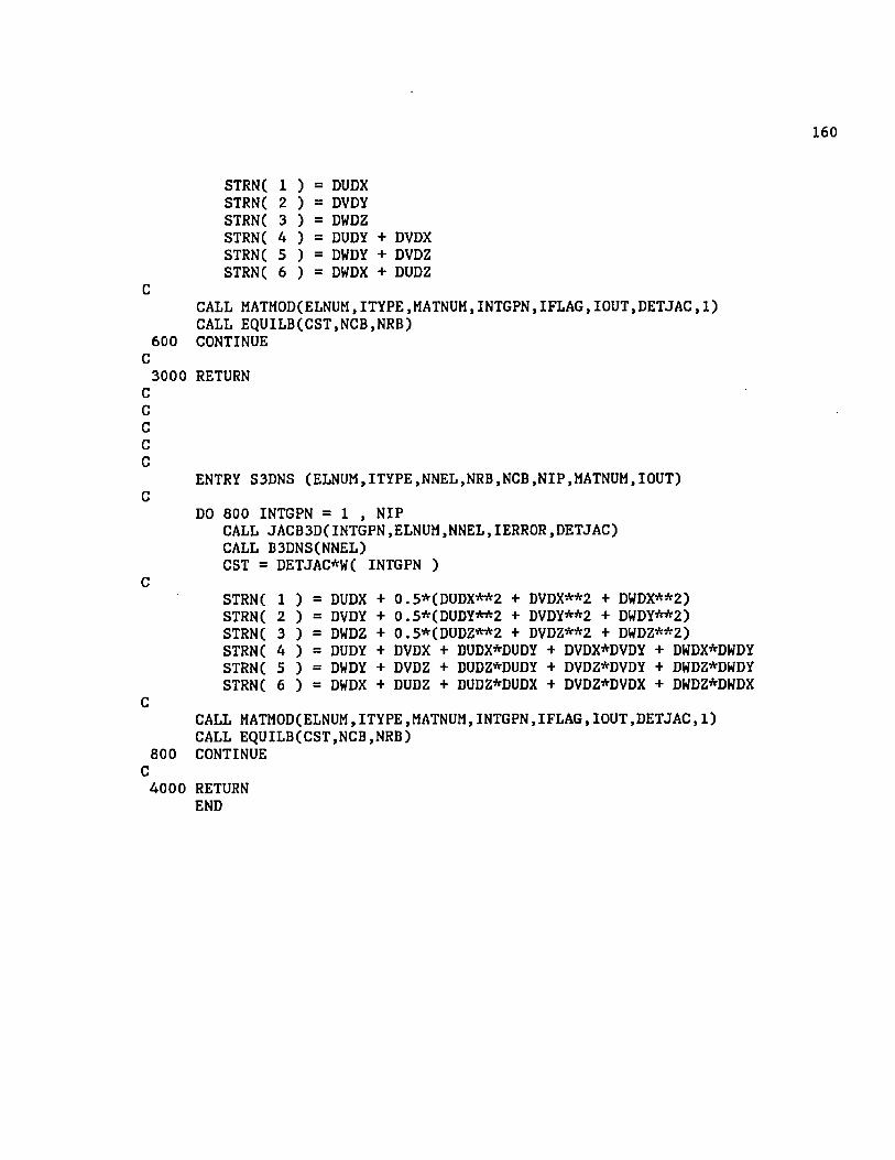
uo
ua
o
STRNC 1 ) = DUDXSTRNC 2 ) = DVDYSTRNC 3 ) = DWDZSTRNC 4 ) = DUDY + DVDXSTRNC 5 ) = DWDY + DVDZSTRNC 6 ) = DWDX + DUDZ
CALL MATMODCELNUM, ITYPE.MATNUM, INTGPN, IFLAG, IOUT,DETJAC, I ) CALL EQUILBCCST.NCB.NRB)
600 CONTINUE
3000 RETURN
ENTRY S3DNS CELNUM,ITYPE,NNEL,NRB,NCB,NIP,MATNUM,IOUT)C
DO 800 INTGPN = 1 , NIPCALL JACB3DCINTGPN, ELNUM, NNEL, IERROR, DETJAC)CALL B3DNSCNNEL)CST = DETJAC*WC INTGPN )
CSTRNC 1 ) = DUDX + 0.5*CDUDX**2 + DVDX**2 + DWDX**2)STRNC 2 ) = DVDY + 0.5*CDUDY**2 + DVDY**2 + DWDY**2)STRNC 3 ) = DWDZ + 0.5*CDUDZ**2 + DVDZ**2 + DWDZ**2)STRNC 4 ) = DUDY + DVDX + DUDX*DUDY + DVDX*DVDY + DWDX*DWDYSTRNC 5 ) = DWDY + DVDZ + DUDZ*DUDY + DVDZ*DVDY + DWDZ*DWDYSTRNC 6 ) = DWDX + DUDZ + DUDZ*DUDX + DVDZ*DVDX + DWDZ*DWDX
CCALL MATMODC ELNUM, ITYPE, MATNUM, INTGPN, IFLAG, IOUT, DETJAC,1 )CALL EQUILBCCST.NCB.NRB)
800 CONTINUEC
4000 RETURN END

^PROCESS DIRECTIVE( '*VDIR: ' )CC ========================= E Q U L I B =============C
SUBROUTINE EQUILBCCST.NCB.NRB)REAL*8 B, RE, STRESS, STRS, DS, CST, TEMP COMMON/ASSEM2/II(60)COMMON/ELSTR2/STRS(6 )COMMON/MAIN4/RE(8000)COMMON/B1/BC6.60)DIMENSION TEMPC60)
CC*VDIR: ASSUME COUNTC16)C*VDIR: IGNORE RECRDEPS
DO 200 K1 = 1 , NCB TEMP( K1 ) = 0 .DO 100 K2 = 1 , NRB
100 TEMP( K1 ) = TEMP( K1 ) + B(K2 , K1)*STRS( K2 ) 200 R ECII(K l)) = R E (II(K 1)) + TEMP( K1 )*CST
CRETURNEND

162
CC
^PROCESS DIRECTIVE( '*VDIR:' )CC ======================== C A U C H Y =============================C
SUBROUTINE CAUCHY(ELNUM, ITYPE,NNEL, NNDF, INTGPN, STRESS, CSTR) IMPLICIT REAL*8 (A-H.O-Z)REAL*8 NX.NY.NZ.JACMAT INTEGERS ELNUMCOMMON/JACOB1/NX(2 0 ) ,NY (20),N Z(20)COMMON/MAIN2/UTOTAL(8000)COMMON/INPUT2/NOP(20,2000)
CDIMENSION JACMAT(3 , 3 ) , PIOLA(3 , 3 ) , CAUCH( 3 , 3 ) , STRESS( 6 ) , CSTR(6 )
DUDXDUDYDUDZDVDXDVDYDVDZDWDXDWDYDWDZ
0.0.0.0.0.0 .0 .0 .0 .
IF ( ITYPE.GT.300) THENCALL JACB3D(INTGPN, ELNUM, NNEL, IERROR, DETJAC)
CC*VDIR:
10
ASSUME COUNT(20)DO 10 K1 = 1 , NNEL K ll = NNDF*(N0P(K1 , K12 = K ll + 1
ELNUM) - 1) + 1
K13 == K ll + 2DUDX = DUDX + NX( K1 )*UTOTAL( K ll )DUDY = DUDY + NY( K1 )*UTOTAL( K ll )DUDZ = DUDZ + NZ( K1 )*UTOTAL( K ll )DVDX = DVDX + NX( K1 )*UTOTAL( K12 )DVDY = DVDY + NY( K1 )*UTOTAL( K12 )DVDZ = DVDZ + NZ( K1 )*UTOTAL( K12 )DWDX = DWDX + NX( K1 )*UTOTAL( K13 )DWDY = DWDY + NY( K1 )*UTOTAL( K13 )DWDZ = DWDZ + NZ( K1 )*UTOTAL( K13 )CONTINUE
PIOLA(lPIOLA(2PI0LA(3PIOLA(lPI0LA(2PIOLA(lPIOLA(3PIOLA(2
1)2)3)2)1)3)1)3)
STRESS( STRESS( STRESS( STRESS( STRESS( STRESS( STRESS( STRESS(

PIO LA (3 , 2 ) = STRESSC 5 )ELSE
CALL JACB2DCINTGPN.ELNUM, NNEL, IERROR, DETJAC)CC*VDIR: ASSUME COUNT(8)
DO 20 K1 = 1 , NNELK ll = NNDF*(N0P(K1 , ELNUM) - 1) + 1K12 = K l l + 1DUDX = DUDX + NX( K1 )*UTOTAL( K l l )DUDY = DUDY + NY( K1 )*UTOTAL( K l l )DVDX = DVDX + NX( K1 )*UTOTAL( K12 )DVDY = DVDY + NY( K1 )*UTOTAL( K12 )
20 CONTINUEC
PIOLAfl J 1) = STRESSC 1 )PI0LAC2 9 2) = STRESSC 2 )PIOLAC1 I 2) = STRESSC 3 )PI0LAC2 9 1) = STRESSC 3 )PIOLA(3 9 3) = STRESSC 4 )PIOLA(1 9 3) = 0 .
PIOLA(2 9 3) = 0 .
PIOLA(3 9 1) = 0 .
PIOLA(3 9 2) = 0 .
END IFC
JACMAT(1 , 1) = 1. + DUDXJACMAT(1 , 2 ) = DUDYJACMAT(1 , 3 ) = DUDZJACMAT(2 , 1) = DVDXJACMATC2 , 2) = 1. + DVDYJACMAT(2 , 3) = DVDZJACMAT(3 , 1) = DWDXJACMAT(3 , 2 ) = DWDYJACMAT(3 , 3 ) = 1. + DWDZ
CDJAC = ( 1 . + DUDX)*((1. + DVDY)*(1. + DWDZ) - DVDZ*DWDY) -
1 DUDY*( DVDX*( 1 . + DWDZ) - DVDZ*DWDX) +2 DUDZ*(DVDX*DWDY - ( 1 . + DVDY)*DWDX)
CC*VDIR: PREFER SCALAR
DO 40 K1 = 1 , 3 C*VDIR: PREFER SCALAR
DO 40 K2 = 1 , K1 SUM = 0 .
C*VDIR: PREFER SCALAR DO 30 K3 = 1 , 3
C*VDIR: PREFER SCALAR DO 30 K4 = 1 , 3
30 SUM = SUM + PI0LACK3 , K4)*JACMAT(K1 , K3)*JACMAT(K2 , K4) 40 CAUCH(K1 , K2) = SUM/DJAC
CIF ( ITYPE.GT.300) THEN

164
CSTR( 1 ) = CAUCH(1 % 1)CSTR( 2 ) = CAUCH(2 i 2)CSTR( 3 ) = CAUCH(3 9 3)CSTR( 4 ) = CAUCH(2 9 1)CSTR( 5 ) = CAUCHC3 9 2)CSTR( 6 ) CAUCH(3 9 1)
CSTR( 1 ) = CAUCH(1 9 1)CSTR( 2 ) = CAUCH(2 9 2)CSTR( 3 ) = CAUCH(2 9 1)CSTR( 4 ) = CAUCH(3 9 3)
END IFC
RETURNEND

165
©PROCESS DIRECTIVE(’*VDIR:1)CC = = = = = = = = = = = = = = = = = = = = = = = = = = = G L O B A L = = = = = = = = = = = = = = = = = = = = = = = = = =C
SUBROUTINE GLOBALCC ==================================================================C IC I SUBROUTINE GLOBAL IS USED TO MODIFY THE FINAL GLOBALC I STIFFNESS MATRIX. THIS IS DONE IN ORDER TO SOLVE THEC I SET OF SIMULTINOUS EQUATIONS BY THE METHOD OF MODIFFICATION.C I THIS SUBROUTINE IS DESIGED FOR MODIFICATION OF BANDEDC I NONSYMETRIC MATRICES IN THEIR CONDENSED FORM.C I C IC ==================================================================C
IMPLICIT REAL*8 (A-H.O-Z)DIMENSION IDOF( 1 )
CCC E N T R Y G L O B 1C
ENTRY GLOB1(NNODES, NNDF, NTDF, IDOF)C
MDOF = NNDF*NNODES ICOUNT = 0
CC*VDIR: PREFER SCALAR
DO 40 ID = 1 , MDOF IF (IDOF( ID ) . EQ.0 ) THEN
ICOUNT = ICOUNT + 1 IDOF( ID ) = ICOUNT
ELSE IF (IDOF( ID ) .G T .O ) THEN IDOF( ID ) = 0
END IF 40 CONTINUE
NTDF = ICOUNTC
RETURNCCC E N T R Y G L 0 B 2C
ENTRY GL0B2(NN0DES,NNDF,NTDF,IDOF)C
MDOF = NNDF*NNODES ICOUNT = 0
CC*VDIR: PREFER SCALAR
DO 50 ID = 1 , MDOF IF (IDOFC ID ) .GT.O) THEN

ICOUNT = ICOUNT + 1 IDOF( ID ) = ICOUNT
END IF CONTINUE NTDF = ICOUNT
RETURNEND

no
n
©PROCESS DIRECTIVE( r*VDIR:1)
D I A G N L
SUBROUTINE DIAGNL(NELEM, NNDF, NTDF, IDOF, JDIAG, NTSK, MBAND, IFLAG2, 1 IOUT)
cc I Ic I THIS PROGRAM COMPUTES THE VECTOR CONTAINING THE ADDRESSES Ic I OF THE DIAGNAL ELEMENTS OF THE STIFFNESS MATIX. IT ALSO Ic I CALCULATES THE BANDWIDTH AND THE AVERAGE BANDWIDTH OF THE Ic I OF THE STIFFNESS MATRIX AND PRINTS THESE STATISTICS. Ic I Tc I A R G U M E N T L I S T Ic I Ic I . NELEM = TOTAL NUMBER OF ELEMENTS Ic I Ic I NNDF = NUMBER OF NODAL DEGREES OF FREEDOM Ic I Ic I NTDF = NUMBER OF TOTAL DEGREES OF FREEDOM Ic I Ic I IDOF(I) = VECTOR CONTAINING THE D.O.F. NUMBERS OF THE NODES Ic I Ic I JDIAG(I) = VECTOR CONTAINING THE ADDRESS OF THE DIAGNAL TERMS Ic I IN THE GLOBAL STIFFNESS MATRIX 'SKG1 Ic I Ic I NTSK = NUMBER OF TERMS IN THE GLOBAL STIFFNESS MATRIX Ic I Ic I MBAND = HALF BANDWIDTH OF THE STIFFNESS MATRIX Ic I Ic I IOUT = OUTPUT DEVICE NUMBER Ic I Ic I Ic I C 0 M M 0 N B L O C K S Ic I Ic I NOP(I,J) = MEMBER INCIDENCES Ic I Ic I Icc
I I
INTEGER ELNUMCOMMON/INPUT2/NOP(2 0 ,2 0 0 0 )DIMENSION ID 0F (1 ) , JDIAG(l)
CMBAV = 0 MBAND = 0
C*VDIR: PREFER VECTORDO 5 K = 1 , NTDF
5 JDIAG( K ) = 0C
DO 30 ELNUM = 1 , NELEMCALL ELINFO(ELNUM,ITYPE,NNEL,IFLAG, ISTART,LINES)

no
on
n
oo
n
non
n
on168
MAXDOF = 0MINDOF = 1000000DO 20 NODE = 1 , NNEL DO 20 IDIR = 1 , NNDF K = NNDF*(N0P(N0DE , ELNUM)- - 1) + IDIR IF(ID 0F( K ) ) 2 0 , 2 0 , 1 0
10 MAXDOF = MAX0(MAXDOF , ID0F( K ) )MINDOF = MIN0(MINDOF , IDOF( K ) )
20 CONTINUE
AT THIS POINT THE HIGHT OF EACH COLUMN IS STORED IN JDIAG
DO 26 NODE = 1 , NNEL DO 26 IDIR = 1 , NNDFID = NNDF*(NOP(NODE , ELNUM) - 1) + IDIR ID = ID0F( ID )IF ( ID )26 , 26 , 25
25 MHT = ID - MINDOF + 1IF(MHT.GT.JDIAG( ID ) ) JDIAG( ID ) = MHT
26 CONTINUE
FIND THE BANDWIDTH AND THE AVERAGE BANDWIDTH
MBN = MAXDOF - MINDOF MBAND = MAXO(MBAND , MBN)MBAV = MBAV + MBAND
30 CONTINUE
MBAV = MBAV/NELEM + 1 MBAND = MBAND + 1
LOCATION OF EACH DIAGNAL TERM WILL NOW BE STORED IN JDIAG
IF (IFLAG2.EQ.0) THEN MHT = 1 ID = 0DO 40 K = 1 , NTDF+1 ID = ID + MHT MHT = JDIAG( K )
40 JDIAG( K ) = IDNTSK = JDIAG(NTDF+1) - JDIAG( 1 )
ELSEID = 0DO 50 K = 1 , NTDF ID = ID + JDIAG( K )
50 JDIAG( K ) = IDNTSK = 2*JDIAG( NTDF )
END IF
NTSK = NUMBER OF TERMS IN THE GLOBAL STIFFNESS MATRIX "SKG"

169
WRITE(IOUT , 100)NTDF,MBAND,MBAV,NTSK 100 FORMATC//IX,'NUMBER OF EQUATIONS = ' , I 8 /1 X , 'HALF BANDWIDTH = ' ,
1 I 8 / I X , ’AVERAGE BANDWIDTH = 1, I 8 /1 X , 'S I Z E OF THE STIFFNESS MATRIX'2 , ' = ' , 1 8 )
RETURNEND
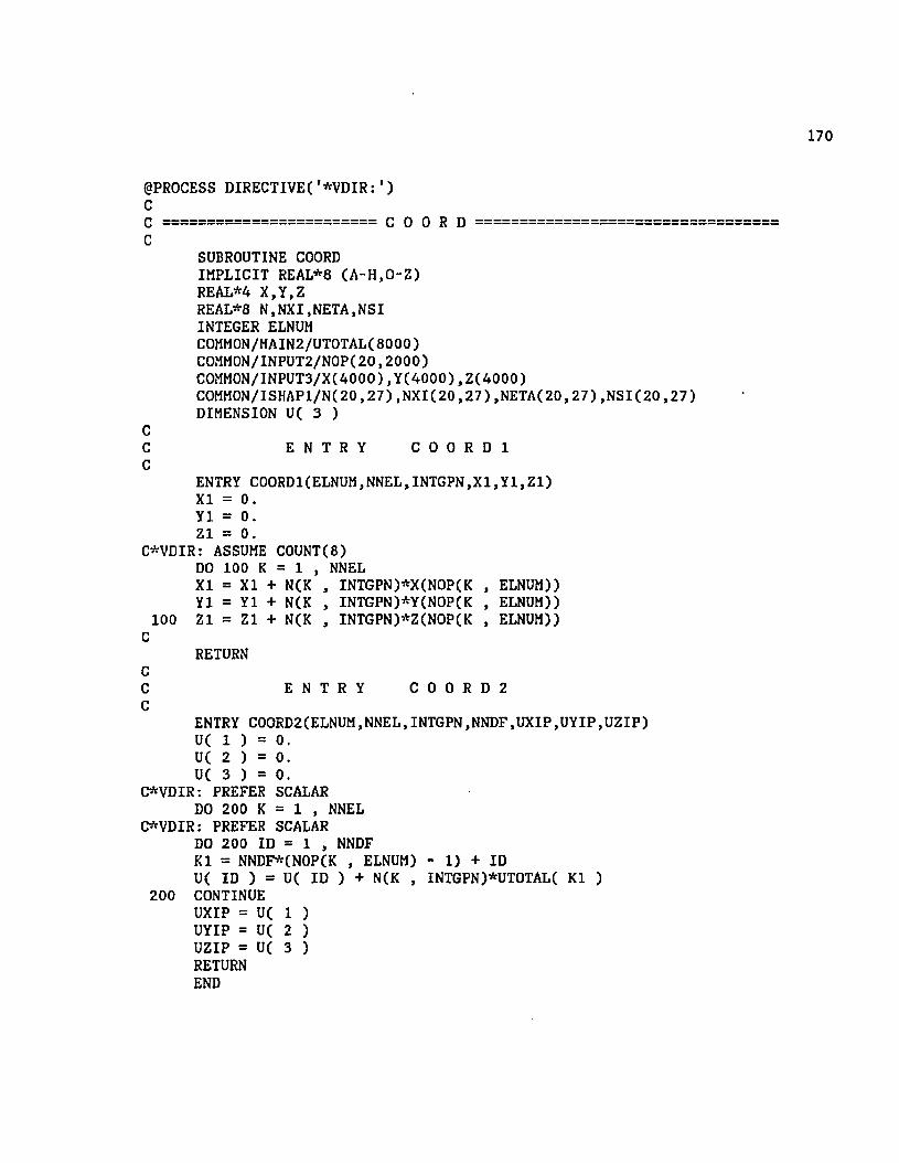
©PROCESS DIRECTIVE(’*VDIR: ' )CC ======================== C O O R D =========================C
SUBROUTINE COORD IMPLICIT REAL*8 (A-H.O-Z)REAL*4 X,Y,Z REAL*8 N,NXI,NETA,NSI INTEGER ELNUM COMMON/MAIN2/UTOTAL(8000)COMMON/INPUT2/N0PC 2 0 ,2 0 0 0 ) COMM0N/INPUT3/X(4000),Y(4000),Z(4000)COMMON/ISHAP1/N(2 0 , 2 7 ) ,N X I(2 0 ,2 7 ) ,N E T A (2 0 ,2 7 ) ,N S I (2 0 ,2 7 ) DIMENSION U( 3 )
CC E N T R Y C 0 0 R D 1C
ENTRY COORD1 (ELNUM, NNEL, INTGPN, X1 , Y1 , Z1)XI = 0 .Y1 = 0 .Z1 = 0 .
C*VDIR: ASSUME C0UNT(8)DO 100 K = 1 , NNELXI = XI + N(K , INTGPN)*X(NOP(K , ELNUM))Y1 = Y1 + N(K , INTGPN) *Y(NOP( K , ELNUM))
100 Z1 = Z1 + N(K , INTGPN)*Z(NOP(K , ELNUM))C
RETURNCC E N T R Y C 0 0 R D 2C
ENTRY COORD2( ELNUM, NNEL, INTGPN, NNDF,UXIP,UYIP,UZIP)U( 1 ) = 0 .U( 2 ) = 0 .U( 3 ) = 0 .
C*VDIR: PREFER SCALARDO 200 K = 1 , NNEL
C*VDIR: PREFER SCALARDO 200 ID = 1 , NNDFK1 = NNDF*(NOP(K , ELNUM) - 1) + IDU( ID ) = U( ID ) + N(K , INTGPN)*UTOTAL( K1 )
200 CONTINUEUXIP = U( 1 )UYIP = U( 2 )UZIP = U( 3 )RETURNEND

no
n
@PROCESS DIRECT!VE('*VDIR:')
====================== H A T M O D =============================
SUBROUTINE MATMOD(ELNUM, ITYPE, MATNUM, INTGPN, IFLAG, IOUT.DETJAC, it ICODE)
IMPLICIT REAL*8 (A-H.O-Z)INTEGER ELNUM COMMON/ INPUTF/MATYPE( 1 0 )
CI = MATYPE( MATNUM )IF ( I . E Q . l ) THEN
CALL ELAST(ITYPE,MATNUM,IFLAG,IOUT,ICODE)ELSE IF C I.E Q .2) THEN
CALL PLASTN(ELNUM, ITYPE,MATNUM, INTGPN, IFLAG, IOUT,DETJAC, it ICODE)
ELSE I F ( I .E Q .3 ) THENCALL PLASTL(ELNUM, ITYPE.MATNUM, INTGPN, IFLAG, IOUT.DETJAC,
it ICODE)ELSE
WRITE (IOUT , 100) I STOP
END IFC
RETURN100 FORMAT (/IX ,'IN V A L ID MATERIAL T Y P E ( ' , I 3 , ' ) SPECIFIED')
END

o o
n o
n n
nn
nn
nn
nn
nn
nn
oo
on
no
oo
oo
n
n o
APPENDIX B
SOLVER MODULE
====================== S 0 L V E 1 =========
SUBROUTINE SOLVEl(A,C,B,JDIAG,NEQ.AFAC,BACK)
II P R O G R A M :II PROGRAM ' SOLVE1 1 IS USED TO SOLVE A SERIES OF BANDED I NONSYMETRIC LINEAR EQUATIONS USING THE GAUSS ELIMINATION/BACK I SUBSTITUTION WITH NO COLUMN PIVOTING.II STORAGE:I I I I I I II LAST UPDATE: 12-30 -1988I BY: M. FOROOZESHI
IMPLICIT REAL*8 (A-H.O-Z)LOGICAL AFAC,BACKDIMENSION A( 1 ) ,C ( 1 ) ,B ( 1 ),JDIAG( 1 )
FACTOR A TO UT*D*U, REDUCE B TO Y
JR = 0DO 300 J = 1 , NEQ JD = JDIAG( J )JH = JD - JR IF (J H .L E .l) GO TO 300 IS = J + 1 - JH IE = J - 1IF ( .NOT.AFAC) GO TO 250 K = JR + 1 ID = 0
REDUCE ALL EQUATIONS EXCEPT DIAGNAL
DO 200 I - IS , IE IR = ID
COEFICIANT MATRIX SHOULD BE STORED IN TWO ONE DIMENSIONAL ARRAYS USING THE SKYLINE OR THE PROFILE METHODA( K ) = UPPER TRIANGULAR MATRIXC( K ) = LOWER TRIANGULAR MATRICB( K ) = RIGHT HAND SIDE VECTOR ON CALL
= VECTOR OF UNKNOWNS ON RETURN
172

ID = JDIAG( I )IH = MIN0(ID-IR-1 , I - IS )IF (IH.EQ.O) GO TO 150A( K ) = A( K ) - DOTPRO(A( K-IH ) ,C( ID-IH ) , I H )C( K ) = C( K ) - DOTPRO(C( K-IH ) ,A ( ID-IH ) , I H )
150 IF (A(ID ).NE.O .O ) C( K ) = C( K ) /A ( ID )200 K = K + 1
CC REDUCE THE DIAGNAL TERMC
A( JD ) = A( JD ) - DOTPRO(A( JR+1 ) ,C ( JR+1 ) ,J H - 1 )CC FORWARD REDUCE THE RIGHT HAND SIDEC
250 IF ( BACK ) B( J ) = B( J ) - DOTPRO(C( JR+1 ) ,B ( IS ) ,J H - 1 )300 JR = JD
IF(.NOT.BACK) RETURNCC BACK SUBSTITUTIONC
J = NEQJD = JDIAG( J )
500 IF (A( JD ) .N E .0 .0 ) B( J ) = B( J ) /A ( JD )D = B( J )J = J - 1 IF (J .L E .O ) RETURN JR = JDIAG( J )IF (JD -JR .L E .1) GO TO 700 IS = J - JD + JR + 2K = JR - IS + 1DO 600 I = IS , J
600 B( I ) = B( I ) - A( I+K )*D700 JD = JR
GO TO 500 END
C
CFUNCTION DOTPRO(A,B,N)REAL*8 A, B , DOTPRO, TEMP DIMENSION A( 1 ) , B( 1 )TEMP = 0 .0 DO 100 I = 1 , N
100 TEMP = TEMP + A( I )*B( I )DOTPRO = TEMP
CRETURNEND

174
Cc ========================== s 0 L V E 2 ===========================C
SUBROUTINE SOLVE2(A,R, JDIAG,NEQU.KKK,IOUT)CC ==================================================================C IC I THIS PROGRAM IS USED TO SOLVE FINITE ELEMENT STATIC EQUILIB.C I EQUATIONS IN CORE, USING COMPACTED STORAGE AND COLUMN REDUCTONC I SCHEME C IC ==================================================================c
IMPLICIT REAL*8(A-H,0-Z)DIMENSION A( 1 ) , JDIAG( 1 ) , R( 1 )
CC PERFORM L*D*L FACTORIZATION OF THE STIFFNESS MATRIXC
IF (KKK - 2) 40 , 150 , 15040 DO 140 N = 1 , NEQU
KN = JDIAG( N )KL = KN + 1 KU = JDIAG(N+l) - 1 KH = KU - KL IF (KH) 1 1 0 ,9 0 ,5 0
50 K = N - KHIC = 0 KLT = KUDO 80 J = 1 , KH IC = IC + 1 KLT = KLT - 1 KI = JDIAGC K )ND = JDIAGC K + 1 ) - KI - 1 IF (ND) 80 , 80 , 60
60 KK = MIN0(IC,ND)C = 0 .DO 70 L = 1 , KK
70 C = C + A(KI + L)*A(KLT + L)A( KLT ) = A( KLT ) - C
80 K = K + 190 K = N
B = 0 .DO 100 KK = KL , KUK = K - 1KI = JDIAGC K )C = A( KK ) / A( KI )B = B + C*A( KK )
100 A( KK ) = CA( KN ) = A( KN ) - B
110 IF (A( KN ) ) 120 ,120 , 140120 WRITE(IOUT , 2000) N , A( KN )
STOP

140 CONTINUERETURN
CC REDUCE THE RIGHT-HAND-SIDE LOAD VECTORC
150 DO 180 N = 1 , NEQU KL = JDIAGC N ) + 1KU = JDIAGC N + 1) - 1IFCKU-KL) 180 , 160 , 160
160 K = NC = 0 .DO 170 KK = KL , KU K = K - 1
170 C = C + AC KK )*RC K )RC N ) = RC N ) - C
180 CONTINUECC BACK-SUBSTITUTEC
DO 200 N = 1 , NEQU K = JDIAGC N )
200 RC N ) = RC N ) / AC K )C
IF CNEQU.EQ.l) RETURN N = NEQUDO 230 L = 2 , NEQU KL = JDIAGC N ) + 1KU = JDIAGC N + 1 ) - 1IF C KU - KL ) 230 , 210 , 210
210 K = NDO 220 KK = KL , KU K = K - 1
220 RC K ) = RC K ) - AC KK )*RC N )230 N = N - 1
RETURN2000 F0RMATC//1X,'STOP - STIFFNESS MATRIX NOT POSITIVE DEFINITE ’ / /
1 IX ,' NONPOSITIVE PIVOT FOR EQUATION ' , 1 4 / / IX,'PIVOT = ' ,E 2 0 .1 2 )END

APPENDIX C
PLASTICITY MODULE
SUBROUTINE PLAST(ELNUM, ITYPE, MATNUMt INTGPN, IFLAG, IOUT, ICODE)CC ================================================================C IC l P R O G R A M :C IC I 'PLAST' IS ENTRANCE POINT TO THE PLASTICITY MODULE.C I DEPENDING ON THE VALUE OF "ICODE" THIS ROUTINE PERFORMSC I THE FOLLOWING FUNCTIONS.C IC l 1) ICODE = 1; CALLS SUBROUTINE 'MISESl' FOR EVALUATIONC l OF THE ELASTO-PLASTIC STIFFNESS TENSOR.C l 2) ICODE = 2; CALLS SUBROUTINE 'MISES21 FOR EVALUATIONC l OF THE STRESSES, PLASTIC STRAINS, ETC.C IC l A R G U M E N T L I S T S :C IC I ELNUM = ELEMENT NUMBERC I ITYPE = ELEMENT TYPEC I MATNUM = MATERIAL NUMBERC I INTGPN = INTEGRATION POINT NUMBERC I IFLAG = ANALYSIS TYPE CODEC l X; PLANE STRESSC l 2 ; PLANE STRAINC l 3; AXISYMMETRICC I IOUT = OUTPUT DEVICE NUMBERC I ICODE = TASK DEFINITION CODE AS DEFINED ABOVE.C IC ===============================================================
INTEGER ELNUMC
IF(ITYPE.GT.300) THEN IEND = 6
ELSEIEND = 4
END IFC
IF ( ICODE.EQ.O) THENCALL MISESl(ELNUM,ITYPE,MATNUM.INTGPN,IFLAG,IOUT,IEND)
ELSECALL MISES2(ELNUM, ITYPE, MATNUM, INTGPN, IFLAG, IOUT, IEND)
END IF RETURN END
176

u u
o
177
==================== M I S E S
SUBROUTINE MISEScnuc Ic I p R 0 G R A M:c Ic I 'MISES t IS THE CONTROL UNIT FOR:c Ic I 1) EVALUATION OF THE STRESS-STRAIN STIFFNESS MATRIXc I 2) CALCULATION OF THE STRESSES, PLASTIC STRAINS,c I PLASTIC WORK, AND THE SHIFT STRESS TENSOR.c Ic I E N T R Y P O I N T S :c Ic I MISESl: EVALUATES THE STRESS-STRAIN STIFFNESS MATRIXc I MISES2: EVALUATES THE STRESSES, STRAINS, ETC.c Ic I A R G U M E N T L I S T S :c Ic I ELNUM = ELEMENT NUMBERc I ITYPE = ELEMENT TYPEc I MATNUM = MATERIAL NUMBERc I INTGPN = INTEGRATION POINT NUMBERc I IFLAG = ANALYSIS TYPE CODEc I 1; PLANE STRESSc I 2; PLANE STRAINc I 3; AXISYMMETRICc I IOUT = OUTPUT DEVICE NUMBERc I IEND = 4; PLANE STRESS, PLANE STRAIN AND AXISYMMETRICc I = 6; 3-Dc Icn
IL»c
IMPLICIT REAL*8 (A-H ,0-Z)REAL*8 NUX,NUY,NUZ CHARACTER*1 IYIELD,IY INTEGER ELNUM COMMON/MEMO/MATAD,MATDE COMMON/TEMP/PRESS, PLWORK COMMON/ISHAP2/W(27)COMMON/DEVICE/LDEV1 ,LDEV2, LDEV3, LDEV4,LDEV5, LDKEEP, LDEV, LDEVST COMMON/UTILl/STRESS(6),STRAIN(6),STRELA(6),CENTER(6), WORK,IYIELD COMMON/CONTRl/INCREM.NIT COMMON/ELSTRl/STRN(6)C0MM0N/ELSTR2/STRS(6)COMMON/ADMATl/AD(9,9 )COMMON/PLAST1/IYIEL(2000)COMMON/FDER1/FJ, FK, FS(9 ) , FE( 9 ) , FZ(9 )

cccccccc
c cc ---c
200cc --- c
cc — c
cc -c
178
COMMON/MATERl/DEP(6,6)COMMON/ELPLDl/DEPM(9 , 9 ) ,ALAM(9),AMU(9)COMMON/INPUT8/NNODES, NELEM, NNDF, NLINC,MNIT, IFLAG1 , IFLAG2 , IDIM,
1 NINODECOMMON/INPUT5/NUX(10),NUY(1 0 ) ,NUZ(1 0 ) ,EX (1 0 ) ,EY (1 0 ) ,E Z (1 0 ) ,P 1X (10
1 ,P 1 Y (1 0 ),P 1 Z (1 0 ),P 2 X (1 0 ),P 2 Y (1 0 ),P 2 Z (1 0 )DIMENSION S 0 (9 ) ,C (9 ) ,Z (9 ) ,R R (9 ) ,E (9 ) ,D E L (9 ) ,E D (9 ) ,
1 ED0T(9),SF(9),EDOTEL(9),EDOTPL(9),DELAS(6),DE(6),SDOT(9
DATA D E L / l . , 0 . , 0 . , 0 . , l . , 0 . , 0 . , 0 . , l . /
E N T R Y M I S E S l
ENTRY MISES1(ELNUM, ITYPE, MATNUM, INTGPN, IFLAG, IOUT, IEND)
IYIELD = 1 'IF (INCREM.GT.1) THEN
CALL IOGET(LDEV,201,'(A201)',6 )CALL IOBKS(LDEV)
END IF
IF ( IYIELD.EQ.’Y1) THEN
CALCULATION OF THE USEFUL MATRICES
CALL TENSORCITYPE,STRESS,SO,1 . )CALL TENSOR(ITYPE,STRAIN,E,0. 5 )CALL TENSOR( ITYPE, CENTER, Z, 1 . )DO 200 KI = 1 , 9C( KI ) = 2 .*E ( KI ) + DEL( KI )
GET THE MATERIAL PARAMETERS
C3 = P1Y( MATNUM )SY = P1Z( MATNUM )BETA = P1X( MATNUM )YOUNG = EX( MATNUM )POISS = NUX( MATNUM )
CALCULATION OF THE FOURTH ORDER ELASTIC STIFFNESS MATRIX
IF ( MATNUM.NE.MATAD) THENCALL ADMAT(YOUNG,POISS)MATAD = MATNUM
END IF
CALCULATION OF THE JACOBIAN OF DEFORMATION
CALL DEFJAC(E,DEL,RR,DJAC)

179
CC ----- CALCULATION OF THE YIELD FUNCTIONC
CALL YIELD(S0,C,Z,W0RK,DJAC,C3,SY,F,F1,F2)CC ----- CALCULATION OF THE PARTIAL DERIVATIVE OF THE YIELD FUNCTIONC - - - F WITH RESPECT TO THE <STRESS>,<STRAIN>, THE JACOBIAN.C
CALL FDER(S0,C, Z ,DJAC,F1,F2,C3)CC - - - CALCULATION OF THE ELASTOPLASTIC STIFFNESS MATRIX C
CALL ELPLD( SO, Z , RR, DJAC, BETA, DEN,0 )CC ----- CONVERTION OF THE FORTH ORDER STIFFNESS TENSOR TO A SECONDC - - - ORDER TENSOR C
CALL CONVER(DEPM, DEP, IFLAG, ITYPE)ELSE
CALL DELAST(ITYPE.MATNUM,IFLAG)END IF RETURN
CCCCC E N T R Y M I S E S 2C
ENTRY MISES2(ELNUM, ITYPE, MATNUM, INTGPN, IFLAG, IOUT, IEND)C
FACTOR = 1.FACSUM = 0 .
CIF (INCREM.GT.1) THEN
CALL I0GET(LDEV1, 2 0 1 , ' (A 2 0 1 )1,6 )ELSE
DO 10 KI = 1 , IEND STRAINC KI ) = 0 .STRESS( KI ) = 0 .CENTER( KI ) = 0 .
10 STRELAC KI ) = 0 .WORK = 0 .
END IFCC ----- CALCULATION OF THE STRAIN INCREMENTC
DO 20 KI = 1 , IEND20 DE( KI ) = STRN( KI ) - STRAIN( KI )
CC ----- CALCULATION OF THE USEFULL TENSORSC
CALL TENSOR(ITYPE,STRESS,SO,1 . )
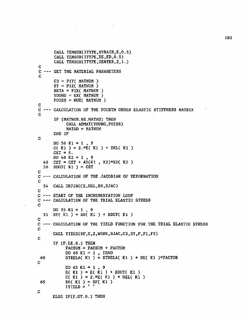
oo
o
Qo
oo
no
n
o n
on
n
no
160
CALL TENSOR(ITYPE,STRAIN,E,0 . 5 )CALL TENSOR( ITYPE,DE,ED,0 . 5 )CALL TENSORCITYPE, CENTER, Z , 1 . )
GET THE MATERIAL PARAMETERS
C3 = P1Y( MATNUM )SY = P1Z( MATNUM )BETA = P1X( MATNUM )YOUNG = EX( MATNUM )POISS = NUX( MATNUM )
- - - CALCULATION OF THE FOURTH ORDER ELASTIC STIFFNESS MATRIX
IF ( MATNUM.NE.MATAD) THENCALL ADMAT(YOUNG,POISS)MATAD = MATNUM
END IF
DO 50 KI = 1 , 9C( KI ) = 2 .*E ( KI ) + DEL( KI )CST = 0 .DO 40 K2 = 1 , 9
40 CST = CST + AD(K1 , K2)*ED( K2 )50 SD0T( KI ) = CST
— CALCULATION OF THE JACOBIAN OF DEFORMATION
34 CALL DEFJAC( E, DEL, RR, DJAC)
START OF THE INCREMENTATION LOOP- - - CALCULATION OF THE TRIAL ELASTIC STRESS
DO 35 KI = 1 , 935 SF( KI ) = S0( KI ) + SDOT( KI )
- - - CALCULATION OF THE YIELD FUNCTION FOR THE TRIAL ELASTIC STRESS
CALL YIELD(SF, C, Z, WORK, D JA C,C 3,SY,F ,F1,F2)
IF (F .L E .O . ) THENFACSUM = FACSUM + FACTOR DO 60 KI = 1 , IEND
60 STRELA( KI ) = STRELA( KI ) + DE( KI )*FACTORi
DO 65 KI = 1 , 9E( KI ) = E( KI ) + ED0T( KI )C( KI ) = 2 .* E ( KI ) + DELC KI )
65 S0( KI ) = SF( KI )IYIELD = ' 1
ELSE IF (F .G T .0 .) THEN

na
n181
C
IF(FACTOR. EQ. 1 . ) THEN FACTOR = 1.0D-2
DO 68 KI = 1 , 9SDOT( KI ) = FACTOR*SDOT( KI )
68 EDOT( KI ) = FACTOR*ED( KI )GO TO 34
END IFCALL YIELD(SO,C,Z,WORK,DJAC,C3,SY,FO,F1,F2)IF ( ELNUH.EQ.3 2 0 .AND.INTGPN.EQ.4 . AND.FACSUM.GT.0 .9 ) THEN WRITE(6 , *) 'F0= ' ,FO,INCREM,NIT,DJAC END IF
FACSUM = FACSUM + FACTOR
CALL FDER(S0,C,Z,DJAC,F1,F2,C3)CALL ELPLD( SO, Z, RR, DJAC, BETA, DEN,1 )
ALAMDA = 0 .AMUDOT = 0 .DO 70 KI = 1 , 9AMUDOT = AMUDOT + AMU( KI )*EDOT( KI )
70 ALAMDA = ALAMDA + ALAM( KI )*EDOT( KI )
DO 80 KI = 1 , 9E( KI ) = E( KI ) + EDOT( KI )C( KI ) = 2 .*E( KI ) + DEL( KI )EDOTPLC KI ) = ALAMDA*FS( KI )EDOTELC KI ) = EDOT( KI ) - EDOTPLC KI )
80 ZC KI ) = ZC KI ) + CSOC KI )-ZC KI ))*AMUDOT
DO 100 KI = 1 , 9 CST = 0 .DO 90 K2 = 1 , 9
90 CST = CST + ADCK1 , K2)*ED0TELC K2 )WORK = WORK + CSOC KI ) + 0 .5*CST)*EDOTPLC KI )/DJAC
100 SOC KI ) = SOC KI ) + CST
CALL VECTORCITYPE,EDOTEL.DELAS,2 . )
DO 110 KI = 1 , IEND 110 STRELAC KI ) = STRELA( KI ) + DELASC KI )
■*
IYIELD = 'Y'END IFIF CFACSUM.LT.l.) GO TO 34
DEFINE THE ' IYIEL1 VECTOR FOR FUTURE PLOTTING
115 IF CIYIELD.EQ.'Y') THENITEMP = IBSETCIYIEL( ELNUM ) , INTGPN)IYIELC ELNUM ) = ITEMP
ELSE
C
C
c

182
ITEMP = IBCLR(IYIEL( ELNUM ) , INTGPN)IYIELC ELNUM ) = ITEMP
END IFC
DO 120 KI = 1 , IEND 120 STRAINC KI ) = STRN( KI )
CCALL VECTOR(ITYPE,SO,STRS,1.)CALL VECTOR(ITYPE,SO,STRESS,1 . )IF (ELNUM.EQ.2 . AND.INTGPN.EQ.l) PRESS = STRESS( 2 ) CALL VECTOR( ITYPE,Z,CENTER,1 . )CALL IOPUT(LDEV2,201,' ( A 2 0 1 ) 1,6 )
CRETURNEND

o n
o
T E N S O R ======================
SUBROUTINE TENSOR(ITYPE, VECT,TENS, FACT)CC ============================================================C IC l P R O G R A M :C IC I TENSOR CALCULATES MATRICES WHICH ARE COMMON INC I MOST OF THE SUBROUTINES THAT CONSTITUTE THE PLASTICITYC I FORMULATIONS.C IC l A R G U M E N T L I S T :C IC I ITYPEC I VECT(I)C I TENS(I,J)C I FACTC I C Ic = = = = = = = = = = = = = = = = =
cREAL*8 VECT,TENS DIMENSION VECT(6),TENS(9)
CTENS( 1 ) = VECT( 1 )TENS( 5 ) = VECT( 2 )
CIF (ITYPE.]LT..300) THEN
TENS( 9 ) = VECT( 4 )TENS( 4 ) = VECT( 3 )*FACTTENS( 2 ) = TENS( 4 )TENS( 7 ) = 0.TENS( 3 ) = 0.TENS( 8 ) = 0.TENS( 6 ) = 0.
ELSETENS( 9 ) = VECTC 3 )TENS( 4 ) = VECTC 4 )*FACTTENS( 2 ) = TENS( 4 )TENS( 7 ) = VECT( 6 )*FACTTENS( 3 ) = TENS( 7 )TENS( 8 ) = VECT( 5 )*FACTTENS( 6 ) = TENS( 8 )
END IFC
RETURNEND
= ELEMENT TYPE= VECTOR TO BE CONVERTED TO A TENSOR = TENSOR EQUIVALENT OF VECT(I)= FACTOR TO BE MULTIPLIES WITH THE
NON-DIAGONAL TERMS OF TENSOR

oo
o184
V E C T O R =====
SUBROUTINE VECTOR( ITYPE, TENS, VECT, FACT) CC ==========================================C IC l P R O G R A M :C IC I VECTOR CALCULATES MATRICES WHICH ARE COMMON INC I MOST OF THE SUBROUTINES THAT CONSTITUTE THE PLASTICITYC I FORMULATIONS.C IC l A R G U M E N T L I S T :C IC I ITYPE = ELEMENT TYPEC I TENS(I, J ) = TENSOR TO BE CONVERTED TO A VECTORC I VECT(I) = VECTOR EQUIVALENT OT TENS(I , J )C I FACT = FACTOR TO BE MULTIPLIES WITH THEC I NON-DIAGONAL TERMS OF TENSORC IC = = = = = = = = = = = = = = = = = = = = = = = = = = = = = = = = = = = = = = = = = = = = = = = = = = = = = = = = = = = = :
CREAL*8 VECT,TENS DIMENSION VECT(6),TENS(3,3)
CVECTC 1 ) = TENSC1 , 1) VECTC 2 ) = TENSC2 , 2)
CIF (ITYPE.!LT.300) THEN
VECTC 4 ) = TENS(3 , 3)VECTC 3 ) = TENS(I , 2)*FACT
ELSEVECTC 3 ) = TENS(3 , 3)VECTC 4 ) = TENS(1 , 2)*FACTVECTC 6 ) = TENSC1 , 3)*FACTVECTC 5 ) = TENS(2 , 3)*FACT
END IFC
RETURNEND

cano
n n
nn
no
nn
nn
nn
nn
no
n
on
185
====================== A D M A T
SUBROUTINE ADMAT(YOUNG,POISS)
IIIIIIIIIII
P R O G R A M :
'ADMAT' CALCULATES THE FOURTH ORDER ELASTIC STRESS-STRAIN TENSOR.
A R G U M E N T L I S T :
YOUNG = YOUNG’S MODULUS POISS = POISSONS RATIO
IMPLICIT REAL*8 (A-H.O-Z) COMMON/ADMATI/AD( 3 , 3 , 3 , 3 )
ALAM = THE LAMDA LAME CONSTANTAMUE = THE MU LAME CONSTANT CTHE
ALAM = POISS*YOUNG/Cl. + POISS)/ClAMUE = YOUNG/2 • / ( 1. + POISS)
AD( 1 , 1 » 1 , 1) = ALAM + 2.*AMUEAD( 1 , 1 » 2 , 2) = ALAMAD(1 , 1 , 3 , 3) = ALAMAD(2 , 2 • 1 . 1) = ALAMAD(2 , 2 » 2 , 2) = ALAM + 2.*AMUEAD(2 , 2 » 3 , 3) = ALAMAD(3 » 3 » 1 . 1) = ALAMAD(3 > 3 • 2 , 2) = ALAMAD(3 , 3 , 3 , 3) = ALAM + 2.*AMUEAD( 1 , 2 » 1 » 2) = AMUEAD(2 , 1 » 2 , 1) = AMUEAD( 1 , 3 , 1 , 3) = AMUEAD(3 , 1 , 3 , 1) = AMUEAD(2 , 3 » 2 , 3) = AMUEAD(3 , 2 » 3 , 2) = AMUEADC 1 , 2 , 2 , 1) = AMUEAD(2 , 1 , 1 . 2) = AMUEAD(1 . 3 , 3 , 1) = AMUEAD( 3 , 1 » 1 » 3) = AMUEADC 2 » 3 > 3 , 2) = AMUEADC 3 . 2 » 2 , 3) = AMUE
- 2 .*P0ISS)
RETURNEND

186
CC ======================== D E F J A C ===========================C
SUBROUTINE DEFJAC( E,DEL,RR,DJAC)CC =================================================================C IC l P R O G R A M :C IC I 'DEFJAC' PERFORMS THE FOLLOWING FUNCTIONS:C IC l 1) EVALUATION OF THE DEFORMATION JACOBIANC l 2) EVALUATION OF THE MATRIX <RR> WHICH WHEN MULTIPLIED WITHC I STRAIN INCREMENT TENSOR YIELDS THE RATE OF CHANGE OFC I THE DETERMINANT OF JACOBIAN.C IC l A R G U M E N T L I S T :C IC I E ( I , J )C I DELTAC I R R (I, J )C I C IC I DJACC IC =============C
IMPLICIT REAL*8 (A -H ,0 -Z )DIMENSION E O ^ J .D E L O .S J .R R C S .S )
c - - - EINVl = FIRST STRAIN INVARIANTc ----- EINV2 = SECOND STRAIN INVARIANTc ----- EINV3 = THIRD STRAIN INVARIANT
EINVl = 0 .0EINV2 = 0 .0
p EINV3 = 0 .0
DO 10 KI « 1 , 3EINVl = EINV1+E(K1 , KI)DO 10 K2 = 1 , 3EINV2 = EINV2+E(K1 , K2)**2DO 10 K3 = 1 , 3
p10 EINV3 = EINV3+E(K1 , K2)*E(K2 , K3)*E(K3
EINV2 = 0.5*EINV2EINV3 = 0 . 3333333333333333D0*EINV3
CC ------ CALCULATION OF THE DETERMINANT OF THE DEFORMATION JACOBIANC
C23 = 0 . 66666666666666666D0DJAC1 = 1 .+ 2 .*EINV1*(1 . +EINV1+C23*EINV1**2)- 4 . *EINV2*(1 . + 2 . *EINV1)
= LAGRANGIAN STRAIN TENSOR = KRONECKER DELTA= THIS MATRIX WHEN DOTED WITH THE STRAIN
TENSOR WILL RESULT THE INCREMENT OF THE JACOBIAN.
= DETERMINANT OF DEFORMATION JACOBIAN

no
n187
#+8.*EINV3 DJAC = DJAC1**(0 .5 )
- - - CALCULATION OF THE MATRIX <RR>
DO 30 KI = 1 , 3 DO 30 K2 = 1 , KI CST1 = 0.DO 20 K3 = 1 , 3
20 CST1 = CST1+E(K1 , K3)*E(K3 , K2)DELTA = DEL(K1 , K2)RR(K1 , K2) = 2.*(DELTA*(EINV1-2.*EINV2+EINV1**2)-(1.+2.*EINV1)*
#E(K1 , K2)+2.*CST1+0.5*DELTA)/DJAC RR(K2 , KI) = RR(K1 , K2)
30 CONTINUE
RETURNEND

o n
n188
======================= Y I E L D =============
SUBROUTINE YIELD(S,C,Z,W ORK,DJAC,C3,SY,F,FI,F2)ccc I Ic I P R 0 G R A M: Ic I Ic I 'YIELD' CALCULATES THE VALUE OF THE YIELD FUNCTION. Ic I THE PROGRAMMED YIELD FUNCTION IS AN EXTENDED FORM OF THE Ic I MISES YIELD CRITERION. THIS YIELD FUNCTION IS THE Ic I EQUIVALENT LAGRANGIAN FORMULATION OF THE EULERIAN VON MISES Ic I TYPE YIELD CRITERION. Ic I Ic I THE YIELD FUNCTION HAS THE FOLLOWING FORM: Ic I Ic I F = FI + F2 + C3*F3 - SY**2 Ic I Ic I C3 IS THE ISOTROPIC WORK HARDENING COEFFICIENT Ic I SY IS THE YIELD STRESS IN SIMPLE TENSION TEST/SQRT(3) Ic I FI IS THE PART WHICH ACCOUNTS FOR ISOTROPIC HARDENING.Ic I F2 IS THE PART WHICH ACCOUNTS FOR THE KINEMATIC WORK Ic I HARDENING. Ic I F3 IS THE NEGATIVE OF THE PLASTIC WORK. Ic I Ic I A R G U M E N T L I S T: Ic I Ic I S ( I , J ) = SECOND PIOLA KIRCHOFF STRESS TENSOR Ic I C ( I , J ) = GREEN' S TENSOR Ic I Z ( I , J ) = SHIFT STRESS TENSOR Ic I WORK = PLASTIC WORK Ic I DJAC = DETERMINANT OF DEFORMATION JACOBIAN Ic I C3 = MATERIAL PARAMETER FOR ISOTROPIC HARDENING Ic I SY = INITIAL YIELD STRESS DIVIDED BY SQUARE ROOT OF 3 Ic I F = VALUE OF THE YIELD FUNCTION Ic I FI = VALUE OF THE FI PART OF THE YIELD FUNCTION Ic I F2 = VALUE OF F2 PART OF THE YIELD FUNCTION Icp
I I
cIMPLICIT REAL*8 ( A- H, 0 - Z)C0MM0N/PLAST3/TEMP1C 3 , 3 ) , TEMP2(3, 3 ) , CST1,CST2 DIMENSION S ( 3 , 3 ) , C ( 3 , 3 ) , Z ( 3 , 3 )DATA C12, C 1 3 ,C l6 /0 . 5D0, 0 . 3333333333333333D 0, 0 . 1666666666666666D 0/
CDJACO = l./D JA C **2 CST1 = 0 .CST2 = 0 .CST3 = 0 .CST4 = 0 .CST5 = 0 .

189
CDO 20 K2 = 1 , 3DO 20 KI = 1 , 3C0NST1 = 0 .C0NST2 = 0 .DO 10 K4 = 1 , 3DO 10 K3 = 1 , 3CST = C(K1 , K3)*C(K2 , K4)CONST1 = CONST1 + S(K3 , K4)*CST CONST2 = CONST2 + Z(K3 , K4)*CST
10 CONTINUEC
CST1 = CST1 + S(K1 , K2)*C(K1 , K2)CST2 = CST2 + Z(K1 , K2)*C(K1 , K2)CST3 = CST3 + S(K1 , K2)*C0NST1CST4 = CST4 + S(K1 , K2)*CONST2CST5 = CST5 + Z(K1 , K2)*CONST2TEMP1CK1 , K2) = CONST1 TEMP2(K1 , K2) = CONST2
20 CONTINUEC
FI = DJACO*(C12*CST3 - C16*CST1**2)F2 = DJAC0*(C13*CST1*CST2 - CST4 + C12*CST5 - C16*CST2**2) F3 = -WORKF = FI + F2 + C3*F3 - SY**2
CRETURNEND

uu
ou
190
CC ========================= F D E R ======C
SUBROUTINE FDER( S , C, Z, DJAC,F1,F2,C3)CcC I IC I p R 0 G R A M: IC I IC I 'FDER' CALCULATES THE DERIVATIVE OF "F" WITH RESPECT TO Ic I <STRESS>, <STRAIN>, JACOBIAN, AND PLASTIC WORK.WKC Ic I Ic I A R G U M E N T L I S T: Ic I Ic I S ( I , J ) = SECOND PIOLA KIRCHOFF STRESS TENSOR Ic I C ( I , J ) = GREEN1S TENSOR Ic I Z ( I , J ) = SHIFT STRESS TENSOR Ic I DJAC DETERMINANT OF DEFORMATION JACOBIAN Ic I FI VALUE OF THE FI PART OF THE YIELD FUNCTION Ic I F2 VALUE OF F2 PART OF THE YIELD FUNCTION Ic I C3 MATERIAL PARAMETER FOR ISOTROPIC HARDENING Icc
I I
CIMPLICIT REAL*8 (A-H.O-Z) C 0M M 0N /F D E R 1/F J,F K ,F S(3 ,3),F E (3 ,3),F Z (3 ,3) C0MM0N/PLAST3/TEMP1( 3 , 3 ) , TEMP2( 3 , 3 ) , CST1, CST2 DIMENSION S ( 3 , 3 ) , C ( 3 , 3 ) , Z ( 3 , 3 )DATA CONST/O. 3333333333333333D 0/
CDJACO = l./D JA C **2
CCST1 = C0NST*CST1 CST2 = C0NST*CST2
CDO 30 K1 = 1 , 3DO 30 K2 = 1 , K1CST3 = 0 .CST5 = 0 .CST6 = 0 .DO 20 K3 = 1 , 3DO 20 K4 = 1 , 3C34 = C(K3 , K4)SC14 = C34*S(K3 , K l)CST3 = CST3 + S(K4 , K2)*SC14 CST5 = CST5 + Z(K3 , K1)*Z(K4 , K2)*C34 CST6 = CST6 + Z(K4 , K2)*SC14
20 CONTINUE
- - - F 1 S ( I , J ) = PARTIAL DERIVATIVE OF FI WRT <STRESS>- - - F 2 S ( I , J ) = PARTIAL DERIVATIVE OF F2 WRT <STRESS>- - - F 1 E ( I , J ) = PARTIAL DERIVATIVE OF FI WRT <STRAIN>

c --c
cc -- c -- c -- c
30Cc --c -- c -- c - -c
c
191
- F 2 E ( I , J ) = PARTIAL DERIVATIVE OF F2 WRT <STRAIN>
CST4 = TEMPKK1 , K2)CST7 = TEMP2(K1 , K2)C12 = C(K1 , K2)S12 = S(K1 , K2)FIS = CST4 - CST1*C12FIE = CST3 - CST1*S12F2S = CST2*C12 - CST7 F2Z = CST7 - CST4 + (CST1 - CST2)*C12F2E = CST5 - 2.*CST6 + (CST1 - CST2)*Z(K1 , K2) + CST2*S12
F S ( I , J ) = DERIVATIVE OF F WRT <STRESS>F E ( I , J ) = DERIVATIVE OF F WRT <STRAIN>F Z ( I , J ) = DERIVATIVE OF F WRT <SHIFT TENSOR>
FS(K1 , K2) = DJAC0*(F1S + F2S)FE(K1 , K2) = 2.*DJAC0*(F1E + F2E)FZ(K1 , K2) = F2Z*DJAC0FS(K2 , Kl) = FS(K1 , K2)FE(K2 , Kl) — FE(K1 , K2)FZ(K2 , Kl) = FZ(K1 , K2)CONTINUE
F1J = PARTIAL DERIVATIVE OF FI WRT JACOBIAN F2J = PARTIAL DERIVATIVE OF F2 WRT JACOBIAN FJ = DERIVATIVE OF F WRT JACOBIAN FK = DERIVATIVE OF F WRT PLASTIC WORK
F1J = -2.*F1/DJAC F2J = -2.*F2/DJAC FJ = F1J + F2J FK = -C3
RETURNEND

n n
SUBROUTINE ELPLD(S, Z , RR, DJAC, BETA, DEN, ICODE)Cuc I Ic I p R 0 G R A M: Ic I Ic I ' ELPLD' PERFORMS THE FOLLOWING FUNCTIONS DEPENDING ON THE Ic I VALUE OF PARAMETER "ICODE". Ic I Ic I 1) ICODE = 0; IT EVALUATES THE ELASTOPLASTIC STRESS-STRAIN Ic I STIFFNESS MATRIX. Ic I 2 ) ICODE > 0 ; IT EVALUATES THE MATRICES NEEDED TO CALCULATE Ic I LAMMDA-DOT AND MU-DOT. Ic I Ic I Ic I A R G U M E N T L I S T: Ic I Ic I S ( I , J ) = SECOND PIOLA KIRCHOFF STRESS TENSOR Ic I Z ( I , J ) = SHIFT STRESS TENSOR Ic I RR( I , J ) = THIS MATRIX WHEN DOTED WITH THE STRAIN Ic I TENSOR WILL RESULT THE INCREMENT OF THE Ic I JACOBIAN. Ic I DJAC = DETERMINANT OF DEFORMATION JACOBIAN Ic I BETA = MATERIAL PARAMETER FOR KINEMATIC HARDENING Ic I DEN = DENOMINATOR Q Icc
I I
CIMPLICIT REAL*8 (A-H.O-Z)COMMON/FDER1/FJ, FK, FS( 9 ) , FE( 9 ) , FZ( 9 ) COMMON/ADMAT1 / AD( 9 , 9 )COMMON/ELPLD1/DEPM( 9 , 9 ) , ALAM(9 ) , AMU( 9 ) DIMENSION E F F ( 9 ) ,S ( 9 ) ,Z ( 9 ) ,R R ( 9 )
CD1 = 0 .D2 = 0 .D3 = 0 .DENI = 0 .DEN2 = 0 .
DO 20 Kl = 1 , 9 EFF( Kl ) = 0 .D1 = D1 + FZ( Kl ) * ( S ( Kl ) - Z( Kl ) )D2 = D2 + FS( Kl )**2D3 = D3 + (S ( Kl ) - Z( Kl ) )* F S ( Kl )DEN2 = DEN2 + S( Kl )*FS( Kl )DO 10 K2 = 1 , 9
10 EFF( Kl ) = EFF( Kl ) + AD(K2 , K1)*FS( K2 )

193
20 DENI = DENI + EFF( Kl )*FS( Kl )
DEN = DENI - DEN2*FK/DJAC - BETA*D1*D2/D3C
IF ( ICODE.EQ.O) THENC
DO 30 Kl = 1 , 9 CONST = EFF( Kl )/DEN
CDO 30 K2 = 1 , 9CST2 = FE( K2 ) + FJ*RR( K2 ) + EFF( K2 )DEPM(K1 , K2) = AD(K1 , K2) - CST2*C0NST
30 CONTINUEC
ELSECST2 = BETA*D2/D3 DO 40 Kl = 1 , 9ALAH( Kl ) = (EFF( Kl ) + FE( Kl ) + RR( Kl )*FJ)/DENAMU( Kl ) = ALAM( Kl )*CST2
40 CONTINUEEND IF
CRETURNEND

na
n194
SUBROUTINE CONVER( D4, D2, IFLAG, ITYPE)CC ================================================================C IC l P R O G R A M :C IC I 'CONVER' CONVERTS THE FOURTH ORDER ELASTOPLASTIC STIFFNESSC I TENSOR "D4" TO A SECOND ORDER MATRIX "D2".C IC l A R G U M E N T L I S T :C IC l D4C l D2C I IFLAGC I C I C IC I ITYPEC IC = = = = = = = = = = =
CIMPLICIT REAL*8 (A-H.O-Z)DIMENSION D 4 ( 3 , 3 , 3 , 3 ) , D 2 ( 6 , 6 )
C D2 = THE SECOND ORDER STIFFNESS MATRIX
IF ( ITYPE.LT.300) THEND 2(1 ,1 ) = D4( 1 1 1 ,1 )D 2(1 ,2 ) = D4( 1 1 2 ,2 )D 2 ( l , 3 ) = D4( 1 1 1 ,2 )D 2 ( l , 4 ) = D4( 1 1 3 ,3 )D 2 ( 2 , l ) = D4(2 2 1 ,1 )D 2 (2 ,2 ) = D4(2 2 2 ,2 )D 2 (2 ,3 ) = D4(2 2 1 ,2 )D 2 (2 ,4 ) = D4(2 2 3 ,3 )D 2 ( 3 , l ) = D4( 1 2 1 ,1 )D 2 (3 ,2 ) = D4( 1 2 2 ,2 )D 2 (3 ,3 ) = D4( 1 2 1 ,2 )D 2 (3 ,4 ) = D4( 1 2 3 ,3 )D 2 ( 4 , l ) = D4(3 3 1 ,1 )D 2 (4 ,2 ) = D4(3 3 2 , 2 )D 2 (4 ,3 ) = D4(3 3 1 ,2 )D 2 (4 ,4 ) = D4(3 3 3 ,3 )IF(IFLAG.NE.l) GO TO 20 CST1 = D 4 ( 3 , 3 , l , l ) / D 4 ( 3 , 3 , 3 , 3 )CST2 = D 4 ( 3 , 3 , 2 , 2 ) / D 4 ( 3 , 3 , 3 , 3 )CST3 = ( D 4 ( 3 , 3 , l , 2 ) + D 4 ( 3 , 3 , 2 , l ) ) / D 4 ( 3 , 3 , 3 , 3 ) / 2 . D 2 ( l , l ) = D 2(1 ,1 )-C S T 1 * D 4 (1 ,1 , 3 , 3 )D 2 ( l , 2 ) = D 2(1 ,2 )-C S T 2 * D 4 (1 ,1 , 3 , 3 )
= FOURTH ORDER TENSOR TO BE CONVERTED = THE RESULTING SECOND ORDER TENSOR = ANALYSIS TYPE CODE
1; PLANE STRESS 2; PLANE STRAIN 3; AXISYMMETRIC
= ELEMENT TYPE
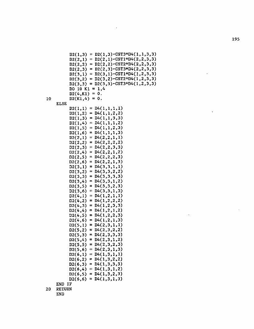
195
D 2 ( l , 3 ) = D 2 (1 ,3 ) -C S T 3 * D 4 (1 ,1 , 3 , 3 ) D 2 ( 2 ,1) = D 2 ( 2 ,1 ) -C S T 1 * D 4 (2 ,2 ,3 ,3 ) D 2 ( 2 ,2 ) = D 2 ( 2 ,2 ) - C S T 2 * D 4 ( 2 ,2 ,3 ,3 ) D 2 ( 2 ,3 ) = D 2 ( 2 ,3 ) - C S T 3 * D 4 ( 2 ,2 ,3 ,3 ) D 2 ( 3 ,1) = D 2 ( 3 ,1 ) - C S T 1 * D 4 ( 1 ,2 ,3 ,3 ) D 2 {3 ,2 ) = D 2 (3 ,2 ) -C S T 2 * D 4 (1 , 2 , 3 , 3 ) D 2 (3 ,3 ) = D2( 3 , 3 ) -CST3*D4(1 , 2 , 3 , 3 ) DO 10 Kl = 1 ,4 D2(4,K 1) = 0 .
10 D 2(K 1,4) = 0 .ELSE
D2( 1 1) = D4 1 1 1 1)D2( 1 2) = D4 1 1 2 2)D2( 1 3) = D4 1 1 3 3)D2( 1 4) = D4 1 1 1 2)D2( 1 5) = D4 1 1 2 3)D2( 1 6) = D4 1 1 1 3)D2(2 1) = D4 2 2 1 1)D2(2 2) = D4 2 2 2 2)D2(2 3) = D4 2 2 3 3)D2(2 4 ) = D4 2 2 1 2)D2(2 5) = D4 2 2 2 3)D2(2 6) = D4 2 2 1 3)D2(3 1) = D4 3 3 1 1)D2(3 2) = D4 3 3 2 2)D2(3 3) = D4 3 3 3 3)D2(3 4 ) = D4 3 3 1 2)D2(3 5) = D4 3 3 2 3)D2(3 6) = D4 3 3 1 3)D2(4 1) = D4 1 2 1 1)D2(4 2) = D4 1 2 2 2)D2(4 3) — D4 1 2 3 3)D2(4 4) = D4 1 2 1 2)D2(4 5) = D4 1 2 2 3)D2(4 6) = D4 1 2 1 3)D2(5 1) = D4 2 3 1 1)D2(5 2) — D4 2 3 2 2)D2(5 3) = D4 2 3 3 3)D2(5 4 ) = D4 2 3 1 2)D2(5 5) = D4 2 3 2 3)D2(5 6) = D4 2 3 1 3)D2(6 1) = D4 1 3 1 1)D2(6 2) = D4 1 3 2 2)D2(6 3) = D4 1 3 3 3)D2(6 4) D4 1 3 1 2)D2(6 5) = D4 1 3 2 3)D2(6 6) = D4 1 3 1 3)
END IF 20 RETURN
END

u u
u
APPENDIX D
CONTACT BOUNDARY SIMULATION MODULE
SUBROUTINE BOUNDCIDOF, NNDF, NINODE, ICODE, RFACT, IOUT)CC = = = = = = = = = = = = = = = = = = = = = = = = = = = = = = = = = = = = = = = = = = = = = = = = = = = = = = = = = = = = = = = = = = :
C IC l P R O G R A M :C IC I 'BOUND* CHECKS THE MOTION OF ROLLERS ON CURVEDC I BOUNDARIES AND INSURES THAT THE ROLLERS STAY ON THE BOUNDARYC l BY DETERMINING THE APPROPRIATE DISPLACEMENT CORRECTIONS.C IC l A R G U M E N T L I S T :C IC I IDOF(I)C I NNDFC I NINODEC I ICODEC I C IC I RFACTC I IOUTC IC =============C
IMPLICIT REAL*8 (A-H.O-Z)REAL*4 X,Y,ZCOMMON/MAIN1/U(8000),RE1(8000)C0MM0N/MAIN2/UT0TAL(8000)COMMON/MAIN4/RE(8000)COMMON/INPUT3/X(4000),Y(4000),Z(4000)COMMON/INPUT7/RIT(8O0O),RINC(8000),UINC(8000) COMMON/INPUTD/COSTX(300),COSTY(300),COSTZ(300) COMMON/INPUTE/ISPB(4000)COMMON/INPUTI/ INTFAC(5 0 0 )COMMON/CONTR1/INCREM, NIT DIMENSION IDOF( 1 )
CICODE = 0
- - - NINODE = NUMBER OF INTERFACE NODES
DO 100 Kl = 1 , NINODE IRLS = 0NODE = INTFAC( Kl )ID1 = NNDF*(NODE - 1) + 1 ID2 = ID1 + 1
= THE ARRAY CONTAINING THE D.O .F. NUMBERS = NUMBER OF NODAL DEGREES OF FREEDOM = NUMBER OF INTERFACE NODES = RETURN CODE PASSED TO THE CALLING ROUTINE
=0; NO CHANGE IN THE D.O .F. NUMBERS =1; RECALCULATION OF THE 'IDOF* ARRAY IS NEEDED
= REDUCTION FACTOR FOR OUTOMATIC SUBINCREMENTATION = OUTPUT DEVICE NUMBER
196

197
CC YNODE = FINAL Y-COORD OF THE NODEC
XNODE = X( NODE ) + UTOTALC ID1 )YNODE = Y( NODE ) + UTOTALC ID2 )
CC ----- CHECK TO SEE IF THE NODE IS IN CONTACT WITH THE BOUNDARYCC ---- FIND THE POINT ON THE DIE FOR A NORMAL RETURN CORRECTION.C - - - THE DIE IS MODELED USING THE HERMITE PARAMETRIC CURVE.C — SUBROUTINE MULLER FINDS THE PARAMETER ' T ' .C
CALL MULLER(XNODE, YNODE, T , NCURVE, IRET, IOUT)IF ( IRET.GE.2) THEN
WRITE(IOUT , 1001)STOP
ELSE IF (IRET.EQ.l) THENCC ---- SUBROUTINE HERMXY FINDS THE 'X' AND 'Y' COORDINATES OF THEC - - - RETURN POINT ON THE DIE.C
CALL XYPRIM(T,XP,YP,NCURVE)CALL HERMXY(T, XFINAL, YFINAL, NCURVE)DX = XFINAL - XNODE DY = YFINAL - YNODE IF (IDOF( ID1 ) . LE.0 ) THEN
RDOT = -YP*RE( ID1 ) + XP*RE( ID2 )DOT = - 1 .
ELSERDOT = - 1 .DOT = -YP*DX + XP*DY
END IFIF (RDOT.GE.0 . 0 . OR.DOT.GE.0 . 0 ) THEN
CC - - - CHANGE THE NEGATIVE "ISPB" ADDRESSES TO POSITIVE SO THATC THEY ARE RECOGNIZED IN THE SOLUTION PROCESSC
R = DSQRT(DX**2 + DY**2)RP = DSQRT(XP**2 + YP**2)IF (ISPB( NODE ).LT.O) THEN
ISPB( NODE ) = - ISPB( NODE )ELSE IF(ISPB( NODE ).EQ.O) THEN
WRITE(IOUT , 1000) NODE STOP
END IFCC ----- FIND THE DIRECTION COSINES OF THE ROLLERS ON THE DIEC
COSTX(ISPB( NODE ) ) = -YP/RP COSTY(ISPB( NODE ) ) = XP/RP
IF (IDOF( ID1 ) .GT.O) THEN ICODE = 1

IDOF( ID1 ) = -1 IDOF( ID2 ) = 1
ELSEIDOF( ID1 ) = -1
END IFCC ----- IMPOSE THE APPROPRIATE DISPLACEMENT FOR THE NORMAL RETURNC CORRECTION DURING THE NEXT ITERATION.C
DOT = -YP*DX + XP*DY IF (DOT.GE.O) THEN
UINC( ID1 ) = R/RFACTELSE
UINC( ID1 ) = -R/RFACT END IF
ELSEIRLS = 1
END IF END IFIF ( IRET.EQ. 0 .OR.IRLS.EQ.1) THEN
CC - - - IF THE NODE EXITS THE DIE RELEASE IT AND SET ICODE = 1 TO C THE CALLING ROUTINE RECALCULATES THE "IDOF" ARRAYC
UINC( ID1 ) = 0 .IF(ISPB( NODE ) . GT.0 ) ISPB( NODE ) = -ISPB( NODE )IF(IDOF( ID1 ) .LE.O ) THEN
ICODE = 1 IDOFC ID1 ) = 1RINCC ID1 ) = -RE( ID1 ) /RFACTRINC( ID2 ) = -RE( ID2 ) /RFACT
ELSERINCC ID1 ) = 0 .RINCC ID2 ) = 0 .
END IFC RITC ID1 ) = 0 .C RITC ID2 ) = 0 .
END IF 100 CONTINUE
CRETURN
1000 FORMATCIX, ' » » » > PROGRAM STOPED IN ROUTINE "BOUND" DUE TO A1/1 9X, ' ZERO ISPB FOR INTERFACE NODE ’ ,1 4 )
1001 FORMATCIX,1 > » » » PROGRAM STOPED IN ROUTINE "BOUND" DUE TO ’ /1 9X,'EXISTANCE OF MULTIPLE CONTACT POINTS')END

no
on
n
a n
or
an
no
on
nc
jn
nn
oc
jo
on
oo
nn
nn
nn
nn
nn
nn
oc
ici
199
M U L L E R =============
SUBROUTINE MULLER( XD, YD, TF, NCRV, IRET, IOUT)
II P R O G R A M :II 'MULLER' PERFORMES THE FOLLOWING FUNCTIONS:II 1) IT USES ZONING TO DETERMINE THE BOUNDARY CURVE WHICH ISI CLOSEST TO THE INTERFACE NODE.II 2 ) IT USES THE MULLERS METHOD TO SOLVE A FIFTH ORDERI POLYNOMIAL WHICH DETERMINES PARAMETER "T" WHICH ISI USED TO DETERMINE THE CLOSEST POINT ON A CURVE TO THEI INTERFACE NODE.II A R G U M E N T L I S T :II XD X-COORDINATE OF THE INTERFACE NODEI YD Y-COORDINATE OF THE INTERFACE NODEI TF FINAL VALUE OF PARAMETER "T"I NCRV = NUMBER OF BOUNDARY CURVES TO BE CHECKEDI IRET = CONDITION CODE RETURNED TO THE CALLING ROUTINEI =0; NO VALUE FOR "T" IF FOUND, NODE IS FREEI =1; A NORMAL FROM THE NODE TO ONE OF THE CURVESI MAY BE DRAWN INDICATING POSSIBILITY OF CONTACTI >1; TOO MANY NORMALS DETECTED, POSSIBLE ERRORII RFACT = REDUCTION FACTOR FOR OUTOMATIC SUBINCREMENTATIONI IOUT = OUTPUT DEVICE NUMBERI
- - - IRET = 0; NO CONTACT WITH BOUNDARIES
IMPLICIT REAL*8 (A-H.O-Z)COMMON/BOUND1/NCURVSCOMMON/ BOUND2/XZL( 6 ) ,X Z R (6),Y ZB (6),Y Z T(6)COMMON/ HERM/ H(4 , 4 ) ,GX(4 , 6 ) ,G Y (4 , 6 ) COM M ON/CONST/COC6),C1(6),C2(6),C3(6),C4(6),C5(6) DIMENSION ROOT(5)
TOL = .000000001 IRET = 0
IRET = 0; NO CONTACT WITH BOUNDARIES1; ONE CONTACT POINT DETECTED
<1; TOO MANY CONTACT POINTS (PROBABLE ERROR)
DO 60 NCURVE = 1 , NCURVSIF (XD. GT. XZR(NCURVE) . OR. XD. LT. XZL(NCURVE)) THEN

200
GO TO 60ELSE IF(YD.GT.YZT(NCURVE).OR.YD.LT.YZB(NCURVE) ) THEN
GO TO 60 END IF
CD5 = C5( NCURVE )D4 = C4( NCURVE )D3 = C3( NCURVE )D2 = C2( NCURVE ) + 3.*(XD*GX(1 , NCURVE) + YD*GY(1 , NCURVE))D1 = CI( NCURVE ) + 2.*(XD*GX(2 , NCURVE) + YD*GY(2 , NCURVE))DO = C0( NCURVE ) + XD*GX(3 , NCURVE) + YD*GY(3 , NCURVE)
CNROOT = 0
10 T1 = 0 .T2 = 1.TO = 0 .5
CFI = DOF2 = D5 + D4 + D3 + D2 + D1 + DO
CDO 20 Kl = 1 , NROOT FI = Fl/(-ROOT( Kl ) )F2 = F2/C1. - ROOT( Kl ) )
20 CONTINUEC
DO 40 Kl = 1 , 20FO = ((((D 5*T 0 + D4)*T0 + D3)*T0 + D2)*T0 + D1)*T0 + DO
CDO 30 K2 = 1 , NROOT
30 FO = FO/(TO - ROOT( K2 ) )C
H2 = TO - T2 HI = T1 - TO HIS = HI**2 GAM = H2/H1A = (GAM*F1 - F 0 * (1 .+GAM) + F2)/(GAH*H1S*(1 + GAM))B = (FI - FO - A*H1S)/H1
CSQTRM = B**2 - 4.*A*F0 IF (SQTRM.LT.O.) GO TO 60 IF (B .LE.O .) THEN
D = -DSQRT( SQTRM )ELSE
D = DSQRT( SQTRM )END IF
CT = TO - 2 .*F0/(B +D )
CIF (DABS(T-TO).LE.TOL) GO TO 50
CIF (T.GT.T0.AND.T.NE.T2) THEN
T1 = TO

201
TO = T FI = FO
ELSE IF(T.LT.TO.AND.T.NE.Tl) THEN T2 = TO TO = T F2 = FO
ELSEGO TO 50
END IF AO CONTINUE
C50 IF (T .G T .l . .O R .T .L T .O .) THEN
IF (NROOT.LT.4 ) THEN NROOT = NROOT + 1 ROOT( NROOT ) = T GO TO 10
END IFELSE
IRET = IRET + 1 TF = TNCRV = NCURVE RETURN
END IF 60 CONTINUE
CRETURNEND

o u
u
202
SUBROUTINE COEFIC IMPLICIT REAL*8 (A-H.O-Z)COMMON/BOUND1/NCURVSC0MM0N/HERM/H(4 , 4 ) ,G X (4 , 6 ) ,G Y (4 , 6) COMMON/CONST/CO(6 ) ,C 1 ( 6 ) ,C 2 ( 6 ) ,C 3 ( 6 ) ,C 4 ( 6 ) ,C 5 ( 6 )
CDO 10 Kl ~ 1 , NCURVS
C0( Kl ) = 0 .C l( Kl ) = 0 .C2( Kl ) =r 0.C3( Kl ) = 0.C4( Kl ) = 0 .C5( Kl ) s 0 .
C0( Kl ) 3 C0( Kl ) - GX(3 , K1)*GX(4 , K l)- GY(3 , K1)*GY(4 , K l)
C1( Kl ) = C1( Kl ) - GX(3 , K l)* * 2 - 2.*GX(2 , K1)*GX(4 , K l)- GY(3 , K l)* * 2 - 2.*GY(2 , K1)*GY(4 , K l)
C2( Kl ) = C2( Kl ) -3 .*G X (1,K 1)*G X (4,K 1)-3 .*G X (2,K 1)*G X (3,K 1)-3 .*G Y (1,K 1)*G YC4,K1)-3.*GY(2,K 1)*G Y(3,K 1)
C3( Kl ) C3( Kl ) - 2.*GX(2 , K l)* * 2 - 4.*GX(1 , K1)*GX(3 , K l)- 2 . *GY(2 , K l)* * 2 - 4.*GY(1 , K1)*GY(3 , K l)
C4( Kl ) = C4( Kl ) - 5 .*GX(1 , K1)*GX(2 , K l)- 5 . *GY(1 , K1)*GY(2 , K l)
C5( Kl ) = C5( Kl ) - 3 .*G X (1 , K l)* * 21 - 3 .*G Y (1 , K l)**2
10 CONTINUEC
RETURNEND

o o
o203
SUBROUTINE HERMIT IMPLICIT REAL*8 (A-H.O-Z)REAL*8 LX.LY C0MM0N/B0UND1/NCURVS C0MM0N/P0INTS/LX(4 , 6 ) ,LY(4 , 6)C0MM0N/HERM/H(4 , 4 ) ,G X (4 , 6 ) ,G Y (4 , 6 )
CDO 20 K2 = 1 , NCURVS DO 20 Kl = 1 , 4 GX(K1 , K2) = 0 .GY(K1 , K2) = 0.DO 20 K3 = 1 , 4GXCK1 , K2) = GX(K1 , K2) + H(K1 , K3)*LX(K3 , K2)
20 GYCK1 , K2) = GY(K1 , K2) + H(K1 , K3)*LY(K3 , K2)C
RETURNEND

u u
u
SUBROUTINE HERMXY(T,X,Y,NCURVE)IMPLICIT REAL*8 (A-H.O-Z)REAL*8 MC0MM0N/HERM/H(4 , 4 ) ,G X (4 , 6 ) ,G Y (4 , 6 ) DIMENSION M(4)
CM( 4 ) = 1.M( 3 ) = TM( 2 ) = T*M( 3 )M( 1 ) = T*M( 2 )
CX = 0 .Y = 0 .DO 20 Kl = 1 , 4X = X + M( Kl ) * GX(K1 , NCURVE)
20 Y = Y + M( Kl ) * GY(K1 , NCURVE)C
RETURNEND

n n
o205
SUBROUTINE XYPRIM( T, XP, YP, NCURVE) IMPLICIT REAL*8 (A -H ,0-Z)REAL*8 MPRIMC0MM0N/HERM/H(4 , 4 ) ,G X (4 , 6) ,G Y (4 , 6) DIMENSION MPRIM(4)
CMPRIM( 4 ) = 0 .MPRIM( 3 ) = 1.MPRIMC 2 ) = 2.*T MPRIM( 1 ) = 3.*T**2
CXP = 0.YP = 0.DO 20 Kl = 1 , 4XP = XP + MPRIM( Kl ) * GX(K1 , NCURVE)
20 YP = YP + MPRIM( Kl ) * GY(K1 , NCURVE)C
RETURNEND

nn
n
APPENDIX E
ELASTICITY MODULE
SUBROUTINE ELAST(ITYPE,MATNUM, IFLAG, IOUT, ICODE)C
IF ( ICODE.EQ.O) THENCALL DELAST(ITYPE,MATNUM,IFLAG)
ELSECALL STRSTNCITYPE, MATNUM, IFLAG, IOUT)
END IF RETURN END
==================== S T R S T N ==============================
SUBROUTINE STRSTN(ITYPE.MATNUM,IFLAG, IOUT)IMPLICIT REAL*8 (A -H ,0 -Z )CHARACTER*105 DUMMYC0MM0N/UTIL1/STRESS(6),STRAIN(6), DUMMY COMMON/MATER1/DEP(6 , 6 )COMMON/ELSTR1/STRN(6)C0MM0N/ELSTR2/STRS(6)COMMON/DEVICE/LDEV1 , LDEV2, LDEV3, LDEV4, LDEV5, LDKEEP, LDEV, LDEVST COMMON/CONTR1 / INCREM, NIT DIMENSION D E (6 ) ,D S (6 )
CIF ( ITYPE.GT.300) THEN
IEND = 6ELSE
IEND = 4 END IF
CIF ( INCREM.GT.l) THEN
CALL I0GET(LDEV1,96,' ( A 9 6 ) 1,5 )ELSE
DO 50 Kl = 1 , IEND STRESS( Kl ) = 0 .
50 STRAIN( Kl ) = 0 .END IF
CDO 100 Kl = 1 , IEND
100 DE( Kl ) = STRN( Kl ) - STRAIN( Kl )C
CALL DELASTfITYPE,MATNUM,IFLAG)C
DO 300 Kl= 1 , IEND S = 0 .DO 200 K2 = 1 , IEND
200 S = S + DEP(K1 , K2)*DE( K2 )
206

207
300 DS( Kl ) = SC
DO 400 Kl = 1 , IEND STRAINC Kl ) = STRN( Kl )STRESSC Kl ) = STRESS( Kl ) + DS( Kl )
400 STRSC Kl ) = STRESSC Kl )C
call ioputcldev2 , 9 6 , ' ca9 6 ) , ,5 )c
RETURN 1000 FORMATC2A48)
END

2 0 8
CC ====================== D E L A S T ============================C
SUBROUTINE DELAST(ITYPE, MATNUM, IFLAG)CC ===============================================================C IC I PROGRAM 'ELAST'EVALUATES THE STRESS-STRAIN STIFFNESS MATRIXC I FOR ISOTROPIC OR ORTHOTROPIC ELASTIC MATERIALSC IC l C O M M O N B L O C K SC I C IC ================================================================C
IMPLICIT REAL*8 (A -H ,0 -Z )REAL*8 NUX,NUY,NUZ COMMON/MATERl/DEP(6,6)COMMON/INPUT5/NUX(1 0 ) ,NUY(1 0 ) ,NUZ(1 0 ) ,E X (1 0 ) ,E Y (1 0 ) ,E Z ( 1 0 ) ,
1 P1X (1 0 ) ,P 1 Y (1 0 ) ,P 1 Z (1 0 ) ,P 2 X (1 0 ) ,P 2 Y (1 0 ) ,P 2 Z (10)C
IF ( ITYPE.GT.300) THENC
DO 100 K2 = 1 , 6 DO 100 Kl = 1 , 6
100 DEP(K1 , K2) = 0 .C
G = 0.5*EX ( MATNUM ) / ( l . + NUX( MATNUM ) )CST1 = 2 .* G * (1 . - NUX( MATNUM ) ) / ( l . - 2.*NUX( MATNUM ) )CST2 = 2.*G*NUX( MATNUM ) / ( l . - 2.*NUX( MATNUM ) )
CDEP( 1 1) = CST1DEP(2 2) = CST1DEP(3 3) = CST1DEP(4 4) = GDEP(5 5) = GDEP(6 6) = GDEP( 1 2) = CST2DEP( 1 3) = CST2DEP(2 1) = CST2DEP(2 3) = CST2DEP(3 1) = CST2DEP(3 2) = CST2
ELSE
DO 200 K2 == 1 , 4DO 200 Kl = 1 , 4
200 DEP(K1 , K2) = 0.CC PLAIN STRESSC

oo
n209
IF ( IFLAG.EQ.l) THENDEP(1 , 1) = EX( MATNUM ) / ( l . - NUX( MATNUM )* * 2 )DEP(2 , 2) = DEP(1 , 1)DEP(3 , 3) = EX( MATNUM ) * 0 . 5 / ( l . + NUX( MATNUM ) )DEP(1 , 2) = NUX( MATNUM )*DEP(1 , 1)DEP(2 , 1) = DEP(1 , 2)
AXISYMMETRIC AND PLANE STRAIN
ELSECST1 = EX( MATNUM ) / ( l . + NUX( MATNUM)) / ( 1 . CST2 = CST1*NUX( MATNUM )
- 2 . *NUX(MATNUM))
DEP( 1 1) = CST1 - CST2DEP(2 2) = DEP(1 , 1)DEP(3 3) = EX( MATNUMDEP(4 4) = DEP(1 , 1)DEP( 1 2) = CST2DEP(2 1) = . CST2DEP( 1 4 ) = CST2DEP(4 1) CST2DEP(2 4) = CST2DEP(4 2) = CST2
) * 0 . 5 / ( 1 . + NUX( MATNUM ) )
END IF END IF
RETURNEND

no
n
APPENDIX F
ELEMENT LIBRARY MODULE
= = = = = = = = = = = = = = = = = = = = = G A U S S = = = = = = = = = = = = = = = = = = = = = = = = = = = = =
SUBROUTINE GAUSS(NIP,W.GCOORD)CC =================================================================:C IC I SUBPROGRAM GAUSS STORES THE COORDINATES XI AND ETA OF THEC I NUMERICAL INTEGRATION POINTS AND THEIR WEIGHTING FUNCTIONSC I FOR THE FOUR POINT AND THE NINE POINT INTEGRATION.C IC I NIP = NUMBER OF THE INTEGRATION POINTSC l W(I) = WEIGTH FUNCTIONC I GCOORD(I) = COORDINATES OF THE GAUSSIAN POINTSC I FROM THE NEGATIVE TO POSITIVEC IC I FIRST DEVELOPED: 08-26-1988C I LAST UPDATE: 08-26-1988C l BY: M. FOROOZESHC ==================================================================
REAL*8 W,GCOORD DIMENSION W(4),GC00RD(4)
CIF (N IP .E Q .l) THEN
W( 1 ) = 2.0D0 GCOORDC 1 ) = 0.0D0
CELSE IF (NIP.EQ.2) THEN
W( 1 ) = l.ODOW( 2 ) = 1.0D0GCOORDC 1 ) = -0 .5 7 7 3 5 0 2 6 9 189626D0 GCOORD( 2 ) = 0 .57735026918962600
CELSE IF (NIP.EQ.3) THEN
W( 1 ) = 5.0DO/9.0DO W( 2 ) = 8 .0D 0/9 .0D 0W( 3 ) = W( 1 )GCOORDC 1 ) = - 0 . 774596669241483D0 GCOORDC 2 ) = 0 .GCOORDC 3 ) = 0 . 774596669241483D0
CELSE IF CNIP.EQ.4) THEN
W( 1 ) = 0.347854845137454DO WC 2 ) = 0.652145154862546D0 WC 3 ) = W( 2 )WC 4 ) = WC 1 )
210

no
n211
GCOORDC 1 ) = -0.861136311594053DOGCOORDC 2 ) = -0.339981043584856DOGCOORDC 3 ) = + 0 .339981043584856D0GCOORDC 4 ) = + 0 .861136311594053D0
CELSE
GO TO 10C
END IF 10 RETURN
END
====================== I R O N S ============================
SUBROUTINE IR0NSCA1,B6 ,C8 ,B,C,NIP,INTCOD)CC ================================================================C IC I SUBPROGRAM IRONS STORES THE COORDINATES RETURNS THE COORD.C I AND THE WEIGHT FUNCTIONS FOR THE OPTIMUM INTEGRATIONC I POINTS INTRODUCED BY BRUCE M. IRONS.C IC I FOR THE DISCRIPTION OF VARIABLES REFER TO THE REFERENCEC I PUBLICATION.C IC I FIRST DEVELOPED: 10-08 -1988C I LAST UPDATE: 10-08-1988C l BY: M. FOROOZESH
IMPLICIT REAL*8 CA-H.O-Z)C
IF CINTCOD.EQ.150) THEN NIP = 15A1 = 1 .5 64444444444D0 B6 = 0.3555555555556D0 C8 = 0.5377777777778D0 B = 1.0D0 C = 0 . 674199862D0
ELSE IFCINTCOD.EQ.151) THEN NIP = 15A1 = 0 . 712137436D0 B6 = 0.686227234D0 C8 = 0.396312395D0 B = O.848418O11D0 C = 0.727662441D0
ELSE IF(INTCOD.EQ.140) THEN NIP = 14 A1 = 0.0D0 B6 = . 886426593D0 C8 = . 335180055D0 B = 0 . 795822426D0 C = 0.758786911D0

212
END IFC
RETURNEND

on
n
n n
nn
nn
n
n n
o n
o n
nn
nn
nn
nn
nn
nn
nn
o
n o
213
=================== I S H A P E
SUBROUTINE ISHAPE
I THIS PROGRAM EVALUATES THE SHAPE FUNCTIONS, THEIR DERIVATIVESI WITH RESPECT TO THE NATURAL COORDINATES, AND THE WEIGHTI FUNCTIONS AT EACH INTEGRATION POINT.II ENTRY POINTS:I ISH2DG (FOR 2D ELEMENTS)I ISH3DG (FOR 3D ELEMENTS)II FIRST DEVELOPED: 0 8 -2 7 -1 9 8 8I LAST MODIFIED: 0 8 -2 9 -1 9 8 8I BY: M. FOROOZESHI
IMPLICIT REAL*8 (A -H ,0-Z)COMMON/ ISHAP2/W(2 7 )C0MM0N/INPUT1/NIPXI,NIPETA,NIPSI,NIP,INTCOD DIMENSION F (2 0 ) ,F X I (2 0 ) ,F E T A (2 0 ) ,F S I (2 0 )DIMENSION W X I(4),W E T A (4),W SI(4),X I(4) ,E T A (4),SI(4)
EVALUATE THE SHAPE FUNCTIONS OF THE 2D ISOPARAMETRIC ELEMENTS
ENTRY ISH2DG(ITYPE,NNEL, IERROR)
GET THE NATURAL COORDINATES OF THE INTEGRATION POINTS
CALL GAUSS(NIPXI,WXI,XI)CALL GAUSS( NIPETA, WETA, ETA)NIP = NIPXI*NIPETA
NIP = TOTAL NUMBER OF THE INTEGRATION POINTS FOR THE ELEMENT IETA = ROW NUMBER OF THE GAUSSIAN POINT FROM THE BOTTOM IXI = COLUMN NUMBER OF THE GAUSSIAN POINT FROM LEFT
DO 10 IETA = 1 , NIPETA DO 10 IXI = 1 , NIPXI
J = (IETA - 1)*NIPXI + IXIW( J ) = WXI( IXI )*WETA( IETA )AXI = XI( IXI )AETA = ETA( IETA )CALL IS0P2D(AXI,AETA,F,FXI, FETA,ITYPE,IERROR)CALL ISHEXT(NNEL,J,F,FXI,FETA,FSI)
RETURN

214
CCC EVALUATE THE SHAPE FUNCTIONS OF THE 3D ISOPARAMETRIC ELEMENTSC
ENTRY ISH3DG( ITYPE,NNEL,IERROR)C
CALL GAUSS(NIPXI,WXI,XI)CALL GAUSS(NIPETA,WETA,ETA)CALL GAUSS(NIPSI,WSI,SI)NIP = NIPXI*NIPETA*NIPSI I = NIPXI*NIPETA
CDO 20 IS I = 1 , NIPSI DO 20 IETA = 1 , NIPETA DO 20 IXI = 1 , NIPXI
J = ( I S I - 1 ) * I + (IETA - 1)*NIPXI + IXI W( J ) = WXI( IXI )*WETA( IETA )*WSI( IS I )AXI = XI( IXI )AETA = ETA( IETA )ASI a S I ( ISI )CALL ISOP3D(AXI, AETA,ASI,F,FXI, FETA, F S I , ITYPE, IERROR)
20 CALL ISHEXT(NNEL,J,F,FXI,FETA,FSI)C
RETURNCCCC
ENTRY ISH3DI(ITYPE,NNEL,IERROR)C
CALL IR0NS(A1,B6,C8,B,C,NIP,INTCOD)AXI = B AETA = 0 .ASI = 0 .DO 40 J = 1 , 6
W( J ) = B6CALL IS0P3D( AXI, AETA, A S I , F , FX I, FETA, F S I , ITYPE, IERROR)CALL ISHEXT( NNEL, J , F , FX I, FETA, F S I )A = AETA AETA = -AXI AXI = -ASI ASI = -A
40 CONTINUEC
AXI = C AETA = C ASI = CDO 60 J = 7 , 1 4
W( J ) = C8CALL IS0P3D(AXI,AETA,ASI,F,FXI,FETA,FSI,ITYPE,IERROR)CALL ISHEXT(NNEL,J,F,FXI,FETA,FSI)AXI = -AXI

215
A = AETA AETA = -ASIIF (J .E Q .1 0 ) AETA = ASI ASI = A
60 CONTINUEC
IF (INTCOD.GE.150) THEN W( 15 ) = A1 AXI = 0 .AETA = 0 .ASI = 0 .CALL IS0P3D( AXI, AETA, A S I, F , FXI, FETA, F S I , ITYPE, IERROR) CALL ISHEXT(NNEL, 1 5 , F , FXI, FETA, FSI)
END IFC
RETURNEND

^PROCESS DIRECTIVEC'*VDIR:' )CC =========================== I s H E X T ====================CC
SUBROUTINE ISHEXT(NNEL,J,F, FXI,FETA,FSI)REAL*8 N,NXI,NETA,NSI, F ,F X I , FETA,FSICOMMON/ISHAP1/N(2 0 , 2 7 ) ,N X I(2 0 , 2 7 ) ,NETA(20, 2 7 ) ,N S I ( 2 0 ,2 7 ) DIMENSION F ( 2 0 ) ,F X I (2 0 ) ,F E T A ( 2 0 ) ,F S I (2 0 )
CC*VDIR: ASSUME C0UNT(8)
DO 70 NN = 1 , NNEL N(NN , J ) = F( NN )NXI(NN , J ) = FXI( NN )NETACNN , J ) = FETA( NN )NSICNN , J ) = FSI( NN )
70 CONTINUEC
RETURNEND

217
CC =========================== E L M L I B ===========================C
SUBROUTINE ELMLIBCC ==================================================================C IC I SUBPROGRAM ELMLIB CALCULATES THE SHAPE FUNCTIONS AND THEC I PARTIAL DRIVATIVES OF THE SHAPE FUNCTIONS WRT THE LOCALC I COORDINATES ' X I ' , 'ETA* AND ' S l \C IC l N (I) = SHAPE FUNCTIONS OF THE ELEMENTC l NXI(I) = PARTIAL DRIVATIVE OF 'N' WRT 'XI'C I NETA(I) = PARTIAL DRIVATIVE OF 'N' WRT 'ETA'C l N S I(I ) = PARTIAL DERIVATIVE OF 'N' WRT 'S I 'C I C IC I FIRST DEVELOPED: 0 8 -2 7 -1 9 8 8C I LAST MODIFIED: 08 -2 7 -1 9 8 8C l BY: M. FOROOZESHC IC ===================================================================
REAL*8 X I , ETA,SI,N,NXI,NETA,NSI,XI0,ETA0,SI0 DIMENSION N (20),N X I(20),N E T A (20),N SI(20)COMMON/ELLIB1/XII(20),ETAI(20),SII(20)
CCC
ENTRY IS0P2D( X I, ETA, N, NXI, NETA, ITYPE, IERROR)CC DRIVATIVE OF SHAPE FUNCTIONS FOR 2D ISOPARAMETRIC ELEMENTS.CC
N X I(l ) = - 0 . 2 5 * ( 1 . - ETA)NXI(2) = 0 .2 5 * ( 1 . - ETA)NXI(3) = 0 .2 5 * ( 1 .+ ETA)NXI(4) = - 0 . 2 5 * ( 1 .+ ETA)NETA(l) = - 0 . 2 5 * ( 1 . - XI)NETA(2) = - 0 .2 5 * ( 1 .+ XI)NETAC3) = 0 .2 5 * ( 1 .+ XI)NETA(4) = 0 . 2 5 * ( 1 . - XI)
CIF (ITYPE.EQ.219) THEN
CST = 9 . D0/32.DO C13 = 1 . DO/3.DO C23 = 2 . DO/3.DONXI( 5 ) = CST*(1. - ETA)*(9.*XI**2 - 2 .*X I - 3 . )NXI( 6 ) = CST*(1. - ET A )*(-9 .*X I**2 - 2 .*X I + 3 . )NXI( 7 ) = 0 . 5 * ( 1. - ETA**2)NXI( 8 ) = -X I*(1 + ETA)NXI( 9 ) = - 0 .5 * ( 1 . - ETA**2)NXI( 1 ) = NXI( 1 ) -0 .5*N X I( 9 )-C23*NXI( 5 )-C13*NXI( 6 )
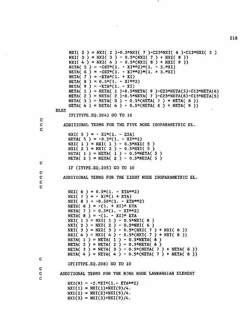
nr
sn
o
oo
oc
io
n
on
218
NXI( 2 ) = NXI( 2 ) -0 .5 * N X I ( 7 )-C23*NXI( 6 )-C13*NXI( 5 ) NXI( 3 ) = NXI( 3 ) - 0 .5 * (N X I( 7 ) + NXI( 8 ) )NXI( 4 ) = NXI( 4 ) - 0 .5 * (N X I( 8 ) + NXI( 9 ) )NETAC 5 ) = -C ST *(1 . - X I* * 2 )* C l . - 3 .* X I )NETA( 6 ) = -C ST *(1 . - X I* * 2 )* C l . + 3 .* X I )NETAC 7 ) = -ETA*C1 . + XI)NETA( 8 ) = 0 . 5 * ( 1 . - X I**2)NETAC 9 ) = -ETA *(1. - XI)NETA( 1 ) = NETA( 1 )-0.S*NETA( 9 )-C23*NETA(5)-C13*NETA(6)NETA( 2 ) = NETA( 2 )-0.5*N ETA ( 7 )-C23*NETA(6)-C13*NETA(5)NETA( 3 ) = NETAC 3 ) - 0.5*(NETA( 7 ) + NETA( 8 ) )NETAC 4 ) = NETA( 4 ) - 0.5*(NETA( 8 ) + NETA( 9 ) )
ELSEIF(ITYPE.EQ.2 0 4 ) GO TO 10
ADDITIONAL TERMS FOR THE FIVE NODE ISOPARAMETRIC EL.
NXI( 5 ) = - X I * ( 1 . - ETA)NETAC 5 ) = “0 . 5*C1• - X I**2)NXIC 1 ) = NXIC 1 ) - 0.5*NXIC 5 )NXIC 2 ) = NXIC 2 ) - 0.5*NXIC 5 )NETAC 1 ) = NETAC 1 ) - 0.5*NETAC 5 )NETAC 2 ) = NETAC 2 ) - 0.5*NETAC 5 )
IF CITYPE.EQ.2 0 5 ) GO TO 10
ADDITIONAL TERMS FOR THE EIGHT NODE ISOPARAMETRIC EL.
NXIC 6 ) = 0 .5 * C 1 . ” ETA**2)NXIC 7 ) = - XI*C1 + ETA)NXIC 8 ) = - 0 .50*C 1. - ETA**2 )NETAC 6 ) = - C l . + X I )* ETA NETAC 7 ) = 0 . 5*C1 . - XI**2 )NETAC 8 ) = - C l . - X I )* ETA NXIC 1 ) = NXIC 1 ) “ 0.5*NXIC 8 )NXIC 2 ) = NXIC 2 ) - 0.5*NXIC 6 )NXIC 3 ) = NXIC 3 ) - 0.5*CNXIC 7 ) + NXIC 6 ) )NXIC 4 ) = NXIC 4 ) - 0.5*CNXIC 7 ) + NXIC 8 ) ) NETAC 1 ) = NETAC 1 ) “ 0.5*NETAC 8 )NETAC 2 ) = NETAC 2 ) - 0.5*NETAC 6 )NETAC 3 ) = NETAC 3 ) - 0.5*CNETAC 7 ) + NETAC 6 ) ) NETAC 4 ) = NETAC 4 ) - 0.5*CNETAC 7 ) + NETAC 8 ) )
IFC ITYPE. EQ.2 0 8 ) GO TO 10
ADDITIONAL TERMS FOR THE NINE NODE LAGRANGIAN ELEMENT
NXIC9) = - 2 .*XI*C1 • - ETA**2) NXIC1) = NX ICl)+N XIC9)/4. NXIC2) = NXIC2)+NXIC9)/4. NXIC3) = NXIC 3 ) +NXIC 9 ) / 4 .

nn
o
a o
on
no
oo
219
NXI(4) = NXI( 4 ) +NXI( 9 ) / 4 . NXI(5) = N X I (5 ) -N X I (9 ) /2 .NXI( 6 ) = N X I (6 ) -N X I (9 ) /2 . NXI(7) = N X I(7 ) -N X I(9 ) /2 . NXIC8 ) = N X I (8 ) -N X I (9 ) /2 . NETA(9) = - 2 . * ETA*C1 . - XI**2) NETAC1) = NETACl)+NETA(9)/4. NETAC2) = NETA C 2 ) +NETA C 9 ) / 4 . NETAC3) = NETAC3)+NETAC9)/4. NETAC4) = NETAC4)+NETAC9)/4. NETAC5) = NETAC5 ) -NETAC9 ) / 2 • NETAC6 ) = NETAC6 ) -NETAC9 ) / 2 . NETAC7) = NETAC7 ) -NETAC9 ) / 2 . NETAC8) = NETAC8 ) -NETAC9)/2.
END IF
ENTRY N2DCXI,ETA,N,ITYPE,IERROR)
SHAPE FUNCTIONS FOR 2D ISOPARAMETRIC ELEMENTS.
10 NCI) = 0 .25*C1•“ XI)*C1.- ETA)NC2) = 0.25*C1.+ XI)*C1.- ETA)NC3) = 0.25*C1.+ XI)*C1.+ ETA)NC4) = 0.25*C1.“ XI)*C1-+ ETA)
IF CITYPE.EQ.219) THEN CST = 9 .DO/32.DO C13 = 1.DO/3.DO C23 = 2 .DO/3.DO
NCNCNCNC 8 ) =
NCNCNCNCNC
CST*Cl CST*C1 0.5*C1 0.5*C1 0.5*C1NCNC
) = NC ) = NC
ETA)*C1. - XI**2)*(1. ETA)*C1. - XI**2)*C1.
ETA**2)+ ETA) ETA**2)- C23*NC
3.*XI)3.*XI)
h XI)*C1. -- XI**2)*C1- XI)*Cl. - 0.5*NC 9 )0 .5*N C 7 ) 0.5*CNC 7 ) 0.5*CNC 8 )
5■ C23*NC 6 + NC 8 )) + NC 9 ))
C13*NCC13*NC
ELSEIFCITYPE.EQ.204) GO TO 15
ADDITIONAL TERMS FOR THE FIVE NODE ISOPARAMETRIC EL.
NC5) = 0.5*C1.- XI**2)*C1 .~ ETA)NCI) = NC1)-0.5*NC5)NC2) = N(2)-0.5*NC5)IF(ITYPE.EQ.205) GO TO 15
CC ADDITIONAL TERMS FOR THE EIGHT NODE ISOPARAMETRIC EL.

220
CN(6) = 0.5*(1.+ X I)*(1 .- ETA**2)N(7) = 0 .5*(1.- XI**2)*(1.+ ETA)N(8) = 0 .5* (1 .- XI)* ( ! • - ETA**2)N( 1) = N(1)-0.5*N(8)N (2) = N ( 2 ) -0 .5 * N (6 )N (3 ) = N (3 ) -0 .5 * (N (7 )+ N C 6 ))N (4 ) = N ( 4 ) - 0 .5 * ( N ( 7 ) + N ( 6 ) )
CIF(ITYPE.EQ.208) GO TO 15
CC ADDITIONAL TERMS FOR THE NINE NODE LAGRANGIAN ELEMENTC
N(9) = (1 .- ETA**2)*(1 .- XI**2)N (1) = N ( l ) + N ( 9 ) / 4 .N (2 ) = N (2 ) + N ( 9 ) /4 .NC3) = N (3 ) + N ( 9 ) /4 .N(4) = N(4)+N(9)/4.N(5) = N(5)-N(9)/2.N(6) = N(6)-N(9)/2.N(7) = N(7)-N(9)/2.N (8 ) = N ( 8 ) - N ( 9 ) / 2 .
END IFC
15 RETURNCCCC SHAPE FUNCTIONS AND THEIR DERIVATIVES FOR THE 3D ISOP. EL.C
ENTRY ISOP3D(XI,ETA,SI,N,NXI,NETA, NSI, ITYPE,IERROR)C
IF(ITYPE.EQ.308) THENC
DO 20 K = 1 , 8CALL ELMEXT(XI,ETA,SI,K,XIO,ETAO,SIO)N(K) = .125*(1. + XI0)*(1. + ETA0)*(1. + SIO)NXI(K) = . 125*(1. + ETA0)*(1. + SI0)*XII( K )NETA(K)= . 125*(1. + XI0)*(1. + SI0)*ETAI( K )NSI(K) = . 125*(1. + XI0)*(1. + ETA0)*SII( K )
20 CONTINUEC
ELSE IF ( ITYPE.EQ.320) THENCC HEXAHYDRON SOLID ELEMENTC SHAPE FUNCTIONS AND THIE DERIVATIVES FOR NODES 1-8.C
DO 30 K = 1 , 8CALL ELMEXT(XI,ETA,SI,K,XIO,ETAO,SIO)N(K) = . 125*(1. + XI0)*(1. + ETA0)*(1. + SI0)*(XI0+ETA0+ SIO-2.) NXI(K)=.125*(1. + ETA0)*(1. + SI0)*(2.*XI0+ETA0+ SI0-1.)*XII(K) NETA(K)=. 125*(1. + XI0)*(1. + SI0)*(XI0+2.*ETA0+ SI0-1. )*ETAI(K)

221
NSI(K)=.125*(1. + ETAO)*(1. + XI0)*(XI0+ETA0+2.*SI0-1.)*SII(K) 30 CONTINUE
CK1 = 9 K2 = 10
CC SHAPE FUNCTIONS AND THEIR DERIVATIVES FOR NODES 13-16.C
DO 40 K = 13 , 16CALL ELMEXT(XI,ETA,SI,K,XI0,ETA0,SI0)N(K) = .25*(1. + XI0)*(1. + ETA0)*(1. - SI**2)NXI(K)=.25*(1. + ETA0)*(1. - SI**2)*XII(K)NETA(K)=.25*(1. + XI0)*(1. - SI**2)*ETAI(K)NSI(K)=-0.5*(1. + ETA0)*(1. + XI0)*SI
CC SHAPE FUNCTIONS AND THEIR DERIVATIVES FOR NODES 9,11,17,19.C
CALL ELMEXT(XI,ETA,SI,K1,XI0,ETA0,SI0)N(K1) = . 25*(1. - XI**2)*(1. + ETA0)*(1. + SIO)NXI(K1)=-0.5*(1. + ETA0)*(1. + SI0)*XI NETA(K1)=.25*(1. - XI**2)*(1. + SI0)*ETAI(K1)NSI(K1)=.25*(1. + ETA0)*(1. - XI**2)*SII(K1)
CC SHAPE FUNCTIONS AND THEIR DERIVATIVES FOR NODES 10,12,18,20.C
CALL ELMEXT(XI,ETA,SI,K2,XI0,ETA0,SI0)N(K2) = .25*(1. + XI0)*(1. - ETA**2)*(1. + SIO)NXI(K2)=.25*(1. - ETA**2)*(1. + SI0)*XII(K2)NETA(K2)=-0.5*(1. + XI0)*(1. + SI0)*ETA NSI(K2)=.25*(1. - ETA**2)*(1. + XI0)*SII(K2)IF (K l.EQ .ll) THEN
K1 = 17 K2 = 18
ELSEK1 = K1 + 2 K2 = K2 + 2
END IF 40 CONTINUE
CEND IF
CRETURNEND

CJCJU u
uu
uu
oo
ou
o
u
222
E L M E X T
SUBROUTINE ELMEXT(XI, ETA, S I , K, XIO, ETAO, S I 0)
REAL*8 XI,ETA,SI,XIO,ETAO,SIO COMMON/ELLIB1/XII(20),ETAI(20),SII(20)
XIO = XI*XII( K )ETAO = ETA*ETAI( K ) SIO = SI*SII( K )
IIIII
FIRST DEVELOPED: 08-29-1988 LAST MODIFIED: 08-29-1988 BY: M. FOROOZESH
CRETURNEND

u u
u
223
@PROCESS DIRECTIVE('*VDIR:')
J A C O B I
CA
SUBROUTINE JACOBI
Ccc
II THIS
IPROGRAM CALCULATES THE JACOBIAN OF THE I
c I TRANSFORMATION BETWEEN THE LOCAL COORDINATES Ic I XI AND ETA AND THE GLOBAL COORDINATES X AND Y Icr
IT
FOR INTEGRATION POINT ’INTGPN' OF ELEMENT NUMBER 'NREL1. I
cX
I INTGPN =J.
INTEGRATION POINT NUMBER Ic I NREL ELEMENT NUMBER Ic I DETJAC = DETERMINANT OF THE JACOBIAN Ic I NX(I ) = PARTIAL DERIVATIVE OF N(I) WITH RESPECT TO X Ic I NY(I) = PARTIAL DERIVATIVE OF N(I) WITH RESPECT TO Y Ic I NZ(I) = PARTIAL DERIVATIVE OF N(I) WITH RESPECT TO Z Ic I IERROR = ERROR CODE FOR EXCESIVE ELEMENT DISTORTION Ic I =1 NO ERROR Ic I =-1 EXCESIVE ELEMENT DISTORTION(DETJAC<0) Icn
IT
NNEL NUMBER OF NODES(SHAPE FUNCTIONS) PER ELEMENT ITKj
c1
I NXI(I) =1
PARTIAL DERIVATIVE OF N(I) WITH RESPECT TO XI Ic I NETA(I) = PARTIAL DERIVATIVE OF N(I) WITH RESPECT TO ETA Ic I NSI(I) = PARTIAL DERIVATIVE OF N(I) WITH RESPECT TO SI Ic I X(IK) = NODE COORDINATE X, IK=GLOBAL NODE NUMBER, Ic I Y(IK) = NODE COORDINATE Y, IK=GLOBAL NODE NUMBER, Ic I Z(IK) = NODE COORDINATE Z, IK=GLOBAL NODE NUMBER, Ic I XXI PARTIAL DERIVATIVE OF X WITH RESPECT TO XI Ic I XETA PARTIAL DERIVATIVE OF X WITH RESPECT TO ETA Ic I XSI PARTIAL DERIVATIVE OF X WITH RESPECT TO SI Ic I YXI PARTIAL DERIVATIVE OF Y WITH RESPECT TO XI Ic I YETA PARTIAL DERIVATIVE OF Y WITH RESPECT TO ETA Ic I YSI PARTIAL DERIVATIVE OF Y WITH RESPECT TO SI Ic I ZXI PARTIAL DERIVATIVE OF Z WITH RESPECT TO XI Ic I ZETA PARTIAL DERIVATIVE OF Z WITH RESPECT TO ETA Icc
II
ZSI PARTIAL DERIVATIVE OF Z WITH RESPECT TO SI II
cc
II FIRST
IDEVELOPED: 08-27-1988 I
c I LAST MODIFIED: 08-27-1988 Ic I
TBY: M. FOROOZESH I
T
p 1 1
cIMPLICIT REAL*8 (A-H,0-Z)REAL*8 N,NXI,NETA,NSI,NX,NY,NZ REAL*4 X,Y,ZC0MM0N/ISHAP1/N(20,27),NXI(20,27 ),NETA(20,27),NSI(20,27) COMMON/INPUT2/NOP(20,2000)

COMM0N/INPUT3/X(40O0),Y(4000),Z(4000) COMMON/JACOBl/NX(2O),NY(20),NZ(20)
CCCCCC
ENTRY JACB2D(INTGPN, NREL, NNEL, IERROR, DETJAC)C
XXI = 0 .0 XETA = 0 . 0 YXI = 0 . 0 YETA = 0 . 0
CC*VDIR: ASSUME COUNT(8)
DO 10 K1 = 1 , NNEL NODE = N0P(K1 , NREL)XXI = XXI + NXI(K1,INTGPN)*X( NODE )XETA = XETA + NETA(K1, INTGPN)*X( NODE )YXI = YXI + NXI(K1,INTGPN)*Y( NODE )YETA = YETA + NETA(K1, INTGPN)*Y( NODE )
10 CONTINUEC
DETJAC = XXI*YETA - YXI*XETACC*VDIR: ASSUME COUNT(8)
DO 20 K = 1 , NNELNX(K) = (YETA*NXI(K,INTGPN) - YXI*NETA(K, INTGPN)) /DETJAC NY(K) = ( -XETA*NXI(K,INTGPN) + XXI*NETA(K,INTGPN)) /DETJAC
20 CONTINUE RETURN
CCCCCC
ENTRY JACB3DCINTGPN, NREL, NNEL,IERROR.DETJAC)C
XXI = 0 . 0 XETA = 0 . 0 XSI = 0 . 0 YXI = 0 . 0 YETA = 0 . 0 YSI = 0 .0 ZXI = 0 .0 ZETA = 0 . 0 ZSI = 0 . 0
CC*VDIR: ASSUME C0UNT(20)
DO 30 K1=1,NNEL

225
NODE = NOP(Kl , NREL)XXI = XXI + NXI(K1,INTGPN)*X( NODE )XETA = XETA + NETA(K1,INTGPN)*X( NODE )XSI = XSI + NSI(K1,INTGPN)*X( NODE )YXI = YXI + NXI(K1,INTGPN)*Y( NODE )YETA = YETA + NETA(K1, INTGPN)*Y( NODE )YSI = YSI + NSI(K1,INTGPN)*Y( NODE )ZXI = ZXI + NXI(K1, INTGPN)*Z( NODE )ZETA = ZETA + NETACK1,INTGPN)*Z( NODE )ZSI = ZSI + NSI(Kl,INTGPN)*Z( NODE )
30 CONTINUEC
DETJAC= XXI*(YETA*ZSI - ZETA*YSI) - YXI*(XETA*ZSI - ZETA*XSI) + 1 ZXI*(XETA*YSI - YETA*XSI)
CC*VDIR: ASSUME COUNT(20)
DO 40 K = 1 , NNELNX(K) = ((YETA*ZSI - ZETA*YSI)*NXI(K,INTGPN)
1 -(YXI*ZSI - ZXI*YSI)*NETA(K,INTGPN)2 +(YXI*ZETA - ZXI*YETA)*NSI(K,INTGPN))/DETJACNY(K) = (-(XETA*ZSI - ZETA*XSI)*NXI(K,INTGPN)
1 +(XXI*ZSI - ZXI*XSI)*NETA(K,INTGPN)2 -(XXI*ZETA - ZXI*XETA)*NSI(K, INTGPN)) /DETJACNZ(K) = ( (XETA*YSI - YETA*XSI)*NXI(K,INTGPN)
1 -(XXI*YSI - YXI*XSI)*NETA(K,INTGPN)2 +(XXI*YETA - YXI*XETA)*NSI(K,INTGPN))/DETJAC
40 CONTINUEC
RETURNEND

C3 O
CS226
:======================= E L I N F 0 ==================
SUBROUTINE ELINFO(ELNUM, ITYPE, NNEL, IFLAG, ISTART,LINES)ccc Ic I P R 0 G R A M Ic Ic I PROGRAM 'ELINFO' EXTRACTS ELEMENT INFORMATION FROM THE ARRAY Ic I 1INFOEL'.c Ic I A R G U M E N T L I S T Ic Ic I ELNUM ELEMENT NUMBER PASSED BY THE CALLING ROUTINE Ic Ic I ITYPE ELEMENT TYPE PASSED TO THE CALLING ROUTINE Ic Ic I NNEL NUMBER OF NODES IN THE ELEMNT PASSED TO THE Ic I CALLING ROUTINE Ic Ic I MATNUM MATERIAL I.D . NUMBER FOR THE ELEMENT PASSED TO THE Ic I CALLING ROUTINE Ic Ic I ISTART STARTING POSITION OF THE LINE CONNECTIVITY DATA Ic I IN ARRAYS 'IS ' AND 'I E 1. Ic Ic I LINES NUMBER OF LINES CONNECTING THE NODES WITHIN THE Ic I ELEMENT Icc
I
INTEGER ELNUM REAL*8 THICKCOMMON/INPUTA/INFOEL(2,2000),ETHICK(2000)
CI = INFOELQ , ELNUM)I I = INF0ELC2 , ELNUM)LINES = IANDCI1 , 8 2 5 7 5 3 6 ) /1 3 1 0 7 2 ISTART = 11 /83 8 8 6 0 8IFLAG = IAND(I , 1835008 )/2 6 2 1 4 4ITYPE = IAND(I , 2 6 1632 ) / 5 12NNEL = IAND(I , 5 0 8 ) / 8
CRETURN
CENTRY ELINTM(ELNUM,IDENT,INTCOD,NIPXI,NIPETA,NIPSI, MATNUM,THICK)I * INFOELf1 , ELNUM)I I = INF0ELC2 , ELNUM)MATNUM = IAND(I , 7 )NIPSI = 1 /134217728NIPETA = IAND(I , 117440512)/16777216 NIPXI = IAND(I , 14680064)/2 0 9 7 152

INTCOD = IAND(I1 , 255)IDENT = IAND(II , 1 3 0 8 16 ) /256 THICK = ETHICKC ELNUM )RETURNEND

o o
o
APPENDIX G
I/O MODULE
======================= C 0 M P R 0 ===========================
SUBROUTINE COMPROC BUFFER, BUFF, COMM, NEXT, K)INTEGER SPACE, COMMA, ZERO, NINE, DOT CHARACTER*80 BUFFER, BUFF, BUFER1 , BUFFI CHARACTER*1 LINE(80),C0M(4),COMLIN(80)CHARACTER*4 COMM,COMM1EQUIVALENCE ( BUFER1 , LINE) , ( COM, COMM1 ) , ( BUFF1 , COMLIN)DATA SPACE, COMMA, ZERO, NINE, DOT, MINUS/64, 1 0 7 , 2 4 0 , 2 4 9 , 7 5 , 9 6 /
BUFER1 = BUFFER
IFL = 0 BUFFI = * 'NEXT = 0 K1 = 0
110 K = K + 1 K1 = K1 + 1NCHAR = ICHAR(LINE( K ) )IF (K.EQ.80) THEN
GO TO 120ELSE IF (NCHAR.GE.ZERO.AND.NCHAR.LE.NINE) THEN
IFL = 1ELSE IF ( IFL.EQ.l.AND.NCHAR.NE.SPACE.AND.NCHAR.NE.DOT) THEN
NEXT = 1 K = K - 1 K1 = K1 - 1 GO TO 120
END IFCOMLINC K1 ) = LINE( K )GO TO 110
C120 IFL = 0
COMM1 = ’ 'ICOUNT = 0DO 130 K2 = 1 , K1NCHAR = ICHAR(COMLINC K2 ) )IF (NCHAR.EQ.SPACE.OR.NCHAR.EQ.DOT.OR.NCHAR.EQ.MINUS) THEN
GO TO 130ELSE IF (NCHAR.LT.ZERO.OR.NCHAR.GT.NINE) THEN
ICOUNT = ICOUNT + 1IF (ICOUNT.LE.4 ) COM( ICOUNT ) = COMLINC K2 )COMLINC K2 ) = ’ 1
END IF 130 CONTINUE
228

BUFF = BUFFI BUFFER = BUFER1 COMM = COMM1 RETURN END

non
n
nn
nn
n
nn
no
nn
na
n
nn
o230
==================== I N P U T ===
SUBROUTINE INPUT(IDOF,IOUT,IERROR)
II SUBROUTINE INPUT2 READS ALL THE INPUT INFORMATION FROMI CARD SETS 2 THROUGH 10. IT ALSO READS THE INFORMATION FROMI THE PRIVIOUS RUNS IF THE PROGRAM IS RESUBMITED.III
IMPLICIT REAL*8 (A-H.O-Z)REAL*8 NUX, NUY, NUZ, LX, LY REAL*4 X, Y, Z, FMAG, DMAG, ETHICK tTHICK CHARACTER*80 BUFFER, BUFF,TITEL CHARACTERS COMM COMMON/MAIN1/U(8000),RE1(8000)COMMON/INPUT2/NOP(2 0 ,2 0 0 0 )COMMON/INPUT3/X(4000),Y(4000),Z(4000)COMMON/INPUT5/NUXC1 0 ) ,NUY(1 0 ) ,NUZ(1 0 ) ,EX(1 0 ) ,E Y (1 0 ) ,E Z (1 0 ) ,
1 P 1 X (1 0 ) ,P 1 Y ( 1 0 ) ,P 1 Z ( 1 0 ) ,P 2 X ( 1 0 ) ,P2Y (1 0 ) ,P 2 Z (10)COMMON/INPUT6/WGTX(1 0 ) ,WGTY(10),WGTZ(10)COMMON/INPUT7/RX(8 0 0 0 ) ,R Y (8000),R Z (8000)COMMON/INPUT8/NNODES, N.ELEM, NNDF, NLINC, MNIT, IFLAG1, IFLAG2, IDIM,
1 NINODECOMMON/INPUTA/INFOEL(2 , 2 0 0 0 ) ,ETHICK(2000)COMMON/INPUTB/FAC, FACNEW, FACLOW, FACHIG, ENRG1 , NDIVER, ISTOP COMMON/INPUTC/TITELCOMMON/INPUTD/COSTX(300),COSTY(300),COSTZ(300)COMMON/INPUTE/ISPB(4000)COMMON/INPUTF/MATYPE(10)COMMON/INPUTG/IFLAG3, IOINTR, IFPLOT COMMON/BOUND1/NCURVSCOMMON/BOUND2/XZL(6),XZR(6),YZB(6),YZT(6)COMMON/INPUTI/INTFAC(500)C0MM0N/P0INTS/LX(4 , 6 ) , LY(4 , 6 )DIMENSION IDOFC1 ) ,DUMMY(6),M(20)
ICNT = COUTER FOR THE 'ISPB* ARRAY WHICH DETERMINES WHERE TO LOOK FOR THE DIRECTION COSINES OF THE SKEW BOUNDARY IN THE 'COSTX1, 'COSTY' AND 'COSTZ* ARRAYS.
ICNT = 1
READ THE COMMAND LINE BUFFER
LDEV11 = 11 100 IPOS = 0
READ(LDEV11 , 101 ,END=1000) BUFFER

n o
o o
o n
231
101 FORMAT(A80)C
105 CALL COMPROCBUFFER,BUFF,COMM,N,IPOS) IF(N.EO.O) THEN
ASSIGN 100 TO NEXTELSE
ASSIGN 105 TO NEXT END IF
EXTRACT THE FIRST FOUR CHARACTERS OF THE BUFFER AND REPLACE ALL OTHER CHARACERS BY A BLANK EXCEPT NUMBERS 1-9.
IF (COMM.EQ.'TITE') THEN GO TO 200
ELSE IF (COMM.EQ.'COOR*.OR.COMM.EQ.'NODE'.OR.COMM.EQ.'JOIN') THEN GO TO 300
ELSE IF (COMM.EQ.'MEMB*.OR.COMM.EQ.'INCI'.OR.COMM.EQ.'CONE') THEN GO TO 400
ELSE IF (COMM.EQ.'DISP') THENCALL IODISP(IDOF, NNDF, IDIM, ICNT, LDEV11 , IOUT)GO TO 100
ELSE IF (COMM.EQ.'LOAD') THEN CALL IOLOAD(LDEVll, IOUT)GO TO 100
ELSE IF (COMM.EQ.'GRAP') THENREAD(BUFF , * , END = 2000) IFPLOT CALL GRAPHX( LDEV1 1 , IOUT)GO TO 100
END IFIF (COMM.EQ.'MATE') THEN
READ(BUFF , * , END = 2000) MATNUM ELSE IF (COMM.EQ.'STOP') THEN
READ(BUFF , * , END=2000) ISTOP ELSE IF (COMM.EQ.'LINE') THEN
IFLAG1 = 0 ELSE IF (COMM.EQ.'NONL') THEN
IFLAG1 = 1 ELSE IF (COMM.EQ.'NONS') THEN
IFLAG2 = 1 ELSE IF (COMM.EQ.'SYMM') THEN
IFLAG2 = 0 ELSE IF (COMM.EQ.'ELEM') THEN
GO TO 440 ELSE IF (COMM.EQ.'DIME') THEN
READ(BUFF , * , END = 2000) IDIM NNDF = IDIM
ELSE IF (COMM.EQ.'ITER') THENREAD(BUFF , * , END = 2000 ) MNIT
ELSE IF (COMM.EQ.'INCR') THENREAD(BUFF , * , END = 2000) NLINC

232
ELSE IF (COMM.EQ.'FACL') THENREAD(BUFF , * , END = 2000 ) FACLOW FAC = FACLOW
ELSE IF (COMM.EQ.’FACH’ ) THENREAD(BUFF , * , END = 2000 ) FACHIG
ELSE IF (COMM.EQ.'NU') THENREAD(BUFF , * , END = 2000 ) NUX(MATNUM)
ELSE IF (COMM.EQ.'E') THENREAD(BUFF , * , END = 2000 ) EX(MATNUM)
ELSE IF (COMM.EQ.'WX') THENREAD(BUFF , * , END = 200 0 ) WGTX(MATNUM)
ELSE IF (COMM.EQ.'WY’ ) THENREAD(BUFF , * , END = 2000) WGTY(MATNUM)
ELSE IF (COMM.EQ.'WZ') THENREAD(BUFF , * , END = 2000) WGTZ(MATNUM)
ELSEGO TO 150
END IF GO TO NEXT
150 IF (COMM.EQ.'TYPE') THENREAD(BUFF , * , END = 2000) MATYPE( MATNUM )
ELSE IF(COMM.EQ.'YIEL') THENREAD(BUFF , * , END = 2000 ) P1Z( MATNUM )
ELSE IF(COMM.EQ.rISOT') THENREAD(BUFF , * , END = 2000) P1Y( MATNUM )
ELSE IF(COMM.EQ.'KINE1) THENREAD(BUFF , * , END = 2000) P1X( MATNUM )
ELSE IF(COMM.EQ.'REST') THEN IFLAG3 = 1
ELSE IF(COMM.EQ.'OUTP') THENREAD(BUFF , * , END = 2000 ) IOINTR
ELSE IF(COMM.EQ.'INTE') THEN GO TO 1100
ELSEGO TO 155
END IF GO TO NEXT
155 IF (COMM.EQ.'PAX') THENREAD(BUFF , * , END = 20 0 0 ) LX(1 , NCURVE)
ELSE IF(COMM.EQ.'PAY') THENREAD(BUFF , * , END = 20 0 0 ) LY(1 , NCURVE)
ELSE IF(COMM.EQ.'PBX') THENREAD(BUFF , * , END = 2000) LX(2 , NCURVE)
ELSE IF(COMM. EQ. ' PBY' ) THENREAD(BUFF , * , END = 2000) LY(2 , NCURVE)
ELSE IF(COMM.EQ.’RAX') THENREAD(BUFF , * , END = 200 0 ) LX(3 , NCURVE)
ELSE IF(COMM.EQ.'RAY') THENREAD(BUFF , * , END = 200 0 ) LY(3 , NCURVE)
ELSE IF(COMM.EQ.*RBX') THENREAD(BUFF , * , END = 2000 ) LX(4 , NCURVE)
ELSE IF(COMM.EQ.'RBY') THEN

o o
o u
uu
233
READ(BUFF , * , END = 2000) LY(4 , NCURVE)ELSE IF(COMM.EQ.'CURV') THEN
READ(BUFF , * , END = 2000) NCURVE IF (NCURVE.GT.NCURVS) NCURVS = NCURVE
ELSE IF(COMM.EQ.'XZL') THENREAD(BUFF , * , END = 2000) XZL(NCURVE)
ELSE IF(COMM.EQ. *XZR' ) THENREAD(BUFF , * , END = 2000) XZR(NCURVE)
ELSE IF(COMM.EQ.'YZB') THENREAD(BUFF , * , END = 2000) YZB(NCURVE)
ELSE IF(COMM.EQ.'YZT') THENREAD(BUFF , * , END = 2000) YZT(NCURVE)
ELSEGO TO 3000
END IF GO TO NEXT
READ THE TITEL OF THE PROGRAM (CARD SET1)
200 READ(BUFF , * , END = 2000) NUMBER DO 210 K = 1 , NUMBER READCLDEVll , 101) TITEL
210 WRITE( IOUT , 101) TITEL GO TO NEXT
READ AND GENERATE THE NODAL COORDINATES
300 1=0READ(BUFF , * , END = 2000) NNODES
310 READ (LDEV11 , * ) K,(DUMMY( IDIR ) , IDIR = 1 , IDIM),INCR C
X( K ) = DUMMY( 1 )Y( K ) = DUMMY( 2 )Z( K ) = DUMMY( 3 )
C1=1+1IF (INCR.EQ.O) GO TO 330N=(K-K1)/INCRDX=(X(K)-X(K1))/NDY=(Y(K)-Y(K1))/NDZ=(Z(K)-Z(K1))/NK2=K-INCRDO 320 J=K1,K2,INCR N1=(J-K1)/INCR X(J)=X(K1)+N1*DX Y(J)=Y(K1)+N1*DY Z(J)=Z(K1)+N1*DZ 1=1+1
320 CONTINUE 1=1-1
330 K1=KIF(I.LT.NNODES) GO TO 310

no
n2 34
WRITEflOUT , 6009)DO 340 K1 = 1 , NNODES
340 WRITEflOUT , 5 0 0 4 )K l ,X f K1 ) ,Y f K1 ) , Z ( K1 )GO TO NEXT
READ AND WRITE AND GENERATE THE ELEMENTS
400 I = 0READCBUFF , * , END = 2000) NELEM
410 READfLDEVll , *)K,ITYPE,NNEL,(NOP(NODE,K),NODE=l, NNEL), INCR ID = ITYPE/1000 ID1 = ITYPE - ID*1000 IFLAG = ID 1/100 ID2 = ID1 - IFLAG*100 ITYPE = ID*100 + ID2 IF ( ITYPE.LT.300) THEN
IF (NNEL.EQ.4) THEN ISTART = 1 LINES = 4
ELSE IFfNNEL.EQ.5) THEN ISTART = 5 LINES = 5
ELSE IF(ITYPE.EQ.2 0 8 . OR.ITYPE.EQ.2 0 9 ) THEN ISTART = 1 0 LINES = 8
ELSE IF(ITYPE.EQ.2 1 9 ) THEN ISTART = 5 4 LINES = 9
END IFELSE IF(ITYPE.GT.300) THEN
IF (NNEL.EQ.8) THEN ISTART = 1 8 LINES = 12
ELSE IF(NNEL.EQ.20) THEN ISTART = 30 LINES = 24
END IF END IF
1 = 1 + 1INF1 = NNEL*8 + ITYPE*512 + IFLAG*262144 INF2 = 8388608*ISTART + 131072*LINES INFOELf1 , K) = INFOELfl , K) + INF1 INFOEL(2 , K) = INFOEL(2 „ K) + INF2 IF(INCR.EQ.O) THEN
K1 = KELSE
K2 = (K - KD/INCR DO 420 NODE = 1 , NNEL
420 M( NODE ) = (NOPfNODE , K ) - NOPfNODE , K l) ) /K 2 C

DO 430 IELEM = Kl+INCR , K-INCR , INCR INFOEL(l , IELEM) = INFOELf1 , IELEM) + INF1 INF0EL(2 , IELEM) = INF0EL(2 , IELEM) + INF2 1 = 1 + 1IELEM1 = IELEM - INCR DO 430 NODE = 1 , NNEL
430 NOPfNODE , IELEM) = NOPfNODE , IELEM1) + Mf NODE )END IFIFfI.LT.NELEM) GO TO 410 GO TO NEXT
CC ........... READ AND GENERATE ELEMENT INFORMATIONSC
440 READfBUFF , * , END = 2000) ISTART IEND = ISTART INTR = 1 NIPXI = 0 NIPETA = 0 NIPSI = 0 INTCOD = 0 THICK = 0 .
450 CALL COMPROfBUFFER,BUFF,COMM,N,IPOS)IF fCOMM.EQ.'TO') THEN
READfBUFF , * , END = 2000) IEND ELSE IFfCOMM.EQ.'BY') THEN
READfBUFF , * , END = 2000) INTR ELSE IFfCOMM.EQ.'NIPX') THEN
READfBUFF , * , END = 2000) NIPXI ELSE IFfCOMM.EQ.'NIPE*) THEN
READfBUFF , * , END = 2000 ) NIPETA ELSE IFfCOMM.EQ.'NIPS’ ) THEN
READfBUFF , * , END = 2000) NIPSI ELSE IFfCOMM.EQ.'IRON') THEN
READfBUFF , * , END = 2000) INTCOD ELSE IF fCOMM.EQ.'THIC') THEN
READfBUFF , * , END = 2000) THICK ELSE IF fCOMM.EQ.'MATE') THEN
READfBUFF , * , END = 2000) MATELSE
GO TO 3000 END IFIF fN.NE.O) GO TO 450
CINF1. = 2097152*NIPXI + 16777216*NIPETA + 134217728+NIPSI + MAT INF2 = INTCOD + 256*fINTCOD + NIPXI + 10*NIPETA + 100*NIPSI)DO 460 K = ISTART , IEND , INTR ETHICKf K ) = ETHICKf K ) + THICK INFOELf1 , K) = INFOELf1 , K) + INF1
460 INFOELf2 , K) = INFOELf2 , K) + INF2 GO TO 100
CC ........... READ AND GENERATE THE INTERFACE NODES

236
1100 1 = 0READfBUFF , * , END = 2000) NINODE
1110 READ (LDEV11 , * ) K.INCR IF(INCR.EQ.O) THEN
1 = 1 + 1 INTFACf I ) = K IF (ISPB( K ) . EQ.0 ) THEN
ISPBf K ) = -ICNT ICNT = ICNT + 1
END IFELSE
ISTART = INTFACf I ) + INCR IEND = KDO 1130 J = ISTART , IEND , INCRIF (ISPBf J ) .EQ.O) THEN
ISPBf J ) = -ICNT ICNT = ICNT + 1
END IF 1 = 1 + 1
1130 INTFACf I ) = JEND IFIF (I.LT.NINODE) GO TO 1110 GO TO NEXT
C3000 WRITEflOUT , 3001)3001 FORMATfIX,'COMMAND ENTERED IS NOT RECOGNIZED BY *SAFE*' )2000 STOP1000 RETURN5004 FORMATf1 5 , IP , 3G20.1 0 )6002 FORMATf//.IX,'PHYSICAL DIMENSION = ' , 1 3 / IX,'NUMBER OF NODES = ' ,
1 1 6 / IX,'NUMBER OF ELEMENTS = ' ,I6/1X,'NUMBER OF NODAL D.O.F. = ' ,2 1 6 / ,3 IX,'NUMBER OF APPLIED NODAL LOADS = ' , 1 6 / IX,'NUMBER OF IMPOSED'4 , ' NODAL DISPLACEMENTS = ' , 1 6 / IX,'NUMBER OF SKEW BOUNDARIES = ' ,5 1 6 / IX,'INTEGRATION CODE = ' , I6/1X,'NUMBER OF LOAD INCREMENTS = '6 ,I6/1X,'GEOMETRIC LINEAR/NONLINEAR CODE = ’ , 1 6 / IX,'MAXIMUM ' ,7 'NUMBER OF ITERATION ALLOWED = ' , 1 6 / IX,'FACTOR = ' ,F 1 4 .7 )
6009 FORMATf/,20X,'COORDINATES OF THE NODES'/' NODE NO.' , 1 1 X , 'X ' ,# 1 9 X , 'Y ' ,1 9 X , 'Z ' / )
END

on
n237
I 0 D I S P =================
SUBROUTINE IODISP(IDOF, NNDF, IDIM, ICNT,LDEV1 1 , IOUT) IMPLICIT REAL*8 (A -H ,0-Z)CHARACTER*80 BUFFER,BUFF CHARACTERS COMM COMMON/MAINl/U(8O0O),RE1(8000)COMMON/INPUTD/C0STX(3 0 0 ) ,COSTY(300),COSTZ(300) COMMON/INPUTE/ISPBC4000)DIMENSION ID O F (l) ,D (3),ID 0(3),T H E T A (3)
ITIME = 0CST = 3 . 141592653589793DO/180.DO IF (IDIM.EQ.2) THEN
CST1 = 90.ELSE
CST1 = 0 .END IF
C10 IPOS = 0
READ(LDEV11 , ' (A 8 0 )' , END = 1000) BUFFER 20 CALL COMPRO(BUFFER,BUFF,COMM,N,IPOS)
CIF (COMM.EQ.'NODE') THEN
IF(ITIME.EQ.l) THENASSIGN 30 TO NEXT GO TO 60
END IF30 READ(BUFF , * , END=3000) ISTART
ITIME = 1 ISP = 0 IEND = ISTART INTR = 1DO 40 K1 = 1 , NNDF D( K1 ) = 0 .IDO( K1 ) = 0
40 THETA( K1 ) = 0 .THETA( 3 ) = CST1
ELSE IF(COMM.EQ.'TO') THENREAD(BUFF , * , END=3000) IEND
ELSE IF(COMM.EQ.'BY') THENREAD(BUFF , * , END=3000) INTR
ELSE IF(C0MM.EQ.'X') THENREAD(BUFF , * , END=3000) D( 1 )IF (D( 1 ) . EQ. 0 . ) THEN
ID0( 1 ) = 1ELSE
ID0( 1 ) = -1 END IF
ELSE IF(COMM.EQ.'Y') THENREAD(BUFF , * , END=3000) D( 2 )

IF (DC 2 ) . EQ. 0 . ) THEN IDO( 2 ) = 1
ELSEIDO( 2 ) = -1
END IFELSE IF(COMM.EQ.*Z') THEN
READfBUFF , * , END=3000) D( 3 )IF (D( 3 ) . EQ. 0 . ) THEN
IDO( 3 ) = 1ELSE
IDO( 3 ) = -1 END IF
ELSE IFfCOMM.EQ.'TX') THENREADfBUFF , * , END=3000) THETAf 1 ) ISP = 1
ELSE IFfCOMM.EQ.'TY') THENREADfBUFF , * , END=3000) THETAf 2 ) ISP = 1
ELSE IFfCOMM.EQ.'TZ') THENREADfBUFF , * , END=3000) THETAf 3 ) ISP = 1
ELSE IF (COMM.EQ.'END') THEN ASSIGN 50 TO NEXT GO TO 60 RETURN
ELSEGO TO 2000
END IF
IF (N.NE.O) THEN GO TO 20
ELSEGO TO 10
END IF
DO 80 K1 = ISTART , IEND , INTR DO 70 IDIR = 1 , NNDF ID = NNDF*(K1 - 1) + IDIR U( ID ) = U( ID ) + DC IDIR )IDOFf ID ) = IDOFf ID ) + IDOf IDIR )
IF ( I S P .E Q . l ) THENIF (ISPBf K1 ) .E Q .0 ) THEN
ISPBf K1 ) = ICNT K2 = ICNT ICNT = ICNT + 1
ELSE IF (ISPBf K1 ) .L T .O ) THEN ISPBf K1 ) = -ISPBf K1 )K2 = ISPBf K1 )
ELSEWRITEflOUT , 2002) K1 STOP

END IFCOSTXf K2 ) = DCOSfTHETAf 1 )*CST)COSTYf K2 ) = DCOSfTHETAf 2 )*CST)COSTZf K2 ) = DCOSfTHETAf 3 )*CST)
END IF 80 CONTINUE
GO TO NEXTC
1000 RETURN2000 WRITEflOUT , 2001)2001 FORMATf IX, ' » » » > COMMAND ENTERED IS NOT RECOGNIZED AS A ' ,
1 ' DISPLACEMENT SUBCOMMAND ')2002 FORMATf/IX,' » » » > PROGRAM STOPED DUE TO MULTIPLE DEFINITIONS1/
1 9X, ' OF THE SKEW DIRECTION FOR NODE ' ,1 4 )3000 STOP
END

240
CC ======================== I 0 L 0 A D =========C
SUBROUTINE IOLOAD(LDEVll,IOUT)IMPLICIT REAL*8 (A -H ,0 -Z )CHARACTER*80 BUFFER, BUFF CHARACTER*4 COMMCOMMON/INPUT7/RX(8000),RY(8000),RZ(8000) DIMENSION ID 0F(1 ) ,D ( 3 ) , IDO(3 ) ,THETA(3)
CITIME = 0
C10 IPOS = 0
READCLDEVll , ' ( A 8 0 ) ' , END = 1000) BUFFER 20 CALL COMPROCBUFFER,BUFF,COMM,N,IPOS)
CIF CCOMM.EQ.'NODE') THEN
IF(ITIM E.EQ.1) THENASSIGN 30 TO NEXT GO TO 60
END IF30 READCBUFF , * , END=3000) ISTART
ITIME = 1 IEND = ISTART INTR = 1 PX = 0 .PY = 0 .PZ = 0 .
ELSE IF(COMM.EQ.'TO') THENREADCBUFF , * , END=3000) IEND
ELSE IF(COMM.EQ.'BY1) THENREADCBUFF , * , END=3000) INTR
ELSE IFCCOMM.EQ.'X') THENREADCBUFF , * , END=3000) PX
ELSE IFCCOMM.EQ.'Y') THENREADCBUFF , * , END=3000) PY
ELSE IFCCOMM.EQ.'Z') THENREADCBUFF , * , END=3000) PZ
ELSE IF CCOMM.EQ.’END’ ) THEN ASSIGN 50 TO NEXT GO TO 60
50 RETURNELSE
GO TO 2000 END IF
CIF CN.NE.O) THEN
GO TO 20ELSE
GO TO 10 END IF
C
60 DO 80 K1 = ISTART , IEND , INTRRX( K1 ) = RX( K1 ) + PXRY( K1 ) = RY( K1 ) + PYRZ( K1 ) = RZ( K1 ) + PZ
80 CONTINUEGO TO NEXT
C1000 RETURN2000 WRITECIOUT , 2001)2001 FORMAT( IX, ' » » » > COMMAND ENTERED IS NOT RECOGNIZED AS A
1 ' LOAD SUBCOMMAND ' )3000 STOP
END

no
n
no
n242
==================== g R A P H X =======================
SUBROUTINE GRAPHX( LDEV1 1 , IOUT)CHARACTER*80 BUFFER,BUFF CHARACTERS COMM C0MM0N/GRAPH3/XL, XR, YB, YT, ZF, D C0MM0N/GRAPH4/XVL, XVR, YVB, YVT, SX, SYCOMMON/GRAPH5/FMAG, DMAG, HIGHT, ANGLE, NOLINE, ITHICK, NLINES
READ THE COMMAND LINE BUFFER
100 IPOS = 0 READ(LDEV11 , 101 ,END=1000) BUFFER
101 FORMATCA80)C
105 CALL COMPRO(BUFFER,BUFF,COMM,N,IPOS)IFCN.EQ.O) THEN
ASSIGN 100 TO NEXTELSE
ASSIGN 105 TO NEXT END IF
CIF (COMM.EQ.'FMAG') THEN
READCBUFF , * , END = 2000) FMAG ELSE IFCCOMM.EQ.'DMAG') THEN
READCBUFF , * , END = 2000) DMAG ELSE IFCCOMM.EQ.’WL') THEN
READCBUFF , * , END = 2000) XL ELSE IFCCOMM.EQ.'WR') THEN
READCBUFF , * , END = 2000) XR ELSE IFCCOMM.EQ.'WT') THEN
READCBUFF , * , END = 2000) YT ELSE IFCCOMM.EQ.'WB') THEN
READCBUFF , * , END = 2000) YB ELSE IFCCOMM.EQ.'VL') THEN
READCBUFF , * , END = 2000) XVL ELSE IFCCOMM.EQ.'VR') THEN
READCBUFF , * , END = 2000) XVR ELSE IFCCOMM.EQ.'VT') THEN
READCBUFF , * , END = 2000) YVT ELSE IFCCOMM.EQ.'VB') THEN
READCBUFF , * , END = 2000) YVB ELSE IFCCOMM.EQ.'LINE') THEN
READCBUFF , * , END = 2000) ITHICK ELSE IFCCOMM.EQ.'CONT') THEN
NOLINE = 1 ELSE IFCCOMM.EQ.’HIGH’ ) THEN
READCBUFF , * , END = 2000) HIGHT ELSE IF (COMM. EQ. 1ANGL1) THEN
READCBUFF , * , END = 2000) ANGLE ELSE IFCCOMM.EQ.'END') THEN

200
10002000
GO TO 1000ELSE
WRITE(IOUT , 200) COMMFORMAT( IX, ' > » » » COMMAND " ' ,A4, IS NOT RECOGNIZED BY'
ROUTINE GRAPHX')GO TO 2000 END IF GO TO NEXT RETURN STOP END

uu
u
244
O U T P U T ==============================
SUBROUTINE OUTPUT(IOUT,IERROR)IMPLICIT REAL*8 (A-H.O-Z)CHARACTER*48 CDUMMY, CSELA( 2 7 ) , CSTRS( 2 7 ) , CSTRN( 2 7 ) , CDUM CHARACTER*48 CSTRS1 , CSTRN1 , CSELA1 CHARACTER*57 CTEMP INTEGER ELNUMCOMMON/UTIL1/CSTRS1 , CSTRN1 , CSELA1 , CTEMP COMMON/INPUT1/NIPXI,NIPETA,NIPSI,NIP,INTCOD COMMON/INPUT6/WGTX(1 0 ) ,WGTY(1 0 ) ,WGTZ(10)COMMON/INPUT8/NN0DES, NELEM, NNDF, NLINC, MNIT, IFLAG1 , IFLAG2, IDIM,
1 NINODECOMMON/INPUTF/MATYPEC10)COMMON/DEVICE/LDEV1 , LDEV2, LDEV3, LDEV4, LDEV5, LDKEEP, LDEV, LDEVST COMMON/MAIN2/UTOTAL(8000)COMMON/MAIN4/RE(8000)DIMENSION STRESS( 6 ) ,STRAIN(6),C00RDS(3),F0RCES(6),DISPL(6) DIMENSION CSTR(6),STRPLA(6),STRELA(6)EQUIVALENCE (STRESS,STRAIN,FORCES,DISPL.CDUMMY), (STRELA,CDUM)
ITYPE1 = 0 IDENT1 = 0DO 100 ELNUM = 1 , NELEMCALL ELINFO(ELNUM, ITYPE, NNEL, IFLAG, ISTART.LINES)CALL ELINTM(ELNUM, IDENT, INTC O D , NIPXI, NIPETA, NIPSI, MATNUM.THICK)
CIF (ITYPE.NE.ITYPE1.OR.IDENT.NE.IDENT1) THEN
IF (ITYPE.GT.300) THEN ASSIGN 3001 TO IFOR ASSIGN 3101 TO IFOR1 IF (MATYPEC MATNUM ) .E Q .2 ) THEN
ASSIGN 3102 TO IF1ELSE
ASSIGN 3002 TO IF1 END IFIF (IFLAG1.EQ.1) THEN
ASSIGN 3103 TO IF2ELSE
ASSIGN 3003 TO IF2 END IFIF (INTCOD.EQ.O) THEN
CALL ISH3DG( ITYPE, NNEL, IERROR)ELSE
CALL ISH3DI(ITYPE,NNEL,IERROR)END IF IEND = 6
ELSEIEND = 4CALL ISH2DGCITYPE,NNEL,IERROR)IF (IFLAG.EQ.3) THEN

ASSIGN 2001 TO IFOR ASSIGN 2101 TO IF0R1 IF (MATYPEC MATNUM ) .E Q .2 ) THEN
ASSIGN 2104 TO IF1ELSE
ASSIGN 2004 TO IF1 END IFIF (IFLAG1.EQ.1) THEN
ASSIGN 2105 TO IF2ELSE
ASSIGN 2005 TO IF2 END IF
ELSEASSIGN 2001 TO IFOR ASSIGN 2101 TO IFOR1 IF (MATYPE( MATNUM ) .E Q .2 ) THEN
ASSIGN 2102 TO IF1ELSE
ASSIGN 2002 TO IF1 END IFIF (IFLAG1.EQ.1) THEN
ASSIGN 2103 TO IF2ELSE
ASSIGN 2003 TO IF2 END IF
END IF END IF
END IFITYPE1 = ITYPE IDENT1 = IDENT
IF (MATYPEC MATNUM ) . E Q . l ) THEN DO 2 K1 = 1 , NIP CALL I0GET(LDEV1, 9 6 , ' ( A 9 6 ) 1,5 )CSTRS( K1 ) = CSTRS1CSTRN( K1 ) = CSTRN1
ELSE IF (MATYPEC MATNUM ) .E Q .2 ) THEN DO 3 K1 = 1 , NIP CALL I0GET(LDEV1,1 4 4 , ’ (A 1 4 4 ) ' , 6 )CSTRS( K1 ) = CSTRS1CSTRN( K1 ) = CSTRN1CSELA( K1 ) = CSELA1
END IF
WRITE(I0UT , 500 2 ) ELNUM WRITECIOUT , IF1)
DO 10 INTGPN = 1 , NIPCALL COORD1 ( ELNUM, NNEL, INTGPN, COORDS( 1 ) , COORDS( 2 ) , COORDS( 3 ) ) CDUMMY = CSTRN( INTGPN )WRITECIOUT , IFOR) INTGPN,(COORDS(Kl),K1=1, IDIM),
1 (STRAIN(Kl),K1=1, IEND)IF (MATYPEC MATNUM ) .E Q .2 ) THEN
\
246
CDUM = CSELA( INTGPN )DO 5 K1 = 1 , IEND
5 STRPLA( K1 ) = STRAINC K1 ) - STRELA( K1 )WRITECIOUT ( IFORl) (STRELA(Kl),K1=1,IEND)WRITECIOUT , IFORl) CSTRPLACK1),K1=1,IEND)
END IF 10 CONTINUE
CC
WRITECIOUT , IF2)DO 20 INTGPN = 1 , NIPCALL COORD1C ELNUM, NNEL, INTGPN, COORDS C1 ) , COORDS C 2 ) , COORDS C 3 ) ) CDUMMY = CSTRSC INTGPN )WRITECIOUT , IFOR) INTGPN, CCOORDSCK1),K1=1,IDIM),
1 CSTRESSCK1),K1=1, IEND)IFCIFLAG1.EQ.1) THEN
CALL CAUCHYCELNUM, ITYPE, NNEL, NNDF, INTGPN, STRESS,CSTR) WRITECIOUT , IFORl) CCSTRCK1),K1=1,IEND)
END IF 20 CONTINUE
100 CONTINUEC
WRITECIOUT , 6009)DO 220 K1 = 1 , NNODESDO 210 K2 = 1 , NNDFK3 = CK1 -1)*NNDF + K2
210 FORCESC K2 ) = REC K3 )220 WRITECIOUT , 5004 ) K1, CF0RCESCK2),K2 = 1 , NNDF)
CWRITECIOUT , 6007)DO 240 K1 = 1 , NNODESDO 230 K2 = 1 , NNDFK3 = CK1 -1)*NNDF + K2
230 DISPLC K2 ) = UTOTALC K3 )240 WRITECIOUT , 5004) Kl.CDISPLC K2 ) ,K 2 = 1 , NNDF)
CRETURN
C2001 F0RMATC/I4,1P,6G14.5)
C2101 FORMATC32X,1P.4G14.5)
C2002 FORMATC/ , 50X, ' STRAIN COMPONENTS’/ / IX, fPOINT 1, 5X, ' X1, 14X, ' Y *,
//12X, 'EXX' ,11X,' EYY' , 1IX, 'EXY* ,11X, ’EZZ'/)C
2102 FORMATC/, 70X, ' STRAIN COMPONENTS' / / IX, ’POINT' , 5X, ’X' , 1 4 X ,' Y *,# 7 X , ' TOTAL_X ' , 3 X , ' TOTAL_Y ' , 3 X , ' TOTAL_XY ' ,2 X ,
TOTAL_Z ’ /#34X , 1 ELAST_X’ , 6 X , 1 ELAST_Y' , 6 X , ' ELAST_XY' , 5 X , ' ELAST_Z' /#34X ,* PLAST_X',6X,1 PLAST_Y',6X,' PLAST_XY',5X,’ PLAST_Z'/)
C2003 FORMATC/,70X,'STRESS COMPONENTS'//IX,'POINT',5X,'X1,1 4 X , ' Y ' ,

247
# 1 2 X , ' s x x 1, 11X , ' s y y ' , i i x , ' s x y ' , i i x , ' s z z ' / )c
2103 FORMAT ( / , 70X, ' STRESS COMPONENTS ' / / IX, ' POINT' , 5X, ' X' , 14X, ' Y' , #7X,'2ND PIOLA_X' , 3X,'2ND PIOLA_Y' , 3X,'2ND PIOLA.XY' ,2X,# ' 2ND_PIOLA_Z1/#34X, ' CAUCHY_X' , 6X, ' CAOCHY_Y1, 6X, ' CAUCHY_XY' , 5X,* CAUCHY_Z' / )
C2004 FORMAT( / , 50X, 1 STRAIN COMPONENTS' / / IX, ’POINT' , 5X, ’X' , 14X, ' Y' ,
//1IX, 1ER ' , 11X,'EY ' , 1 IX, ' ERY' , 1 IX, ' ET ' / )C
2104 FORMAT(/ , 70X, ' STRAIN COMPONENTS' / / IX, ' POINT' , 5X, ’X' , 14X, ' Y' ,# 7 X ,1 TOTAL_R ' ,3 X , ' TOTAL_Y ' ,3 X , ' TOTAL_RY ' ,2 X ,# ' TOTAL_T ' /#34X, ' ELAST_R',6X,1 ELAST_Y1, 6X, ' ELAST_RY',5X,' ELAST_T' /#34X, ' PLAST_R*,6X,' PLAST_Y1, 6X, 1 PLAST_RY',5X,' PLAST_T'/)
C2005 FORMAT(/,50X,'STRESS COMPONENTS'//IX,'POINT',5X,'X', 1 4 X , 'Y ' ,
#12X,'SR ' , 11X,'SY ' , 1 IX, ' SRY' , 1 IX, ' ST ' / )C
2105 FORMAT(/,70X,'STRESS COMPONENTS'//IX,'POINT',5X,'X', 1 4 X ,'Y ' ,#7X, ’ 2ND PIOLA_R' , 3X, ’2ND PIOLA_Y' , 3X,'2ND PIOLA_RY' , 2X,# ' 2ND_PIOLA_T’/#34X, ' CAUCHY_R' , 6X, ' CAUCHY_Y' , 6X, ' CAUCHY_RY' ,5X , ' CAUCHY_T' / )
C3001 F0RMAT(I3,1P,9G14.5)3101 FORMAT(45X,1P,6G14.5/)
C3002 FORMAT(/,50X,'STRAIN COMPONENTS'//IX,'POINT',5X,'X1,1 3 X ,'Y ' ,1 3 X ,
# 'Z ' .H X .'E X X '. l lX . 'E Y Y '^ lX . 'E Z Z ' ,11X,'EXY',11X,'EYZ’ ,11X, 'EXZ'/)C
3102 FORMAT( / , 5 OX, ' STRAIN COMPONENTS' / / IX, ' POINT' , 5X, ' X' , 13X, ' Y' ,# 1 4 X ,' Z' ,7 X , ' TOTAL_X ' , 3 X , ' TOTAL_Y ' . 3 X , 1 TOTAL_Z ' ,2 X ,# ' TOTAL_XY ' , 2X, ' TOTAL_YZ ' , 2 X , ' TOTAL.XZ ' /#48X, ' ELAST_X' , 6X, ' ELAST_Y' , 6X, ' ELAST_Z' , 5X, ' ELAST_XY' , 5X,# ' ELAST„YZ',5X,' ELAST_XZ’ /#48X, ' PLAST_X' , 6X, ' PLAST_Y' , 6X, ' PI,AST_Z' ,5X, 1 PLAST_XY' , 5X,# ' PLAST_YZ',5X,' PLAST_XZ' / )
C3003 FORMAT(/,50X,'STRESS COMPONENTS'//IX,'POINT',5X,'X', 13X ,'Y *, 13X,
# 'Z ' ,11X ,'SX X ',11X , 'SYY' ,11X,'SZZ' ,11X, 'SXY' ,11X,'SYZ' ,1 1 X ,'S X Z '/)c
3103 FORMAT( / , 5 OX,'STRESS COMPONENTS'//IX,'POINT',5X,'X', 1 3 X ,'Y ' ,# 14X, ' Z’ , 7X, ’2ND PIOLA_X' , 3X,'2ND PIOLA_Y' , 3X,'2ND PIOLA_Z' , 2X,# ' 2ND_PIOLA_XY' , 2X,'2ND PIOLA_YZ' , 2X,'2ND PIOLA_XZ' ///48X, ' CAUCHY_X' , 6X, ' CAUCHY_Y' , 6X, ' CAUCHY_Z' , 5X, ' CAUCHY_XY' , 5X,# ' CAUCHY_YZ' , 5X, ' CAUCHY_XZ' / )
C5002 FORMATC/20X,'********* * ' , ' ELEMENT=', 1 5 , ' ******»**» ' )5004 FORMAT(1 5 , 1P,3G20•10)5005 FORMAT(I3,9(1X,G12.9))
C6007 FORMAT(/,20X,'DISPLACEMENT OF THE NODES'/' NODE NO.' , 10X,*UX',

248
# 1 8 X , ' u y ' , 1 8 X , ' u z 7 )c
6008 F0RMAT(/,45X,'TOTAL PLASTIC WORK AT GAUSSIAN PO INTS'/11X,' P I ' , /nix.'pi'. iix. 'ps'.iix. 'PA'.iix. 'Ps'. iix. 'pe'. iix. 'py'.iix. 'pe' # , 1 1 X , ' P 9 ' / )
c6009 FORMAT(/,20X,'REACTIONS AT THE NODES'/' NODE NO.' , 1 0X ,'R X ',
#18X, 'RY' ,18X, 'R Z '/)C
6010 FORMAT(/20X,'POINTS THAT HAVE Y I E L D E D ' /1 2 X ,'P i ' ,5 X , 'P 2 ' ,5 X , 'P 3 ' , #5X, ' P4' , 5X, ' P5' , 5 X , 1P 6 ' , 5 X , ' P 7 ' , 5 X , ' P 8 ' , 5 X , ' P 9 ' )
END

no
n
on
oo
o
on
no
o
no
on
n
on
APPENDIX H
REAL I /O UTILITIES MODULE
U T I L I T
SUBROUTINE UTILIT IMPLICIT REAL*8 (A-H.O-Z)CHARACTER*240 BUFFER CHARACTER*6 FMAT C0MM0N/UTIL1/BUFFERC0MM0N/DEVICE/LDEV1,LDEV2.LDEV3.LDEV4,LDEV5,LDKEEP,LDEV,LDEVST C0MMON/MAIN2/UTOTAL(8000)C0MM0N/MAIN4/REC 8000)COMMON/TEMP/PRESS, PLWORK DIMENSION IDOF( 1 )
ENTRY SWAP
ISWAP = LDEV1 LDEV1 = LDEV2 LDEV2 = ISWAP
RETURN
ENTRY SWAP1
LDKEEP= LDEV1 LDEV1 = LDEV2 ISWAP = LDEV2 LDEV2 = LDEV3 LDEV3 = ISWAP
RETURN
E N T R Y S W A P
E N T R Y S W A P 1
E N T R Y S W A P 2
ENTRY SWAP2
LDEV1 = LDEV2 LDEV2 = LDKEEP
RETURN
E N T R Y R E W I N
248

n n
o n
n n
n n
oo
n
an
no
o
no
o249
CENTRY REWIN
CREWIND(UNIT=LDEV1,ERR=1000, IOSTAT=IERROR)REWIND(UNIT=LDEV2,ERR=1000, IOSTAT=IERROR)RETURN
E N T R Y R E S T O R
ENTRY RESTOR( MDF, ISTART, NTDF, IDOF)
READ(LDEVST , * ) ISTART, NTDF, NWMAX, LDEV1 , LDEV2, LDEV3 DO 100 K1 = 1 , MDF
100 READCLDEVST, *)RE( K1 ),UTOTAL( K1 )REWIND(UNIT=LDEVST,ERR=1000, IOSTAT=IERROR)RETURN
E N T R Y S T O R E
ENTRY STORE( MDF, INCREM, NTDF, IDOF)
WRITE(LDEVST , * ) INCREM,NTDF,NWMAX,LDEV1,LDEV2,LDEV3 DO 200 K1 = 1 , MDF
200 WRITE(LDEVST , *)RE( K1 ),UTOTAL( K1 ),IDOF( K1 ) REWIND(UNIT=LDEVST,ERR=1000,IOSTAT=IERROR)WRITE(LDEV5 , *)INCREM,PRESS,UTOTAL( 2 ) ,UTOTAL(2114).PLWORK PLWORK = 0 RETURN
E N T R Y S T O R E 1
ENTRY STORE1(MDF,NTDF,IDOF)
WRITEC15 , * ) NTDF, LDEV1 ,LDEV2 , LDEV3 DO 300 K1 = 1 , MDF
300 WRITE(15 , *)RE( K1 ),UT0TAL( K1 )REWIND(UNIT=15,ERR=1000, I0STAT=IERR0R)RETURN
E N T R Y R E S T R 1
ENTRY RESTR1(MDF,NTDF,IDOF)
READ(15 , * ) NTDF, LDEV1 ,LDEV2, LDEV3 DO 400 K1 = 1 , MDF
400 READ(15 , *)RE( K1 ),UTOTAL( K1 )REWIND( UNIT=15 ,ERR=1000, IOSTAT=IERROR)RETURN
E N T R Y I O G E T
ENTRY IOGET(IDEV,LENGTH,FMAT,N)

UC
JCJ
U CJ
o u
uo
u
u o
READ(UNIT=IDEV , FMT=FMAT(1:N)) BUFFER(1 :LENGTH)RETURN
E N T R Y I O P U T
ENTRY IOPUT(IDEV,LENGTH,FMAT.N)WRITE(UNIT=IDEV ,FMT=FMAT(1 :N )) BUFFER(1 :LENGTH)RETURN
E N T R Y I O B K S
ENTRY IOBKS(IDEV)BACKSPACE (UNIT=IDEV)RETURN
E N T R Y A R C H I V
ENTRY ARCHIV(MDF)RETURN
E N T R Y R E C O V
ENTRY RECOV( MDF, ISTART, NTDF, IDOF)C
READ(LDEVST , * ) ISTART, NTDF, NWMAX, LDEV1 , LDEV2 , LDEV3 DO 500 K1 = 1 , MDF
500 READ(LDEVST, *)RE( K1 ) ,UTOTAL( K1 ) ,ID 0 F ( K1 ) REWIND(UNIT=LDEVST,ERR=1000, I0STAT=IERR0R)RETURN
CRETURN
1000 WRITECIOUT , 1001)1001 FORMAT(1HO,IX,'ERROR IN REWINDING UTILITY FILES IS DETECTED1
1 ' BY ROUTINE CONTRL')STOPEND

o n
o o
ca
oc
an
n
o o
o n
nn
n
APPENDIX I
VIRTUAL I /O UTILITIES MODULE
=================== U T I L I T ===============================
SUBROUTINE UTILIT IMPLICIT REAL*8 (A-H.O-Z)CHARACTER*201 BUFFER, IOBUFF,TBUFF1.TBUFF2 CHARACTER*6 FMAT COMMON/UTIL1/BUFFER C0MM0N/UTIL2/I0BUFFC3,18000)COMMON/UTIL3/NREC(3), NWMAX C0MM0N/UTIL4/TBUFF1, TBUFF2COMMON/UTIL5/REQ1(8000),REQ2(8000),UTL1(8000),UTL2(8000),
1 IDOF1(8000)C0MM0N/DEVICE/LDEV1,LDEV2,LDEV3,LDEV4,LDEV5,LDKEEP,LDEV,LDEVST COMMON/MAIN2/UTOTAL(80O0)COMMON/MAIN4/RE(8000)COMMON/TEMP/PRESS.PLWORK DIMENSION ID0F( 1 )
E N T R Y S W A P
ENTRY SWAP
ISWAP = LDEV1 LDEV1 = LDEV2 LDEV2 = ISWAP
RETURN
E N T R Y S W A P 1
ENTRY SWAP1
LDKEEP= LDEV1 LDEV1 = LDEV2 ISWAP = LDEV2 LDEV2 = LDEV3 LDEV3 = ISWAP
RETURN
E N T R Y S W A P 2
ENTRY SWAP2 C
LDEV1 = LDEV2
251
non
n
oo
n
o n
on
n n
on
no
on
252
LDEV2 = LDKEEPC
RETURN
E N T R Y R E W I N
ENTRY REWIN
NWMAX = NREC(LDEV2)NREC(l) = 1 NREC(2) = 1 NREC(3) = 1 RETURN
E N T R Y R E S T O R
ENTRY RESTOR(MDF, ISTART, NTDF, IDOF)
READ(TBUFF1 , *)ISTART,NTDF,NWMAX,LDEVI,LDEV2 , LDEV3 DO 100 K1 = 1 , MDF RE( K1 ) = REQK K1 )UTOTAL( K1 ) = UTL1( K1 )
100 CONTINUE RETURN
E N T R Y S T O R E
ENTRY STORE( MDF, INCREM, NTDF, IDOF)
WRITE(TBUFF1 , *)INCREM,NTDF,NWMAX,LDEV1,LDEV2,LDEV3 DO 200 K1 = 1 , MDF REQ1( K1 ) = RE( K1 )UTLK K1 ) = UTOTAL( K1 )ID0F1( K1 ) = IDOF( K1 )
200 CONTINUEWRITECLDEV5 , * ) INCREM,PRESS,UTOTAL( 2 ) ,UT0TAL(2114).PLWORK PLWORK = 0 RETURN
E N T R Y S T O R E 1
ENTRY STORE1CMDF,NTDF,IDOF)
WRITE(TBUFF2 , *)NTDF,LDEV1,LDEV2,LDEV3 DO 300 K1 = 1 , MDF REQ2( K1 ) = RE( K1 )UTL2( K1 ) = UTOTALC K1 )
300 CONTINUE RETURN
E N T R Y R E S T R 1

ENTRY RESTRKMDF,NTDF,IDOF)C
READ(TBUFF2 , * ) NTDF,LDEV1 ,LDEV2.LDEV3 DO 400 K1 = 1 , MDF RE( K1 ) = REQ2C K1 )UTOTALC K1 ) = UTL2( K1 )
400 CONTINUE RETURN
CC E N T R Y I O G E TC
ENTRY IOGET( IDEV, LENGTH,FMAT, N)BUFFERC1:LENGTH) = IOBUFF(IDEV , NREC( IDEV ))(1:LENGTH)NREC( IDEV ) = NREC( IDEV ) + 1RETURN
CC E N T R Y I O P U TC
ENTRY IOPUT(IDEV,LENGTH,FMAT,N)IOBUFF(IDEV , NRECC IDEV ) ) = BUFFER NREC( IDEV ) = NREC( IDEV ) + 1 RETURN
CC E N T R Y I O B K SC
ENTRY IOBKS(IDEV)NRECC IDEV ) = NRECC IDEV ) - 1 RETURN
CC E N T R Y A R C H I VC
ENTRY ARCHIV(MDF)READCTBUFF1 , *)ISTART,NTDF,NWMAX,LDEVI.LDEV2,LDEV3 WRITE(LDEVST , *)ISTART,NTDF,NWMAX,LDEVI.LDEV2.LDEV3 DO 450 K1 = 1 , MDFWRITE(LDEVST , *)REQ1( K1 ),UTL1( K1 ) ,ID 0F 1( K1 )
450 CONTINUEC
DO 500 K1 = 1 , NWMAX BUFFER = IOBUFFCLDEV1 , Kl)
500 WRITE(LDEV1,' (A 2 0 1 ) ' )BUFFER RETURN
CC E N T R Y R E C O VC
ENTRY RECOVCMDF,ISTART,NTDF,IDOF)READ(LDEVST , * ) ISTART,NTDF,NWMAX,LDEVI,LDEV2,LDEV3 DO 600 Kl = 1 , MDF
600 READ(LDEVST , *)RE( Kl ) , UTOTALC Kl ),IDOF( Kl )REWIND (UNIT=LDEVST)
CDO 700 Kl = 1 , NWMAX

254
READCLDEV1, ' (A 2 0 1 ) 1)BUFFER 700 I0BUFF(LDEV1 , K l) = BUFFER
REWIND (UNIT=LDEV1)RETURN
CEND

APPENDIX J
INITIALIZER MODULE
SUBROUTINE INITAL(IDOF)IMPLICIT REAL*8 (A-H.O-Z)COMMON/MAIN1/U(8 0 0 0 ) ,RE1(8000) COMMON/INPUT7/RX(80O0),RY(8000),RZ(8000) COMMON/INPUTE/ISPB(4000)DIMENSION IDOFC 1 )
CNNODS = 4000 NELEM = 2000 NDOF = 8000
CDO 10 Kl = 1 , NNODSISPB( Kl ) = 0
10 CONTINUEC
DO 20 Kl = 1 , NDOFIDOF( Kl ) = 0U( Kl ) = 0 .RX( Kl ) = 0 .RY( Kl ) = 0 .RZ( Kl ) = 0 .
20 CONTINUEC
RETURNEND
255

non
n n
n n
on
nn
nn
nn
nn
nn
no
nn
nn
no
oo
oo
n
on
APPENDIX K
GRAPHICS MODULE
===================== I N P L 0 T
SUBROUTINE INPLOT(NELEM)
II P R O G R A M :III INPLOT PERFORMS THE FOLLOWING FUNCTIONSII 1 - INITILIZES THE PLOTTING DEVICEI 2 - EVALUATES THE LINE CONNECTIVITY OF THE MESHI 3 - EVALUATES THE NODE CONNECTIVITY OF THE MESHII A R G U M E N T L I S T :III NELEM = NUMBER OF ELEMENTS IN THE MESHII C O N S I D E R A T I O N S :II THE ARRAY IREP STORES THE REPETITION NUMBER OF THE LINES INI BITS 0 -5 AND THE STORES THE REPETITION NUMBER OF THEI NODES IN BITS 6 - 3 1 . THESE VALUES MUST BE EXTRACTED PROPERLYI IF NEEDED.I
INTEGER ELNUMC0MM0N/INPUT2/N0P(2 0 ,2 0 0 0 )C0MM0N/GRAPH1/IS(62),IE(62)COMMON/GRAPH2/IVS(8000),IVE(8000),ILS(8000), IL E (8000) C0MM0N/GRAPH3/XL, XR, YB, YT, ZF, D C0MM0N/GRAPH4/XVL, XVR, YVB, YVT, SX, SYCOMMON/GRAPH5/FMAG,DMAG, HIGHT,ANGLE, NOLINE, ITHICK, NLINES, NLINCOMMON/GRAPH8/LDEVPCOMMON/IREP1/IREP(8000),LREP(8000)
- SEARCH THROUGH ELEMENTS FOR LINE AND NODE CONNECTIVITY
DO 60 ELNUM = 1 , NELEMCALL ELINFO( ELNUM, ITYPE, NN, IFLAG, ISTART, LINES)
- DETERHINE THE LINE CONNECTIVITY OF THE ELEMENT
256

u □
u u
uo
257
ISTOP = ISTART + LINES - 1 DO 20 K2 = ISTART , ISTOP J1 = N0P(IS( K2 ) , ELNUM)J2 = NOP(IE( K2 ) , ELNUM)ICODE = 0DO 10 Kl = 1 , NLINESIF ( J2-EQ. IV S(K l) .O R .J2.E Q .IV E (K l)) THEN
IF (J l .E Q .IV E (K l) .O R .J l .E Q .IV S (K l)) THEN IREP( Kl ) = IREP( Kl ) + 1 ICODE = 1
END IF END IF
10 CONTINUEC
IF ( ICODE.EQ.O) THENNLINES = NLINES + 1 IREP( NLINES ) = IREP( NLINES ) + 1 IVS( NLINES ) = J1 IVE( NLINES ) - J2
END IF 20 CONTINUE
DETERMINE THE NODE CONNECTIVITY OF THE ELEMENT
DO 30 Kl = 1 , NN NODE = N0P(K1 , ELNUM)IREPC NODE ) = IREP( NODE ) + 32
30 CONTINUE
DETERMINE THE LINE CONNECTIVITY USING THE CORNER NODES
DO 50 K2 = 1 , 4 J1 = NOP(IS( K2 ) , ELNUM)J2 = NOP(IE( K2 ) , ELNUM)ICODE = 0DO 40 Kl = 1 , NLINIF (J2 .E Q .IL S (K l) .O R .J2 .E Q .IL E (K l)) THEN
IF ( J1 .E Q .IL E (K l) .O R .J l.E Q .IL S (K l)) THEN LREP( Kl ) = LREPC Kl ) + 1 ICODE = 1
END IF END IF
40 CONTINUE
IF (ICODE.EQ.O) THEN NLIN = NLIN + 1LREP( NLIN ) = LREP( NLIN ) + 1 ILS( NLIN ) = J1 ILE( NLIN ) = J2
END IF 50 CONTINUE 60 CONTINUE

noaa
n
on
258
- DETERMINE THE FACTORS FOR THE WINDOW TO VIEWPORT MAPPING
SX = (XVR - XVL)/(XR - XL)SY = (YVT - YVB)/(YT - YB)
- TO PRESERVE PROPORTIONALITY USE THE SMALEST OF THE SX AND SY IN BOTH X AND Y DIRECTIONS
IF (SX.GT.SY) THEN SX = SY
ELSESY = SX
END IF RETURN
ENTRY ENDPLT ID = 30WRITE(LDEVP,' ( 1 3 ) ' ) IDRETURNEND

a o
o259
====================== P L 0 T E R ===========================
SUBROUTINE PLOTER( VALUE, NNODES, NELEM, NNDF, IDIM, NINODE, IFLAG1, 1 IOUT)
ccc I Ic I P R O G R A M: Ic I Ic I Ic I PLOTER IS THE PLOTTING MODULE, ITS FUNCTIONS CONSIST OF Ic Ic I 1 - DRAWING THE MESH Ic I 2 - IDENTIFYING AND DRAWING CONTOUR LINES Ic I 3 - IDENTIFYING NODES AND THE ACTIVE YIELD POINTS Ic I Ic I A R G U M E N T L I S T : Ic I Ic I Ic I VALUE( I ) = THE ARRAY WHICH WILL BE USED TO STORE THE Ic I VALUES TO BE CONTOURED AT THE NODES. THIS Ic I ARRAY USES THE SAME STORAGE AREA AS THE Ic I STIFFNESS MATRIX. Ic I Ic I NNODES = NUMBER OF NODES IN THE MESH Ic I Ic I NELEM = NUMBER OF ELEMENTS IN THE MESH Ic I Ic I NNDF = NUMBER OF NODAL DEGREES OF FREEDOM Ic I Ic I IDIM = PHYSICAL DIMENSION OF THE PROBLEM (2D OR 3D ). Ic I Ic I NINODE = NUMBER OF INTERFACE NODES FOR CONTACT PROBLEMS Ic I CONTACT PROBLEMS REQUIRE THE 'BOUND' MODULE Ic I Ic I IFLAG1 = 0; GEOMETRIC LINEARITY Ic I l j GEOMETRIC NON-LINEARITY Ic I Ic I I OUT = OUTPUT DEVICE NUMBER Ic I Ic I Ic I C O N S I D E R A T I O N S : Ic I Ic I COMMON/MAIN1/ IS SHARED WITH THE ’SAFE’ MODULE IN ORDER TO Ic I SAVE MEMORY. THE SIZE OF THIS COMMON BLOCK IN THIS MODULE Ic I SHOULD MATCH ITS SIZE IN THE 'SAFE1 AND THE ' BLKDATA' Ic I MODULESc Ic
INTEGER ELNUMREAL*8 UTOTAL.XIP,YIP,ZIP,UXIP,UYIP,UZIP,THICK

uu
o
oo
o
u u
u u
u u
u o
o o
uu
o
260
L0GICAL*4 LOGIC CHARACTER*80 GTITLE
W A R N I N G Z O N E ! (REFER TO CONSIDERATIONS)
C0MM0N/MAIN1/XXS(1 5 0 0 ) ,XXE(1 5 0 0 ) ,YYS(1 5 0 0 ) ,YYE(1 5 0 0 ) ,X C (1 5 0 0 ) ,1 YC(1 5 0 0 ) ,LNSTR(1 5 0 0 ) ,LNEND(1500)
E N D W A R N I N G Z O N E
C0MM0N/INPUT1/NIPXI,NIPETA,NIPSI,NIP,INTCOD COMMON/INPUT2/N0P(2 0 ,2 0 0 0 )COMMON/GRAPH1 / I S ( 6 2 ) , IE(6 2 )COMMON/GRAPH2/IVS(8000), I V E (8 0 0 0 ) , I L S ( 8 0 0 0 ) , ILE (8000) COMMON/IREP1/IREP(8000),LREP(8000)COMMON/INPUT3/X(4 0 0 0 ) , Y (4 0 0 0 ) ,Z (4 0 0 0 )COMMON/DEVICE/LDEV1 , LDEV2, LDEV3, LDEV4, LDEV5 , LDKEEP, LDEV, LDEVST COMMON/MAIN2/UTOTAL(8000)COMMON/GRAPH5/FMAG,DMAG, HIGHT, ANGLE, NOLINE, ITHICK, NLINES, NLIN COMMON/GRAPH7/GTITLE(20)COMMON/GRAPH8/LDEVP COMMON/PLAST1/IYIELf 2000)COMMON/CONTR1 / INCREM, NIT DIMENSION VALUE( 1 ) , LEGEND( 1 0 ) , VLEGND( 1 0 )
IR = MAXIMUM NUMBER OF REPETITIONS FOR SURFACE LINES
IR = IDIM - 1
LIMIT = THE MAXIMUM NUMBER OF LINE SEGMENTS PER CONTOUR VALUEALLOWED BY THE SIZE OF THE ARRAYS IN COMMON MAIN1
LIMIT = 3000
IDENTIFY EACH NODE BY A DIAMOND
DO 20 NODE = 1 , NNODESID1 = NNDF*(NODE - 1)XS = X( NODE )*FMAG + UTOTAL( ID1 + 1 )*DMAG YS = Y( NODE )*FMAG + UTOTAL( ID1 + 2 )*DMAG CALL VIEW2(XS,YS,. 0 2 , 5 )
20 CONTINUE
IDENTIFY EACH ACTIVE YIELD POINT WITH AN ASTRISC
ITYPE1 = 0 IDENT1 = 0DO 30 ELNUM = 1 , NELEMCALL ELINTM(ELNUM,IDENT,INTCOD,NIPXI,NIPETA,NIPSI,MATNUM,THICK) CALL ELINFO(ELNUM,ITYPE,NN,IFLAG,ISTART,LINES)
CIF (ITYPE.NE.ITYPE1.OR.IDENT.NE.IDENT1) THEN

U U
U U
CJ
UO
UU
261
IF ( ITYPE.GT.300) THENIF ( INTCOD. GE.1 4 0 ) THEN
CALL ISH3DICITYPE,NN,IERROR)ELSE
CALL ISH3DG(ITYPE,NN,IERROR)END IF
ELSECALL ISH2DG(ITYPE,NN,IERROR)
END IF END IFITYPE1 = ITYPE IDENT1 = IDENT
i
DO 30 INTGPN = 1 , NIPLOGIC = BTEST(IYIEL( ELNUM ) , INTGPN)IF (LOGIC) THEN
CALL COORD1 (ELNUM, NN, INTGPN,X IP.Y IP.ZIP)CALL COORD2CELNUM,NN,INTGPN,NNDF,UXIP,UYIP,UZIP) XS = XIP*FMAG + UXIP*DMAG YS = YIP*FMAG + UYIP*DMAG CALL VIEW 2(XS,YS,0.02,11)
END IF 30 CONTINUE
- DRAW THE MESH
DO 40 Kl = 1 , NLINES NODE1 = IVS( Kl )NODE2 = IVE( Kl )ID1 = NNDF*(N0DE1 - 1)ID2 = NNDF*(NODE2 - 1)XS = X( NODE1 )*FMAG + UTOTALC ID1 + 1 )*DMAGYS = Y( NODE1 )*FMAG + UTOTALC ID1 + 2 )*DMAGXE = X( NODE 2 )*FMAG + UTOTALC ID2 + 1 )*DMAGYE = Y( NODE 2 )*FMAG + UTOTALC ID2 + 2 )*DMAGIF (IDIM.EQ.3) THEN
ZS = Z( NODE1 )*FMAG + UTOTALC ID1 + 3 )*DMAGZE = Z( NODE2 )*FMAG + UTOTALC ID2 + 3 )*DMAG
ELSEZS = 0 .ZE = 0 .
END IF
CALL CLIP(X S,Y S,ZS,1.,X E,Y E,ZE,1 . )CONTINUE
- CLOSE THE PLOT FRAME
IDPLOT = 20WRITECLDEVP , ' ( 1 3 ) ' ) IDPLOT
> S T A R T OF T H E C O N T O U R I N G R O U T I N E <

262
CI F (NOLINE.EQ.O.OR.INCREM.EQ.O) GO TO 1000
CC ........... EXTRAPOLATE THE VALUES TO BE CONTOURED TO THE NODAL POINTSC
CALL EXTRAP(NELEM, NNODES, NNDF, IFLAG1 , VALUE)NFRAME = 14
CDO 200 IFRAME = 1 , NFRAME CALL NNUMO
CC ........... DRAW THE BOUNDARY OF THE MESHC
DO 50 Kl = 1 , NLINES IRLINE = IAND(IREP(Kl),3 1 )IF ( IRLINE.LE.IR) THEN
NODE1 = IVS( Kl )N0DE2 = IVE( Kl )ID1 = NNDF*(N0DE1 - 1)ID2 = NNDF*(NODE2 - 1)XS = X( NODE1 )*FMAG + UTOTALC ID1 + 1 )*DMAGYS = Y( NODE1 )*FMAG + UTOTALC ID1 + 2 )*DMAGXE = X( NODE2 )*FMAG + UTOTALC ID2 + 1 )*DMAGYE = Y( NODE2 )*FMAG + UTOTALC ID2 + 2 )*DMAGIF (IDIM.EQ.3) THEN
ZS = Z( NODE1 )*FMAG + UTOTALC ID1 + 3 )*DMAGZE = Z( N0DE2 )*FMAG + UTOTALC ID2 + 3 )*DMAG
ELSEZS = 0 .ZE = 0 .
END IFCALL CLIP(XS,YS,ZS, 1 . ,XE, YE,ZE,1 . )
END IF 50 CONTINUE
CC ........... DRAW THE CURVED BOUNDARY OR THE DIE IF THERE IS ONEC
IF (NINODE.GT.O) CALL CURVECC ........... IDENTIFY CONTOUR LINESC
IVSTR = (IFRAME - l)*NNODES IVEND = IFRAME*NNODES
CVMIN = 10.0E50 VMAX = - 1 0 . 0E50DO 60 Kl = IVSTR + 1 , IVEND VMIN = AMIN1CVMIN , VALUE( Kl ) )VMAX = AMAX1CVMAX , VALUE( Kl ) )
60 CONTINUECC ADJUST THE VMAX AND VMIN SO THAT CONTOURS CLOSE TO THESE VALUES

o o
263
ARE ALSO PLOTTED.
VMIN1 = VMIN VMAX1 = VMAXVMAX = VMAX - ABS( VMAX ) / 5 0 .VMIN = VMIN + ABS( VMIN ) / 5 0 .
VINTR = (VMAX - VMIN)/9.VCONT = VMIN
K3 = 0DO 160 NCONT = 0 , 9 K3 = K3 + 1 VLEGNDC K3 ) = VCONT LEGEND( K3 ) = NCONT NCLS = 0DO 90 ELNUM = 1 , NELEMCALL ELINFOfELNUM, ITYPE, NN, IFLAG, ISTART,LINES) IF(ITYPE.LT.300) THEN
ISTART = 1ISTOP = 4
END IF ICODE = 0DO 70 Kl = ISTART , ISTOP NODE1 = NQP(ISC Kl ) , ELNUM)NODE2 = NOP(IE( Kl ) , ELNUM)ID1 = NODE1 + IVSTRID2 = N0DE2 + IVSTRVI = VALUE( ID1 )V2 = VALUE( ID2 )VH = AMAX1CV1 , V2)VL = AMIN1CV1 , V2)IF ( VCONT.EQ.VL.OR.VCONT.EQ.VH) THEN
VC0NT1 = VCONT + VCONT/IOOOO.ELSE
VCONT1 = VCONT END IF
IF ( VCONT.GT.VL.AND.VCONT.LT.VH) THEN R = (VCONT1 - V 1)/(V 2 - VI)IDENT1 = NNDF*( NODE1 - 1)IDENT2 = NNDF*(N0DE2 - 1)XI = xc NODE1 )*FMAG + UTOTALC IDENT1 + 1X2 = X( NODE2 )*FMAG + UTOTALC IDENT2 + 1Y1 = Y( NODE1 )*FMAG + UTOTALC IDENT1 + 2Y2 = Y( NODE2 )*FMAG + UTOTALC IDENT2 + 2IF (ICODE.EQ.O) THEN
XS = XI + R*(X2 - XI)YS = Y1 + R*(Y2 - Y l)CALL GETLIN( NODE1 , NODE2 , NLIN, LNUM1) ICODE = 1
ELSE
)*DMAG)*DMAG)*DMAG)*DMAG

no
n264
NCLS = NCLS + 1 IF (NCLS.GT.LIMIT) THEN
WRITE(IOUT , 1004)LIMIT STOP
END IFXXS( NCLS ) = XS YYS( NCLS ) = YS XXE( NCLS ) = XI + R*(X2 - XI)YYE( NCLS ) = Y1 + R*(Y2 - Y l)CALL GETLIN( NODE1 , NODE2 , NLIN, LNUM)LNEND( NCLS ) = LNUM LNSTR( NCLS ) = LNUM1 ICODE = 0
END IF END IF
70 CONTINUE 90 CONTINUE
SEARCH FOR THE CONTOUR LINES WHICH CROSS THE BOUNDARIES
DO 120 K1 = 1 , NCLSIR1 = 0IF (LNSTR( K1 ) . EQ.0 ) GO TO 120 IF (IAND(LREP(LNSTR( K1 ) ) , 3 1 ) . E Q . l ) THEN
XC( 1 ) = XXS( K1 )YC( 1 ) = YYS( K1 )XC( 2 ) = XXE( K1 )YC( 2 ) = YYE( K1 )IR1 = 1LE = LNEND( K1 )LSN = LNSTR( K1 )LNSTR( K1 ) = 0
ELSE IF(IAND(LREP(LNEND( K1 ) ) , 3 1 ) . E Q . l ) THEN XC( 2 ) = XXS( K1 )YC( 2 ) = YYS( K1 )XC( 1 ) = XXE( K1 )YC( 1 ) = YYE( K1 )LE = LNSTR( K1 )LSN = LNEND( K1 )LNSTR( K1 ) = 0 IR1 = 1
END IFIF (IR 1 .E Q .1 ) THEN
ICOOR = 2 100 CONTINUE
DO 110 K2 = 1 , NCLS LS2 = LNSTRC K2 )IF (K2.EQ.K1.OR.LS2.EQ.0) GO TO 110 LE2 = LNEND( K2 )IF (LS2.EQ.LE) THEN
ICOOR = ICOOR + 1 XC( ICOOR ) = XXE( K2 )

no
on
265
YC( ICOOR ) = YYE( K2 )LE = LNENDC K2 )LNSTR( K2 ) = 0IF (IAND(LREP( LE ) , 3 1 ) . E Q . l ) THEN
CALL DLINE(XC, YC, ICOOR-1)CALL NUMLIN( LSN, XC( 1 ) , YC(1 ) , NNDF, NCONT, IOUT)CALL NUMLIN(LE,XC(ICOOR) , YC( ICOOR) , NNDF, NCONT 11OUT) GO TO 120
END IF GO TO 100
ELSE IF(LE2.EQ.LE) THEN ICOOR = ICOOR + 1 XC( ICOOR ) = XXS( K2 )YC( ICOOR ) = YYS( K2 )LE = LNSTRC K2 )LNSTRC K2 ) = 0IF (IAND(LREP( LE ) , 3 1 ) . E Q . l ) THEN
CALL DLINE(XC,YC,ICOOR-1)CALL NUMLIN(LSN, XC( 1 ) , YC( 1 ) , NNDF, NCONT, IOUT)CALL NUMLIN( LE, XC( ICOOR) , YC( ICOOR) , NNDF, NCONT, IOUT) GO TO 120
END IF GO TO 100
END IF 110 CONTINUE
END IF 120 CONTINUE
SEARCH FOR THE CONTOUR LINES WHICH FORM A CLOSED LOOP INSIDETHE MESH REGON.
DO 150 K1 = 1 , NCLS LS = LNSTRC K1 )LE = LSIF (LS.NE.O) THEN
XC( 1 ) = XXS( K1 )YC( 1 ) = YYS( K1 )XC( 2 ) = XXE( K1 )YC( 2 ) = YYE( K1 )LEI = LNENDC K1 )LNSTRC K1 ) = 0 ICOOR = 2
130 CONTINUEDO 140 K2 = 1 , NCLS LS2 = LNSTRC K2 )IF (K2.EQ.K1.OR.LS2.EQ.0) GO TO 140 LE2 = LNENDC K2 )IF (LS2.EQ.LE1) THEN
ICOOR = ICOOR + 1 XC( ICOOR ) = XXE( K2 )YC( ICOOR ) = YYE( K2 )LEI = LNENDC K2 )

U O
O U
U C
J
266
LNSTR( K2 ) = 0IF (LE1.EQ.LE.AND.IC00R.GT.3) THEN
CALL DLINE(XC,YC,ICOOR-1)CALL NUMLIN( LE, XC( ICOOR) , YC( ICOOR) , NNDF, NCONT, IOUT) GO TO 150
END IF GO TO 130
ELSE IFCLE2.EQ.LE1) THEN ICOOR = ICOOR + 1 XC( ICOOR ) = XXS( K2 )YC( ICOOR ) = YYS( K2 )LEI = LNSTRC K2 )LNSTRC K2 ) = 0IF CLE1.EQ.LE.AND.ICOOR.GT.3) THEN
CALL DLINECXC.YC,ICOOR-1)CALL NUMLINCLE, XCCICOOR), YCCICOOR), NNDF,NCONT,IOUT) GO TO 150
END IF GO TO 130
END IF 140 CONTINUE
END IF 150 CONTINUE
PLOT THE CONTOUR NUMBERS AND WRITE THE LEGENDS IN DEVICE LDEV4.
VCONT = VCONT + VINTR 160 CONTINUE
CALL PLTNUM
CLOSE THE PLOT FRAME
IDPLOT = 20WRITECLDEVP , ’ C I 3 ) ' ) IDPLOT
CWRITECLDEV4 , 1002)IFRAME,INCREM WRITECLDEV4 , 1003)VMIN1,VMAX1WRITECLDEV4 , 1 0 0 1 ) CLEGENDCK1).VLEGNDCK1),K1 = 1 , 10)
200 CONTINUE1000 RETURN1001 FORMAT(IX,II, 1 = ' , E 1 1 . 4 , 3 X , I 1 , 1 = *, E 1 1 . 4 , 3 X , I 1 , ' = \ E 1 1 . 4 ,
1 3 X , I I , ' = ' , E 1 1 . 4 / 1 X , I 1 , 1 = ' . E 1 1 . 4 ,2 3 X , I I , 1 = ' , E 1 1 . 4 , 3 X , I 1 , ' = ' , E 1 1 . 4 , 3 X , I l / = ' , E 1 1 . 4 /3 I X , I I , ' = ' , E 1 1 . 4 , 3 X , I 1 , ' = ' , E 1 1 . 4 / / / / )
1002 FORMATCIX,’LEGENDS FOR FRAME NUMBER ' , 1 3 / AT LOAD STEP ’ ,1 3 )1003 FORMATCIX/MINIMUM = ' ,E11.4,3X,'MAXIMUM = ' ,E 1 1 .4 )1004 FORMATC IX/ » » » > PROGRAM TERMINATED IN ROUTINE PLOTER DUE TO ' /
1 9X/EXCEEDING THE ALLOWABLE NUMBER OF COUNTOUR LINE SEGMENTS*/2 9X/INTERNALY SET TO C ' . 1 5 / ) ' )
END
no
n267
G E T L 1 N ====================
SUBROUTINE GETLIN(N0DE1,N0DE2,NLIN,LNUM) COMMON/GRAPH2/IVS(8000),IVE(8000),ILS(8000),ILE(8000)
DO 100 K1 = 1 , NLINIF (NODE1.EQ.ILS( K1 ) .OR. NODE1.EQ. ILE( K1 ) ) THEN
IF (N0DE2.EQ.ILE( K1 ) . 0R.N0DE2.EQ.ILS( K1 ) ) THEN LNUM = K1 RETURN
END IF END IF
100 CONTINUE RETURN END

u u
o
2 6 8
D L I N E =
SUBROUTINE DLINEfXC,YC,NLIN) DIMENSION XC(1 ) ,Y C (I)
CXS = XC( 1 )YS = YC( 1 )DO 100 K1 = 2 , NLIN+1 XE = XC( K1 )YE = YC( K1 )CALL CLIP(XS,YS, 0 . , 1 . ,XE, YE, 0 . , 1 . ) XS = XE YS = YE
100 CONTINUE
RETURNEND

no
n269
===================== N U M L I N =========
SUBROUTINE NUMLIN(LE, XE, YE, NNDF.NCONT, IOUT)ccc Ic I P R O G R A M :c Ic Ic I NUMLIN PERFORMS THE FOLLOWING FUNCTIONS AT EACH ENTRY POINTc Ic I 1 - LOCATES AND STORS THE POSITION OF EACH CONTOURc I NUMBER AT (ENTRY NUMLIN)c Ic I 2 - PLOTS THE NUMBERS THAT ARE NOT TOO CLOSEc I (ENTRY PLTNUM)c Ic I 3 - INITIALIZES NNUM TO ZERO (ENTRY NNUMO)c Ic I A R G U M E N T L I S T :c Ic Ic I LE = LINE NUMBER OF WHERE THE CONTOUR LINE STARTS ORc I TERMINATESc Ic I XE = X-COORDINATE OF THE START (END) OF THE CONTOUR LINEc Ic I YE = Y-COORDINATE OF THE START (END) OF THE CONTOUR LINEc Ic I NNDF = NUMBER OF NODAL DEGREES OF FREEDOMc Ic I NCONT = CONTOUR NUMBER TO BE PLOTEDc Ic I IOUT = OUTPUT DEVICE NUMBERc Ic Ic I C O N S I D E R A T I O N S :c Ic Ic I SOME NUMBERS THAT ARE TOO CLOSE TO THE ALREADY PLOTEDc I NUMBERS WILL NOT BE PLOTED.cc
I
REAL*8 UTOTALCOMMON/GRAPH2/IVS(8000),IVE(8000),ILS(8000),ILE(8000) COMMON/INPUT3/X(4000),Y(4000),Z(4000) COMMON/MAIN2/UTOTAL(8000)C0MM0N/GRAPH4/XVL, XVR, YVB, YVT, SX, SYCOMMON/GRAPH5/FMAG,DMAG.HIGHT,ANGLE,NOLINE,ITHICK,NLINES,NLIN C0MM0N/GRAPH6/XNUM(1 0 0 ) ,YNUM(1 0 0 ) ,NUMVAL(1 0 0 ) ,NNUM

no
on
ci
n n
o n
o o — D = DISTANCE OF THE NUMBER FROM THE BOUNDARY OF THE MESH
— NNUM = NUMBER OF CONTOUR NUMBERS— LIMIT = MAXIMUM NUMBER OF CONTOUR NUMBERS DUE TO STORAGE
LIMITATIONS IN COMMON GRAPH6
D = 1.2*HIGHT/SX NNUM = NNUM + 1 LIMIT = 100IF (NNUM.GT.LIMIT) THEN
WRITE(IOUT , 1001JLIMIT STOP
END IF
ID1 = NNDF*(ILS( LE ) - 1)ID2 = NNDF*(ILE( LE ) - 1)XI = X(ILS( LE ))*FMAG + UTOTAL( ID1 + 1 )*DMAGX2 = X(ILE( LE ))*FMAG + UTOTAL( ID2 + 1 )*DMAGY1 = Y(ILS( LE ) )*FMAG + UTOTAL( ID1 + 2 )*DMAGY2 = Y(ILE( LE ))*FMAG + UTOTAL( ID2 + 2 )*DMAGVI = Y2 - Y1V2 = X2 - XITHETA = ATAN2(V1 , V2)XNUM( NNUM ) = XE + D*SIN( THETA )YNUM( NNUM ) = YE - D*COS( THETA )NUMVAL( NNUM ) = NCONT
FORMATCIX,' > » » » PROGRAM TERMINATED IN ROUTINE NUMLIN DUE TO'/1 9X,'EXCEEDING THE ALLOWABLE NUMBER OF CONTOUR NUMBERS ' /
2 9X/INTERNALY SET TO ( ' , 1 5 , ' ) ’ )RETURN
E N T R Y P L T N U M
ENTRY PLTNUM C
IF (NNUM.EQ.O) RETURN TOL = 1 . 6*HIGHT/SX
CFPN = FLOAT(NUMVAL( 1 ) )CALL VIEW3(XNUM( 1 ),YNUM( 1 ) ,HIGHT,FPN,ANGLE,-1)
CWRITE(6,*)'NNUM = 1,NNUM DO 20 K1 = 2 , NNUM ICODE = 0 XI = XNUM( K1 )Y1 = YNUM( K1 )DO 10 K2 = 1 , K1 - 1 IF (NUMVAL(K2).GE.O) THEN
X2 = XNUMC K2 )Y2 = YNUM( K2 )XDIF = XI - X2

o n
n o
271
YDIF = Y1 - Y2TDIF = SQRT(XDIF**2 + YDIF**2)IF (TDIF.LT.TOL) ICODE = 1
END IF 10 CONTINUE
CIF ( ICODE.EQ.O) THEN
WRITE(6,*)'FPN= \F P NFPN = FLOAT(NUMVAL( K1 ) )CALL VIEW3(XI, Y1, HIGHT, FPN, ANGLE, - 1 )
ELSENUMVAL( K1 ) = -1
END IF 20 CONTINUE
RETURN
E N T R Y N N U M O
ENTRY NNUMO NNUM = 0 RETURN END

272
C
CSUBROUTINE CLIP(X1, Y1, Z1, W1,X2, Y2, Z2, W2) INTEGER ZOR, ZAND COMMON/GRAPH3/XL, XR, YB, YT, ZF, D EQUIVALENCE ( IZOR, ZOR), ( IZAND,ZAND)
CIF (W l.N E .l . .O R .W 2.N E .1 .) THEN
IF ( Z1 .GT. ZF. AND. Z2. GT. ZF) THEN GO TO 2000
ELSE IF(Z1.GT.ZF.OR.Z2.GT.ZF) THEN CNST = (ZF - Z 1 ) /(Z 1 - Z2)XX = XI + CNST*(X1 - X2)YY = Y1 + CNST*(Y1 - Y2)WW = ( 1 . - ZF/D)IF (ZI.GT.ZF) THEN
XI = XX Y1 = YY W1 = WW
ELSE IF(Z2.GT.ZF) THEN X2 = XX Y2 = YY W2 = WW
END IF END IF
END IFC
90 XI = Xl/Wl Y1 = Yl/Wl X2 = X2/W2 Y2 = Y2/W2 IZ1 = IZ0NE(X1 , Y l)IZ2 = IZONE(X2 , Y2)
100 ZOR = IOR(IZ1 , IZ2)IF (IZOR.NE.O) GO TO 400
200 CALL VIEW1(X1,Y1,3 )CALL VIEW1(X2,Y2,2)
300 GO TO 2000400 ZAND = IAND(IZ1 , IZ2)
IF (IZAND.NE.O) GO TO 300 ZAND = IAND(Z0R , 1)IF (IZAND.EQ.O) GO TO 900 XX = XL ICK = 1
500 YY = Yl + (Y2 - Y 1)/(X 2 - X1)*(XX - XI) 600 IZ = IZONE(XX , YY)
ZAND = IAND(IZ1 , ICK)IF (IZAND.NE.O) GO TO 800
700 X2 = XX Y2 = YY IZ2 = IZ

273
GO TO 100 800 XI = XX
Yl = YY IZ1 = IZ GO TO 100
900 ZAND = IAND(ZOR , 2 )IF (IZAND.EQ.O) GO TO 1000 XX = XR ICK = 2 GO TO 500
1000 ZAND = IAND(ZOR , 4 )IF (IZAND.EQ.O) GO TO 1200 YY = YB ICK = 4
1100 XX = XI + (X2 - X 1 ) / (Y 2 - Y1)*(YY - Y l) GO TO 600
1200 YY = YT ICK = 8 GO TO 1100
C2000 RETURN
END

no
n274
:======================= I Z 0 N E
FUNCTION IZONE(X.Y) C0MM0N/GRAPH3/XL, XR, YB, YT, ZF, D IZONE = 0IF (X.LT.XL) IZONE = 1IF (X.GT.XR) IZONE = 2IF (Y.LT.YB) IZONE = IZONE + 4IF (Y.GT.YT) IZONE = IZONE + 8RETURNEND

nn
oo
a n
on
275
= = = = = = = = = = = = = = = = = = = = = = = = V I E W = = =
SUBROUTINE VIEW(X,Y,IPEN) COMMON/GRAPH3/XL, XR, YB, YT, ZF, D COMMON/GRAPH4/XVL, XVR, YVB, YVT, SX, SY COMMON/GRAPH8/LDEVP
ENTRY VIEW1(X,Y,IPEN)XV = SX*(X - XL) + XVLYV = SY*(Y - YB) + YVBWRITE( LDEVP, ' ( I 3 , 2 F 6 . 3 ) ' ) IPEN, XV, YVRETURN
ENTRY VIEW2(X,Y,MIGHT,ISYM)IF ( X. LT. XL. OR. X. GT. XR. OR. Y. LT. YB. OR. Y. GT. YT) GO TO 100 ID = 10 ANGL = 0 .XV = SX*(X - XL) + XVL YV = SY*(Y - YB) + YVB WRITE(LDEVP,' ( I 3 , 2 F 6 . 3 ) ' ) ID.XV,YV WRITE( LDEVP, ' ( 13 , 2F 6 . 3 ) ' ) ISYM, HIGHT, ANGL
100 RETURN
ENTRY VIEW3( X, Y, HIGHT, FPN, ANGLE, ICODE)IF ( X. LT. XL. OR. X. GT. XR. OR. Y. LT. YB. OR. Y. GT. YT) GO TO 200 ID = 11XV = SX*(X - XL) + XVL YV = SY*(Y - YB) + YVB WRITE( LDEVP, 1( I 3 , 2 F 6 . 3 ) ' ) ID, XV, YV WRITE(LDEVP,' ( 2 F 6 . 3 ) ' )FPN,ANGLE WRITE(LDEVP,' ( F 6 . 3 , 1 3 ) 1)HIGHT,ICODE
200 RETURNC
END

o o
no
n276
:======================== E X T R A P ==============================
SUBROUTINE EXTRAP(NELEM, NNODES, NNDF, IFLAG1 , VALUE)IMPLICIT REAL*8 (A-H.O-Z)REAL*8 N REAL*4 VALUE CHARACTER*1 IYIELD INTEGER ELNUMCOMMON/UTILl/STRESS(6),STRAIN(6),STRELA(6),CENTER(6).WORK,YIELD COMMON/INPUT1/NIPXI.NIPETA.NIPSI,NIP,INTCOD COMMON/INPUT2/NOP(20 ,2 0 0 0 )COMMON/INPUTF/MATYPE(10)COMMON/DEVICE/LDEV1 , LDEV2, LDEV3, LDEV4, LDEV5, LDKEEP, LDEV, LDEVST COMMON/GRAPH2/IVS(8000),IVE(8000),ILS(8000), ILE(8000)COMMON/IREP1/IREP(8 0 0 0 ) ,LREP(8000)C0MM0N/EXTRP1/INT33(9),INT22(4)DIMENSION SIGXI(9),SIGETA(9),VALUE( 1 ) ,N (20) ,ST R N (6 ,9 ) ,S T R S (6 ,9 ) ,
1 VOLUMS(9),SHAPE(9,9),CAUCH(6),CAUC(6,9),AWORK(9)DATA SIGXI/-1.DO, 1 .DO, 1 .DO, - 1 .DO, 0 .DO, 1 . DO,0 .DO,- 1 .DO,0 . DO/DATA SIGETA/-1.DO, - l .D O , 1 .DO,1 .DO, - 1 .DO, 0 .DO, 1 .DO, 0 .DO, 0 .DO/
DO 50 K1 = 1 , 14*NN0DES 50 VALUE( K1 ) = 0 .
CITYPE1 = 0 IDENT1 = 0DO 400 ELNUM = 1 , NELEMCALL ELINFO(ELNUM, ITYPB,NN, IFLAG, ISTART,LINES)CALL ELINTM(ELNUM,IDENT,INTCOD,NIPXI.NIPETA,NIPSI.MATNUM,THICK) IF ( ITYPE. NE. ITYPE1 . OR. IDENT. NE. IDENT1) THEN
IF ( ITYPE.LT.300) THEN NIP = NIPXI*NIPETA IF (NIP.EQ.4) THEN
A = 1 . 73205080756887653D0 IT = 204
ELSEA = 1 . 29099444873580604D0 IT = 209
END IFC
DO 80 K1 = 1 , NNXI = SIGXIC K1 )*AETA = SIGETA( K1 )*ACALL N2D(XI,ETA,N,IT,IERROR)
CIF (NIP.EQ.4) THEN
DO 60 K2 = 1 , NIP 60 SHAPE(INT22( K2 ) , K l) = N( K2 )
ELSEDO 70 K2 = 1 , NIP

277
70 SHAPE(INT33( K2 ) , K l) = N( K2 )END IF
80 CONTINUEIEND = 4
ELSEGO TO 2000
END IF END IFDO 100 INTGPN = 1 , NIP IF (MATYPE( MATNUM ) .E Q . l ) THEN
CALL I0GET(LDEV1, 9 6 , ' ( A 9 6 ) 1, 5 )ELSE
CALL IOGET(LDEV1,201, 1(A 2 0 1 ) ' , 6 )AWORK( INTGPN ) = WORK
END IFC
IF (IFLAG1.EQ.0) THENVOLUMSC INTGPN ) = (STRESS(1)+STRESS(2)+STRESS(4))/3.0D0
ELSEIF (ITYPE.NE.ITYPE1.OR.IDENT.NE.IDENT1) THEN
CALL ISH2DGCITYPE,NN.IERROR)END IFCALL CAUCHY(ELNUM, ITYPE, NN, NNDF, INTGPN, STRESS, CAUCH) VOLUMSC INTGPN ) = (CAUCH(1)+CAUCH(2)+CAUCH(4))/3.0D0 DO 90 Kl = 1 , IEND CAUC(K1 , INTGPN) = CAUCH( Kl )
90 CONTINUEEND IF
CDO 100 Kl = 1 , IENDSTRS(K1 , INTGPN) ** STRESS( Kl )STRN(K1 , INTGPN) = STRAINC Kl )
100 CONTINUEC
DO 200 Kl = 1 , NNNODE = N0P(K1 , ELNUM)DO 200 K2 = 1 , IENDID = (K2 - l)*NNODES + NODEDO 200 K3 = 1 , NIPVALUE( ID ) = VALUE( ID ) + STRS(K2 , K3)*SHAPE(K3,K1)
200 CONTINUEC
DO 300 Kl = 1 , NN NODE = N0P(K1 , ELNUM)DO 300 K2 = 1 , IENDID = (IEND + K2 - l)*NNODES + NODEDO 300 K3 = 1 , NIPVALUE( ID ) = VALUE( ID ) + STRN(K2 , K3)*SHAPE(K3,K1)
300 CONTINUEC
DO 350 Kl = 1 , NN NODE = N0P(K1 , ELNUM)

DO 350 K2 = 1 , IENDID = (2*IEND + K2 - l)*NNODES + NODEDO 350 K3 = 1 , NIPVALUE( ID ) = VALUE( ID ) + CAUC(K2 , K3)*SHAPE(K3,K1)
350 CONTINUEC
ID1 = 3*IEND*NN0DESDO 360 Kl = 1 , NNID = ID1 + N0P(K1 , ELNUM)DO 360 K3 = 1 , NIPVALUE( ID ) = VALUE( ID ) + VOLUMS( K3 )*SHAPE(K3,K1)
360 CONTINUEC
ID1 = ( 3*IEND + l)*NNODESDO 370 Kl = 1 , NNID = ID1 + N0P(K1 , ELNUM)DO 370 K3 = 1 , NIPVALUE( ID ) = VALUE( ID ) + AWORK( K3 )*SHAPE(K3,K1)
370 CONTINUEIDENT1 = IDENT ITYPE1 = ITYPE
400 CONTINUEC
DO 500 K2 = 1 , 14 ID1 = (K2 - l)*NNODES DO 500 NODE = 1 , NNODES IRNODE = IREP( NODE ) /3 2 ID = ID1 + NODEVALUE( ID ) = VALUE( ID ) /FLOAT( IRNODE)
500 CONTINUEC
CALL REWIN 2000 RETURN1000 FORMATC2A48)1001 FORMAT( 4A48, A8, A1)
END

279
CC = = = = = = = = = = = = = = = = = = = = = C U R V E = = = = = = = = = = = = = = = = = = = = = = = = = = = = = = = = =
CSUBROUTINE CURVE REAL*8 T,X,YC0MH0N/GRAPH5/FMAG,DMAG,HIGHT,ANGLE,NOLINE, ITHICK,NLINES,NLINCOMMON/GRAPH8/LDEVPCOMMON/BOUND1/NCURVS
CC ............ SET THE LINE THICKNESS TO 3C
VTHICK = 3 .ID = 12WRITECLDEVP,' ( I 3 . F 6 . 3 ) ’ )ID,VTHICK
CDO 20 NCURVE = 1 , NCURVS DT = 0 .0 5 T = 0 .CALL HERMXY(T,X,Y,NCURVE)XS = X*FMAG YS = Y*FMAG
DO 10 Kl - 1 , 20 T = T + DTCALL HERMXY(T,X,Y,NCURVE)XE = X*FMAG YE = Y*FMAGCALL C L IP (X S ,Y S ,0 ., 1 . ,X E ,Y E ,0 . , 1 . )XS = XE
10 YS = YE 20 CONTINUE
CVTHICK = 2 .WRITECLDEVP,' ( I 3 , F 6 . 3 ) ' ) ID,VTHICKRETURNEND
no
n
APPENDIX L
INITIALIZER MODULE
=================== B L O C K D A T A ===========================
BLOCK DATAIMPLICIT REAL*8 (A-H.O-Z)REAL*4 XII,ETAI,SII,FMAG,DMAG,ETHICK CHARACTER*80 GTITLE COMMON/MAIN1/UC8000),RE1(8000)COMMON/MAIN4/RE(8000)COMMON/INFUT7/RX(8000),RY(8000),RZ(8000)COMMON/INPUT8/NN0DES, NELEM, NNDF, NLINC, MNIT, IFLAG1 , IFLAG2, IDIM,
1 NINODECOMMON/INPUTB/FAC, FACNEW, FACLOW, FACHIG, ENRG1 , NDIVER, ISTOP COMMON/INPUTE/ISPB(4000)COMMON/INPUTF/MATYPEC10)COMMON/INPUTG/IFLAG3,IOINTR,IFPLOT C0MM0N/UTIL3/NREC(3),NWMAX COMMON/ADMAT1/AD(81)COMMON/DEVICE/LDEV1 , LDEV2, LDEV3, LDEV4, LDEV5, LDKEEP, LDEV, LDEVST C 0M M 0N /EL LIB1/X II(20),E TA I(20),SII(20)C0MM0N/HERM/H(4 , 4 ) ,G X (4 , 6 ) ,G Y (4 , 6 )COMMON/GRAPHl/IS(62), IE (6 2 )COMMON/IREP1/IREP(8 0 0 0 ) ,LREP(8000)C0MM0N/GRAPH5/FMAG,DMAG, HIGHT,ANGLE, NOLINE, ITHICK, NLINES,NLIN COMMON/GRAPH7/GTITLE(20)C0MM0N/GRAPH8/LDEVP COMMON/EXTRPl/INT33(9), INT22(4)COMMON/INPUTA/INFOEL(2 , 2 0 0 0 ) ,ETHICK(2000)
DATA INF0EL/4000*0/,ETH ICK /2000*0. /DATA ( ( H ( I , J ) , J = 1 , 4 ) , I = l , 4 ) / 2 . , - 2 . , 1 . , 1 . , - 3 . , 3 . , - 2 . , - 1 . , 0 . , 0 . ,
1 1 . , 0 . , 1 . , 0 . , 0 . , 0 . /DATA U /8000*0 .0 / ,L D E V 5/16 /,L D E V P /17 /DATA R E /8000*0 . 0 / ,R X /8000*0 . 0 / ,R Y /8000*0 . 0 / ,R Z /8 0 0 0 * 0 . 0 /DATA LDEV1, LDEV2, LDEV3, LDEV4, LDEVST/ 1 , 2 , 3 , 4 , 1 4 / , IS P B /4 0 0 0 * 0 /DATA ( X I I ( K ) , K = 1 , 2 0 ) / - 1 . , 1 . , 1 . , - 1 . , - 1 . , 1 . , 1 . , - 1 . , 0 . , 1 . , 0 . , - 1 . ,
1 - 1 . , 1 . , 1 . , - 1 . , 0 . , 1 . , 0 . , - 1 . /DATA ( E T A I ( K ) , K = 1 , 2 0 ) / - 1 . , - l . , l . , 1 . , - 1 . , _ 1 . , 1 . , 1 . , - 1 . , 0 . , 1 . ,
1 0 . , - 1 . , - 1 . , 1 . , 1 . , - 1 . , 0 . , 1 . , 0 . /DATA ( S I I ( K ) , K = 1 , 2 0 ) / - 1 . , - 1 . , - 1 . , - 1 . , 1 . , 1 . , 1 . , 1 . , - 1 . , - 1 . , - 1 . , - 1 . ,
1 O . j O . , 0 . , 0 . , 1 . , 1 . , 1 . , 1 . /DATA NNODES, NELEM, NNDF, NLINC, MNIT, IFLAG1 , IFLAG2, IDIM /0, 0 , 2 , 1 , 1 , 0 ,
1 0 , 2 / , IFLAG3, IOINTR, IFPLOT/O, 0 , 0 /DATA NDIVER,FAC/1, . 0 0 1 / ,MATYPE/10*1/, A D /81*0 . /DATA NREC/1 , 1 , 1 / ,NWMAX/0/
280

281
C ........... GRAPHICS ELEMENT LINE CONECTIVITY DATAC
DATA I S / 1 , 2 , 3 , 4 , 1 , 5 , 2 , 3 , 4 ,1 1 , 5 , 2 , 6 , 3 , 7 , 4 , 8 , 1 , 2 , 3 , 4 , 5 , 6 , 7 , 8 , 2 , 3 , 1 , 4 ,2 1 , 9 , 2 , 1 0 , 3 , 1 1 , 4 , 1 2 , 5 , 1 7 , 6 , 1 8 , 7 , 1 9 , 8 , 2 0 , 1 , 1 3 , 4 , 1 6 , 3 , 1 5 , 2 , 1 4 ,3 1 , 5 , 6 , 2 , 7 , 3 , 8 , 4 , 9 /
DATA I E / 2 , 3 , 4 , 1 , 5 , 2 , 3 , 4 , 1 ,1 5 , 2 , 6 , 3 , 7 , 4 , 8 , 1 , 2 , 3 , 4 , 1 , 6 , 7 , 8 , 5 , 6 , 7 , 5 , 8 ,2 9 , 2 , 1 0 , 3 , 1 1 , 4 , 1 2 , 1 , 1 7 , 6 , 1 8 , 7 , 1 9 , 8 , 2 0 , 5 , 1 3 , 5 , 1 6 , 8 , 1 5 , 7 , 1 4 , 6 ,3 5 , 6 , 2 , 7 , 3 , 8 , 4 , 9 , 1 /
DATA FMAG.DMAG,HIGHT,ANGLE,NOLINE,ITHICK/1., 1 . , 0 . 0 8 , 0 . , 0 , 2 /DATA NLINES,NLIN/0, 0 /
CC GAUSSIAN POINT TO NODE CONNECTIVITY DATA FOR NODAL EXTRAPOLATIONC
DATA I N T 3 3 / l , 3 , 9 , 7 , 2 , 6 , 8 , 4 , 5 / , I N T 2 2 / l , 2 , 4 , 3 / , I R E P / 8 0 0 0 * 0 /DATA LREP/8000*0/END

V IT A
M ehrdad Foroozesh was born on September 13, 1962 in Shiraz, Iran. Mr.
Foroozesh attended the Louisiana State University in January, 1980. He rceived
his bachelor of science degree in civil engineering in December, 1983. Afterwards,
Mr. Foroozesh remained at LSU and obtained his m aster of science degree in
civil engineering with emphasis in structural engineering in August of 1988.Mr.
Foroozesh is to receive his doctor of philosophy degree in civil engineering in the
fall commencement, 1989.
282

DOCTORAL EXAMINATION AND DISSERTATION REPORT
Candidate: Mehrdad Foroozesh
Major Field: C iv i l E ngineering
Title of Dissertation: A T o ta l L agrangian F in i te Element A nalysis fo r M etal Forming w ithA p p lica tio n to M etal E x tru sio n
Approved:
!ajor Professor an
'an of the
EXAMINING COMMITTEE:
Date of Examination: