a time-splitting pseudospectral method for the solution of the gross–pitaevskii equations using...

Journal of Computational Physics 258 (2014) 185–207

Contents lists available at ScienceDirect

Journal of Computational Physics

www.elsevier.com/locate/jcp

A time-splitting pseudospectral method for the solution of theGross–Pitaevskii equations using spherical harmonics withgeneralised-Laguerre basis functions

Hayder Salman

School of Mathematics, University of East Anglia, Norwich Research Park, Norwich, NR4 7TJ, United Kingdom

a r t i c l e i n f o a b s t r a c t

Article history:Received 1 January 2013Received in revised form 9 September 2013Accepted 6 October 2013Available online 22 October 2013

Keywords:Gross–Pitaevskii equationGeneralised-Laguerre basis functionsSpherical harmonicsBose–Einstein condensatesNonlinear Schrödinger equationStrang operator splitting

We present a method for numerically solving a Gross–Pitaevskii system of equations witha harmonic and a toroidal external potential that governs the dynamics of one- andtwo-component Bose–Einstein condensates. The method we develop maintains spectralaccuracy by employing Fourier or spherical harmonics in the angular coordinates combinedwith generalised-Laguerre basis functions in the radial direction. Using an error analysis,we show that the method presented leads to more accurate results than one based ona sine transform in the radial direction when combined with a time-splitting method forintegrating the equations forward in time. In contrast to a number of previous studies,no assumptions of radial or cylindrical symmetry is assumed allowing the method to beapplied to 2D and 3D time-dependent simulations. This is accomplished by developingan efficient algorithm that accurately performs the generalised-Laguerre transforms ofrotating Bose–Einstein condensates for different orders of the Laguerre polynomials. Usingthis spatial discretisation together with a second order Strang time-splitting method, weillustrate the scheme on a number of 2D and 3D computations of the ground state of anon-rotating and rotating condensate. Comparisons between previously derived theoreticalresults for these ground state solutions and our numerical computations show excellentagreement for these benchmark problems. The method is further applied to simulate anumber of time-dependent problems including the Kelvin–Helmholtz instability in a two-component rotating condensate and the motion of quantised vortices in a 3D condensate.

© 2013 Elsevier Inc. All rights reserved.

1. Introduction

Since the experimental realisation of Bose–Einstein condensates (BECs) in 1995 [3,19], much progress has been made inuncovering the fundamental dynamical properties of these systems. In particular, experiments are now routinely carried outto study ensembles of particles in which quantised vortices [34], collective excitations of the condensate [33,24], soliton dy-namics [35], and superfluid flow past impurities [4], among many other problems. Comparisons between these experimentsand predictions obtained with the model of Gross and Pitaevskii [41,29] that describes the condensate dynamics have servedto validate the broad relevance and applicability of this model. The Gross–Pitaevskii equation (GPE) provides a mean-fielddescription for the dynamics of the condensate in which the motion of an atom moving in the effective potential arisingfrom the interactions with all the other atoms is described by a nonlinear term. The coefficient appearing in front of thisnonlinear term can in general be either a positive or negative constant depending on whether the interactions are repulsiveor attractive. In fact, nowadays, the strength of these interactions can be carefully tuned using the experimental techniqueof Feshbach resonance [40]. The resulting GPE is then of the form of a Nonlinear Schrödinger (NLS) equation of the de-focussing/self-focussing type corresponding to repulsive/attractive interactions, respectively. Given the excellent agreement

0021-9991/$ – see front matter © 2013 Elsevier Inc. All rights reserved.http://dx.doi.org/10.1016/j.jcp.2013.10.009

http://dx.doi.org/10.1016/j.jcp.2013.10.009

http://www.ScienceDirect.com/

http://www.elsevier.com/locate/jcp

http://dx.doi.org/10.1016/j.jcp.2013.10.009

http://crossmark.crossref.org/dialog/?doi=10.1016/j.jcp.2013.10.009&domain=pdf

186 H. Salman / Journal of Computational Physics 258 (2014) 185–207

with experiments and the widespread applicability of the GPE, there is a clear need to develop more accurate and efficientnumerical schemes for the solution of the GPE system of equations for single and multi-component condensates.

Since the GPE is effectively a NLS equation with an external trapping potential, many methods developed for the lattercan be applied to the former (see e.g. [46,17,30,22,49,39]). In fact, since the form of the nonlinearity in the equation isrelatively simple, being a cubic algebraic nonlinearity which is local in physical space, the main challenge arises in accuratelydiscretising the linear operator of the GPE. However, in formulating our method, we focus on experimental configurationsand corresponding numerical issues that stem from having to model BECs in a trapping potential. At the same time, giventhat the GPE system we consider are derivable from an underlying Hamiltonian, we will seek a numerical scheme that takesinto account the underlying symplectic structure of these equations [21,37].

In most experiments, the gas is confined within a harmonic trap. The external potential is then typically of the formV (x) = m(ω2

x x2 +ω2y y2 +ω2

z z2)/2 where ωx , ωy , and ωz are the oscillator frequencies in the three spatial directions. Whenthe oscillator frequencies are equal, one recovers a spherically symmetric trap. Otherwise, if two of the frequencies areequal, we recover either a cigar shaped condensate (if ωx � ωy and ωy ∼ ωz), or a pancake shaped trap (if ωx ∼ ωy

and ωy � ωz). In the latter case, if ωz is sufficiently large relative to the thermal wavelength√

h2/(2πmkB T ), where his Planck’s constant, m is the atomic mass of the trapped gas, kB is Boltzmann’s constant and T is temperature, then thedynamics in this direction are frozen out and we can model the condensate as a 2D system. In all these cases, the circularor spherical geometry that is inherent in many experimental configurations motivates the use of a numerical discretisationthat exploits this symmetry. There are a number of reasons for this. By exploiting the inherent symmetry through the useof spherical or polar coordinates in computations, a more optimal distribution of grid points can be used in simulations.When using a spectral/pseudospectral method, this corresponds to a more uniform truncation in spectral space. Moreover,for 3D problems, this eliminates the need to wastefully distribute points at the eight corners of the cube if a Cartesian meshis used. When interpreted in terms of a Fourier basis, the use of a Cartesian mesh corresponds to introducing a nonuniformcut-off in wavenumber (or equivalently momentum) space. In contrast to other attempts, in this work we will combine theuse of Fourier or Spherical harmonics for polar or spherical coordinates in 2D and 3D respectively, with generalised-Laguerrebasis functions in the radial direction. As we will show in this paper, this basis has certain more desirable properties thatlead to improved accuracy over alternative methods that are often used to discretise the radial coordinate.

One of the primary motivations for using the generalised-Laguerre basis is that it provides careful control of the energycut-off which turns out to be particularly important when the GPE is extended to model BECs at finite temperature. Aspointed out by a number of authors, who use extensions and generalisations of the GPE to model finite temperature ef-fects [15,16,43,20], a uniform cut-off in the energy space is essential in order to correctly model the system under theseconditions. In such cases, all the spectral modes of the GP equation are macroscopically occupied and a judicious choiceof the cut-off in the energy spectrum is essential for the successful application of such methods in modelling finite tem-perature effects. It turns out that these kind of considerations that arise for finite temperature systems lead one to seekthe most consistent numerical schemes for the solution of the GPE. Therefore, while we will not specifically address finitetemperature simulations in this work, we will proceed motivated by the realisation that numerical methods that impose auniform cut-off on the spectral truncation (to be defined more precisely later) result in very efficient and accurate numeri-cal approximations. By using Laguerre polynomials, we can develop methods with spectral-like accuracy. At the same time,the generalised-Laguerre polynomials have the desirable property that they correspond to the eigenmodes of the linear op-erator of the GPE in polar/spherical coordinates with a harmonic trap. Given these observations, the generalised-Laguerrepolynomials appear to be the method of choice for our problem. Therefore, while a number of methods have already beendeveloped in several different contexts for solving the linear Schrödinger equation in polar and spherical coordinates [30,22],they do not meet our criteria. For example, the work of [30] employs a sine transform which requires an artificial trun-cation of the physical domain. Sine transforms were also used by Bao and Jaksch [5] to solve the GPE on a finite domainusing a time-splitting algorithm. The artificial truncation of the domain had to be performed at sufficiently large r for theDirichlet boundary condition ψ = 0 that is imposed by a sine transform to be valid, hence leading to wasteful use of gridpoints. The main motivation for using Dirichlet boundary conditions of this type, which has also been adopted by [46],is that it permits the use of more familiar basis functions with well-understood properties to be applied to the problem.However, as shown by Boyd et al. [18], such a scheme tends to be less desirable than one based on Laguerre polynomialseven when solving the eigenvalue problem. In addition, we will show in this paper that, when this spatial discretisation isused along with a time-splitting algorithm, significant time-splitting errors can arise. The desire to retain a time-splittingintegration scheme follows from the excellent numerical properties that these methods have particularly for systems withan underlying Hamiltonian structure and in which the Hamiltonian is given by a kinetic energy plus a potential energycontribution [36,37]. As we show in Section 3, the problem with the splitting error that originates from the singular termsin the Laplacian that we identify in this paper, are also remedied by the use of a generalised-Laguerre basis for simulatingthe dynamics of Bose–Einstein condensates.

For a long time, the use of Laguerre polynomials for pseudospectral simulations had not received the widespread pop-ularity enjoyed by other basis functions such as Legendre or Chebyshev spectral approximations [26]. Amongst the firstattempts to use Laguerre polynomials for solving partial differential equations was the work of Gottlieb and Orszag [28].However, there has been a revived interest in their use. In the context of the GPE system, a series of papers have appearedin recent years describing a range of different pseudospectral schemes based on Hermite and Laguerre basis functions. Inparticular, the use of Laguerre basis functions for the GPE has been presented by Shen, and Bao and Shen [45,6]. Some

H. Salman / Journal of Computational Physics 258 (2014) 185–207 187

of their earlier work assumed cylindrical or spherical symmetry. More recently, this assumption has been relaxed in [7].The method was later reformulated in terms of a time-splitting scheme in [8] to retain the symplectic structure underthe temporal evolution. A thorough review of the key methods formulated for modelling Bose–Einstein condensates canalso be found in [9]. As correctly pointed out by these authors, Laguerre polynomials automatically satisfy the decayingboundary conditions of the wavefunction at infinity. Their use, therefore, circumvents the need to artificially truncate thedomain at some large value of r and then impose a Dirichlet boundary condition that sets the wavefunction to zero. This isbecause the eigenvalues of the Laguerre polynomials correspond to the energies of different modes. Therefore, provided asufficiently large number of modes is retained in the computation, which depends on the initial total energy of the system,the particles will remain confined within the trap. This is in contrast to the problem of applying non-reflecting boundaryconditions in the absence of a trapping potential which is a much more challenging issue as discussed in [32]. While themethod we develop bears many similarities with the approach presented in [8], we emphasise the key differences betweenour formulation and theirs. In particular,

(i) We develop our 3D scheme using spherical harmonics which is the most natural coordinate system to use undercertain experimental conditions, such as when the harmonic trapping frequencies are equal. This also produces a moreuniform energy cut-off than the method of Bao et al. [8] who employed a cylindrical coordinate system in 3D in whichgeneralised-Laguerre polynomials are combined with Hermite polynomials to represent the wavefunction.

(ii) As we explain later in the paper, in the scheme presented by Bao, a nonuniform truncation in energy is used for modeswith different angular wavenumbers resulting in an inconsistent evolution of the modes that can be described by thediscretised wavefunctions which are evaluated at a set of predefined collocation points. In contrast, we retain modesbased on a consistent energy cut-off for all angular modes within each component.

(iii) We extend the application of our method to toroidal traps which again are naturally described by a spherical coordinatesystem.

(iv) One of the main challenges when using generalised-Laguerre polynomials occurs when the optimal choice of the col-location points for the exact evaluation of numerical quadratures turn out to be different for different components ofa multi-component Bose gas. This typically occurs when the mass ratios of the different atomic species correspondingto each component become different. This is a very important problem since, as illustrated by a number of relevantstudies considered in this work, important new effects can arise in such scenarios which are certainly within the capa-bilities of current experiments. We, therefore, formulate our pseudospectral method for a two-component system in away that allows us to model these additional scenarios.

(v) Efficient implementation of the method by formulating the entire scheme in terms of matrix–matrix or matrix–vectoroperations that can be readily carried out using standard libraries and/or numerical software packages.

The paper is organised as follows. In part 2, we present the governing Gross–Pitaevskii model it in terms of polar andspherical coordinates that are relevant for the development of our numerical scheme for 2D and 3D simulations respectively.In Section 3, we present the second order accurate time-splitting algorithm of Strang [47]. The key difficulties that stem fromusing a time-splitting algorithm in radial or spherical coordinates are pointed out and illustrated through an error analysis.This is used to motivate the use of generalised-Laguerre polynomials. In Section 4, we present our spatial discretisationwhere we introduce generalised-Laguerre polynomials as our basis functions. A key aspect of the discussion is the efficientimplementation of the numerical algorithm. The method is then applied to a number of model problems in Section 5followed by conclusions in Section 6.

2. The governing system of equations

We are interested in modelling the dynamics of weakly interacting one- or two-component Bose-condensed gases atzero temperature (T = 0) in the presence of a confining external potential which are governed by one or two coupledGross–Pitaevskii (GP) [40] equations, respectively. In this work, we will consider the dynamics of both an effective 2D and a3D condensate. After non-dimensionalising our equations as shown in Appendix A, we express our equations in polar (2D)and spherical (3D) coordinates. For polar coordinates, where

x = r cos θ, y = r sin θ, (1)

and r ∈ [0,∞), θ ∈ [0,2π), our equations reduce to

i∂ψ1

∂t=

[−1

2

∂2

∂r2− 1

2r

∂

∂r− 1

2r2

∂2

∂θ2+ V 1(r) + γ

(2)11 |ψ1|2 + γ

(2)12 |ψ2|2 + iΩz

∂

∂θ

]ψ1,

i∂ψ2

∂t=

[−δ

2

∂2

∂r2− δ

2r

∂

∂r− δ

2r2

∂2

∂θ2+ 1

δV 2(r) + γ

(2)22 |ψ2|2 + γ

(2)21 |ψ1|2 + iΩz

∂

∂θ

]ψ2. (2)

The external trapping potential is given by


Vα(r) = r2

2+ Vα,res(r) + Vα,tr(r)

= r2

2+ (λ2

x,α − 1)x2 + (λ2y,α − 1)y2

2+ λ2

tr,α exp

(−2r2

l2tr,α

)(3)

where V res(r) is the residual part of the harmonic potential arising from the anisotropic contributions. For spherical coordi-nates in 3D where we have

x = r cos θ sinφ, y = r sin θ sinφ, z = r cosφ, (4)

and r ∈ [0,∞), θ ∈ [0,2π), φ ∈ [0,π ], our equations transform to

i∂ψ1

∂t=

[−1

2

∂2

∂r2− 1

r

∂

∂r− 1

2r2 sin2 φ

{∂2

∂θ2+ sinφ

∂

∂φ

(sinφ

∂

∂φ

)}

+ V 1(r) + γ(3)

11 |ψ1|2 + γ(3)

12 |ψ2|2 + iΩz∂

∂θ

]ψ1,

∂ψ2

∂t=

[−δ

2

∂2

∂r2− δ

r

∂

∂r− δ

2r2 sin2 φ

{∂2

∂θ2+ sinφ

∂

∂φ

(sinφ

∂

∂φ

)}

+ 1

δV 2(r) + γ

(3)22 |ψ2|2 + γ

(3)21 |ψ1|2 + iΩz

∂

∂θ

]ψ2, (5)

and now

Vα(r) = r2

2+ Vα,res(r) + Vα,tr(r)

= r2

2+ (λ2

x,α − 1)x2 + (λ2y,α − 1)y2 + (λ2

z,α − 1)z2

2+ λ2

tr,α exp

(−2r2 sin2 φ

l2tr,α

). (6)

To recast the Laplacian in the radial coordinate into a form that is similar to its Cartesian representation and henceeliminate the first derivative in r, it is common to introduce the reduced wavefunction Φ = r(d−1)/2ψ . The above equationsfor the first component then reduces to

i∂Φ1

∂t=

[−1

2

∂2

∂r2+ Λ2(d)

2r2+ V 1(r) + γ11|ψ1|2 + γ12|ψ2|2 + iΩz

∂

∂θ

]Φ1,

i∂Φ2

∂t=

[−δ

2

∂2

∂r2+ δΛ2(d)

2r2+ 1

δV 2(r) + γ21|ψ1|2 + γ22|ψ2|2 + iΩz

∂

∂θ

]Φ2, (7)

where δ = m1/m2 > 1 is the ratio of the masses of the atomic species. For brevity, we have introduced the angular momen-tum operator Λ2(d) which is defined as

Λ2(2) ≡{−1

4− ∂2

∂θ2

}, (8)

Λ2(3) ≡{− 1

sin2 φ

[∂2

∂θ2+ sinφ

∂

∂φ

(sinφ

∂

∂φ

)]}, (9)

in 2D and 3D respectively.

3. Time integration

Given the underlying Hamiltonian structure of our system, we will use a symplectic time integration scheme. A methodthat has become very popular for the GP equation [27,50,36,38,46], in part due to its relative simplicity and desirable numer-ical properties, is the second order Strang time-splitting algorithm [47]. While higher order extensions of the time-splittingscheme have been developed and used for the GP equation (e.g. Bao et al. [6] used a 4th order time-splitting scheme), inthis work it will suffice to consider the second order method such as that used in [46]. To motivate our approach, we willconsider two different forms of the time-splitting scheme. We begin by rewriting our coupled GP equations for the reducedwavefunctions in the form

i∂Φα

∂t= (Lα + Nα)Φα, (10)

where Lα and Nα correspond to the linear and nonlinear operators given by


Lα = Lα,rad + Lα,ang, where Lα,rad ≡ −δα

2

∂2

∂r2, Lα,ang ≡ δαΛ2(d)

2r2+ r2

2δα+ iΩz

∂

∂θ,

N1 = γ11|ψ1|2 + γ12|ψ2|2 + V 1,res(r) + V 1,tr(r),

N2 = γ21|ψ1|2 + γ22|ψ2|2 + 1

δV 2,res(r) + 1

δV 2,tr(r). (11)

Having further split the linear operator into a radial and an angular part, Eq. (10) can then be integrated forward in timeusing a Strang method with a three operator-splitting [37,46] so that

Φα(tn+1) = e−i �t2 Nα e

−i�t2 Lα,ang e−i�tLα,rad e

−i�t2 Lα,ang e−i �t

2 NαΦα(tn) +O(�t3) (12)

for a given time step �t where tn = n�t , with n = 0,1,2, . . . , and Φnα ≡ Φα(x, tn). The splitting given above has a local

error that is third order and a global error that is second order accurate in time [37]. The local error differential operator isgiven by

E(r,�t) ≡ (e−i�t(Lα+Nα) − e−i �t

2 Nα e−i�t

2 Lα,ang e−i�tLα,rad e−i�t

2 Lα,ang e−i �t2 Nα

)=

(1

24

[Nα, [Nα, Lα,rad]]− 1

12

[Lα,rad, [Lα,rad, Nα]])�t3

+(

1

24

[Nα + Lα,rad, [Nα + Lα,rad, Lα,ang]

]− 1

12

[Lα,ang, [Lα,ang, Nα + Lα,rad]

])�t3

+(

1

8

[Lα,ang, [Nα, Lα,rad]])�t3 +O

(�t4). (13)

From above, we see that the time evolution during one time step involves five update steps which we write explicitly as

Φ(n+1)α = e−i �t

2 NαΦ(4)α , Φ

(4)α = e−i �t

2 Lα,angΦ(3)α , Φ

(3)α = e−i�tLα,radΦ

(2)α ,

Φ(2)α = e−i �t

2 Lα,angΦ(1)α , Φ

(1)α = e−i �t

2 NαΦ(n)α .

We note that the steps involving the nonlinear operators are easily solved in physical space. Therefore, during the propaga-tion by the nonlinear operator, N1 say, Φ1 satisfies

d|Φ1|2dt

= Φ∗1

dΦ1

dt+ Φ1

dΦ∗1

dt

= −iΦ∗1

[γ

(d)11 |ψ1|2 + γ

(d)12 |ψ2|2 + (V 1,res + V 1,tr)

]Φ1 + iΦ1

[γ

(d)11 |ψ1|2 + γ

(d)12 |ψ2|2 + (V 1,res + V 1,tr)

]Φ∗

1

= 0. (14)

A similar result holds for Φ2. It follows that an exact solution for the reduced wavefunctions Φα is given by

Φ(1)1 = e−i�t[γ11|ψ1|2+γ12|ψ2|2+(V 1,res+V 1,tr)]/2Φn

1 . (15)

It remains to find an accurate and efficient method to evolve the equations under the linear operator.The motivation of the three way splitting, as used by other authors, now becomes clear since the nonlinear term and

external potential can be easily calculated in physical space whereas the angular contribution from the Laplacian operatorcan be computed accurately using a Fourier transform in 2D, or using a spherical harmonic transform in 3D. To see this, weexpand our reduced wavefunctions in the form

Φα(r, θ) =∑

m

Rα,m(r)eimθ or Φα(r, θ,φ) =∑l,m

Rα,lm(r)Y ml (θ,φ), (16)

for 2D and 3D, respectively. The orthonormal spherical harmonics are defined as

Y ml (θ,φ) =

√(2l + 1)

4π

(l − m)!(l + m)! Pm

l (cosφ)eimθ , l = 0,1,2, . . . , m = −l,−l + 1, . . . , l − 1, l (17)

where Pml (x) are the associated Legendre polynomials [1].

The advantage of working with such a basis is that the angular momentum operators simplify drastically in either caseleading to

Λ2(2)Φα(r, θ) =∑

m

Rα,m(r)

(m2 − 1

4

)eimθ , m = 0,±1,±2, . . . , (18)

Λ2(3)Φα(r, θ,φ) =∑

Rα,lm(r)l(l + 1)Y ml (θ,φ), l = 0,1,2, . . . , m = −l,−l + 1, . . . , l − 1, l. (19)

m,l


Therefore, after evolving the reduced wavefunctions Φnα under the nonlinear operator, that includes contributions from

the parts of the external potential corresponding to Vα,tr and Vα,res, we obtain Φ(1)α . A Fourier transform or Spherical

harmonic transform is then performed leading to the transformed reduced wavefunction Φ(1)α which depends on the angular

wavenumbers m in 2D, and l and m in 3D. The governing equation under the angular momentum operators in this case canbe solved so that

Φ(2)α,m = e−i�t[ (m2−1/4)

4r2 + r24 ]

Φ(1)α,m, in 2D, Φ

(2)

α,lm = e−i�t[ l(l+1)

4r2 + r24 ]

Φ(1)

α,lm, in 3D. (20)

The evolution under the angular momentum operator is therefore computed exactly under such a transformation. Timeintegration of the wavefunction under the radial Laplacian operator can then be carried out for a suitably chosen basis. Forexample, a sine transform could be used.

At first sight, the 3-way splitting presented above appears to result in a highly accurate symplectic integration schemewith the only caveat that the far-field boundary conditions are approximated by an artificial truncation of the computationaldomain. However, upon more careful inspection of the splitting error given by Eq. (13), we note that a severe degrading ofthe accuracy of the scheme results from the singular terms in the angular momentum operators. In particular, if we focuson the splitting error originating purely from the Laplacian term, then we see that even for the linear Schrödinger equationwith a cylindrically (2D) or spherically (3D) symmetric harmonic trap (i.e. where N = 0), the error given by Eq. (13) reducesto

E(r,�t) =(

1

24

[Lα,rad, [Lα,rad, Lα,ang]

]− 1

12

[Lα,ang, [Lα,ang, Lα,rad]])�t3. (21)

Focusing on the case without rotation (i.e. Ωz = 0), we obtain

E(r,�t) = �t3δ3αΛ2(d)

192

(120

r4− 12

r4

∂2

∂r2+ 4

r3

∂3

∂r3

)+ �t3δ3

αΛ4(d)

96

(1

r4

∂2

∂r2− 6

r8

)+ Ereg(r,�t), (22)

where Ereg(r,�t) denotes the contribution to the error arising from the regular r2/2 term contained in the linear operatorLα,ang. A striking conclusion from this is that the error is most severe near the origin. In addition, while this error arisesonly when the spherical symmetry is lost in 3D (i.e. for l �= 0), it is present even in the radially symmetric case in 2D due tothe (−1/4) constant term appearing in the definition of Λ2(2) (see Eq. (8)). Since the error increases near the origin and isassociated with the operator splitting, using a high order discretisation in space and a fine grid cannot resolve this problem.In fact, as we refine the computational grid, the error worsens since our collocation points are located more closely to theorigin resulting in a larger contribution to the truncation error from the singular terms in Eq. (22). Moreover, the error isworsened by seeking a higher order splitting. Indeed, when we compare with a first order splitting scheme given by

Φα(tn+1) = e−i�tLα,rad e−i�tLα,angΦα(tn) +O(�t2), (23)

with an error given by

E(r,�t) = [Lα,rad, Lα,ang]�t2 = �t2δ2αΛ2(d)

4

(1

r2

∂2

∂r2− 6

r4

), (24)

we see that while the error is worst at the origin, it is nevertheless less singular with respect to r than the second orderStrang splitting. Therefore, increasing the order of the scheme worsens the problem. This type of splitting error was alsonoted by Sørevik [46] who considered the linear Schrödinger equation with a Coulomb potential. This observation, togetherwith our goal to develop a scheme that provides more accurate control of the spectral truncation of the modes, is furthermotivation for the use of generalised-Laguerre polynomials as basis functions. This basis resolves essentially all of thecomplications identified here that would otherwise arise by using sine basis functions for the radial coordinate. We will,therefore, proceed by reverting to a symmetric two operator splitting of the form given in Eq. (10) where no further splittingis performed on the linear operator Lα .

This leads to a scheme similar to the one described in Bao et al. [8] in which the reduced wavefunctions are evolvedforward in time using

Φn+1α = e

−i�t2 Nα e−i�tLα e

−i�t2 NαΦn

α +O(�t3). (25)

The splitting error in this case is given by

E(x,�t) ≡ (e−i�t(Lα+Nα) − e

−i�t2 Nα e−i�tLα e

−i�t2 Nα

)=

(1

24

[Nα, [Nα, Lα]]− 1

12

[Lα, [Lα, Nα]])�t3 +O

(�t4). (26)

As a consistency check, it can be shown after some calculations that this is exactly what we would recover from Eq. (13), ifwe make the substitution Lα,ang → 1Lα , and Lα,rad → 1Lα as expected. In the next section we describe how an accurate
2 2


and numerically efficient implementation of a generalised-Laguerre transform can be implemented in both 2D and 3Dto evolve the system under the full linear operator that we have defined above. The resulting scheme that we develop,therefore evolves the reduced wavefunctions in three steps according to

Φ(1)α = e−i �t

2 NαΦnα, Φ

(2)α = e−i�tLαΦ

(1)α , Φ

(n+1)α = e−i �t

2 NαΦ(2)α . (27)

In some of the results to be presented later in the paper, we will also be interested in computing the ground statesof the condensates in various different configurations. The most straightforward way to compute these ground states is toevolve the system in imaginary time by introducing the transformation �t → −i�t in our time integration. This producesan evolution under a Ginzburg–Landau equation where the time evolution is no longer conservative but rather becomesdissipative. For these ground state computations, we no longer need to consider an accurate time evolution. Therefore,whenever computing ground states we have used a low-order Strang splitting given by

Φ(1)α = e−�t(Nα−μ)Φn

α, Φ(n+1)α = e−�tLαΦ

(1)α , (28)

where μ is the chemical potential. In general, the evolution given by Eq. (28) will neither conserve the number of particlesNα , nor the total energy given by the Hamiltonian H . However, we need to compute the ground states subject to a givennormalisation given by Nα = 1 in non-dimensional units. To achieve this, we rescale the modulus of the wavefunctions |ψα |at each time step to ensure that the normalisation condition is satisfied. In addition, at each time step, we evaluate thevalue of the chemical potential which is given by

μ ={∫Rd

[2∑

α=1

(h2

2mα

∣∣∇ψα(x, t)∣∣2 + Vα(x)

∣∣ψα(x, t)∣∣2 + U (d)

α,α

∣∣ψα(x, t)∣∣4)+ U (d)

12

∣∣ψ1(x, t)∣∣2∣∣ψ2(x, t)

∣∣2]ddx

− ih

∫Rd

[2∑

α=1

ψ∗αΩ · x × ∇ψα(x, t)

]ddx

}/∫Rd

∣∣ψα(x, t)∣∣2 ddx. (29)

This scheme guarantees that the system converges to a ground state with the prescribed normalisation as desired.

4. Spatial discretisation

4.1. 2D Gross–Pitaevskii equations

We begin by considering the 2D GP equations in polar coordinates. The results will be extended to the 3D case withspherical coordinates in the subsequent section. Having identified that a Fourier transform followed by a generalised-Laguerre transform is the appropriate way to proceed in evolving the linear operator as defined in the previous section,our starting point will be to address the solution of the linear operator appearing in the Strang time-splitting schemegiven by Eq. (25). We will begin by providing a collocation method for performing the necessary transforms in an accurateand efficient manner. For the angular coordinate, we represent the wavefunction on a discrete set of collocation pointsθ j = 2π j/M where, to fully utilise the power of the Fast Fourier Transform (FFT), M is taken to be an integer power of 2and 0 � j � M − 1. Furthermore, we discretise the wavefunction in the radial direction onto a set of, as yet, unspecifiedpoints rα,i where 0 � i � K − 1. Note that we have retained the index α in anticipation of the need to use a different setof points for each component as we will discuss later. Hence, starting with Eq. (10), and focusing on the evolution of thereduced wavefunctions Φα under the linear operator, we apply an FFT to transform the equation into the form

i∂ Rα,m(rα,i, t)

∂t= −δα

2

∂2 Rα,m(rα,i, t)

∂r2+ δα(m2 − 1/4)Rα,m(rα,i, t)

2r2α,i

+ r2α,i

2δαRα,m(rα,i, t) − mΩz Rα,m(rα,i, t), (30)

which describes the evolution of the modes Rα,m at the set of points {rα,i}. This step can be performed very efficiently inO(M log M) operations. Now following Baye and Heenen [12], we express Rα,m(r, t) as

Rα,m(r, t) =K−1∑i=0

Rα,m(rα,i, t) fα,i(r) (31)

where fα,i(r) are Lagrange functions satisfying the condition fα,i(rα, j) = δi j . In other words, we seek a Lagrange mesh forthe set of points {rα,i} with a number of additional properties that fulfil the conditions to be specified in what follows.Firstly, our choice of the collocation points is made by requiring that the orthogonality condition

∞∫f ∗α,i(r) fα, j(r)dr = λα,iδi j, (32)

0


is satisfied exactly for polynomials f ∗α,i(r) fα, j(r) of degree 2K − 1 on the interval [0,∞). In order to satisfy the above

orthogonality condition and determine our set of points {rα,i}, we consider a set of basis functions ϕα,k(r) that are or-thonormal such that

∞∫0

ϕ∗α,k(r)ϕα,k′(r)dr = δk,k′ . (33)

The existence of a Lagrange mesh for fα,i(r) with points at rα,i that satisfy the interpolating condition (31) together withthe orthogonality condition (33) can then be obtained provided that

fα,i(rα, j) = λα,i

K−1∑k=0

ϕ∗α,k(rα,i)ϕα,k(rα, j) = δi j, λα,i =

(K−1∑k=0

|ϕα,k(rα,i)|2)−1

. (34)

For our linear operator, a natural choice is provided by the polynomials

ϕmα,k(r) = Cα,kmr(|m|+1/2)e−r2/(2δα)L|m|

k

(r2

δα

), (35)

which are expressed in terms of the generalised-Laguerre polynomials of degree k and order |m| and where the secondindex corresponds to the angular wavenumber. The normalisation condition is given by

Cα,km =[

2k!δm+1α (k + m)!

]1/2

. (36)

The generalised-Laguerre polynomials are defined as

Lmk (r) = r−mer

k!dk

drk

(e−rrk+m)

. (37)

However, for numerical evaluation, we make use of the recurrence relation

Lm0 (x) = 1, Lm

1 (x) = 1 + m − x, Lmn (x) =

(2n + m − 1 − x

n

)Lm

n−1(x) −(

n + m − 1

n

)Lm

n−2(x). (38)

They satisfy the orthogonality relation

∞∫0

Cα,k|m|Cα,k′|m|L|m|k

(r2

δα

)L|m|

k′

(r2

δα

)w(r)dr = δk,k′ , (39)

where the weight function is given by w(r) = r(2|m|+1)e−r2/δα . The key advantage of working with the Laguerre basis is thatwe can evaluate the linear operator exactly by making use of the corresponding eigenvalue equation for the generalised-Laguerre polynomials given by[

−δα

2

d2

dr2+ δα(m2 − 1/4)

2r2+ r2

2δα− mΩ

]ϕm

α,k = [(2k + |m| + 1

)− mΩ]ϕm

α,k, m = 0,±1,±2, . . . . (40)

In terms of the generalised-Laguerre polynomials, the condition corresponding to Eq. (34) is given by

Km−1∑k=0

L|m|k

( r2α,i

δα

)L|m|

k′

( r2α,i

δα

)w(rα,i) = λ−1

α,iδk,k′ , (41)

where Km is an upper modal cut-off to be specified. In general, condition (39) can be computed exactly from K collocationpoints for Laguerre polynomials of degree Km provided that {rα,i}, 0 � i � K − 1, are chosen as the zeros of the orthonormalbasis functions ϕm

α,k(r) for some k � Km . However, in a typical simulation, our wavefunctions are spanned by Laguerrepolynomials of different order m. Since the zeros of generalised-Laguerre polynomials of different order m do not coincide,this leaves open the question of how to truncate the basis. In particular, we cannot simply truncate by using the same valueof K for Laguerre polynomials of different order since the effect of the order index |m| is to shift the zeros of the Laguerrepolynomials further away from the origin. This is clearly illustrated in Fig. 1(a) in which two polynomials ϕm

1,k of degreek = 16 and order m = 0 and m = 6 are shown. As can clearly be seen from the figure, the zeros of the Laguerre polynomialof order 6 are shifted further away from the origin. Therefore, while using the zeros of the ϕ0

1,16 polynomial is desirablein order to correctly represent our wavefunction near the origin, we would certainly misrepresent our wavefunction atlarger radii if we simply retain an equal number of modes Km for Laguerre polynomials corresponding to a given angularwavenumber m with such a set of collocation points.


Fig. 1. Comparison of different polynomials ϕ|m|α,k(r

2/δα) of degree k and order m for component α in 2D.

This leaves open the question of how to truncate the basis in a numerical scheme. For Ω = 0, it is clear that the energy(eigenvalue) corresponding to the ϕ6

1,16 polynomial is larger than that corresponding to the ϕ01,16 polynomial. To circumvent

this difficulty, Bao et al. [8], employed the zeros of the Laguerre polynomial of degree K + M/2 thereby ensuring that theorthogonality condition given by expression (41) remains exact for all modes in the system. At the same time, they retaineda fixed number of modes, K , in the radial direction for each angular momentum wavenumber |m|. However, on physicalgrounds such a truncation would lead to a different energy cut-off for modes corresponding to different values of |m|.Moreover, the action of the residue external potential or the nonlinear term is to mix a given mode of the wavefunctioninto different modes. This means that modes corresponding to |m| = 0 and with a degree k > K can become populated.However these modes are not subsequently evolved under the linear operator leading to an inconsistent treatment of thesemodes relative to the modes lying within the spectral interval |m| > 0 and k � K + |m|.

We note that the prefactor r(|m|+1/2) appearing in the definition of Eq. (35) contributes to the overall degree of thepolynomials used as our basis. From this, and the expression for the energy given by the right-hand side of Eq. (40), it isclear that the cut-off wavenumber Km must be different for different values of the angular momentum number m. Since aconsistent truncation of the energy for all modes is sound on physical grounds, we will proceed by choosing the zeros of theLaguerre polynomial of degree K and order m = 0 as the collocation points of our scheme. A truncation for the modes basedon their energy, or equivalently the eigenvalues of the linear operator (with Ω = 0) would then ensure that the numericallycomputed quadratures for all retained modes are computed exactly using this single set of collocation points. At the sametime, all modes that are retained for the computations are treated consistently. From Eq. (40) for the expression of theeigenvalues, it is easy to see that in order to perform the truncation in a physically consistent manner, we must retain

Km = ∣∣[K − |m|/2]∣∣, (42)

modes where the operation |[·]| denotes rounding down to the nearest integer. We note that by retaining such a varyingnumber of modes in the radial direction for different angular momentum numbers |m|, we obtain, in the case with δα = 1,that the highest order of the polynomial Rα,m is the same for different even values of m, or odd values of m as can beseen from the expression given in Eq. (40). Using such a truncation, we can then consider two modes, one with k = 16and m = 0 to obtain 2k + |m| + 1 = 33, while for the second we have k = 13 and m = 6 so that 2k + |m| + 1 = 33. We cansee from Fig. 1(b), which shows these two modes corresponding to the same eigenvalues for different values of m, that thezeros of the ϕ0

1,16 polynomial do span all the turning points of the ϕ61,13 polynomial. We can, therefore, proceed by storing

the values of the wavefunctions Rα,m at the zeros of LK (r2).The above procedure resolves the issue of how to choose the collocation points for a one component condensate. How-

ever, further complications arise in a two-component (or more generally multi-component) system when δ1 �= δ2. This isbecause the zeros of the Laguerre polynomials for the linear operator of the respective equations do not coincide which asclearly seen from the expression for ϕm

α,k in Eq. (35) is a function of δα . To integrate the system under the linear operatorwith spectral accuracy, we are forced to use a different set of zeros {rα,i} for each component. However for practical pur-


poses, we wish to store the values of the wavefunction at a single set of collocation points. Our approach will, therefore, beto store the values of the wavefunctions Φα at the zeros of LK (r2). According to Eq. (40), the effect of δα is to stretch thespacial dependence of the eigenfunctions. This is clearly illustrated in Fig. 1(c) which shows that the zeros of the secondcomponent lie beyond the zeros of the first component for δ2 = 1.667. A different number of modes must, therefore, beretained for each component even for the same angular wavenumber. To determine the correct number of modes to retainin the second component, we replace Eq. (42) with

Km = ∣∣[((2K + 1)/δα − |m| − 1

)/2

]∣∣. (43)

This leads to the desired property that the zeros of the retained modes do not extend beyond those corresponding to thecollocation points defined above. This is clearly illustrated by the values of zeros shown in Fig. 1(d) where for m = 6, k = 16,and δ2 = 1.667, we obtain Km = 7. We recall that, according to our definition, δ2 � 1 and so we can guarantee that thezeros of the Laguerre polynomials for the second component always lie within the interval spanned by the zeros {r1,i} thatare used to store the values of the wavefunctions.

A key question that we are now faced with is how to reconstruct the wavefunction at other desired values of r andmost importantly how to do so accurately and in a computationally efficient manner. In order to preserve the spectral-likeaccuracy of our scheme, we will reconstruct the wavefunction from the values at r1,i using the spectral representation ofour scheme. Using Eqs. (31) and (34), we can evaluate R2,m using

R2,m(r1,i) =K∑

i=1

R2,m(r2,i)

(λ2,i

K0−1∑k=0

ϕm∗2,k(r2,i)ϕ

m2,k(r1,i)

). (44)

It follows that R2,m(r2,i) can be obtained provided we can invert the matrix corresponding to the terms in the bracketsappearing on the right-hand side of Eq. (44). This can easily be carried out through the use of a singular value decomposition(SVD).

Having defined Km and addressed how to reconstruct the values Rα,m at the respective collocation points {rα,i} of eachcomponent, we can now proceed by expressing the reduced wavefunction in terms of Lagrange polynomials constructedfrom the generalised-Laguerre polynomial basis such that

Rα,m(r) =K∑

i=1

Rα,m(rα,i) fα,i(r) =K∑

i=1

Rα,m(rα,i)

(λi

Km−1∑k=0

ϕm∗α,k(rα,i)ϕ

mα,k(r)

)=

Km−1∑k=0

Rα,kmϕmα,k(r). (45)

The advantage of expressing Rα,m in the above form is that once Rα,km is known, the Laguerre transform can be performeddirectly owing to the orthogonality condition given in Eq. (41). The coefficients of the generalised-Laguerre polynomials canbe evaluated very efficiently using matrix multiplication by writing⎛

⎜⎜⎜⎜⎝Rα,0m

Rα,2m

...

Rα,(K−1)m

⎞⎟⎟⎟⎟⎠ =

⎛⎜⎜⎜⎜⎜⎝

λα,1ϕm∗α,0(r1) λα,2ϕ

m∗α,0(r2) · · · λα,K ϕm∗

α,0(rK )

λα,1ϕm∗α,1(r1) λα,2ϕ

m∗α,1(r2) · · · λα,K ϕm∗

α,1(rK )

.... . .

...

λα,1ϕm∗α,(K−1)(r1) λα,2ϕ

m∗α,(K−1)(r2) · · · λα,K ϕm∗

α,(K−1)(rK )

⎞⎟⎟⎟⎟⎟⎠

⎛⎜⎜⎜⎜⎝

Rα,m(rα,1)

Rα,m(rα,2)

...

Rα,m(rα,K )

⎞⎟⎟⎟⎟⎠ , (46)

which can be written in compact notation as

Rα,m = TαRα,m. (47)

Hence by convolving Eq. (30) with ϕm∗α,k(r), and using the orthogonality condition (41), Eq. (30) then transforms to

idRα,km

dt= [(

2k + |m| + 1)− mΩ

]Rα,km (48)

which has the exact solution

Rα,km(t∗n

) = e−i[(2k+|m|+1)−mΩ](t∗n−tn) Rα,km(tn). (49)

We, therefore, see that the linear operator can be solved exactly using the above representation without the need to performthe additional splitting discussed in Section 3 between the angular and radial contributions respectively.

To summarise, the solution of the linear operator involves first Fourier transforming the reduced wavefunctions Φα toobtain the quantities Rα,m(r1,i). The evolution is then performed by carrying out the steps shown in Eq. (50), which isfinally followed by a propagation of the nonlinear term in physical space.

Rα,m(r1,i, tn)

�

�

�

�1−−→ Rα,m(rα,i, tn)

�

�

�

�2−−→ Rα,km(tn)

�

�

�

�3−−→ Rα,km

(t(1)

) �

�

�

�4−−→ Rα,m

(rα,i, t(1)

) �

�

�

�5−−→ Rα,m

(r1,i, t(1)

). (50)


Now focusing on Eq. (50), steps�

�

�

�5 and

�

�

�

�1 correspond to the action given by Eqs. (44) together with the inverse transfor-

mation, respectively. In analogy with Eqs. (46) and (47) this can be written in matrix form as

R2,m(r1,i) = FR2,m(r2,i). (51)

The matrix F has dimensions K2,0 × K1,0. To determine the vector R2,m(r2,i) which, given the interpolating property of thegeneralised-Laguerre polynomials, provide the values of the wavefunction at the points r2,i , we must invert the matrix F.However, the matrix F will in general not be a square matrix. Following our discussion of how to truncate the basis fordifferent values of the angular wavenumber m, and the bounds we have on δα , we find that in general K2,m � K1,m .Therefore, inverting F requires performing a singular value decomposition (SVD) such that

F = LDRT (52)

where R is a K2,0 × K2,0 matrix, D is a diagonal K2,0 × K2,0 matrix, and L is a K1,0 × K2,0 matrix. The inverse can then bereconstructed as

F−1 = RD−1LT (53)

allowing straightforward calculation of the radial dependence of the angular components of the wavefunction given byR2,m(r2,i). Once these values are known, step

�

�

�

�2 is applied, which corresponds to the application of the orthogonality

condition given in matrix form by Eq. (47), to reduce the evolution equation for Rα,m into the form given by Eq. (48).Step

�

�

�

�3 evolves the modes Rα,km exactly using Eq. (49). The propagated modal coefficients Rα,km are then transformed back

to coefficients Rα,m(rα,i) in step�

�

�

�4 by the inverse matrix T−1

α . Being a square matrix, this can easily be computed. Thesevalues are subsequently interpolated to the collocation points {r1,i} by straightforward application of Eq. (51) to recover thecoefficients R2,m(r1,i, t(1)).

4.2. 3D Gross–Pitaevskii equation

We now extend our pseudospectral method to the solution of the coupled Gross–Pitaevskii equations in 3D. As men-tioned earlier, in contrast to other approaches, we will employ a spherical coordinate system which provides a morenatural and efficient method of modelling the condensate. We begin by recalling that in order to perform the sphericalharmonic transform (SHT), we represent the wavefunctions Φα(r, θ,φ) at a set of discrete points given by Φα(ri, θ j, φs)

where θ j = 2π j/M , with M taken to be an integer power of 2 such that 0 � j � M − 1, and φs are chosen as the zeros ofthe Legendre polynomial of degree N = M/2 + 1. As before, the discretisation in the radial direction is denoted by an as yet,unspecified set of points rα,i where 0 � i � K − 1. An SHT involves taking the convolution of Eq. (10) with the sphericalharmonics Y m

l (θ,φ). The convolution in the θ direction amounts to a direct application of an FFT. The transform in the φ

direction is carried out in an analogous manner to the generalised-Laguerre transform described in the previous section.In particular, our choice of collocation points in φ allows us to satisfy the orthogonality condition for the associated Leg-endre polynomials exactly for any polynomial of degree � M/2. The equation corresponding to Eq. (41) for the associatedLegendre polynomials then becomes

M/2−1∑l=0

Pml (cosφs) Pm′

l′ (cosφs)w(cos φs) = λ−1s δl,l′ , (54)

where Pml are the normalised associated Legendre polynomials so that Pm

l = Pml [(2l + 1)(l − m)!/(2(l + m)!)]1/2. With this,

we can then setup the transform matrix in an identical manner to Eqs. (46) and (47). We note that no complications arisewith the choice of collocation points in the (θ,φ) directions thereby simplifying the formulation of the SHT transform evenin the case of 2 component atomic condensates with different atomic masses. Hence, starting with Eq. (10) describing theevolution of the reduced wavefunctions Φα under the linear operator, an application of an SHT reduces the equation to theform

i∂ Rα,lm(rα,i, t)

∂t= −δα

2

∂2 Rα,lm(rα,i, t)

∂r2+ δαl(l + 1)Rα,lm(rα,i, t)

2r2α,i

+ r2α,i

2δαRα,lm(rα,i, t) − mΩz Rα,lm(rα,i, t), (55)

which describes the evolution of Rα,lm at the set of points rα,i, θ j, φs . While an SHT is not as efficient as an FFT, we pointout that other methods have been proposed that can carry out this transformation in a reduced number of operations [23].However, in this work it will suffice to use a direct method since in our examples M is not too large. Now proceeding as inthe 2D case, we write Rα,lm(r, t) as

Rα,lm(r, t) =K∑

Rα,lm(rα,i, t) fα,i(r) (56)
i=1


where fα,i(r) are Lagrange functions satisfying the condition fα,i(rα, j) = δi j . Seeking a representation of fα,i(r) in terms ofan orthonormal basis of the linear operator of the 3D Gross–Pitaevskii equation leads to

ϕlα,k(r) = Cα,klr

(l+1)e−r2/(2δα)L(l+1/2)

k

(r2

δα

), (57)

where the normalisation coefficient is given by

Cα,kl =[

22(k+l+1)

δl+3/2α π1/2

]1/2[ k!(k + l)!(2k + 2l + 1)!

]1/2

. (58)

As before, this basis can be used to simplify our evolution equation by making use of the corresponding eigenvalue equationfor the generalised-Laguerre polynomials given by

[−δα

2

d2

dr2+ δαl(l + 1)

2r2+ r2

2δα− mΩz

]ϕl

α,k =[(

2k + l + 3

2

)− mΩz

]ϕl

α,k, k = 0,1,2, . . . . (59)

The condition corresponding to Eq. (34) in 3D becomes

Kl−1∑k=0

L(l+1/2)

k

( r2α,i

δα

)L(l+1/2)

k′

( r2α,i

δα

)w(rα,i) = λ−1

α,iδk,k′ , (60)

where now w(r) = r2(l+1)e−r2/δα , and Kl is an upper cut-off on the modes which depends on the angular wavenumber l.As before Eq. (60) can be computed exactly from K collocation points provided that rα,i are chosen as the zeros of the

Laguerre polynomial L1/2K (r2) and an appropriate cut-off Kl is imposed for polynomials of different order l. However, given

that the energy spectrum is different from the 2D case, the cut-off we impose for the radial modes is defined differently. Inparticular, by referring to Eq. (59) that governs the energy spectrum of the linear radial operator, and proceeding as beforefor the 2D case by using the spectrum for the non-rotating case to determine the cut-off, we find that the modes must betruncated according to

Kl =∣∣∣∣[

1

2

(δ−1α

(2K + 3

2

)− l − 3

2

)]∣∣∣∣. (61)

As before, the operation |[·]| denotes rounding down to the nearest integer. With this choice of Kl , we have a consistentrepresentation of all our modes and, in general, we find that condition (60) is satisfied exactly. In Fig. 2(a) and (b), weplot polynomials ϕl

1,k of degree k = 13 and k = 16 for l = 0 and l = 6. As with the 2D case, we clearly see that if an equalnumber of modes is retained for different angular wavenumbers l, the zeroes of modes corresponding to l > 0 would liebeyond those corresponding to l = 0. In this case, an accurate representation of the wavefunction using the collocation pointsof the l = 0 angular mode cannot be guaranteed. However, by truncating the spectrum of generalised-Laguerre polynomialsaccording to Eq. (61), we see that all the zeroes of these polynomials with a higher angular wavenumber lie within therange spanned by zeroes of l = 0.

In the case when δ2 �= 1, the zeroes for the Laguerre polynomials for the second component do not coincide with thoseof the first. An interpolation matrix is needed to reconstruct the values of R2,lm at the zeros of L1/2

K (r2/δ2) so that thequadrature can be evaluated exactly for polynomials of degree 2K − 1. In Fig. 2(c), we show how the zeroes of the Laguerrepolynomials are shifted between the two components in the case when δ2 �= 1 (recall that δ2 > 1 based on our choiceof non-dimensionalisation). In order to ensure the zeroes for the second component continue to lie within the intervalspanned by the zeroes {r1,i}, we must truncate the basis for the second component more severely as governed by Eq. (61).The results of such a truncation are illustrated in Fig. 2(d) which illustrates that we obtain the desired properties for themodes retained in our basis. It follows from these considerations that the evolution of the reduced wavefunction under theaction of the 3D linear operator is reduced to steps similar to those presented by Eq. (50). As with the 2D problem, theentire set of operations can then be represented in terms of matrices.

We can now express the reduced wavefunction in terms of Lagrange polynomials constructed from the generalised-Laguerre polynomial basis such that

Rα,lm(r) =K∑

i=1

Rα,lm(rα,i) fα,i(r) =K∑

i=1

Rα,lm(rα,i)

(λα,i

Kl−1∑k=0

ϕl∗α,k(rα,i)ϕ

lα,k(r)

)=

Kl−1∑k=0

Rα,klmϕlα,k(r). (62)

The coefficients of the generalised-Laguerre polynomials can be evaluated very efficiently using matrix multiplication bywriting


Fig. 2. Comparison of different generalised-Laguerre polynomials ϕl+0.5α,k (r2/δα) of degree k and order l for component α in 3D.

⎛⎜⎜⎜⎜⎝

Rα,0lm

Rα,2lm

...

Rα,(K−1)lm

⎞⎟⎟⎟⎟⎠ =

⎛⎜⎜⎜⎜⎝

λα,1ϕ∗0(r1) λα,2ϕ

∗0(r2) · · · λα,K ϕ∗

0(rK )

λα,1ϕ∗1(r1) λα,2ϕ

∗1(r2) · · · λα,K ϕ∗

1(rK )

.... . .

...

λα,1ϕ∗(K−1)(r1) λα,2ϕ

∗(K−1)(r2) · · · λα,K ϕ∗

(K−1)(rK )

⎞⎟⎟⎟⎟⎠

⎛⎜⎜⎜⎜⎝

Rα,lm(rα,1)

Rα,lm(rα,2)

...

Rα,lm(rα,K )

⎞⎟⎟⎟⎟⎠ , (63)

which can be written in compact notation as

Rα,lm = TRα,lm. (64)

Hence by convolving the above equation with ϕl∗α,k , and using the orthogonality condition (60), Eq. (55) then transforms to

idRα,klm

dt=

[(2k + l + 3

2

)− mΩz

]Rα,klm (65)

which has the exact solution

Rα,klm(t∗n

) = e−i[(2k+l+3/2)−mΩz](t∗n−tn) Rα,klm(tn). (66)

4.3. Efficient implementation of the pseudospectral scheme

At first glance, the method we have presented appears inefficient requiring interpolation matrices and inversion oreven singular value decomposition (SVD) at every step. However, these computations can all be performed as a singlepreprocessing step and combined into a single matrix propagator. We first observe that the transformation matrix F thatis used to interpolate Rα,m(r1,i) to Rα,m(rα,i) and its inverse F−1 are independent of time. In fact, once the truncation hasbeen specified, these matrices are fixed throughout the remainder of the computation. We, therefore, evaluate the matricesF and F−1, and the transformation matrices T and T−1 at the beginning of the computation as a preprocessing step. Theevolution of Rα,m(r1,i) in 2D as schematically illustrated in Eq. (50) can then be written in matrix form as

Rα,m(r1, t∗) = FTeiDα,m(t∗−t)T−1F−1Rα,m(r1, t), (67)

where Dα,m is the matrix corresponding to the eigenvalues given by Eq. (40). Similarly the evolution of the vector Rα,lm(r1,i)

in 3D is given by

Rα,lm(r1, t∗) = FTeiDα,lm(t∗−t)T−1F−1Rα,lm(r1, t), (68)


where Dα,m is the matrix corresponding to the eigenvalues given by Eq. (59). Starting from the end of Eqs. (67) and (68),we see that F−1R(t) corresponds to step

�

�

�

�1 in the schematic shown in Eq. (50). The following multiplication then corre-

sponds to�

�

�

�2 with subsequent matrices corresponding to operations proceeding progressively along the evolution outlined

in Eq. (50). Now for a fixed time step �t , we can simplify the entire evolution to a single matrix–vector multiplication givenby

R(t∗) = PR(t),

P ≡ FTeiD(t∗−t)T−1F−1. (69)

In the above equation, the vectors R and the matrix D would be indexed by the respective subscripts depending on whetherwe’re dealing with the 2D or 3D case. This very simple means of evolving the wavefunction under the action of the linearoperator retains the spectral accuracy provided by our method and is very efficient to implement either in MATLAB, whichhas been optimised for matrix–matrix and matrix–vector operations, or using standard libraries such as BLAS. Given ourability to formulate the scheme in this way, all the results presented in the next section were obtained by implementingthe method on MATLAB. We note that the above operation for evaluating R is the most costly per time step and for a directcomputation requires O(M K 2) operations. The Fourier transform is O(K M log M) in 2D. In 3D the spherical harmonictransform can be evaluated using more advanced methods to speed up the computation but a direct evaluation as used inthis work requires O(K M4) (note that, based on our definitions, in 3D the number of points in the angular direction scaleas M2). The evaluation of the nonlinear terms is local in physical space and so when advancing the wavefunction in timeunder the nonlinear operator the cost is simply O(K M) in 2D and O(K M2) in 3D. In terms of memory, the most significantcosts arise from the need to store the matrix P for the generalised-Laguerre transform and the memory costs associatedwith the FFT and SHT which depend on the scheme used.

5. Results

Having presented an efficient and highly accurate method for evolving our wavefunction, we will now illustrate themethod with a number of examples. We will begin by benchmarking our numerical scheme against some standard testcases for a condensate in a harmonic trap. Our first test case corresponds to the Goss-Pitaevskii equation with no interactionpotentials such that the equation reduces to the linear Schrödinger with an external trap but with no rotation. This allows usto derive analytical solutions permitting a detailed quantitative check of the numerical accuracy of our method. In particular,we will demonstrate that our method does indeed recover spectral convergence in space and is second order accurate intime. Since the 2D and 3D numerical schemes are closely related, we will focus on the 2D problem for these numericalstudies. We begin by noting that the solution of the wavefunction ψ for a single component system in a harmonic externalpotential but with a non-zero residual potential V res = λy y2/2 can be expressed as

ψanal(x, y)

=∑

nx,ny

c(nx,ny)

(√λy,α

πδα

)1/2 1√2nx+ny nx!ny !

Hn

(x√δα

,y√

λy,αδα

)e−(x2+λy,α y2)/2δα e−i[(nx+1/2)+(ny+1/2)λy,α ]t,

(70)

where Hn is the Hermite polynomial of order n and c(nx,ny) is a weight factor associated with each mode. In the numericalresults to be presented here, we have set the sum to include the modes nx = 1,2 and ny to vary from 1 to 10. We set all themodes with equal weighting and in order to ensure ψanal normalises to unity, we set c(nx,ny) = 1/

√20 for these twenty

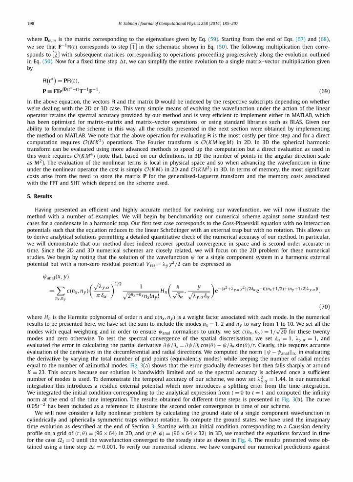
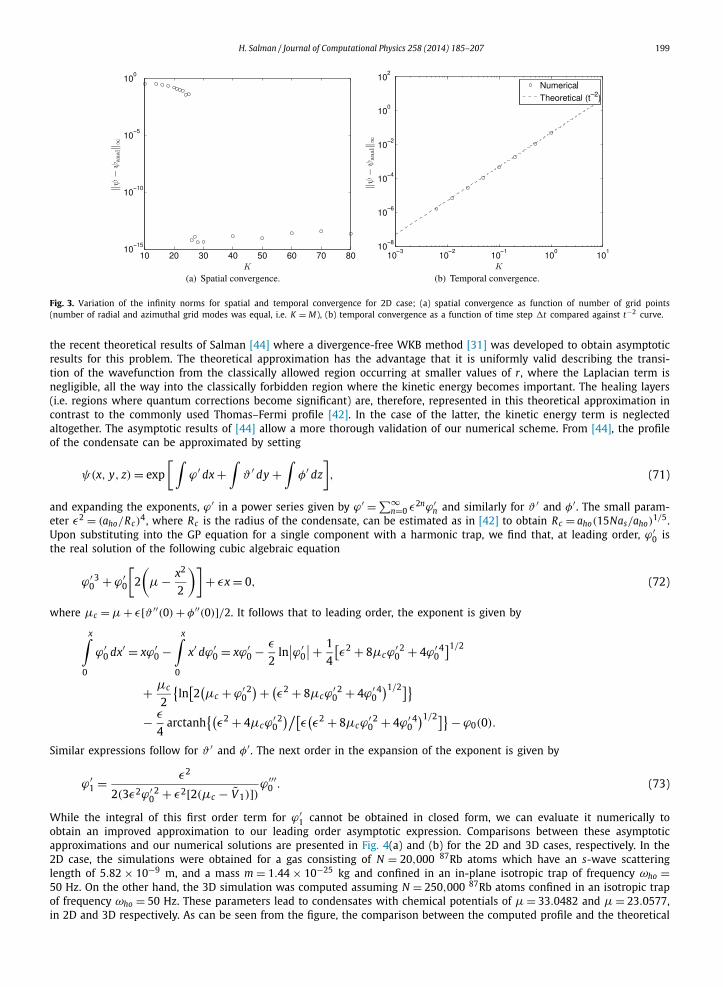
modes and zero otherwise. To test the spectral convergence of the spatial discretisation, we set δα = 1, λy,α = 1, andevaluated the error in calculating the partial derivative ∂ψ/∂x = ∂ψ/∂r cos(θ) − ψ/∂θ sin(θ)/r. Clearly, this requires accurateevaluation of the derivatives in the circumferential and radial directions. We computed the norm ‖ψ −ψanal‖∞ in evaluatingthe derivative by varying the total number of grid points (equivalently modes) while keeping the number of radial modesequal to the number of azimuthal modes. Fig. 3(a) shows that the error gradually decreases but then falls sharply at aroundK = 23. This occurs because our solution is bandwidth limited and so the spectral accuracy is achieved once a sufficientnumber of modes is used. To demonstrate the temporal accuracy of our scheme, we now set λ2

y,α = 1.44. In our numericalintegration this introduces a residue external potential which now introduces a splitting error from the time integration.We integrated the initial condition corresponding to the analytical expression from t = 0 to t = 1 and computed the infinitynorm at the end of the time integration. The results obtained for different time steps is presented in Fig. 3(b). The curve0.05t−2 has been included as a reference to illustrate the second order convergence in time of our scheme.

We will now consider a fully nonlinear problem by calculating the ground state of a single component wavefunction incylindrically and spherically symmetric traps without rotation. To compute the ground states, we have used the imaginarytime evolution as described at the end of Section 3. Starting with an initial condition corresponding to a Gaussian densityprofile on a grid of (r, θ) = (96 × 64) in 2D, and (r, θ,φ) = (96 × 64 × 32) in 3D, we marched the equations forward in timefor the case Ωz = 0 until the wavefunction converged to the steady state as shown in Fig. 4. The results presented were ob-tained using a time step �t = 0.001. To verify our numerical scheme, we have compared our numerical predictions against


Fig. 3. Variation of the infinity norms for spatial and temporal convergence for 2D case; (a) spatial convergence as function of number of grid points(number of radial and azimuthal grid modes was equal, i.e. K = M), (b) temporal convergence as a function of time step �t compared against t−2 curve.

the recent theoretical results of Salman [44] where a divergence-free WKB method [31] was developed to obtain asymptoticresults for this problem. The theoretical approximation has the advantage that it is uniformly valid describing the transi-tion of the wavefunction from the classically allowed region occurring at smaller values of r, where the Laplacian term isnegligible, all the way into the classically forbidden region where the kinetic energy becomes important. The healing layers(i.e. regions where quantum corrections become significant) are, therefore, represented in this theoretical approximation incontrast to the commonly used Thomas–Fermi profile [42]. In the case of the latter, the kinetic energy term is neglectedaltogether. The asymptotic results of [44] allow a more thorough validation of our numerical scheme. From [44], the profileof the condensate can be approximated by setting

ψ(x, y, z) = exp

[∫ϕ′ dx +

∫ϑ ′ dy +

∫φ′ dz

], (71)

and expanding the exponents, ϕ′ in a power series given by ϕ′ = ∑∞n=0 ε2nϕ′

n and similarly for ϑ ′ and φ′ . The small param-eter ε2 = (aho/Rc)

4, where Rc is the radius of the condensate, can be estimated as in [42] to obtain Rc = aho(15Nas/aho)1/5.

Upon substituting into the GP equation for a single component with a harmonic trap, we find that, at leading order, ϕ′0 is

the real solution of the following cubic algebraic equation

ϕ′ 30 + ϕ′

0

[2

(μ − x2

2

)]+ εx = 0, (72)

where μc = μ + ε[ϑ ′′(0) + φ′′(0)]/2. It follows that to leading order, the exponent is given by

x∫0

ϕ′0 dx′ = xϕ′

0 −x∫

0

x′ dϕ′0 = xϕ′

0 − ε

2ln∣∣ϕ′

0

∣∣+ 1

4

[ε2 + 8μcϕ

′ 20 + 4ϕ′ 4

0

]1/2

+ μc

2

{ln[2(μc + ϕ′ 2

0

)+ (ε2 + 8μcϕ

′ 20 + 4ϕ′ 4

0

)1/2]}− ε

4arctanh

{(ε2 + 4μcϕ

′ 20

)/[ε(ε2 + 8μcϕ

′ 20 + 4ϕ′ 4

0

)1/2]}− ϕ0(0).

Similar expressions follow for ϑ ′ and φ′ . The next order in the expansion of the exponent is given by

ϕ′1 = ε2

2(3ε2ϕ′ 20 + ε2[2(μc − V 1)])

ϕ′′′0 . (73)

While the integral of this first order term for ϕ′1 cannot be obtained in closed form, we can evaluate it numerically to

obtain an improved approximation to our leading order asymptotic expression. Comparisons between these asymptoticapproximations and our numerical solutions are presented in Fig. 4(a) and (b) for the 2D and 3D cases, respectively. In the2D case, the simulations were obtained for a gas consisting of N = 20,000 87Rb atoms which have an s-wave scatteringlength of 5.82 × 10−9 m, and a mass m = 1.44 × 10−25 kg and confined in an in-plane isotropic trap of frequency ωho =50 Hz. On the other hand, the 3D simulation was computed assuming N = 250,000 87Rb atoms confined in an isotropic trapof frequency ωho = 50 Hz. These parameters lead to condensates with chemical potentials of μ = 33.0482 and μ = 23.0577,in 2D and 3D respectively. As can be seen from the figure, the comparison between the computed profile and the theoretical


Fig. 4. Comparison of analytical and numerical condensate profiles for (a) 2D condensate, (b) 3D condensate, with and without a single quantised vortexlocated at the centre of the condensate for a system consisting of 20,000 87Rb atoms in an isotropic trap with ωho = 50 Hz.

result is excellent over the entire interval of the computational domain. We note that while some discrepancies exist nearthe edge of the condensate, this stems from the asymptotic approximation used to obtain our theoretical results. Indeed,by retaining the correction from the next order in the asymptotic expansion, we see that the numerical predictions andtheoretical results become indistinguishable.

The results presented in Fig. 4 demonstrate our scheme correctly predicts the ground state for the l = 0 modes. However,a key feature that must be benchmarked is that the scheme works correctly for l �= 0. This would then demonstrate that thetime marching scheme given by Eqs. (67)–(68) which rely on the use of the transform matrices T,F between different gridpoints yields the correct results. For this purpose, we have repeated a similar ground state computation as in the above casewith Ωz = 0 but now we phase imprint a vortex onto our condensate solutions that are located at the centre of the traps.The vortex profile is obtained from the Padé approximant evaluated by Berloff [14]. After relaxing the solution through animaginary time evolution of the GP equations, we find that the system settles into a metastable state consisting of a singlevortex located at the centre of the traps. The vortex breaks the spherical symmetry thereby allowing us to check that thetransfer matrices have been implemented correctly. A ground state computation for this problem is also shown in Fig. 4(a)and (b) for both 2D and 3D cases. The characteristic dip in the densities of the condensates at the centres of the trapsseen for the rotating cases are indicative of the signature of a quantised vortex. As in the non-rotating case, an asymptoticapproximation for the condensates using the divergence-free WKB method was also derived in [44]. This is now given by

ϕ(r) = r log(r)ϕ′ + rϕ′

2− 1

2ε log

(∣∣rϕ′ + ε∣∣)− 1

2log

(∣∣∣∣μrϕ′ −√(rϕ′)4 + (μ2 − 2ε2)(rϕ′)2 + ε4

rϕ′ − ε

∣∣∣∣)

rϕ′

− ε

2R{

arctan

(μ[(rϕ′)2 + ε2]

2ε√

(rϕ′)4 + (μ2 − 2ε2)(rϕ′)2 + ε4

)}

+ μ

4log

(∣∣∣∣μ2

2− ε2 + (

rϕ′)2 +√(

rϕ′)4 + (μ2 − 2ε2

)(rϕ′)2 + ε4

∣∣∣∣)

,

where R(·) denotes the real part. As before, we observe excellent agreement between the theory and the numerical results.These benchmarks clearly demonstrate the correct implementation of our numerical scheme.

We will now proceed by demonstrating our scheme for ground state computations of a vortex lattice beginning froma condensate without any vortices under the influence of rotation. We solved Eq. (2) for a single component in a toroidaltrap by setting γ12 = 0. As before, a grid of (r, θ) = (96 × 64) was used and the equation was integrated in imaginarytime with �t = 0.001 and for two different rotation speeds corresponding to Ω = 0.225 and Ω = 0.5 which are based onthe parameters used in [2]. To break the symmetry and simulate the formation of a vortex lattice, we used a numericallycomputed ground state profile without vortices and imposed small perturbations on the condensate density. After evolvingthe system in time, we observed the formation of quantised vortices which settled into the patterns shown in Figs. 5 and 6.For slow rotation speeds, the vortices enter from the edges of the condensate and adopt a steady pattern. For faster rotationspeeds, the toroidal trap modifies the density profile of the condensate to a ring-shaped condensate with vortices uniformlydistributed along the azimuthal direction. While our results are similar to the results presented in [2], we neverthelessnotice some differences from their results (see Figs. 4b and 4d in [2]). These differences are possibly caused by the breakingof the azimuthal symmetry by the Cartesian grid used in [2]. Moreover, since the ground states are not necessarily unique,or may be nearly degenerate in the sense that several metastable states can be located very close to the ground state of thesystem, it is easy for the system to converge to slightly different solutions even for the same set of parameters.

Having illustrated our method for a one component system, we will now consider a two-component condensate. Ithas been shown that for components consisting of different atomic species, the difference in the atomic masses between


Fig. 5. Density and phase contour plots of a rotating condensate in an isotropic harmonic trap with γ (2D) = 500, λtr = 60, ltr = 0.1,Ωz = 0.225.

Fig. 6. Density and phase contour plots of a rotating condensate in an isotropic harmonic trap with γ (2D) = 500, λtr = 60, ltr = 0.1,Ωz = 0.5.

Fig. 7. Vortex lattices in each component together with plot of superposition of vortex lattices in both components for m1/m2 = 1.0.

the species can lead to a ground state in which the vortices are distributed differently in each component from the casewhen the components are assumed to have equal masses (e.g. in the case of a system made up of atoms in differenthyperfine states). The 2D vortex lattices in this case were first predicted in the work of [10] and later illustrated withnumerical simulations of the GP equation in [11]. However, as discussed throughout the paper, this case raises additionalchallenges to simulate with the generalised-Laguerre basis functions since the collocation points for each component donot coincide under such situations. We will, therefore, present simulations for a two-component condensate to demonstratethat the method we have developed leads to an accurate and efficient scheme that can be used to simulate such systems.In direct analogy with the results of [11], we have considered a two-component condensate with γ

(2D)11 = 2 × 104 and

γ(2D)

12 = −2γ(2D)

11 /3. The number of atoms was assumed to be equal in each component so that N1 = N2 and the angularrotation was set to Ωz = 0.9. Two different mass ratios were considered, the first with m1/m2 = 1.0 and the second withm1/m2 = 1.4. After integrating the equations in imaginary time on a grid consisting of (96 × 128) collocation points in(r, θ), with a time step of �t = 0.002, we obtained the solutions presented in Figs. 7 and 8. As can clearly be seen, for amass ratio of unity the vortex lattices in both components are locked together as expected. However, when the mass ratiois increased from 1.0 to 1.4, and the vortex lattice obtained in the former case is relaxed under further imaginary timeevolution, we observe that the vortex lattices remain locked together within the inner regions of the condensate. On theouter regions, the vortices necessarily occupy different positions in space which is fully consistent with the analysis andresults presented in [10,11]. The numerical simulations we have presented, therefore verify our numerical scheme even forthe case of a multi-component condensate with different mass ratios.


Fig. 8. Vortex lattices in each component together with plot of superposition of vortex lattices in both components for m1/m2 = 1.4.

Fig. 9. Density of a 2D condensate with a precessing quantised vortex located off-centre at a radius r = 2 for a system consisting of 20,000 87Rb atoms inan isotropic trap with ωho = 50 Hz, and λtr = 0,Ωz = 0.

Fig. 10. Conservation of L2 and energy norms for case of a 2D system consisting of 20,000 87Rb atoms in an isotropic trap with ωho = 50 Hz, andλtr = 0,Ωz = 0.

Having demonstrated that our method correctly reproduces the ground state properties of a one and two-componentsystem, we will now focus on time-dependent simulations of the GP system of equations. We begin by considering theprecession of a single quantised vortex imprinted onto the ground state density of a non-rotating 2D condensate withparameters similar to those considered above for the results presented in Fig. 4(a). The ground state is computed numericallyon a grid of 96 × 64 grid points in the (r, θ) directions, respectively, using the imaginary time evolution as described above.The vortex is then imprinted at (r, θ) = (2,0) by setting ψ = ψgsψvortex where ψgs is the numerically computed groundstate and ψvortex is set to correspond to a vortex according to the specification given in [14] but where the core radius hasbeen modified to account for the different condensate density at the position of the vortex. Using this initial condition, thewavefunction is evolved forward in time using the second order Strang splitting with a time step of �t = 0.0005. As can beseen in Fig. 9, the vortex precesses around the centre of the trap at a fixed radius as expected. Throughout the evolution,we have tracked both the L2 norm of ψ (i.e. the total number of particles, N) and the total energy given by H . As can beseen in Fig. 10(a) and (b), both quantities are conserved to a high degree of accuracy throughout the time of integration.However due to our need to truncate the modes based on a uniform energy cut-off, our scheme does not conserve thesequantities at the discretised level thereby resulting in the small variations that are seen in the figures.


Fig. 11. Time evolution of density and phase contours for two-component condensate with Ωz = 0, λtr = 0. The initial phase imprinted on the secondcomponent causes the second component to rotate relative to the first component and gives rise to the onset of a Kelvin–Helmholtz instability.

To further illustrate the capability of our numerical scheme, we have also performed a time-dependent simulation of theonset of the Kelvin–Helmholtz instability in a trapped 2D two-component condensate as considered by [48]. This test caseprovides an ideal benchmark problem permitting both a qualitative and quantitative evaluation of the correct implementa-tion of the scheme. We will use similar parameters to the study of Suzuki et al. in which an atomic condensate consistingof a total of N = 1.63 × 106 23Na atoms was modelled. We assumed the gas is made up of atoms in two different hyperfinestates that make up the two components with an equal population in each component. The gas is taken to be trapped in anaxisymmetric harmonic potential where the radial and axial trap frequencies are ω⊥ = 2π × 80 Hz and ωz = 2π × 4 kHz,respectively. The strong trapping in the z direction effectively freezes out the dynamics in this direction allowing us toconsider effectively two-dimensional dynamics in our simulations. Following [48], we have set the scattering lengths toa11 � 53.4aB , a12 = a22 � 54.2aB with aB being the Bohr radius. These parameters favour a phase-separated two-componentcondensate. Using these parameters, we prepare the initial state of the system by first integrating the equations forwardin imaginary time subject to the constraint on the number of particles using the same approach to that described above.Since our parameters lead to phase separation of the two components and a22 > a11, we find that the ground state con-sists of component 1 occupying the centre of the trap and is surrounded by component 2 in the form of a ring-shapedcondensate as shown in Fig. 11 for t = 0. After computing the ground states, we imprint a phase on the wavefunction ofthe second component so that ψ2 = |ψ2,gs|ein2θ where ψ2,gs denotes the ground state wavefunction for the second com-ponent. We set n2 = 18 which produces an overall rotation in the second component. Our initial condition, that we usefor the forward time integration, now consists of two phase-separated components with a circular interface and with theouter component rotating relative to the inner component. This provides the key ingredients necessary for the onset of theKelvin–Helmholtz instability. To break the axisymmetry, we add small numerical noise to our wavefunctions in the formof ψnoise(r, θ) = 0.001ei2π Rn(r,θ) where Rn(r, θ) is a randomly sampled function with a uniform distribution. These newwavefunctions are used as the initial conditions for the density and the phase and is shown in Fig. 11 for t = 0. The initialcondition is integrated forward in time using our numerical scheme for the 2D two-component condensate with a timestep of �t = 0.0001. We observe that after some time, a Kelvin–Helmholtz instability develops at the interface between thetwo components. As time progresses, the instability grows leading to the formation of well defined vortices at the interface.Our results are in perfect qualitative agreement with those presented by Suzuki et al. As a further quantitative check of ourresults, we note that nine vortices are produced at the interface in our simulations which are in direct agreement with themost unstable azimuthal mode as predicted from a linear stability analysis in [48]. We therefore conclude that our methodreproduces the correct temporal behaviour for this case.

As an illustrative example of our 3D scheme, we will present time-dependent simulations of a 3D condensate. We beginby repeating the precessing vortex problem in 3D using γ (3D) = 1.2 × 104 and a grid of 96 × 64 × 32 points in the (r, θ,φ)

directions respectively. We begin by imprinting a single quantised vortex aligned along the z direction at r = 2 and θ = 0.This initial condition is then integrated forward in time using a time step of �t = 0.005. As for the 2D case, the vortexprecesses around the centre of the trap as indicated by the final vortex position shown in Fig. 12(a). The 3D isometric viewof the vortex shown in the figure clearly depicts the nature of these topological defects within the condensate. As for the 2D


Fig. 12. Precessing vortex in a 3D condensate consisting of 20,000 87Rb atoms in an isotropic trap with ωho = 50 Hz, and λtr = 0,Ωz = 0: (a) isosurfacecorresponding to |ψ | = 0.025 showing nature of single quantised vortex as a topological defect precessing within the condensate for {γ (3D) = 12,000,

λtr = 0,Ωz = 0}. The isosurface contouring is given by the function√

r where r is the radius measured from the centre of the condensate and thereforereflects the distance that different isosurfaces are located from the centre of the trap; (b) Variation of normalised L2 norm of condensate wavefunctionwith time; (b) Variation of normalised energy with time.

Fig. 13. Cross-sectional density profiles of turbulent condensate state for case with {γ (3D) = 12,000, λtr = 0,Ωz = 0}.

Fig. 14. Condensate isosurface corresponding to |ψ | = 0.025 showing relaxation of turbulent vortex tangle with time for {γ (3D) = 12,000, λtr = 0,Ωz = 0}.The isosurface contouring is given by the function

√r where r is the radius measured from the centre of the condensate and therefore reflects the distance

that different isosurfaces are located from the centre of the trap.

case, we tracked the total number of particles and Hamiltonian with time as shown in Fig. 12(b), (c). As before, we observethat both quantities are conserved to a high accuracy by our numerical method.

We end by simulating the evolution of a vortex tangle in an atomic Bose–Einstein condensate. We prescribe our initialcondition by setting ψ = ψgsei2π Rn(r,θ,φ) where, as before, Rn(r, θ,φ) is a randomly sampled function with a uniform dis-tribution. We first relaxed this initial condition through an imaginary time evolution over an interval of t = 0.1 units usinga time step �t = 0.00002. This has the effect of producing a system at intermediate energies consisting of quantised vortexexcitations superimposed on top of a condensate. Cross-sections of the resulting condensate density are shown in Fig. 13.The corresponding 3D view depicting the vortex tangle that is indicative of a condensate in a turbulent state is shown inFig. 14. Using the initial condition shown in Fig. 13(a) and Fig. 14(a), we evolved the wavefunction under the conservative


GP equation. The resulting evolution is shown at different times in the figure and illustrates how the tangle relaxes withtime. This scenario in which vortices evolve and reconnect and ultimately decay is reminiscent of similar simulations carriedout by Berloff and Svistunov [13] but for a homogeneous system.

6. Conclusions

We have presented a fully realisable implementation of a numerical scheme based on generalised-Laguerre polynomi-als with Fourier or spherical harmonics for the solution of the GP multi-component system of equations confined withina harmonic and toroidal trapping potential for 2D and 3D condensates, respectively. A key issue that arises when usinggeneralised-Laguerre polynomials is how to truncate the modes corresponding to different angular wavenumbers. We haveshown that a truncation based on the energy spectrum of the linear operator leads to a self-consistent and accurate nu-merical scheme. An efficient implementation was accomplished by reducing the pseudospectral scheme to matrix–vectoroperations that could easily be implemented using MATLAB. An important feature of the discretisation presented is the im-proved accuracy one achieves when combined with an operator-splitting method for the time integration of the governingequation in comparison to methods that have previously been presented in the literature.

Using recently derived theoretical results for the ground state properties of a Bose gas in a harmonic trap with andwithout rotation, we have been able to demonstrate excellent agreement with our numerical results obtained using ourscheme. Furthermore, in contrast to previous work, our approach circumvents the difficulties that arise from having differentLaguerre–Lobotto quadrature points for generalised-Laguerre polynomials that correspond to different angular/centrifugalnumber. This allows us to apply our method to fully 2D and 3D numerical simulations resulting in a fully general andaccurate scheme by solving the GP equation in the most natural coordinate system for describing the geometry of BECs thatare typically found in a number of experiments. We have demonstrated the full applicability of the method by studying thetime-dependent dynamics of vortex lattice formation in 2D, and the motion of a quantised vortex in a spherical BEC.

Given that the scheme we have presented uses a single-particle basis allowing direct control over the cut-off of theenergy spectrum, the method will be ideal for use with finite temperature models of BECs. In modelling finite temperatureeffects, this level of numerical control is essential in order to recover the correct equilibrium properties of the system[44,16]. The scheme we have presented is, therefore, likely to find applications in these other areas of atomic physics wherethermodynamics and nonequilibrium condensate growth form an important area of research. In addition, the modelling ofvortex dynamics that we have focused on in this work is known to be of essence to an understanding of the problem ofsuperfluid turbulence and provides another promising area of application of the numerical scheme presented here.

Appendix A. Non-dimensionalisation of the governing equations of motion

We are interested in modelling the dynamics of a weakly interacting one- or two-component Bose-condensed gas atzero temperature (T = 0). In the presence of a confining external potential, the dynamics of the condensate wavefunctionsψα(x, t), where α = 1,2 for the two different components, can be described by two coupled Gross–Pitaevskii (GP) [40]equations which are given by

ih∂ψ1(x, t)

∂t= −h2

2m1∇2ψ1(x, t) + V 1(x)ψ1(x, t) + U (d)

11

∣∣ψ1(x, t)∣∣2ψ1(x, t)

+ U (d)12

∣∣ψ2(x, t)∣∣2ψ1(x, t) − ihΩ · x × ∇ψ1(x, t),

ih∂ψ2(x, t)

∂t= −h2

2m2∇2ψ2(x, t) + V 2(x)ψ2(x, t) + U (d)

22

∣∣ψ2(x, t)∣∣2ψ2(x, t)

+ U (d)21

∣∣ψ1(x, t)∣∣2ψ2(x, t) − ihΩ · x × ∇ψ2(x, t), (A.1)

where d denotes the number of spatial dimensions, and x ∈ Rd with x = (x, y) in 2D and x = (x, y, z) in 3D, respectively. In

addition, h is the reduced Planck’s constant, V 1(x) and V 2(x) are the external trapping potentials, U (d)αβ are the interatomic

and intra-atomic interaction coefficients, and Ω is the angular rotation vector. We note that the interatomic interactionsmust satisfy the condition U (d)

12 = U (d)21 . For components corresponding to atoms in two different hyperfine states, m1 = m2.

However, for different atomic species, mα would correspond to the atomic mass of each species. In this work, we willexclusively consider the case of a harmonic trapping potential with a possibility of a Gaussian central potential in whichcase

Vα(x) =

⎧⎪⎨⎪⎩

12 mα(ω2

x,αx2 + ω2y,α y2) + mαω2

tr,α exp(−2(x2+y2)

L2tr,α

) in 2D,

12 mα(ω2

x,αx2 + ω2y,α y2 + ω2

z,αz2) + mαω2tr,α exp(

−2(x2+y2)

L2tr,α

) in 3D,(A.2)

with ωx,α , ωy,α , ωz,α being the harmonic trap frequencies for the two components in the x, y, and z directions respectively.The strength of the Gaussian potential located at the centre is determined by the toroidal trapping frequency ωtr,α , and thewidth is characterised by Ltr,α . The above equation is then supplemented by the boundary conditions


ψα → 0 as |x| → ∞, (A.3)

which is a consequence of the harmonic trapping potentials Vα(x) → ∞ as |x| → ±∞.The interaction parameters U (d)

αβ are defined differently in 2D and 3D. In 3D, U (3)αβ = 2π h2as,αβ(mα + mβ)/mαmβ and are

related to the s-wave scattering lengths as,αβ which can typically be varied in experiments through the use of Feshbach

resonance [40]. The interaction parameters in 2D are then given by U (2)αβ = U (3)

αβ(mαωz,α/(2π h))1/2. The GP system of equa-tions has a number of important conserved quantities including the total number of particles in each component and thetotal energy (Hamiltonian) which are given respectively by [25]

Nα =∫Rd

∣∣ψα(x, t)∣∣2 ddx, (A.4)

H =∫Rd

[2∑

α=1

(h2

2mα

∣∣∇ψα(x, t)∣∣2 + Vα(x)

∣∣ψα(x, t)∣∣2 + U (d)

α,α

2

∣∣ψα(x, t)∣∣4)+ U (d)

12

∣∣ψ1(x, t)∣∣2∣∣ψ2(x, t)

∣∣2]ddx

− ih

∫Rd

[2∑

α=1

ψ∗αΩ · x × ∇ψα(x, t)

]ddx. (A.5)

We will non-dimensionalise the above equations using the oscillator length scale (aho = √h/(m1ωho)), and the oscillator

frequency given by ωho = (ωx,1ωy,1ωz,1)1/3 in 3D, and ωho = (ωx,1ωy,1)

1/2 in 2D. Then rescaling space and time such that

t → t/ωho, x → xaho, (A.6)

and normalising the wavefunctions to unity by setting ψα → √Nαψα , we obtain

i∂ψ1(x, t)

∂t=

[−1

2∇2 + V 1(x) + γ

(d)11

∣∣ψ1(x, t)∣∣2 + γ

(d)12

∣∣ψ2(x, t)∣∣2 − ix · Ω × ∇

]ψ1(x, t),

i∂ψ2(x, t)

∂t=

[−δ

2∇2 + 1

δV 2(x) + γ

(d)22

∣∣ψ2(x, t)∣∣2 + γ

(d)21

∣∣ψ1(x, t)∣∣2 − ix · Ω × ∇

]ψ2(x, t), (A.7)

with

Vα(x) =

⎧⎪⎨⎪⎩

12 (λ2

x,αx2 + λ2y,α y2) + λtr,α exp(

−2(x2+y2)

l2tr,α) in 2D,

12 (λ2

x,αx2 + λ2y,α y2 + λ2

z,αz2) + λtr,α exp(−2(x2+y2)

l2tr,α) in 3D.

(A.8)

In Eq. (A.7), γ(3)αβ = 2π Nβas,αβ(1 + mα/mβ)δα/aho in 3D whereas γ

(2)αβ = γ

(3)αβ aho(mαωz,α/2π h)1/2 in 2D, λx,α = ωx,α/ωho ,

λy,α = ωy,α/ωho , λz,α = ωz,α/ωho , λtr,α = ωtr,α/ωho , Ω = Ω/ωho , ltr,α = Ltr,α/aho , δ = m1/m2 > 1 (i.e. we set componentone to correspond to the gas with the larger of the two masses). For later convenience, we have introduced the parameterδα such that δ1 = 1 and δ2 = δ. These equations can be solved subject to the initial conditions ψα(x,0) = ψ0,α(x).

In the limit where the harmonic trap oscillator frequency in one direction becomes significantly strong, the dynamics ofthe condensate will be severely restricted to occur essentially on the plane spanned by the vectors normal to that direction.Without loss of generality, we can take this direction to be along the z-coordinate axis, such that ωz � ωx,ωy . In this casethe dynamics reduces to motion on the x–y plane. Moreover, since we will be interested in simulating rotating condensateswe can take without loss of generality Ω = (0,0,Ωz). We, will therefore consider cases where the respective equations willbe solved in 2D as well as 3D. In the former, we will work with a polar (r, θ) coordinate system whereas in the latter, wewill revert to a spherical coordinate system denoted by (r, θ,φ). After re-expressing our wavefunctions in terms of polar(ψ(x, t) → ψ(r, t) ≡ ψ(r, θ, t)), and spherical (ψ(x, t) → ψ(r, t) ≡ ψ(r, θ,φ, t)) coordinates, we recover Eqs. (2) and (5),respectively.

References

[1] M. Abramowitz, I.A. Stegun, Handbook of Mathematical Functions with Formulas, Graphs, and Mathematical Tables, Dover Publications, New York,1972.

[2] A. Aftalion, P. Mason, Rotation of a Bose–Einstein condensate held under a toroidal trap, Phys. Rev. A 81 (2010) 023607.[3] M.H. Anderson, J.R. Ensher, M.R. Matthews, C.E. Wieman, E.A. Cornell, Observation of Bose–Einstein condensation in a dilute atomic vapor, Science

269 (5221) (1995) 198–201.[4] G.E. Astrakharchik, L.P. Pitaevskii, Motion of a heavy impurity through a Bose–Einstein condensate, Phys. Rev. A 70 (2004) 013608.[5] W. Bao, D. Jaksch, An explicit unconditionally stable numerical method for solving damped nonlinear Schrödinger equations with a focusing nonlin-

earity, SIAM J. Numer. Anal. 41 (2003) 1406–1426.

http://refhub.elsevier.com/S0021-9991(13)00677-3/bib416272616D6F7769747A3732s1

http://refhub.elsevier.com/S0021-9991(13)00677-3/bib416272616D6F7769747A3732s1

http://refhub.elsevier.com/S0021-9991(13)00677-3/bib416674616C696F6E3130s1

http://refhub.elsevier.com/S0021-9991(13)00677-3/bib416E646572736F6E3935s1

http://refhub.elsevier.com/S0021-9991(13)00677-3/bib416E646572736F6E3935s1

http://refhub.elsevier.com/S0021-9991(13)00677-3/bib41737472616B6861726368696B3034s1

http://refhub.elsevier.com/S0021-9991(13)00677-3/bib42616F3033s1



[6] W. Bao, J. Shen, A fourth-order time-splitting Laguerre–Hermite pseudospectral method for Bose–Einstein condensates, SIAM J. Sci. Comput. 26 (6)(2005) 2010–2028.

[7] W. Bao, J. Shen, A generalized-Laguerre–Hermite pseudospectral method for computing symmetric and central vortex states in Bose–Einstein conden-sates, J. Comput. Phys. 227 (2008) 9778–9793.

[8] W. Bao, H. Li, J. Shen, A generalized-Laguerre–Fourier–Hermite pseudospectral method for computing the dynamics of rotating Bose–Einstein conden-sates, SIAM J. Sci. Comput. 31 (2009) 3685–3711.

[9] W. Bao, Y. Cai, Mathematical theory and numerical methods for Bose–Einstein condensates, Kinet. Relat. Models 6 (2013) 1–135.[10] R. Barnett, G. Refael, M. Porter, H.P. Büchler, Vortex lattice locking in rotating two-component Bose–Einstein condensates, New J. Phys. 10 (2008)

043030.[11] R. Barnett, E. Chen, G. Refael, Vortex synchronization in Bose–Einstein condensates: A time-dependent Gross–Pitaevskii equation approach, New J. Phys.

12 (2010) 043004.[12] D. Baye, P.-H. Heenen, Generalised meshes for quantum mechanical problems, J. Phys. A, Math. Gen. 19 (1986) 2041–2059.[13] N.G. Berloff, B.V. Svistunov, Scenario of strongly non-equilibrated Bose–Einstein condensation, Phys. Rev. A 66 (2002) 013603.[14] N.G. Berloff, Padé approximations of solitary wave solutions of the Gross–Pitaevskii equation, J. Phys. A, Math. Gen. 37 (2004) 1617–1632.[15] P.B. Blakie, Numerical method for solving the projected Gross–Pitaevskii equation, Phys. Rev. E 78 (2008) 026704.[16] P.B. Blakie, A.S. Bradley, M.J. Davis, Dynamics and statistical mechanics of ultra-cold Bose gases using c-field techniques, Adv. Phys. 57 (2008) 363–455.[17] A.G. Borisov, Solution of the radial Schrödinger equation in cylindrical and spherical coordinates by mapped Fourier transform algorithms, J. Chem.

Phys. 114 (18) (2001) 7770–7777.[18] J.P. Boyd, C. Rangan, P.H. Bucksbaum, Pseudospectral method on a semi-infinite interval with application to a hydrogen atom: A comparison of the

mapped Fourier-sine method with Laguerre series and rational Chebyshev expansions, J. Comput. Phys. 188 (2003) 56–74.[19] C.C. Bradley, C.A. Sackett, J.J. Tollett, R.G. Hulet, Evidence of Bose–Einstein condensation in an atomic gas with attractive interactions, Phys. Rev. Lett.

75 (9) (1995) 1687–1690.[20] A.S. Bradley, C.W. Gardiner, M.J. Davis, Bose–Einstein condensation from a rotating thermal cloud: Vortex nucleation and lattice formation, Phys. Rev.

A 77 (2008) 033616.[21] P.J. Channell, C. Scovel, Symplectic integration of Hamiltonian systems, Nonlinearity 3 (1990) 231–259.[22] G.C. Corey, Pseudospectral method for solving the time-dependent Schrödinger equation in spherical coordinates, J. Chem. Phys. 97 (6) (1992)

4115–4126.[23] J.R. Discoll, D. Healy, Computing Fourier transforms and convolutions on the 2-sphere, Adv. Appl. Math. 15 (1994) 202.[24] M. Edwards, P.A. Ruprecht, K. Burnett, R.J. Dodd, C.W. Clark, Collective excitations of atomic Bose–Einstein condensates, Phys. Rev. Lett. 77 (1996)

1671–1674.[25] A.L. Fetter, Rotating trapped Bose–Einstein condensates, Rev. Mod. Phys. 81 (2009) 647.[26] B. Fornberg, A Practical Guide to Pseudospectral Methods, 1998.[27] V.M. Pérez-García, X. Liu, Numerical methods for the simulation of trapped nonlinear Schrödinger systems, Appl. Math. Comput. 144 (2003) 215–235.[28] D. Gottlieb, A. Orszag, Numerical Analysis of Spectral Methods: Theory and Applications, 1977.[29] E.P. Gross, Structure of a quantized vortex in boson systems, Nuovo Cimento 20 (3) (May 1961) 454–457.[30] M.R. Hermann, J.A. Fleck Jr., Split-operator spectral method for solving the time-dependent Schrödinger equation in spherical coordinates, Phys. Rev. A

38 (12) (1988) 6000–6012.[31] T. Hyouguchi, S. Adachi, M. Ueda, Divergence-free WKB method, Phys. Rev. Lett. 88 (2002) 170404.[32] S. Jiang, L. Greengard, Efficient representation of nonreflecting boundary conditions for the time-dependent Schrödinger equation in two dimensions,

Commun. Pure Appl. Math. 61 (2) (2008) 261–288.[33] D.S. Jin, J.R. Ensher, M.R. Matthews, C.E. Wieman, E.A. Cornell, Collective excitations of a Bose–Einstein condensate in a dilute gas, Phys. Rev. Lett. 77

(1996) 420–423.[34] K. Kasamatsu, M. Tsubota, Quantized vortices in atomic Bose–Einstein condensates, in: M. Tsubota (Ed.), Prog. Low Temp. Phys., Quantum Turbul.,

vol. XVI, Elsevier, 2009.[35] P.G. Kevrekidis, D.J. Frantzeskakis, R. Carretero-González (Eds.), Emergent Nonlinear Phenomena in Bose–Einstein Condensates: Theory and Experiment,

Springer-Verlag, 2008.[36] R.I. McLachlan, R.W. Quispel, Splitting methods, Acta Numer. 11 (2002) 341–434.[37] R.I. McLachlan, R.W. Quispel, Geometric integrators for ODEs, J. Phys. A, Math. Gen. 39 (2006) 5251–5285.[38] G.M. Muslu, H.A. Erbay, Higher-order split-step Fourier schemes for the generalized nonlinear Schrödinger equation, Math. Comput. Simul. 67 (2005)

581–595.[39] D. Pathria, J.LL. Morris, Pseudo-spectral solution of nonlinear Schrödinger equations, J. Comput. Phys. 87 (1990) 108–125.[40] C.J. Pethick, H. Smith, Bose–Einstein Condensation in Dilute Gases, Cambridge University Press, 2008.[41] L.P. Pitaevskii, Vortex lines in an imperfect Bose gas, Zh. Eksp. Teor. Fiz. 40 (1961) 646–649 (in Russian); Sov. Phys. JETP 13 (1961) 451–454 (in English).[42] L.P. Pitaevskii, S. Stringari, Bose–Einstein Condensation, Clarendon, Oxford, 2003.[43] N.P. Proukakis, B. Jackson, Finite-temperature models of Bose–Einstein condensation, J. Phys. B, At. Mol. Opt. Phys. 41 (2008) 203002.[44] H. Salman, Approximating steady states in equilibrium and nonequilibrium condensates, Phys. Rev. A 85 (2012) 063622.[45] J. Shen, Stable and efficient spectral methods in unbounded domains using Laguerre functions, SIAM J. Numer. Anal. 38 (4) (2000) 1113–1133.[46] T. Sørevik, T. Birkeland, G. Okša, Numerical solution of the 3D time dependent Schrödinger equation in spherical coordinates: Spectral basis and effects

of split-operator technique, J. Comput. Appl. Math. 225 (2009) 56–67.[47] G. Strang, On the construction and comparison of difference schemes, SIAM J. Numer. Anal. 5 (1968) 506–517.[48] N. Suzuki, H. Takeuchi, K. Kasamatsu, M. Tsubota, H. Saito, Crossover between Kelvin–Helmholtz and counter-superflow instabilities in two-component

Bose–Einstein condensates, Phys. Rev. A 82 (2010) 063604.[49] T.R. Taha, M.J. Ablowitz, Analytical and numerical aspects of certain nonlinear evolution equations. II. Numerical nonlinear Schrödinger equation,

J. Comput. Phys. 55 (1984) 203–230.[50] J.A.C. Weideman, B.M. Herbst, Split-step methods for the solution of the nonlinear Schrödinger equation, SIAM J. Numer. Anal. 23 (3) (1986) 485–507.








http://refhub.elsevier.com/S0021-9991(13)00677-3/bib4261726E6574743038s1




http://refhub.elsevier.com/S0021-9991(13)00677-3/bib426179653836s1

http://refhub.elsevier.com/S0021-9991(13)00677-3/bib4265726C6F66663032s1

http://refhub.elsevier.com/S0021-9991(13)00677-3/bib4265726C6F66663034s1

http://refhub.elsevier.com/S0021-9991(13)00677-3/bib426C616B69653038s1

http://refhub.elsevier.com/S0021-9991(13)00677-3/bib426C616B69653038726576s1

http://refhub.elsevier.com/S0021-9991(13)00677-3/bib426F7269736F763031s1

http://refhub.elsevier.com/S0021-9991(13)00677-3/bib426F7269736F763031s1



http://refhub.elsevier.com/S0021-9991(13)00677-3/bib427261646C65793935s1




http://refhub.elsevier.com/S0021-9991(13)00677-3/bib4368616E6E656C6C3930s1



http://refhub.elsevier.com/S0021-9991(13)00677-3/bib446973636F6C6C3934s1




http://refhub.elsevier.com/S0021-9991(13)00677-3/bib466F726E626572673938s1


http://refhub.elsevier.com/S0021-9991(13)00677-3/bib476F74746C6965623737s1


http://refhub.elsevier.com/S0021-9991(13)00677-3/bib4865726D616E6E3838s1

http://refhub.elsevier.com/S0021-9991(13)00677-3/bib4865726D616E6E3838s1


http://refhub.elsevier.com/S0021-9991(13)00677-3/bib4A69616E673038s1




http://refhub.elsevier.com/S0021-9991(13)00677-3/bib4B6173616D617473753039s1


http://refhub.elsevier.com/S0021-9991(13)00677-3/bib4B657672656B69646973426F6F6B3038s1

http://refhub.elsevier.com/S0021-9991(13)00677-3/bib4B657672656B69646973426F6F6B3038s1

http://refhub.elsevier.com/S0021-9991(13)00677-3/bib4D634C6163686C616E3032s1

http://refhub.elsevier.com/S0021-9991(13)00677-3/bib4D634C6163686C616E3036s1

http://refhub.elsevier.com/S0021-9991(13)00677-3/bib4D75736C753035s1

http://refhub.elsevier.com/S0021-9991(13)00677-3/bib4D75736C753035s1



http://refhub.elsevier.com/S0021-9991(13)00677-3/bib506974616576736B69693631s1

http://refhub.elsevier.com/S0021-9991(13)00677-3/bib506974616576736B69693033s1

http://refhub.elsevier.com/S0021-9991(13)00677-3/bib50726F756B616B69733038s1

http://refhub.elsevier.com/S0021-9991(13)00677-3/bib53616C6D616E3132s1


http://refhub.elsevier.com/S0021-9991(13)00677-3/bib536F726576696B3039s1

http://refhub.elsevier.com/S0021-9991(13)00677-3/bib536F726576696B3039s1


http://refhub.elsevier.com/S0021-9991(13)00677-3/bib53757A756B693130s1

http://refhub.elsevier.com/S0021-9991(13)00677-3/bib53757A756B693130s1



http://refhub.elsevier.com/S0021-9991(13)00677-3/bib57656964656D616E3836s1

a time-splitting pseudospectral method for the solution of the gross–pitaevskii equations using...

Documents