a three-dimensional field study of solute transport through unsaturated, layered, porous
TRANSCRIPT

University of Nebraska - LincolnDigitalCommons@University of Nebraska - Lincoln
Publications from USDA-ARS / UNL Faculty U.S. Department of Agriculture: AgriculturalResearch Service, Lincoln, Nebraska
1991
A Three-Dimensional Field Study of SoluteTransport Through Unsaturated, Layered, PorousMedia 2. Characterization of Vertical DispersionT. R. EllsworthUniversity of Illinois at Urbana-Champaign
W. A. JuryUniversity of California - Riverside
Follow this and additional works at: http://digitalcommons.unl.edu/usdaarsfacpub
Part of the Agricultural Science Commons
This Article is brought to you for free and open access by the U.S. Department of Agriculture: Agricultural Research Service, Lincoln, Nebraska atDigitalCommons@University of Nebraska - Lincoln. It has been accepted for inclusion in Publications from USDA-ARS / UNL Faculty by anauthorized administrator of DigitalCommons@University of Nebraska - Lincoln.
Ellsworth, T. R. and Jury, W. A., "A Three-Dimensional Field Study of Solute Transport Through Unsaturated, Layered, Porous Media2. Characterization of Vertical Dispersion" (1991). Publications from USDA-ARS / UNL Faculty. 498.http://digitalcommons.unl.edu/usdaarsfacpub/498

WATER RESOURCES RESEARCH, VOL. 27, NO. 5, PAGES 967-981, MAY 1991
A Three-Dimensional Field Study of Solute Transport Through Unsaturated, Layered, Porous Media
2. Characterization of Vertical Dispersion T. R. ELLSWORTH•
U.S. Salinity Laborator3.,, Riverside, California
W. A. JURY
Department of Soil and Environmental Science, University of Cah.'fornia, Riverside
Solute plumes were created in an unsaturated field soil with either flux application or by leaching an initial resident distribution (see Ellsworth et al., this issue). The spatial variance of the plumes initially increased with time between the soil surface and a depth of 2.5 m, within which the soil was a nearly structureless loamy sand. Below this depth, the plumes were observed to compress in the vertical direction as they moved into, and through, a region of subangular blocky structure and loam texture (between 2.5 and 4.0 m depth). As the solute moved below the layer of fine texture, the plume variance again increased with time. Using a transformed advection-dispersion equation description, two constant, field-averaged transport coefficients, V* and D}:, were determined in a scaled coordinate system from the moment equations. These two constant parameters were then used to predict the observed local, or plot scale, transport. Results indicate that the two constant parameters describe transport reasonably well at each plot site and over all sampling depths.
INTRODUCTION
The quest for an adequate description of downward chem- ical movement through unsaturated soil has been a major priority of soil and environmental scientists for many years. Early efforts at describing the transport process focused on characterizing movement under steady-state water flow through repacked soil columns whose lateral dimension was small compared to the vertical. Under such conditions, the advection-dispersion (or convection-dispersion) equation (ADE) with two constant coefficients (the velocity and longitudinal dispersion coefficient) became generally ac- cepted as the consensus model for describing transport of mobile, nonreactive tracers [Nielsen and Biggar, 1962]. However, the basis for this selection was usually the degree of agreement shown between the model and the effluent concentrations of solute in miscible displacement experi- ments, which cannot evaluate whether the dispersion param- eter in the model is constant without examining concentra- tions at different distances from the inlet end [Taylor, 1953].
Although early field studies of solute movement at the plot scale used the ADE to describe experimental observations [Miller et al., 1965; Warrick et al., 1971], data obtained from experiments conducted at a number of plots over large surface areas showed significant variation from one location to another in the values of the ADE coefficients required to match the model observations [Biggat and Nielsen, 1976; Van de Pol et al., 1977; Starr et al., 1978]. Furthermore, when the size of the solute inlet area was relatively large compared to the lateral dimension (as, for example, in an
•Now at Department of Agronomy, University of Illinois at Urbana-Champaign.
Copyright 1991 by the American Geophysical Union.
Paper number 91WR00190. 0043- !397/91/91WR-00190505.00
agricultural field), the apparent dispersion coefficient re- quired to fit the ADE model to the area-averaged data increased with distance from the inlet end [Butters and Jur3.,, 1989], (see also review by Gelhat et al. [1985]). This phe- nomenon, called the dispersion scale effect, has been ob- served repeatedly in groundwater experiments [Pickens and Grisak, 1981; Sudick32 et al., 1983; Freyberg, 1986].
The ADE is a scale dependent model, whose representa- tion of the solute dispersion process at the scale of observa- tion is only valid after sufficient time has elapsed for lateral mixing to smooth out differences in concentration caused by advection of solute at different velocities [Taylor, 1953; Gelhat and Axness, 1983; Dagan, 1984]. Thus, in many natural field soils, when the horizontal area is large, the ADE will not describe the area-averaged flow until considerable time has elapsed.
Most of the available information on large-scale solute movement has been obtained in groundwater experiments. The dispersion behavior observed in these experiments is usually attributed to heterogeneity in the saturated hydraulic conductivity of the aquifer [Pickens and Grisak, 1981' Gelhat et al., 1979; Sposito et al., !986]. Other factors which may contribute to the dispersion scale effect are sampling and parameter estimation methodologies [Moltyaner and Killey, 1988], modeling approach [Domenico and Robbins, !984], and experimental quality control [Freyberg, 1986].
For many applications in the unsaturated zone (e.g., movement to shallow groundwater or transport within the root zone) the lateral dimension of the field is much greater than the maximum depth of solute movement over the time of interest. Furthermore, area-averaged solute breakthrough curves obtained in the field using solution samplers indicate that the field scale velocity distribution is best characterized as a lognormal distribution [Biggar and Nielsen, !976; But- ters and Jury, 1989]. For this reason, a number of models have been proposed for the field scale which ignore lateral
967
968 ELLSWORTH AND JURY: FIELD STUDY OF SOLUTE TRANSPORT, 2
mixing, and treat solute movement as though it occurred in isolated stream tubes with different transport parameters. In such models the local (or stream tube) parameters are treated as random variables, generally specifying the effec- tive mean stream tube velocity as a lognormally distributed variable, with zero correlation length normal to the direction of flow, so that the area-averaged solute concentration can be calculated by averaging the local transport model over all possible values of the random parameters. Models of this sort include parallel soil columns obeying the local ADE [Dagan andBresler, 1979; Bresler and Dagan, 1981; Amooz- egar-Fard et al., 1982; Jaynes et al., 1988] and travel time transfer functions [Jury, 1982; Jury et al., 1986]. A charac- teristic of such a model is that its field scale longitudinal dispersion coefficient describing the spreading of the area- averaged concentration along the direction of flow increases linearly with distance below the depth of solute application [Dagan and Bresler, 1979; Jury and Sposito, 1985].
Although these unsaturated zone models account for the influence of lateral variability of the soil parameters on solute transport, they all assume that the soil is homoge- neous along the direction of flow. Yet, natural field soils are often more homogeneous in the lateral direction than in the vertical, because of the genesis factors influencing soil development [Sudicky, 1986; Kachanoski et al., 1989; Ellsworth et al., this issue]. For example, Russo et al. [1989] indicate that the correlation length scale for saturated hy- draulic conductivity may be an order of magnitude less in the vertical direction than in the horizontal, and may be short compared to the depth of interest for modelers of the unsaturated zone. In such cases, the parallel soil column approaches or transfer functions will not be able to estimate transport through the zone of heterogeneity.
An example of this failure was reported by Butters and Jury [1989], who observed a linear growth over the first 2 m of the longitudinal dispersion coefficient of an area-averaged bromide tracer added to the surface of a 0.64-ha field.
However, below this depth the apparent dispersion coeffi- cient behaved erratically, even decreasing by 30% between 3 and 4.5 m, before increasing again significantly. The behav- ior was attributed to a change in the soil texture (from loamy sand to loam) below a depth of 2.5 m.
Vertical heterogeneity introduces significant problems into the description of solute transport. Aside from the increased measurement requirements to characterize addi- tional soil layers, behavior of the solute at the interface between layers can have a significant effect on large-scale behavior by, for example, increasing lateral mixing or ter- minating preferential flow channels, both of which will substantially affect large-scale longitudinal dispersion. Ade- quate understanding of the influence of vertical variability in soil hydraulic properties on solute dispersion can only be gained by observing the transport process in three dimen- sions during transit through heterogeneous soil.
This paper reports the results of an experiment designed to study the influence of vertical heterogeneity on longitudinal dispersion, performed on the same loamy sand field where Butters et al. [1989] saw irregularities in the dispersion process in a one-dimensional experiment. In our study, massive plumes of solute approximately cubical in shape were added to the soil at various locations on the 0.64-ha
surface, leached for varying periods of time, and subse- quently observed by high-density soil coring. The experi-
mental methodology, mass recovery, and movement of the center of mass of the plumes were reported by Ellsworth et al. [this issue], who also provided a detailed examination of the vertical variations in the physical properties of the site.
VERTICAL HETEROGENEITY AND TRANSPORT
Measurements of gravimetric water content, soil texture, and bulk density, and visual observations of s0il structure were made within the field to assist our understanding of the site. These measurements showed that there was significant variability in the vertical direction within the field. For example, soil texture varied with depth from a loamy sand to a silt loam, and structure changed from virtually structure- less near the soil surface to subangular blocky at a depth of 3.0 m. However, there appeared to be a comparatively high degree of horizontal homogeneity in these same properties. As reported in detail by Ellsworth et al. [this issue], the experiment occurred in two separate phases. In the first phase, solutes were applied under controlled flux applica- tions to the square plot surface at eight sites, seven 1.5 m x 1.5 m in area and one 2.0 m by 2.0 m site. Four additional plots were examined in the second study phase, two sites (1.5 m by 1.5 m and 2.0 m by 2.0 m) using the flux application methodology and two (also 1.5 m by 1.5 m and 2.0 m by 2.0 m) which leached an initial resident concentration of solute into the soil. In both study phases, the 1.5-m plots were each destructively sampled once and the 2.0-m sites were multiply sampled. All samples were obtained using 6.35-cm-diameter cores (15 to 37 soil cores were taken at each sampling)which were sectioned into 20-cm vertical increments. This yielded between 293 and 1016 resident concentration measurements
from each sampling, which provided a discrete, three- dimensional representation of the spatial plume distribution at the time of drilling. Mass recovery inferred from spatial integration of the solute concentration per soil volume ranged between 78% and 138% of the mass applied at a given site [Ellsworth et al., this issue]. The movement of the center of mass of chloride plumes located throughout the field [see Ellsworth et al., this issue, Figure 14b] created from either the flux application or by leaching an initial resident distri- bution, could be described uniquely as a function of net applied water (Q). This function was reasonably approxi- mated using piston flow and field-averaged properties of bulk density and gravimetric water content.
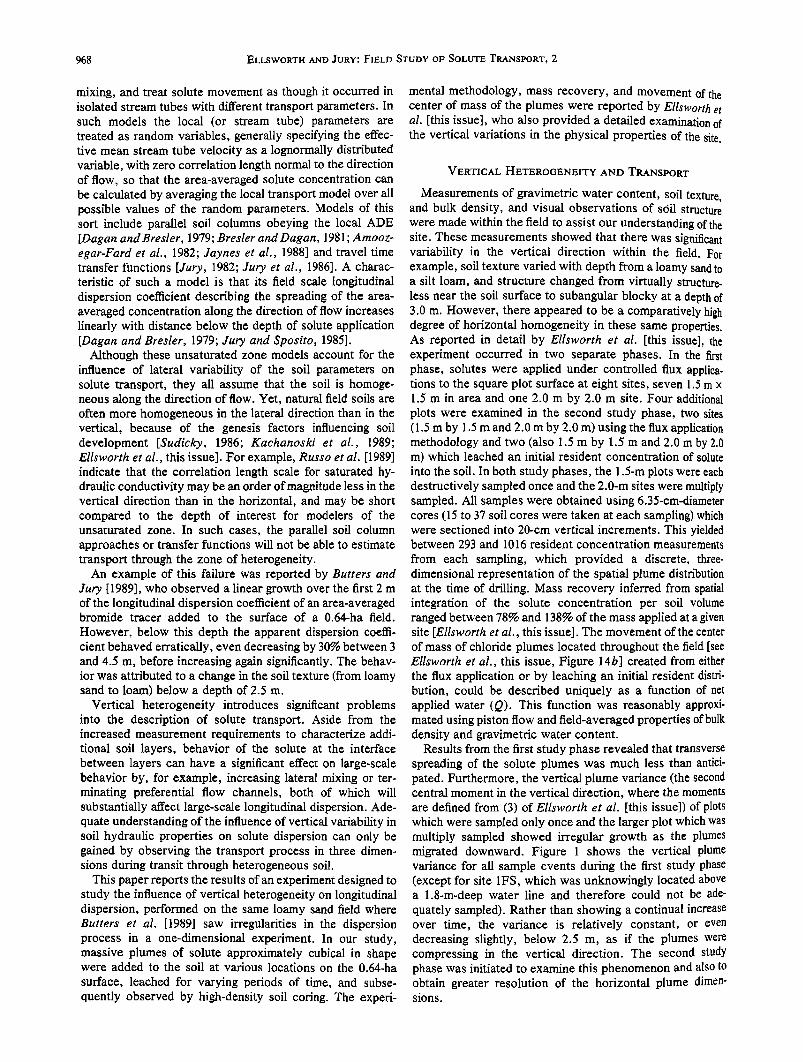
Results from the first study phase revealed that transverse spreading of the solute plumes was much less than antici- pated. Furthermore, the vertical plume variance (the second central moment in the vertical direction, where the moments are defined from (3) of Ellsworth et al. [this issue]) of plots which were sampled only once and the larger plot which was multiply sampled showed irregular growth as the plumes migrated downward. Figure 1 shows the vertical plume variance for all sample events during the first study phase (except for site 1FS, which was unknowingly located above a !.8-m-deep water line and therefore could not be ade- quately sampled). Rather than showing a continual increase over time, the variance is relatively constant, or even decreasing slightly, below 2.5 m, as if the plumes were compressing in the vertical direction. The second study phase was initiated to examine this phenomenon and also to obtain greater resolution of the horizontal plume dimen- sions.
ELLSWORTH AND JURY' FIELD STUDY OF SOLUTE TRANSPORT. 969
6000
< 5O00
0
04000
3000
w 20o0
lOOO
STUDY PHASE 1, FLUX APPLICATION
0 ' 160 260 360 4(•0 DEPTH (CM)
Fig. 1. Vertical plume variance, as a function of net applied water. Data from the first study phase.
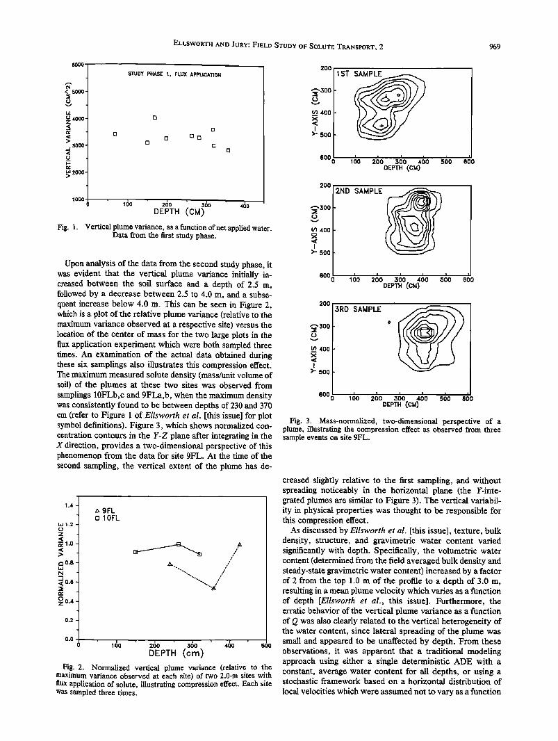
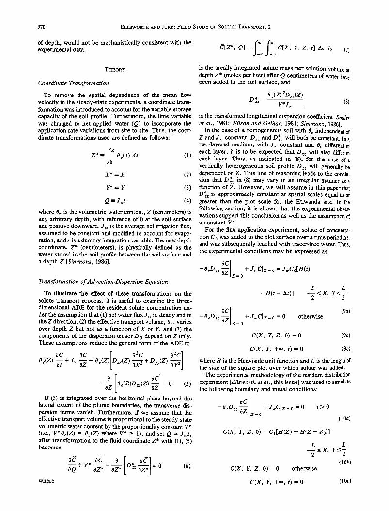
Upon analysis of the data from the second study phase, it was evident that the vertical plume variance initially in- creased between the soil surface and a depth of 2.5 m, followed by a decrease between 2.5 to 4.0 m, and a subse- quent increase below 4.0 m. This can be seen in Figure 2, which is a plot of the relative plume variance (relative to the maximum variance observed at a respective site) versus the location of the center of mass for the two large plots in the flux application experiment which were both sampled three times. An examination of the actual data obtained during these six samplings also illustrates this compression effect. The maximum measured solute density (mass/unit volume of soil) of the plumes at these two sites was observed from samplings 10FLb,c and 9FLa,b, when the maximum density was consistently found to be between depths of 230 and 370 cm (refer to Figure 1 of Ellsworth et al. [this issue] for plot symbol definitions). Figure 3, which shows normalized con- centration contours in the Y-Z plane after integrating in the X direction, provides a two-dimensional perspective of this phenomenon from the data for site 9FL. At the time of the second sampling, the vertical extent of the plume has de-
1.4
1.2
0.8
.<0.6
0.4.
0.2
0.0
zx 9FL [] 10FL
' I' I '"1 0 ' 160 ' 260 ' 360 400 500
DEPTH (cm) Fig. 2. Normalized vertical plume variance (relative to the
maximum variance observed at each site) of two 2.0-m sites with flux application of solute, illustrating compression effect. Each site was sampled three times.
200
•,•oo to
tn 400 x
I >' 500
600
1 ST SAMPLE
0 i•O 21•0 '1 3(•0 •60 51•0' 6•0 DEPTH (CM)
200
•'300
m 400 x
I >-' 500
600 0
2ND SAMPLE
ot•,'r. (cu)
200
•'300 to
(,n 400 x
I >- 500 -
600 0
3ro sAMPLE
166 '" 260 •{•0 •60 560 II $•0 DEPTH
Fig. 3. Mass-normalized, two-dimensional perspective of a plume, illustrating the compression effect as observed from three sample events on site 9FL.
creased slightly relative to the first sampling, and without spreading noticeably in the horizontal plane (the Y-inte- grated plumes are similar to Figure 3). The vertical variabil- ity in physical properties was thought to be responsible for this compression effect.
As discussed by Ellsworth et al. [this issue], texture, bulk density, structure, and gravimetric water content varied significantly with depth. Specifically, the volumetric water content (determined from the field averaged bulk density and steady-state gravimetric water content) increased by a factor of 2 from the top 1.0 m of the profile to a depth of 3.0 m, resulting in a mean plume velocity which varies as a function of depth [Ellsworth et al., this issue]. Furthermore, the erratic behavior of the vertical plume variance as a function of Q was also clearly related to the vertical heterogeneity of the water content, since lateral spreading of the plume was small and appeared to be unaffected by depth. From these observations, it was apparent that a traditional modeling approach using either a single deterministic ADE with a constant, average water content for all depths, or using a stochastic framework based on a horizontal distribution of
local velocities which were assumed not to vary as a function
970 ELLSWORTH AND JURY: FIELD STUDY OF SOLUTE TRANSPORT, 2
of depth, would not be mechanistically consistent with the experimental data. tj[Z*, Q]=•_•oof_•ooC[X, Y,Z,t]dxdy (7)
THEORY
Coordinate Transformation
To remove the spatial dependence of the mean flow velocity in the steady-state experiments, a coordinate trans- formation was introduced to account for the variable storage capacity of the soil profile. Furthermore, the time variable was changed to net applied water (Q) to incorporate the application rate variations from site to site. Thus, the coor- dinate transformations used are defined as follows:
z* -= o as ( )
X* -- X (2)
Y* • Y (3)
Q-=Jwt (4)
where 0• is the volumetric water content, Z (centimeters) is any arbitrary depth, with reference of 0 at the soil surface and positive downward, Jw is the average net irrigation flux, assumed to be constant and modified to account for evapo- ration, and s is a dummy integration variable. The new depth coordinate, Z* (centimeters), is physically defined as the water stored in the soil profile between the soil surface and a depth Z [Simmons, 1986].
Transformation of Advection-Dispersion Equation
To illustrate the effect of these transformations on the
solute transport process, it is useful to examine the three- dimensional ADE for the resident solute concentration un-
der the assumption that (1) net water flux Jw is steady and in the Z direction, (2) the effective transport volume, 0e, varies over depth Z but not as a function of X or Y, and (3) the components of the dispersion tensor D ij depend on Z only. These assumptions reduce the general form of the ADE to
OC OC [ 02C 0 2C 1 o(z) + o + o.(z)
o oc] 0 e(Z)Dzz(Z) = 0 (5) oz
If (5) is integrated over the horizontal plane beyond the lateral extent of the plume boundaries, the transverse dis- persion terms vanish. Furthermore, if we assume that the effective transport volume is proportional to the steady-state volumetric water content by the proportionality constant V* (i.e., V* O,(Z) -- O•(Z) where V* >- 1), and set Q = Jwt, after transformation to the fluid coordinate Z* with (1), (5) becomes
oC aC o o• • + V* D z*z = 0 (6) oQ oZ* oZ*
is the areally integrated solute mass per solution volume at depth Z* (moles per liter) after Q centimeters of water have been added to the soil surface, and
0 v(Z) 2D zz(Z) D* -
zz - V*Jw . (8)
is the transformed longitudinal dispersion coefficient [Smiles et al., 1981; Wilson and Gelhar, 1981; Simmons, 1986].
In the case of a homogeneous soil with Or, independent of Z and Jw constant, Dzz and D* will both be constant. In a two-layered medium, with Jw constant and Or, different in each layer, it is to be expected that D zz will also differ in each layer. Thus, as indicated in (8), for the case of a vertically heterogeneous soil profile D zz will generally be dependent on Z. This line of reasoning leads to the conclu- sion that D}z in (8) may vary in an irregular manner as a function of Z. However, we will assume in this paper that D* is approximately constant at spatial scales equal to or zz
greater than the plot scale for the Etiwanda site. In the following section, it is shown that the experimental obser- vations support this conclusion as well as the assumption of a constant V*.
For the flux application experiment, solute of concentra- tion Co was added to the plot surface over a time period At, and was subsequently leached with tracer-free water. Thus, the experimental conditions may be expressed as
oc
-o eDzz • Z--O
+ J•Clz = o = JwCo[H(t)
L L - H(t- At)] --<X, Y<-
2 2
oc
-o eDzz • Z=0
+ J•Clz = 0 - 0 otherwise (9a)
C(X, Y, Z, O) = 0 (9b)
C(X, Y, +o•, t)= 0 (9c)
where H is the Heaviside unit function and L is the length of the side of the square plot over which solute was added.
The experimental methodology of the resident distribution experiment [Ellsworth et al., this issue] was used to simulate the following boundary and initial conditions:
oc
-o eDzz • Z=0
+ JwClz = o = 0 t > 0
(10a)
C(X, Y, Z, O) = Cl[H(Z) - H(Z- Z0)]
c(x, r, z, o)= o
L L ---<X, Y<-
2 2
(lOb) otherwise
where C(X, Y, +oo, t)= 0 (10c)

ELLSWORTH AND JURY: FIELD STUDY OF SOLUTE TRANSPORT, 2
TABLE 1. Summary of Net Applied Water, Effective Drainage, and Estimated Depth of the Plume Center of Mass in Both Real Space and Transformed Space
Sample NA W Q Qo t a * d NA w Z crn Z •rn .
Flux Experiment 2FS 20.6 25.5 20.6 0.4 68 13.2 3FS 62.7 67.6 18.0 0.4 317 69.4 4FS 40.7 45.5 18.7 0.4 198 40.9 5FS 61.0 66.0 18.4 0.5 282 60.7 6FS 35.0 39.9 18.7 0.4 169 31.7 8FS 49.6 55.1 19.2 1.0 223 43.6 11FS 82.3 87.3 18.8 0.5 357 82.2 9FLa 43.4 49.7 25.6 1.8 238 47.6 9FLb 75.9 82.4 25.6 2.1 356 78.4 9FLc 96.0 107.6 25.6 7.2 427 96.1 10FLa 30.9 35.8 25.6 0.4 150 25.2 10FLb 54.6 60.9 25.6 1.8 263 49.9 10FLc 70.8 76.5 25.6 1.2 319 64.7
Resident Distribution Experiment 7RS 48.0 50.7 0.0 2.7 272 52.8 12RLa 38.2 40.4 0.0 2.2 239 46.4 12RLb 89.6 102.7 0.0 7.2 532 129.7
All units are in centimeters, NA W is the net applied water at the time of sampling, Q and Q0 are as defined in (13) of the text, td*ClNA W is an estimate of the net drainage flux between the last irrigation and the time of sampling, Zcm is the estimated depth of the plume center of mass at the time of .
sampling, and Zero is the corresponding depth in the fluid coordinate system.
971
with Z 0 the depth of incorporation and L and H as defined previously.
After transformation, the boundary and initial conditions appropriate for the flux experiment are given by (11), where Q = Q0 att = At:
-D•z 0-•+ V*•=V*CoL2[H(Q)-H(Q-Qo)] (11a)
Z*=0
O[z*, 0] = o
½[oo, Q] = 0
The appropriate transformed boundary and initial condi- tions for the resident distribution experiment are expressed by
OC
-D h O--• + V* C = 0 Z* = O' Q > 0 (12a)
C[Z*, 0] = L2Ci[H(Z *) - H(Z* - Z•)] (12b)
C[oo, Q] = 0 (12c)
where Z% is the depth of incorporation in the fluid coordinate system.
Equation (6) will be analyzed subject to the experimental conditions defined by (11) and (12), assuming D* is con- zz
stant.
0 Q=NAW+ tadNA w+ W O(s) ds (13a)
Qo TM NAWo (13b)
where the terms on the right-hand side of (13) are defined by Ellsworth et al. [this issue]. Table ! contains, for each sample event in both experiments, NA W, Q, Qo, tadNAw, and the depth of the plume center of mass (estimated from the moment analysis) in both the real space and fluid coordinate system.
In Appendix A, derivations for the zeroth, first, and second "spatial" moments of a plume obeying (6) and (11) (flux application experiment) or a plum. e obeying (6) and (12) (resident distribution experiment) are generated by multiply- ing each side of (6) by Z* •v and integrating from zero to oo and solving the resulting set of ordinary differential equa- tions for the moments subject to the appropriate boundary and initial conditions. From these expressions for the spatial moments, the mean and variance of a solute plume obeying (6) with D* constant and subject to either (11) or (12) can be given as a function of Q for all times after which the resident solute concentration at the soil surface is negligible (Q > Qf, where Qf is the volume of NA W after which the solute concentration at the soil surface is zero). These derivations, for both the flux and resident distribution experiments, result in the following expressions for the plume mean and vari- ance:
PARAMETER ESTIMATION
As explained by Ellsworth et al. [this issue], the water application method (drip emitters or sprinkle irrigation) and the time delay between irrigation and sampling were shown to influence the movement of the plumes' center of mass. Therefore, based on (7) of Ellsworth et al. [this issue], Q for each sample event was computed using
Flux application experiment
Mean (Q)= V*(Q-•-•-Q) + . .. (14a) V*
(-7) ( V * A Q ) 2 + 2 D z* z Q- -3 •-•-•-] Var (Q) ..... 12 (14b)
972 ELLSWORTH AND JURY: FIELD STUDY OF SOLUTE TRANSPORT, 2
120 -
r,.) 100
80.
0 60-
Z 40
2O
FLUX EXPERIMENT CENTER OF MASS VS. 0-0ø/2
(iN FLUID COO
• Y = 1.01-X + 3.71
..... [ J " [ "' I" ' [" I ! I "[ '"l ................ ! ....... I ........ 0 20 40 60 80 1 O0 120
NET APPLIED WATER (CM)
500
450
400
ß -", 350 0
N 300 v
• 250 I 200'
<:Dr
. •= 150' N,• !00'
•. 5o,
o
[]
[] [] [] • Y = 3.21-X R 2 = 0.72
i , , i
o •o ,,o •o •'o ' •o ' •.o•- MEAN DISPLACEMENT (cm)
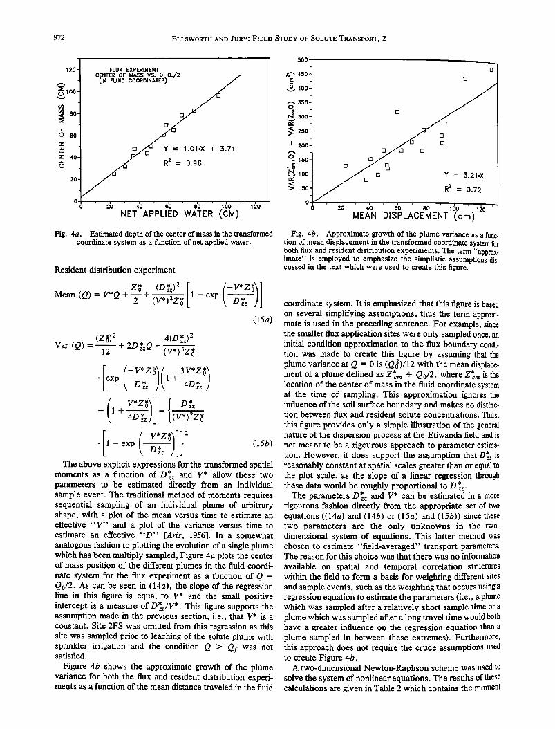
Fig. 4a. Estimated depth of the center of mass in the transformed coordinate system as a function of net applied water.
Resident distribution experiment
Z$ (D•z) 2 Mean (Q)= V*Q +--+
2 (v*)2Z3 1-exp•, D;z / (15a)
(g•) 2 4(D z'z) 2 Vat' ( Q ) = • + 2 D z*z Q +
12 (V*) 3Z•
. ) ( _{ - + (v*)2z
....
Dh The above explicit expressions for the transformed spati•
moments as a function of D* •d V* allow these two parameters to be estimated directly from an individu• sample event. The traditional method of moments requires sequential sampling of an individual plume of arbitrary shape, with a plot of the mean versus time to estimate an effective "V •' and a plot of the v•ance versus time to estimate an effective "D" [Aris, 1956]. In a somewhat analogous fashion to plotting the evolution of a single plume which has been mukiply sampled, Figure 4a plots the center of mass position of the different plumes in the fluid coordi- nate system for the flux experiment as a •nction of Q - Qo/2. As can be seen in (14a), the slope of the regression line in this figure is equal to V* and the small positive intercept is a measure of D•z/V*. This figure suppo•s the assumptio• made in the previous section, i.e., that V* is a constant. Site 2FS was omitted from this regression as this site was sampled prior to leaching of the solute plume with sprinkler i•gation and the condition Q > Qf was not satisfied.
Figure 4b shows the approximate growth of the plume variance for both the flux and resident distribution experi- ments as a function of the mean distance traveled in the fluid
Fig. 4b. Approximate growth of the plume variance as a rune. tion of mean displacement in the transformed coordinate system for both flux and resident distribution experiments. The term "approx. imate" is employed to emphasize the simplistic assumptions dis- cussed in the text which were used to create this figure.
coordinate system. It is emphasized that this figure is based on several simplifying assumptions; thus the term approxi- mate is used in the preceding sentence. For example, since the smaller flux application sites were only sampled once, an initial condition approximation to the flux boundary condi- tion was made to create this figure by assuming that the plume variance at Q = 0 is (Q02)/12 with the mean displace- ment of a plume defined as Z c,• + Q o/2, where * Z cm is the location of the center of mass in the fluid coordinate system at the time of sampling. This approximation ignores the influence of the soil surface boundary and makes no distinc- tion between flux and resident solute concentrations. Thus, this figure provides only a simple illustration of the general nature of the dispersion process at the Eftwanda field and is not meant to be a rigourous approach to parameter estima- tion. However, it does support the assumption that D}z is reasonably constant at spatial scales greater than or equal to the plot scale, as the slope of a linear regression through these data would be roughly proportional to D•z.
The parameters D* and V* zz can be estimated in a more rigourous fashion directly from the appropriate set of two equations ((14a) and (14b) or (lSa) and (15b)) since these two parameters are the only unknowns in the two- dimensional system of equations. This latter method was chosen to estimate "field-averaged" transport parameters. The reason for this choice was that there was no information
available on spatial and temporal correlation structures within the field to form a basis for weighting different sites and sample events, such as the weighting that occurs using a regression equation to estimate the parameters (i.e., a plume which was sampled after a relatively short sample time or a plume which was sampled after a long travel time would both have a greater influence on the regression equation than a plume sampled in between l•hese extremes). Furthermore, this approach does not require the crude assumptions used to create Figure 4b.
A two-dimensional Newton-Raphson scheme was used to solve the system of nonlinear equations. The results of these calculations are given in Table 2 which contains the moment
ELLSWORTH AND JURY: FIELD STUDY OF SOLUTE TRANSPORT, 2 973
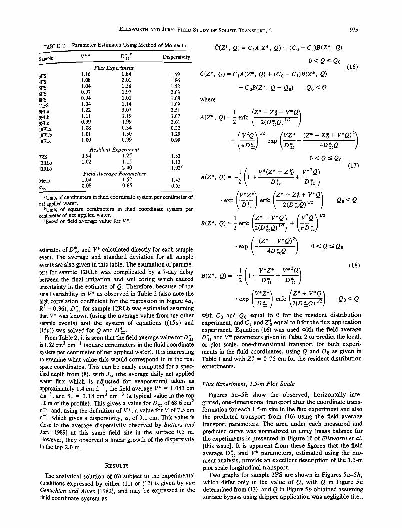
TABLE 2. Parameter Estimates Using Method of Moments • V* a b Sample D •z Dispersivity
Flux Experiment
3FS 1.16 1.84 1.59 4FS 1.08 2.01 1.86 5F$ 1.04 1.58 1.52 6FS 0.97 1.97 2.03 8F$ 0.94 1.01 1.08 11F$ 1.04 1.14 1.09 9FLa 1.22 3.07 2.51 9FLb 1.11 1.19 1.07 9FLc 0.99 1.99 2.01 10FLa 1.08 0.34 0.32 10FLb 1.01 1.30 1.29 10FLc 1.00 0.99 0.99
Resident Experiment 7RS 0.94 1.25 1.33 I2RLa 1.02 1.15 1.13 12RLa 2.00 1.92 c
Field Average Parameters Mean 1.04 1.52 1.45 fin-1 0.08 0.65 0.55
aUNts of centimeters in fluid coordinate system per centimeter of net applied water.
bUnits of square centimeters in fluid coordinate system per centimeter of net applied water.
CBased on field average value for V*.
estimates of D* and V* calculated directly for each sample event. The average and standard deviation for all sample events are also given in this table. The estimation of parame- ters for sample 12RLb was complicated by a 7-day delay between the final irrigation and soil coring which caused uncertainty in the estimate of Q. Therefore, because of the small variability in V* as observed in Table 2 (also note the high correlation coefficient for the regression in Figure 4a, R 2 = 0.96), D*zz for sample 12RLb was estimated assuming that V* was known (using the average value from the other sample events) and the system of equations ((15a) and (15b)) was solved for Q and D•z.
From Table 2, it is seen that the field average value for D* is 1.52 cm 2 cm -1 (square centimeters in the fluid coordinate system per centimeter of net applied water). It is interesting to examine what value this would correspond to in the real space coordinates. This can be easily computed for a spec- ified depth from (8), with Jw (the average daily net applied water flux which is adjusted for evaporation) taken as approximately 1.4 cm d -• , the field average V* = 1.043 cm cm -1, and 0•, = 0.18 cm 3 cm -3 (a typical value in the top 1.0 m of the profile). This gives a value for Dzz of 68.6 cm2 d -1, and, using the definition of V*, a value for V of 7.5 cm d -1, which gives a dispersivity, a, of 9.1 cm. This value is close to the average dispersivity observed by Butters and Jury [1989] at this same field site in the surface 0.5 m. However, they observed a linear growth of the dispersivity in the top 2.0 m.
RESULTS
The analytical solution of (6) subject to the experimental conditions expressed by either (11) or (12) is given by van Genuchten and Alves [1982], and may be expressed in the fluid coordinate system as
C(Z*, Q)= C lA(Z*, Q)+ (Co- C l)B(Z*, Q)
O< Q<- Qo
C(Z*, Q)= ClA(Z*, Q) + (Co- C•)B(Z*, Q) (16)
- CoB( Z* , Q - Q0)
where
Qo<Q
(z* + Z• + V'Q)2.) O< Q< Qo
,
Dzz / 1 ( V* (Z* + Z •) A(Z* Q)=-• 1 + + ' D*
(-z, 1 ß exp Ix D z*z / erfc • •-/•• 1/2 1 [Z*-V*Q• (V2Q• m Q)= .;- +
( (z*- ) -exp - 4D•zQ 0<Q•Q0
(17)
Qo<Q
B(Z*, Q)=-• 1 + D•'---•+ Dz = /
(V'Z* I {Z* + V*Q i -exp D• z ] effc ----•--172'
(18)
Qo<Q
with Co and Q0 equal to 0 for the resident distribution experiment, and C • and Z• equal to 0 for the flux application experiment. Equation (16) was used with the field average D•z and V* parameters given in Table 2 to predict the local, or plot scale, one-dimensional transport for both experi- ments in the fluid coordinates, using Q and Qo as given in Table 1 and with Z% = 0.75 cm for the resident distribution experiments.
Flux Experiment, 1.5-m Plot Scale
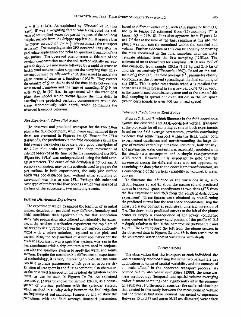
Figures 5a-5h show the observed, horizontally inte- grated, one-dimensional transport after the coordinate trans- formation for each 1.5-m site in the flux experiment and also the predicted transport from (16) using the field average transport parameters. The area under each measured and predicted curve was normalized to unity (mass balance for the experiments is presented in Figure 10 of Ellsworth et al. [this issue]. It is apparent from these figures that the field average D* and V* parameters estimated using the mo- ment analysis, provide an excellent description of the 1.5-m plot scale longitudinal transport.
Two graphs for sample 2FS are shown in Figures 5a-5h, which differ only in the value of Q, with Q in Figure 5a determined from (13), and Q in Figure 5b obtained assuming surface bypass using dripper application was negligible (i.e.,

974 ELLSWORTH AND JURY: FIELD STUDY OF SOLUTE TRANSPORT, 2
Fig. 5. Observed and predicted transport, after transformation, on 1.5-m plots with plumes created from flux application of solute. Predictions based on field average parameters. Figure 5 b shows the prediction without the bypass assumption.
ELLSWORTH AND JURY: FIELD STUDY OF SOLUTE TRANSPORT, 2 975
W = 0 in (13a)). As explained by Ellsworth et al. [this issue], W was a weighting factor which corrected the esti- mate of net applied water for partial bypass of the soil near the plot surface from the dripper application. It appears that the bypass assumption (W = •) overestimates the transport at this site. The sampling at site 2FS occurred 1 day after the final solute application and prior to sprinkler irrigation of the plot surface. The observed phenomenon at this site of the resident concentration near the soil surface initially increas- ing with depth to a maximum followed by a rapid decrease to background concentration supports the sampling time delay assumption used by Ellsworth et al. [this issue] to model the plume center of mass as a function of NA W. They correct the estimate of Q on the basis of the time delay between the most recent irrigation and the time of sampling. If Q is set equal to Q0 in (10) (i.e., in agreement with the traditional piston flow model which would ignore the time delay in sampling) the predicted resident concentration would de- crease monotonically with depth, which contradicts the observed transport behavior.
Flux Experiment, 2.0-m Plot Scale
The observed and predicted transport for the two 2.0-m plots in the flux experiment, which were each sampled three times, are presented in Figures 6a-6f. Except for 9FLa (Figure 6b), the predictions in the fluid coordinates using the field average parameters provide a very good description of the 2.0-m plot scale transport. The deep movement of chloride observed at the time of the first sampling of site 9FL (Figure 6b, 9FLa) was underpredicted using the field aver- age parameters. The cause of this deviation is not certain. A possible explanation may be the methods used to prepare the plot surface. In both experiments, the only plot surface which was not disturbed (i.e., without either rototilling or excavation) was that at site 9FL. Perhaps this enhanced some type of preferential flow process which was masked at the time of the subsequent two sampling events.
Resident Distribution Experiment
The experiment which examined the leaching of an initial resident distribution provided very different boundary and initial conditions than applicable to the flux application study. Site preparation also differed considerably; for exam- ple, in the resident distribution experiment the top 5 cm of soil was physically removed from the plot surface, uniformly mixed with a solute solution, replaced to the plot, and packed. Also, the only method of water application for the resident experiment was a sprinkler system, whereas in the ttux experiment trickle drip emitters were used in conjunc- tion with the sprinkler system to apply the water and solute solution. Despite the considerable differences in experimen- tal methodology, it is very interesting to note that the same two field average parameters which gave an accurate de- scription of transport in the flux experiment also character- ize the observed transport in the resident distribution exper- iment, as can be seen in Figures 7a-7d. As explained previously, Q was unknown for sample 12RLb, as a conse- quence of physical problems with the sprinkler system, which resulted in a 7-day delay between the final irrigation and beginning of soil sampling. Figures 7c and 7d show the predictions with the field average transport parameters
based on different values of Q, with Q in Figure 7c from (13) and Q in Figure 7d estimated from (15) assuming V* is known (Q = 119.18). It is also apparent from Figures 7c and 7d that at the time of the final sampling at this site, the plume was not entirely contained within the sampled soil volume. Further evidence of this can be seen by comparing the mass recovered in this final sampling with the mass estimate obtained from the first sampling (12RLa). The estimate of mass recovered for sampling 12RLb was 75% of that computed from sample 12RLa (1.52 kg and 2.10 kg of chloride, respectively [Ellsworth, 1989]). Based on the esti- mate of Q from (15), the field average D* parameter closely zz
approximates the observed spreading at the final sampling of site 12RL. This is quite remarkable when it is recalled that solute was initially present in a narrow band of 0.75 cm width in the transformed coordinate system and at the time of this final sampling is spread out over 100 cm in the Z* space (which corresponds to over 400 cm in real space).
Transport Predictions in Real Space
Figures 5, 6, and 7, which illustrate in the fluid coordinate system the observed and ADE-predicted vertical transport at the plot scale for all sampling events in both experiments based on the field average parameters, provide convincing evidence that solute transport within the field, under both experimental conditions and notwithstanding the large de- gree of vertical variability in texture, structure, bulk density, and gravimetric water content, was reasonably modeled with the steady-state assumption and a simple two-parameter ADE model. However, it is important to note that the agreement among the different sites was not apparent by examining the data prior to the coordinate transformation, as a consequence of the vertical variability in volumetric water content.
To illustrate the influence of the variations in 0v with depth, Figures 8a and 8b show the measured and predicted curves in the real space coordinates at two sites (4FS from the flux experiment and 7RS from the resident distribution experiment). These figures were obtained by transforming the predicted curves into the real space coordinates using the measured water content at each site (numerical inversion of (1)). The skew in the predicted curves to the left of the plume center is simply a consequence of the lower volumetric water content in the loamy sand portion of the profile (0-2.5 m depth) relative to that in the loam texture (between 2.5 and 4.0 m). The skew toward the left from the plume centers in the observed data in Figures 8a and 8b is thus attributed to the volumetric water content variations with depth.
CONCLUSIONS
The observation that the transport at each individual site was reasonably modeled using the same two parameters has implications in terms of spatial variability and the concept of a "scale effect" in the observed transport process. As pointed out by Moltyaner and Killey [1988], the measure- ment methodology (temporal and spatial volume averaging and/or discrete sampling) can significantly alter the parame- ter estimates. Furthermore, consider the scale relationships that existed in this study between the measurement volume and the process that measurement was meant to represent. Between 15 and 37 soil cores (6.35 cm diameter) were taken

976 ELLSWORTH AND JURY: FIELD STUDY OF SOLUTE TRANSPORT, 2
.......... sd•p, r •o•
•' '• --?•--•e• d• •o (•c•u TRANSFORMED DEPTH COORDINATE )
b
D D ,
13000 , Onn
m•qsronuœn orrin COOnmNATœ (CU)
c SAMP• 10FLb
o u [A.1Ul•
-- PREDIC!•
• •1• 8•g 7• 11• --=-= 1• 11• TRAN$?ORU[D DœPTH COORDINATE (CU)
d SAIdP• r' gF'Lb
o W[J•,Ul!tO
-- IHI[OCT-•
- _
• •l 7t3 l&0 1• 11• TRANSFORIMœD DœPTH COORDINATE:
IQ
e z SAWPLE 10FLe
(cu)
•PLE gFLg
13 w r. ASuIIn•
-- PRI:DCTTD
0
,lj5-- I• 7• I&D 1• TRAJqSF'ORWED DEJ:rr'H COORDINATE
Fig. 6. Observed and predicted transport, after transformation, on 2.0-m flux application sites, where each site was sampled three times. Predictions based on field average parameters.
at each sample event, of which a subset, perhaps 10, were located within the borders of a plot. From these general estimates, it is easily determined that the percent of a 2.0-m plot surface represented by the cross-sectional area of these cores was less than 1%, and further, that this scale of measurement characterized much of the "field scale" vari-
ability (where field scale refers to the spatial domain repre- sented by the 11 individual sites studied in both experimental phases). The latter conclusion follows from the observation that the same two parameters reasonably modeled the ob- served transport at each site.
The transformation given by (1)-(4) provided a means of "scaling" the observed transport phenomena, in both the horizontal and vertical directions, through elimination of the influence of large-scale (i.e., greater than plot scale) horizon- tal variability in water content and reduction of the deter- ministic influence of the vertical variations in volumetric water content at a specific site. Because of the intense sampling procedures used in the study, about 20 samples per each 20 cm depth increment were taken with every sampling event. The large number of measurements taken, coupled with the low observed variance in gravimetric water content

ELLSWORTH AND JURY: FIELD STUDY OF SOLUTE TRANSPORT, 2 977
a • I .......... SA•,r •2:•L. 13 iID•.IURE:D
-- PR[D•
"---• .b •b--•o •b •b •h TRANSFORUED DEPTH COORDINATE (Cid)
21 o
b ' SXUPL[ 7•s
[3 ¾r..kSUREO
-- PR[DICTED
TRANSFOR!dœD DEPTH COORDINATE CCM)
[3 MrJ•suRrh
-- PII•DICIT. D
TRANSFORMED DEPTH COORDINATE
d IdEASURE/)
PI•DICTED
O
TRAHSFORUED DEPTH COORDINATE
Fig. 7. Observed and predicted transport, after transformation, with plume initially present in a 5-cm narrow band at the plot surface. Figure 7c was obtained using Q from (13) and Figure 7d with Q estimated from (15), assuming V* is known. Predictions based on field average parameters.
at a specific site and depth, provided assurance that mea- surement errors in the transformation were minimal.
It is also interesting to observe that despite the variations in structure and texture with depth, the transformed data were reasonably modeled in both the loamy sand and loam texture regions with the same two parameters. After the transformation, it is not unreasonable to expect that V* would be approximately constant with depth. The regression
of the center of mass in the Z* space versus Q - Qo/2 (Figure 4a) suggested this was the case. The observation that the average V* was greater than 1 further indicated the existence of a small volume of the wetted pore space which did not appear to contribute to solute transport. This ex- cluded volume was reasonably constant with depth despite the increase in clay and silt. However, prior to analysis, it was not expected that the quantity in (8), D}z, could be
a o SAuP•r ,kr'S .......
• L• 001•r•n,-,,-,r• .... D[PTH
b .•AkJPLE 7RS
- PR[DICTED
DEPTH
Fig. 8. Real space observed and predicted transport, with prediction made in transform space and numerically inverted using measured volumetric water content distribution. The observed skew to the left of the plume center is a consequence of vertical variations in volumetric water content.
978 ELLSWORTH AND JURY: FIELD STUDY OF SOLUTE TRANSPORT, 2
modeled as approximately constant over the depth of trans- port. The fact that this was the case in the present study is quite interesting and merits future research.
The observations from this work, obviously specific to this site and experimental conditions, suggest that a laboratory experiment performed on an "undisturbed" soil column (which was large enough to characterize the variability represented in the soil cores taken at each sampling event) could be used to predict most of the field scale solute transport, if combined with field measurements of evapora- tion and volumetric water content.
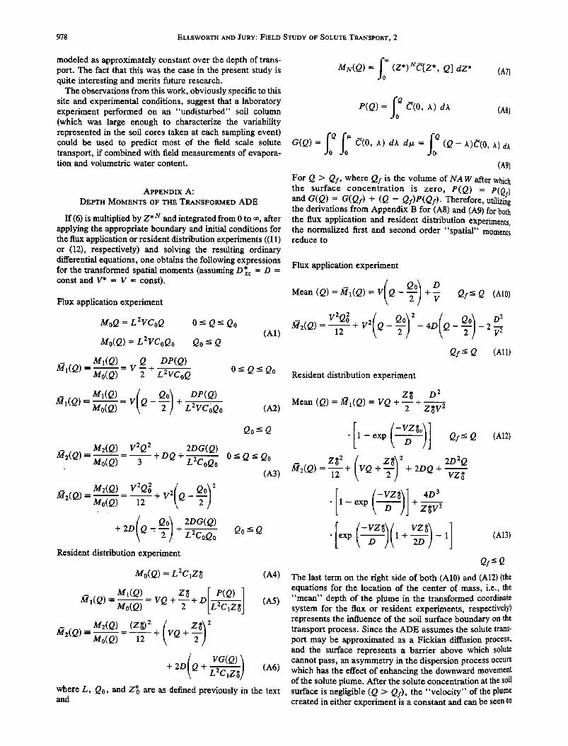
APPENDIX A:
DEPTH MOMENTS OF THE TRANSFORMED ADE
If (6) is multiplied by Z* N and integrated from 0 to •, after applying the appropriate boundary and initial conditions for the flux application or resident distribution experiments ((11) or (12), respectively) and solving the resulting ordinary differential equations, one obtains the following expressions for the transformed spatial moments (assuming D* = D = const and V* = V = const).
Flux application experiment
MoQ = L 2VCoQ 0 < Q-< Qo
Mo(Q) = L2VCoQo Qo '< Q (A1)
Ml(Q) Q DP(Q)
Mi(Q) Mo(Q) V • + L ZVCoQ O_< Q<_Qo
M•(Q)(_•)DP(Q) IOI(Q) = Mo(Q) = v Q - + L2VC•Qo (A2)
M2(Q) V2Q 2 2DG(Q) M2(Q) Mo(Q) 3 •- DQ + • L2CoQo
3•2(Q) m Mo(Q) = 1"•-- + V2 Q -
Qo) 2DG(Q) + 2D Q--•- +L2CoQ-•- • Resident distribution experiment
Qo-< Q
O_<Q< Qo
(A3)
Qo -< Q
Mo(Q) = L 2C1Z •
_ Mi(Q) VQ + + D Mi(Q) -=Mo(Q) -- •'-
- M2(Q)(Z•)2(7 ) M2(Q )mMo(Q) = 1--• + VQ +
P(Q) ] 2
VG(Q) • + 2D Q + L-•I-•]
(A4)
(A5)
(A6)
where L, Q0, and Z• are as defined previously in the text and
MN(Q) = (Z*) NC[Z*, Q] dZ* (A7)
P(Q) =fl 2 •(0, A) dA (AS)
(•9)
For Q > Qf, where Qf is the volume of NA W after which the surface concentration is zero, P(Q) = p(Qf) and G(Q)= G(Qf) + (Q - Qf)P(Qf). Therefore, utilizing the derivations from Appendix B for (A8) and (A9) for both the flux application and resident distribution experiments, the normalized first and second order "spatial" moments reduce to
Flux application experiment
Mean(Q)=3•(Q)=V Q- +- Qf-< Q (A10) V
3•2(Q) = 1-•- + V2 Q - + 4D Q - - 2 V-- •. Qf < Q (All)
Resident distribution experiment
Z• D 2 Mean (Q) = 3•l(Q) = VQ + -- +
2 Z$V 2
M2(Q)= 1• + VQ + + 2DQ + VZ•
[ (-VZ•)] 4D 3 ß 1 - exp D + •V 3 Z
+ 2D ]- (A3) Qi• Q
The last term on the right side of both (A10) and (A12) (the equations for the location of the center of mass, i.e., the "mean" dep• of the plume in the transformed coordinate system for the flux or resident experiments, respectively) represents the influence of the soil surface bound• on the transpo• process. Since the ADE assumes the solute trans- port may be approximated as a Fic•an d•usion process, and the surface represents a ba•er above which solute cannot pass, • asymmetry in the dispersion process occurs which has the effect of enh•cing the downward movement of the solute plume. Mter the solute concentration at the soil surface is negligible (Q > Qf), the "velocity" of the plume created in either experiment is a constant and can be seen to
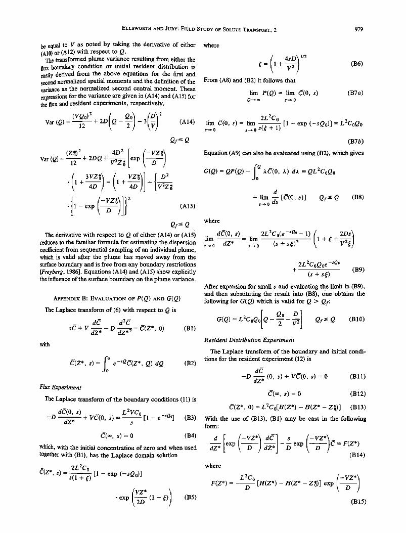
ELLSWORTH AND JURY: FIELD STUDY OF SOLUTE TRANSPORT, 2 979
be equal to V as noted by taking the derivative of either (A10) or (A12) with respect to Q.
The transformed plume variance resulting from either the flux boundary condition or initial resident distribution is easily derived from the above equations for the first and second normalized spatial moments and the definition of the variance as the normalized second central moment. These expressions for the variance are given in (A14) and (A15) for the ttux and resident experiments, respectively.
+2D Q- -3 (A14) 12
Qf<-Q
(zl) 2 Var (Q) = - i2 + 2DQ + V3Z• exp D
3VZ• 1 + - . ß 1 + 4D - 4D] V2Z•
(A15)
Qf-<Q
The derivative with respect to Q of either (A14) or (A15) reduces to the familiar formula for estimating the dispersion coefficient from sequential sampling of an individual plume, which is valid after the plume has moved away from the surface boundary and is free from any boundary restrictions [Freyberg, 1986]. Equations (A14) and (AI$) show explicitly the influence of the surface boundary on the plume variance.
APPENDIX B' EVALUATION OF P(Q) AND G(Q)
The Laplace transform of (6) with respect to Q is
d• d2C
sC + V d'-•- D dZ'. 2 = C(Z*, O) (B1)
with
•(Z*, s)= e-sQC(z *, Q) dQ (B2)
Flux Experiment
The Laplace transform of the boundary conditions (11) is
d•7(O, s) L 2VCo -O + V•(O, s) = • [ 1 - e-seo] (B3)
dZ* s
(7(o0, s) = 0 (B4)
which, with the initial concentration of zero and when used together with (B1), has the Laplace domain solution
2L2C - = 0 [1 - exp (-sQ0)] c(z*, s) + g)
VZ* ) ß exp [2D (1 - •:) (B5)
where
4sD• •:= 1 +-•_ ] From (AS) and (B2) it follows that
1/2
(B6)
lira P(Q)= lim Off(0, s) Q•*: s•0
(B7a)
2L2C0 lira (7(0, s) = lira s-,.o $-,.o s(s c + 1)
[ 1 - exp (-sQ0) ] = LZCoQ 0
(B7b)
Equation (A9) can also be evaluated using (B2), which gives
G(Q) = QP(Q) - fo :2 x •(0, x) dX = QL2CoQ o d
+ lim •ss [C(0, s)] Qf_< Q (B8) s---• 0
where
de(0, s) lira • = lira s-• O dZ* 2L2C0(e-sQø _ 1) ( 2Ds• (s + s•) 2 I + s c + V2e]
2L2CoQo e-sQø + (B9)
(s +
After expansion for small s and evalua[ing the limit in (B9), and then substituting the result into (B8), one obtains the following for G(Q) which is valid for Q > Qf:
G(Q) = L 2CoQo[Q Qo D ] 2 •'2' Qf<Q (B10)
Resident Distribution Experiment
The Laplace transform of the boundary and initial condi- tions for the resident experiment (12) is
dC
-D d'-• (0, s) + VC(0, s) = 0 (B• 1) C(o•, s) = 0 (Bi2)
C'(Z*, O) = L 2Co[H(Z*) - H(Z* - Z•)] (B13)
With the use of (B13), (B1) may be cast in the following form:
dZ* exp -• exp • = F(Z*) (B14)
where
L2Cø [H(Z.) _ H(Z. _ Z}•)] exp (•7* ) F(z*) = - D"'
(B15)

980 ELLSWORTH AND JURY: FIELD STUDY OF SOLUTE TRANSPORT, 2
It is straightforward to solve for the Green's function solu- tion of the Sturm-Liouville operator defined by (B 14) [But- kov, 1968] where Green's function satisfies the equation
d - dG
dZ,
-• exp (J(Z*IA, s) = 8(Z* - A) (B16)
which gives
(z*lx, s)= exp [Z*(1 + s e) + A(1 -
Vs e + I exp (Z*+A)(1-•) 0_<Z* <A
D C(z*lx, s)=
(B17)
exp •-• [A(1 + •) + Z*(1 -
. exp (Z* + X)(1 - s e) + A_<Z*
Thus, the Laplace domain solution which satisfies (B14) is
s)= (z*lx, s)F(X) ax (B18)
where F(X) is given by (B 15). After performing the integra- tion in (B 18) one obtains
_ 2L2CoD { 2s e C(Z*, S)=v2se(s e+ 1) (g-l)
-exp •-•(•+I)(Z*-Z•)
-(s e+ 1) 2 exp L2D (l-f)
ß '(•:_ 1) 2+exp 2D (se +1) (B19)
Equation (B 19) can now be used to evaluate (B7a) and (B8) by setting Z* = 0 and rearranging, which gives
4L2Co D •(0, S)=v2(•:+ 1) 2 1-exp . 2D (s e+l) (B20)
Therefore, for Q > Qf, after which the solute concentration at the soil surface is zero, one finds that
p(Q)= lim •(0 s) L2CoD [ (-VZ•) , V2 1 -exp ß s->0 D (B21)
Q-<Q
lim •(0 s)=lim V4 3 exp (•+1) -1 •--.o as ' •-•o •(s e + 1) •, 2D-
4L2CoZ•yD (-VZ• ) V3---• 7 ii 5 exp [, 20 (se + 1)
2L2CøD2[ (-VZ•)(I + -1 V4 exp D 2D// (B22)
Hence, for the resident distribution experiment, G(Q)is given by
G(Q) = V2 1 - exp D
2L 2CoD 2 V 4 exp D 1 + 2D//- 1 Qf<Q
(B23)
Acknowledgments. The authors would like to thank the Electric Power Research Institute, the Southern California Edison Corn. pany, and the University of California, Riverside, Toxic Substances Research and Training Program for financial assistance on this project.
REFERENCES
Amoozegar-Fard, A., D. R. Nielsen, and A. W. Warrick, Soil solute concentration distributions for spatially varying pore water veloc. ities and apparent diffusion coefficients, Soil Sci. Soc. Am. J., 46, 3-8, 1982.
Aris, R., On the dispersion of a solute in a fluid flowing through a tube, Proc. R. $oc. London, Ser. A, 235, 67-78, 1956.
Biggar, J. W., and D. R. Nielsen, Spatial variability of the leaching characteristics of a field soil, Water Resour. Res., 12, 78-84, 1976.
Bresler, E., and G. Dagan, Convective and pore scale dispersive solute transport in unsaturated heterogenous fields, Water Re- sour. Res., 17, 1683-1693, 1981.
Butkov, E., Mathematical Physics, Addison-Wesley, Reading, Mass., 1968.
Butters, G. L., and W. A. Jury, Field scale transport of bromide in an unsaturated soil, 2, Dispersion modeling, Water Resour. Res., 25, 1583-1598, 1989.
Butters, G. L., W. A. Jury, and F. F. Ernst, Field scale transport of bromide in an unsaturated soft, 1, Experimental methodology and results, Water Resour. Res., 25, 1575-1581, 1989.
Dagan, G., Solute transport in heterogeneous porous formations, J. Fluid Mech., 145, 151-177, 1984.
Dagan, G., and E. Bresler, Solute dispersion in unsaturated heter- ogeneous soil at field scale, I, Theory, Soil Sci. Soc. Am. J., 43, 461-167, 1979.
Domenico, P. A., and G. A. Robbins, A dispersion scale effect in model calibrations and field tracer experiments, J. Hydrol., 70, 123-132, 1984.
Ellsworth, T. R., Field-scale spatial and temporal characterization of solute plume transport through unsaturated porous media, Ph.D. dissertation, Univ. of Calif., Riverside, !989.
Ellsworth, T. R., W. A. Jury, F. F. Ernst, and P. J. Shouse, ^ three-dimensional field study of solute transport through unsatur- ated, layered, porous media, 1, Methodology, mass recovery, and mean transport, Water Resour. Res., this issue.
Freyberg, D. L., A natural gradient experiment in a sand aquifer, 2, Spatial moments and the advection and dispersion of nonreactive tracers, Water Resour. Res., 22, 2031-2046, 1986.
Gelhar, L. W., and C. L. Axness, Three-dimensional stochastic analysis of macrodispersion in aquifers, Water Resour. Res., 19, !61-180, !983.
Gelhar, L. W., A. L. Gutjahr, and R. L. Naff, Stochastic analysis of

ELLSWORTH AND JURY: FIELD STUDY OF SOLUTE TRANSPORT, 2 981
macrodispersion in a stratified aquifer, Water Resour. Res., 15, 1387-1397, 1979.
Gelbar, L. W., A. Mantoglou, C. Welty, and K. R. Rehfeldt, A review of field-scale physical solute transport processes in satu- rated and unsaturated porous media, Top. Rep. EA-4190, Electric Power Res. Inst., Palo Alto, Calif., 1985.
Jaynes, D. B., R. C. Rice, and R. S. Bowman, Independent calibration of a mechanistic-stochastic model for field-scale solute transport under flood irrigation, Soil Sci. Soc. Am. J., 52, 1541- 1546, 1988.
Jury, W. A., Simulation of solute transport using a transfer function model, Water Resour. Res., 18, 363-368, 1982.
Jury, W. A., and G. Sposito, Field calibration and validation of solute transport for the unsaturated zone, Soil Sci. Soc. Am. J., 49, 1331-1341, 1985.
Jury, W. A., G. Sposito, and R. E. White, A transfer function model of solute transport through soil, 1, Fundamental concepts, Water Resout'. Res., 22, 243-247, 1986.
Kachanoski, R. G., I. Van Wesenbeeck, and C. Hamlen, Spatial variability of water and solute flux in a layered soil, in Agronomy Abstracts, p. 187, American Society of Agronomy, Madison, Wis., 1989.
Miller, R. J., Biggar, J. W., and D. R. Nielsen, Chloride displace- ment in Panoche clay loam relation to water movement and distribution, Water Resour. Res., 1, 63-73, 1965.
Moltyaner, G. L., and R. W. D. Killey, Twin Lake tracer tests: Longitudinal dispersion, Water Resour. Res., 24, 1613-1627, 1988.
Nielsen, D. R., and J. W. Biggar, Miscible displacement, III, Theoretical considerations, Soil Sci. Soc. Am. Proc., 26,216-221, 1962.
Pickens, J. F., and G. E. Grisak, Scale-dependent dispersion in a stratified aquifer, Water Resour. Res., 17, 1191-1211, 1981.
Russo, D., W. A. Jury, G. L. Butters, Numerical analysis of solute transport during transient irrigation, 1, The effect of hysteresis and profile heterogeneity, Water Resour. Res., 25, 2109-2118, 1989.
Simmons, C. S., A generalization of one-dimensional solute trans- port: A stochastic-convective flow conceptualization, paper pre- sented at 6th Annual AGU Front Range Branch Hydrology Days, Fort Collins, Colo., April 15-17, 1986.
Smiles, D. E., K. M. Perroux, S. J. Zegelin, and P. A. C. Raats, Hydrodynamic dispersion during constant rate adsorption of water by soil, Soil Sci. Soc. Am. J., 45,453-458, 1981.
Sposito, G., W. A. Jury, and V. K. Gupta, Fundamental problems in the stochastic convection-dispersion model of solute transport in aquifers and field soils, Water Resour. Res., 22, 78-88, !986.
Starr, J. L., H. C. DeRoo, C. R. Frink, and J. Y. Parlange, Leaching characteristics of a layered field soil, Soil Sci. Soc. Am. J., 42, 386-391, 1978.
Sudicky, E. A., A natural gradient experiment on solute transport in a sand aquifer: Spatial variability of hydraulic conductivity and its role in the dispersion process, Water Resour. Res., 22, 2069-2082, 1986.
Sudicky, E. A., J. A. Cherry, and E. O. Frind, Migration of contaminants at a landfill: A case study, 4, A natural-gradient dispersion test, J. Hydrol., 63, 81-108, 1983.
Taylor, G. I., The dispersion of matter in solvent flowing slowly through a tube, Proc. R. Soc. London, Ser. A, 219, 189-203, 1953.
Van de Pol, R. M., P. J. Wierenga, and D. R. Nielsen, Solute movement in a field soil, Soil Sci. Soc. Am. J., 41, 10-13, 1977.
van Genuchten, M. T., and W. J. Alves, Analytical solutions of the one-dimensional convective-dispersive solute transport equation, Tech. Bull. 1661, 151 pp., U.S. Dep. of Agric., Washington, D.C., 1982.
Wartick, A. W., Biggar, J. W., and D. R. Nielsen, Simultaneous solute and water transfer for an unsaturated soil, Water Resour. Res., 7, 1216-1225, 1971.
Wilson, J. L., and L. W. Gelhar, Analysis of longitudinal dispersion in unsaturated flow, 1, The analytical method, Water Resour. Res., 17, 122-130, 1981.
T. R. Ellsworth, Department of Agronomy, University of Illinois at Urbana-Champaign, 1102 South Goodwin Avenue, Urbana, IL 61801.
W. A. Jury, Department of Soil and Environmental Science, University of California, Riverside, CA 92521.
(Received March 21, 1990; revised November 5, 1990; accepted January 15, 1991.)