solute transport in two layered porous media … dqm to solve three one-dimensional aquifer flow...

IOSR Journal of Mechanical and Civil Engineering (IOSR-JMCE)

e-ISSN: 2278-1684,p-ISSN: 2320-334X, Volume 13, Issue 5 Ver. V (Sep. - Oct. 2016), PP 41-52

www.iosrjournals.org

DOI: 10.9790/1684-1305054152 www.iosrjournals.org 41 | Page

Solute Transport In Two Layered Porous Media (Separated

Diagonally) Using Suitable DQM Scheme

Meysam Ghamariadyan1, Seyed Hamed Meraji

2, Abbas Ghaheri

3

1(Civil Eng. Dept. , Iran university of science and technology, Iran)



Abstract: In this research, we presented Differential Quadrature Method for solving groundwater flow and

advection-dispersion equations in two layered porous media which the layers are separated diagonally. This

method was applied to five cases and the results are compared with Modflow and Mt3d solutions. Also, The

effect of various parameters on transport process are discussed in all cases. The DQM results show a good

agreement with Modflow and Mt3d results regarding selecting fewer grid points. In applying the DQM, the

needed mesh size is much smaller than the traditional approaches which reduces computational time and

needed less computer storage capacity.

Keywords: transport, two layer porous media, Differential Quadrature method.

I. Introduction Knowledge of solute transport through composite or layered porous media is of importance to better

manage and describe the movement of solutes in natural and artificial media. Interest in porous media transport

is increasingly motivated by concerns over the presence of a wide variety of contaminant substances and wastes

in the subsurface environment. Porous media are seldom homogeneous and the transport properties of these

media will vary spatially and sometimes also temporally. In some cases artificial barriers are used to prevent or

slow down the progress of certain pollutants. Mathematical models are necessary to describe the fate and

movement of such solutes.

The general framework of the problem can be modeled by a pair of partial differential equations, the

first of which is for the groundwater flow subject to two constant heads and the second is ADE for contaminant

transport. The Advection–diffusion equation describes the solute transport due to the combined effect of

diffusion and convection in a medium. It is a partial differential equation of parabolic type, derived on the

principle of conservation of mass using Fick’s law.

In the past, several investigations have been done to predict the location and movement of the

contaminant. All of them accompanied with some simplicity Assumptions. Analytical solutions for ADE

through semi-infinite or finite porous media have been presented by several researchers (Shamir and Harleman

[1]; Alniami and Rushton [2]). Further researches were done with less simplification. Leij et al. [3] investigated

the solute transfer in layered soil. They utilized two different approaches for solving ADE. Leij and van

Genuchten [4] in their supplementary investigations presented an approximate analytical solution for solute

transport in two-layer porous media with more focus on the interface condition. Recently Li and Cleall [5]

presented analytical solutions for advective and dispersive solute transport in double layered finite porous media

in one-dimension which almost cover all the solutions mentioned by other researchers. In all above researches a

constant flow have been assumed. So, the groundwater flow is not considered in those studies. Also, those

researches have been conducted in one-dimension which cannot perfectly show the solute path and fate in

porous media.

Nowadays, there widely use models for groundwater flow and solute transport, such as MODFLOW

and SUTRA and finding the simplest and optimum techniques to solve the partial differential equation has

attracted a great importance. The frequently used numerical techniques for solving such equations are the

standard finite difference method (FDM), finite element method (FEM) and boundary element method (BEM).

Usually, the FDM requires a large number of points in order to produce a moderately accurate solution while the

rest of the above-mentioned methods are quite sophisticated and involve complex computer programming

algorithms. But there exist a number of alternative methods such as Differential Quadrature Method which can

provide relatively accurate results with inexpensive computation. The DQM has been applied successfully to

solve a wide range of problems, with a diversity of boundary conditions easily and precisely.

DQM first developed by Bellman and Casti [6] and has made a noticeable success over the last four

decades. The main idea of this method is on the basis of the integral quadrature. Further developments achieved

by Shu et al. [7] based on Polynomial-based differential quadrature, (PDQ) (Shu and Richards [8]; Shu et al. [9]

), Fourier expansion-based differential quadrature (FDQ) ( Shu and Xue [10]; Shu and Chew [11]) and RBF-DQ

Solute Transport In Two Layered Porous Media (Separated Diagonally) Using Suitable DQM ..


based on Radial Basis Function, (Shu et al. [12], [13]). Now DQM has been applied successfully in many fields

such as fluid dynamics (Shu et al. [14],[15]; Tsai et al. [16]), solid mechanics (Wang et al. [17]), chemical

engineering (Civan, [18]; Li and Mulay [19]), vibration and buckling (Mahmoud et al. [20]; Danesh et al. [21]),

Geotechnics (Chen et al. [22]), mass transfer (Char et al. [23]). In groundwater fields, Kaya and Arisoy [24]

used DQM to solve three one-dimensional aquifer flow equation problems including a confined aquifer flow

with time dependent boundary conditions, a composite confined aquifer and an unconfined aquifer with

seepage.

Robati and Barani [25] considered water surface profile in an underground canal using DQM model.

They concluded that DQM has the ability to simulate the water surface profile and the results are very close to

the real water surface profile. They compared the DQM results to the results of an analytical and Explicit/

Implicit FDM solutions and obtained a good agreement. In hydraulic and free surface water flow fields, the

work done by Kaya and Arisoy [26] to solve the Saint-Venant equations for linear long wave propagation in

open channels, Kaya et al. [27] to solve a flood propagation problem in open channel can be pointed out. Bert

and Malik [28] have reviewed various papers related to DQM and recited a complete description about

researcher's work at different times. But the application of this method in contaminant transport in porous media

especially in two layered porous media has not been investigated previously.

Due to the inherently complex boundary conditions and intricate physical geometries in any practical

problem, an analytical solution is not possible. This paper presents a DQ method (DQM) for modeling

contaminant transport into two layered aquifer systems. The DQM is used to solve the groundwater flow and

transport equations in a layered confined aquifer The DQM results are verified against Modflow and Mt3d

results.

II. Mathematical Formulation of the Problem Heading s A confined aquifer was assumed which layers are separated diagonally. Each layer has its own specific

characteristics in terms of soil and transport properties. The left and right of the aquifer exposed to a constant

head (1 2 H and H ). Therefore, a steady water flow will be established. Contaminant source is released at the left

boundary of the aquifer system (Fig. 1).

Fig. 1. Problem description of contaminant transport in layered confined aquifer.

As mentioned earlier, the contaminant problem can be described with two equations. The first is a

groundwater flow equation. A two-dimensional equation describing groundwater flow in an confined The

aquifer is given by:

+ =0 xx zz

h hK K

x x z z

(1)

Where "h" is the hydraulic head (L), ,xx zzK K are the permeability ( 1LT ) of aquifer materials in x

and z coordinates, and sS is the specific storage coefficient ( 1L ).

The second equation is the advective–dispersive transport equation (Zheng, 1992) for a reactive solute

in a saturated flow regime showing retardation and decay, such as any loss from irreversible sorption (Baek et

al., 2003) and/or volatilization, can be written as:

( ) .ij i

i j i

C CD C C

t x x x

(2)

Where ix is the sportial coordinate (x, z), R is the retardation factor, C is the solute concentration, ijD is the

hydrodynamic dispersion coefficient tensor (2 1L T

), i is the average linear flow velocity (1LT ) and is the



first-order decay rate coefficient ( 1T ) representing any losses such as volatilization and/or irreversible sorption.

Assuming that molecular diffusion is negligible, the dispersion tensor, may be expressed as: 2 2

*x zxx L TD D

(3)

2 2*z x

zz L TD D

(4)

( ) x zxz zx L HD D

(5)

Where , *D is constant effective diffusion coefficient ( 2 1L T ), L and

T are the longitudinal and

transverse dispersivities (L), respectively, ,x z are the components of the velocity vector, and

2 2 1/2( ) .x z

To obtain a unique solution to (1) and (2), initial and boundary conditions must be specified. In the

flow equation, the initial condition may be expressed as

0( , : 0) ( , ) in Rh x z h x z (6)

The boundary conditions may be stated as follows.

0i

h

n

At the upper and lower boundary (7)

1( , ; ) ( , ; )b bh x z t h x z t At the left boundary (8)

2( , ; ) ( , ; )b bh x z t h x z t At the right boundary (9)

Where in is the outward unit vector normal to the boundary, ( , )b bx z is the spatial coordinate on

the Boundary and 1 2, h h are constant head values.

For the transport equation, the initial condition may be expressed as

0( , : 0) ( , ) at Rb bC x z C x z (10)

The boundary conditions may be stated as follows.

0n

CV

n

At the upper and lower boundary (11)

1 1 1( , ; ) ( , ; )C x z t C x z t At the left (influent) boundary (12)

0C

z

At the right (effluent) boundary (13)

Where nV is Neumann flux and

1C denotes constant concentration.

III. Differential Quadrature Method (DQM) DQM is a numerical method to solve the nonlinear partial differential equations. This method was first

proposed by Bellman and Casti [6]. It was extended by Shu [29]. Also, many researchers have made important

improvements to this method and its applications. For example, to simplify the computational efforts to evaluate

weighting coefficients for high order derivatives in DQM, Mingle [30] suggested a linear transformation. Civan

et. al [31] developed this method to multi-dimensional problems.

In the Differential Quadrature Method, a partial derivative of a function with respect to a space variable

at a discrete point is approximated as a weighted linear sum of the function values at all discrete points along the

corresponding coordinate axes. Its weighting coefficients do not depend to any particular condition and only

depends on the grid spacing. Thus, any partial differential equation can be easily reduced to a set of algebraic

equations using these coefficients. In this way the n th-order derivative of the function ( )f x at point ix is

calculated by Equation (14).

,

1

( ) . ( ) 1,2,...,N

n n

i i j j

j

f x w f x for i n

(14)

Where:

n

jiw , weighting coefficients, ( )if x =value of the function at point ix , ( )n

if x = the n th-order

derivative value at point ix .



Calculating the weighting coefficients is the crucial part of the problem. It influences the accuracy of

the results seriously. The weighting coefficients ( ,

n

i jw ) can be approximated by a high-order polynomial or by

the Fourier series expansion or by the harmonic functions as its test functions. In this work Lagrange

interpolation basis function (Quan and Chang [32]; Shu et al. [33]; Bert et al. [34]; Chen and Yongxi [35]) are

used as the test functions to determine the weighting coefficients:

(1)

, (1),

i

i j

i j j

M xa for j i

x x M x

(15)

, ,

1,

N

i i i j

j j i

a a

(16)

, , ,

12 ,i j i j i i

i j

b a a for j ix x

(17)

, ,

1,

N

i i i j

j j i

b b

(18)

Where:

(1)

1,

N

i i k

k k i

M x x x

, ,ij iia a and , iij ib b are weighted coefficients of the first and second

order derivatives , respectively.

IV. Problem Solution In this section, the application of DQM in discretization and the formulation of the governing equations

for three chosen to study problems is presented. In the developed model in this study, all spatial derivatives are

discretized by DQM while temporal derivatives will be discretized by first order forward FD scheme. Since the

cited equations are steady and transient they can be solved by each of the explicit, implicit and semi implicit

Crank-Nicholson schemes.

In the explicit scheme the value of any parameter at time 1nt

or 1n -th time step is calculated

directly from discretized equations knowing their value in the previous time step n -th or nt . This method only

uses information in time step n for computing parameters in time step 1n , so we have to select the small

time step t ( 1n nt t t ) to have convergence. In implicit scheme the value of parameters at time step

1n

has been used for discreting spatial derivatives. Therefore, discretized equations represent a set of

algebraic equations that must be solved simultaneously to evaluate new values of the parameters in time step

1n . Semi implicit Crank-Nicholson scheme is similar to an implicit scheme except that in this way, for

solving the problem, the value of parameters in both time step n and 1n is used for discreting spatial

derivatives.

After spatial discretization by DQ, equation (1) can be reduced to

, , , ,

1 1

0

N Mxi k k j j k i k

k k

zA F A F

(19)

Where

, , , ,

1

N

xk j k j k jF Kx A h

(20)

, , , ,

1

M

zi k i k k iF Kz A h

(21)

i=1, 2,..., N; j=1, 2,..., M and ,z xA A are weighting coefficients of the first-order derivatives in z and

x directions. The number of grid points in x and z directions are N and M respectively.

Substituting equations (20) and (21) in (19) yields

, , , , , , , ,

1 11 1

0

N MN Mx xi k k j k j j k i k k i

k k

z zA Kx A h A Kz A h

(22)

By some simplification equation (23) will get



, , , , , ,, ,

1 11 1

2,3,..., 1, 2,3

0

,..., 1

N MN Myx x

k j i k k j i k ij k k

k k

yKx A A h Kz A A h

fo i N jr M

(23)

Similar to the discretization of governing equations, the derivatives in the boundary conditions can also

be discretized by DQM. Using DQM to discretize equations with different type of boundary conditions, a set of

linear equations is created to determine the boundary values of solute concentration in time step 1n . These

equations for inlet and outlet boundaries are:

1, 1 1, 1,2,...,jh H for i j M (24)

, 2 , 1,2,...,N jh H for i N j M (25)

And in impenetrable upper and lower boundaries are:

1, ,

1,1

1,0 0 1,2,...,z

M

k i k

ki

hfor i NA h

yj

(26)

1,

, ,0 0 1,2, ,...,z

i

M

M k i

kM

k

hfoA h j Mr i N

y

(27)

Using equation (23) for each grid, a set of nonlinear equations will be assembled regard to boundary

conditions that must be solved simultaneously for each layer. Solving equation (23) the hydraulic heads will be

obtained. After acquiring the hydraulic heads, the velocity component in x and z direction will be determined

correspondingly

,

,

1

, , N

x

i k k j

k

i j

i j

KxV Ax h

(28)

,

,

,,

1

M

j k i k

k

i j z

i j

Kzz A hV

(29)

This paper concerns groundwater flow and contaminant transport. So, the discretization of the

advection-dispersion equation parts (elements) can be stated as follows

(30) 1

, , ,

n n

i j i j i jC C C

t t

, ,

1

1

,

, 1

1

, = . .N N

x x

i k k

k

n

n

k j j

i j

A AC

Dxx Dxxx x

C

(31)

1

1

, ,

1,

, ,

1

. .

n

z n

k j k

i j

N Mx

i k j

k

CDxz A ADxz C

x z

(32)

, , , ,

1

1

1

, 1

n M Nx

i k j k i k

z n

i j k

CDzx Dzx

zA C

xA

(33)

, , , ,

1

1

1

, 1

. . .M M

i k j k

n

z z

i j

i

k

n

k

CDzz Dz A

zAz C

x

(34)

1 1 1

,, ,, , ,

1 1

. . .N N

xn n n

k ji j k

x

i k i k k j

k kj

Vx C Vx C A CA Vxx

(35)

1 1 1

,, ,, , ,

1 1

. . .n nz z n

i ki j i k

M M

j k j k i k

k k

Vz C Vz C A CA Vzz

(36)

Assembling the above parts will result equation (37):



1

, , 1 1

, , , , ,

1 1 1 1

, , , , , , , ,

, ,

1 1 1 1

, , , ,

1

1

1

,

1

,

1

. . .

. . . .

. .

n n

i j i j n z n

k j j k

N N N Mx x x

i k k i k j

k k

M N M Mx

i k j k i k i k j k k i

k k

N Mx

i k k j j k i

k

j k

z n z z n

n z

k j

k

C CDxx Dxz C

t

Dzx Dzz C

Vx

A A C A A

A A C A

C

A

zA VA

1

,k

n

i kC

(37)

Equation (37) with some simplification can be written as

, , , ,

1 1 1 1

, , , , , , , ,

1 1

1 1 1

, , , , ,

1 1

1 1

, ,

1

,

1

1

. . . .

. .

. .

.

.

. . .

.

n n n

i j k j j k j k

N N N Mx x x y

i k k i k j

k k

Mz n z n

N M Mx y

i k j k i k i k j k k i

k k

N Mx

i k k j

k

n

k j

k

C t Dxx t Dxy C

t D

A A C A A

Azx t DzzA C CA

Vx C t

A

At

, ,

1

, ,. .

2,3,..., 1, 2,3,..., 1

z n n

ij kk i k i jA

for

Vz C C

i N j M

(38)

It should be noted that i=1, 2, . . . , N; j=1, 2, . . . , M.

The boundary condition equations can be rewritten for the solution of DQM as seen in equation (39)

and equation (40) for left and right boundaries and in equation (41) and equation (42) for upper and lower

boundaries:

11

1, 1, 1,2,...,njC C for i j M (39)

(40)

1

1

,1

,

,

,0 0 1,2,...,

Nx

nnk j

N j

i k

k

CC forA i N j M

x

(41) 1,

1

11

,

,1

10 0 1,2,, ...,

nz

M

k

k

ni k

i

CfoA C jr i N

z

(42) ,

1

11

,

,

,0 0 1,2,...,

nz n

i k

i

M

M

kM

k

CfoA C j Mr i N

z

Several methods are available to determine the location of the calculated points. It can be selected with

equal intervals, or non-equal intervals like Chebyshev-Gauss-Lobatto grid points, or with the normalization of

the roots of Legendre polynomials (Shu, [29]). In the present study, equal intervals and Chebyshev-Gaus-

Lobatto grid points are selected. In the Chebyshev-Gaus-Lobatto approximation, by writing

111 cos , 1,2,3,...,

2 1i

ix i N

N

(43)

V. Results and Discussion This paper presents a new numerical method for solution of advection-dispersion equation for transport

problem in a layered porous media . Since there is no analytical solution, numerical solutions for the

contaminant transport in two layer porous media (the problem we studied), we use Modflow and Mt3d packages

to verify the above described numerical model.

First, a base case is considered. Afterward five cases are presented to study the effect of various

parameters on contaminant transport. In every case all parameters are kept constant except one parameter. So,

the parameters effect on transfer process would characterize correctly.

5.1 Base Case

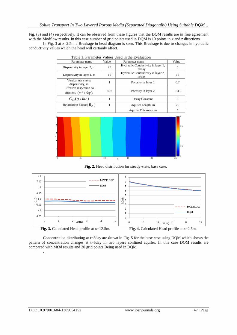
The required parameters for solving the problem are presented in Table 1. Fig. 2 shows the hydraulic

heat distribution using DQM in steady state for the first case. Head profile in z=2.5m and x=12.5m are shown in



Fig. (3) and (4) respectively. It can be observed from these figures that the DQM results are in fine agreement

with the Modflow results. In this case number of grid points used in DQM is 10 points in x and z directions.

In Fig. 3 at z=2.5m a Breakage in head diagram is seen. This Breakage is due to changes in hydraulic

conductivity values which the head will certainly affect.

Table 1. Parameter Values Used in the Evaluation Value Parameter name Value Parameter name

5 Hydraulic Conductivity in layer 1,

m/day 20 Dispersivity in layer 2, m

15 Hydraulic Conductivity in layer 2,

m/day 10 Dispersivity in layer 1, m

0.7 Porosity in layer 1 1 Vertical transverse

dispersivity, m

0.35 Porosity in layer 2 0.9 Effective dispersion so

efficient,

2( / )m day

0 Decay Constant, 1 0,( / )C g litr

25 Aquifer Length, m 1 Retardation Factor( dR )

5 Aquifer Thickness, m

0 5 10 15 20 250

1

22

33

4

5

6

6.5

7

7.5

8

z

x

Fig. 2. Head distribution for steady-state, base case.

Fig. 3. Calculated Head profile at x=12.5m. Fig. 4. Calculated Head profile at z=2.5m.

Concentration distributing at t=5day are drawn in Fig. 5 for the base case using DQM which shows the

pattern of concentration changes at t=5day in two layers confined aquifer. In this case DQM results are

compared with Mt3d results and 20 grid points Being used in DQM.

.



0 5 10 15 20 250

0.5

1

1.5

2

2.5

3

3.5

4

4.5

5

0

0.1

0.2

0.3

0.4

0.5

0.6

0.7

0.8

0.9

1

x

z

Fig. 5. Concentration distribution at t=5day.

Concentration profile is depicted in the middle of aquifer length (x=12. 5m) of the aquifer in Fig. 6 and

in Fig. 7 concentration profile in the middle of the aquifer height (z=2. 5m) is drawn. In Fig. 7 decreasing trend

can be observed during the aquifer length. The concentration value starts with a value of 1gr/lit at the left of the

aquifer and reaches to 0.329 gr/lit in the right of the aquifer. It is apparent from Fig. 6 and Fig. 7 that the present

analyses are in good agreement with Mt3d result.

Fig. 6. Calculated concentration profile at x=12.5m. Fig. 7. Calculated concentration profile at z=2.5m.

5.2 Case 2

The second case is considered to study the effect of different hydraulic conductivity values in layers on

solute transport process. All parameters except hydraulic conductivity are similar to the base case. Hydraulic

conductivity in this case for upper layer (layer2) is 5m/day and for lower layer (layer1) is intended 15 m/day.

Head profile in z=2.5m and x=12.5m are shown in Fig. 8 and Fig. 9 correspondingly by selecting 10 grid points

in DQM. In Fig. 8 it can be seen that the head in the upper region is relatively larger than the lower region at

x=12. 5m. It is indisputable that the DQM result are very close to Modflow result.


Concentration profiles at x=12.5m and z=2.5m are depicted in Fig. 10 and Fig. 11 respectively. DQM

results are in good agreement with results indicating Mt3d. It can be found that change the hydraulic

conductivity in layers that is to say the increase in hydraulic conductivity in layer 1 and reduction in the layer 2

causes an increase the Darcy velocity in layer 1 and decrease the Darcy velocity in layer 2 correspondingly.

It is noteworthy that in solving the ADE in DQM the 20 grid points were used in x and z directions.



The maximum error rates at x=0.5 are drawn in Fig. 12. The maximum error rate as percentage was

calculated as follows:

3

3

% 100Mt d DQM

error

Mt d

u uu

u

(44)

Where 3Mt du is Mt3d solution and DQMu is DQM solution


Fig. 12. Differences between Mt3d Solution and DQM Solution for the case 2 in x=12.5 at t=5day.

5.3 Case 3

In this case the porosity in layers will change. Other required parameters remain constant similar to the

base case. The porosity in layer 2 and layer 1 is assumed to be 0.7 and 0.35 respectively. Due to porosity is the

parameters affecting the ADE and has no effect on the groundwater equation. So, the solution of the

groundwater flow equation in DQM is equivalent to base case ones. To solve the ADE in DQM the 20 grid

points were used in horizontal and vertical directions. In Fig. 13 and 14 the effect of porosity change in layers is

seen. In this case the concentration is lower than the concentration in the base case at x=12. 5m. Outlet

concentration is relatively lower than the base case in z=2.5m (Fig 14).


The maximum error rates for the case 3 are shown in Fig. 15. The maximum error occurs at z=0.7m.

Fig. 15 indicates that DQM solution is close to the Mt3d result and less errors may occur in DQM result.



Fig. 15. Differences between Mt3d Solution and DQM solution for the case 3 in x=12.5 at t=5day.

5.4 Case 4

In this case hydraulic heads on both sides of the aquifer (left and right sides) are different from the

base case. In other word, all necessary parameters are considered similar to the base case except hydraulic

heads. Hydraulic heads on left and right sides will give values of 11m and 5m correspondingly. Groundwater

flow and advection dispersion equations are solved taking into account 10 and 20 points in the horizontal and

vertical directions in a parallel manner. Head profile in x=12.5m and z=2.5m are shown in Fig. (16) and Fig.

(17).

Fig. 16. Calculated head profile at x=12.5m. Fig. 17. Calculated head profile at z=2.5m.

Similar to the previous cases the ADE was solved and DQM results are depicted at x=12.5m and

z=2.5m in Fig. (18) and Fig. (19) correspondingly.


In the aquifer's inlet there is a greater difference between DQM and Mt3d results than the other points

of the aquifer. The maximum difference is 0.049 g/l that led to the creation of approximately 5.5% error rate.

Away from the entrance of the aquifer the error rates will be reduced.

5.5 Case 5

Other parameters that affect the transfer process is aquifer length. So, in this case aquifer length will

change and will be considered 50 m. Rest of parameters are similar to the parameters mentioned in base case.

Head profile is drawn in Fig. (20) and Fig. (21) at x=12.5m and z=2.5m respectively. Due to the increased



aquifer length, head values in comparison with the base case are greater than in the same place. For example, at

a x=5m head in the base case is 7.38m and in present case is 7.9m.

Fig. 20. Calculated head profile at x=12.5m. Fig 21. Calculated head profile at z=2.5m.

Concentration profiles in 5 days in x=12.5m and z=2.5m are shown in Fig. (22) and Fig. (23)

correspondingly. It is seen that with doubling the aquifer length and using the same grid points, DQM still

provides acceptable results.

Fig. 22. Calculated concentration profile at x=25m. Fig. 23. Calculated concentration profile at z=2.5m.

Maximum error rates at x=25m (center line) are depicted in Fig. (24). Maximum error rate occurred in

this case has slaked from the aquifer entrance and finally this error reach to zero in the end of the aquifer.

Fig. 24. Differences between Mt3d Solution and DQM solution for the case 3 in x=25m at t=5day.

VI. conclusion As a result, the weighting coefficients of the first-order derivative are determined by a simple algebraic

formulation without any restriction on choice of grid points, and the weighting coefficients of the second and

higher-order derivatives are determined by a recurrence relationship. This is a major breakthrough in the

development and application of the DQ method. Since then, the DQ method has been extensively applied to

solve the fluid flow problems and the structural and vibration problems. So to cover all fields by DQM, in this

paper the application of the DQM in solving the contaminant transport in layered confined aquifer was

discussed. Five cases are considered to study the effect of various parameters in the transfer process. The 10 and

20 grid points are used in this study for solving the groundwater and transport equation correspondingly. The



comparisons show lower error values, less computational time, rapid convergence than the other numerical

methods while a good agreement with the exact results.

References [1] U. Y. Shamir, D. R. E. Harleman. Dispersion in layered porous media. Proceedings of ASCE, Journal of the Hydraulics Division,

93, 1967, 237–260.

[1] ANS. Alniami, KR. Rushton. Dispersion in stratified porous media: analytical solutions. Water Resources Research., 15(5), 1979, 1044–1048.

[2] FJ. Leij, JH. Dane, MT. Van Genuchten. Mathematical analysis of one-dimensional solute transport in a layered soil profile. Soil

Science Society of America Journal., 55(4), 1991, 944–953. [3] FJ. Leij, MT. Van Genuchten. Approximate analytical solutions for solute transport in two-layer porous-media. Transport in Porous

Media, 18(1), 1995, 65–85.

[4] Y-C. Li, PJ, Cleall. Analytical solutions for advective-dispersive solute transport in double-layered finite porous media. Int. J. Numer. Anal. Meth. Geomech., 35(4), 2011, 438-460.

[5] R. E. Bellman, J. Casti. Differential quadrature and long-term integration. Journal of Mathematical Analysis and Applications, 34,

1971, 235-238. [6] C. Shu, B. C. Khoo, K. S. Yeo, Y. T. Chew. Application of GDQ Scheme to Simulate natural Convection in A Square Cavity. Int.

Commun. heat and Mass Transfer, 21(9), 1994, 809-817.

[7] C. Shu, B. E. Richards. Application of generalized differential quadrature to solve two-dimensional incompressible Navier-Stokes equations. Int. J. Numer. Methods Fluids, 1992, 15, 791-798.

[8] C. Shu, B. C. Khoo, K. S. Yeo K. S. Numerical solution of incompressible Navier-Stokes equations generalized differential

quadrature. Finite Element in Analy. Design, 18, 1994, 83-97. [9] C. Shu, H. Xue. Explicit Computation of Weighting Coefficients in the Harmonic Differential Quadrature. J. Sound and Vibration.,

204(6), 1997, 549-555. [10] C. Shu, Y. T. Chew. Fourier Expansion-Based Differential Quadrature and Its Application to Helmholtz Eigenvalue Problems. J.

Commun. Numer. Meth. Eng., 13(11), 1997, 643-653.

[11] C. Shu, H. Ding, K. S. Yeo.Local radial basis function-based differential quadrature method and its application to solve two-dimensional incompressible Navier–Stokes equations. J. Comput. Methods Appl. Mech. Eng., 192, 2003, 941–954.

[12] C. Shu, H. Ding, H. Q. Chen, T. G. An upwind local RBF-DQ method for simulation of inviscid compressible flows. Comput.

Methods Appl. Mech. Eng., 194, 2005, 2001-2017. [13] C. Shu, B. C, K. S. Yeo, Y. T. Chew. Application of GDQ Scheme to Simulate natural Convection in A Square Cavity.” Int.

Commun. heat and Mass Transfer, 21(9), 1994, 809-817.

[14] C. Shu, H. Ding, H. Q. Chen, T. G. Wang. An upwind local RBF-DQ method for simulation of inviscid compressible flows. Comput. Methods Appl. Mech. Eng., 194, 2005, 2001-2017.

[15] C. H. Tsai, D. L. Young, C. C. Hsiang. The localized differential quadrature method for two-dimensional stream function

formulation of Navier–Stokes equations. Engineering Analysis with Boundary Elements., 35, 2011, 1190–1203. [16] X. Wang, L. Gan, Y. Zhang. Differential quadrature analysis of the buckling of thin rectangular plates with cosine-distributed

compressive loads on two opposite sides. J. Advan. Eng. Software., 39(8), 2008, 497–504.

[17] F. Civan. Rapid and accurate solutions of reactor models by the quadrature method. Computers & Chemical Engineering., 18, 1994, 10005-10009.

[18] H. Li, S. Mulay. 2D simulation of the deformation of pH-sensitive hydrogel by novel strong-form meshless random differential

quadrature method. Comput Mech., 48, 2011, 729–753. [19] A. A. Mahmoud, R. Awadalla, M. M, Nassar. Free vibration of non-uniform column using DQM. Mechanics Reaserch

communication., 38, 2012, 443-448.

[20] M. Danesh, A. Farajpour, M. Mohammadi. Axial vibration analysis of a tapered nanorod based on nonlocal elasticity theory and differential quadrature method. Mechanics Research Communications., 39, 2012, 23– 27.

[21] R. P. Chen,W. H. Zhou, H. Z. Wang, Y. M. Chen. One-dimensional nonlinear consolidation of multi-layered soil by differential

quardrature method. Computers and Geotechnics, 2005, 32, 358-369. [22] M. Char, F. Chang, B. Tai. Inverse determination of thermal conductivity by differential quadrature method. International

Communications in Heat and Mass Transfer, 35, 2008, 113-119.

[23] B. Kaya, Y. Arisoy, Differential quadrature method for one-dimensional aquifer flow. Math. Comput. Appl. 16(2), 524 2011. [24] A. Robati, GA. Barani. Modeling of water surface profile in subterranean channel by differential quadrature method (DQM), Appl.

Math. Mod. 2009, 33: 1295-1305.

[25] B. Kaya, Y, Arisoy.Differential Quadrature Method for Linear Long Wave Propagation in Open Channels. Wave Propagation in Materials for Modern Applications, 2010, A.

[26] B. Kaya, Y, Arisoy, A. Ulke. Differential Quadrature Method (DQM) for Numerical Solution of the Diffusion Wave Model.” J.

Flood Eng., 2010, 1(2). [27] C. W. Bert, M. Malik. Differential quadrature method in computational mechanics, a review. Appl. Mech. Rev., 49, 1996, 1-27.

[28] C. Shu. Differential Quadrature and its Application in Engineering. (Springer, Londen, 2000).

[29] J. O. Mingle. Computational considerations in nonlinear diffusion. Inter. J. Numer., Methods Engrg., 7, 1973, 103-116. [30] F. Civan. Rapid and accurate solutions of reactor models by the quadrature method. Computers & Chemical Engineering., 18,1994,

10005-10009.

[31] J. R. Quan, C. T. Chang. New insights in solving distributed system equations by the quadrature method-1. Comput. Chem. Energy, 13, 1982, 779–788.

[32] C. Shu, B. E. Richards. Application of generalized differential quadrature to solve two-dimensional incompressible Navier-Stokes

equations. Int. J. Numer. Methods Fluids, 1992, 15, 791-798. [33] C. W. Bert, X. Wang, A. G. Striz. Differential quadrature for static and free vibrational analysis of anisotropic plates. Int. J. Solids

Structures, 30, 1993, 1737-1744.

[34] W. Chen, Y. Yu. Calculation and analysis of weighting coefficient matrices in differential quadrature., Proc., of the 1st Pan-Pacific Conference on Computational Engineering, Elsevier Science Publ. B. V. , Netherlands., 1993, 157-162.

[35] B. Kaya and Y. Arisoy, “Differential quadrature solution for one-dimensional aquifer flow,” Math. Comput. Appl. 16(2),

524 (2011)

solute transport in two layered porous media … dqm to solve three one-dimensional aquifer flow...

Documents