a theory of satisfaction and utility with empirical and ... · a measure of pleasure and pain. it...
TRANSCRIPT

1
A Theory of Satisfaction and Utility with Empirical and Experimental Evidences*
Louis Lévy-Garboua
Centre d’économie de la Sorbonne, Université de Paris I (Panthéon-Sorbonne), and CIRANO
Claude Montmarquette
Université de Montréal and CIRANO
AFSE-JEE
LYON 2007
* We thank the Bell University Laboratory for their financial support. We are grateful to Julie Héroux and Nathalie Viennot-Briot for their competent help in conducting this research. Any remaining errors are ours.

2
I. Introduction
People often express judgments of satisfaction or dissatisfaction towards their own past experience
of a brand, a film, their job, the incumbent government, and even their whole life. These judgments,
which are often much easier to collect than objective data, have been widely used by psychologists,
political scientists, and consumer studies for predicting repeat purchases of a brand or electoral
outcomes, and for describing the happiness or “subjective well-being” (SWB) of various segments of
the population. However, the bulk of satisfaction and happiness research emphasizes the reference-
dependence of the satisfaction variable (for a recent survey of the psychological literature on SWB, see
Diener et al. 1999), a result which stands in sharp contradiction with the conventional economic
analysis of utility as a preference index. This may help explain why most economists, with a few
prominent early exceptions (Easterlin 1974, Hamermesh 1977, Freeman 1978, Borjas 1979), have
long felt unable to extract reliable information from subjective data of this kind. Fortunately, we
believe, there are signs that the situation is now rapidly changing since the publication of a few
influential papers (Clark and Oswald 1996, Kahneman, Wakker and Sarin 1997, Frey and Stutzer
2002). These papers, among others, have contributed to a better recognition by economists that
satisfaction judgments were meaningful. However, we are still concerned that these papers take the
identification of “satisfaction” with “utility” for granted, although until very recently the
psychological literature on SWB did not commonly refer to “utility”.1 Such bold translation of SWB
into utility is questionable and has far-reaching implications for economic analysis. The best known
illustration of what we mean is that, if satisfaction and utility are just the same thing, Easterlin’s
(1974, 1995) observation that raising the incomes of all does not increase the happiness of all does
demonstrate that utility is a function of relative income, since the latter is not affected by uniform
economic growth.2 Even though the economics profession is increasingly receptive to psychological
insights (e.g. Rabin 1998), we doubt that many are ready to accept all the welfare implications of
relative utility. Kahneman et al. (1997) solve this theoretical puzzle by making a distinction between
decision-utility and experienced utility. They refer to decision-utility as a preference index describing
how choices are made and to experienced utility as the measure of pleasure and pain suggested by
Bentham (1789). Consequently, they postulate the existence of two very different meanings for 1 Diener et al.(1999) never mention the word “utility” in their extensive survey on SWB. 2 Although Easterlin’s early conclusions have recently been challenged on larger cross-national data sets (see Veenhoven 1996, Diener et al. 1999: 287-289), it is by now a widely held view that the individual’s ranking in the income distribution of an economy, or relative income, has a significant, and typically greater, impact on the level of happiness than absolute income.

3
“utility” and show experimentally that experienced utility, unlike decision-utility, is not being
maximized. However, the conceptual meaning of experienced utility, or pleasure and pain, remains
unclear in their approach.
The theoretical contribution of this paper is to propose a more complete, yet more parsimonious,
solution to the satisfaction puzzle. The latter is consistent with Kahneman et al.’s (1997) contention
that experienced utility should not be confused with decision-utility but it strictly follows the
economic usage of defining “utility” as a preference index. We jointly define here decision-utility as
the ex ante utility, and experienced utility as the ex post utility, that both associate to a single preference
relation. In a truly predictable world, the ex ante utility would always coincide with the ex post utility
and this distinction would not matter. But the real world is full of surprises and the experienced utility
of a brand or of a job often differs from the decision-utility even if the latter led to the prior choice
of that brand or job. The surprises that occurred since the experience began make the difference. Ex
post utility is conditional on the experienced contingencies that were unexpected when the decision
was made or the experience began. This definition of experienced utility has the obvious advantage
of being simple and natural for an economist. We also refer to “satisfaction” and “dissatisfaction” as
a measure of pleasure and pain. It will be argued in general, as suggested in our earlier work on job
satisfaction (Lévy-Garboua and Montmarquette 2004), that satisfaction judgments and feelings after
a specific experience relate to, but do not coincide with, the ex post utility of that experience in that
they manifest the experienced preference for the experienced action relative to available alternatives. In
simple words, reporting one’s satisfaction is the judgment that one would wish to repeat one’s past
experience if one could choose again.
Since preferences involve comparisons, satisfaction judgments and feelings which reflect this
experienced preference must be relative. Thus the reference-dependence of satisfaction judgments
and feelings does not require that an individual’s utility function be reference-dependent as well. The
findings and discourse of psychologists about the reference-dependence of satisfaction judgments
and feelings may be reconciled with the conventional economic analysis of utility as a preference
index. This has the further consequence that human feelings and subjective well-being should be
measured on ordinal scales.
The economic interpretation of satisfaction judgments and feelings given here offers many
interesting predictions regarding satisfaction judgments. We can explain, for instance, why so many
persons usually report themselves as happy or satisfied (e.g. Campbell 1981, Diener and Diener
1996); why even large shocks may not cause large and lasting effects on satisfaction and happiness in

4
the future ( Brickman and Campbell 1971 and Kahneman 1999 speak of “treadmill effects”); why
raising the incomes of all does not necessarily increase the happiness of all (Easterlin 1974, 1995;
Diener and Suh 1997; Oswald 1997); and why satisfaction is so much dependent on our capacity to
choose what we like and revise our decisions in case of need. We feel that this last implication has
not fully received the emphasis that it deserves in the literature, and thus we provide new empirical
evidence that differences in average life satisfaction across countries can be largely attributed to
differences in economic and political freedom.
Another objective of this paper is to comfort some of the empirical evidences with experimental
data. But, above all, we mobilize the experimental economic approach to test our theoretical views
on satisfaction that cannot be easily test otherwise.
Section II develops the theory of satisfaction judgments and feelings as an experienced preference
and derives the main properties of the former. Section III shows that the theoretical predictions
conform to a number of robust findings of the literature on SWB. We emphasize here the major
influences of freedom of choice and experienced utility gaps (i.e. the difference between what
happened and what might have happened) on satisfaction. Section IV shows empirical evidence that
life satisfaction is less dependent on GDP per capita than on indicators of the freedom of choice, as
forcefully argued by Sen (1999). Section V discusses the results of our experiment on satisfaction.
Section VI concludes.
II. A theory of satisfaction
There is an “obvious” theory of satisfaction judgments and feelings, which simply identifies the
latter (SWB) with “utility” (U):
USWB ≡ .
This theory is seldom taken literally. For instance, Clark and Oswald (1996) refer to a social utility,
Frey and Stutzer (2002) to a procedural utility, and Kahneman et al. (1997) to a hedonic notion of
utility suggested by Bentham (1789) and later discarded by economists. It is not very clear whether
these utility functions should be the same and how they relate to actual decisions. However, in order
to demonstrate that SWB is an economic variable, it is necessary to relate the latter to decision-
utility. In marketing research, consumers’ satisfaction is taken as a good predictor of repeat
purchases of the experienced product. In political science, citizens’ satisfaction with political leaders
or the incumbent government is taken as a good predictor of their future election or reelection. In
labor research, job satisfaction is taken as a good predictor of job mobility (e.g. Freeman 1978). In
5
social psychology as well, inequity feelings are thought to give rise to decisions that will reduce
inequity (Adams 1963). The problem is that none of these contentions, which have received
extensive empirical confirmation, can be seen as a straightforward prediction of the simple theory of
satisfaction-as-utility. Although a satisfying experience may often yield high utility, a high-utility
good would only be chosen if it yielded more utility than available alternatives. Moreover,
competition normally entails the availability of alternative goods yielding high utility as well, so that
high utility per se cannot explain the positive correlation between consumers’ satisfaction and repeat
purchases of an experienced good. An experienced good will be repeatedly purchased by rational
consumers only as long as it is experience-preferred to the best opportunity.
Thus a more economically-relevant definition of satisfaction judgments and feelings is the following.
The latter elicit the experienced preference for one good or bad over available alternatives. The
present notion of experienced preference is quite as flexible as the more familiar notion of decision-
preference. It is not restricted to the real experience of one brand or job but extends to anticipated
options available in the future, just like decision-preference does, and furthermore to mental
experiences of past options that might have been chosen but were eventually discarded. In the
present paper, we make the simplifying assumption of perfect memory. The latter hypothesis may
serve as a good starting point since it is in line with the concept of “autobiographical self” that
Damasio (1999) derived from evidence on neurological pathologies and direct observation of the
brain.3 Thus we might restate that satisfaction judgments and feelings elicit the decision-preference
of the autobiographical self. Since the individual is supposed to make an ex post comparison of her
own experience with what it might have been, her satisfaction manifests a feeling of regret-rejoicing.4
We formally define satisfaction or subjective well-being derived from an experienced good z as an
ordinal variable taking discrete values. If individuals only compare their own situation with a single
alternative, the satisfaction judgment or feeling is a binary variable (not satisfied-satisfied)
3 Damasio (1999: 174) suggests that the following mental evaluation process is being continually implemented in the brain by what he calls the “autobiographical self”: “The autobiographical self is based on autobiographical memory which is constituted by implicit
memories of multiple instances of individual experience of the past and of the anticipated future. The invariant aspects of an individual’s biography form the basis for autobiographical memory. Autobiographical memory grows continuously with life experience but can be partly remodelled to reflect new experiences. Sets of memories which describe identity and person can be reactivated as a neural pattern and made explicit as images whenever needed. Each reactivated memory operates as a “something-to-be-known” and generates its own pulse of core consciousness. The result is the autobiographical self of which we are conscious.”
4 This is not to be confused with the ex ante feeling of regret-rejoicing sometimes invoked in the analysis of decision under risk.

6
)()(1 ∗≥= zUzUifSWB
(1)
)()(0 ∗<= zUzUif
where ∗z designates the mentally experienced alternative and U is the individual’s utility function.
The continuous latent variable,
(2) )()(),( ∗∗∗ −≡ zUzUzzSWB , (
enables us to rewrite the satisfaction function as
0),(1 ≥= ∗∗ zzSWBifSWB
(3)
0),(0 <= ∗∗ zzSWBif
We contend that the SWB functions which can be estimated either from self-reports or by
objectively measuring emotions (Kahneman 2001) reflect such experienced utility gaps. ∗SWB describes
the feeling of pleasure and pain and relates it to the preference-based definition of utility used in
modern economics. ),( ∗zzSWB defines the satisfaction function of the individual with respect to the
objects of choice z at a given date conditional on the reference ∗z .
Treating satisfaction as an experienced preference is no more difficult than treating it as an
experienced utility but yields more and better predictions, as will appear in later sections. The price
to be paid is that researchers must give up the hope of directly measuring utility, but this is partly
compensated by the possibility of measuring other unobservable variables at the individual level like
pleasure and pain (Kahneman et al. 1997) or the propensity to quit the present job (Lévy-Garboua,
Montmarquette and Simonnet 2007). Our approach to satisfaction is related to those of Festinger
(1957) and Adams (1963) for social psychology or Michalos (1980) for social indicators research. For
example, psychologists treat equity as a specific form of outcome satisfaction arising in social
interactions. Adams (1963) defines inequity by the dissonance between a person’s experience (say
her perceived wage rate) and her normative expectation (the fair wage). He then follows Festinger’s
(1957) contention that people react to cognitive dissonance when their experience does not conform

7
to their normative expectation.5 Satisfaction, like inequity, is generated by the dissonance between
experienced utility of a good or bad and its normative expectation. The magnitude of dissonance is
well captured by the experienced utility gap (2), which is the difference between experienced utility
and its normative expectation. When normative expectations are met by the experienced outcome,
the experienced utility gap is positive and people are satisfied with the outcome. On the other hand,
when experienced outcome falls short of normative expectations, the experienced utility gap is
negative and people are dissatisfied with the outcome. The various types of pleasure caused by
satisfaction and the various types of pain caused by dissatisfaction define just as many types of
tension which drive the person to reduce them by the most appropriate action. The various types of
tension define specific emotions, as Zajonc (1980) notes that many emotions function like a drive
commanding one’s current preferences and generating a context-dependent motivation to act
accordingly. The correspondence between emotions and drives, and between drives and immediate
actions, points at the preference-like nature of emotions. Emotions are functional in driving new
decisions, which is consistent with Damasio’s (1994) contention that Descartes’ error was to
dissociate rational decision from emotions. Damasio observed that a man who had kept his
reasoning ability but lost his emotions after a commotion eventually made bad decisions because he
lacked the emotional response, in other words the actual preference, which would drive him to take
the decision that his own reason prescribed.
PROPOSITION 1. Satisfaction with respect to a vector of goods elicits the preference of the autobiographical self
for the vector of outcomes truly experienced by the individual relative to at least one mentally experienced vector of
reference outcomes.
The main result of this paper is that feelings must differ from utility when the latter is defined as a
preference index and they manifest experienced preferences. Consequently, we believe that utility
analysis is often immune from the reference-level effects concerning human satisfaction or well-
being to be found in the psychological literature.
Two features of reference-dependence that have been identified in a wide variety of domains are
loss aversion and diminishing sensitivity to outcomes, which Tversky and Kahneman (1991) derive
5 Adams (1963:467) writes: “(a) The presence of inequity in Person creates tension in him. The tension is proportional to the magnitude of inequity present. (b) The tension created in Person will drive him to reduce it. The strength of the drive is proportional to the tension created; ergo, it is proportional to the magnitude of inequity present.”

8
from the basic laws of perception. Loss aversion is the assertion that people often exhibit
substantially more negative reactions to a small loss than they show positive reactions to a same-
sized gain. Diminishing marginal sensitivity to outcomes is the assertion that changes in any
direction close to one’s reference level are more strongly felt than changes further away. The present
theory of satisfaction derives both similar and different implications from the stepwise shape of the
satisfaction function, which are summarized by the following proposition.
PROPOSITION 2
Holding one reference level constant, there is an asymmetry of satisfaction feelings with respect to one-dimensional gains
and losses from an initial position in the vicinity of this reference level. When the initial position lies slightly above the
reference level (which is then an opportunity level), it is immediately felt an aversion to moderate losses but no attraction
to gains of equal size. However, the sensitivity of dissatisfaction to losses diminishes with the size of loss. When the
initial position lies slightly under the reference level (which is then an aspiration level), it is immediately felt an
attraction to moderate gains but no aversion to losses of equal size. However, the sensitivity of satisfaction to gains
diminishes with the size of gain.
If there is a finite number of reference levels, satisfaction increases or decreases by steps. It makes a discrete jump
upward (downward) each time the situation becomes better (worse) than one of the options and stay flat between two
consecutive options.
Proof: See Appendix.
III. Implications of the theory for satisfaction judgments
1. Treadmill effects
Following Brickman and Campbell (1971) and Kahneman (1999), we shall speak of “treadmill
effects” when current shocks, even large, do not cause large and lasting effects on satisfaction and
happiness. The early evidence by Easterlin (1974) that sustained economic growth does not increase
the average level of happiness may be the best known example of a treadmill effect in the economic
literature. The prevalence of treadmill effects is attested by the finding that “bottom-up” factors like
current external circumstances account for a small share of the variance in SWB reports (Argyle
1999, Diener et al. 1999). SWB is moderately stable across the life span, so that it has come to be

9
viewed by “top-down” theories as a personality trait (Diener and Lucas 1999).6 These results actually
derive from equation (2) if past experiences are unobservable in surveys and weight more heavily
than current data. Moreover, to the extent that an individual’s personality is partly acquired and
shaped by her life antecedents, the unobservable heterogeneity of past experience may capture part
of what is attributed to personality in the “top-down” theories of SWB.
Indeed, several kinds of treadmill effects are predicted by equation (2). They result from the
reference-dependence of satisfaction, from the role and weight of past experience, and from the
length of the average life expectancy. For instance, uniform economic growth would have little
effect on experienced utility gaps because it keeps on raising both actual incomes and market
opportunities alike. An external shock that similarly affects, after a brief transition period, both the
individual’s situation and his opportunities in the future will have only a minor impact on
satisfaction. This is exactly what is to be expected from, say, winning a lottery or becoming a
paraplegic after an accident and, indeed, Brickman et al. (1978) found that, after a period of
adjustment, lottery-winners were hardly happier and paraplegics hardly less happy than a control
group. Here, a permanent shock on utility levels results in a temporary shock on utility gaps. i.i.d.
temporary shocks affecting current outcomes and options repeatedly would also leave average
satisfaction virtually unchanged. For instance, the temporary pleasure of watching a good play is
randomly distributed and does not convey to future plays as each play is usually seen once. Lévy-
Garboua and Montmarquette (1996) found that experienced theatre-goers reported liking the last
play they saw with the same frequency than inexperienced spectators although general theatre
appreciation scores correlated with experience of theatre. Both good and bad surprises do not have
much effect on satisfaction in the long run when they equally affect the utility of actual experience
and alternatives.
Even when this is no longer true, the effect of bad surprises on experienced utility can sometimes
be offset by a revision of choice (e.g., a bad job match can be offset by quitting the job) if there is
enough time ahead of us. This has the intriguing implication that some components of satisfaction
like satisfaction with job (Hamermesh 1977, Clark et al. 1996, Lévy-Garboua and Montmarquette
1998) and marriage (Argyle 1999) may eventually increase with age. The explanation runs as follows.
6 The psychological literature distinguishes between “top-down” and “bottom-up” factors affecting SWB. Bottom-up factors are external and objective factors like the experience of pleasant or unpleasant events and socio-demographic variables (e.g., age, gender, education, income, and marital status). Top-down factors are internal and subjective factors, like personality or adaptation and coping processes, that determine how events are perceived (see Diener et al.(1999 ) for more details).

10
Rational workers will keep moving to what they expect to be the best job and cannot systematically
make wrong predictions in the long run, under rational expectations. Thus, provided a significant
share of workers is able to capture rents on their job, the average present value of past wage gaps
will remain permanently positive after a sufficient number of years (and jobs). The future
component will stabilize with experience as a result of learning and eventually converge in
probability towards zero as the duration of the remaining life at work declines. The upward-sloping
relationship of job satisfaction with age, which results from the combination of these two effects, is
obtained in the long run. It is not necessarily monotonic over the life cycle and may be U-shaped.
The foregoing analysis can easily be replicated for marriage.
2. Most people are happy
A stylized fact of studies of satisfaction judgments is that responses are typically concentrated in
the upper segments of the satisfaction scale (e.g., Campbell 1981, Diener and Diener 1996). Most
people usually report that they are happy or pretty happy! For instance, Sousa-Poza and Sousa-Poza
(2000) compare average levels of job satisfaction between 21 developed countries and find a high
level of satisfaction in all countries, with an unweighted average of 78.7% reporting themselves in
the top-three levels of a seven-point scale. 7 This fact would be hard to explain in the satisfaction-as-
utility framework. By contrast, its interpretation is illuminating in the experienced preference
framework. The rationality assumption implies that, under certainty, individuals will always be
satisfied with choices they deliberately made. If experienced utility coincided with decision-utility, all
rational decision-makers would be fully satisfied with their choices. Under dynamic uncertainty,
however, experienced utility will not generally coincide with decision-utility so that experienced
utility will not be generally maximized by the actual choice of rational individuals. In short,
satisfaction judgments and feelings reveal how far experienced utility has been maximized! The high
scores of satisfaction and happiness, which are commonly observed, indicate that people often
experience the outcomes of their own choices and that the incidence of bad surprises is fairly
limited. The low incidence of bad surprises upon satisfaction in the long run is caused by treadmill
effects.
7 They analyzed the data set on Work Orientations from the 1997 International Social Survey Program. All countries used the same wording for the job satisfaction question and the same seven-point scales for reporting individual answers.
11
3. Satisfaction and the freedom of choice
The variability of satisfaction judgments across domains in the aggregate mainly reflects the degree of
freedom of individual choices which characterizes each of these domains. Market goods usually get
higher satisfaction scores from customers in market economies than do governments from citizens
in democratic regimes. The reason is presumably that market goods are privately chosen by all
consumers while governments are only chosen by the median voters. More generally, satisfaction
with private domains of life (health, housing, marriage and work) is typically higher than satisfaction
with public matters, at least in modern western nations (Veenhoven 1996). People in these nations
are certainly freer to choose for themselves than for society. But they are also freer to choose for
society the more democratic is the society. Frey and Stutzer (2000) show on a sample of Swiss
residents that direct democratic rights ( which vary across the 26 cantons) raise happiness and they
also attribute the lower score of foreigners to the fact that the latter are deprived of the right to vote.
Other convincing evidence is the fact that respondents report greater overall job satisfaction than
pay satisfaction. The mean scores (standard deviations) found by Clark and Oswald (1996, data
appendix) on a 1-7 scale were respectively 5.50 (1.51) and 4.49 (1.95). A suggested interpretation is
that individuals control their job as a whole better than their pay, because choosing a job is a
package deal whose single elements, like pay, cannot be separately and therefore, in most practical
instances, freely chosen. The same argument runs, of course, for other attributes of the job.
People tend to be less satisfied on average with experiences out of their control. To some extent,
the sense of control is dictated by personality. Extraversion is associated with the personal ability to
control one’s environment and with positive affect, while introversion and neuroticism go with a
loss of control and negative affect. For instance, Veenhoven (1996: 27) makes the point explicit:
“With respect to personality, the satisfied tend to be socially extravert and open to experience. There is
a notable tendency towards internal control beliefs, whereas persons who are dissatisfied tend to feel
they are a toy of fate. Much of the findings on individual variation in life-satisfaction boil down to a
difference in ability to control one’s environment.”
At the macro level, unemployment and inflation rates, which have been found to adversely affect
reported happiness (Di Tella et al. 2001), are two bads beyond individual control. At the micro level,
persons who lost their employment are less happy, holding income and other individual traits
constant (Clark and Oswald 1994, Gerlach and Stephan 1996, Winkelmann and Winkelmann 1998),
and it is argued here that the measured fall in happiness indicates to what extent unemployment was

12
involuntary. Consequently, job satisfaction studies provide evidence of job rationing in the labor
market.
All of these findings are immediately implied by a choice-theoretic interpretation of reported
satisfaction and happiness like ours, while they remain mere “facts of life” under the more
traditional view of satisfaction as utility.
IV. Empirical evidence on satisfaction and the freedom of choice
We present earlier in the section satisfaction and the freedom of choice, Veenhoven (1996: 27)
makes the point explicitly that ‘Much of the findings on individual variation in life-satisfaction boil
down to a difference in ability to control one’s environment.’
Given the importance of this prediction of the present model and its relative neglect by other
models, we give an empirical illustration of the profound impact that the freedom of choice in all
compartments of life can have on life satisfaction. We gathered statistics on life satisfaction,
economic freedom, political and social freedom, and GDP per capita (in PPP), for 40 countries and
three years (1985, 1990, 1995). A detailed account of sources and methods is provided in Appendix.
Life satisfaction is taken from three waves of the World Values surveys, which address adults of 18
and over in 45 societies. It is measured for each respondent on a 10-point scale by increasing order
of satisfaction, and a national average is then computed for each year. To make data as comparable
as possible, we follow Diener et al. (1995) by taking standardized values for the three years. A nation-
wide index of political and social freedom is being published annually since 1972 by Freedom
House. This index averages political rights and civil liberties on a number of dimensions, each
measured on a 7-point scale. We inverted this scale so as to rank freedom by increasing order.
Countries rating 1-2.5 on the freedom scale are generally considered as “not free” and countries
rating 5.5-7 are considered as ‘free”, with countries rating in the intermediate range 3-5.5 being
considered as “partly free”. We were able to add the recently published index of economic freedom
provided by Gwartney and Lawson (2002) in order to complete the range of domains for which
freedom of choice is being apprehended.
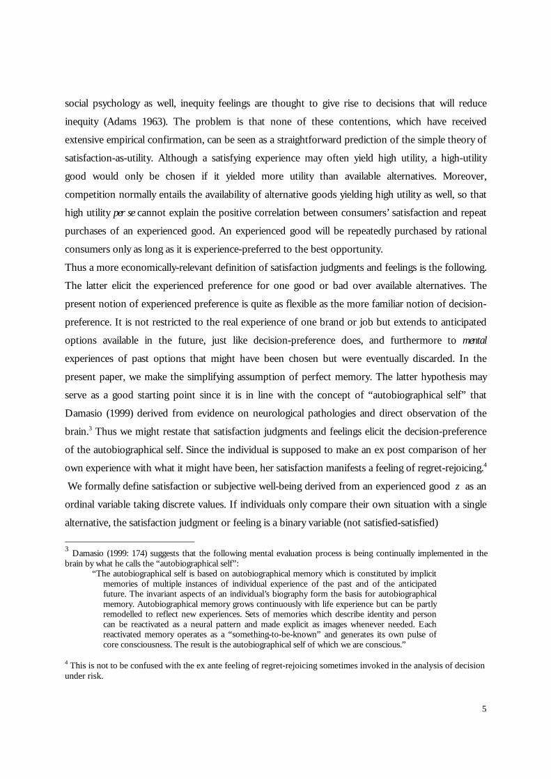
Figure 1 plots life satisfaction, measured as deviation from the mean) against GDP per capita for the
75 country-year observations for which all of these indexes were available. This sample of countries
and years is wider than the one considered by Veenhoven (2000) and reproduced by Frey and
Stutzer (2002) which was restricted to 38 mainly developed countries at the beginning of the 1990s.
Moreover, Veenhoven’s study is concerned with happiness rather than life satisfaction. At first

13
glance, a rising concave relationship can be seen. However, three groups of countries can be sharply
distinguished on the figure, which are signaled by different colors: developed market economies (49
observations in blue), developing market economies (23 observations in pink), and planned or
centralized economies (23 observations in yellow). Obviously, for its greatest part, the positive
correlation between life satisfaction and income is spurious and caused by the unusually low level of
life satisfaction in planned or centralized economies. Table 1 confirms the diagnosis by showing that
economic and political or social freedom correlate with income and even more strongly correlate
with life satisfaction. Planned and underdeveloped market economies have very comparable incomes
on average and much lower incomes than developed market economies. However, the difference in
life satisfaction between developed and underdeveloped market economies is only one-third of what
it is between developed and planned economies. A closer inspection of table 1 suggests that
economic freedom is on average even more important than political or social freedom in
determining life satisfaction. The results exhibited by table 1 and figure 1 are so clear that we believe
that they are robust. The freedom of choice is likely an essential determinant of life satisfaction at
least as much as economic freedom is an essential determinant of income growth. Freedom might
well be, through all its manifestations, the most important determinant of development in the broad
sense advocated by Sen (1999).
14
Figure 1: Life satisfaction and per capita income across countries, 1985-1995
-3,00
-2,50
-2,00
-1,50
-1,00
-0,50
0,00
0,50
1,00
1,50
2,00
0,00 5000,00 10000,00 15000,00 20000,00 25000,00 30000,00
GDP Per Capita (International $, PPP)
L i f e S a t i s f ac t i on
A : Market Oriented, B : Market OrientedD D l iCentralized

15
Table 1 Average indicators for non-market and market economies by level of development, 1985-
1995
Countries Life Satisfaction
GDP Per Capita
Political Freedom
Economic Freedom
No Obs.
Developed Market Economies
1985-1995 0,48 16316,46 6,61 6,88 49
1985 0,30 12414,74 6,20 6,53 19
1990 0,62 17039,00 6,50 6,94 20
1995* 0,58 22284,67 6,95 7,44 10
Developing Market Economies
1985-1995 -0,05 5070,99 4,37 5,03 23
1985 -0,33 3730,00 4,26 4,46 7
1990 0,02 5081,25 4,46 4,84 8
1995 0,19 6234,09 4,37 5,72 8
Non-market Economies
1985-1995 -1,09 5226,80 3,78 4,08 23
1985 -1,33 4575,00 4,43 4,11 4
1990 -1,15 5094,55 3,63 3,62 11
1995 -0,89 6597,06 3,67 4,71 8
Life satisfaction: All things considered, how satisfied are you with your life as a whole these days? (on a scale from 1 to 10, where 1 = dissatisfied, 10 = satisfied). Data for 1990 and 1995 were standardized to be compatible with Diener et al’s (1995). World Values Study Group (1994). World Values Survey, 1981-1984, 1990-1993, and 1995-96. GDP per capita in international $, PPP: World Bank. Main indicators. Political and Social Freedom: Average of political rights and civil liberties ratings. Countries whose ratings average 1-2.5 are generally considered "Free," 3-5.5 "Partly Free," and 5.5-7 "Not Free. We use the continuous variable (7.7 - the country’s rating) to measure the countries’ Political and Social Freedom. Freedom House (2001). Freedom in the World Country Ratings, 1972-73 to 2000-01. Economic Freedom: A chain-weighted summary index measuring the degree of economic freedom present in 5 major areas: Size of Government (expenditures, taxes and enterprises); Legal Structure and Security of Property Rights; Sound Money; Freedom to Trade with Foreigners; Regulation of Credit, Labor, and Business. The Index varies from 0 to 10, with high score meaning more economic freedom. Economic Freedom of the World: 2002 Annual Report, by J. Gwartney and R.Lawson. List of countries: Developed market economy:
16
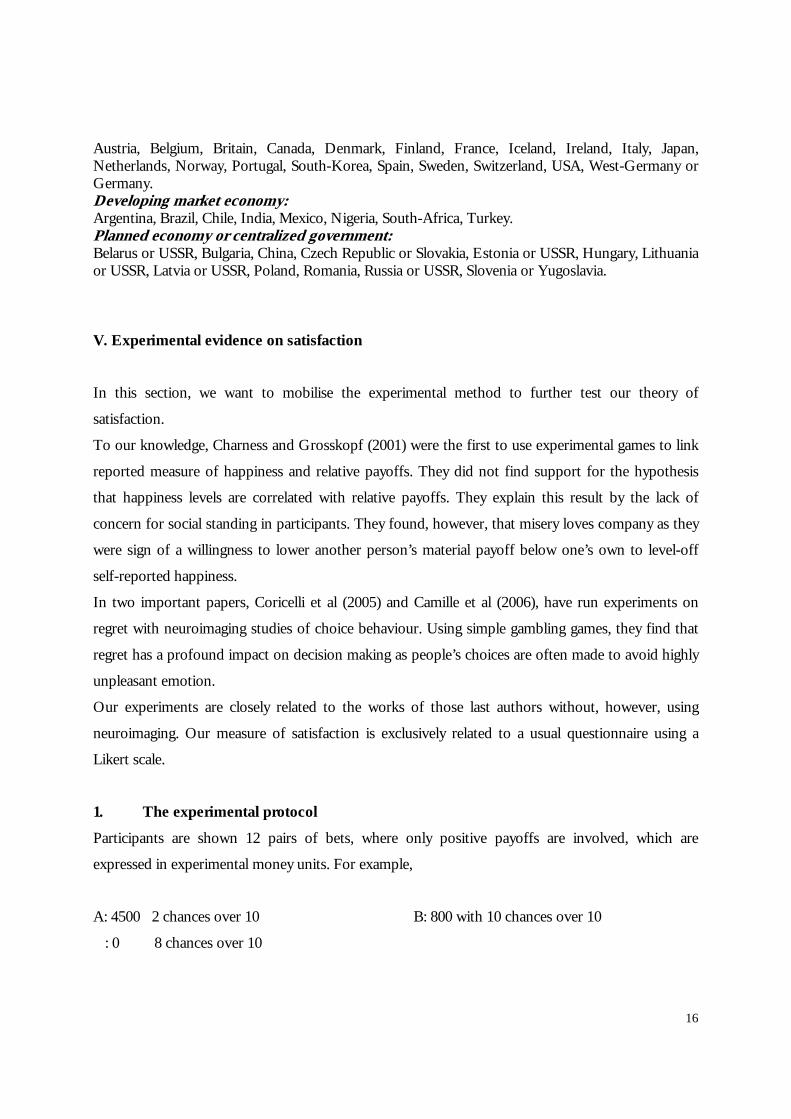
Austria, Belgium, Britain, Canada, Denmark, Finland, France, Iceland, Ireland, Italy, Japan, Netherlands, Norway, Portugal, South-Korea, Spain, Sweden, Switzerland, USA, West-Germany or Germany. Developing market economy: Argentina, Brazil, Chile, India, Mexico, Nigeria, South-Africa, Turkey. Planned economy or centralized government: Belarus or USSR, Bulgaria, China, Czech Republic or Slovakia, Estonia or USSR, Hungary, Lithuania or USSR, Latvia or USSR, Poland, Romania, Russia or USSR, Slovenia or Yugoslavia.
V. Experimental evidence on satisfaction
In this section, we want to mobilise the experimental method to further test our theory of
satisfaction.
To our knowledge, Charness and Grosskopf (2001) were the first to use experimental games to link
reported measure of happiness and relative payoffs. They did not find support for the hypothesis
that happiness levels are correlated with relative payoffs. They explain this result by the lack of
concern for social standing in participants. They found, however, that misery loves company as they
were sign of a willingness to lower another person’s material payoff below one’s own to level-off
self-reported happiness.
In two important papers, Coricelli et al (2005) and Camille et al (2006), have run experiments on
regret with neuroimaging studies of choice behaviour. Using simple gambling games, they find that
regret has a profound impact on decision making as people’s choices are often made to avoid highly
unpleasant emotion.
Our experiments are closely related to the works of those last authors without, however, using
neuroimaging. Our measure of satisfaction is exclusively related to a usual questionnaire using a
Likert scale.
1. The experimental protocol
Participants are shown 12 pairs of bets, where only positive payoffs are involved, which are
expressed in experimental money units. For example,
A: 4500 2 chances over 10 B: 800 with 10 chances over 10
: 0 8 chances over 10

17
One option has an expected payoff superior to the other albeit by not too much. For the paired
lottery number 12, option A has an ambiguity component. The 12 paired-lotteries, presented in the
appendix, cover a wide range of cases seen in the literature. The visual presentation is the same for
all lotteries with option A always representing the riskier option. The order or presentation of the
paired-lotteries is at random for each participant, but the ambiguity-component-paired-lottery 12 is
always played last. As payoffs are relatively small, we could deduct by expected utility theory that the
chosen option will be the one with the biggest expected payoff based on Rabin’s (2000) argument.
Once a choice is made or attributed, the lottery is played individually and the result is always
communicated to the participant. The draw is individual and therefore the result could differ among
individuals for the risky option.
After each play and after the lottery has been drawn with the result known, the participant must
record her level of satisfaction with her choice on a continuous 10 point-scale, where 1 is the lowest
level of satisfaction and 10 the highest level. Each choice of paired-lotteries is played 10 times.
The gains of the participants are determined at the end of the experiment by a random draw of one
of the lotteries played and then of one the 10 games played with that lottery. The mean revenues
earned by the participants was 17 Canadian $ for about one hour of play.
We have run three treatments: two treatments, T1 and T3, where participants choose freely their
option and one treatment where an option is imposed to them, T2. The freedom of choice
treatments are with limited and full information. In short:
• T1: Free choice with limited diffusion of the results
The participants chose freely option A or option B they prefer. They are only informed of the
results of their own choice. Specifically, they do not know the result of the other option of choice,
except when the option not chosen yields a sure payoff.
• T2: Imposed choice and limited diffusion of the results
One of the two options is imposed at each participant. This option remains the same for all the 10
games of the same lottery. The imposed choice is drawn randomly with 50% of participants
receiving the option A and 50% the option B. The participants are only informed of their result of
their own imposed choice. Specifically, they do not know the result of the other option, except when
the option not imposed upon them yields a sure payoff.
• T3: Free choice and full diffusion of the results
18
The participants chose freely option A or option B they prefer. They are informed of the result of
their own choice and the result of the other option.
As seen from the protocol, this experiment yields many elements like the liberty of choices, regret-
rejoicing and information, which will permit to test some of the ideas and propositions discussed
before.
2. The experimental results
Which options are most preferred? Or on the choice of the larger expected payoff option
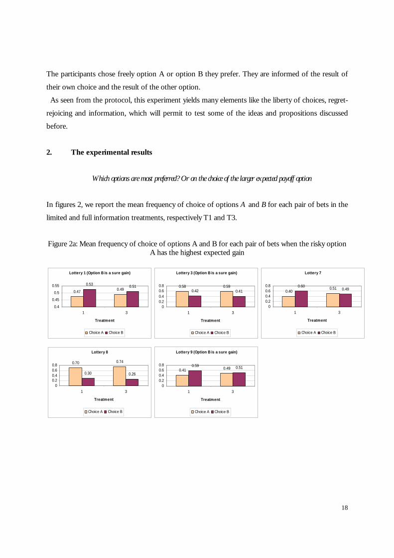
In figures 2, we report the mean frequency of choice of options A and B for each pair of bets in the
limited and full information treatments, respectively T1 and T3.
Figure 2a: Mean frequency of choice of options A and B for each pair of bets when the risky option A has the highest expected gain
Lottery 1 (Option B is a sure gain)
0.47 0.490.53 0.51
0.4
0.45
0.5
0.55
1 3
Treatment
Choice A Choice B
Lottery 3 (Option B is a sure gain)
0.58 0.590.42 0.41
00.20.40.60.8
1 3
Treatment
Choice A Choice B
Lottery 7
0.400.510.60
0.49
00.20.40.60.8
1 3
Treatment
Choice A Choice B
Lottery 8
0.70 0.74
0.30 0.26
00.20.40.60.8
1 3
Treatment
Choice A Choice B
Lottery 9 (Option B is a sure gain)
0.41 0.490.59 0.51
00.20.40.60.8
1 3
Treatment
Choice A Choice B
19
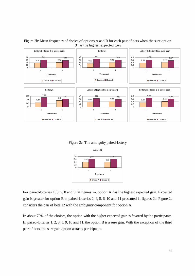
Figure 2b: Mean frequency of choice of options A and B for each pair of bets when the sure option
B has the highest expected gain
Figure 2c: The ambiguity paired-lottery
Lottery 12
0.40 0.390.60 0.61
00.20.40.60.8
1 3
Treatment
Choice A Choice B
For paired-lotteries 1, 3, 7, 8 and 9, in figures 2a, option A has the highest expected gain. Expected
gain is greater for option B in paired-lotteries 2, 4, 5, 6, 10 and 11 presented in figures 2b. Figure 2c
considers the pair of bets 12 with the ambiguity component for option A.
In about 70% of the choices, the option with the higher expected gain is favored by the participants.
In paired-lotteries 1, 2, 3, 5, 9, 10 and 11, the option B is a sure gain. With the exception of the third
pair of bets, the sure gain option attracts participants.
Lottery 2 (Option B is a sure gain)
0.38 0.420.62 0.58
00.20.40.60.8
1 3
Treatment
Choice A Choice B
Lottery 4
0.33 0.410.67 0.59
00.20.40.60.8
1 3
Treatment
Choice A Choice B
Lottery 5 (Option B is a sure gain)
0.38 0.430.62 0.57
00.20.40.60.8
1 3
Treatment
Choice A Choice B
Lottery 6
0.470.49
0.530.51
0.4
0.45
0.5
0.55
1 3
Treatment
Choice A Choice B
Lottery 10 (Option B is a sure gain)
0.37 0.430.63 0.57
00.20.40.60.8
1 3
Treatment
Choice A Choice B
Lottery 11 (Option B is a sure gain)
0.34 0.40
0.66 0.60
00.20.40.60.8
1 3
Treatment
Choice A Choice B

20
The result for the paired-lottery 3 is interesting since it contradicts Kahneman and Tversky’s (1979)
result in their seminal work with a near equivalent paired lottery (4000: 8/10. 0:2/10 ; 3000: 10/10)
and where the sure gain was favored by 80% of participants although the gamble has a higher
expected value. A potential explanation for this difference lays with the information gathered on
experienced probabilities when participants play 120 times in our experiment! They get eventually
convince that option A is an interesting bet given the odds.
For paired-lotteries 4 and 8 where 1 2( , ) ( , )A y p and B y p ε= = + with
10,0,021 <<<>>> pyy ε , the expected utility model choice applies.
For the paired-lottery 12 with the ambiguity component for option A, the option B with a 50%
chance to win 6000 ECUS or nothing is clearly preferred.
Some graphics indicate differences in choices between T1 and T3, for some paired-lotteries, with a
reversal in mean choices for the paired-lottery 7. In the treatment with the limited information, T1,
option B dominates despite the higher expected value of option A. But when the full information is
revealed, T3, both options are almost equally chosen. It may well be the case again that by playing
many times the same paired-lottery and all paired-lotteries in general, a probability of 60% appears a
relatively a good odd to gamble on the riskiest option.
Figure 3 shows how information might affect the dynamics of choices. In general, option A is
preferred to option B with the treatment with full information, T3. In the first period, for all paired-
lotteries confounded (excluding paired-lottery12), there is not much difference between the
treatments in the proportion of choice of option A. But over the number of plays with the
information cumulating in the full information treatment, participants in that treatment appear to
choice more frequently the more risky choice A relatively to those involved with the limited
information treatment.

21
Figure 3: Proportion of choice A per treatment per play (without lottery 12).
0
0.1
0.2
0.3
0.4
0.5
0.6
1 2 3 4 5 6 7 8 9 10
Play
Treatment 1 Treatment 3
In table 2, we report the results of a random effect probit model on the choice or option A, the
more risky choice.

22
Table 2: Determinants of choosing option A (Random-effects probits)
Limited information (T1) Full information (T3)
Coefficient. p>z Coefficient z
A is the highest expected payoff
0.1874 (0.1085)
0.084 0.2814 (0.0984)
0.004
B is the highest expected payoff
-0.2045 (0.1085)
0.059 -0793 (0.0982)
0.419
B is a sure gain -0.1348 (0.4153)
0.001 -0.1780 (0.0421)
0.000
Paired-lottery12 0.00101 (0.0854)
0.991 -0.2009 (0.0861)
0.020
Play number -0.0095 (0.0067)
0.154
0.00268 (0.0068)
0.692
Period -.000338 (0.0095)
0.594 -0.000233 (0.00064)
0.715
Rho 0.2493 (0.04455)
0.000 0.1786 (0.0369)
0.000
log likelihood -2991. 76 -2908.97
# of observation 4 920 4560
The regression results confirm the attractiveness of the sure gain option in the limited information
treatment. It has also play a role in the full information treatment along with the situation when
option A offers the highest expected payoff. As participants play a number of times the paired-
lottery, the probability of choosing option A declines for the limited treatment but remains constant
in the full information treatment. However, the coefficients of this variable and of the period
variable are statistically insignificant.
What is satisfaction?
We have argued in previous sections that reported satisfaction is not an ex ante measure of the
utility, but measures an ex post latent preference for the choice made. In other words, it is an
23
experienced utility or related to ex post utility. After the outcome of your choice, you are either
happy with your choice or not.
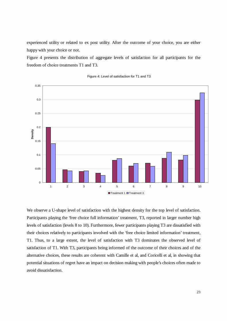
Figure 4 presents the distribution of aggregate levels of satisfaction for all participants for the
freedom of choice treatments T1 and T3.
Figure 4: Level of satisfaction for T1 and T3
0
0.05
0.1
0.15
0.2
0.25
0.3
0.35
1 2 3 4 5 6 7 8 9 10
Den
sity
Treatment 1 Treatment 3
We observe a U-shape level of satisfaction with the highest density for the top level of satisfaction.
Participants playing the ‘free choice full information’ treatment, T3, reported in larger number high
levels of satisfaction (levels 8 to 10). Furthermore, fewer participants playing T3 are dissatisfied with
their choices relatively to participants involved with the ‘free choice limited information’ treatment,
T1. Thus, to a large extent, the level of satisfaction with T3 dominates the observed level of
satisfaction of T1. With T3, participants being informed of the outcome of their choices and of the
alternative choices, these results are coherent with Camille et al, and Coricelli et al, in showing that
potential situations of regret have an impact on decision making with people’s choices often made to
avoid dissatisfaction.

24
To explore the determinants of satisfaction, we report in table 3, the results of a panel probit on our
measure of reported satisfaction regress on variables constructed to reflect our theoretical arguments
and those of others. To simplify the analysis in panel, we have run a binary regression with a positive
level of satisfaction defined set to 1 if the reported level is 8 or above, and 0 otherwise.
The following independent variables were constructed:
Expected payoff of the chosen option. Note that for lottery 12, in the ambiguity option, we
assume that the participant considers an equal probability of 50% for both outcomes.
Expected payoff of the chosen option*lottery12. A crossed variable.
If satisfaction is utility, we expect positive statistically significant coefficient affecting the expected
pay off variable since it represents a good approximation of expected utility.
Risk averse participant: The number of times that the participant has chosen the sure option when
available.
This is an idiosyncratic measure of risk attitude of participants, a control variable.
Number of gains with the alternative choice prior to decision: This variable is constructed for
all the 12 lotteries for T3. For T1, it is available only when the participant has chosen the option A
of a lottery where the option B is a sure gain; it is set to 0 otherwise. Having realised what could
have happened, it is a measure of regret and we expect a negative sign coefficient.
Gap between payoffs: The realised payoff minus the alternative payoff. Again this variable is
constructed for all the 12 lotteries for T3. For T1, it is available only when the participant has
chosen the option A of a lottery where the option B is a sure gain; it is set to 0 otherwise. A negative
value is a form of regret, while a positive value yields matter for rejoice. Thus the expected
coefficient is positive.
Payoff when the winning choice is from a risky option and its square.
Payoff when the winning choice is a sure outcome and its square.
These variables with a positive coefficient simply stress that winning more increases happiness. We
expect a negative sign on the square of these variables following our proposition that the sensitivity
of satisfaction diminishes with the size of the gain (see proposition 2).

25
Lottery 12: A binary dummy variable.
Table 3: Determinants of satisfaction with free choices
(Random-effects probits)
Coef. P>z
Expected payoff of the choice option -0.0000585 (0.0000317)
0.065
Expected payoff of the choice option*lottery12
-0000938 (0.0000305)
0.002
Risk averse participant
0.006578 (0.00777)
0.397
# of wins with alternative choice prior to decision
-0.02410 (0.01048)
0.021
Gap between payoffs 0.000253 (0.0000153)
0.000
Payoff from a winning risky option 0.001212 (0.0000346)
0.000
Payoff f.w.r.o. squared -1.24e-07 (5.04e-09)
0.000
Payoff from a winning sure choice 0.0001780 (0.0000726)
0.000
Payoff f.w.s.c. squared -3.35e-07 (2.35e-08)
0.000
Constant -1.5778 (0.4470)
0.000
Rho 0.5745 (0.04139)
Log likelihood: -3229.68; Prob > chi2 = 0.0000. Likelihood-ratio test of rho = 0: chibar2 (01) = 2644; Prob >= chibar2 = 0.000. Number of observations: 9 840.
Table 3 indicates that the variable ‘Expected payoff of the chosen lottery’ is statistically insignificant
coefficients in explaining satisfaction. We therefore reject the hypothesis that satisfaction is a
measure of ex ante utility. Furthermore, the negative coefficients on expected payoff variables are
puzzling.

26
The hypothesis of a constant utility, ex ante or ex post, is rejected by the data, considering the strong
effect of the “# of wins with alternative choices prior to decision” variable. In other words, regret
and information from the past explain satisfaction but, not utility. The regret-rejoice variable, ‘gap
between payoffs’ confirm that bad and good surprises explain satisfaction, and again is not coherent
with the hypothesis that satisfaction measures ex ante utility. Bigger winning payoffs increase
satisfaction, a result coherent with the hypothesis that satisfaction is experienced utility or related to
ex post utility. The negative sign on the squared variables confirm that the sensitivity of satisfaction
diminishes with the size of the gain.
In view of those results, satisfaction is not a measure of ex ante utility but a measure of an ex post
latent preference for the choice made.
If your are satisfy, you repeat your choice
If the theory of expected utility explains the participants’ choices, no change should occur. However
on average, we have observed that in 27.5% of cases a different decision is made.
Further evidence supporting that satisfaction is an emotion leading to a decision, is reported in table
4 on the effect on the probability that a participant will change his decision when he is satisfied with
his previous choice. We have argued that reporting one’ satisfaction is the judgment that one would
wish to repeat one’s past experience if one could choose again.
Table 4: Determinants of the probability of changing option (Random-effects probit)
Coef. P>z
Past satisfaction* -0.0201 (0.00486)
0.000
Risk adverse participant -0.00446 (0.00444)
0.315
Constant -0.40559 (0.18412)
0.028
Rho 0.25269 (0.03385)
*Scale 1 to 10.
Log likelihood: -4525.3095; Prob > chi2 = 0.0001. Likelihood-ratio test of rho=0: chibar2 (01) = 936.47; Prob >= chibar2 = 0.000. Number of observations: 8 532.
27
The results of table 4 show that if you are satisfied with your past choice, the lower the probability
you will change it. Note that 50% of people report a level of satisfaction greater than eight on a scale
of 1 to 10. At the lowest level of reported satisfaction, the probability of changing his choice is
30.24% and drops to 23.42% if reported satisfaction from the previous choice is at level 10.
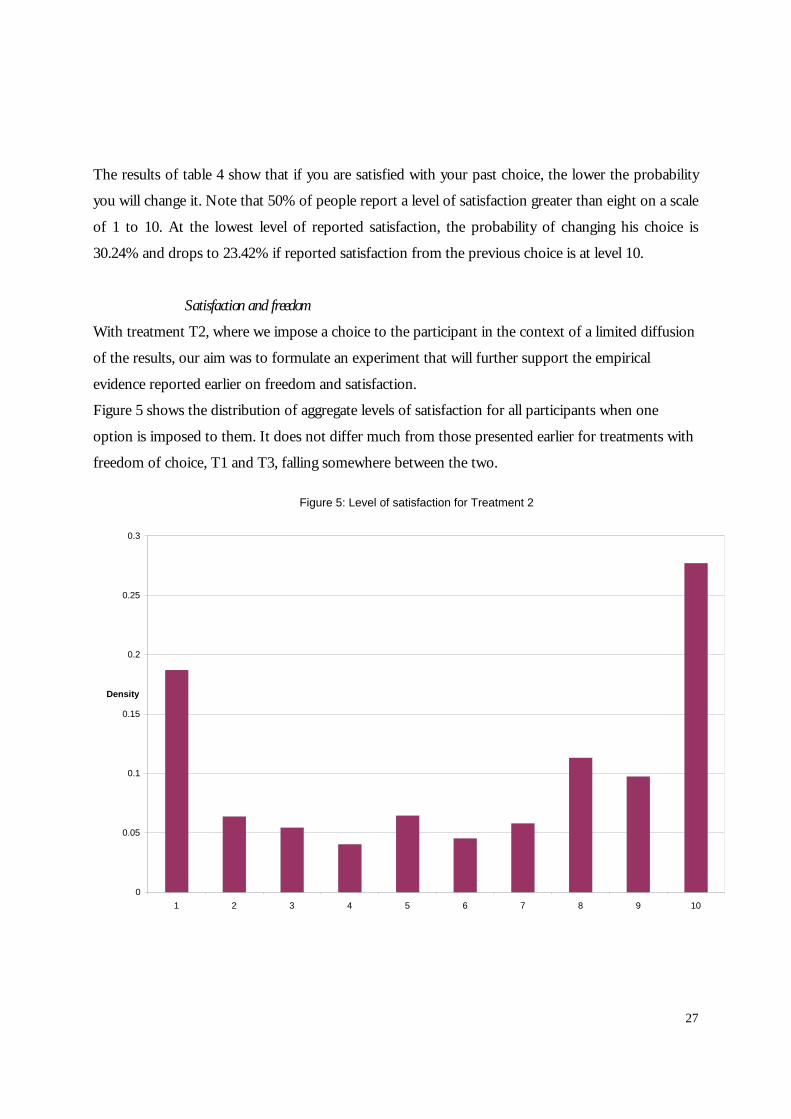
Satisfaction and freedom
With treatment T2, where we impose a choice to the participant in the context of a limited diffusion
of the results, our aim was to formulate an experiment that will further support the empirical
evidence reported earlier on freedom and satisfaction.
Figure 5 shows the distribution of aggregate levels of satisfaction for all participants when one
option is imposed to them. It does not differ much from those presented earlier for treatments with
freedom of choice, T1 and T3, falling somewhere between the two.
Figure 5: Level of satisfaction for Treatment 2
0
0.05
0.1
0.15
0.2
0.25
0.3
1 2 3 4 5 6 7 8 9 10
Density
28
One difficulty with our experiment is that the treatments were not played sequentially, denying to
participants an alternative to the game they played. They might not have totally felt their constrained
choice as they could not have perceived that other participants have played with a free choice in
treatments T1 or T3. If will also have been interesting to have a treatment with no choice but with
full information displayed to the participants. There is one situation however, where the constraint
might have been felt stronger is when the participant did not win.
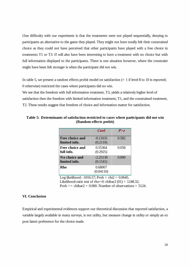
In table 5, we present a random effects probit model on satisfaction (= 1 if level 8 to 10 is reported;
0 otherwise) restricted the cases where participants did no win.
We see that the freedom with full information treatment, T3, yields a relatively higher level of
satisfaction then the freedom with limited information treatment, T1, and the constrained treatment,
T2. These results suggest that freedom of choice and information matter for satisfaction.
Table 5: Determinants of satisfaction restricted to cases where participants did not win (Random-effects probit)
Coef. P>z
Free choice and limited info.
-0.11631 (0.2110)
0.582
Free choice and full info.
0.55364 (0.2925)
0.058
No choice and limited info.
-2.25130 (0.1541)
0.000
Rho 0.68007 (0.04110)
Log likelihood: -1016.57; Prob > chi2 = 0.0645. Likelihood-ratio test of rho=0: chibar2 (01) = 1248.32; Prob >= chibar2 = 0.000. Number of observations = 5124.
VI. Conclusion
Empirical and experimental evidences support our theoretical discussion that reported satisfaction, a
variable largely available in many surveys, is not utility, but measure change in utility or simply an ex
post latent preference for the choice made.

29
This distinction between satisfaction and utility has the major implication that the reference-
dependence of satisfaction need not contaminate utility analysis. It is important to recognize that so
much puzzling behavior, which has long marked a dividing line between economics and other
disciplines, like sociology and psychology, appear to be wholly consistent with standard utility
analysis once the distinction has been recognized.
The variable satisfaction largely presents in survey data has led to many interesting studies by
economists and others to explain a whole set of decisions by individuals. We expect that using this
variable in an experimental context will also be useful for research on human behavior. More work is
needed, however, to cope with this challenge.
Appendix: The 12 paired-lottery choices
# Option A Option B Expected payoff difference
1 2/10 of 4500, 8/10 of 0 10/10 of 800 100
2 8/10 of 3000, 2/10 of 0 10/10 of 2500 -100
3 8/10 of 4500, 2/10 of 0 10/10 of 3400 200
4 2/10 of 3000, 8/10 of 0 3/10 of 2500, 7/10 of 0 -150
5 2/10 of 4000, 8/10 of 0 10/10 of 900 -100
6 7/10 of 1100, 3/10 of 0 9/10 of 900, 1/10 of 0 -40
7 6/10 of 5000, 4/10 of 0 9/10 of 3000, 1/10 of 0 300
8 2/10 of 6000, 8/10 of 0 3/10 of 3000, 7/10 of 0 300
9 1/10 of 8000, 9/10 of 0 10/10 of 700 100
10 6/10 of 5000, 4/10 of 0 10/10 of 3200 -200
11 1/10 of 10000, 9/10 of 0 10/10 of 1100 -100
12 ? of 6000, ? of 0 5/10 of 6000, 5/10 of 0 ----
30
REFERENCES Argyle, M. (1999), “Causes and Correlates of Happiness”, in Well-being: The Foundations of Hedonic Psychology, Kahneman, D., E. Diener, and N. Schwartz (eds.), New York: Russell Sage, 353-373. Aronson, E. (1992), The Social Animal, New York: W.H. Freeman and Co., 6th edition (first edition 1972). Becker, G.S. and C.B. Mulligan (1997), “The Endogenous Determination of Time Preference”, Quarterly Journal of Economics 112, 729-758. Bentham, J. (1789) An Introduction to the Principles of morals and Legislation. Boudon, R. (1977), Effets Pervers et Ordre Social, Paris:Presses Universitaires de France. Borjas, G. (1979), “Job Satisfaction, Wages and Unions”, Journal of Human Resources 14, 21-40. Campbell, A. (1981), The Sense of Well-Being in America: Recent Patterns and Trends, New-York: Mac Graw Hill. Brickman, P. and D.T. Campbell (1971), “Hedonic Relativism and Planning the Good Society”, in Adaptation-level Theory: A Symposium, M.H. Apley (ed.), New York: Academic Press. Brickman, P., D. Coates, and R. Janoff-Bulman (1978), “Lottery Winners and Accident Victims: Is Happiness Relative?”, Journal of Personality and Social Psychology 37, 917-927. Camille N, G. Coricelli, J Sallet, P Pradat-Diehl, J.R. Duhamel. A. Sirigu, “The Involvment of the Orbitofrontal Cortex in the Experience of Regret”, Science, 2004, 1167-1170. Charness G., et B. Grosskopf, “Relative payoffs and happiness: An experimental study”, Journal of Economic Behavior and Organisation, 45, 2001, 301-328. Clark, A.E. and A.J. Oswald (1994), “Unhappiness and Unemployment”, Economic Journal 104, 648-659. Clark, A.E. and A.J. Oswald (1996), “Satisfaction and Comparison Income”, Journal of Public Economics 61, 359-381. Clark, A.E., A.J. Oswald, and P.B. Warr (1996), “Is Job Satisfaction U-shaped in Age?”, Journal of Occupational and Organizational Psychology 69, 57-81. Coricelli G., H.D. Critchley, M. Joffily, J.P. O’Doherty, A Sirigu et R.J. Dolan, “Regret ans its avoidance: A neuroimaging study of choice behavior”, Nature Neuroscience, 8 (9), 2005, 1255-1261. Damasio, A.R. (1994), Descartes’ Error, New York: Avon. Diener, E., M. Diener and C. Diener (1995), “Factors Predicting the Subjective Well-Being of Nations”, Journal of Perssonality and Social Psychology 69, 851-864. Diener, E. and C. Diener (1996), “Most People are Happy”, Psychological Science 7, 181-185. Diener, E. and R. Lucas (1999), “Personality and Subjective Well-Being”, in Well-Being: The Foundations of Hedonic Psychology, D. Kahneman, E. Diener, and N. Schwartz (eds.), New York: Russell Sage, 213-229. Diener, E. and E. Suh (1997), “Measuring Quality of Life: Economic, Social, and Subjective Indicators”, Social Indicators Research 40, 189-216. Diener, E., E.M. Suh, R.E. Lucas and H.L. Smith (1999), “Subjective Well-Being: Three Decades of Progress”, Psychological Bulletin 125, 276-303.
31
Easterlin, R.A. (1974), “Does Economic Growth Improve the Human Lot? Some Empirical Evidence”, in Nations and Households in Economic Growth, P.A. David and M.W. Reder (eds.), New York: Academic Press, 89-125. Easterlin, R.A. (1995), “Will Raising the Incomes of All Increase the Happiness of All?”, Journal of Economic Behavior and Organization 27, 35-47. Festinger, L. (1957), A Theory of Cognitive Dissonance, Stanford, Cal. : Stanford University Press. Frederick, S. and G. Loewenstein (1999), “Hedonic Adaptation”, in Well-Being: The Foundations of Hedonic Psychology, D. Kahneman, E. Diener, and N. Schwartz (eds.), New York: Russell Sage, 302-329. Freeman, R.B. (1978), “Job Satisfaction as an Economic Variable”, American Economic Review: Papers and Proceedings 68, 135-141. Frey, B.S. and A. Stutzer (2000), “Happiness, Economy and Institutions”, Economic Journal 110, 918-938. Gerlach, K. and G. Stephan (1996), “A Paper on Unhappiness and Unemployment in Germany”, Economics Letters 52, 325-330. Hamermesh, D.S. (1977), “Economic Aspects of Job Satisfaction”, in Essays in Labor Market Analysis, O.C. Ashenfelter and W.E. Oates (eds.), New York: John Wiley & Sons, 53-72. Kahneman, D. and A. Tversky (1979), ¨Prospect Theory¨, Econometrica, 47(2), 263-291. Kahneman, D. (1999), “Objective Happiness”, in Well-Being: The Foundations of Hedonic Psychology, D. Kahneman, E. Diener, and N. Schwartz (eds.), New York: Russell Sage, 3-25. Kahneman, D., P.P. Wakker and R. Sarin (1997), “Back to Bentham? Explorations of Experienced Utility”, Quarterly Journal of Economics 112, 325-405. Lévy-Garboua, L. and C. Montmarquette (2004), “Reported Job Satisfaction: What Does it Mean?”, Journal of Socio-Economics, 33(2), 135-151. Lévy-Garboua, L. and C. Montmarquette (1996), “A Microeconometric Study of Theatre Demand”, Journal of Cultural Economics 20, 25-50. Lévy-Garboua L,C. Montmarquette and V. Simonnet, “Job Satisfaction and Quits”, Labour Economics, 2007, 14(2), 251-268. Michalos, A.C. (1980), “Satisfaction and Happiness ”, Social Indicators Research 8, 385-422. Oswald, A.J. (1997), “Happiness and Economic Performance”, Economic Journal 107, 1815-1831. Rabin, M. (1998), “Psychology and Economics”, Journal of Economic Literature 36, 11-46. Redelmeier, D. and D. Kahneman (1996), “Patients’ Memories of Painful Medical Treatments: Real-time and Retrospective Evaluations of Two Minimally Invasive Procedures”, Pain 116, 3-8. Sen, A. (1999), Development as Freedom, New York: Anchor Books, Random House. Sousa-Poza, A. and A.A Sousa-Poza (2000), “Well-being at Work: A Cross-national Analysis of the Levels and Determinants of Job Satisfaction”, Journal of Socio-Economics 29, 517-538. Tversky, A. and D. Kahneman (1991), “Loss Aversion in Riskless Choice: A Reference Dependent Model”, Quarterly Journal of Economics 106, 1031-1061. Veenhoven, R. (1996), “Developments in Satisfaction-Research”, Social Indicators Research 37, 1-46.

32
Veehoven, R. (2000), “Freedom and Happiness: A Comparative Study in Forty-four Nations in the Early 1990s”, in Culture and Subjective Well-Being, E. Diener and E.M. Suh (eds.), Cambridge, Mass.: MIT Press, 257-288. Winkelmann, L. and R. Winkelmann (1998), “Why are the Unemployed so Unhappy? Evidence from Panel Data”, Economica 65, 1-15. Zajonc, R.B. (1980) “Feeling and Thinking: Preferences Need No Inferences”, American Psychologist 35, 151-175.
33
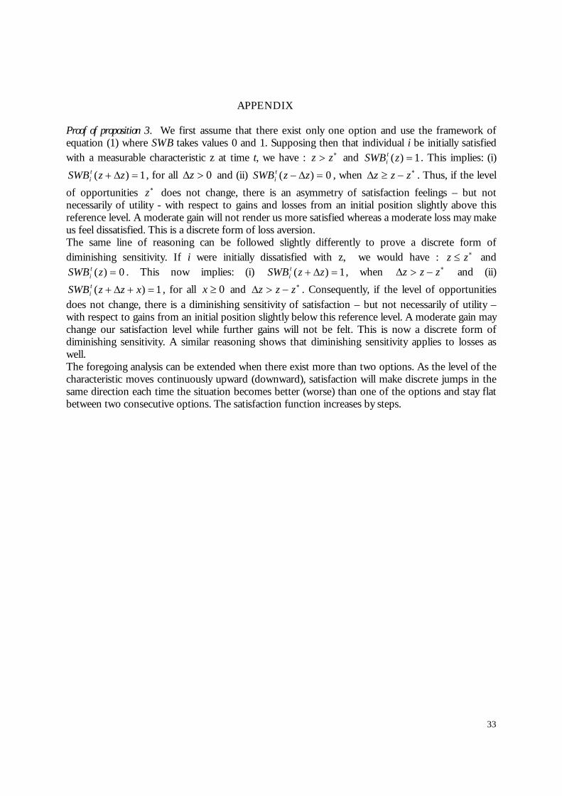
APPENDIX Proof of proposition 3. We first assume that there exist only one option and use the framework of equation (1) where SWB takes values 0 and 1. Supposing then that individual i be initially satisfied with a measurable characteristic z at time t, we have : ∗> zz and 1)( =zSWBt
i . This implies: (i) 1)( =∆+ zzSWBt
i , for all 0>∆z and (ii) 0)( =∆− zzSWB ti , when ∗−≥∆ zzz . Thus, if the level
of opportunities ∗z does not change, there is an asymmetry of satisfaction feelings – but not necessarily of utility - with respect to gains and losses from an initial position slightly above this reference level. A moderate gain will not render us more satisfied whereas a moderate loss may make us feel dissatisfied. This is a discrete form of loss aversion. The same line of reasoning can be followed slightly differently to prove a discrete form of diminishing sensitivity. If i were initially dissatisfied with z, we would have : ∗≤ zz and
0)( =zSWB ti . This now implies: (i) 1)( =∆+ zzSWB t
i , when ∗−>∆ zzz and (ii) 1)( =+∆+ xzzSWB t
i , for all 0≥x and ∗−>∆ zzz . Consequently, if the level of opportunities does not change, there is a diminishing sensitivity of satisfaction – but not necessarily of utility – with respect to gains from an initial position slightly below this reference level. A moderate gain may change our satisfaction level while further gains will not be felt. This is now a discrete form of diminishing sensitivity. A similar reasoning shows that diminishing sensitivity applies to losses as well. The foregoing analysis can be extended when there exist more than two options. As the level of the characteristic moves continuously upward (downward), satisfaction will make discrete jumps in the same direction each time the situation becomes better (worse) than one of the options and stay flat between two consecutive options. The satisfaction function increases by steps.