A Theory of Dumping and Anti-dumping1

Phillip McCalman2 Frank Stahler3 Gerald Willmann4

Preliminary version of February 2009

1The usual disclaimer applies: all errors are ours.2Department of Economics, University of California, Santa Cruz CA 95064, USA, email: mc-

calman@ucsc.edu3Department of Economics and CESifo, University of Otago, PO Box 56, Dunedin 9001, New

Zealand, email: fstaehler@business.otago.ac.nz4Department of Economics, Katholieke Universiteit Leuven, Naamsestraat 69, 3000 Leuven,

Belgium, email: gerald.willmann@econ.kuleuven.be

Abstract

This paper develops an efficiency theory of antidumping policy. We model the competition

for a domestic market between one domestic and one foreign firm as a pricing game under

incomplete information about production costs, where an asymmetry in distribution of

costs arises due to trade costs. We show that the foreign firm prices more aggressively. The

resulting probability of an inefficient allocation justifies the use of anti-dumping policy on

efficiency grounds. Seeking to maximize global welfare, conditional ex-post trade policy

avoids the potential inefficiency. Anti-dumping policy conducted by national governments,

on the other hand, leads to excessive use due to rent shifting motives. The inefficiency

probability of this policy is larger (smaller) for low (high) trade costs compared to the

laissez faire.

Keywords: Dumping, Conditional Trade Policy, Auction with Asymmetric Valuations.

JEL Classifications: F12, F13, D44.

1 Introduction

Anti-dumping policy occupies a dubious niche within the trade policy literature; not only

is it seen as a policy to counter a rarely observed phenomena - and therefore have only the

thinnest of possible efficiency rationales - but when they are applied, anti-dumping duties

are seen as gratuitous in size - with duties of the order of 100% not unusual.1 With its

ability to raise the ire of every economist that encounters it, it is hardly surprising that

there is a voluminous literature documenting the shortcomings of anti-dumping policy

from both a theoretical and empirical perspective.2 Consequently, it would seem difficult

to defend the operation of a policy so bereft of credibility. However, that is exactly the goal

of this paper - to develop an efficiency rationale for a policy of anti-dumping. In doing so

we provide a perspective on why it operates in the way that it does and in particular what

is at the heart of its failure to achieve any desirable outcomes. Moreover, our analysis also

provides important insights into both the rise in the frequency of anti-dumping cases (and

whether this phenomena is likely to be sustained) and what reforms would rehabilitate the

concept of contingent protection and legitimize the use of anti-dumping duties.

Our point of departure is to move the rationale for the policy away from the usual mo-

tivation of predation toward a broader and more relevant concept of allocative efficiency.3

Therefore we focus on the question of who should be producing what and whether trade

policy, in the form of anti-dumping duties, has a role to play in improving efficiency. If

a policy-maker has complete information about the relevant costs, then determining the

optimal allocation of resources is straight forward and the only real concern is one of policy

failure. This is the element - policy failure - that the previous literature has focused on

and sought to stress. If the policy-maker is incompletely informed about the cost structure,

then both the mechanics of competition become more involved and the criteria for deter-

mining government intervention becomes less transparent. In this setting it is possible to

have a market failure that cannot be adequately addressed by government intervention. It

is this environment of asymmetric information in which we couch our analysis.

1See Bown (2007).2See Blonigen and Prusa (2004).3Our focus on price discrimination is reminiscent of Brander and Krugman (1983). However, while

dumping occurs in their framework it is not the focus of their analysis. As discussed below we adopt amarket structure that emphasizes the resource allocation issues associated with dumping and provides aclear policy benchmark.

1

More specifically we develop a model of international competition where neither firm is

reliably informed of the others cost structure. To sharpen the implications of competition,

we assume that the firms produce a homogeneous product and compete in prices; generat-

ing a winner-take-all scenario. Under complete information this set-up achieves allocative

efficiency. Allocative efficiency is also achieved under the assumption of symmetry when

firms are incompletely informed (that is, both firms are assumed to take cost draws from

the same probability distribution). The virtue of this set-up is that under either complete

information or in a symmetric incomplete information setting there is no market failure

and therefore no need for government intervention. This provides us with a clear and un-

ambiguous benchmark. However, as a model of international competition it is lacking a

critical feature - transport costs. The introduction of transport costs implies that the firms

are no longer symmetric. This small, but realistic, change has profound implications for

the allocation of resources: despite the winner-take-all nature of competition the higher

cost firm can ultimately be the sole supplier in the market. This market failure has a clear

source; since the foreign firm is at a disadvantage due to transport costs it will price more

aggressively than the domestic firm. Consequently, when both firms have the same cost

draws (inclusive of transport costs), the foreign firm will quote a strictly lower price. This

implies two things. First, in the neighborhood of these cost draws it is possible to iden-

tify outcomes where the higher cost foreign firm serves the domestic market; an inefficient

allocation of resources. Second, the foreign firm is dumping; the foreign firm prices more

aggressive abroad than in their local market.4

Given this market failure the question we address is whether anti-dumping policy can

achieve an efficient allocation of resources.5 This requires that we determine two things.

First, can a government infer which firm is the lower cost producer for any given set of

cost draws? If this cannot be done then it is clear that government intervention cannot

achieve the first best outcome. Second, even if a government can determine which firm is

the lowest cost producer in a laissez fair system, and therefore determine when to intervene,

4Dumped imports are defined under U.S. law to be foreign products exported to the U.S. market atprices below ”fair value,” that is, either below the prices of comparable products for sale in the domesticmarket of the exporting country or below costs of production.

5A number of other papers have considered an environment of asymmetric information: Miyagiwa andOhno (2007), Matschke and Schottner (2008) and Kolev and Prusa1 (2002). However, these papers areconcerned with the implications of anti-dumping policy on firm behavior (output, prices and profits) anddon’t investigate whether anti-dumping duties can achieve a first best outcome.

2

does the announcement of a mechanism for intervention still enable such an inference to be

drawn? That is, the announcement of a policy framework is likely to change the behavior

of the firms which can undermine the ability of the government to determine whether a

mis-allocation of resources has occurred.6 We show that it is possible for a government to

infer cost under a laissez fair system and also design an anti-dumping policy that would

preserve this inferential ability; that is, a first best outcome can be achieved. However, the

ability to achieve the first best doesn’t necessarily mean that it will be implemented. Two

major obstacles are identified. First, a global institution with the goal of maximizing global

welfare could implement a first best policy. However, the distributional implications mean

that it is unlikely to offer unambiguous gains to both countries and therefore maybe vetoed

(though in a symmetric setting the institution would not be vetoed). Nevertheless, if such

an institution existed, there would be no dumping in equilibrium. Second, if the national

governments were to implement anti-dumping policy, they also would have the capacity to

infer which firm had the lowest costs. However, national governments would not have an

incentive to implement the first best outcome. Instead they would exploit the rent shifting

aspect of anti-dumping duties and over use such a policy. As a consequence dumping would

persist in equilibrium, but it is not necessarily the largest source of inefficiency compared

to market failure. This last point raises the issue of the relative cost of market versus

government failure. In relation to this issue, we show that dumping is not likely to occur

when trade barriers are either very high or very low. This has the implication that the very

success of the WTO process in lowering trade barriers (along with technological advanced

that have lowered transport costs) has contributed to the stunning increase in the number

of anti-dumping cases. However, it also suggests that pursuing further trade liberalization

will reverse this trend and diminish the number of anti-dumping cases.

The remainder of the paper is structured as follows: In Section 2 we setup the model,

solve for the price functions, and show that inefficiency can arise. Section 3 analyzes the

globally optimal anti-dumping policy, and Section 4 analyses what a national government

seeking to maximize national welfare would do. Section 5 offers concluding remarks.

6In a complete information setting, Staiger and Wolak (1992) and Anderson (1992) make the pointthat the mere existence of anti-dumping policy will alter firms behavior.

3

2 The model

We consider a domestic commodity market in which consumers have unit demands. Their

maximum willingness to pay is one, and without loss of generality, we normalize the size

of consumers to one. There are potentially two rival firms in this market, a domestic firm,

labelled 1, and a foreign firm, labelled 2. Both firms compete against each other by prices,

but their production costs c1 and c2 are private information. Furthermore, the foreign firm

has to carry an additional per unit trade cost of size t which is common knowledge. Without

any intervention, consumers will all buy from firm i if pi < pj. As we will see below, there

will never be a case for a policy intervention if the domestic firm wins. However, if the

foreign firm wins, an import tariff τ may be imposed such that p2+τ > p1 although p2 < p1.

p1 ≥ c1 is the price which the domestic firm is allowed to charge after the intervention.

Before it potentially comes to competition between the two firms, the foreign firm has

to decide whether it would like to enter the domestic market or not. If it wants to, it has to

make an investment of size g which can be observed by the domestic firm. This investment

should be of small size in our setting, for example the search cost of finding a wholesaler

and/or retailer. In any case, the entry decision potentially signals a certain productivity

range of the foreign firm to the domestic firm which will update its beliefs accordingly.

Table 1 gives the sequence of decisions of the game, which we solve in the usual backward

induction fashion. Obviously, if the foreign firm does not enter the market, the domestic

firm is a monopolist and will set p1 equal to one.

In case of entry by the foreign firm, it is obvious that it will never be optimal for any

firm to charge a price strictly larger than one as this will make sure that it will not be

successful on the market. Assume that the optimal pricing functions pi(ci) are monotonic

and strictly increasing in costs. In this case, inverse price functions exist which are also

monotonic and strictly increasing with prices, and we denote these inverse price functions

by φi(pi). Let F1(c1) denote the distribution of costs from which the domestic firm draws

its cost realization. Similarly, F2(c2) will denote the distribution of costs from which those

foreign firm draw their cost realization which will enter the market. Hence, F2(c2) is based

on a Bayesian update from the basic distribution G2(c2) which is done by the domestic

firm as to determine with which types of rivals it has to deal with. We use this updated

distribution as it will decide on the success of the domestic firm. If the domestic firm sets

its price equal to p1 and the foreign firm employs the price function p2(c2) (or, equivalently,

4

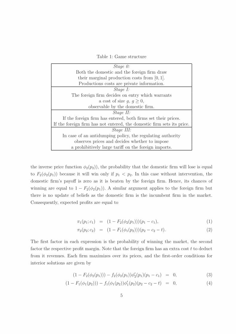
Table 1: Game structure

Stage 0:Both the domestic and the foreign firm drawtheir marginal production costs from [0, 1].Productions costs are private information.

Stage I:The foreign firm decides on entry which warrants

a cost of size g, g ≥ 0,observable by the domestic firm.

Stage II:If the foreign firm has entered, both firms set their prices.

If the foreign firm has not entered, the domestic firm sets its price.Stage III:

In case of an antidumping policy, the regulating authorityobserves prices and decides whether to impose

a prohibitively large tariff on the foreign imports.

the inverse price function φ2(p2)), the probability that the domestic firm will lose is equal

to F2(φ2(p1)) because it will win only if p1 < p2. In this case without intervention, the

domestic firm’s payoff is zero as it is beaten by the foreign firm. Hence, its chances of

winning are equal to 1 − F2(φ2(p1)). A similar argument applies to the foreign firm but

there is no update of beliefs as the domestic firm is the incumbent firm in the market.

Consequently, expected profits are equal to

π1(p1; c1) = (1 − F2(φ2(p1)))(p1 − c1), (1)

π2(p2; c2) = (1 − F1(φ1(p2)))(p2 − c2 − t). (2)

The first factor in each expression is the probability of winning the market, the second

factor the respective profit margin. Note that the foreign firm has an extra cost t to deduct

from it revenues. Each firm maximizes over its prices, and the first-order conditions for

interior solutions are given by

(1 − F2(φ2(p1))) − f2(φ2(p1))φ′

2(p1)(p1 − c1) = 0, (3)

(1 − F1(φ1(p2))) − f1(φ1(p2))φ′

1(p2)(p2 − c2 − t) = 0, (4)

5

where f1(c1) = F ′

1(c1)(f2(c1) = F ′

2(c1)) denotes the density function of F1(c1)(F2(c2)). As

for the distribution of costs, we make the following assumption:

Assumption 1 Domestic and foreign costs, ci, are uniformly distributed over the unit

interval, F1(c1) = c1, f1(c1) = 1, G2(c2) = c2 and g2(c2) = 1.

Assumption 1 will allow us to determine closed form solutions for the optimal pricing func-

tions. Furthermore, the update of beliefs is straightforward: If the domestic firm believes

that only these (productive) types will enter for which c2 ≤ γ, it follows that F2(c2) = c2/γ.

Since dumping will occur in markets which can be accessed by foreign firms easily, we make

another assumption:

Assumption 2 The investment cost for entering the market is very small, i.e., g ≃ 0.

Both assumptions now allow us to determine the optimal pricing behavior in the laissez

faire case of no policy intervention.

Lemma 1 If Assumptions 1 and 2 hold and there is no policy intervention, F2(c2) =

1/(1 − t), that is, firm 2 enters if c2 ≤ 1 − t. In case of entry, the equilibrium pricing

functions are given by

p1(c1) = 1 −√

1 + 2(1 − c1)2K1 − 1

2(1 − c1)K1

p2(c2) = 1 −√

1 + 2(1 − [c2 + t])2K2 − 1

2(1 − [c2 + t])K2

, (5)

where

K1 =1

2

t(2 − t)

(1 − t)2≥ 0 and K2 = −K1 ≤ 0.

Proof: See Appendix A.1

Note that our solution includes the special case of symmetry when t = 0. In this case, both

price functions take the form

pi(ci) =1

2+

ci

2.

In what follows, we shall consider cases in which entry occurs; the other case is trivial.

Hence, our analysis is conditional upon entry, and it should be clear that a change in

t does not only imply a variation of firm behavior in case of entry, but changes also the

6

probability of entry. Let us now compare both pricing strategies. For this purpose, we start

by defining aggressiveness. We will consider a firm’s pricing strategy as more aggressive if

it has the larger overall cost (which includes t for the foreign firm) compared to its rival

when charging the same price. In terms of aggressiveness, we have a clear result.

Lemma 2 The foreign firm prices more aggressively that the domestic firm.

Proof: See Appendix A.1

The reason is that the foreign firm wants to make up for its disadvantage in overall costs

due to t as to increase its win probability. Since the foreign firm prices more aggressively,

there is a chance that it offers the lower price even though it has the higher overall cost.

Formally, the outcome is inefficient if p2 < p1 and c2 + t > c1. Appendix A.1 shows that

the probability of an inefficient trade is given by:

1

2+

1

(2 − t) (1 − t)− 1

1 − t. (6)

Differentiating this probability with respect to the trade cost yields:

t2 − 4t + 2

2(t2 − 4t + 4). (7)

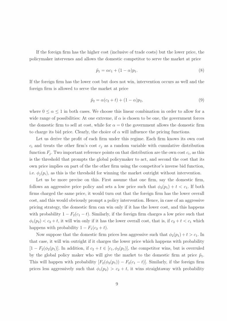
This derivative is positive for low trade costs but becomes negative for higher t. The

resulting non-monotonicity of the probability of inefficiency is displayed in Figure 1. Note

that this also has the interesting interpretation that the phenomena of dumping in our

model is non-monotonic. That is, if trade costs are low, then dumping (or a mis-allocation of

resources) is unlikely to occur because the inefficiency disappears as t goes to zero. Similarly,

if trade costs are very high, then dumping is also unlikely to occur because the foreign

firm is most likely not competitive. However, as trade costs start to fall, the likelihood

of dumping increases. This suggests that the success of the GATT/WTO at liberalizing

trade can possibly explain the increase in dumping. Additionally, further liberalization

might change the situation and lead to less dumping. We return to this discussion in

subsequent sections.

3 Globally Optimal Anti-dumping Policy

We begin our discussion of policy intervention by considering a globally efficient policy.

Such a policy has the objective to avoid the inefficiency and ensure that the lowest cost

7

0.2 0.4 0.6 0.8 1t

0.02

0.04

0.06

0.08

probability

Figure 1: Inefficiency probability in the laissez faire

firm serves the market. However, the global planner cannot directly observe the costs of

the firms, though she can observe the prices that they charge.

A characteristic of the pricing functions that we derive in the previous section is that

they are strictly monotone and therefore invertible. Consequently, a global planner can

deduce from the announced prices what each firm’s costs are, at least in a scenario without

intervention. Allowing the government to intervene changes the nature of the interaction

and may lead to pricing functions that are no longer monotone. This section therefore has

two goals: To determine how the equilibrium pricing functions are altered if the global

planner announces the objective of allocating production to the lowest cost firm. And

second, to check whether the new pricing functions are indeed monotone, because only

then can the policy objective be achieved.

We start by assuming that an equilibrium with strictly monotone pricing functions

exists if the global planner announces her intention to intervene in order to allocate pro-

duction to the lowest cost firm. We interpret this as a global anti-dumping policy. Note

that intervention in our (baseline) model always went against the foreign firm because

the domestic firm never offered the lower price when it has the higher cost. This is not

necessarily true with policy intervention. Furthermore, it should be clear that we do not

need monotonicity across the whole range. For the range c1 ∈ [0, t], a single domestic price

is sufficient as the domestic firm is superior in this range in any case.

8

If the foreign firm has the higher cost (inclusive of trade costs) but the lower price, the

policymaker intervenes and allows the domestic competitor to serve the market at price

p1 = αc1 + (1 − α)p1. (8)

If the foreign firm has the lower cost but does not win, intervention occurs as well and the

foreign firm is allowed to serve the market at price

p2 = α(c2 + t) + (1 − α)p2, (9)

where 0 ≤ α ≤ 1 in both cases. We choose this linear combination in order to allow for a

wide range of possibilities: At one extreme, if α is chosen to be one, the government forces

the domestic firm to sell at cost, while for α = 0 the government allows the domestic firm

to charge its bid price. Clearly, the choice of α will influence the pricing functions.

Let us derive the profit of each firm under this regime. Each firm knows its own cost

ci and treats the other firm’s cost cj as a random variable with cumulative distribution

function Fj . Two important reference points on that distribution are the own cost ci, as this

is the threshold that prompts the global policymaker to act, and second the cost that its

own price implies on part of the the other firm using the competitor’s inverse bid function,

i.e. φj(pi), as this is the threshold for winning the market outright without intervention.

Let us be more precise on this. First assume that one firm, say the domestic firm,

follows an aggressive price policy and sets a low price such that φ2(p1) + t < c1. If both

firms charged the same price, it would turn out that the foreign firm has the lower overall

cost, and this would obviously prompt a policy intervention. Hence, in case of an aggressive

pricing strategy, the domestic firm can win only if it has the lower cost, and this happens

with probability 1 − F2(c1 − t). Similarly, if the foreign firm charges a low price such that

φ1(p2) < c2 + t, it will win only if it has the lower overall cost, that is, if c2 + t < c1 which

happens with probability 1 − F1(c2 + t).

Now suppose that the domestic firm prices less aggressive such that φ2(p1) + t > c1. In

that case, it will win outright if it charges the lower price which happens with probability

[1 − F2(φ2(p1)]. In addition, if c2 + t ∈ [c1, φ2(p1)], the competitor wins, but is overruled

by the global policy maker who will give the market to the domestic firm at price p1.

This will happen with probability [F2(φ2(p1)) − F2(c1 − t)]. Similarly, if the foreign firm

prices less aggressively such that φ1(p2) > c2 + t, it wins straightaway with probability

9

[1 − F1(φ1(p2)] and will win the market for the price p2 due to policy intervention with

probability [F1(φ1(p2)) − F1(c2 + t)].

The profit functions of both firms take the following form. The domestic firm’s profits

are equal to

π1 =

[1 − F2(c1 − t)](p1 − c1) if φ2(p1) + t ≤ c1,

[1 − F2(φ2(p1))](p1 − c1)+

[F2(φ2(p1)) − F2(c1 − t)](p1 − c1) if φ2(p1) + t > c1,

(10)

and the foreign firm’s profits are equal to

π2 =

[1 − F1(c2 + t)](p2 − c2 − t) if φ1(p2) ≤ c2 + t,

[1 − F1(φ1(p2))](p2 − c2 − t)+

[F1(φ1(p2)) − F1(c2 + t)](p2 − c2 − t) if φ1(p2) > c2 + t,

(11)

where p1, p2 are determined according to (8) and (9).

Intuitively, if the firm prices aggressively it will win outright whenever it has the lower

cost. On the other hand, for pi above a threshold, the probability of winning outright

decreases in its own price, whereas the probability of winning due to policy intervention

depends positively on the price, but the margin might be lower in that case, depending on

the policy rule p.

Let us explore how profits change with prices. For example, differentiating equation

with respect to p1 yields (similar expressions hold for the foreign firm):

∂π1

∂p1

=

[1 − F2(c1 − t)] > 0 if φ2(p1) + t ≤ c1,

[1 − F2(φ2(p1))] − F ′

1φ′

1(p1 − p1)+

(1 − α)(F2(φ2(p1)) − F2(c1 − t)) if φ2(p1) + t > c1.

(12)

It is in general not clear whether the first or second case of equation (12) determines

the best pricing policy. The first case of equation (12) shows that the marginal profit is

constant for φ2(p1) ≤ c2 + t, and hence expected profits increase until φ1(p2) = c2 + t. At

φ2(p1) = c2 + t, the profit curve has a downward kink, but it is not clear a priori whether

the second case of equation (12) is positive or negative at this point. If it is positive, profits

increase further, and we find the optimal price by setting the second case of equation (12)

equal to zero. If not, φ1(p2) = c2 + t gives the maximum as profits decline beyond that

point.

10

Note that if the winning firm is restricted to charge its cost after intervention, that is,

if α = 1 so that p1 = c1, then the second case of equation (12) simplifies to

∂π1

∂p1= [1 − F1(φ1(p2))] − F ′

1φ′

1(p1 − c1)

At the other extreme, if α = 0 and thus p1 = p1, i.e. the regulating authority allows the

efficient firm to charge the price it has posted, then the first-order condition becomes linear

everywhere:∂π1

∂p1

= [1 − F2(c1 + t)] ∀p1.

This makes each firm charge the maximum (unity) price because it knows that the chance of

winning does only depends on the cost realization. In this case, the price solely determines

the profit margin if it happens to have the lower cost. However, all types choose this pricing

policy, and hence the regulating authority cannot learn anything about the firm’s type.

Thus, we have to rule out α = 0, but obtain a clear result for all other cases.

Proposition 1 If Assumptions 1 and 2 hold and the government intervenes according to

(8) and (9) with 0 < α ≤ 1 in case of inefficiency, F2(c2) = 1/(1− t), that is, firm 2 enters

if c2 ≤ 1 − t. In case of entry, the equilibrium pricing functions are given by

p1(c1) =

{

1+αt

1+αif c1 ∈ [0, t],

1+αc11+α

if c1 ∈ [t, 1],(13)

p2(c2) =1 + α(c2 + t)

1 + α. (14)

Proof: See Appendix A.2

Proposition 1 shows that both firms employ symmetric pricing functions across the

common range of overall costs. Appendix A.2 demonstrates that neither firm charges a

price such that it will win only because it has a lower cost, but both firms want to win

straightaway, if possible. Note that the pricing functions are equal to p1 = (1 + c1)/2 and

p2 = (1 + c2 + t)/2 for the common support of overall costs if α = 1. Furthermore, both

(1 + αc1)/(1 + α) and (1 + α(c2 + t))/(1 + α) increase with α. The reason is that a high α

gives more weight on the marginal cost and less weight on the posted price for the case of

intervention (see (8) and (9)). Thus, it becomes less attractive to win after the intervention

so that the posted prices go up as to compensate for the decrease in expected profit after

11

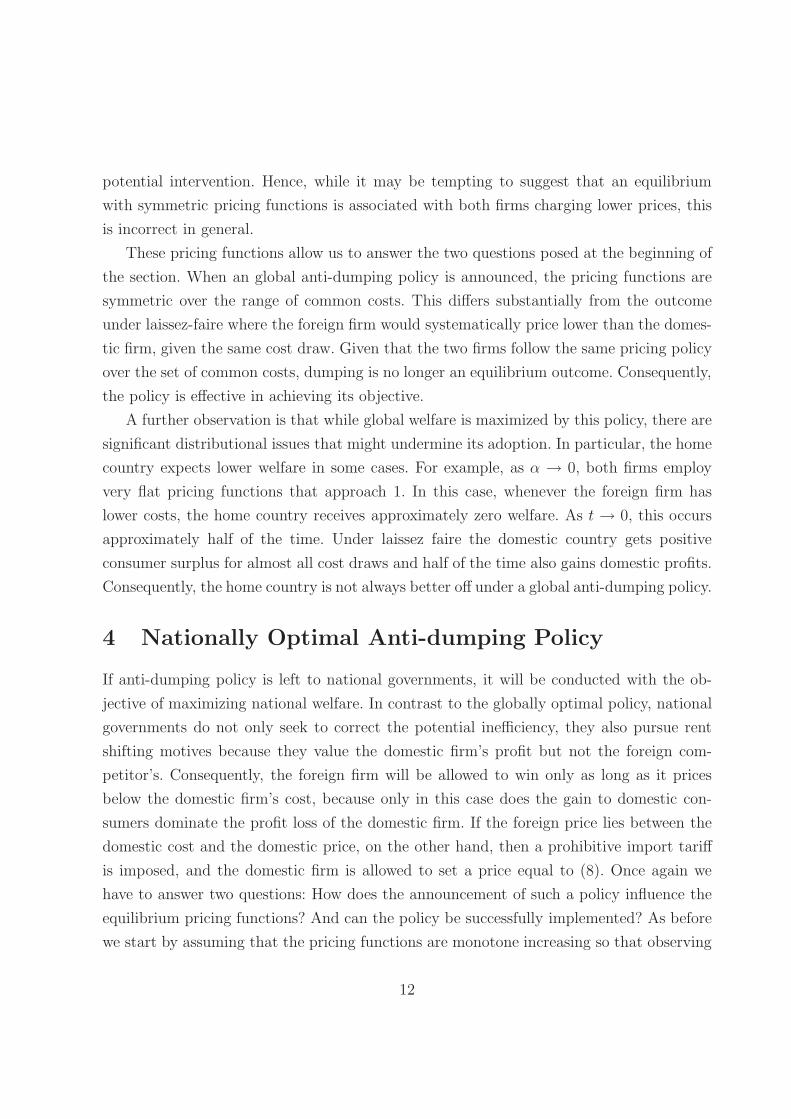
potential intervention. Hence, while it may be tempting to suggest that an equilibrium

with symmetric pricing functions is associated with both firms charging lower prices, this

is incorrect in general.

These pricing functions allow us to answer the two questions posed at the beginning of

the section. When an global anti-dumping policy is announced, the pricing functions are

symmetric over the range of common costs. This differs substantially from the outcome

under laissez-faire where the foreign firm would systematically price lower than the domes-

tic firm, given the same cost draw. Given that the two firms follow the same pricing policy

over the set of common costs, dumping is no longer an equilibrium outcome. Consequently,

the policy is effective in achieving its objective.

A further observation is that while global welfare is maximized by this policy, there are

significant distributional issues that might undermine its adoption. In particular, the home

country expects lower welfare in some cases. For example, as α → 0, both firms employ

very flat pricing functions that approach 1. In this case, whenever the foreign firm has

lower costs, the home country receives approximately zero welfare. As t → 0, this occurs

approximately half of the time. Under laissez faire the domestic country gets positive

consumer surplus for almost all cost draws and half of the time also gains domestic profits.

Consequently, the home country is not always better off under a global anti-dumping policy.

4 Nationally Optimal Anti-dumping Policy

If anti-dumping policy is left to national governments, it will be conducted with the ob-

jective of maximizing national welfare. In contrast to the globally optimal policy, national

governments do not only seek to correct the potential inefficiency, they also pursue rent

shifting motives because they value the domestic firm’s profit but not the foreign com-

petitor’s. Consequently, the foreign firm will be allowed to win only as long as it prices

below the domestic firm’s cost, because only in this case does the gain to domestic con-

sumers dominate the profit loss of the domestic firm. If the foreign price lies between the

domestic cost and the domestic price, on the other hand, then a prohibitive import tariff

is imposed, and the domestic firm is allowed to set a price equal to (8). Once again we

have to answer two questions: How does the announcement of such a policy influence the

equilibrium pricing functions? And can the policy be successfully implemented? As before

we start by assuming that the pricing functions are monotone increasing so that observing

12

the bid allows the government to infer the respective costs.7

Provided that the foreign firm only serves the market if its price is below the domestic

firm’s cost, the foreign firm’s profit takes the form:

π2(p2, c2) = [1 − F1(p2)](p2 − c2 − t) (15)

Note that the foreign firm’s profit is independent of p1, and therefore independent of the

domestic firm’s pricing behavior. We can therefore solve the foreign firm’s profit maximiza-

tion problem separately.

Lemma 3 If a foreign firm for which c2 ∈ [0, 1 − t] enters and a national government

intervenes according to (8) as to maximize domestic welfare, the foreign firm’s pricing and

inverse pricing functions are respectively given by

p2(c2) =1 + c2 + t

2, φ2(p2) + t = 2p2 − 1. (16)

Proof: For an interior solution, the first order condition is given by

∂π2

∂p2= [1 − F1(p2)] − F ′

1(p2)(p2 − φ2(p2) − t) = 0 (17)

which implies the following inverse bid function

φ2(p2) + t = p2 −1 − F1(p2)

f1(p2). (18)

Assumption 1 implies (16).

We now turn attention to the domestic firm’s behavior. Given the foreign firm’s strategy,

the domestic firm’s profit function takes the following form:

π1 =

p1 − c1 if p1 ≤ (1 + t)/2,

[1 − F2(φ2(p1))](p1 − c1)+

[F2(φ2(p1)) − F2(φ2(c1))](p1 − c1) else,

(19)

where p1 (see (8)) is the price that the government allows the domestic company to charge

in case of policy intervention, as before. As long as the domestic firm charges a price below

7Note that we need this assumption only for the domestic pricing function.

13

the lowest foreign price, that is p1 ≤ p2(c2 = 0) = (1 + t)/2, it wins the market for sure,

which leads to profits of p1 − c1. If the domestic price lies above the threshold, there is a

probability that it wins the market outright, represented by the first term in the second

case of equation (19), or it may win due to national policy intervention, which is reflected

by the second term in the second case of equation (19). We now derive the domestic firm’s

optimal pricing strategy resulting from the above profit function.

Proposition 2 If the national government maximizes national welfare and intervenes ac-

cording to (8) with

α ∈(

1

2,

1

1 + t

]

a foreign firm for which c2 ∈ [0, 1 − t] enters and the domestic firm’s pricing function is

given by

p1(c1) = c1 +1 − c1

2α. (20)

Proof: See Appendix A.3.

Why do we have a tighter restriction on α compared to the globally optimal policy?

First, given foreign pricing behavior, the domestic firm can win for sure if it charges

(1 + t)/2. This is unprofitable only if the price p1 imposed by the authority is not too

close to the cost but leaves a substantially large profit. This is the reason for the upper

bound on α. Second, if α were small, the domestic firm would receive a profit close to its

posted price in case of intervention. Since the domestic firm loses only if its price is above

its rival cost, it would go for the maximum (unity) price for a low α, and not only if α = 0

as in the case of globally optimal policies.

What are the consequences of a national anti-dumping policy? There is the possibility

of inefficiency, that is, the higher cost firm ends up serving the market. Note that it can

never be the case that the foreign firm serves the market as the higher cost firm, instead

the national policy creates the possibility that domestic firm will be the high cost firm.

Appendix A.3 shows that the probability of an inefficient outcome is given by (1 − t)2/4.

We are now able to compare the probabilities of inefficient outcomes in the laissez faire

equilibrium (see the dashed line in Figure 2) and for the nationally optimal policies (see

the solid line in Figure 2).

14

0.2 0.4 0.6 0.8 1t

0.05

0.1

0.15

0.2

0.25probability

Figure 2: Comparison of inefficiency probabilities under national and laissez faire regimes

Figure 2 shows that the inefficiency probability is much larger for low levels of t for the

nationally optimal policy. However, it is lower for large levels of t. The reason is that the

nationally optimal policy will also intervene when trade costs are low if the foreign price,

and not foreign overall cost, is larger than the domestic cost. In this case, intervention

for a global perspective is not urgent. For higher trade costs, the foreign firm charges a

higher price, and thus the probability of winning is low. This is in contrast to the laissez

faire regime in which the foreign firm prices more aggressively. Therefore, the nationally

optimal policy has a lower inefficiency probability in this range.

5 Concluding remarks

This paper has developed an efficiency theory of dumping and anti-dumping. We could

show that there is a case for policy intervention if firms compete by prices under incomplete

information. The reason is that the foreign firm is more aggressive without intervention.

In case of a globally optimal policy, dumping will not occur because both firms employ

the same pricing strategy across the common range of overall costs. Thus, the policy does

not have to be applied but its announcement to apply it in the relevant cases is already

successful. In case of a nationally optimal policy, only the domestic firm can be the source

of inefficiency, and inefficiency is likely to occur for low trade costs compared to the laissez

15

faire. This observation strengthens the need for global policy coordination of antidumping

policies if markets become more integrated.

Appendix

A.1 Equilibrium pricing strategies without antidumping mea-

sures

In case of entry, let γ, γ ∈ [0, 1 − t] denotes the critical foreign type which is indifferentbetween entry and no entry. We will determine γ below. Given that the domestic firmknows the size of g and can observe this investment, it will update its beliefs if it observesentry such that the foreign types which enter will be uniformly distributed between 0 andγ. Consequently, the expected profits of both firms are equal to

π1(p1; c1) =

(

1 − φ2(p1)x

γ

)

(p1 − c1), (A.1)

π2(p2; c2) = (1 − φ1(p2))(p2 − c2 − t).

First, let us establish that both firms will employ a price strategy such that the optimalprice functions have a common upper and lower bound for those prices by which each firmis able to win demand. Let the lower (upper) bound be denoted by p(p). If pi = p, firmi will win with certainty, so there is no reason to undercut this price. This confirms thecommon lower price bound, and hence φ1(0) = φ2(0) = p. Suppose that the first-orderconditions (3) are fulfilled for all pi ∈ [p, p]. We will now establish that

p =1 + t + γ

2, (A.2)

φ1(p) =1 + t + γ

2, φ2(p) = γ

φ1(p1) = c1, ∀p1 ∈ [p, 1]

are part of the equilibrium pricing strategies. Note that (A.2) specifies that the domesticfirm charges its cost for all prices above p; in these cases, the domestic firm cannot win themarket and will be beaten by the foreign firm with probability one. As we have assumedthat the first-order conditions hold up to p, we have to prove that no firm is better offby charging a higher price. As for the domestic firm, π1(p; p) = 0 because it will win withzero probability. A higher price leads also to zero profits as it does not change the zero winprobability; hence, the domestic firm has no incentive to deviate from this strategy. Theforeign firm is supposed to charge p for c2 = γ. Given that the domestic firm charges itscost for all prices above p, the foreign firm profit is equal to

π2(p; γ) = (1 − p)(p − γ − t) =(1 − t − γ)2

4(A.3)

16

if it follows the prescribed strategy and

π2(p2 > p; γ) = (1 − p2)(p2 − γ − t)

if it charges a higher price. Maximizing π2(p2 > p; γ) over p2 leads to an optimal p2 = p,and hence also the foreign firm has no incentive to deviate.

For all p1, p2 ∈ [p, p], the first-order conditions for (A.1) are

γ − φ2(p1) − φ′

2(p1)(p1 − c1) = 0,

1 − φ1(p2) − φ′

1(p2)(p2 − c2 − t) = 0.

Note that each first-order condition depends on both inverse price functions. We now followa solution concept similar to Krishna (2002) as to determine the boundary conditions and tosimplify the differential equations. In equilibrium, ci = φi(pi), and using p as the argumentin the inverse price functions allows us to rewrite the first-order condition as

(φ′

1(p) − 1)(p − φ2(p) − t) = 1 − φ1(p) − p + φ2(p) + t,

(φ′

2(p) − 1)(p − φ2(p)) = γ − φ2(p) − p + φ1(p).

Adding up yields

−d

dp(p − φ1(p))(p − φ2(p) − t) = 1 + t + γ − 2p, (A.4)

and integration implies

(p − φ1(p))(p − φ2(p) − t) = p2 − (1 + t + γ)p + K, (A.5)

where K denotes the integration constant. We can determine K by using the upper bound-ary condition. For p = p, the LHS of (A.5) is zero and we find that

K =(1 + t + γ)2

4,

so that (A.5) reads

(p − φ1(p))(p − φ2(p) − t) = p2 − (1 + t + γ)p +(1 + t + γ)2

4(A.6)

in equilibrium. Furthermore, φ1(0) = φ2(0) = p so that

p(p − t) = p2 − (1 + t + γ)p +(1 + t + γ)2

4

17

which leads to

p =(1 + t + γ)2

4(1 + γ). (A.7)

We can use (A.6) as to rewrite the first-order conditions such that each depends on a singleinverse price function only:

γ − φ2(p) = φ′

2(p)p2 − (1 + t + γ)p + (1+t+γ)2

4

p − φ2(p) − t= 0, (A.8)

1 − φ1(p) = φ′

1(p)p2 − (1 + t + γ)p + (1+t+γ)2

4

p − φ1(p)= 0.

Eqs. (A.2), (A.7) and (A.8) completely describe the equilibrium behavior of both firmsin terms of their inverse price functions.8 Hence, they represent the solution to Stage IIof our game, given that no intervention will occur. As for stage I, eq. (A.3) allows us todetermine the critical type γ which will be indifferent between entry and no entry. Thistype’s expected profit must be equal to the investment g such that

γ = 1 − t − 2√

g.

An interior solution requires that 2√

g < 1− t. More importantly, as we deal with marketsto which entry is easy, γ ≃ 1 − t for a g sufficiently close to zero. For γ ≃ 1 − t, (A.8)simplifies to

1 − t − φ2(p) = φ′

2(p)(1 − p)2

p − φ2(p) − t, (A.9)

1 − φ1(p) = φ′

1(p)(1 − p)2

p − φ1(p).

Because prices must not fall short of overall costs, φ′

1, φ′

2 > 0, and hence the solutionsto (A.9) satisfy that the (inverse) price functions increase with the costs (prices). Solvingthese equations gives the inverse price functions

φ1(p) = 1 − 2(1 − p)

1 − 2(1 − p)2K1

(A.10)

φ2(p) = 1 − 2(1 − p)

1 − 2(1 − p)2K2− t, (A.11)

8It is possible to derive explicit solutions for the inverse price functions. These functions, however,cannot be inverted as to solve for the price functions. The results are available upon request.

18

where the Ki’s are the constants of integration. Note that the domestic firm’s price policywill no longer include a range of prices in which it will charge its cost (and win with zeroprobability) because

p = 1 and p =1

2 − t

for γ ≃ 1 − t. Using the last condition, that is φ1(0) = φ2(0) = 1/(2 − t), we find that

K1 =1

2

t(2 − t)

(1 − t)2≥ 0 and K2 = −K1 ≤ 0.

Plugging K1 and K2 back into (A.10) and solving for p yields (5).To determine the probability that an inefficient outcome occurs, conditional upon entry

of the foreign firm, we define the borderline c2(c1) between the inefficient and the efficientset of cost draws at which the resulting prices are equal. Setting p1 and p2 in (5) equal toeach other gives

c2(c1) = 1 − 1 − c1√

1 − (2 − t) t (2 − c1) c1

(1 − t)2

− t. (A.12)

The foreign firm prices more aggressively if c2(c1) + t ≤ c1 which is equivalent to

(1 − c1)

1 − 1 − c1√

1 − (2 − t) t (2 − c1) c1

(1 − t)2

≥ 0

⇔

√

1 − (2 − t) t (2 − c1) c1

(1 − t)2 ≥ 1

⇔ 1 − (2 − t)t(2 − c1)c1 ≥ (1 − t)2. (A.13)

Note that the LHS decreases with c1 and is thus at least equal to 1− 2t + t2 = (1− t)2 orlarger which completes the proof for Lemma 2.

The probability of inefficiency can be best derived from two graphs in the c2−c1−space.Figure 3 shows equation (A.12) for t = 0.2 as the solid line. The broken line is the efficiencyborder c2 = c1 − t where both firms are equally efficient. For c1 < t, the domestic firm isthe efficient one in any case. In the laissez faire equilibrium, the foreign firm wins (loses) ifc2 < (>)c1, and the domestic firm should win from a global perspective if c2 > c1 − t. Thearea between the two lines represents the inefficiency. Note that the size of the rectangle is1− t due to the upper bound for c2. The probability of inefficiency can thus be computedas the area below the solid line minus the area below the broken line, corrected by thefactor 1/(1 − t):

19

0.2 0.4 0.6 0.8 1c1

0.2

0.4

0.6

0.8c2

Figure 3: Inefficiency in the laissez faire equilibrium

1

1 − t

(∫ 1

0

c2(c1)dc1 −∫ 1

t

(c1 − t)dc1

)

=1

2+

1

(2 − t)(1 − t)− 1

1 − t. (A.14)

A.2 Globally optimal anti-dumping policies

Our proof proceeds in two steps. First, we assume that all foreign firm for which c2 ∈[0, 1 − t] will enter. Second, we will show that no foreign firm for which c2 ∈ [1 − t, 1] canbe better off by entering, and no foreign firm for which c2 ∈ [0, 1 − t] can be better off bynot entering. In the main text, we have discussed the first derivative of the domestic firmw.r.t. its price in detail (see equation (12). The corresponding expression for the foreignfirm reads

∂π2

∂p2= [1 − F1(c2 + t)] > 0

if φ1(p2) ≤ c2 + t, (A.15)

∂π2

∂p2= [1 − F1(φ1(p2))] − F ′

1φ′

1(p2 − p2) + (1 − α)(F1(φ1(p2)) − F1(c2 + t))

if φ1(p2) > c1 + t. (A.16)

20

Assume that both the first case of (12) and (A.15) are not binding. Given Assumption 1,we find for our candidate pricing functions (13) that profits can be written as

π1 =2(1 + αc1) − (1 + α)p1

1 − t,

π2 = (p2 − c2 − t)(2 − (1 − α)(c2 + t) − (1 + α)p2) (A.17)

if the constraints imposed by the first case of (12) and (A.15) do not bind. In (A.17),we assume for the domestic (foreign) profit that the domestic (foreign) firm expects theforeign (domestic) firm to charge a price according to (13). Maximization of these profitsw.r.t. p1 and p2 reproduces (13). Furthermore,

φ2(p1) = c1 ⇔ p1 =1 + α(c1 + t)

1 + α<

1 + αc1

1 + α,

φ1(p2) = c2 ⇔ p2 =1 + α(c2 + t)

1 + α=

1 + α(c2 + t)

1 + α,

so that both the first case of (12) and (A.15) are not binding (or just not binding forthe foreign firm). Hence, our candidate pricing functions (13) are mutually consistent asthey set both the second case of (12) and (A.16) equal to zero for the common range ofoverall costs. Furthermore, they are increasing in costs. Note, however, that the domesticfirm will win with certainty if c1 ∈ [0, t]. Hence, the domestic firm will not lower its pricebeyond p1(c1 = t) as it cannot increase its win probability any further. This proves thatthe pricing function are optimal if all foreign firm for which c2 ∈ [0, 1 − t] will enter, andall other firms will stay away. Now note that the any foreign firm for which c2 ∈ [1 − t, 1]cannot make any profit by entering as its break even price is unity. Furthermore, no firmfor c2 ∈ [0, 1− t] cannot be better off by not entering as there is a positive probability thatit will win the market. This completes the proof of Proposition 1.

A.3 Nationally optimal anti-dumping policies

Below the lowest price of the foreign firm, the domestic firm’s profit function is strictlyincreasing in p1. This implies that the domestic firm will never set a price below (1 + t)/2but instead charge (1 + t)/2 which leads to profits of π1 = (1 + t)/2 − c1.

Above the threshold, the first order condition for the second case in (19) leads to (20).Note that this function is monotonically increasing as long as α > 1/2. For α = 1/2 thedomestic firm charges a price of one, independent of its cost draw. For a lower α, that is,when the government allows the domestic firm to charge a relatively high price in caseof intervention, the first order condition would imply a decreasing price above unity, butgiven our assumption that the willingness to pay is bounded at one, it charges a price ofone for all α ≤ 1/2.

21

For α > 1/2 we need to check that the profit resulting from the above pricing ruleexceeds the profit π1 that the firm would obtain by charging the lowest price of the for-eign competitor. Plugging (20) back into the second case of (19) results in the followingcondition:

π∗

1 =(1 − c)2

2(1 − t)α≥ π1 =

1 + t

2− c. (A.18)

This condition is satisfied for all cost draws c1 ∈ [0, 1] as long as α ≤ 1/(1 + t). As in thecase of globally optimal policies, any foreign firm for which c2 ∈ [1− t, 1] cannot make anyprofit by entering as its break even price is unity. Furthermore, no firm for c2 ∈ [0, 1 − t]cannot be better off by not entering as there is a positive probability that it will win themarket. This completes the proof of Proposition 2.

0.2 0.4 0.6 0.8 1c1

0.2

0.4

0.6

0.8c2

Figure 4: Inefficiency for nationally optimal policies

As for the inefficiency probability, we proceed similarly as in Appendix A.1. Figure 4also shows the efficiency border as a broken line for t = 0.2. However, now the domesticfirm is the source of potential inefficiency. Setting (16) and (20) equal to each other, weget a critical c2 = 2c1 − (1 + t) which is given by the solid line. This line gives the costsfor which both firms charge the same prices ,and hence the domestic firm wins if c2 islarger. This function is only defined for c1 ∈ [(1 + t)/2, 1]. The probability of inefficiencyis given by the area below the broken line minus the area below the solid line, correctedby 1/(1 − t):

1

1 − t

(

(1 − t)2

2− 1

2

(

1 − 1 + t

2

)

(1 − t)

)

=(1 − t)2

4. (A.19)

22

References

Anderson, J. E. (1992). Domino dumping, i: competitive exporters. American EconomicReview, 82 (1), 65–83.

Blonigen, B. A. and Prusa, T. J. (2004). Antidumping. In Choi, E. and Harrigan, J. (Eds.),Handbook of International Trade, pp. 251–284. Blackwell.

Bown, C. P. (2007). Global antidumping database. World Bank, Development ResearchGroup, Trade Team, Washington, D.C. :.

Brander, J. and Krugman, P. (1983). A ’reciprocal dumping’ model of international trade.Journal of International Economics, 15 (3-4), 313–321.

Kolev, D. R. and Prusa1, T. J. (2002). Dumping and double crossing: the (in)effectivenessof cost-based trade policy under incomplete information. International EconomicReview, 43 (3), 895–918.

Matschke, X. and Schottner, A. (2008). Antidumping as strategic trade policy under asym-metric information. Working papers 2008-19, University of Connecticut, Departmentof Economics.

Miyagiwa, K. and Ohno, Y. (2007). Dumping as a signal of innovation. Journal of Inter-national Economics, 71 (1), 221–240.

Staiger, R. W. and Wolak, F. A. (1992). The effect of domestic antidumping law in thepresence of foreign monopoly. Journal of International Economics, 32, 265–287.

23