A THEORETICAL MODEL OF THE THERMAL CONDUCTIVITY OF IDEALIZED SOIL by Anil Misra, Ph.D. Assistant Professor Civil Engineering Department Bryan R. Becker, Ph.D., P.E., Member ASHRAE Associate Professor Mechanical and Aerospace Engineering Department Brian A. Fricke, Student Member ASHRAE Research Assistant Mechanical and Aerospace Engineering Department University of Missouri-Kansas City 5605 Troost Avenue Kansas City, MO 64110-2823

1

A Theoretical Model of the Thermal Conductivity of Idealized Soil Anil Misra, Ph.D., Bryan R. Becker, Ph.D., P.E. (Member ASHRAE) and Brian A. Fricke (Student Member ASHRAE) University of Missouri-Kansas City 5605 Troost Avenue, Kansas City, MO 64110-2823 ABSTRACT Accurate prediction of soil thermal conductivity is of prime importance in the numerical simulation of heat transmission through soils. This paper focuses upon empirical and semi-empirical prediction methods for soil thermal conductivity. A family of empirical correlations are presented which relate soil thermal conductivity to saturation for five soil types: gravel, sand, silt, clay, and peat. These correlations are developed from a database of measured data available in the literature. Also, a theoretical model of soil thermal conductivity is developed for granular materials composed of rotund particles in an almost dry state. This theoretical model includes the effects of the micro-structure and the conductivity of the solid phase. It explicitly relates soil thermal conductivity to dry density and agrees well with experimental data. This paper also presents a review and discussion of those factors which affect soil thermal conductivity, previously reported prediction methods, and conductivity measurement techniques. NOMENCLATURE a Shape function used in Gemant's equation A cross-sectional area of a soil sample b Shape function used in Gemant's equation B Function of dry density in Van Rooyen method c Near-field pore parameter in Eq. (28) C Function of mineral type in Van Rooyen method d Far-field pore parameter in Eq. (28) F Factor in De Vries correlation G Shear modulus of a particle ga Shape factor in De Vries' correlation gb Shape factor in De Vries' correlation gc Shape factor in De Vries' correlation h Apex water h0 Water absorbed as a film around the soil particles

2

H Heat flux at a contact neighborhood H(O) Heat flux through the solid angle O Hc Heat flux through solid contact Hm Heat flux through the moisture bridge Hm Heat flux in the neighborhood of the m-th contact in Eq. (18) k Thermal conductivity of soil ka Thermal conductivity of air kd Soil thermal conductivity in the dry state kf Thermal conductivity of fluid phase kij Effective thermal conductivity tensor ks Thermal conductivity of solid phase (soil particles) ksat Soil thermal conductivity in the saturated state kw Thermal conductivity of water Ke Dimensionless function of soil saturation n Number density of particles n Normal vector at m-th contact in Eq. (18) n Normal vector at m-th contact in Eq. (18) ni(O) Direction cosine of solid angle O nj(O) Direction cosine of solid angle O N Total number of contacts in volume V p Coordination number (number of contacts per particle) P Porosity q Electric power input per unit length of probe Q Electric power input r Radius of contact area R Radius of particle s Function of granulometry in Van Rooyen method S Saturation t1 Time t2 Time vs Volume of a single particle V Volume of representative element in Eq. (18) w Moisture content wu Fractional volume of unfrozen water xf Volume fraction of fluid phase xs Volume fraction of solid phase z Shape function used in Gemant's equation a Ratio of mineral to air thermal conductivities ß Heat flux parameter dij Kronecker delta ?T Temperature difference or change ?X Length of a soil sample f Coordinate angle ? Non-dimensional parameter defined in Eq. (29) ?1 Coefficient in empirical soil thermal conductivity correlation ?2 Coefficient in empirical soil thermal conductivity correlation ?3 Coefficient in empirical soil thermal conductivity correlation ?4 Coefficient in empirical soil thermal conductivity correlation ? Shape function used in Gemant's equation ? Coordinate angle

3

v Poisson's ratio of a particle ?d Dry density ?s Solid density so Isotropic confining stress O Solid angle ? Distribution density function of inter-particle contacts

I. INTRODUCTION

A. Motivation

Numerical simulation of heat transmission through soil requires accurate estimates of soil thermal

conductivity. Soil thermal conductivity estimation methods that could be easily incorporated into computer

models of heat transfer will have a wide variety of applications. The resultant prediction methods will be

valuable in the calculation of heat loss through basements, slabs and crawl spaces, and will thereby improve

the accuracy of hourly building energy analysis programs. Claridge (1988) reports that the impact of earth-

contact heat transfer is comparable with that of infiltration. However, the lack of accessible and accurate

foundation thermal analysis has prohibited realistic comparison of above and below grade energy losses,

thus leading to sub-optimal energy conservation decisions.

Soil thermal conductivity estimation methods will also facilitate the efficient design of ground source

heat pump systems by providing more accurate estimates of thermal energy transfer between the earth loop

heat exchanger and the surrounding soil (Hart and Whiddon 1984). This will lead to better selection of

backfill materials, and optimization of backfill moisture content.

In addition, these estimation methods will assist in assessing the effects of berms on the heat loss from

thermal energy storage tanks (Rosen and Hooper 1989). They will also be useful in the simulation of the

operation of seasonal heat storage in various soil formations which are, by far, the least expensive and most

widely available storage media (Doughty et al. 1983).

Furthermore, the resultant prediction methods will help ensure the safe design and location of

underground storage facilities for nuclear and other hazardous waste materials. Likewise, they will be useful

to designers of buried cables for electric power transmission.

Several empirical and semi-empirical prediction methods for soil thermal conductivity have been

4

proposed. However, most of these methods are not suitable because they apply to only certain soil types

under specific temperature and moisture conditions. Although a large quantity of measured data is available

for various soil types and conditions, very little effort has been made to establish a generally applicable,

semi-empirical soil thermal conductivity prediction method.

B. Scope of this Paper

In this paper, the authors focus upon prediction methods for soil thermal conductivity. In Section II

there is a description of the factors which affect soil thermal conductivity, while in Section III a discussion

of existing prediction techniques is presented.

As a basis for the development of more generally applicable prediction methods, a database of

measured soil thermal conductivity data was created from the existing literature. A description of the

measurement techniques as well as the soil samples used to obtain these data is given in Section IV. Section

V describes an empirical model of soil thermal conductivity, while Section VI presents a theoretical model.

II. FACTORS AFFECTING SOIL THERMAL CONDUCTIVITY

Several factors, such as moisture content, dry density, mineral composition, temperature, and texture,

influence soil thermal conductivity (Kersten 1949, Penner et al. 1975, Salomone et al. 1984, Salomone and

Kovacs 1984, Salomone and Marlowe 1989, Brandon and Mitchell 1989, Mitchell 1991). Moisture content

has a most notable effect upon soil thermal conductivity. As moisture is added to a soil, a thin water film

develops around the soil particles, which bridges the gaps in the soil. This "bridging" increases the effective

contact area between the soil particles, which increases the heat flow and results in higher thermal

conductivity. As more moisture is added, the voids between the soil particles become completely filled with

moisture and the soil thermal conductivity no longer increases with increasing moisture content (Salomone et

al. 1984, Salomone and Kovacs 1984, Salomone and Marlowe 1989). The point at which the maximum

thermal conductivity occurs is called the critical moisture content. For most soils, the critical moisture

content coincides with the optimum moisture content, which is also the state of maximum dry density of the

soil. However, for low density clay soils, the critical moisture content coincides with the plastic limit

5

(Salomone et al. 1984).

Soil thermal conductivity also increases with the dry density of the soil. With an increase in the soil's

dry density, more soil particles are packed into a unit volume and, thus, the number of contact points

between the particles increases. This increase in contact points provides a larger heat flow path resulting in

higher soil thermal conductivity (Salomone et al. 1984, Salomone and Kovacs 1984, Salomone and

Marlowe 1989).

The mineral composition of a soil influences its thermal conductivity. For example, sands with a high

quartz content generally have a greater thermal conductivity than sands with high contents of plagioclase

feldspar and pyroxene (Kersten 1949). Also, soils with high organic content generally have lower soil

thermal conductivity (Salomone and Marlowe 1989).

A dramatic change in soil thermal conductivity occurs at the freezing point when the primary mode of

heat transfer changes from convection to conduction (Kersten 1949, Penner et al. 1975, Salomone and

Marlowe 1989). However, in other temperature ranges the variation of soil thermal conductivity with

temperature is minimal (Brandon and Mitchell 1989). For example, Kersten (1949) reports an average

variation of 4% in soil thermal conductivity over the temperature range from 4.4°C to 21°C. At low

moisture content, the thermal conductivity is higher in the unfrozen state than in the frozen state. However,

the converse is true at high moisture content (Penner et al. 1975).

Soil texture is another factor which may influence a soil's thermal conductivity. For a given moisture

content and dry density, the thermal conductivity of coarse textured, angular grained soils is higher than that

of fine textured soils (Kersten 1949, Salomone and Marlowe 1989). Also, uniformly graded soils exhibit

lower thermal conductivity than well graded soils (Salomone and Marlowe 1989).

III. EXISTING PREDICTION METHODS

Many correlations for estimating soil thermal conductivity have been proposed. Van Rooyen and

Winterkorn (1957), Johansen (1975), De Vries (1952), Gemant (1952), and Kersten (1949), among others,

have all developed correlations for soil thermal conductivity. These correlations vary in complexity, and

6

each method is limited to only certain soil types under specific conditions. Farouki (1986) has published a

survey of these various correlations which is summarized below.

Van Rooyen's correlation (Van Rooyen and Winterkorn 1957), based on data collected from different

types of sand and gravel, is given as follows:

In this expression, k is soil thermal conductivity, W/m-K; S is the degree of saturation; and, B, C, and s are

functions of dry density, mineral type, and granulometry, respectively. The Van Rooyen method is limited

to unfrozen sand and gravel with saturation levels between 1.5% to 10%.

Johansen's correlation (Johansen 1975), which is based on thermal conductivity data for dry and

saturated states at the same dry density, has the following form:

In this correlation, k is soil thermal conductivity, W/m-K; ksat and kd are soil thermal conductivity in the

saturated and dry states, respectively; and Ke is a dimensionless function of soil saturation.

Based on data from Kersten (1949), Johansen derived equations for Ke in terms of saturation, S. For

coarse, unfrozen soil:

For fine, unfrozen soil:

For any type of frozen soil, Ke = S.

Johansen believed that in a dry state, soil thermal conductivity was based upon dry density or porosity.

For dry natural soils, he derived an equation for kd in terms of dry density, ?d, specifically:

For crushed rock material, Johansen found that:

s + 10 B= k1 CS- (1)

k + K ) k - k( =k dedsat • (2)

1.0 + S log 0.7 = Ke (3)

1.0 + S log = Ke (4)

20% 0.947 - 2700

64.7 + 0.135 = k

d

dd ±

ρρ

(5)

7

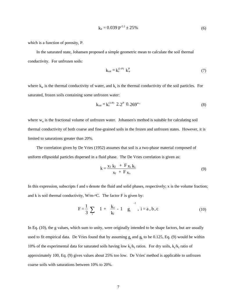
which is a function of porosity, P.

In the saturated state, Johansen proposed a simple geometric mean to calculate the soil thermal

conductivity. For unfrozen soils:

where kw is the thermal conductivity of water, and ks is the thermal conductivity of the soil particles. For

saturated, frozen soils containing some unfrozen water:

where wu is the fractional volume of unfrozen water. Johansen's method is suitable for calculating soil

thermal conductivity of both coarse and fine-grained soils in the frozen and unfrozen states. However, it is

limited to saturations greater than 20%.

The correlation given by De Vries (1952) assumes that soil is a two-phase material composed of

uniform ellipsoidal particles dispersed in a fluid phase. The De Vries correlation is given as:

In this expression, subscripts f and s denote the fluid and solid phases, respectively; x is the volume fraction;

and k is soil thermal conductivity, W/m-°C. The factor F is given by:

In Eq. (10), the g values, which sum to unity, were originally intended to be shape factors, but are usually

used to fit empirical data. De Vries found that by assuming ga and gb to be 0.125, Eq. (9) would be within

10% of the experimental data for saturated soils having low ks/kf ratios. For dry soils, ks/kf ratio of

approximately 100, Eq. (9) gives values about 25% too low. De Vries' method is applicable to unfrozen

coarse soils with saturations between 10% to 20%.

25% P 0.039 = k -2.2d ± (6)

k k = k Pw

P)-(1ssat (7)

2690. 22. k = k wPP)-(1ssat

u (8)

x F+ x

k x F+ k x =k sf

ssff (9)

c , b ,a = i , g 1 - kk + 1

31 = F i

f

s

-1

i

∑ (10)

8

Gemant's correlation (Gemant 1952) is based upon the idealized soil particle shown in Figure 1.

Gemant assumed that the idealized particles made contact only at their apexes and that water collected

around these contact points to form a thermal bridge. Also, heat flow was assumed to be vertically upward.

Gemant's correlation is given as follows:

In Eq. (11), ?d is dry density of soil; w is moisture content; h is the apex water (water collected around the

contact points); h0 is water absorbed as a film around the soil particles; ks is the thermal conductivity of the

solids; kw is the thermal conductivity of water; and a, b, z, and ?(b2/a) are shape functions given by Gemant

(1952). Gemant's method gives reasonable results for unfrozen sandy soils only.

Kersten (1949) tested many soil types and based his correlations on the empirical data he collected.

He produced equations for frozen and unfrozen silt-clay soils and sandy soils. Kersten's correlations for

unfrozen and frozen silt-clay soils are as follows:

The correlations for sandy soils are as follows:

In Eq. (12) and Eq. (13), k is soil thermal conductivity (W/m⋅°C); w is moisture content; and ?d is dry

density (kg/m3). The equations for the silt and clay soils apply for moisture contents of 7% or more; those

for the sandy soils, of 1% or more. Kersten's correlations give reasonable results only for frozen soils with

Ψ ab

a k) z - (1 +

] ) k - k( k[ ) 2 / (h] k / ) k - k( [ tan ]a / )a - (1 [ =

k1 2

s2/1

wsw3/1

2/1wws

-13/4

(11a) h -w 10x 0.16 = h ; 0.078 =a 0d

-32/1d ρρ (11b,c)

2h

a - 1

a = b ;

2h

a

a - 1 = z

3/23/22

3/13/2

(11d,e)

10 ] 0.0288 - w log [0.130 =k :Unfrozen d 0.000624ρ (12a)

w) (10 0.00462 + ) (10 0.0110 =k :Frozen dd 0.000911 0.000812 ρρ

(12b)

10 ] 0.0577 + w log [0.101 =k :Unfrozen d 0.000624 ρ (13a)

w) (10 0.00462 + ) (10 0.0110 =k :Frozen dd 0.000911 0.000812 ρρ

(13b)

9

saturations up to 90%.

As summarized in Table 1, Farouki (1986) has studied the applicability of these methods and has

suggested the conditions under which each method should be used. It is clear that these methods are

applicable only for limited soil types and conditions, and they do not offer a unified, cogent technique for

the estimation of soil thermal conductivity. General purpose numerical models of heat transfer through soil

require unified prediction methods for soil thermal conductivity which are applicable to a wide variety of soil

types. The intent of the study reported in this paper was to develop a prediction method for a variety of soil

types and conditions.

IV. DATABASE OF THERMAL CONDUCTIVITY MEASUREMENTS

A. Measurement Techniques

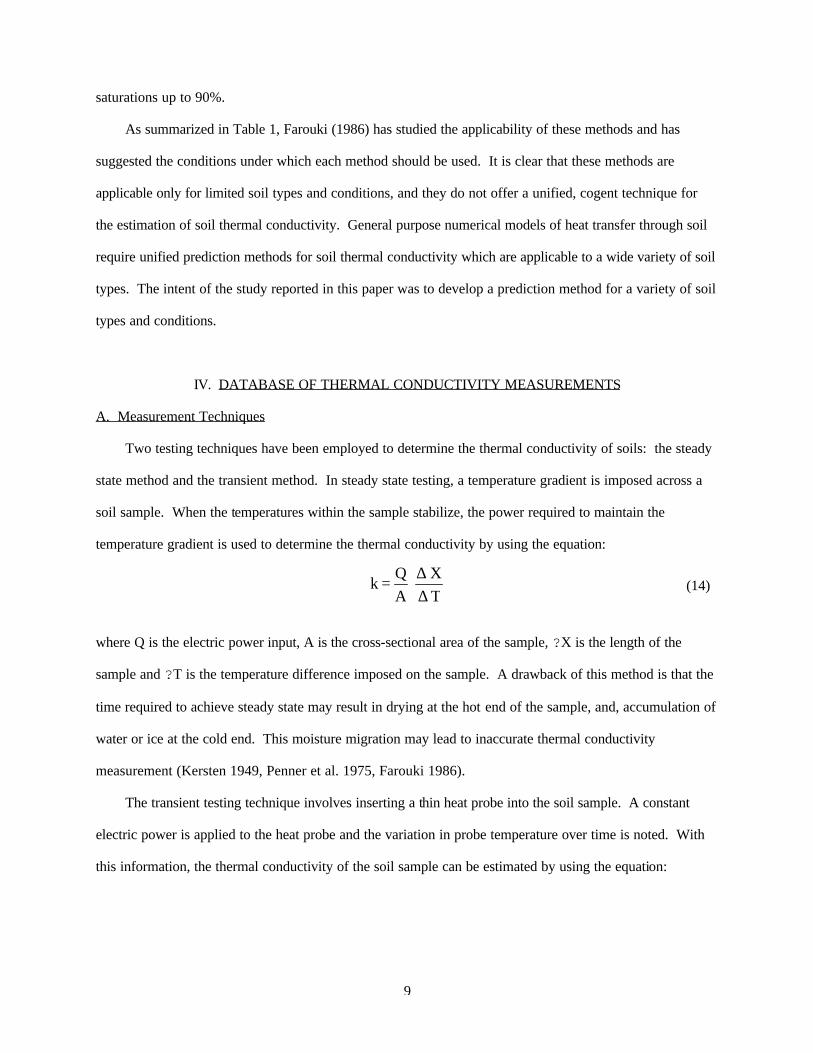
Two testing techniques have been employed to determine the thermal conductivity of soils: the steady

state method and the transient method. In steady state testing, a temperature gradient is imposed across a

soil sample. When the temperatures within the sample stabilize, the power required to maintain the

temperature gradient is used to determine the thermal conductivity by using the equation:

where Q is the electric power input, A is the cross-sectional area of the sample, ?X is the length of the

sample and ?T is the temperature difference imposed on the sample. A drawback of this method is that the

time required to achieve steady state may result in drying at the hot end of the sample, and, accumulation of

water or ice at the cold end. This moisture migration may lead to inaccurate thermal conductivity

measurement (Kersten 1949, Penner et al. 1975, Farouki 1986).

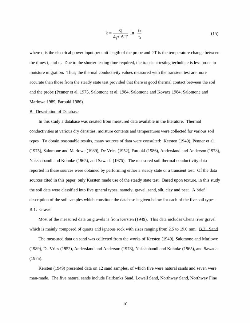
The transient testing technique involves inserting a thin heat probe into the soil sample. A constant

electric power is applied to the heat probe and the variation in probe temperature over time is noted. With

this information, the thermal conductivity of the soil sample can be estimated by using the equation:

T X

AQ

=k ∆∆

(14)

10

where q is the electrical power input per unit length of the probe and ?T is the temperature change between

the times t2 and t1. Due to the shorter testing time required, the transient testing technique is less prone to

moisture migration. Thus, the thermal conductivity values measured with the transient test are more

accurate than those from the steady state test provided that there is good thermal contact between the soil

and the probe (Penner et al. 1975, Salomone et al. 1984, Salomone and Kovacs 1984, Salomone and

Marlowe 1989, Farouki 1986).

B. Description of Database

In this study a database was created from measured data available in the literature. Thermal

conductivities at various dry densities, moisture contents and temperatures were collected for various soil

types. To obtain reasonable results, many sources of data were consulted: Kersten (1949), Penner et al.

(1975), Salomone and Marlowe (1989), De Vries (1952), Farouki (1986), Andersland and Anderson (1978),

Nakshabandi and Kohnke (1965), and Sawada (1975). The measured soil thermal conductivity data

reported in these sources were obtained by performing either a steady state or a transient test. Of the data

sources cited in this paper, only Kersten made use of the steady state test. Based upon texture, in this study

the soil data were classified into five general types, namely, gravel, sand, silt, clay and peat. A brief

description of the soil samples which constitute the database is given below for each of the five soil types.

B.1. Gravel

Most of the measured data on gravels is from Kersten (1949). This data includes Chena river gravel

which is mainly composed of quartz and igneous rock with sizes ranging from 2.5 to 19.0 mm. B.2. Sand

The measured data on sand was collected from the works of Kersten (1949), Salomone and Marlowe

(1989), De Vries (1952), Andersland and Anderson (1978), Nakshabandi and Kohnke (1965), and Sawada

(1975).

Kersten (1949) presented data on 12 sand samples, of which five were natural sands and seven were

man-made. The five natural sands include Fairbanks Sand, Lowell Sand, Northway Sand, Northway Fine

∆

tt ln

T 4q =k

1

2

π (15)

11

Sand, and Dakota Sandy Loam. The Fairbanks sand was a siliceous sand with 27.5% of the particles larger

than 2.0 mm and 70% of the particles between 0.5 and 2.0 mm. The Lowell sand was also siliceous with

particles between 0.5 and 2.0 mm. The two Northway Sands were similar in their composition, with their

main constituent being feldspar, and having grain sizes ranging from 4.75 mm to 0.075 mm. No details are

available on the Dakota Sandy Loam.

Of the seven man-made sands, three were feldspar sands and four were quartz sands. The feldspar

sands consisted of 90% sand-sized particles and 10% gravel-sized particles. The quartz sands included one

sample with grain size larger than 0.5 mm and three samples with grain sizes between 0.5 mm to 2.0 mm.

The sands tested by Salomone and Marlowe (1989) were classified according to the Unified Soil

Classification System (USCS). These sands included well graded sands (SW), poorly graded sands (SP),

silty sands (SM), and clayey sands (SC). However, no information was available concerning their mineral

constituents.

The remaining sands were fine grained sands, however, no information is available on their grain size

distributions or mineral constituents.

B.3. Silt

The measured data on silt is from Kersten (1949) and Salomone and Marlowe (1989). Kersten tested

three silts: Northway Silt Loam, Fairbanks Silt Loam, and Fairbanks Silty Clay Loam. All three silts were

classified as low plasticity silts (ML) according to the USCS. Salomone and Marlowe presented data for

several low plasticity silts. Little information is available about the mineral constituents of these silts.

B.4. Clay

The measured data on clay is from Kersten (1949), Salomone and Marlowe (1989), and Penner et al.

(1975). Kersten tested two clays, Ramsey Sandy Loam and Healy Clay, both of which were classified as

low plasticity clays (CL). The main mineral constituent of these clays is kaolinite. Although Salomone and

Marlowe tested both high and low plasticity clays, no information was given concerning the mineral

composition of these clays. The clay samples tested by Penner et al. were low plasticity clays containing

quartz, illite, chlorite and kaolinite.

12

B.5. Peat

The measured data on peat is from Kersten (1949) and Salomone and Marlowe (1989). Kersten

tested Fairbanks Peat while Salomone and Marlowe tested highly decomposed woody peat.

V. AN EMPIRICAL MODEL OF THERMAL CONDUCTIVITY

Moisture content or saturation has a significant effect upon soil thermal conductivity. Herein we briefly

describe correlations of soil thermal conductivity as a function of saturation which were developed by

Becker et al. (1992).

As depicted in Figure 2, the thermal conductivity of a soil increases in three stages as the saturation

level increases. At low saturations, moisture first coats the soil particles. The gaps between the soil particles

are not filled rapidly and thus there is a slow increase in thermal conductivity. When the particles are fully

coated with moisture, a further increase in the moisture content fills the voids between particles. This

increases the heat flow between particles, resulting in a rapid increase in thermal conductivity. Finally, when

all the voids are filled, further increasing the moisture content no longer increases the heat flow and the

thermal conductivity does not appreciably increase. An empirical model used to describe this behavior is as

follows:

In Eq. (16), S is the saturation; k is the soil thermal conductivity (W/m-°C); and ?1, ?2, ?3 and ?4 are

coefficients which are specified in Table 2 for each of the five soil types in both the frozen and unfrozen

states. At a saturation of zero, Eq. (16) reduces to the following:

Eq. (17) shows that the coefficient ?4 is related to the thermal conductivity of dry soil, kd.

Figures 3 through 7 present the measured soil thermal conductivity versus saturation data for the five

soil types in both the frozen and unfrozen states. The empirical correlations, based upon Eq. (16), are also

plotted on Figures 3 through 7. Three curves have been given for each soil type (except peat). The middle

] ) ( sinh - ) +k ( [sinh = S 4321 λλλλ (16)

λλλ 43d2 = + k (17)

13

curve represents the mean of the measured data. The upper and lower curves approximate the range of

measured data. Due to the small amount of measured data for peaty soils, only a mean correlation is

presented in Figure 7. Measured data collected for gravel includes saturations up to approximately 40% and

thus, the correlations for gravel are valid only to 40% saturation. An error analysis of these correlations is

presented in the work of Becker et al. (1992).

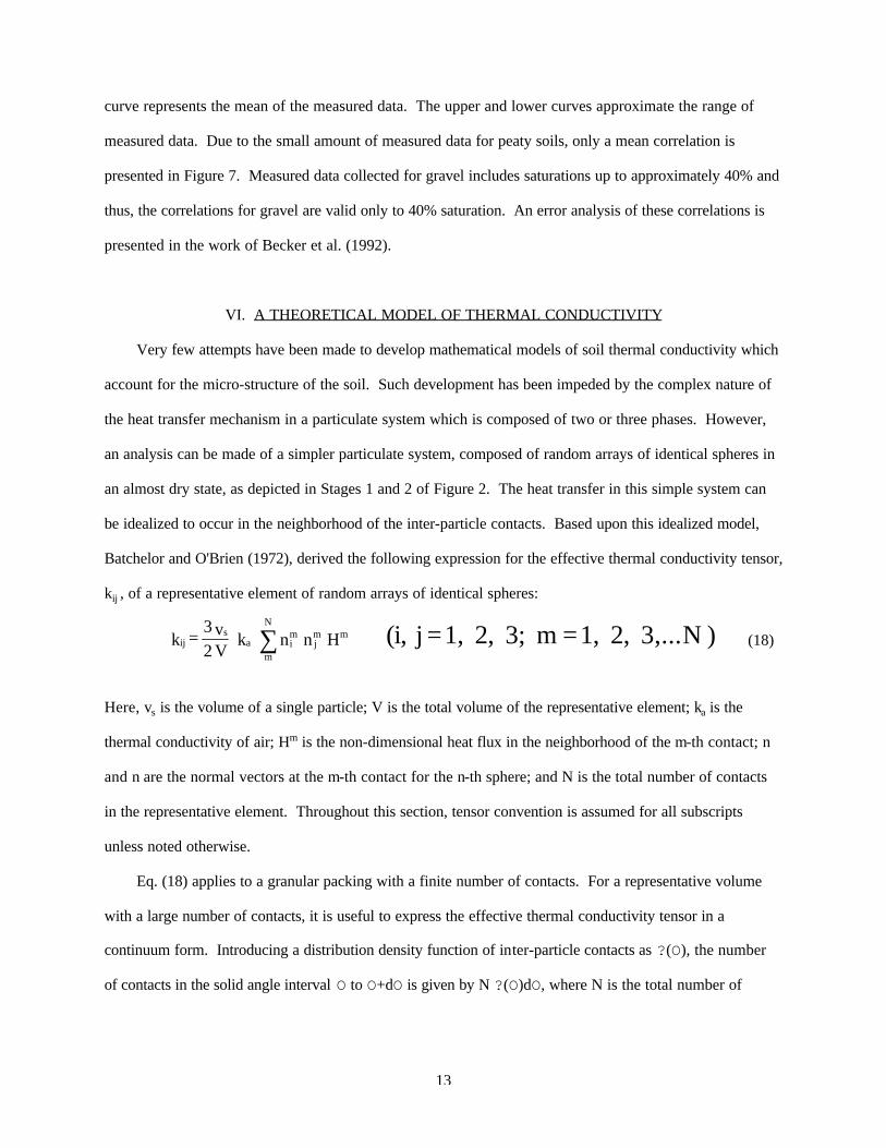
VI. A THEORETICAL MODEL OF THERMAL CONDUCTIVITY

Very few attempts have been made to develop mathematical models of soil thermal conductivity which

account for the micro-structure of the soil. Such development has been impeded by the complex nature of

the heat transfer mechanism in a particulate system which is composed of two or three phases. However,

an analysis can be made of a simpler particulate system, composed of random arrays of identical spheres in

an almost dry state, as depicted in Stages 1 and 2 of Figure 2. The heat transfer in this simple system can

be idealized to occur in the neighborhood of the inter-particle contacts. Based upon this idealized model,

Batchelor and O'Brien (1972), derived the following expression for the effective thermal conductivity tensor,

kij , of a representative element of random arrays of identical spheres:

Here, vs is the volume of a single particle; V is the total volume of the representative element; ka is the

thermal conductivity of air; Hm is the non-dimensional heat flux in the neighborhood of the m-th contact; n

and n are the normal vectors at the m-th contact for the n-th sphere; and N is the total number of contacts

in the representative element. Throughout this section, tensor convention is assumed for all subscripts

unless noted otherwise.

Eq. (18) applies to a granular packing with a finite number of contacts. For a representative volume

with a large number of contacts, it is useful to express the effective thermal conductivity tensor in a

continuum form. Introducing a distribution density function of inter-particle contacts as ?(O), the number

of contacts in the solid angle interval O to O+dO is given by N ?(O)dO, where N is the total number of

)N 3,... 2, 1, = m 3; 2, 1, = j (i, Hnn k V2v3

= k mmj

mi

N

ma

sij ∑ (18)

14

contacts in the representative element of volume V. Thus, the effective thermal conductivity tensor, given in

Eq. (18), can be written in an integral form as follows:

where ni(O) and nj(O) are the direction cosines of the solid angle O, and H(O) is the non-dimensional heat

flux through the solid angle O. In Eq. (19), the integration is performed as follows:

where dO is the solid angle, and ? and f are coordinate angles, as shown in Figure 8. Assuming that the

heat flux, H, at all contact neighborhoods is equal, Eq. (19) can be simplified to:

For isotropic distribution of contacts, the distribution function, ?(O), is given as follows (Misra 1992):

In this case, the effective conductivity tensor becomes:

Noting that dijN/V = pn, Eq. (23) becomes:

where dij is the Kronecker delta (dij=1 for i=j; dij=0 for i≠j), p is the coordination number (number of

contacts per particle) and n is the number of particles per unit volume. In Eq. (24) the terms vs, p and n are

measures of the packing density of a granular assembly. It is useful to replace these terms by more direct

measures of granular media density, namely, the dry density, ?d, and the solid density, ?s. An expression for

the coordination number, p, can be obtained from the void ratio-coordination number relationship reported

ΩΩΩΩΩ∫Ω d )( ) H()(n )(n k V2N v 3

= k jias

ij ξ (19)

θφφππ d d sin ) ( = d ) ( 0 2

0 •∫∫Ω•∫Ω (20)

ΩΩΩΩ∫Ω d)()(n )(n H k V2N v 3

= k jias

ij ξ (21)

π

ξ41

= )(Ω (22)

δ ijas

ij H k V2N v = k (23)

Hk n p v 21

=k as (24)

15

by Chang et al. (1990) and the product vsn can be replaced by ?d/?s to yield the following:

Thus Eq. (24) becomes:

In Eq. (26), the key requirement is the heat flux, H, at a contact neighborhood. Batchelor and O'Brien

(1972) studied the heat transfer through two particles in contact. Based upon their study, an approximate

expression for the non-dimensional heat flux, H, is written as follows:

where Hc is the flux through the solid contact; Hm is the flux through the moisture bridge in the

neighborhood of contact; w is the moisture content; and a is the ratio of mineral to air thermal

conductivities, i.e. km/ka. The non-dimensional heat flux parameter ß may be written as follows:

Here, d depends upon conditions within the pores far from the contact; while c depends upon conditions

near the contact and is more sensitive to the presence of moisture. In Eq. (27), ? is a non-dimensional

parameter, which is defined as follows:

Here, R is the radius of the particle and r is the radius of the contact area. The contact radius depends upon

the loading conditions on the granular medium. For example, under isotropic loading conditions, the contact

radius may be obtained from Hertz-Mindlin contact theory as follows (Chang and Misra 1990):

8 - 21 = p

d

s

ρρ

(25)

Hk 4 - 11 =k a

s

d

ρρ

(26)

βαλλ + ln 2 + )(H w + )(H =H mc (27)

3.9 - c w + d = β (28)

R

r = α

λ (29)

R G p2

)-(1 3 =r o

d

s

3/1

σ

ρνρπ

(30)

16

Here, G is the shear modulus of a particle; v is the Poisson's ratio of the particle; and so is the isotropic

confining stress. Batchelor and O'Brien (1972) have reported simple approximations for fluxes Hc and Hm

depending upon the value of ?, given as follows:

for ? < 1, and

for ? > 1.

By combining Eq. (27) through Eq. (31), it can be seen that as the confining stress, so, approaches

zero, the heat flux contributions, Hc and Hm, become negligible, and the expression for thermal conductivity

may be simplified to:

Eq. (33) shows that thermal conductivity varies linearly with dry density. The measured data exhibits a

similar behavior. Also, Eq. (33) accounts for the presence of moisture at low levels. This behavior is

similar to the experimental results reported by Brandon and Mitchell (1989) for sands with low moisture

content. In Figures 9 and 10, a comparison is presented between the predictions and the measurements for

thermal conductivity versus dry density for quartz and feldspar sands at three levels of moisture content: w

= 0.0%, 0.5%, and 1.0%. In these predictions, the thermal conductivity of a solid particle is taken to be 8.4

W/m-°C and that of air is taken to be 0.026 W/m-°C. The parameter, d, is set to -3.1 for quartz and -3.9

for feldspar, and c is set to 10.5 for quartz and 6.5 for feldspar. As shown in these figures, the model

successfully predicts the same trends as that exhibited by the measured data discussed in Section IV.

VI. CONCLUSIONS

This paper has focused upon prediction methods for soil thermal conductivity. A family of empirical

λλ 2m

2c 0.05- = H ; 0.22 = H (31)

λπλ

ln 2- = H ; 2

= H mc (32)

( )3.9 - wc+ d + ln 2 4 - 11 k =k s

da α

ρρ

(33)

17

correlations has been presented which relates soil thermal conductivity to saturation for five soil types,

namely, gravel, sand, silt, clay, and peat, in both the frozen and unfrozen states. These empirical prediction

methods were developed from a database of soil thermal conductivity measurements available in the

literature. The unified format of these correlations make them readily adaptable to numerical heat transfer

algorithms.

Also, a theoretical model of soil thermal conductivity has been presented which is based upon a micro-

structural approach. Although this model considers a rather simplified particulate system, it gives insight into

the mechanism by which dry density influences soil thermal conductivity. At present, this model is limited

to granular materials in an almost dry state. In spite of this limitation, the model correctly exhibits the

effects of the presence of moisture at low levels.

This paper has also presented a review and discussion of factors which affect soil thermal conductivity,

previously reported prediction methods, and conductivity measurement techniques.

18

REFERENCES Andersland, O.B. and Anderson, D.M. 1978. Geotechnical Engineering for Cold Regions. New York: McGraw Hill. Batchelor, G.W. and O'Brien, R.W. 1972. Thermal or Electrical Conduction Through a Granular Material. Proceedings of Royal Society of London A355:313-333. Becker, B.R., Misra, A. and Fricke, B.A. 1992. Development of Correlations for Soil Thermal Conductivity. International Communications in Heat and Mass Transfer 19:59-68. Brandon, T.L. and Mitchell, J.K. 1989. Factors Influencing Thermal Resistivity of Sands. Journal of Geotechnical Engineering 115 (12):1683-1698. Chang, C.S. and Misra, A. 1990. Application of Uniform Strain Theory to Heterogeneous Granular Solids. Journal of Engineering Mechanics 116 (10):2310-2328. Chang, C.S., Misra, A. and Sundaram, S.S. 1990. Micromechanical Modelling of Cemented Sands Under Low Amplitude Oscillations. Geotechnique XL (2):251-263. Claridge, D.E. 1988. Design Methods for Earth-Contact Heat Transfer. In Advances in Solar Energy, Ed. C.W. Boer, American Solar and Energy Society, Boulder, CO, 305-351. Doughty, C., Nir, A., Tsang, C.F., and Bodvarsson, G.S. 1983. "Heat Storage in Unsaturated Soils: Initial Theoretical Analysis of Storage Design and Operational Method." in Proceedings of the International Conference on Subsurface Heat Storage in Theory and Practice, Stockholm. De Vries, D.A. 1952. The Thermal Conductivity of Soil. Mededelingen van de Landbouwhogeschool te Wageningen 52 (1):1-73, translated by Building Research Station (Library Communication No. 759), England. Farouki, Omar T. 1986. Thermal Properties of Soils. New York: Trans Tech Publications. Gemant, A. 1952. How to Compute Thermal Soil Conductivities. Heating, Piping, and Air Conditioning 24 (1):122-123. Hart, G.K. and Whiddon, W.I. 1984. Ground Source Heat Pump Planning Workshop, Summary of Proceedings, EPRI Report RP 2033-12. Palo Alto: Electric Power Research Institute. Johansen, O. 1975. Thermal Conductivity of Soils. Ph.D. thesis, Trondheim, Norway, (CRREL Draft Translation 637, 1977) ADA 044002. Kersten, M.S. 1949. Thermal Properties of Soils. Bulletin 28, Engineering Experiment Station, Minneapolis: University of Minnesota. Misra, A. 1992. Relationship of Porosity and Elastic Properties for Consolidated Granular Aggregates. in Microstructural Characterization in Constitutive Models for Metals and Soils, ed. G. Voyiadji_, p. 81-94, New York: ASME Press. Mitchell, J.K. 1991. Conduction Phenomena: From Theory to Geotechnical Practice. Geotechnique 41 (3):299-340.

19

Nakshabandi, G. and Kohnke, H. 1965. Thermal Conductivity and Diffusivity of Soils as Related to Moisture Tension and Other Physical Properties. Agricultural Meteorology 2:271-279. Penner, E., Johnston, G.H., Goodrich, L.E. 1975. Thermal Conductivity Laboratory Studies of Some MacKenzie Highway Soils. Canadian Geotechnical Journal 12 (3):271-288. Rosen, M.A. and Hooper, F.C. 1989. A Model for Assessing the Effects of Berms on the Heat Loss from Partially Buried Heat Storage Tanks. Proceedings of the 9th International Heat Transfer Conference, Jerusalem, Israel, August 19-24. Salomone, L.A., Kovacs, W.D., and Kusuda, T. 1984. Thermal Performance of Fine-Grained Soils. Journal of Geotechnical Engineering 110 (3):359-374. Salomone, L.A. and Kovacs, W.D. 1984. Thermal Resistivity of Soils. Journal of Geotechnical Engineering 110 (3):375-389. Salomone, L.A., and Marlowe, J.I. 1989. Soil Rock Classification According to Thermal Conductivity, EPRI CU-6482. Palo Alto: Electric Power Research Institute. Sawada, S. 1975. Temperature Dependence of Thermal Conductivity of Frozen Soil. Kirami Technical College, Kirami, Hokkaido, Japan, Research Report 9(1). Van Rooyen, M. and H.F. Winterkorn 1957. Structural and Textural Influences on Thermal Conductivity of Soils. in Highway Research Board Proceedings 39:576-621.

Table 1. Applicability of Prediction Methodsa

State Texture Saturation Method

Unfrozen Coarse Grained 0.015 - 0.100 0.100 - 0.200 0.200 - 1.000 0.000 - 1.000 saturated

Van Rooyen (except for low-quartz crushed rock) De Vries Johansen Gemant (sandy silt-clay) Johansen, De Vries, Gemant

Fine Grained 0.000 - 0.100 0.100 - 0.200 0.200 - 1.000 saturated

Johansen (underpredicts by 15%) Johansen (underpredicts by 5%) Johansen Johansen, De Vries, Gemant

Frozen Coarse Grained 0.100 - 1.000 saturated

Johansen Johansen, De Vries

Fine Grained 0.000 - 0.900 0.100 - 1.000 saturated

Kersten Johansen Johansen, De Vries

aData from Farouki (1986)

TABLE 2 Correlation Coefficients

Soil Type

Frozen

Unfrozen

?1 ?2 ?3 ?4

Low Mean

High Low Mean

High Low Mean

High Low Mean High

Clay Frozen 23.5 14.5 14.0 1.73 1.73 1.73 -2.0 -2.5 -3.0 -1.75 -2.0 -2.0

Unfrozen 33.5 27.0 14.0 2.01 1.84 2.22 -1.6 -1.5 -3.0 -1.31 -0.97 -1.72

Gravel Frozen 25.4 11.0 11.3 2.01 2.43 2.08 -2.1 -3.0 -2.8 -1.23 -1.6 -0.85

Unfrozen 16.5 6.5 8.3 2.22 2.63 1.39 -1.9 -3.0 -1.8 -1.1 -1.48 -0.8

Peat Frozen 12.0 2.77 -2.6 -2.52

Unfrozen 28.0 6.00 -1.9 -1.4675

Sand Frozen 26.0 10.0 15.0 1.84 1.66 1.18 -1.0 -2.2 -1.8 -0.73

5

-1.625 -0.44

Unfrozen 6.4 6.8 6.8 5.55 2.77 3.47 -3.2 -2.9 -7.5 -2.0 -1.5 -2.0

Silt Frozen 38.0 19.5 18.5 1.66 1.87 1.39 -1.2 -1.8 -2.0 -0.96 -1.53 -1.8

Unfrozen 28.0 17.0 22.0 2.77 2.77 1.73 -1.0 -2.6 -2.2 -0.6 -1.6 -0.95