A STUDY OF ISOTOPIC COMPOSITION OF XYLEM WATER OF WOODY

VEGETATION AND GROUNDWATER ALONG A PRECIPITATION GRADIENT IN

NAMIBIA

A MINI THESIS SUBMITTED IN PARTIAL FULFILMENT OF THE REQUIREMENTS FOR

THE DEGREE

OF

MASTER OF SCIENCE (APPLIED GEOLOGY)

OF

THE UNIVERSITY OF NAMIBIA

BY

Cristofina Mondjila Kanyama

200729586

April 2017

Main Supervisor: Dr. H. Wanke (University of Namibia)

Co-supervisor: Dr. K. Geissler (University of Potsdam, Germany)

ii

Abstract

An understanding of the water used by vegetation in water limited environment is critical to fully

understand water relations of natural areas with vegetation. Such information can be integrated in

water management plans to estimate the influence of groundwater abstraction on the vegetation.

Trees and shrubs are able to access water from: the upper unsaturated soil profile, the capillary

zone of a groundwater store, from nearby streams and rivers. Previous studies have proven that

uptake of water by roots is not associated with isotope fractionation. Stable isotope ratios of

oxygen and hydrogen were analyzed in groundwater, surface water and plant xylem water.

Groundwater samples from the north east part of the country (Enyana and Fair constantia) were

most depleted, while samples from the southern part (Guruchas) were enriched. A very weak

negative correlation (R2=0.07), statistically insignificant (P>0.05) relationship has been noted

between δ18

O values of precipitation and altitude. The estimated depletion rate was 1.3‰ δ18

O

per km. The correlation between distance from the coast and δ18

O composition of precipitation

was negatively weak (R2=0.29) and statistically significant (P<0.05) with an estimated depletion

rate of 0.31 ‰ per 100 km inland. The correlation between longitude and δ18

O composition of

precipitation was very weak (R2=0.016) and statistically insignificant (P>0.05) at roughly 0.09‰

δ18

O depletion per degree. A strong negative correlation (R2=0.64) existed between δ

18O of

precipitation and latitude and it was statistically insignificant (P>0.005). The observed high

variability in δ18

O and δ2H values of groundwater at different sampling sites was attributed

mainly to continental, elevation and amount effect. Both groundwater and xylem water samples

plotted below the GMWL, however plant xylem were more depleted in comparison to

groundwater. Throughout all the sampling sites there was a considerable variation in average

isotope ratio of xylem water of different species examined, but there were still noticeable

iii

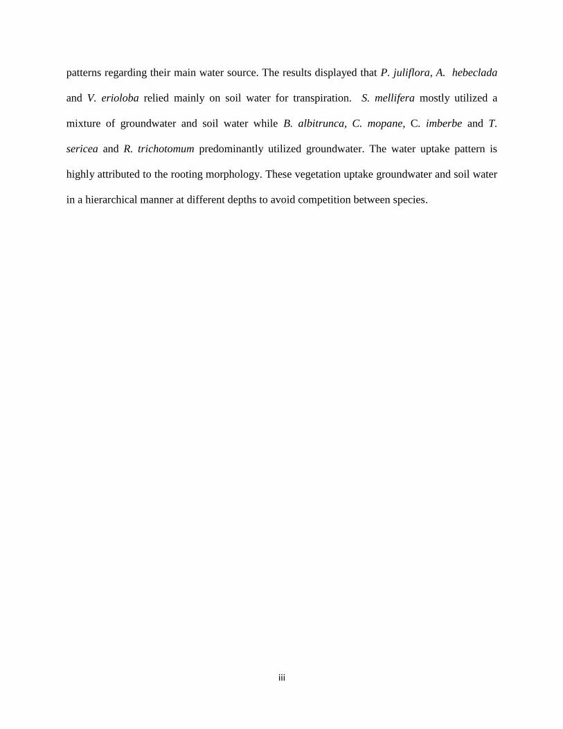
patterns regarding their main water source. The results displayed that P. juliflora, A. hebeclada

and V. erioloba relied mainly on soil water for transpiration. S. mellifera mostly utilized a

mixture of groundwater and soil water while B. albitrunca, C. mopane, C. imberbe and T.

sericea and R. trichotomum predominantly utilized groundwater. The water uptake pattern is

highly attributed to the rooting morphology. These vegetation uptake groundwater and soil water

in a hierarchical manner at different depths to avoid competition between species.

iv

AKNOWLEDGEMENTS

I would like to express my gratitude to my supervisor Dr Heike Wanke and co supervisor Dr

Katja Geissler for the guidance, support and assistance throughout the entire process of writing

the thesis. In addition, I would like to thank Dr Paul Koeniger who performed cryogenic vacuum

extraction and stable isotope analysis on xylem water. I want to thank the entire staff of Geology

department for their guidance through this process. I must also acknowledge Ms. Ungula, Ms.

Hamutoko and all the geology Department students who helped with sample collection. I am also

grateful for the German-Namibian OPTIMASS (Options for sustainable geo-biosphere feedback

management in Savannah systems under regional and global change) which funded this research

project.

v

DECLARATIONS

I, Cristofina M. Kanyama, declare hereby that this study is a true reflection of my own research,

and that this work, or part thereof has not been submitted for a degree in any other institution of

higher education.

No part of this thesis/dissertation may be reproduced, stored in any retrieval system, or

transmitted in any form, or by means (e.g. electronic, mechanical, photocopying, recording or

otherwise) without the prior permission of the author, or The University of Namibia in that

behalf.

I, Cristofina M. Kanyama, grant The University of Namibia the right to reproduce this thesis in

whole or in part, in any manner or format, which The University of Namibia may deem fit, for

any person or institution requiring it for study and research; providing that The University of

Namibia shall waive this right if the whole thesis has been or is being published in a manner

satisfactory to the University.

…………………………………… ……………………………..

Cristofina M. Kanyama Date

vi

Table of Contents

Abstract ........................................................................................................................................... ii

AKNOWLEDGEMENTS.............................................................................................................. iv

DECLARATIONS .......................................................................................................................... v

CHAPTER 1 ................................................................................................................................... 1

1. Introduction ............................................................................................................................. 1

1.1 Overview ........................................................................................................................... 1

1.2 Research problems and objectives ..................................................................................... 7

1.3 Specific objectives of the study ......................................................................................... 7

1.4 Hypothesis ......................................................................................................................... 7

1.5 Significance of the study ................................................................................................... 8

1.6 Limitation of the study ...................................................................................................... 8

CHAPTER 2 ................................................................................................................................... 9

2. Literature review ..................................................................................................................... 9

2.1 The displacement of non-encroacher woody species by encroacher species .................... 9

2.1 Savanna land degradation .................................................................................................. 9

2.2 Groundwater recharge mechanisms ................................................................................. 10

2.3 Previous work done in savanna aquifers ......................................................................... 11

2.4 Methods for estimation of water uptake by plants .......................................................... 12

2.5 Isotopic variation among water sources .......................................................................... 13

CHAPTER 3 ................................................................................................................................. 15

3. Materials and Methods .......................................................................................................... 15

3.1 Study area ........................................................................................................................ 15

3.3 Determination of sampling sites ...................................................................................... 28

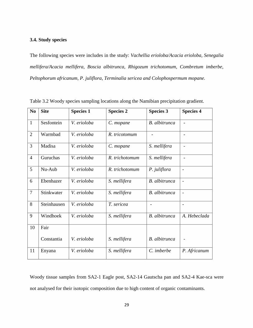
3.4. Study species .................................................................................................................. 29

3.6. Descripion of sampled species ....................................................................................... 31

3.7 Analytical approaches ...................................................................................................... 36

3.8 Statistical analysis............................................................................................................ 40

3.9 Tracing the isotopic composition of precipitation ........................................................... 41

CHAPTER 4 ................................................................................................................................. 42

4. Results ................................................................................................................................... 42

4.1 Isotopic composition of water available for plant uptake ................................................ 42

4.2 Isotopic composition of precipitation .............................................................................. 48

vii

4.3 Precipitation isotopic variation ........................................................................................ 51

4.4 Isotopic composition of woody vegetation xylem water .................................................... 55

4.5 Relationship between plant water source and precipitation amount ............................... 83

4.6 Woody vegetation isotopic composition of all study sites .............................................. 84

4.7 Tree size and depth of water uptake ................................................................................ 86

CHAPTER 5 ................................................................................................................................. 88

5. Interpretation and Discussion ................................................................................................ 88

5.1 Groundwater isotopic variation ....................................................................................... 88

5.2 Isotopic variation in modeled precipitation ..................................................................... 89

5.3 Water uptake by plants .................................................................................................... 93

CHAPTER 6 ................................................................................................................................. 96

6. Conclusions ........................................................................................................................... 96

REFERENCES ............................................................................................................................. 99

viii

List of figures

Figure 1.1 The meteoric relationship of 18

O and 2H in precipitation .............................................. 4

Figure 2.2: Schematic representations of isotope ratios within the soil and groundwater ........... 14

Figure 3.1: Annual average rainfall across Namibia . .................................................................. 16

Figure 3.2: Low pressure system responsible for winter rainfall in the south western part of the

country .......................................................................................................................................... 17

Figure 2.1: The principal vegetation types of Namibia ............................................................... 20

Figure 3.3: Study sites and groundwater basins............................................................................ 22

Figure 3. 4 Simplified geology of Namibia .................................................................................. 27

Figure 3.5: Pale yellow Combretum imberbe tree to the right of a Mopane tree (b) Combretum

imberbe four-winged fruits. .......................................................................................................... 32

Figure 3.6: Peltophorum Africanum . ........................................................................................... 32

Figure 3.7: Acacia hebeclada shrub. ............................................................................................. 33

Figure 3.8: Vachallia erioloba tree................................................................................................ 34

Figure 3.9: Senegallia mellifera shrub. ......................................................................................... 35

Figure 3.10: Boscia Albitrunca tree. ............................................................................................. 35

Figure 3.11: Schematic of a cryogenic extraction line ................................................................. 37

Figure 3.12: Major components of Isotope Ratio Infrared Spectrometer. .................................... 38

Figure 3.13: (a) Schematic of Picarro CRDS analyzer showing how a ring down measurement is

carried out. (b) Demonstrates how optical loss is rendered into a time measurement. ................. 38

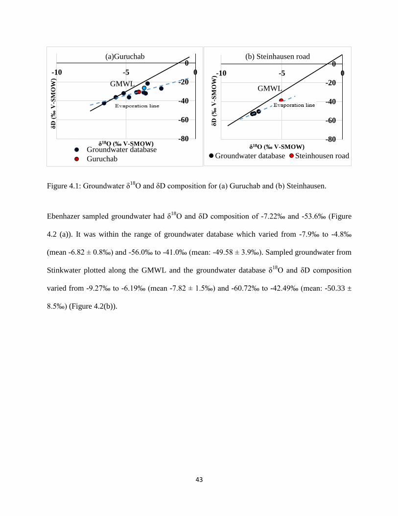
Figure 4.1: Groundwater δ18

O and δD composition for (a) Guruchab and (b) Steinhausen. ....... 43

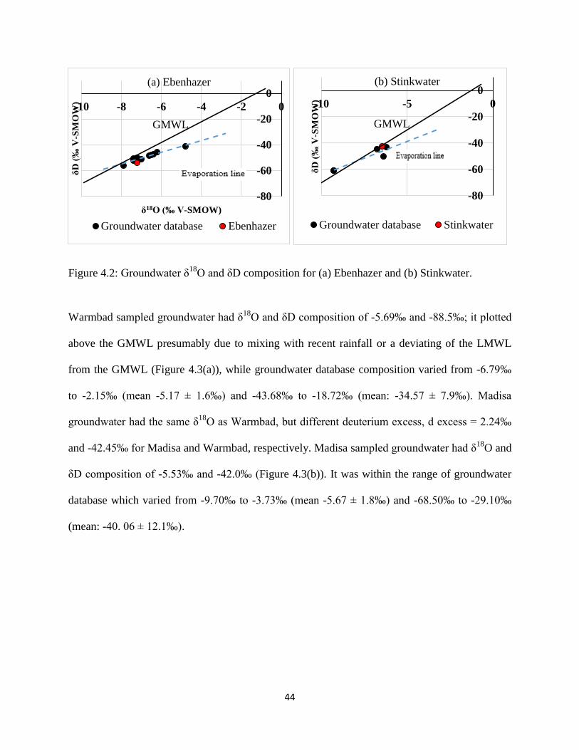
Figure 4.2: Groundwater δ18

O and δD composition for (a) Ebenhazer and (b) Stinkwater. ........ 44

Figure 4.3: Groundwater δ18

O and δD composition for (a) Warmbad and (b) Madisa. ............... 45

Figure 4.4: Groundwater δ18

O and δD composition at (a) Windhoek and (b) Nu-Aub. .............. 45

Figure 4.5: Groundwater δ18

O and δD composition for (a) Enyana, (b) Fair-Constantia and (c)

Seisfontein..................................................................................................................................... 46

Figure 4.6: Groundwater δ18

O and δD composition of all study sites. ......................................... 47

Figure 4.7: Groundwater and calculated source precipitation δD and δ18

O compositions with

reference to GMWL.. .................................................................................................................... 50

Figure 4.8: The relationship between latitude and precipitation δ18

O ......................................... 51

Figure 4.9: The relationship between longitude and precipitation δ18

O ...................................... 52

Figure 4.10 The relationship between distance from the coast and precipitation δ18

O ............... 53

Figure 4.11: The relationship between altitude and precipitation δ18

O ....................................... 53

Figure 4.12 The relationship between annual average rainfall and precipitation δ18

O ................ 54

Figure 4.13: Woody vegetation xylem water and groundwater δD and δ18

O compositions with

reference to GMWL. Linear correlation between groundwater and (b) C. mopane, (b) V.erioloba,

(d) S. mellifera at Madisa. ............................................................................................................. 56

Figure 4.14: Mean δ18

O (‰) for woody vegetation and groundwater at Madisa. ........................ 57

Figure 4.15: Mean δ2H (‰) for woody vegetation and groundwater at Madisa. ......................... 57

Figure 4.16: (a) Woody vegetation xylem water and groundwater δ2H and δ

18O compositions

with reference to GMWL. A biplot of δ18

O – δ2H showing regression relationship between

groundwater (b) B. albitrunca, (c) C.mopane and (d) V. erioloba at Seisfontein. ........................ 59

Figure 4.17: Mean δ18

O (‰) for woody vegetation and groundwater at Seisfontein. .................. 60

ix

Figure 4.18: Mean δ2H (‰) for woody vegetation and groundwater at Seisfontein. ................... 60

Figure 4.19: Figure 4.19 (a) Woody vegetation xylem water and groundwater δ2H and δ18O

compositions with reference to GMWL. A biplot of δ18

O – δ2H showing regression relationship

between groundwater and (b) S.mellifera, (c) B.albitrunca and (d) V. erioloba at Fair Constantia.

....................................................................................................................................................... 62

Figure 4.20: Mean δ18

O (‰) for woody vegetation and groundwater at Fair-Constantia. ........... 62

Figure 4.21: Mean δ2H (‰) for woody vegetation and groundwater at Fair-Constantia. ............ 63

Figure 4.22 Woody vegetation xylem water and groundwater δ2H and δ

18O compositions with

reference to GMWL. ..................................................................................................................... 63

Figure 4.23 Mean δ18

O (‰) for woody vegetation and groundwater at Stinkwater. ................... 64

Figure 4.24: Mean δ2H (‰) for woody vegetation and groundwater at Stinkwater. .................... 64

Figure 4.25: (a) Woody vegetation xylem water and groundwater δ2H and δ

18O compositions

with reference to GMWL. A biplot of δ18

O – δ2H showing regression relationship between

groundwater (b) B. albitrunca, (c) V.erioloba and (d) S. mellifera. ............................................. 66

Figure 4.0-26 Mean δ18

O (‰) for woody vegetation and groundwater at Ebenhazer .................. 66

Figure 4.27 Mean δ2H (‰) for woody vegetation and groundwater at Ebenhazer. ..................... 67

Figure 4.28: Woody vegetation xylem water and groundwater δ2H and δ

18O compositions with

reference to GMWL. A biplot of δ18

O – δ2H showing regression relationship between

groundwater (b) S. mellifera, (c) C. imberbe and (d) P. africanum (e) V.erioloba. ..................... 68

Figure 4.29: Mean δ18

O (‰) for woody vegetation and groundwater at Enyana. ........................ 69

Figure 4.30: Mean δ2H (‰) for woody vegetation and groundwater at Enyana. ......................... 69

Figure 4.31(a) Woody vegetation xylem water and groundwater δ2H and δ

18O compositions with

reference to GMWL. A biplot of δ18

O – δ2H showing regression relationship between

groundwater (b) P. juliflora (c) R. trichotomum and (d) V. erioloba. ......................................... 71

Figure 4.32: Mean δ18

O (‰) for woody vegetation and groundwater at Nu-Aub........................ 72

Figure 4.33: Mean δ2H (‰) for woody vegetation and groundwater at Nu-Aub. ........................ 72

Figure 4.34: (a) Woody vegetation xylem water and groundwater δ2H and δ

18O compositions

with reference to GMWL. A biplot of δ18

O – δ2H showing regression relationship between

groundwater (b) V. erioloba (c) R. trichotomum and (d) S.mellifera and (e) unidentified shrub.

....................................................................................................................................................... 73

Figure 4.35 Mean δ18

O (‰) for woody vegetation and groundwater at Guruchab. ..................... 74

Figure 4.36 Mean δ2H (‰) for woody vegetation and groundwater at Guruchab. ...................... 74

Figure 4.37: (a) Woody vegetation xylem water and groundwater δ2H and δ

18O compositions

with reference to GMWL. A biplot of δ18O – δ2H showing regression relationship between

groundwater and (b) T. cericea (c) V.erioloba at Steinhousen. ................................................... 76

Figure 4.38 Mean δ2H (‰) for woody vegetation and groundwater at Steinhausen. ................... 77

Figure 4.39 Mean δ18

O (‰) for woody vegetation and groundwater at Steinhausen. ................. 77

Figure 4.40: (a) Woody vegetation xylem water and groundwater δ2H and δ

18O compositions

with reference to GMWL at Warmbad. ........................................................................................ 78

Figure 4.41: Mean δ18O (‰) for woody vegetation and groundwater at Warmbad. ................... 79

Figure 4.42: Mean δ2H (‰) for woody vegetation and groundwater at Warmbad. ..................... 79

x

Figure 4.43: (a) Woody vegetation xylem water and groundwater δ2H and δ18O compositions

with reference to GMWL. A biplot of δ18O – δ2H showing regression relationship between

groundwater and (b) B. albitrunca (c) S. mellifera (d) V. erioloba (e) A. hebeclada. ................. 81

Figure 4. 44: Mean δ18O (‰) for woody vegetation and groundwater at Windhoek. ................. 82

Figure 4.45: Mean δ2H (‰) for woody vegetation and groundwater at Windhoek. .................... 82

Figure 4.46 δ18

O and δ2H values of groundwater and plant xylem water of all study sites ......... 85

Figure 4.47: Boxplot of δ18

O values of groundwater and all sampled woody vegetation

throughout the entire country. ....................................................................................................... 85

Figure 4.48: Boxplot of δD values of groundwater and all sampled woody throughout the entire

country.. ........................................................................................................................................ 86

Figure 4.49: Relationship between δ18

O of xylem water and DBH of tree/shrub. ....................... 87

Figure 4.50: The relationship between δ18

O of xylem water and tree/shrub height. .................... 87

List of tables Table 3.1: Groundwater sampling locations along the Namibian precipitation gradient ............. 28

Table 3.2 Woody species sampling locations along the Namibian precipitation gradient. .......... 29

Table 4.1: δ18

O and δD composition of groundwater, deuterium excess and isotopic composition

of recalculated precipitation. ......................................................................................................... 48

Table 4.1 continues. ...................................................................................................................... 49

Table 4.2 The relationship between plant water source (SW: soil water, G: groundwater) and

average annual precipitation along the precipitation gradient. ..................................................... 83

Equations

Equation 1.1: δ2H = 8 δ

18O + 10 ..................................................................................................... 3

Equation 3.1: δ18

O ‰ or δ2H ‰ = (Rsample/Rstandard – 1)*1000 .................................................... 39

Equation 3.2: b = δ2H - (4.5 * δ

18O) ............................................................................................. 41

Equation 3.3: δ2H intercept = δ

2H – m δ

18O ................................................................................. 41

Equation 3.4: δ18

O intercept = (δ2H intercept -b)/a ...................................................................... 41

Equation 5.1: f = (δ18

Ot - δ18

Ogw)/( δ18

Osw- δ18

Ogw) ...................................................................... 75

Appendix

Table A.1: Data used in this study: site, species, xylem water isotopic composition, diameter at

breast& height (1.4 m) and crown diameter. .............................................................................. 107

Table A.2: Groundwater isotopic composition...........................................................................109

1

CHAPTER 1

1. Introduction

1.1 Overview

Namibia Savanna ecosystem covers approximately 64% of the country. In this ecosystem

encroaching and non-encroaching woody species coexist due to vertical partitioning of source

water (Rossato et al., 2014). The study focuses on determining the sources of water uptake of

woody savanna vegetation along Namibia’s precipitation gradient in order to evaluate the water

use strategy of these plants along a precipitation gradient. This helps in achieving an

understanding on hydrogeological processes such as groundwater recharge and water use by

woody vegetation. Natural woody vegetations in arid and semi-arid regions are under stress

owing to lack of water and/or excess salt, therefore to balance water resources for these

vegetation and agriculture it is important to have knowledge on water source transpired by

natural vegetation (Brunel et al, 1995).

Trees and shrubs are able to access water from the upper unsaturated soil profile, the capillary

zone of a groundwater store, or when growing sufficiently close, from nearby streams and rivers

(Eamus, 2006). Stable isotope methods have recently emerged as one of the more powerful tools

for advancing understanding of relationships between plants and their environment (Dawson et

al., 2002). It has been used as a tool for understanding processes in plants such as water use,

water source, and response to different types of water sources, water utilization processes, water

use efficiency and the ability to adopt in arid environments (Yang et al., 2010).

2

The plant water source can be determined by analyzing and comparing stable isotope ratios of

18O/

16O and

2H/

1H in water from plant xylem to potential water sources in the respective focal

study areas. This method emanated from findings by Zimmermann et al. (1967) that uptake of

water by roots is not associated with isotope fractionation, therefore the stable isotopic

composition of plant xylem water represents a mixture of water from different water sources

acquired by all functional roots. This assumption may only be correct for δ18

O as recent research

has shown that in arid environments such as at my study site there may be some fractionation of

the hydrogen isotope while the oxygen isotope ratios of soil water remain unchanged

(Schachtschneider and February, 2013).

1.1.1 Stable isotopes in the hydrological cycle

The 16

O, 17

O, 18

O, 1H and

2H are the stable isotopes that make up the water molecule. These

isotopes of oxygen and hydrogen do not undergo radioactive decay and are therefore stable over

time, hence the name. The most abundant isotope of oxygen on Earth is 16

O, it accounts for

99.76 % of all oxygen, 18

O accounts for 0.2 % of all oxygen and 17

O accounts for the rest.

Meanwhile proteum (1H) accounts for about 99.985 % of all hydrogen and deuterium (

2H)

accounts for 0.015 %.

Water sources can be composed of a range of combinations of 16

O, 18

O, 1H and

2H such as:

1H

1H

16O,

1H

1H

18O,

1H

2H

16O,

1H

2H

18O,

2H

2H

16O,

2H

2H

18O. The molecular weights of each of

these molecules are slightly different, because of the number of neutrons in each nucleus of

3

every atom (Eamus, 2006). The difference in the mass of oxygen and hydrogen isotopes in water

results in distinct partitioning of the isotopes (fractionation) as a result of evaporation,

condensation, freezing, melting or chemical and biological reactions (Kresic, 2008). As a

consequence, different bodies of water have variable ratios of 2H/

1H or

18O/

16O.

When water evaporates from the ocean, lakes and wet surfaces lighter molecules of water

evaporates slightly faster than heavier molecules of water, therefore clouds are slightly depleted

in the heavier isotopes than the water body from which the water evaporated from. When water

condenses and falls as rain, the rain is again slightly enriched in heavier isotopes.

The correlation between 18

O/16

O and 2H/

1H isotope ratios in precipitation on a global scale is

described by the Global Meteoric Water Line (GMWL) (figure 1) developed by Craig (1961) and

expressed by

Equation 1.1: δ2H = 8 δ

18O + 10 (figure 1).

Craig’s line is actually an average of many lines which differ from the global line due to the

varying climatic and geographic parameters. Local lines will differ from the global line in both

slope and deuterium intercept. The Global Meteoric Water Line (GMWL) provides a reference

for interpreting the provenance of groundwaters (Clark and Fritz, 1997).

4

Figure 1.1 The meteoric relationship of 18

O and 2H in precipitation (after Clark and Fritz, 1997).

Stable isotope composition of local precipitation can be described by a Local Meteoric Water

Line (LMWL) (Ingraham, 1998; Jonsson et al., 2009). The ratios 18

O/16

O and 2H/

1H there in are

mainly a function of the place of precipitation. Therefore, Local Meteoric Water line (LMWL)

serves a useful purpose in defining the isotopic composition of the input into hydrological

systems that are fed by meteoric water.

1.1.2 Oxygen and Hydrogen isotopes in soil

The original isotopic composition of infiltrated water and degree of evaporation are the major

factors that influence the soil water. Dawson and Ehleringer (1991) elaborated that variations in

isotopic composition of water within soils can arise because of differences in the seasonal input

of moisture into the soil, evaporation in the uppermost surface or differences between bulk soil

moisture and groundwater.

5

The difference in molecular weight and the fact that different water sources have different

compositions allows comparing the stable isotope composition of water in the plant xylem with

that of water in soil, groundwater and streams and rivers (Eamus, 2006). When xylem water

isotope composition is compared to that of potential sources, it is possible to determine from

which source(s) the water in the xylem was derived. Eamus (2006) further emphasized that this

method is only reliable where differences in isotopic composition are significant. Therefore in

arid and semi-arid climate such as Namibia where fractionation due to evaporation is high, the

method is applicable.

1.1.3 Oxygen and Hydrogen isotopes in vegetation

Plant water source can be estimated by comparing the obtained stable water isotopic ratios to the

GMWL and LMWL. Proportional contribution of the different water sources can then be

estimated using two- or three-layer mixing models; a method proven to be highly accurate by

Yin et al. (2015) during dry periods when the soil water is enriched and isotopically distinct from

groundwater due to isotopic fractionation.

The methodology for using stable isotopes of water to determine water sources of vegetation

relies upon a number of specific assumptions (after Brunel et al., 1995).

There are no significant errors associated with the sampling of isotopes or in the

extraction and analysis of water from plants and soils.

There is no significant variability of isotopic composition in the xylem water within the

tree except in the vicinity of the leaf.

6

The isotopic composition of the soil water is laterally homogeneous within the rooting

area of the tree.

1.1.4 The importance of knowing plant water source

Walker et al. (2001) identified several reasons why it is necessary to know from where plants

source their water:

1. There is a need to fully understand water relations of natural areas with phreatophytic

(deep rooted plants that obtain water from the water table or the layer of soil just above

it) or wetland vegetation.

2. Water use by vegetation may conflict with demands for extraction of groundwater for

industry, or decrease base flow to streams at times of important environmental

requirement.

3. Manipulation of streams for salinity mitigation may affect plant’s reliance on stream

water.

4. Where plantations are being suggested as a means to lower water tables in areas of

salinity.

Over all there is a need to better understand how vegetation responds to change in environment

or how vegetation may modify the environment.

7

1.2 Research problems and objectives

It is not sufficiently known if woody vegetations in savanna ecosystems of Namibia are

accessing water only from the groundwater (groundwater dependent) or from the soil water

reservoir or both. There is currently no correlation existing between plant water source and

precipitation amounts throughout the entire country. Therefore this study is aimed at filling these

knowledge gaps.

1.3 Specific objectives of the study

The objective of the study is to determine the isotopic composition of xylem water of woody

vegetation and groundwater in savanna ecosystems along Namibia’s precipitation gradient. To

assess if woody vegetation in savanna ecosystems in Namibia uptake groundwater or soil water

and how this is controlled by local climate. As well as to assess if typical encroacher species like

Senegalia/Acacia mellifera take water from the same source as non-encroachers such as

Vachalia/Acacia erioloba or Boscia albitrunca.

1.4 Hypothesis

Hypothesis 1: As an adaptation for survival in variable rainfall environments, woody vegetation

of the savanna ecosystem utilizes groundwater in dry areas and soil water in wetter areas.

Hypothesis 2: Encroacher species utilizes soil water and this gives an advantage over non-

encroachers.

8

1.5 Significance of the study

The study will facilitate in assessing the groundwater dependence of the savanna ecosystem. It

will provide a comprehensive understanding on ecological-hydrological interaction between

water sources and woody vegetation. Furthermore it is hoped that that results from this study will

help to understand plant water use mechanisms in arid to semi-arid environments. This

knowledge can help to estimate the influence of groundwater abstraction on the vegetation and

such can be integrated in water management plans.

1.6 Limitation of the study

The plant water sources are identified based on a simple liner mixing models that restricts the

number of water sources to two (groundwater and precipitation) by the assuming isotopically

distinct water sources.

9

CHAPTER 2

2. Literature review

2.1 The displacement of non-encroacher woody species by encroacher species

2.1 Savanna land degradation

Bush encroachment is a form of land degradation that can be found worldwide, but it has been

found to be more prominent in arid and semiarid rangelands (Oldeland et al., 2010). According

to Mannheimer and Curtis (2009) bush encroachment is the invasion of woody species in areas

that have always had either very low densities of trees and shrubs or have been devoid of them. It

is a serious problem throughout much of Namibia, especially in the commercial farming areas of

the north central areas. Bush encroachment negatively affects the efficiency of water use and

groundwater thereby contributing to the process of desertification (Mannheimer and Curtis,

2009).

The cause of bush encroachment is supported by Walter’s two layer- hypothesis (De Klerk,

2004). The theory underlying this model states that the roots of trees are at the surface as well as

the deeper layers of soil, while roots of grasses only occur in the top layer. The hypothesis

suggests preferential rather than exclusive access of roots of trees to water in the subsoil and the

two layers are indirect competition with each other. However if the grass layer is over utilized

mainly by overgrazing, it loses its competitive advantage and can no longer utilize water and

nutrients effectively. This in turn results a higher infiltration rate of water and nutrients into the

subsoil. Such a scenario will benefit trees and bushes only and allow them to be dominant.

10

However Ward (2005) indicated that bush encroachment occurs when disturbances such as:

human impact, fire, herbivory, drought, spatial heterogeneities in water, nutrients and seed

distribution shifts savanna from the open grassland towards the forest end of the environmental

spectrum. Mannheimer and Curtis (2009) argued that rainfall and its variability plays a more

tremendous role in determining vegetation composition than does grazing and that savanna could

be changed to grass dominated land by favorable management and environment conditions.

2.2 Groundwater recharge mechanisms

About 30% of the land area on Earth is arid or semi-arid where potential evapotranspiration

exceeds rainfall (Herczeng and Leaney, 2011). In most arid areas recharge from precipitation is

limited, widely variable and other form of precipitation may not be present at all. The rate of

recharge is the single most important factor in the analysis and management of groundwater

resources in these regions (Kinzelbach et al., 2002). In areas of natural savanna ecosystems

recharge range from 1 to 5 mm year per annum. Herczeng and Leaney, (2011) indicated that

spatial variation in recharge rate occurs with climate, topography, soil, geology, and vegetation.

Groundwater flow pattern is controlled by the configuration of the water table and by the

distribution of hydraulic conductivity in the rocks. The water table in turn is affected by

topography, and is controlled by the prevailing climate (Sophocleous, 2004). In addition, biotic

influences affect most aspects of the hydrologic cycle including groundwater. Vegetation, for

instance regulates the rate at which land surface returns water wapour to the atmosphere.

11

2.3 Previous work done in savanna aquifers

Eco-hydrology is concerned with the importance of hydrological processes in ecosystems and the

effects of plants on hydrological processes (Roberts, 2000). With multiple source of water that

available to plants, it might be expected that the most obvious source is the one preferred for use.

Plants may uptake either soil water or groundwater or both depending on their rooting depths.

Rooting depth and distribution defines the depth to or volume from which plants can potential

extract these water sources (Zencich et al, 2002), however root presence may not be a reliable

indicator of actual water uptake (Dawson and Ehleringer, 1991). Although the opposite could

also be true for instance, Lubis et al. (2004) determined plant water sources using stable water

isotopes method in Riau, Indonesia. The study points out that oil palm absorbed water from the

depth of 0 - 50 cm, which corresponds to the most active root of oil palm that absorbs nutrients,

water and oxygen

Obakeng (2007) pointed out that some vegetations in savanna ecosystem are able to shift from

one water source to another depending on developmental stage and seasonal factor. This was

based on studies by Midgeley et al. (1994) that South African plantain trees, that normally

depends on soil water shifts to groundwater during the drought. Meanwhile in Arizona, Snyder

and Williams (2000) showed that some trees such as Salix gooddiingii used groundwater during

the rainy season in contrast to South African plantain trees.

Vegetations in arid and semi arid communities are often exposed to strong bimodal / summer and

winter rainfall patterns with different isotopic composition. This provide an ideal opportunity to

study the water uptake patterns for by the diverse plant growth forms tat characterise these

12

communities. Studies by Dawson and Ehleringer (1991) have demonstrated that there is a strong

relationship between water source and water use pattern, regardless of the environment.

2.4 Methods for estimation of water uptake by plants

There are several methods for estimating water uptake by plants in arid and semiarid

environments like Namibia. These methods are: direct measurement with lysimeters, water

balance methods, Darcyan methods and environmental tracers such as stable oxygen and

deuterium isotopic method. In this study the latter method will be used.

2.4.1 Direct Measurements with Lysimeters

Lysimeters have been used for determining plant water use by reconstructing the ‘water budget’

by continuously measuring rainfall flux and outflow. The missing term evaporation calculated

deducing recharge from these calculations. The method may be irrelevant in arid regions where

singular recharge features are dominant over areal recharge (Kinzelbach et al., 2002). Eamus et

al. (2002) stressed that lysimeters are difficult to use in natural field conditions, or in an attempt

to replicate natural groundwater conditions.

2.4.2 Water Balance Methods

The water budget is an integral component of any conceptual model of the system under study

Nimmo, (2005). It uses empirical formulas to compute all fluxes involved in the soil water

balance. However this method is highly inaccurate because, recharge is estimated based on the

13

difference between two inaccurately known large quantities: precipitation and

evapotranspiration.

2.4.3 Darcyan methods

Estimate the flux from a head gradient and a hydraulic conductivity. This approach mimics the

infiltration process and can be adapted to any soil, weather conditions or vegetation type

(Kinzelbach et al., 2002).

2.5 Isotopic variation among water sources

There are marked differences in stable isotopic composition due to various water cycles resulting

in distinct difference of δ18

O and δD in various water bodies. These variations can be as large a

200‰ in a in a single location which makes it possible to understand utilization processes, of

various potential water sources, mechanism and co-existence and competition between plats and

neighboring plants (Yang et al., 2010).

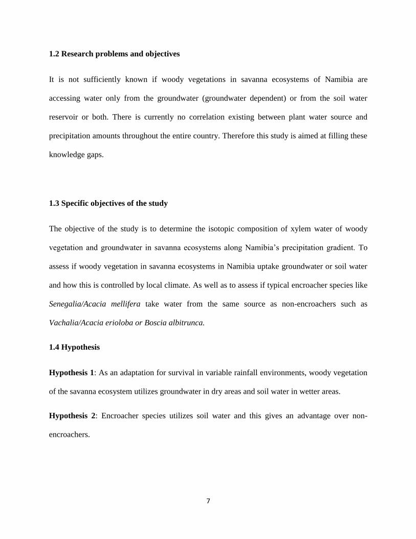
Eamus (2006) showed a typical representation of isotope ratios within the soil and groundwater

(Figure 2.2). They illustrated that near the surface, water is usually enriched in the heavy

isotopes due to evaporation processes and more depleted with increase in depth. For instance,

measuring an isotope value of C within the plant xylem would indicate that all (or most) of the

water used for recent transpiration was sourced from very near the soil surface. If value of A was

to be measured then it would indicate that water must be derived from the water table or

immediately above it. However, if a ratio of value of B was measured in plant xylem, the

14

outcome will show that water was either sourced from the middle of the unsaturated zone (depth

x’) or could be a mixture of water from shallower and deeper depths.

Figure 2.1: Schematic representations of isotope ratios within the soil and groundwater and their

use in discovering plant water source. Black triangle indicates the water table (Eamus 2006).

15

CHAPTER 3

3. Materials and Methods

This is a quantitative study based on stable isotope fractionation, conducted to determine the

plant source water by comparing the isotopic composition of woody Savanna vegetation to that

of potential sources such as groundwater and soil water. Sampling was conducted during the

beginning of the dry season. The dry season is chosen because this is when isotopic variation in

water sources is distinct due to fractionation by evaporation.

3.1 Study area

3.1.1 Climate

Namibia is a driest country in sub-Sahara Africa. Some 22% of Namibia is classified as desert,

while 33% is classified as arid, 37% semi-arid and 8% as semi humid (De Klerk, 2004). Long-

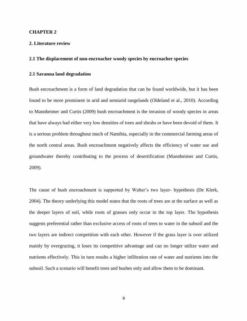
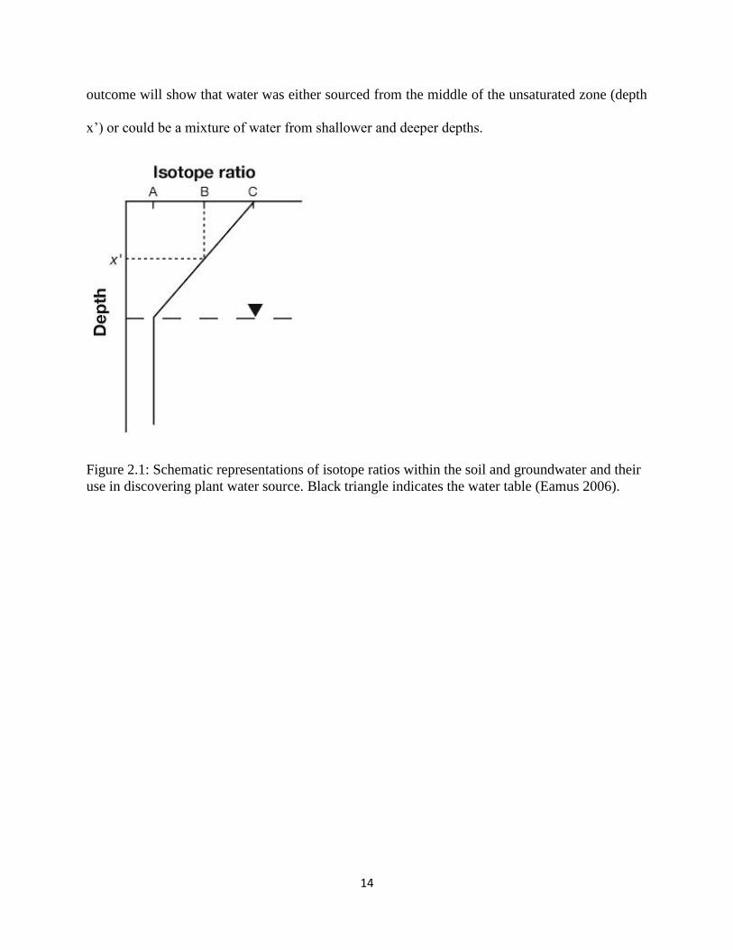
term average rainfall is lowest along the west coast and it gradually increases towards the north-

easterly direction. The annual rainfall varies between 20 mm along the west coast to more than

850 mm in the extreme northeast (Figure 3.7). It rains in summer (October - March) throughout

most of the country except in the extreme south-west where rain more commonly falls in the

winter months (May - August).

16

Figure 3.1: Annual average rainfall across Namibia (adapted from Mendelsohn et al., 2002).

Namibia’s climate is a resultant of various factors including its relative position on the south-

western part of Africa continent spanning a zone between 17o and 29

o south of the equator.

Consequently, Namibia is exposed to air movement driven by three major climatic systems

namely : the Inter-tropical Convergence Zone (ITCZ), the Sub-tropical High Pressure System

and the the Temperature Systen. The Inter-tropical Convergence Zone (ITCZ ) feeds in moisture

17

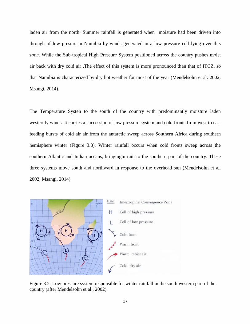
laden air from the north. Summer rainfall is generated when moisture had been driven into

through of low presure in Namibia by winds generated in a low pressure cell lying over this

zone. While the Sub-tropical High Pressure System positioned across the country pushes moist

air back with dry cold air .The effect of this system is more pronounced than that of ITCZ, so

that Namibia is characterized by dry hot weather for most of the year (Mendelsohn et al. 2002;

Msangi, 2014).

The Temperature Systen to the south of the country with predominantly moisture laden

westernly winds. It carries a succession of low pressure system and cold fronts from west to east

feeding bursts of cold air air from the antarctic sweep across Southern Africa during southern

hemisphere winter (Figure 3.8). Winter rainfall occurs when cold fronts sweep across the

southern Atlantic and Indian oceans, bringingin rain to the southern part of the country. These

three systems move south and northward in response to the overhead sun (Mendelsohn et al.

2002; Msangi, 2014).

Figure 3.2: Low pressure system responsible for winter rainfall in the south western part of the

country (after Mendelsohn et al., 2002).

18

3.1.2 Namibia’s Savanna types

According to Giess (1971) Namibia has 14 major vegetation types of which 7 are savanna type.

The savanna range type covers 64 % of the country and can be divided into three main veld

(range) types, namely the dwarf shrub savanna in the central-south, the various acacia-based tree

and shrub savanna associations in the center and eastern parts, and the mopane savanna in the

north-west (Figure 2). The dwarf shrub savanna is characterized by Rhigozum trichotomum,

Catophractes alexandrii, Eriocephalus species and various small Karoo bushes. This area forms

part of the Etosha National Park and supports a diverse and abundant wildlife population.

The mixed tree and shrub savanna of the southern Kalahari is characterized by deep sand

and Acacia haematoxylon, with various species of Acacia and Boscia on the harder ground

between the parallel dunes. The camelthorn savanna (300-400 mm/a rainfall) of the central

Kalahari is an open savanna with Acacia erioloba as the dominant tree. Common shrubs

include Acacia hebeclada, Ziziphus mucronata, Tarconanthus camphoratus, Grewia flava,

Ozoroa paniculosa and Rhus ciliate.

The thornbush savanna (400-500 mm/a rainfall) is the dominant vegetation type in the central

part of the country. Bush encroachment by Acacia mellifera and Dichrostachys cinerea is widely

problematic. Other characteristic species include Acacia reficiens, A. erubescens and A. fleckii.

The highland savanna (300-400 mm/a rainfall), situated south of the thornbush savanna, is

characterized by trees such as Combretum apiculatum, Acacia hereroensis, A reficiens and A.

erubescens.

The mountain savanna (500-600 mm/a rainfall), found north of the thornbush savanna, has

less Acacia and is characterised by trees such as Kirkia acuminata, Berchemia discolor,

19

Pachypodium lealii and Croton spp. A complex of this region is the Karstveld (areas with recent

surface limestone deposits and shallow soil) which supports Combretum imberbe, Dichrostachys

cinerea and Terminalia prunioides. The mopane savanna is a distinct vegetation type dominated

by Colophospermum mopane, which occurs in tree and shrub forms, in the north-west of the

country. It spans a wide rainfall range from 50-500 mm/a rainfall.

The semi-desert savanna transition zone is characterised by a mix of savanna and desert species.

While Acacia species are dominant in many parts, various stem-succulents such

as Commiphora and Cyphostemma species occur. The dry woodlands of the north-east are in the

highest rainfall part of the country (500-700 mm/a) and merge from the tree savanna of the

north-central area. They are characterised by Baikea plurijugia, Burkea africana, Guibourtia

coleosperma and Pterocarpus angolensis (Sweet and Burke, 2000).

20

Figure 2.3: The principal vegetation types of Namibia (after Giess, 1971).

3.1.3 Geology and Hydrogeology

Groundwater is the primary water resource in arid/semi-arid zones and it is well established that

groundwater flow systems are vital to allowing human populations and other biota to survive

(Herczeg and Leaney, 2011). The occurrence and availability of groundwater at any locality is

determined by the storage and transmissive properties of the geological formation, the volume

and frequency of recharge, the rate of groundwater movement to discharge areas and loss

through evapotranspiration (Fuggle and Rabie, 1992).

21

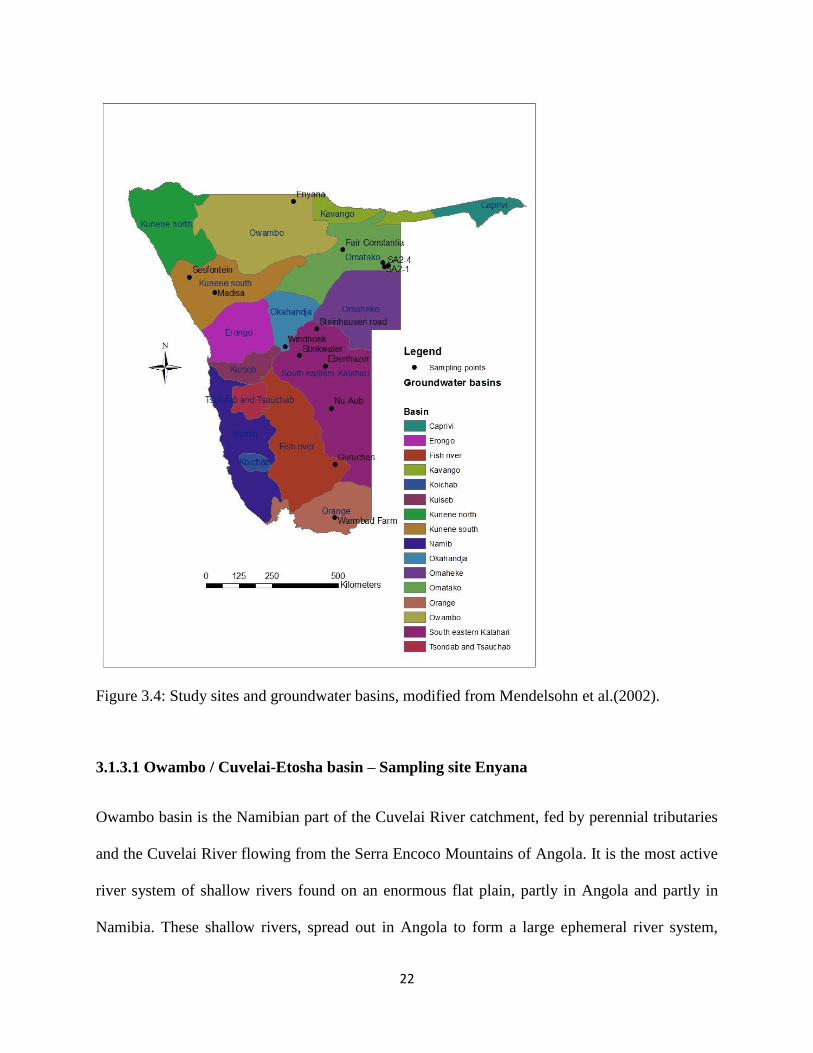
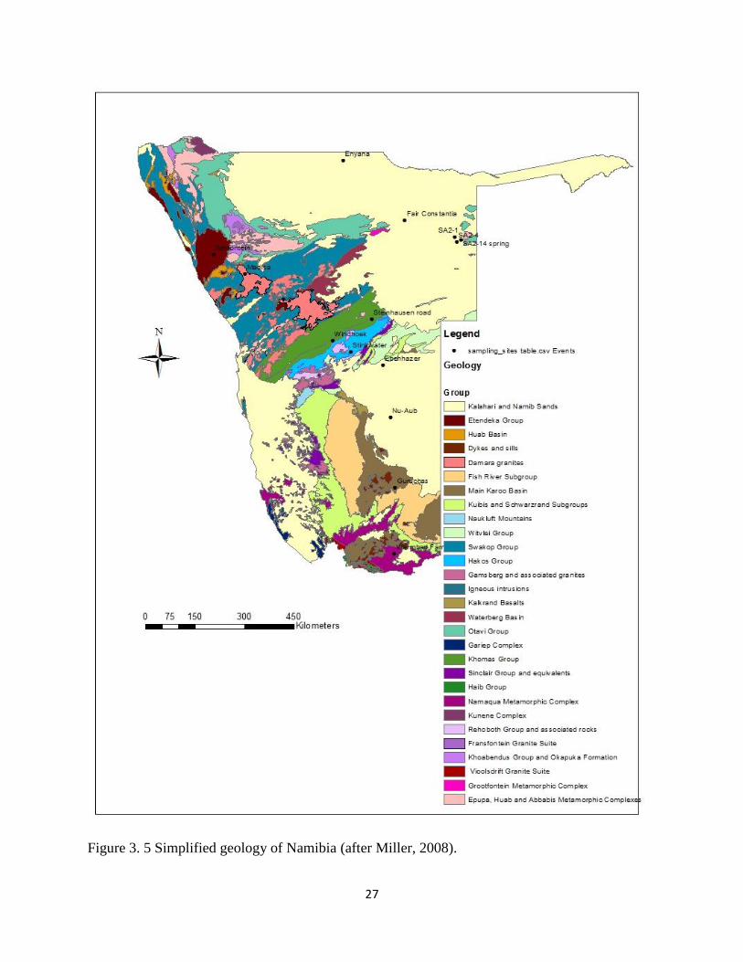
Namibia has been divided into sixteen groundwater basins based mainly on geological structure

and groundwater flow (Figure 3.9). Their boundaries were chosen to encompass areas of similar

geology and hydrogeology. The following aquifer systems exists in the country: fractured and

altered zones in the Archean basement, fractured rocks with a good proportion of limestones and

dolomites in Proterozoic Damara facies and Otavi series, porous rocks in Cambrian Nama

fromation and Post Cambrian formations and unconsolidated formations with good primary

porosity.

22

Figure 3.4: Study sites and groundwater basins, modified from Mendelsohn et al.(2002).

3.1.3.1 Owambo / Cuvelai-Etosha basin – Sampling site Enyana

Owambo basin is the Namibian part of the Cuvelai River catchment, fed by perennial tributaries

and the Cuvelai River flowing from the Serra Encoco Mountains of Angola. It is the most active

river system of shallow rivers found on an enormous flat plain, partly in Angola and partly in

Namibia. These shallow rivers, spread out in Angola to form a large ephemeral river system,

23

then come together in Namibia at Lake Oponono, which in turn drains into Etosha. The Etosha

basin is the outlet of the Cuvelai slopes. It was formed by faulting probably associated with the

Rift and the subsidence of the northern areas of Otavi facies (Christelis and Struckmeier, 2011).

Major groundwater recharge originates from Angola highland (Christelis and Struckmeier,

2011). The area is part of The Kalahari Sequence, entirely of continental aeolian to fluvial origin,

composed of Ombalantu, Beisib, Olukonda and Andoni formation. These formations are porous

and can absorb the surface flows and transmit them underground toward the areas where they

find their outlets. The groundwater aquifers are unconfined in the areas of recharge and

discharge, and artesian in the intermediate areas of groundwater flow.

The area is hosted in a multilayered aquifer system made up of one unconfined Perched

discontinuous Aquifer (PDA) and three confined continuous aquifers namely; Main shallow

aquifer (MSA), Main deep aquifer (MDA) and very deep aquifer (VDA). The Discontinuous

Perched Aquifer (DPA) is not a single aquifer, but consists of a series of small perched aquifers,

which occur predominantly in the dune-sand. These aquifers are mainly recharged by direct

infiltration of rainwater and exploited by means of traditional shallow hand dug wells. These

wells provide shallow, easily accessible and good quality drinking water to the villagers

(Christelis and Struckmeier, 2011).

3.1.3.2 Omatako basin - Sampling site Fair-Constansia

Groundwater within the area is hosted in two distinct aquifer systems, Kalahari aquifers and

fractured bedrock aquifers. Kalahari aquifers hold water in inter granular pore spaces, whereas

24

water in fractured aquifers is held in cracks and fractures in otherwise impermeable strata.

Shallow aquifers with water levels above 20m receive good recharge either directly from rainfall

or indirectly from ephemeral runoff. Deeper aquifers are recharged from the Kalahari basin

margins and under lying fractured aquifers. Groundwater level elevation (piezometric surface)

and hydro-chemical evidence suggest significant recharge from the Otavi Group dolomites in the

Tsumeb - Grootfontein area.

Boreholes closer to the center of the basin, tap deeper water as the depth to groundwater

gradually increases to more than 100 m. boreholes intersecting fractured bedrock aquifers may

show higher yields than boreholes tapping Kalahari aquifers. In areas of thin or absent Kalahari

cover lithological contacts and faults are discernible and borehole success rates are moderate.

Here, water quality is variable and saline groundwater can be expected in some boreholes. In the

bedrock areas adjacent to the Botswanan border water levels tend to be shallow although

groundwater levels can vary up to 10m in places between dry and wet seasons (Christelis and

Struckmeier, 2011).

3.1.3.3 South eastern Kalahari / Stampriet artesian basin - Sampling sites Nu-Aub,

Ebenhazer and Stinkwater

Groundwater occurs in the Nossob and Auob sandstones of the Ecca Group (lower Karoo

Sequence), which are divided by shale layers and overlain by Rietmond shale and sandstone.

Younger Kalkrand Basalt occurs in the north-west and Kalahari Sequence deposits.

Predominantly covered by Kalahari sediments: sands, clays, argillaceous, schists, calcareous

concretions and laterites. Several springs are located in the eastern outcrop area of the basalt.

25

The Karoo succession rests unconformably on Kamtsas Formation in the north and north-west

and on Nama Group rocks in the remainder of the basin. Sediment transport came from the

north-east. The sandstones, in particular, were deposited in a deltaic environment. The dip of the

Karoo formations is slightly towards the southeast and the groundwater flow generally follows

that direction.

Groundwater occurs in the Kalahari layers, in Kalkrand Basalt in the north-west, and in the

Prince Albert Formation of the Karoo Sequence. Elsewhere sub-artesian conditions prevail, that

is, the water in the aquifer is confined, but the pressure is not sufficient for the water to rise

above the surface. The artesian aquifers are recharged through sinkholes during years with

abnormally high rainfall.

3.1.3.4 Fish river Basin – Sampling site Guruchab

The area is composed of Fish River, Schwarzrand and the Kuibis subgroups of the Nama Group.

Groundwater is hosted in secondary features like faults and joints in sedimentary rocks of clastic

origin (sandstone, quartzite and shale) and in solution features in limestones and dolomites. Rock

types of the Nama Group are inherently impermeable with little or no primary porosity

3.1.3.5 Orange basin/ Karas basement - Sampling site Warmbad

Very limited volumes of groundwater are available in the basement rocks of the southern Karas

Region, since there are no productive aquifers due to lack recharge. The area has long been

inhabited, as the abundance of old hand-dug wells indicates. Most wells are situated along river

26

courses in shallow alluvium and deeply weathered channels and basins. Natural fountains occur

predominantly in riverbed. A thermal, fault controlled (±34° C) spring is found at Warmbad.

Exploration for groundwater should be concentrated along faults, and where possible close to

river beds, in order to facilitate and enhance recharge. The area is mainly underlain by granite-

gneiss of the Namaqualand Complex, along the riverbed it is deeply fractured and contains

highly mineralized water. Groundwater flow direction is north-west to south-east.

3.1.3.6 Okahandja basin/ central Namib – Sampling site Windhoek

Groundwater in Windhoek aquifer is recharged from rain water collecting along fractures in

quartzites of the Auas Mountains. Unsaturated zone storage is not always available due to rocky

terrain and shallow sand cover therefore component of rainfall that is not run- off rapidly

recharges the aquifer via preferred pathways. The rivers in this area are ephemeral and only flow

in thesummer rainy season. Windhoek is supplied water by the Omaruru and Swakop River. The

city was built around a series of natural springs, which occur close to the source of the Swakop

River.

27

Figure 3. 5 Simplified geology of Namibia (after Miller, 2008).

28

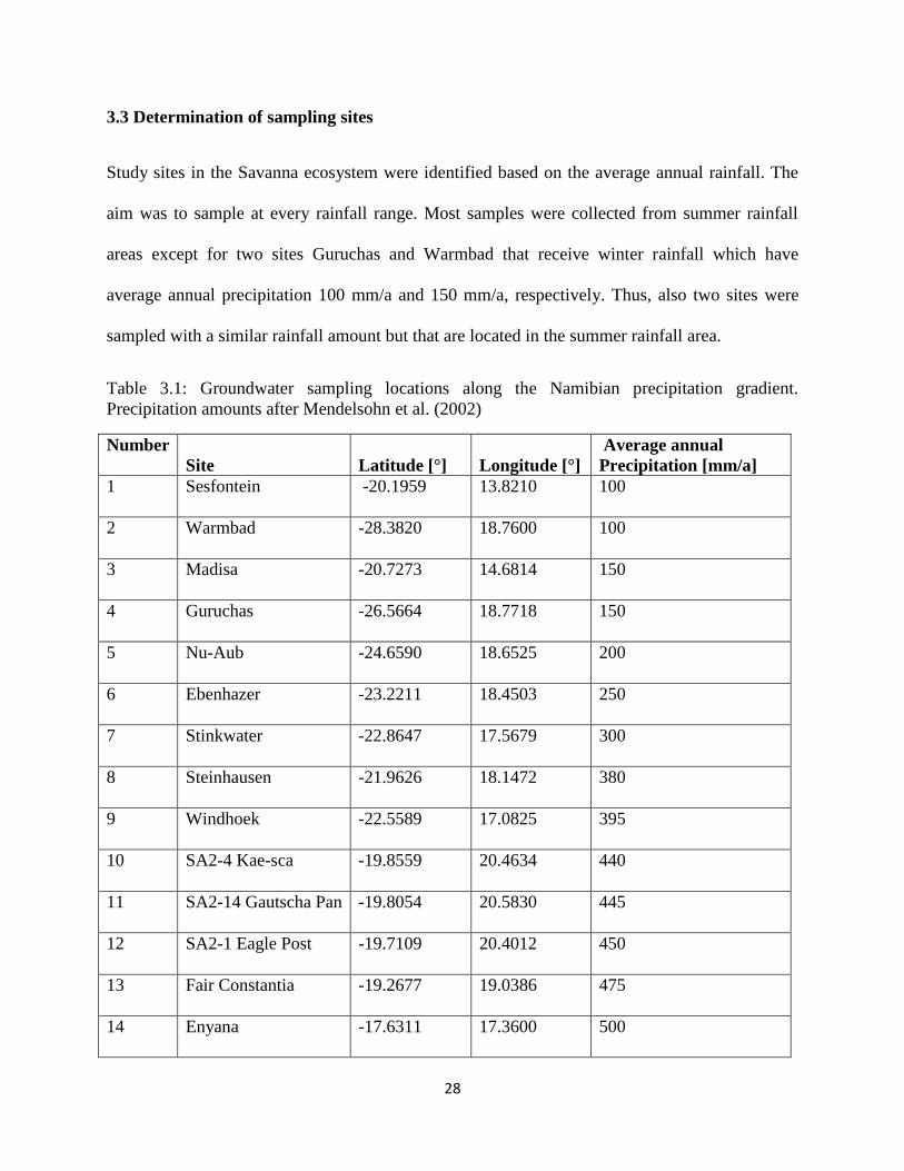
3.3 Determination of sampling sites

Study sites in the Savanna ecosystem were identified based on the average annual rainfall. The

aim was to sample at every rainfall range. Most samples were collected from summer rainfall

areas except for two sites Guruchas and Warmbad that receive winter rainfall which have

average annual precipitation 100 mm/a and 150 mm/a, respectively. Thus, also two sites were

sampled with a similar rainfall amount but that are located in the summer rainfall area.

Table 3.1: Groundwater sampling locations along the Namibian precipitation gradient.

Precipitation amounts after Mendelsohn et al. (2002)

Number

Site Latitude [°] Longitude [°]

Average annual

Precipitation [mm/a]

1 Sesfontein -20.1959 13.8210 100

2 Warmbad -28.3820 18.7600 100

3 Madisa -20.7273 14.6814 150

4 Guruchas -26.5664 18.7718 150

5 Nu-Aub -24.6590 18.6525 200

6 Ebenhazer -23.2211 18.4503 250

7 Stinkwater -22.8647 17.5679 300

8 Steinhausen -21.9626 18.1472 380

9 Windhoek -22.5589 17.0825 395

10 SA2-4 Kae-sca -19.8559 20.4634 440

11 SA2-14 Gautscha Pan -19.8054 20.5830 445

12 SA2-1 Eagle Post -19.7109 20.4012 450

13 Fair Constantia -19.2677 19.0386 475

14 Enyana -17.6311 17.3600 500

29

3.4. Study species

The following species were includes in the study: Vachellia erioloba/Acacia erioloba, Senegalia

mellifera/Acacia mellifera, Boscia albitrunca, Rhigozum trichotomum, Combretum imberbe,

Peltophorum africanum, P. juliflora, Terminalia sericea and Colophospermum mopane.

Table 3.2 Woody species sampling locations along the Namibian precipitation gradient.

No Site Species 1 Species 2 Species 3 Species 4

1 Sesfontein V. erioloba C. mopane B. albitrunca -

2 Warmbad V. erioloba R. tricotomum - -

3 Madisa V. erioloba C. mopane S. mellifera -

4 Guruchas V. erioloba R. trichotomum S. mellifera -

5 Nu-Aub V. erioloba R. trichotomum P. juliflora -

6 Ebenhazer V. erioloba S. mellifera B. albitrunca -

7 Stinkwater V. erioloba S. mellifera B. albitrunca -

8 Steinhausen V. erioloba T. sericea - -

9 Windhoek V. erioloba S. mellifera B. albitrunca A. Hebeclada

10 Fair

Constantia V. erioloba S. mellifera B. albitrunca -

11 Enyana V. erioloba S. mellifera C. imberbe P. Africanum

Woody tissue samples from SA2-1 Eagle post, SA2-14 Gautscha pan and SA2-4 Kae-sca were

not analysed for their isotopic composition due to high content of organic contaminants.

30

3.5 Data collection procedure

Plant sample from woody vegetation of the savanna ecosystem, groundwater and stream water

were collected randomly at all precipitation ranges. Woody tissue samples were taken from

mature, healthy appearing vegetation. These plants were correctly identified in the field with the

aid of Field’s guide to Trees and Shrubs of Namibia book by Mannheimer and Curtis (2009).

Xylem samples were collected using a xylem drill at approximately 1.4 m above the ground in

order to minimize contamination of xylem water with organic matter. The sampling spot is

freshly de-barked before drilling. Where the xylem drilling proved to be futile, twig segments

were opted for. Twigs less than one centimeter in diameter were cut from the tree with a pruning

shears. Leaves, thorns and loose barks are removed from the twig segments and cut into lengths

short enough to be placed into collection vials. Walker et al (2001) recommend removing of

leaves, bark from woody twigs before sampling as well as avoiding any green parts of a plant as

precautions to avoid mixing of xylem water with enriched, evaporated water from those parts. To

establish if there was a relationship between plant size and depth of water uptake, diameter at

breast height (DBH) was measured and height was estimated for every sampled tree/shrub.

Groundwater samples were collected from fourteen boreholes in close proximity to the sampled

plants. On-site parameters such as electrical conductivity and temperature were measured.

Further data for isotopic composition of groundwater in the area were obtained from Turewicz

(2013). Samples were stored at room temperature out of direct sunlight in screw-top glass and

plastic vials, sealed with parafilm in the field in order to avoid isotope fractionation due to

31

evaporation. Throughout the sampling campaign a total of 76 samples were collected, 14

groundwater samples, 20 twigs and 48 xylem drill samples.

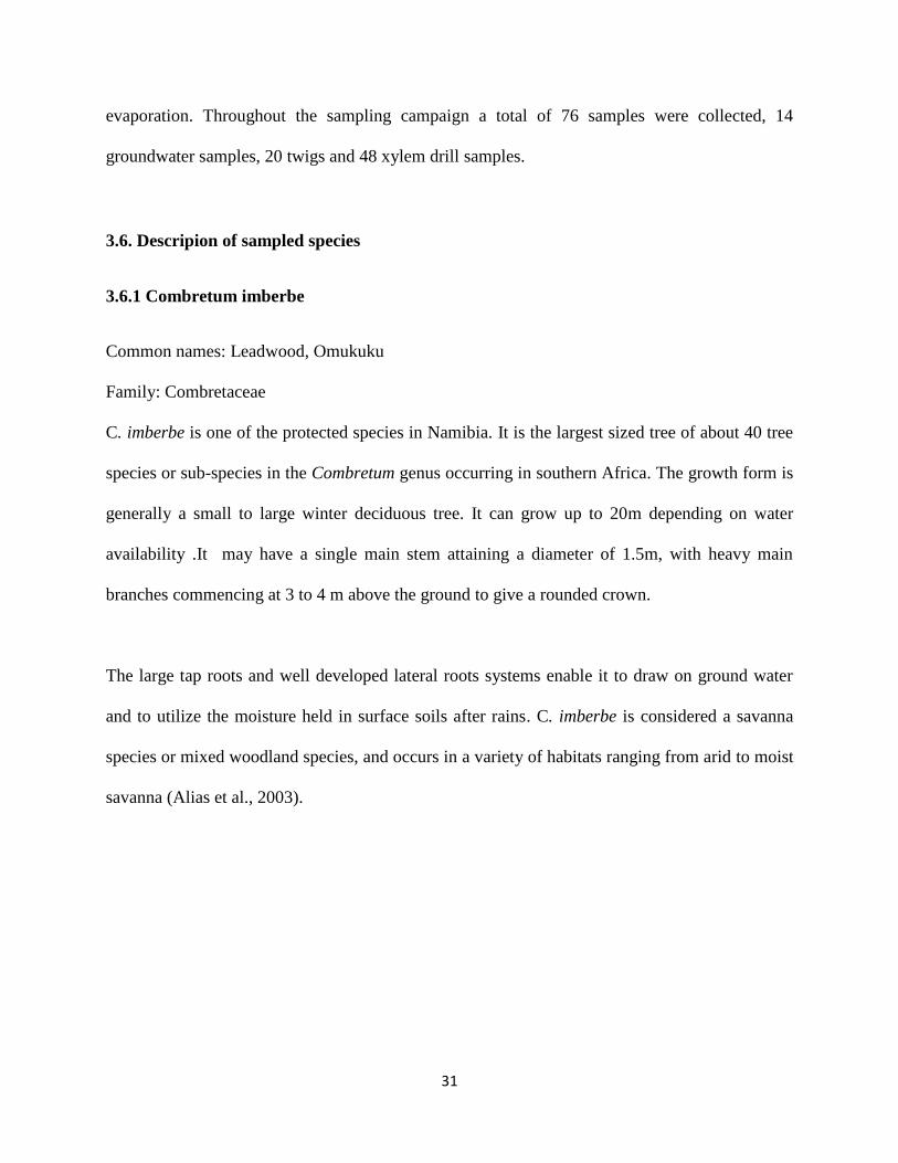
3.6. Descripion of sampled species

3.6.1 Combretum imberbe

Common names: Leadwood, Omukuku

Family: Combretaceae

C. imberbe is one of the protected species in Namibia. It is the largest sized tree of about 40 tree

species or sub-species in the Combretum genus occurring in southern Africa. The growth form is

generally a small to large winter deciduous tree. It can grow up to 20m depending on water

availability .It may have a single main stem attaining a diameter of 1.5m, with heavy main

branches commencing at 3 to 4 m above the ground to give a rounded crown.

The large tap roots and well developed lateral roots systems enable it to draw on ground water

and to utilize the moisture held in surface soils after rains. C. imberbe is considered a savanna

species or mixed woodland species, and occurs in a variety of habitats ranging from arid to moist

savanna (Alias et al., 2003).

32

Figure 3.6: Pale yellow Combretum imberbe tree to the right of a Mopane tree (b) Combretum

imberbe four-winged fruits.

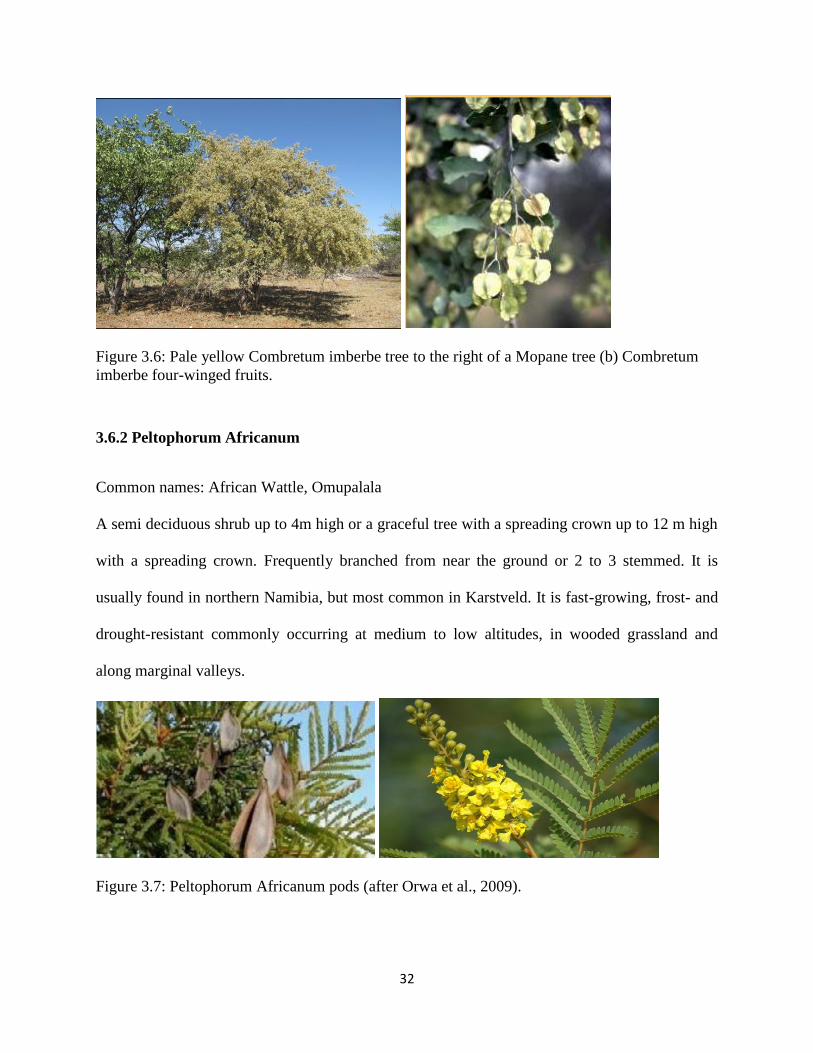
3.6.2 Peltophorum Africanum

Common names: African Wattle, Omupalala

A semi deciduous shrub up to 4m high or a graceful tree with a spreading crown up to 12 m high

with a spreading crown. Frequently branched from near the ground or 2 to 3 stemmed. It is

usually found in northern Namibia, but most common in Karstveld. It is fast-growing, frost- and

drought-resistant commonly occurring at medium to low altitudes, in wooded grassland and

along marginal valleys.

Figure 3.7: Peltophorum Africanum pods (after Orwa et al., 2009).

33

3.6.3 Acacia hebeclada

Common name: candle pod acacia, candle thorn

Family: Fabaceae

Acacia hebeclada has two distinct forms the subspecies hebeclada is a small shrub growing up to

1.5 metre tall, whilst the subspecies chobiensis is a large, thicket-forming shrub or small tree

growing up to 3 metres. Both forms branch from the ground, and occasionally form underground

stolons. (www.ville-ge.com). It is found in dry savanna and grassland areas and on soil ranging

from Kalahari sands to sandy alluvium soils, often associated with calcrete.

Figure 3.8: Acacia hebeclada shrub.

3.6.4 Vachalia erioloba / Acacia erioloba

Common names: Camel-thorn, omuthiya

Family: Fabaceae

Vachalia erioloba is the common and widely distributed woody species throughout the entire

country. It is a semi-deciduous tree; its stature varies from a shrub to a very large tree with a

spreading crown, depending upon water availability and depth. This species can grow up to 30 m

34

high, trunk circumference up to 4 m. Vachalia erioloba prefers sandy soil, depressions and dry

riverbeds. Tap roots can grow up to 60 m deep (Jennings 1974)

Figure 3.9: Vachallia erioloba tree.

3.6.5 Senegalia mellifera/ Acacia mellifera

Common names : Wait a bit thorn, black thorn, hook thorn

Acacia mellifera is a low, branched tree with a more or less spherical crown. It has a shallow but

extensive root system radiating from the crown, allowing the plant to exploit soil moisture and

nutrients from a large volume of soil. The roots rarely penetrate more than 1 m. A. mellifera is a

commonly occurring shrub on rangelands throughout the savanna. A. mellifera is normally found

on hard-surfaced, sandy soils and rocky hillsides. This species is drought-tolerant; it grows well

on most soil types but prefers loamy soils with mean annual rainfall of 250-700 mm (Orwa et al.,

2009).

35

Figure 3.10: Senegallia mellifera shrub.

3.6.6 Boscia albitrunca

Common names: Shepherd tree, Omunghudi

Family: Capparaceae

Boscia albitrunca is als a protected species in Namibia. It is a stocky evergreen tree that may

reach heights of 5-11 m , it usually has a well rounded crown . It prefers to grow on sandy,

loamy and calcrete soils . Matured B. albitrunca trees has been found to be among the most

drought torelant species (Alias et al., 2003). In the savanna ecosystem maximum rooting depth is

0.5 ± 0.1, however in the central Kalahari 68 m rooting depth was encountered (Obakeng, 2007)

Figure 3.11: Boscia Albitrunca tree.

36

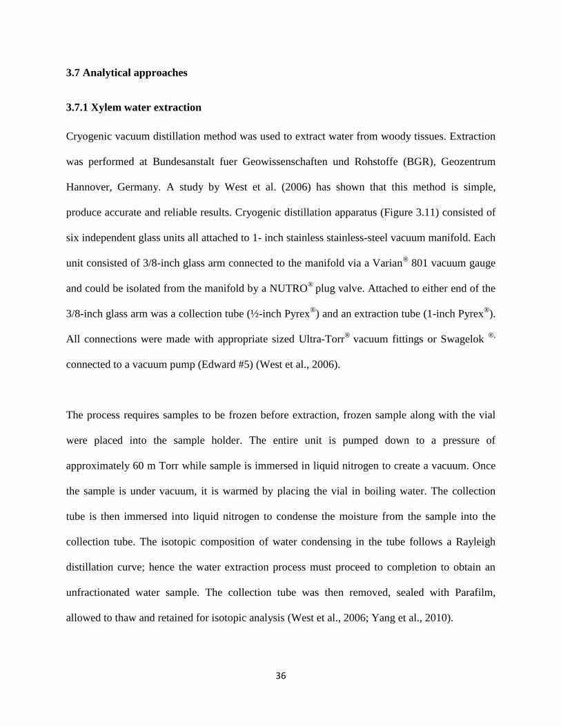
3.7 Analytical approaches

3.7.1 Xylem water extraction

Cryogenic vacuum distillation method was used to extract water from woody tissues. Extraction

was performed at Bundesanstalt fuer Geowissenschaften und Rohstoffe (BGR), Geozentrum

Hannover, Germany. A study by West et al. (2006) has shown that this method is simple,

produce accurate and reliable results. Cryogenic distillation apparatus (Figure 3.11) consisted of

six independent glass units all attached to 1- inch stainless stainless-steel vacuum manifold. Each

unit consisted of 3/8-inch glass arm connected to the manifold via a Varian® 801 vacuum gauge

and could be isolated from the manifold by a NUTRO®

plug valve. Attached to either end of the

3/8-inch glass arm was a collection tube (½-inch Pyrex®

) and an extraction tube (1-inch Pyrex®).

All connections were made with appropriate sized Ultra-Torr®

vacuum fittings or Swagelok ®,

connected to a vacuum pump (Edward #5) (West et al., 2006).

The process requires samples to be frozen before extraction, frozen sample along with the vial

were placed into the sample holder. The entire unit is pumped down to a pressure of

approximately 60 m Torr while sample is immersed in liquid nitrogen to create a vacuum. Once

the sample is under vacuum, it is warmed by placing the vial in boiling water. The collection

tube is then immersed into liquid nitrogen to condense the moisture from the sample into the

collection tube. The isotopic composition of water condensing in the tube follows a Rayleigh

distillation curve; hence the water extraction process must proceed to completion to obtain an

unfractionated water sample. The collection tube was then removed, sealed with Parafilm,

allowed to thaw and retained for isotopic analysis (West et al., 2006; Yang et al., 2010).

37

Figure 3.12: Cryogenic extraction line (after West et al., 2006).

3.7.2 Analysis of hydrogen and oxygen isotopic ratios

Obtained water samples were analyzed for their isotopic composition using isotope ratio infrared

spectrometer (L2120-i wavelength-scanned cavity ring-down spectrometer, Picarro Inc.) at the

same laboratory. This device uses a Wavelength-Scanned Cavity Ringdown Spectroscopy (WS-

CRDS) measure the absorption line features for three common water isotopologues: 1H2

16O,

HD16

O and 1H2

18O (Bailey et al., 2015).

Infrared laser spectroscopy has gained popularity in the recent years due to its time efficiency

since no extensive sample preparation is required. The analyzer has three components

38

(Figure3.12) a gas-phase instrument that measures the concentration and isotopic content of

water in vapor form, a liquid evaporator that homogeneously vaporizes liquid water with little or

no isotopic fractionation and an auto-sampler that injects liquid water samples into the

evaporator. Vaporization enables the WS-CRDS cavity to be loaded with a higher vapor pressure

to increasing the level of sensitivity and precision.

Figure 3.13: Major components of Isotope Ratio Infrared Spectrometer (L2120-i WS-CRDS) A:

PAL auto-sampler, B: Picarro vaporizer, C: Picarro analyzer.

Figure 3.14: (a) Schematic of Picarro CRDS analyzer showing how a ring down measurement is

carried out. (b) Demonstration on how optical loss is rendered into a time measurement (source:

www.picarro.com).

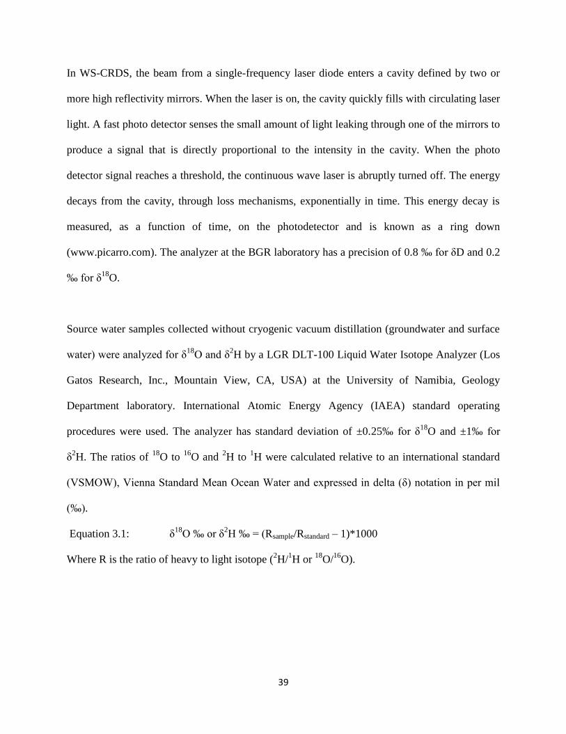
39

In WS-CRDS, the beam from a single-frequency laser diode enters a cavity defined by two or

more high reflectivity mirrors. When the laser is on, the cavity quickly fills with circulating laser

light. A fast photo detector senses the small amount of light leaking through one of the mirrors to

produce a signal that is directly proportional to the intensity in the cavity. When the photo

detector signal reaches a threshold, the continuous wave laser is abruptly turned off. The energy

decays from the cavity, through loss mechanisms, exponentially in time. This energy decay is

measured, as a function of time, on the photodetector and is known as a ring down

(www.picarro.com). The analyzer at the BGR laboratory has a precision of 0.8 ‰ for δD and 0.2

‰ for δ18

O.

Source water samples collected without cryogenic vacuum distillation (groundwater and surface

water) were analyzed for δ18

O and δ2H by a LGR DLT-100 Liquid Water Isotope Analyzer (Los

Gatos Research, Inc., Mountain View, CA, USA) at the University of Namibia, Geology

Department laboratory. International Atomic Energy Agency (IAEA) standard operating

procedures were used. The analyzer has standard deviation of ±0.25‰ for δ18

O and ±1‰ for

δ2H. The ratios of

18O to

16O and

2H to

1H were calculated relative to an international standard

(VSMOW), Vienna Standard Mean Ocean Water and expressed in delta (δ) notation in per mil

(‰).

Equation 3.1: δ18

O ‰ or δ2H ‰ = (Rsample/Rstandard – 1)*1000

Where R is the ratio of heavy to light isotope (2H/

1H or

18O/

16O).

40

3.7.3 Isotopic correction of xylem water

Results obtained from analysis were subjected to ChemCorrect™, Picarro’s post-processing

software package. It identifies and flags contamination from a broad range of organics, providing

confidence in the accuracy of isotope ratios reported. However, organic contaminants in isotope

analyses of xylem water with spectroanalyses and possible interferences are on-goingly

discussed in the research community and more research is still needed to assess their final

reliability.

3.8 Statistical analysis

All statistical analyses were performed using XLSTAT 2016. A linear model test was used

deduce the relationship between δ18

O and δ2H of groundwater and tree xylem water with

reference to GMWL. It was also used to infer the relationship between Diameter at Breast Height

(DBH) and groundwater isotopic composition as well as to test the relationship between isotopic

compositions of sampled groundwater to groundwater database.

Analysis of variance (ANOVA) was used to assess variability of isotopic composition of

groundwater and xylem waters. Such an approach was revealed useful to discriminate the

importance of ecological factors influencing water uses. Posterior Turkey’s test was used for

multiple comparisons in order to determine the significant differences between local

groundwater and xylem water. The P-values were considered statistically significant at the 0.05

level.

41

3.9 Tracing the isotopic composition of precipitation

Isotopic composition of groundwater in arid regions can be considerably modified from that of

local precipitation and vice versa. The evaporation slope for δ18

O and δ2H is a function of

humidity and vary between 4 and 5. Therefore the characteristic trends imparted by evaporation

can be useful in understanding mechanism of recharge as well as determining recharge rates,

which can be as low as or lower than 1% of precipitation. Despite the strong evaporation in arid

regions, it is possible that newly formed groundwater can have isotope contents close to the

mean composition of precipitation (Clark and Fritz, 1997).

The isotopic composition of precipitation where groundwater originated was traced by

calculating the intersection points of local groundwater evaporation lines with Global Meteoric

Water Line (GMWL) the precipitation source value (Evaristo et al. 2015) using the equation

below.

Equation 3.2: b = δ2H - (4.5 * δ

18O)

Equation 3.3: δ2H intercept = δ

2H – m δ

18O

= (δ18

O *8) + 10

Equation 3.4: δ18

O intercept = (δ2H intercept -b)/a

= (b- 10)/3.5

Where m, a and b are the slope of evaporation line (4 to 5 for arid regions), the GMWL slope,

and the GMWL intercept, respectively. The same equation was used trace the source of

groundwater recharge at Guruchas - the only site where surface water was encountered

presumably from recent rainfall.

42

CHAPTER 4

4. Results

4.1 Isotopic composition of water available for plant uptake

Groundwater Oxygen and Hydrogen isotope ratios analyzed throughout the study varied

depending on location. These values were plotted together with isotope database compiled by

Turewicz (2013) to characterize groundwater recharge. Groundwater samples from Guruchab,

SA2-14 and Steinhausen displayed very high levels of enrichment in comparison to groundwater

samples from other locations.

Guruchab sampled groundwater had δ18

O and δD composition of -4.08‰ and -30.5‰; it plotted

below the GMWL along an evaporation line (Figure 4.1(a)), while groundwater database δ18

O

and δD composition varied from -6.57‰ to -2.15‰ (mean: -4.30 ± 1.1‰) and -42.43‰ to -

21.51‰ (mean: -31.35 ± 5.3‰). Steinhausen Sampled groundwater had δ18

O and δD

composition of -5.04‰ and -38.8‰ (Figure 4.1(b)) slightly enriched than groundwater database

which varied from -7.44‰ to -5.04‰ (mean -6.66 ± 1.10‰) and -53.20‰ to -38.85‰ (mean: -

48.76 ± 6.72‰).

43

Figure 4.1: Groundwater δ18

O and δD composition for (a) Guruchab and (b) Steinhausen.

Ebenhazer sampled groundwater had δ18

O and δD composition of -7.22‰ and -53.6‰ (Figure

4.2 (a)). It was within the range of groundwater database which varied from -7.9‰ to -4.8‰

(mean -6.82 ± 0.8‰) and -56.0‰ to -41.0‰ (mean: -49.58 ± 3.9‰). Sampled groundwater from

Stinkwater plotted along the GMWL and the groundwater database δ18

O and δD composition

varied from -9.27‰ to -6.19‰ (mean -7.82 ± 1.5‰) and -60.72‰ to -42.49‰ (mean: -50.33 ±

8.5‰) (Figure 4.2(b)).

GMWL

-80

-60

-40

-20

0

-10 -5 0

δD

(‰

V-S

MO

W)

δ18O (‰ V-SMOW)

(a)Guruchab

Groundwater database

Guruchab

GMWL

-80

-60

-40

-20

0

-10 -5 0

δD

(‰

V-S

MO

W)

δ18O (‰ V-SMOW)

(b) Steinhausen road

Groundwater database Steinhousen road

44

Figure 4.2: Groundwater δ18

O and δD composition for (a) Ebenhazer and (b) Stinkwater.

Warmbad sampled groundwater had δ18

O and δD composition of -5.69‰ and -88.5‰; it plotted

above the GMWL presumably due to mixing with recent rainfall or a deviating of the LMWL

from the GMWL (Figure 4.3(a)), while groundwater database composition varied from -6.79‰

to -2.15‰ (mean -5.17 ± 1.6‰) and -43.68‰ to -18.72‰ (mean: -34.57 ± 7.9‰). Madisa

groundwater had the same δ18

O as Warmbad, but different deuterium excess, d excess = 2.24‰

and -42.45‰ for Madisa and Warmbad, respectively. Madisa sampled groundwater had δ18

O and

δD composition of -5.53‰ and -42.0‰ (Figure 4.3(b)). It was within the range of groundwater

database which varied from -9.70‰ to -3.73‰ (mean -5.67 ± 1.8‰) and -68.50‰ to -29.10‰

(mean: -40. 06 ± 12.1‰).

GMWL

-80

-60

-40

-20

0

-10 -8 -6 -4 -2 0

δD

(‰

V-S

MO

W)

δ18O (‰ V-SMOW)

(a) Ebenhazer

Groundwater database Ebenhazer

GMWL

-80

-60

-40

-20

0

-10 -5 0

δD

(‰

V-S

MO

W)

(b) Stinkwater

Groundwater database Stinkwater

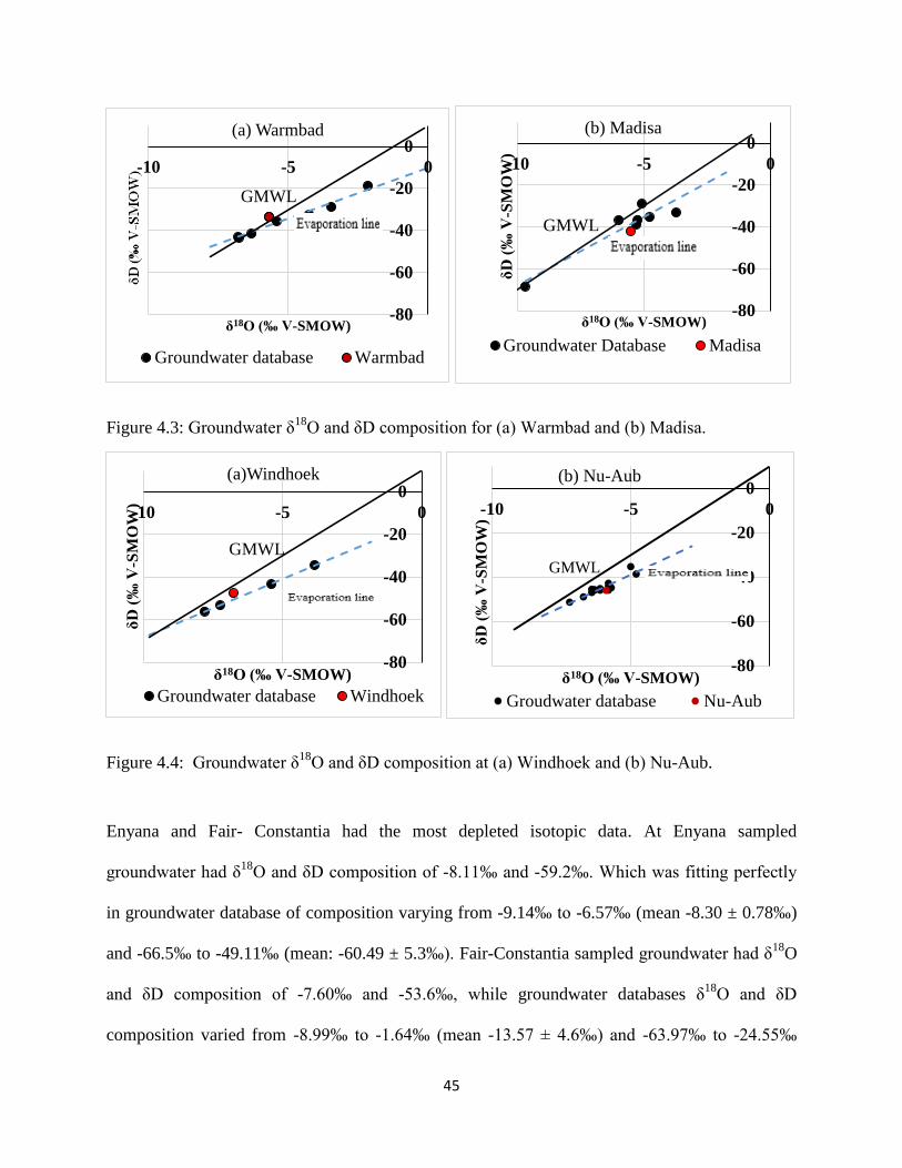
45

Figure 4.3: Groundwater δ18

O and δD composition for (a) Warmbad and (b) Madisa.

Figure 4.4: Groundwater δ18

O and δD composition at (a) Windhoek and (b) Nu-Aub.

Enyana and Fair- Constantia had the most depleted isotopic data. At Enyana sampled

groundwater had δ18

O and δD composition of -8.11‰ and -59.2‰. Which was fitting perfectly

in groundwater database of composition varying from -9.14‰ to -6.57‰ (mean -8.30 ± 0.78‰)

and -66.5‰ to -49.11‰ (mean: -60.49 ± 5.3‰). Fair-Constantia sampled groundwater had δ18

O

and δD composition of -7.60‰ and -53.6‰, while groundwater databases δ18

O and δD

composition varied from -8.99‰ to -1.64‰ (mean -13.57 ± 4.6‰) and -63.97‰ to -24.55‰

GMWL

-80

-60

-40

-20

0

-10 -5 0

δ18O (‰ V-SMOW)

(a) Warmbad

Groundwater database Warmbad

GMWL

-80

-60

-40

-20

0

-10 -5 0

δD

(‰

V-S

MO

W)

δ18O (‰ V-SMOW)

(b) Madisa

Groundwater Database Madisa

GMWL

-80

-60

-40

-20

0

-10 -5 0

δD

(‰

V-S

MO

W)

δ18O (‰ V-SMOW)

(a)Windhoek

Groundwater database Windhoek

GMWL

-80

-60

-40

-20

0

-10 -5 0

δD

(‰

V-S

MO

W)

δ18O (‰ V-SMOW)

(b) Nu-Aub

Groudwater database Nu-Aub

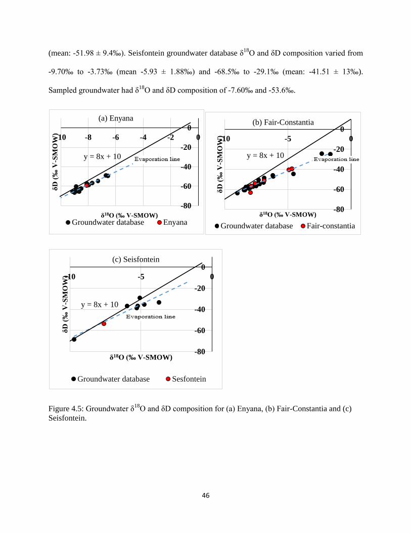
46

(mean: -51.98 ± 9.4‰). Seisfontein groundwater database δ18

O and δD composition varied from

-9.70‰ to -3.73‰ (mean -5.93 ± 1.88‰) and -68.5‰ to -29.1‰ (mean: -41.51 ± 13‰).

Sampled groundwater had δ18

O and δD composition of -7.60‰ and -53.6‰.

Figure 4.5: Groundwater δ18

O and δD composition for (a) Enyana, (b) Fair-Constantia and (c)

Seisfontein.

y = 8x + 10

-80

-60

-40

-20

0

-10 -8 -6 -4 -2 0

δD

(‰

V-S

MO

W)

δ18O (‰ V-SMOW)

(a) Enyana

Groundwater database Enyana

y = 8x + 10

-80

-60

-40

-20

0

-10 -5 0

δD

(‰

V-S

MO

W)

δ18O (‰ V-SMOW)

(b) Fair-Constantia

Groundwater database Fair-constantia

y = 8x + 10

-80

-60

-40

-20

0

-10 -5 0

δD

(‰

V-S

MO

W)

δ18O (‰ V-SMOW)

(c) Seisfontein

Groundwater database Sesfontein

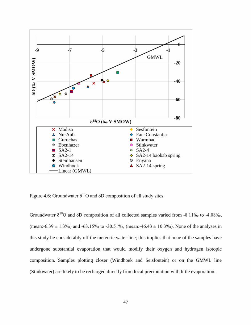
47

Figure 4.6: Groundwater δ18

O and δD composition of all study sites.

Groundwater δ18

O and δD composition of all collected samples varied from -8.11‰ to -4.08‰,

(mean:-6.39 ± 1.3‰) and -63.15‰ to -30.51‰, (mean:-46.43 ± 10.3‰). None of the analyses in

this study lie considerably off the meteoric water line; this implies that none of the samples have

undergone substantial evaporation that would modify their oxygen and hydrogen isotopic

composition. Samples plotting closer (Windhoek and Seisfontein) or on the GMWL line

(Stinkwater) are likely to be recharged directly from local precipitation with little evaporation.

GMWL

-80

-60

-40

-20

0

-9 -7 -5 -3 -1

δD

(‰

V-S

MO

W)

δ18O (‰ V-SMOW)

Madisa SesfonteinNu-Aub Fair-ConstantiaGuruchas WarmbadEbenhazer StinkwaterSA2-1 SA2-4SA2-14 SA2-14 baobab springSteinhausen EnyanaWindhoek SA2-14 springLinear (GMWL)

48

All groundwater samples fall below the Global Meteoric Water Line (GMWL), except for

Warmbad. The deviation from the GMWL is due to evaporation process, typical of semi-arid to

arid climatic conditions. Groundwater samples from the north part of the country were more

depleted in heavy isotopes, while samples from the southern part were least depleted/ enriched in

heavy isotopes.

Model calculation has shown that groundwater from Guruchab was recharged from precipitation

with δ2H and δ

18O values of -6.3‰ and -40.6‰, respectively. This shows that the standing water

from Guruchab must has been around for quite some time to have attained such enriched

composition of -0.07‰ and -11.8‰ for δ18

O and δD.

4.2 Isotopic composition of precipitation

Isotopic composition of precipitation where groundwater originated was traced by calculating the

intersection points of local groundwater evaporation lines with GMWL.

Table 4.1: δ18

O and δD composition of groundwater, deuterium excess and isotopic composition

of recalculated precipitation.

Site Groundwater

δ18

O (‰)

Groundwater

δD(‰)

d-excess(‰) Precipitation

δ18

O

Precipitation

δD

SA2-14 -4.68 -39.3 -1.9 -8.1 -54.7

Fair

Constantia

-7.95 -63.1 0.4 -10.7 -75.4

Nu-Aub -5.89 -46.1 1 -8.4 -57.6

Steinhausen -5.04 -38.8 1.4 -7.5 -49.8

Guruchab -4.08 -30.5 2.1 -6.3 -40.6

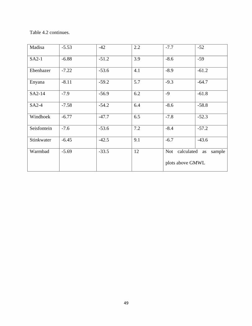
49

Table 4.2 continues.

Madisa -5.53 -42 2.2 -7.7 -52

SA2-1 -6.88 -51.2 3.9 -8.6 -59

Ebenhazer -7.22 -53.6 4.1 -8.9 -61.2

Enyana -8.11 -59.2 5.7 -9.3 -64.7

SA2-14 -7.9 -56.9 6.2 -9 -61.8

SA2-4 -7.58 -54.2 6.4 -8.6 -58.8

Windhoek -6.77 -47.7 6.5 -7.8 -52.3

Seisfontein -7.6 -53.6 7.2 -8.4 -57.2

Stinkwater -6.45 -42.5 9.1 -6.7 -43.6

Warmbad -5.69 -33.5 12 Not calculated as sample

plots above GMWL

50

Figure 4.7: Groundwater (blue squares) and calculated source precipitation δD and δ18

O

compositions with reference to GMWL. Samples from the north east (Fair Constantia and

Enyana) have the most depleted source water. While samples from the southern part have more

enriched source water.

GMWL

-80

-60

-40

-20

0

-12 -10 -8 -6 -4 -2 0

Madisa Seisfontein Fair Constantia

Nu-Aub Guruchas Stinkwater

SA2-1 SA2-4 SA2-14

SA2-14 baobab spring Steinhausen Enyana

Windhoek

51

4.3 Precipitation isotopic variation

4.3.1 Latitude effect

A strong negative correlation (R2=0.64) existed between calculated δ

18O of precipitation and

latitude and it is statistically insignificant (P>0.05). The observed gradient over the entire

country was approximately -0.37‰ per degree latitude for δ18

O.

Figure 4.8: The relationship between latitude and precipitation δ18

O values of all the sampling

points.

4.3.2 Longitude

The correlation between longitude and δ18

O composition of precipitation was very weak

(R2=0.016) and statistically insignificant (P>0.05). The observed longitude effect was

approximately 0.09‰ δ18

O per degree longitude.

y = -0.3713x - 16.223

R² = 0.6432

-12

-9

-6

-3

-30 -25 -20

δ1

8O

(‰

V-S

MO

W)

Latitude (o)

52

Figure 4.9: The relationship between longitude and precipitation δ18

O values of all the sampling

points.

4.3.3 Distance from the coast

The correlation between distance from the coast and δ18

O composition of precipitation was

negatively and weak (R2=0.29) and statistically significant (P<0.05). A relationship between

δ18

O in precipitation and its distance from the coast was found with an estimated depletion rate

of -0.31 ‰ in precipitation per 100 km inland.

y = -0.0879x - 6.4777

R² = 0.0157

-12

-9

-6

-3

12 15 18 21δ

18O

(‰

V-S

MO

W)

Longitude (o)

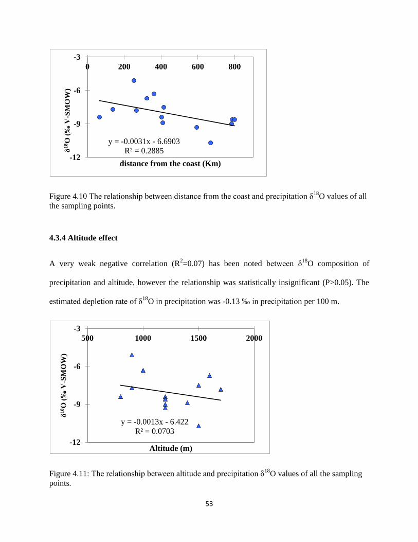
53

Figure 4.10 The relationship between distance from the coast and precipitation δ18

O values of all

the sampling points.

4.3.4 Altitude effect

A very weak negative correlation (R2=0.07) has been noted between δ

18O composition of

precipitation and altitude, however the relationship was statistically insignificant (P>0.05). The

estimated depletion rate of δ18

O in precipitation was -0.13 ‰ in precipitation per 100 m.

Figure 4.11: The relationship between altitude and precipitation δ18

O values of all the sampling

points.

y = -0.0031x - 6.6903

R² = 0.2885 -12

-9

-6

-3

0 200 400 600 800δ

18O

(‰

V-S

MO

W)

distance from the coast (Km)

y = -0.0013x - 6.422

R² = 0.0703

-12

-9

-6

-3

500 1000 1500 2000

δ1

8O

(‰

V-S

MO

W)

Altitude (m)

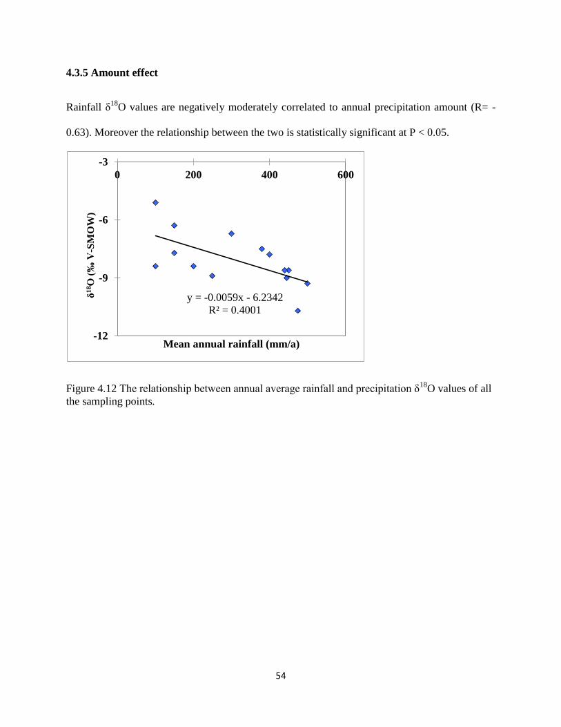
54

4.3.5 Amount effect

Rainfall δ18

O values are negatively moderately correlated to annual precipitation amount (R= -

0.63). Moreover the relationship between the two is statistically significant at P < 0.05.

Figure 4.12 The relationship between annual average rainfall and precipitation δ18

O values of all

the sampling points.

y = -0.0059x - 6.2342

R² = 0.4001

-12

-9

-6

-3

0 200 400 600

δ1

8O

(‰

V-S

MO

W)

Mean annual rainfall (mm/a)

55

4.4 Isotopic composition of woody vegetation xylem water

4.4.1 Madisa

-120

-80

-40

0

-16 -12 -8 -4 0

(a)Madisa

Colophospermum mopane Vachellia erioloba

Senegalia mellifera Groundwater

Groundwater Database Linear (GMWL)

R² = 0.7885

-90

-60

-30

0

-10 -5 0

AX

IS T

ITLE

AXIS TITLE

(b) C. mopane

R² = 0.9317

-120

-80

-40

0

-15 -12 -9 -6 -3 0

AX

IS T

ITLE

AXIS TITLE

(c ) V .er io loba

56

Figure 4.13: Woody vegetation xylem water and groundwater δD and δ18

O compositions with

reference to GMWL. Linear correlation between groundwater and (b) C. mopane, (b) V.erioloba,

(d) S. mellifera at Madisa.

At Madisa, the isotopic composition of the woody vegetation is more negative than groundwater.

The δ18

O and δD value of V. erioloba xylem water was found to be -13.96‰ and -114.3‰,

respectively. While, C. mopane xylem water δ18

O and δD values were -8.81‰ and -76.7‰,

respectively. These values were lesser than those obtained from S. mellifera which were recorded

as -6.72‰ and 81.2‰ for δ18

O and δD respectively. S. mellifera was transpiring water with

slightly similar δ18

O composition as local groundwater but highly depleted in δD.

The plot of the xylem water together with groundwater indicate that S. mellifera was utilizing

groundwater while V. erioloba and C. mopane were utilizing slightly depleted soil water

probably recharged by heavy rainfall some months earlier.

R² = 0.4634

-90

-60

-30

0

-10 -8 -6 -4 -2 0

AX

IS T

ITLE

AXIS TITLE

(d) S .mel l i fe ra

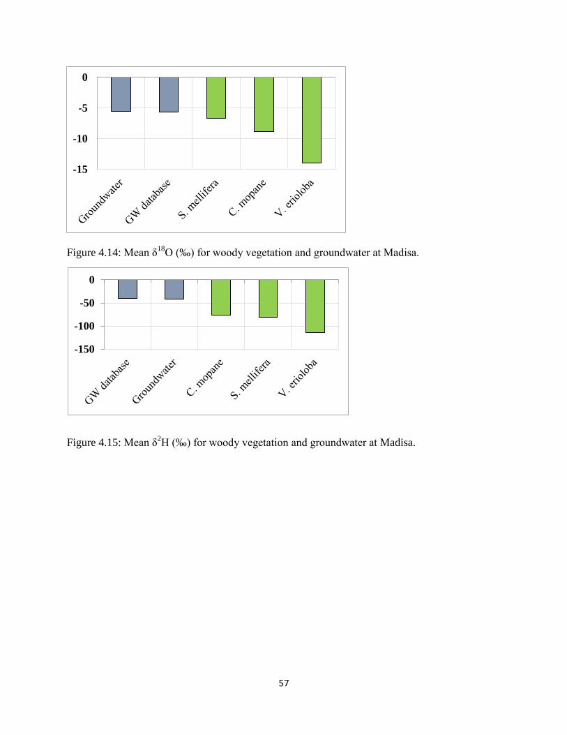
57

Figure 4.14: Mean δ18

O (‰) for woody vegetation and groundwater at Madisa.

Figure 4.15: Mean δ2H (‰) for woody vegetation and groundwater at Madisa.

-15

-10

-5

0

-150

-100

-50

0

58

4.4.2 Seisfontein

-100

-80

-60

-40

-20

0

20

-1 0 -8 -6 -4 -2 0 2

(a) Se is fontein

Groundwater Colophospermum mopane

Vachellia erioloba Boscia albitrunca

R² = 0.7993

-80

-60

-40

-20

0

-1 2 -8 -4 0

AX

IS T

ITLE

AXIS TITLE

(b) B. a lb i t runca

R² = 0.7985

-80

-60

-40

-20

0

-1 2 -8 -4 0

AX

IS T

ITLE

AXIS TITLE

(c ) C. mopane

59

Figure 4.16: (a) Woody vegetation xylem water and groundwater δ2H and δ

18O compositions

with reference to GMWL. A biplot of δ18

O – δ2H showing regression relationship between

groundwater (b) B. albitrunca, (c) C.mopane and (d) V. erioloba at Seisfontein.

Groundwater plotted along the GMWL unlike woody species xylem water which all deviated

from the GMWL. C. mopane and B. albitrunca xylem water had isotopic composition similar to

groundwater. C. mopane xylem water δ18

O and δD composition was -6.99‰ and 64.2‰,

respectively. This was slightly similar to B. albitrunca, which was 6.48‰ and 59.2‰.

Meanwhile V. erioloba xylem water was the most depleted, isotopic composition was -9.41‰

and - 94.7‰, for δ18

O and δD respectively, but was still within the groundwater database range.

From the analysis of δ18

O and δD data, all sampled species appear to have been using

groundwater in the same range as groundwater database, but slightly depleted in δD.

R² = 0.8297

-100

-80

-60

-40

-20

0

-1 2 -8 -4 0

AX

IS T

ITLE

AXIS TITLE

(d ) V . e r io loba

60

Figure 4.17: Mean δ18

O (‰) for woody vegetation and groundwater at Seisfontein.

Figure 4.18: Mean δ2H (‰) for woody vegetation and groundwater at Seisfontein.

-12

-8

-4

0

-100

-75

-50

-25

0

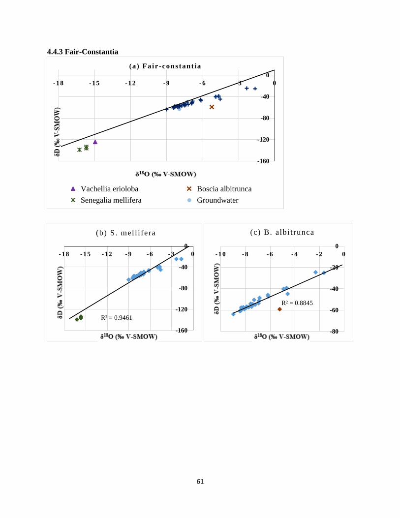
61

4.4.3 Fair-Constantia

-160

-120

-80

-40

0

-1 8 -1 5 -1 2 -9 -6 -3 0

(a) Fair -constant ia

Vachellia erioloba Boscia albitrunca

Senegalia mellifera Groundwater

R² = 0.9461

-160

-120

-80

-40

0

-1 8 -1 5 -1 2 -9 -6 -3 0

(b) S . mel l i fera

R² = 0.8845

-80

-60

-40

-20

0

-1 0 -8 -6 -4 -2 0

(c) B. albi t runca

62

Figure 4.19: Figure 4.19 (a) Woody vegetation xylem water and groundwater δ2H and δ18O

compositions with reference to GMWL. A biplot of δ18

O – δ2H showing regression relationship

between groundwater and (b) S.mellifera, (c) B.albitrunca and (d) V. erioloba at Fair Constantia.

At this study site xylem water isotope composition for S. mellifera was the most depleted,

followed by V. erioloba. Moreover B. albitrunca xylem isotope composition was similar to local

groundwater. This confirms that B. albitrunca was utilizing groundwater while V erioloba and S.

mellifera were utilizing soil water.

Figure 4.20: Mean δ18

O (‰) for woody vegetation and groundwater at Fair-Constantia.

R² = 0.9251

-150

-120

-90

-60

-30

0

-1 6 - 1 2 -8 -4 0

(d) V. er ioloba

-20

-15

-10

-5

0

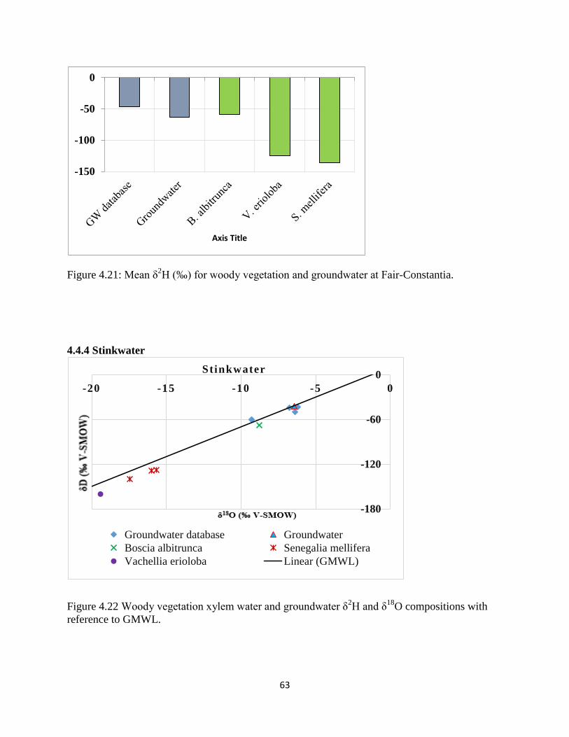
63

Figure 4.21: Mean δ2H (‰) for woody vegetation and groundwater at Fair-Constantia.

4.4.4 Stinkwater

Figure 4.22 Woody vegetation xylem water and groundwater δ2H and δ

18O compositions with

reference to GMWL.

-150

-100

-50

0

Axis Title

-180

-120

-60

0

-20 -15 -10 -5 0

AX

IS T

ITLE

AXIS TITLE

Stinkwater

Groundwater database Groundwater

Boscia albitrunca Senegalia mellifera

Vachellia erioloba Linear (GMWL)

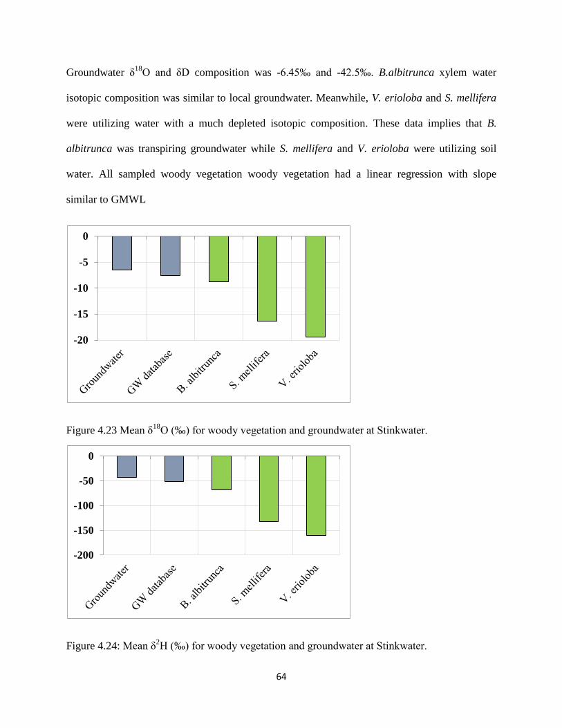
64

Groundwater δ18

O and δD composition was -6.45‰ and -42.5‰. B.albitrunca xylem water

isotopic composition was similar to local groundwater. Meanwhile, V. erioloba and S. mellifera

were utilizing water with a much depleted isotopic composition. These data implies that B.

albitrunca was transpiring groundwater while S. mellifera and V. erioloba were utilizing soil

water. All sampled woody vegetation woody vegetation had a linear regression with slope

similar to GMWL

Figure 4.23 Mean δ18

O (‰) for woody vegetation and groundwater at Stinkwater.

Figure 4.24: Mean δ2H (‰) for woody vegetation and groundwater at Stinkwater.

-20

-15

-10

-5

0

-200

-150

-100

-50

0

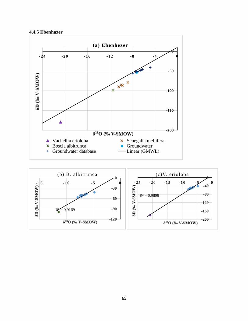
65

4.4.5 Ebenhazer

-200

-150

-100

-50

0

-2 4 -2 0 -1 6 -1 2 -8 -4 0

ΔD

(‰

V-S

MO

W)

(a) Ebenhezer

Vachellia erioloba Senegalia melliferaBoscia albitrunca GroundwaterGroundwater database Linear (GMWL)

R² = 0.9169

-120

-90

-60

-30

0

-1 5 -1 0 -5 0

AX

IS T

ITL

E

AXIS TITLE

(b) B. albi t runca

R² = 0.9898

-200

-160

-120

-80

-40

0

-2 5 -2 0 -1 5 -1 0 -5 0

AX

IS T

ITL

E

AXIS TITLE

(c)V. er ioloba

66

Figure 4.25: (a) Woody vegetation xylem water and groundwater δ2H and δ

18O compositions

with reference to GMWL. A biplot of δ18

O – δ2H showing regression relationship between

groundwater (b) B. albitrunca, (c) V.erioloba and (d) S. mellifera.

B. albitrunca and S. mellifera utilized water that was slightly depleted in δ18

O and δD in

comparison to groundwater; both are using a mixture of groundwater and soil water. Their

isotopic composition plotted close to local groundwater. Xylem water δ18

O and δD composition

for S. mellifera varied from -10.38‰ to -8.8‰ (mean: -9.72 ± 0.7‰) and -89.36‰ to -78.61‰

(mean: -84.45 ± 19.7‰). V. erioloba transpired isotopically depleted soil water, the xylem water

isotopic composition for V. erioloba was -20.78‰ and -179.0‰ for δ18

O and δD respectively.

Figure 4.0-26 Mean δ18

O (‰) for woody vegetation and groundwater at Ebenhazer.

R² = 0.9124

-100

-75

-50

-25

0

-1 5 -1 0 -5 0

AX

IS T

ITL

E

AXIS TITLE

(d) S. mel l i fera

-25

-20

-15

-10

-5

0

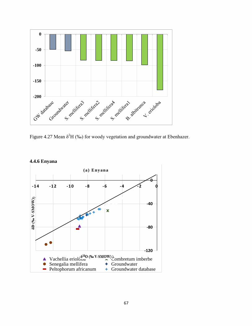
67

Figure 4.27 Mean δ2H (‰) for woody vegetation and groundwater at Ebenhazer.

4.4.6 Enyana

-200

-150

-100

-50

0

-120

-80

-40

0

-14 -12 -10 -8 -6 -4 -2 0

ΔD

(‰

V-S

MO

W)

Δ18O (‰ V-SMOW)

(a ) Enyana

Vachellia erioloba Combretum imberbeSenegalia mellifera GroundwaterPeltophorum africanum Groundwater database

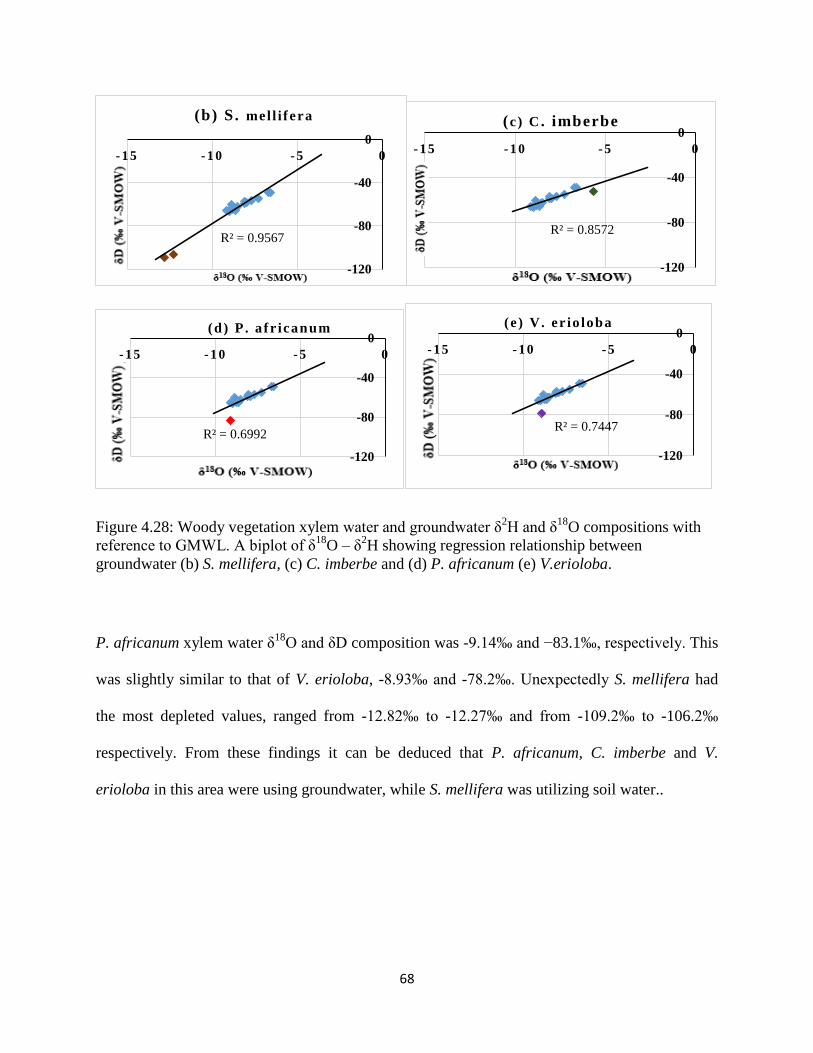
68

Figure 4.28: Woody vegetation xylem water and groundwater δ2H and δ

18O compositions with

reference to GMWL. A biplot of δ18

O – δ2H showing regression relationship between

groundwater (b) S. mellifera, (c) C. imberbe and (d) P. africanum (e) V.erioloba.

P. africanum xylem water δ18

O and δD composition was -9.14‰ and −83.1‰, respectively. This

was slightly similar to that of V. erioloba, -8.93‰ and -78.2‰. Unexpectedly S. mellifera had

the most depleted values, ranged from -12.82‰ to -12.27‰ and from -109.2‰ to -106.2‰

respectively. From these findings it can be deduced that P. africanum, C. imberbe and V.

erioloba in this area were using groundwater, while S. mellifera was utilizing soil water..

R² = 0.9567

-120

-80

-40

0

-1 5 -1 0 -5 0

AIT

LE

AXIS TITLE

(b) S. mell i f era

R² = 0.8572

-120

-80

-40

0

-1 5 -1 0 -5 0

AX

IS T

ITL

E

AXIS TITLE

(c) C . imberbe

R² = 0.6992

-120

-80

-40

0

-1 5 -1 0 -5 0

AX

IS T

ITL

E

(d) P . a fr icanum

R² = 0.7447

-120

-80

-40

0

-1 5 -1 0 -5 0

AX

IS T

ITL

E

AXIS TITLE

(e ) V. er io loba

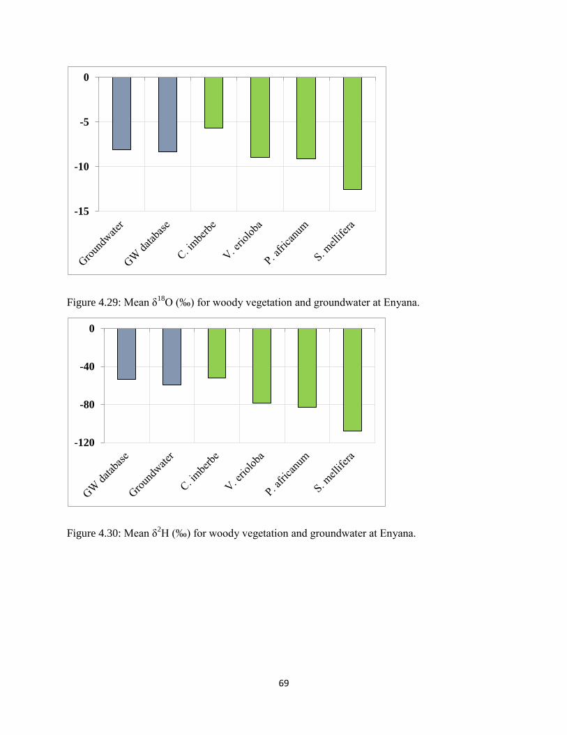
69

Figure 4.29: Mean δ18

O (‰) for woody vegetation and groundwater at Enyana.

Figure 4.30: Mean δ2H (‰) for woody vegetation and groundwater at Enyana.

-15

-10

-5

0

-120

-80

-40

0

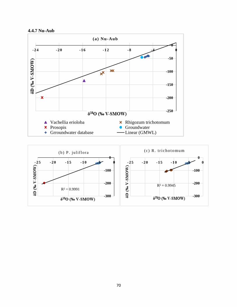
70

4.4.7 Nu-Aub

-250

-200

-150

-100

-50

0

-2 4 -2 0 -1 6 -1 2 -8 -4 0

ΔD

(‰

V-S

MO

W)

Δ18O (‰ V-SMOW)

(a) Nu-Aub

Vachellia erioloba Rhigozum trichotomumProsopis GroundwaterGrroundwater database Linear (GMWL)

R² = 0.9991

-300

-200

-100

0

-2 5 -2 0 -1 5 -1 0 -5 0

AX

IS T

ITL

E

AXIS TITLE

(b ) P . ju l i f lo ra

R² = 0.9945

-300

-200

-100

0

-2 5 -2 0 -1 5 -1 0 - 5 0

AX

IS T

ITL

E

AXIS TITLE

(c ) R . t r i chotomum

71

Figure 4.31(a) Woody vegetation xylem water and groundwater δ2H and δ

18O compositions with

reference to GMWL. A biplot of δ18

O – δ2H showing regression relationship between

groundwater (b) P. juliflora (c) R. trichotomum and (d) V. erioloba.

Isotopic compositions of waters from woody tissue of P. juliflora were more negative, followed

by V. erioloba then R. trichotomum. R. trichotomum and V. erioloba were utilizing a mixture of

soilwater and groundwater. While P. juliflora was absorbing predominantly soil water, its xylem

water δD and δ18

O values were depleted with roughly 16‰ δ18

O and 150‰ δ2H relative local

groundwater.

R² = 0.9974

-300

-200

-100

0

-2 5 -2 0 -1 5 -1 0 -5 0

AX

IS T

ITL

E

AXIS TITLE

(d)V. er ioloba

-25

-20

-15

-10

-5

0

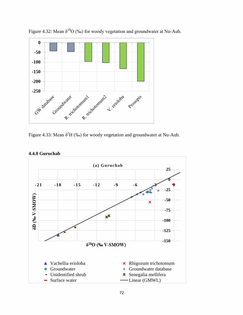
72

Figure 4.32: Mean δ18

O (‰) for woody vegetation and groundwater at Nu-Aub.

Figure 4.33: Mean δ2H (‰) for woody vegetation and groundwater at Nu-Aub.

4.4.8 Guruchab

-250

-200

-150

-100

-50

0

-150

-125

-100

-75

-50

-25

0

25

-21 -18 -15 -12 -9 -6 -3 0

AX

IS T

ITLE

AXIS TITLE

(a ) Guruchab

Vachellia erioloba Rhigozum trichotomum

Groundwater Groundwater database

Unidentified shrub Senegalia mellifera

Surface water Linear (GMWL)

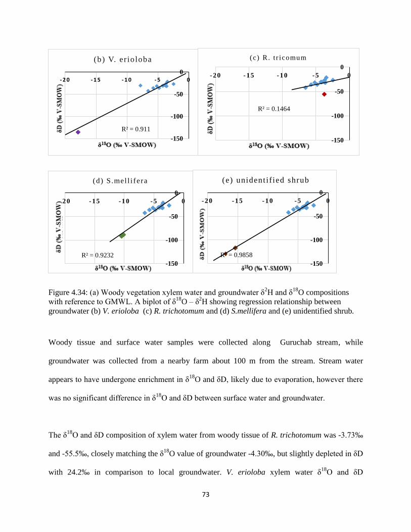
73

Figure 4.34: (a) Woody vegetation xylem water and groundwater δ2H and δ

18O compositions

with reference to GMWL. A biplot of δ18

O – δ2H showing regression relationship between

groundwater (b) V. erioloba (c) R. trichotomum and (d) S.mellifera and (e) unidentified shrub.

Woody tissue and surface water samples were collected along Guruchab stream, while

groundwater was collected from a nearby farm about 100 m from the stream. Stream water

appears to have undergone enrichment in δ18

O and δD, likely due to evaporation, however there

was no significant difference in δ18

O and δD between surface water and groundwater.

The δ18

O and δD composition of xylem water from woody tissue of R. trichotomum was -3.73‰

and -55.5‰, closely matching the δ18

O value of groundwater -4.30‰, but slightly depleted in δD

with 24.2‰ in comparison to local groundwater. V. erioloba xylem water δ18

O and δD

R² = 0.911

-150

-100

-50

0

- 2 0 - 1 5 - 1 0 - 5 0

AX

IS T

ITLE

AXIS TITLE

(b) V. er ioloba

R² = 0.1464

-150

-100

-50

0

-2 0 -1 5 -1 0 -5 0

AX

IS T

ITLE

AXIS TITLE

(c ) R . t r icomum

R² = 0.9232

-150

-100

-50

0

-2 0 -1 5 -1 0 -5 0

AX

IS T

ITLE

AXIS TITLE

(d) S .mel l i fe ra

R² = 0.9858

-150

-100

-50

0

-2 0 -1 5 -1 0 -5 0 A

XIS

TIT

LE

AXIS TITLE

(e) unident i f ied shrub

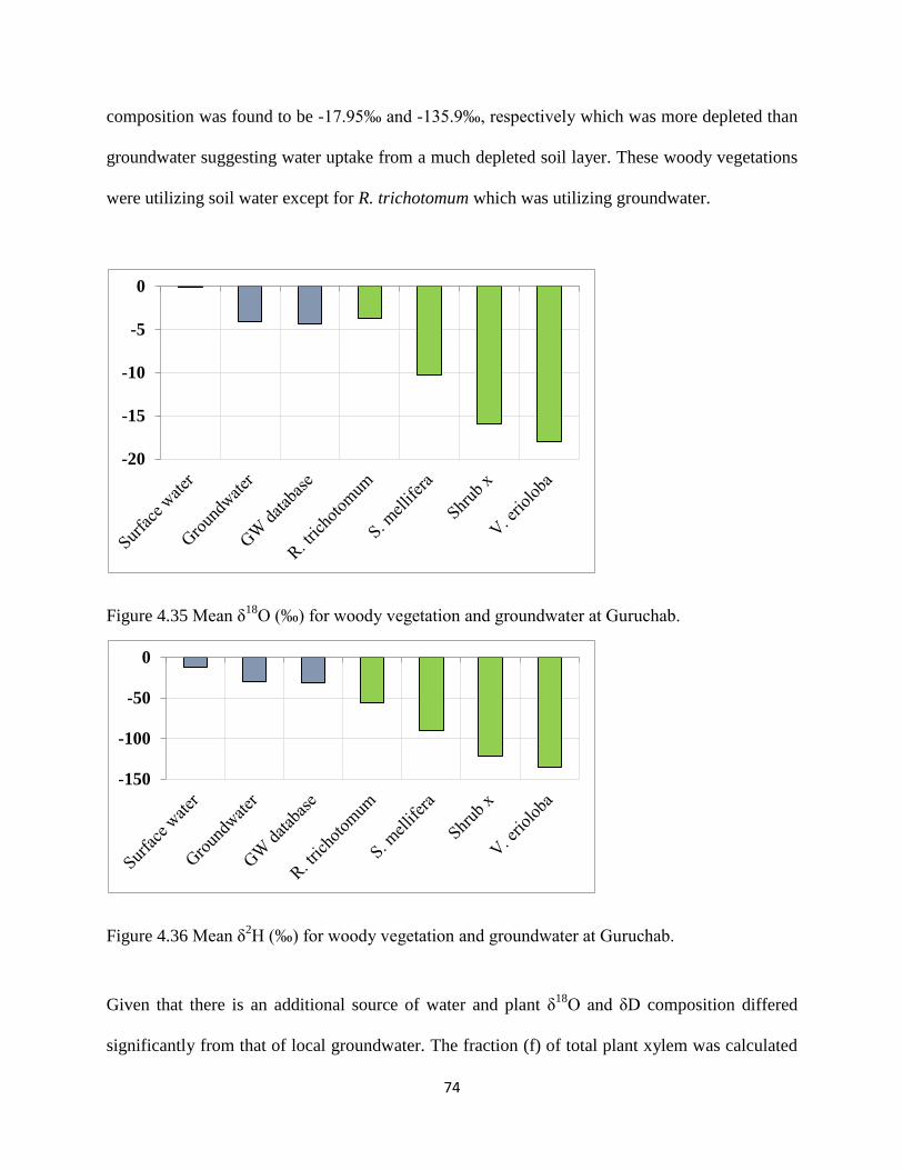
74

composition was found to be -17.95‰ and -135.9‰, respectively which was more depleted than

groundwater suggesting water uptake from a much depleted soil layer. These woody vegetations

were utilizing soil water except for R. trichotomum which was utilizing groundwater.

Figure 4.35 Mean δ18

O (‰) for woody vegetation and groundwater at Guruchab.

Figure 4.36 Mean δ2H (‰) for woody vegetation and groundwater at Guruchab.

Given that there is an additional source of water and plant δ18

O and δD composition differed

significantly from that of local groundwater. The fraction (f) of total plant xylem was calculated

-20

-15

-10

-5

0

-150

-100

-50

0

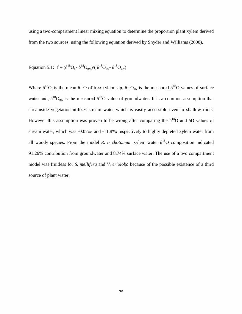
75

using a two-compartment linear mixing equation to determine the proportion plant xylem derived

from the two sources, using the following equation derived by Snyder and Williams (2000).

Equation 5.1: f = (δ18

Ot - δ18

Ogw)/( δ18

Osw- δ18

Ogw)

Where δ18

Ot is the mean δ18

O of tree xylem sap, δ18

Osw is the measured δ18

O values of surface

water and, δ18

Ogw is the measured δ18

O value of groundwater. It is a common assumption that

streamside vegetation utilizes stream water which is easily accessible even to shallow roots.

However this assumption was proven to be wrong after comparing the δ18

O and δD values of

stream water, which was -0.07‰ and -11.8‰ respectively to highly depleted xylem water from

all woody species. From the model R. trichotomum xylem water δ18

O composition indicated

91.26% contribution from groundwater and 8.74% surface water. The use of a two compartment

model was fruitless for S. mellifera and V. erioloba because of the possible existence of a third

source of plant water.

76

4.4.9 Steinhausen

Figure 4.37: (a) Woody vegetation xylem water and groundwater δ2H and δ

18O compositions

with reference to GMWL. A biplot of δ18O – δ2H showing regression relationship between

groundwater and (b) T. cericea (c) V.erioloba at Steinhousen.

T. sericea xylem water δ18

O and δD composition was 7.92‰ and 3.2‰, respectively. It plotted

on the extreme right of Global Meteoric Water Line (GMWL), indicating utilization of water

sources subject to evaporative isotopic enrichment (Williams and Ehleringer 2000). The

infiltrating rainwater underwent some enrichment of the heavier isotopes prior to recharge and/or

-80

-40

0

40

80

-8 -4 0 4 8

ΔD

(‰

V-S

MO

W)

Δ18O (‰ V-SMOW)

(a) Steinhausen

Vachellia erioloba Terminalia sericea Groundwater

Groundwater database Linear (GMWL)

R² = 0.99

-100

-50

0

-1 0 -5 0 5 1 0

AX

IS T

ITLE

AXIS TITLE

(b) T.cericea

R² = 0.7498

-100

-50

0

-1 0 -5 0

AX

IS T

ITLE

AXIS TITLE

(c) V. er ioloba

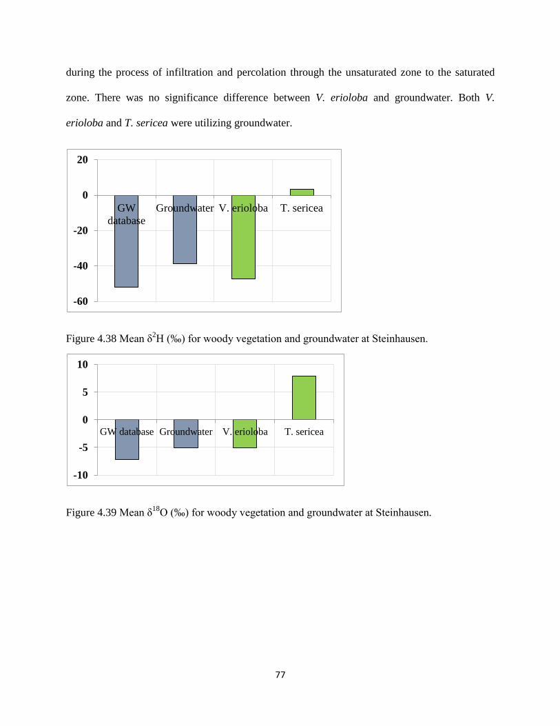
77

during the process of infiltration and percolation through the unsaturated zone to the saturated

zone. There was no significance difference between V. erioloba and groundwater. Both V.

erioloba and T. sericea were utilizing groundwater.

Figure 4.38 Mean δ2H (‰) for woody vegetation and groundwater at Steinhausen.

Figure 4.39 Mean δ18

O (‰) for woody vegetation and groundwater at Steinhausen.

-60

-40

-20

0

20

GW

database

Groundwater V. erioloba T. sericea

-10

-5

0

5

10

GW database Groundwater V. erioloba T. sericea

78

4.4.10 Warmbad

Figure 4.40: (a) Woody vegetation xylem water and groundwater δ2H and δ

18O compositions

with reference to GMWL at Warmbad.

V. erioloba was transpiring water with similar δ18

O as groundwater, but depleted with 20‰ in

δ2H. While R. trichotomum was transpiring groundwater with the same δ

18O as sampled

groundwater, but somehow enriched in δ2H. The similar behavior was observed in Guruchas

where R. trichotomum was exposed to different water sources (stream water, soil water and

groundwater), but chose to utilize only groundwater.

-60

-40

-20

0

-8 -6 -4 -2 0

ΔD

(‰

V-S

MO

W)

Δ18O (‰ V-SMOW)

Warmbad

Vachellia erioloba Rhigozum trichotomumGroundwater database GroundwaterLinear (GMWL)

79

Figure 4.41: Mean δ18O (‰) for woody vegetation and groundwater at Warmbad.

Figure 4.42: Mean δ2H (‰) for woody vegetation and groundwater at Warmbad.

-8

-6

-4

-2

0

-60

-40

-20

0

80

4.4.11 Windhoek

-200

-150

-100

-50

0

-21 -18 -15 -12 -9 -6 -3 0

ΔD

(‰

V-S

MO

W)

Δ18O (‰ V-SMOW)

(a)Windhoek

Boscia albitrunca 1 Boscia albitrunca 2 Senegalia mellifera 1

Senegalia mellifera 2 Senegalia mellifera 3 Senegalia mellifera 4

Senegalia mellifera 5 Senegalia mellifera 6 Vachellia erioloba 1

Vachellia erioloba 2 Acacia hebeclada 1 Acacia hebeclada 2

Groundwater Groundwater database Linear (GMWL)

R² = 0.8225

-200

-150

-100

-50

0

- 3 0 -2 0 -1 0 0

AX

IS T

ITL

E

AXIS TITLE

(b) B. albi t runca

R² = 0.944

-200

-150

-100

-50

0

-3 0 -2 0 -1 0 0

AX

IS T

ITL

E

AXIS TITLE

(c) S . mel l i fera

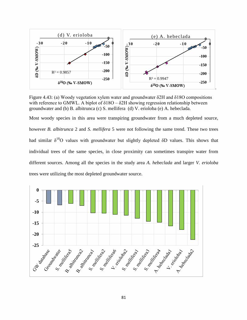
81

.

Figure 4.43: (a) Woody vegetation xylem water and groundwater δ2H and δ18O compositions

with reference to GMWL. A biplot of δ18O – δ2H showing regression relationship between

groundwater and (b) B. albitrunca (c) S. mellifera (d) V. erioloba (e) A. hebeclada.

Most woody species in this area were transpiring groundwater from a much depleted source,

however B. albitrunca 2 and S. mellifera 5 were not following the same trend. These two trees

had similar δ18

O values with groundwater but slightly depleted δD values. This shows that

individual trees of the same species, in close proximity can sometimes transpire water from

different sources. Among all the species in the study area A. hebeclada and larger V. erioloba

trees were utilizing the most depleted groundwater source.

R² = 0.9857

-250

-200

-150

-100

-50

0

-3 0 -2 0 -1 0 0

AX

IS T

ITL

E

AXIS TITLE

(d) V. er ioloba

R² = 0.9947 -250

-200

-150

-100

-50

0

-3 0 -2 0 -1 0 0

AX

IS T

ITL

E

AXIS TITLE

(e) A. hebeclada

-25

-20

-15

-10

-5

0

82

Figure 4. 44: Mean δ18O (‰) for woody vegetation and groundwater at Windhoek.

Figure 4.45: Mean δ2H (‰) for woody vegetation and groundwater at Windhoek.

-200

-150

-100

-50

0

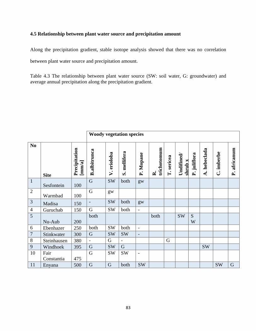
83

4.5 Relationship between plant water source and precipitation amount

Along the precipitation gradient, stable isotope analysis showed that there was no correlation

between plant water source and precipitation amount.

Table 4.3 The relationship between plant water source (SW: soil water, G: groundwater) and

average annual precipitation along the precipitation gradient.

Woody vegetation species

No

Site Pre

cip

itati

on

[mm

/a]

B.a

lbit

run

ca

V. er

iolo

ba

S. m

elli

fera

P. M

op

an

e

R.

tric

hoto

mu

m

T. se

rice

a

Un

dif

ined

/

shru

b x

P. ju

lifl

ora

A. h

ebec

lad

a

C. im

ber

be

P. afr

ican

um

1 Sesfontein 100

G SW both gw

2 Warmbad 100

G gw

3 Madisa 150 - SW both gw

4 Guruchab 150 G SW both -

5

Nu-Aub 200

both both SW S

W

6 Ebenhazer 250 both SW both -

7 Stinkwater 300 G SW SW -

8 Steinhausen 380 - G - G

9 Windhoek 395 G SW G SW

10 Fair

Constantia 475

G SW SW -

11 Enyana 500 G G both SW SW G

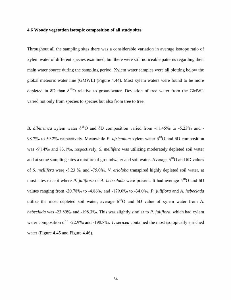
84

4.6 Woody vegetation isotopic composition of all study sites

Throughout all the sampling sites there was a considerable variation in average isotope ratio of

xylem water of different species examined, but there were still noticeable patterns regarding their

main water source during the sampling period. Xylem water samples were all plotting below the

global meteoric water line (GMWL) (Figure 4.44). Most xylem waters were found to be more

depleted in δD than δ18

O relative to groundwater. Deviation of tree water from the GMWL

varied not only from species to species but also from tree to tree.

B. albitrunca xylem water δ18

O and δD composition varied from -11.45‰ to -5.23‰ and -

98.7‰ to 59.2‰ respectively. Meanwhile P. africanum xylem water δ18

O and δD composition

was -9.14‰ and 83.1‰, respectively. S. mellifera was utilizing moderately depleted soil water

and at some sampling sites a mixture of groundwater and soil water. Average δ18

O and δD values

of S. mellifera were -8.23 ‰ and -75.0‰. V. erioloba transpired highly depleted soil water, at

most sites except where P. juliflora or A. hebeclada were present. It had average δ18

O and δD

values ranging from -20.78‰ to -4.86‰ and -179.0‰ to -34.0‰. P. juliflora and A. hebeclada

utilize the most depleted soil water, average δ18

O and δD value of xylem water from A.

hebeclada was -23.89‰ and -198.3‰. This was slightly similar to P. juliflora, which had xylem

water composition of ` -22.9‰ and -198.8‰. T. sericea contained the most isotopically enriched

water (Figure 4.45 and Figure 4.46).

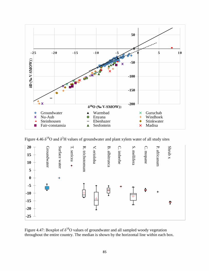
85

Figure 4.46 δ18

O and δ2H values of groundwater and plant xylem water of all study sites

Figure 4.47: Boxplot of δ18

O values of groundwater and all sampled woody vegetation

throughout the entire country. The median is shown by the horizontal line within each box.

-200

-150

-100

-50

0

50

-2 5 -2 0 -1 5 - 1 0 -5 0 5 1 0

ΔD

(‰

V-S

MO

W)

Δ18O (‰ V-SMOW)

Groundwater Warmbad GuruchabNu-Aub Enyana WindhoekSteinhousen Ebenhazer StinkwaterFair-constansia Sesfontein Madisa

Gro

undw

ater

Surface w

ater

T. sericea

R. trich

oto

mum

V. erio

loba

B. alb

itrunca

C. im

berb

e

S. m

ellifera

C. m

opan

e

P. africanum

Shru

b x

-25

-20

-15

-10

-5

0

5

10

15

20

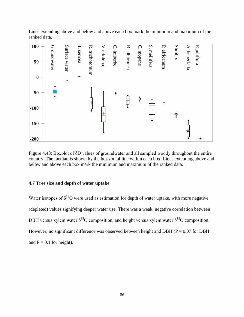
86

Lines extending above and below and above each box mark the minimum and maximum of the

ranked data.

Figure 4.48: Boxplot of δD values of groundwater and all sampled woody throughout the entire

country. The median is shown by the horizontal line within each box. Lines extending above and

below and above each box mark the minimum and maximum of the ranked data.

4.7 Tree size and depth of water uptake

Water isotopes of δ18

O were used as estimation for depth of water uptake, with more negative

(depleted) values signifying deeper water use. There was a weak, negative correlation between

DBH versus xylem water δ18

O composition, and height versus xylem water δ18

O composition.

However, no significant difference was observed between height and DBH (P = 0.07 for DBH

and P = 0.1 for height).

Gro

undw

ater

Surface w

ater

T. sericea

R. trich

oto

mum

V. erio

loba

C. im

berb

e

B. alb

itrunca

C. m

opan

e

S. m

ellifera

P. africanum

Sh

rub x

A. h

ebeclad

a

P. juliflo

ra

-200

-150

-100

-50

0

50

100

87

Figure 4.49: Relationship between δ18

O of xylem water and diameter at 1.4m of tree/shrub.

Figure 4.50: The relationship between δ18

O of xylem water and tree/shrub height.

R² = 0.09

0

20

40

60

80

100

-30 -20 -10 0 10

DB

H(c

m)

y = -0.35x + 4.68

R² = 0.08

0

10

20

30

40

-30 -20 -10 0 10

Hei

gh

t (m

)

δ18O (‰ V-SMOW)

88

CHAPTER 5

5. Interpretation and Discussion

5.1 Groundwater isotopic variation

Different recharge components can be identified through the stable isotope composition of

groundwater, because evaporation during groundwater recharge leads to an increase in the

proportion of the heavy isotopes D and 18

O. Rates of evaporation are determined by several

factors, including temperature, solar radiation, humidity, wind speed and atmospheric pressure

(Mendelsohn et al., 2002). According to Mendelsohn et al. (2002) the degree of water deficit- the

difference between average annual rainfall and average rate of evaporation is highest in the

south-east and gradually decrease towards the north east as a result of higher rainfall and less

evaporation. Most groundwater samples plotted above the GMWL, which reflects the significant

impact of evaporation.

The isotopic composition is depleted in the groundwater from Kalahari porous aquifers (Enyana

and Fair-Constantia), while enriched in the fractured rock aquifers (Stienhausen, Madisa and

Windhoek) these isotopically heavier groundwater samples may be attributed to the impact of

evaporation before or during infiltration. Guruchas had the most enriched isotope values which

correspond to the highest average annual evaporation rates of >3800 mm/year. Windhoek,

Stinkwater and Ebenhazer had groundwater samples moderately depleted and moderate average

annual evaporation rates 2100-2240 mm/year. Enyana and Fair-Constantia had the most depleted

values and the least average annual evaporation rates 1820- 1960 mm/year and 2240-2380

mm/year respectively.

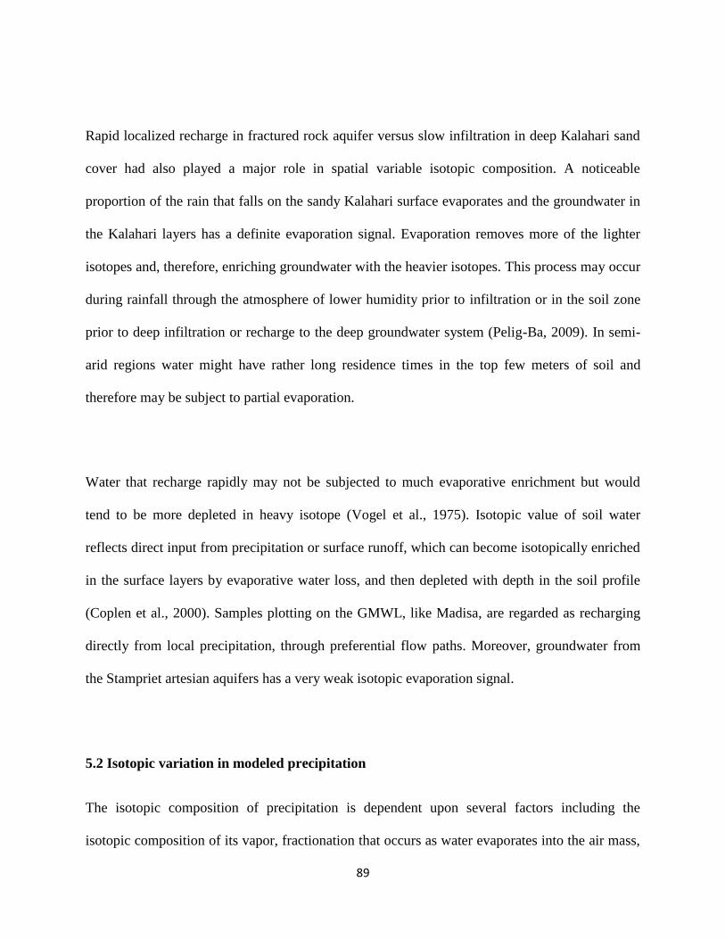
89

Rapid localized recharge in fractured rock aquifer versus slow infiltration in deep Kalahari sand

cover had also played a major role in spatial variable isotopic composition. A noticeable

proportion of the rain that falls on the sandy Kalahari surface evaporates and the groundwater in

the Kalahari layers has a definite evaporation signal. Evaporation removes more of the lighter

isotopes and, therefore, enriching groundwater with the heavier isotopes. This process may occur

during rainfall through the atmosphere of lower humidity prior to infiltration or in the soil zone

prior to deep infiltration or recharge to the deep groundwater system (Pelig-Ba, 2009). In semi-

arid regions water might have rather long residence times in the top few meters of soil and

therefore may be subject to partial evaporation.

Water that recharge rapidly may not be subjected to much evaporative enrichment but would

tend to be more depleted in heavy isotope (Vogel et al., 1975). Isotopic value of soil water

reflects direct input from precipitation or surface runoff, which can become isotopically enriched

in the surface layers by evaporative water loss, and then depleted with depth in the soil profile

(Coplen et al., 2000). Samples plotting on the GMWL, like Madisa, are regarded as recharging

directly from local precipitation, through preferential flow paths. Moreover, groundwater from

the Stampriet artesian aquifers has a very weak isotopic evaporation signal.

5.2 Isotopic variation in modeled precipitation

The isotopic composition of precipitation is dependent upon several factors including the

isotopic composition of its vapor, fractionation that occurs as water evaporates into the air mass,

90

precipitation formation processes, and air mass trajectory. Most of these factors are

predominantly due to fractionation (McGuire and McDonnell, 2006). Four major causes of

variation in precipitation stable isotope ratios are: altitude, latitude, distance from the oceanic

vapour source area and amount of precipitation (Dansgaard, 1964). These factors are discussed

below.

5.2.1 Continental effect

Continental effect is the observation that meteoric water is more depleted further from the source

of the water vapor. Rainout reduces the heavy isotopic composition of an air mass as it travels

inland. Isotopic composition of the condensing precipitation is more enriched than that of the

remaining vapor due to due to isotopic fractionation during condensation. The 2H and

18O

content decrease in precipitation with increasing distance from the coast due to rainout (Coplen

et al., 2000; Kendall and McDonnell, 1998).

The observed continental effect was 3.1‰ depletion in δ18

O per km across Namibia. Highest

δ18

O values were found in Guruchas (-6.3‰) and Warmbad (-5.1‰) due to close proximity with

their water vapor source the Atlantic Ocean. Lowest values were found in Fair Constantia and

Enyana where the rainout process has evolved to low residual vapor fractions since these sites

are distant from their source, the Indian Ocean.

The average δ18

O isotopic gradients hwas greater than what have been measured in the Amazon

basin and Europe, <1 ‰/1000 km and 2‰/1000 km respectively (Rozanski et al., 1993). As

91

well as the Pacific Northwest, USA 12 ‰/1000 km (Welker, 2000) and Sierra Nevada, USA

50‰/1000 km (Ingraham and Taylor, 1991).

5.2.2 Latitude effect

Latitude effect is characterized by decrease in δ18

O and δ2H values in precipitation with

increasing latitude. These isotopic variations are caused by cooler temperatures that air masses

encounter as they proceed from equatorial regions. On a whole-country scale, the precipitation

δ18

O value depletes approximately 0.37‰ for every one degree southward in latitude. The

latitude effect was quite noticeable in most samples for instance groundwater δ18

O composition

at Enyana at latitude of -17.6° , was -8.1 ‰, while Warmbad, latitude -28.4°, groundwater δ18

O

value were -5.69‰. The latitude effect results from increased evolution of the air mass due to

increased isotopic fractionation at the cooler temperature of condensation in a manner similar to

that responsible for the elevation effect (Kendall and McDonnell, 1998).

The observed latitude effect is lower than the effect observed for coastal and continental stations

in Europe and the USA, i.e. 0.6‰/degree of latitude (Mook, 2001) which might be due to an

overprint by other effects and/or influenced by higher temperatures in the study area.

5.2.3 Altitude effect

Elevation effect is the observation that the stable isotopic compositions of meteoric water are

more depleted at higher elevation. The lowering of temperature with increasing elevation leads to

enhanced condensation and therefore to a progressive depletion in heavy isotopes of

precipitation. In this study isotopic data on precipitation did not show a clear trend with altitude.

92

The altitude effect was poorly correlated due to different precipitation sources and nature of low

elevation gradient. The δ18

O values of precipitation decreases at 0.13‰ per 100 m rise in

altitude. Heavy isotope content of precipitation does not decrease always in the same manner

with the altitude (Gonfiantini et al., 2001). This was observed in the results, for example Fair

Constantia, elevation 1500 m above sea level had the most depleted δ18

O values -10.7‰ than

Windhoek (-7.1‰) which has highest elevation approximately 1700 m above sea level.

The observed altitude effects are consistent with altitude effects found on continental Africa e.g.

for Mount Cameroon (-0.156‰) (Gonfiantini et al., 2001) but smaller than for Mount Kenya (-

0.27‰) (Tongiorgi, 1970). However, the observed altitude effect in this study is consistent with

the general magnitude of the altitude effect, i.e. between -0.1 up to -0.6‰/100 m worldwide

(Vogel et al., 1975).

5.2.4 Amount effect

Amount effect is described as a negative correlation between δ18

O and the amount of monthly

precipitation (Dansgaard, 1964). It is a consequence of a Raleigh condensation and rainout

process of atmospheric vapor. Enyana and Fair Constantia had the highest average annual

rainfall corresponding to the most depleted δ18

O values. Sites with summer rainfall had depleted

δ18

O values than winter rainfall this is because they are originated from Intertropical

Convergence Zone (ITCZ) and rain at these sites is a later stage product. Precipitation isotopic

values decrease with increasing monthly or annual mean precipitation, thus higher rainfall

amount tend to have isotopic composition that are more depleted in 2H and

18O than more

frequent lighter precipitation events (Coplen et al., 2000).

93

5.3 Water uptake by plants

In arid and semi-arid-regions water used by vegetation may only be available from the very top

soil layer (0-50cm), directly derived from recent rainfall or from the groundwater (Brunel et al.,

1991). In this study the δD and δ18

O data indicated that B. albitrunca, C. mopane and C.

imberbe, R. trichotomum and T. sericea were mainly using groundwater.

It was hypothesized that the encroacher species R. trichotomum and S. mellifera were utilizing

soil water and this gives them an advantage over non-encroachers. However, isotopic ratios of

xylem sap indicated that R. trichomum predominantly utilized groundwater while S. mellifera

utilized a mixture of groundwater and available soil water that was more negative than

groundwater. The water uptake pattern of these species is highly attributed to their rooting

system. S. mellifera has relatively shallow, but extensive rooting system (maximum rooting

depth ±4.5m) (Canadell et al., 1996), while R. trichotomum have a well-developed root system

up to three times wider than the height of the plant (Union, 2010).

Dawson and Ehleringer (1998) reported that encroacher species were able to access both shallow

and deeper water sources whereas the original pasture vegetation only accessed deep water.

These encroaching plants affect aquifers by directly extracting groundwater from saturated strata

and by reducing the proportion of rainfall that is recharged. Much of the groundwater is situated

at depths where it is unlikely for shallow-rooted woody species such as S. mellifera to reach. It is

assumed that these plants were utilizing water drawn by deep rooted species such as B.

albitrunca and V. erioloba from the groundwater aquifer, transported upward in the root system

into a drier upper soil layer which is at a lower water potential, a phenomenon known as

hydraulic lift (Horton and Hart, 1998). The shallow root system of these vegetation and hydraulic

94

lifting was the reason why it was able to access stored soil water instead of groundwater

throughout the dry season.

Hydraulically lifted water source allows small trees to continue transpiration when they normally

would not. The physical basis behind hydraulic lift is best explained in terms of various

components of water potential in the root zone. In areas where transpiration and evaporation are

removing soil moisture from shallow surface soils, the total water potentials will decrease or

become more negative. Water from deeper soil layers with less negative water potentials will

then move upward towards the surface to replenish this lost water (Landmeyer, 2011).

T. sericea, a shallow rooted tree that prefers growing on very sandy soils had the most

isotopically enriched xylem water. One explanation for the more enriched xylem water would be

that the source water was a large shallow reservoir where accelerated evaporative isotopic

enrichment took place. Isotopic ratios for groundwater in “closed basins” are typically more

enriched than the meteoric water that feeds them. Meanwhile, C. mopane was transpiring a

mixture of groundwater and soil water. C. mopane has an extensive root system with large

proportion of the roots concentrated to shallow depth where they actively compete with shallow

rooted herbaceous plants by intercepting most of the available soil water (Christian, 2010).

The δ18

O and δD data further showed that plants with deep roots such as B .albitrunca, V.

erioloba and P. juliflora accessed isotopically depleted soil water and groundwater. Apart from

deep roots, these trees also have extensive lateral root development that enables them to take

advantage of sparse precipitation. Studies by February and Schachtschneider and February

95

(2013) have shown that V. erioloba and P. juliflora compete for the same water and this have

negative impact on available water, species diversity and ecosystem function through the decline

in viability of V. erioloba.

Observed δ18

O and δD compositions of P. africanum, T. sericea, S. mellifera, A. hebeclada, R.

trichotomum and P. juliflora showed evidence of transpiring water from an isotopically separate

pool from groundwater or stream water. According to Evaristo et al. (2015) this phenomenon is

known as “Eco-hydrological Compartmentalization” whereby the isotopic composition of water

that supply plant transpiration differs from that of waters that supply groundwater and

streamflow. This is because, soil water that supplies plant transpiration is isolated from the water

that recharges groundwater and replenishes streamflow.

The large amount of variation observed in woody vegetation δ2H and δ

18O compositions

suggests that trees were using water from a reliable water source, but it may indicate that trees

are using old stored soil water from past percolation rainfall or irrigation events. However, more

commonly it is caused by phase changes such as condensation events when water vapor in the

soil airspace/ matrix reaches its dew-point as the soil becomes cooler with depth (Kendall and

McDonnell, 1998). These erratic values could also be due to cryogen vacuum distillation method

used to extract xylem water.

96

CHAPTER 6

6. Conclusions

The study’s main objective was to identify plant water source of woody vegetation in Namibian

Savanna aquifers along a precipitation gradient. This principal assumption underlying this study

is that water is not isotopically fractionated when taken up by the plant (Dawson and Ehleringer

1998) and plant tissues are expected to carry the same isotopic composition as the source water.

The stable isotope studies here have proven to be an effective method in determining plant water

source. Results have shown that deep rooted species such as V. erioloba, P. juliflora and A.

hebeclacada mostly transpired the mostly depleted soil water recharged from heavy rainfall. In

large rainfall events, precipitation can complement deep soil moisture and function as a reservoir

such that plants can consume this portion of water in the next period when plants experience

drought stress (Huang and Zhang, 2015). While shallow rooted species such as C. mopane and S.

mellifera utilized a mixture of soil water and groundwater hydraulically lifted by deep rooted

trees.

In contrast to the study’s original hypothesis that woody vegetation of the Savanna ecosystem

utilizes groundwater in dry areas and soil water in wetter areas, it has been found that woody

savanna vegetation generally rely on soil water, groundwater or both for transpiration. Plant

water source vary from specie to specie and it is not influenced by precipitation amount or tree

size. Savanna woody vegetation in Namibia uptakes groundwater and soil water in a hierarchical

manner at different depths in order to ward off competition between species. Based on these

findings, in areas where large amount of water are to be extracted for water supply, monitoring

of groundwater levels is necessary to avoid negative impact on woody vegetation especially of

97

protected species. Woody vegetation requires water for consumptive use as well as for

biophysical processes.

The water source utilization of these plants is consistent with the two layer theory developed by

Walter (1971). This theory states that woody and herbaceous plants are able to coexist in savanna

because they utilize water from different soil depths. Woody plants have a larger proportion of

roots in deeper layers taking considerably more soil water. These plants have evolved dimorphic

roots that absorb shallow soil water in rainy season and deep soil water in arid seasons (Yang et

al., 2010).

The observed spatial variability in δ18

O and δ2H values of xylem water in woody tissues at

different sampling sites along the precipitation gradient are attributed mainly to latitude and

amount effect in the source water, i.e. precipitation that becomes surface water, soil water or

groundwater and is later taken up by the vegetation. Groundwater samples plotted below the

GMWL and thus indicate the effects of evaporation attributed to high temperatures, low relative

humidity, and slow infiltration rates through the top soil layers. Nevertherless groundwater

samples plot approximately along the GMWL, this pattern suggest groundwater to follow the

local precipitaion input signal (Evaristo et al., 2015). Overall the tree xylem δ18

O and δD

composition showed evidence of a stronger evaporative signal compared to groundwater.

Plant xylem water showed evidence of originating from an isotopically separate pool from

groundwater and it may indicate that trees are using deep soil water from an earlier season or

year. The observed in δ18

O and δD compositions in xylem water of all sampled woody

98

vegetation suggests that they were using water from a reliable source, which points to

groundwater or deep soil water rather than shallow soil water or surface water as the main source

of water supporting transpiration.

99

REFERENCES

Alias, D., Milton, S., Herrmann, E., Seymour, C., 2003. A collation and overview of research

information on Boscia albitrunca (shepherd’s tree) and identification of relevant

research gaps to inform protection of the species. Department of Water Affairs and

Forestry.

Brunel, J. P., Walker, G. R., Walker, C. D., Dighton, J. C., Kennett-Smith, A., 1991. Using stable

isotopes of water to trace plant water uptake. Stable isotopes in plant nutrition, soil

fertility and environmental studies, 543-51.

Brunel, J. P., Walker, G. R., Kennett-Smith, A. K., 1995. Field validation of isotopic procedures

for determining sources of water used by plants in a semi-arid environment. Journal of

Hydrology, 167(1-4), 351-368.

Canadell, J., Jackson, R. B., Ehleringer, J. B., Mooney, H. A., Sala, O. E., Schulze, E. D., 1996.

Maximum rooting depth of vegetation types at the global scale. Oecologia. 108(4), 583-

595.

Christelis, G., Struckmeier, W., 2011. Groundwater in Namibia: An explanation to the

hydrogeological map, Ministry of Agriculture, Water and Rural Development,

Windhoek, Namibia, p. 132.

Christian, C., 2010. The Effect of Bush Encroachment on Groundwater Resources in Namibia: A

Desk Top Study.

Clark, I., Fritz, P., 1997. Environmental isotopes in Hydrology. Lewis Publishers, New York.

100

Coplen, T. B., Herczeg, A. L., Barnes, C., 2000. Isotope engineering - using stable isotopes of

the water molecule to solve practical problems. In Environmental tracers in subsurface

hydrology (pp. 79-110). Springer US.

Craig, H., 1961. Isotopic variations in meteoric waters. Science. 133(3465), 1702-1703.

Dawson, T. E., Ehleringer, J. R., 1998. Plants, isotopes and water use: a catchment-scale

perspective. Isotope tracers in catchment hydrology, 165-202.

Dawson, T. E., Ehleringer, J. R. 1991. Streamside trees that do not use stream water. Nature.

350, 335-337.

Dawson, T. E., Mambelli, S., Plamboeck, A. H., Templer, P. H., Tu, K. P., 2002. Stable isotopes

in plant ecology. Annual review of ecology and systematics, 507-559.

De Klerk, J. N., 2004. Bush Encroachment in Namibia: Report on Phase 1 of the Bush

Encroachment Research, Monitoring, and Management Project. Ministry of

Environment and Tourism, Directorate of Environmental Affairs.

Dansgaard, W., 1964. Stable isotopes in precipitation. Tellus, 16(4), 436-468.

Ehleringer, J. R., Dawson, T. E., 1992. Water uptake by plants: perspectives from stable isotope

composition. Plant, Cell & Environment. 15(9), 1073-1082.

Eamus, D., 2006. Ecohydrology: vegetation function, water and resource management. Csiro

Publishing.

Eamus, D., Chen, X., Kelley, G., Hutley, L. B., 2002. Root biomass and root fractal analyses of

an open Eucalyptus forest in a savanna of north Australia. Australian Journal of

Botany. 50(1), 31-41.

101

Evaristo, J., Jasechko, S., McDonnell, J. J., 2015. Global separation of plant transpiration from

groundwater and streamflow. Nature. 525(7567), 91-94.

Fuggle, R. F., Rabie, M. A., 1992. Environmental management in South Africa. Juta and

Company.

Gaines, K. P., Stanley, J. W., Meinzer, F. C., McCulloh, K. A., Woodruff, D. R., Chen, W.,

Adams, T.S., Lin, H.,Eissenstat, D. M., 2016. Reliance on shallow soil water in a

mixed-hardwood forest in central Pennsylvania. Tree physiology. 36(4), 444-458.

Giess, W., 1971. A preliminary vegetation map of South West Africa. Dinteria 4: 5-114.

Gonfiantini, R., Roche, M. A., Olivry, J. C., Fontes, J. C., Zuppi, G. M., 2001. The altitude effect

on the isotopic composition of tropical rains. Chemical Geology. 181(1), 147-167.

Herczeg, A. L., Leaney, F. W., 2011. Review: environmental tracers in arid-zone

hydrology. Hydrogeology Journal. 19(1), 17-29.

Horton, J. L. Hart, S. C., 1998. Hydraulic lift: a potentially important ecosystem process. Trends

in Ecology & Evolution. 13(6), 232-235.

Ingraham, N.L., 1998. Isotopic variations in precipitation. In: C. Kendall and J. McDonnell

(eds.), Isotope Tracers in Catchment Hydrology. Elsevier, Amsterdam, pp. 98-118.

Ingraham, N. L., Taylor, B. E., 1991. Light stable isotope systematics of large‐ scale hydrologic

regimes in California and Nevada. Water Resources Research. 27(1), 77-90.

Jonsson, E.C., Leng, J.M., Rosqvist, C.G., Seibert, J., Arrowsmith, C., 2009. Stable oxygen and

hydrogen isotopes in sub-Arctic lake waters from northern Sweden. Journal of

Hydrology. 376, 143–151.

102

Kendall, C., McDonnell, J. J., 1998. Isotope tracers in catchment hydrology. Elsevier.

Kinzelbach, W., Aeschbach, W., Alberich, C., Goni, I. B., Beyerle, U., Brunner, P., Chiang W.-

H., Rueedi, J., Zoellmann, K., 2002. A survey of methods for groundwater recharge in

arid and semi-arid regions. Early warning and assessment Report series,

UNEP/DEWA/RS, 2(2).

Kresic, N., 2008. Groundwater resources: Sustainability, management, and restoration. McGraw

Hill Professional, New York.

Landmeyer, J. E., 2011. Introduction to phytoremediation of contaminated groundwater:

Historical foundation, hydrologic control, and contaminant remediation. Springer

Science & Business Media

Lubis, E. M., Harahap, Y. I., Hidayat, T. C., Pangaribuan, Y., Sutarta, E. S., Rahman, Z. A.,

2004. Stable Oxygen and Deuterium Isotope Techniques to Identify Plant Water

Sources. Journal of Water Resource and Protection. 6, 1501-1508.

Mannheimer, C. A., Curtis, B. A., (eds) (2009) Le Roux and Müller’s Field Guide to the Trees

and Shrubs of Namibia. Macmillan Education Namibia.

McGuire, K.J., McDonnell, J. J., 2006. Stable isotope tracers in watershed hydrology. In: K.

Lajtha and R. Michener (Eds), Stable Isotopes in Ecology and Environmental Science.

Mendelsohn, J., Jarvis, A., Roberts, C., Robertson, T., 2002. Atlas of Namibia, Published for the

Ministry of Environment and Tourism by David Philip.

Miller, R.M., 2008. The Geology of Namibia. In: Neoproterozoic to Lower Paleozoic (Vol. 2).

Geological Survey of Namibia, Windhoek, Namibia.

103

Midgeley, D. C., Pitman, W. V., Middleton, B. J., 1994. Surface Water Resources of South

Africa 1990. WRC Report Nos. 298/1/94 to 298/6.2/94. Water Research Commission,

Pretoria, South Africa.

Mook, W.G., 2001. Environmental isotopes in the Hydrological Cycle. UNESCO/IAEA Series.

Msangi, J. P., 2014. Food Security among Small-Scale Agricultural Producers in Southern

Africa. Springer.

Nimmo, J. R., Healy, R. W., Stonestrom, D. A., 2005. Aquifer recharge. Encyclopedia of

Hydrological Sciences.

Obakeng, O. T., 2007. Soil moisture dynamics and evapotranspiration at the fringe of the

Botswana Kalahari, with emphasis on deep rooting vegetation, PhD Dissertation,

Dissertation No. 141, ITC, Enschede

Oldeland, J., Dorigo, W., Wesuls, D., Jürgens, N., 2010. Mapping bush encroaching species by

seasonal differences in hyperspectral imagery. Remote Sensing. 2(6), 1416-1438.

Orwa C, A Mutua, Kindt R, Jamnadass R, S Anthony., 2009. Agroforestree Database:a tree

referenceandselectionguideversion4.0http://www.worldagroforestry.org/treedb/AFTPD

FS/Peltophorum_africanum.PDF.

Picarro L2120-i δD/δ18

O isotopic water analyzer: http:

//www.picarro.com/sites/default/files/L2120-i%20Datasheet.pdf (accessed 31 August

2016), 2012.

Pelig-Ba, K. B., 2009. Analysis of stable isotope contents of surface and underground water in

two main geological formations in the Northern region of Ghana. West African Journal

of Applied Ecology. 15(1).

104

Roberts, J., 2000. The influence of physical and physiological characteristics of vegetation on

their hydrological response. Hydrological Processes. 14(16‐ 17), 2885-2901.

Rossatto, D. R., Silva, L. C. R., Sternberg, L. S. L.,Franco, A. C., 2014. Do woody and

herbaceous species compete for soil water across topographic gradients? Evidence for

niche partitioning in a Neotropical savanna. South African Journal of Botany. 91, 14-

18.

Rozanski, K., Araguás‐ Araguás, L., Gonfiantini, R., 1993. Isotopic patterns in modern global

precipitation. Climate change in continental isotopic records, 1-36.

Schachtschneider, K., February, E. C., 2013. Impact of Prosopis invasion on a keystone tree

species in the Kalahari Desert. Plant Ecology. 214(4), 597-605.

Snyder, K. A., Williams, D. G., 2000. Water sources used by riparian trees varies among stream

types on the San Pedro River, Arizona. Agricultural and Forest Meteorology. 105(1),

227-240.

Sophocleous, M., 2004. Groundwater recharge. Luis Silveira, E.J. Usunoff (Eds.), Groundwater,

in Encyclopedia of Life Support Systems (EOLSS), vol. I, Developed under the

auspices of the UNESCO, EOLSS, Publishers, Oxford, UK (2004), p. 41.

Sweet, J., Burke, A., 2000. Country Pasture/Forage Resource Profiles. Namibia. FAO. Access:

http://www. fao. org/ag/AGP/AGPC/doc/Counprof/Namibia/namibia. htm, 2.

Tongiorgi, E., 1970. Isotope Hydrology 1970B. IAEA, Vienna, pp. 43–57.

Turewicz, V., 2013. Stable isotopes of waters in Namibia (Unpublished BSc Thesis). University

of Cologne, Germany.

105

Union, N. N. A., 2010. The Effect of Bush Encroachment on Groundwater Resources in

Namibia: a Desktop Study. Final Report.

Vogel, J.C., Lerman J.C., and Mook W.G., 1975. Natural isotopes in surface and groundwater

from Argentina. Hydrological Sciences Bulletin.20, 203–220.

Walker, G., Brunel, J. P., Dighton, J., Holland, K., Leaney, F., McEwan, K., Mensforth, L.,

Thorburn, P., Walker, C., 2001. The use of stable isotopes of water for determining

sources of water for plant transpiration. In Stable Isotope Techniques in the Study of

Biological Processes and Functioning of Ecosystems (pp. 57-89). Springer Netherlands.

Walter, H., 1971. Natural savannahs as a transition to the arid zone. Ecology of tropical and

subtropical vegetation. Oliver and Boyd, Edinburgh, 238-265.

Ward, D., 2005. Do we understand the causes of bush encroachment in African

savannas?. African Journal of Range and Forage Science. 22(2), 101-105.

Welker, J. M., 2000. Isotopic (δ18

O) characteristics of weekly precipitation collected across the

USA: an initial analysis with application to water source studies. Hydrological

Processes. 14(8), 1449-1464.

West, A. G., Patrickson, S. J., Ehleringer, J. R., 2006. Water extraction times for plant and soil

materials used in stable isotope analysis. Rapid Communications in Mass

Spectrometry. 20(8), 1317-1321.

Williams, D. G., Ehleringer, J. R., 2000. INTRA AND INTERSPECIFIC VARIATION FOR

SUMMER PRECIPITATION USE IN PINYON–JUNIPER

WOODLANDS. Ecological Monographs, 70(4), 517-537.

106

Yang, Q., Xiao, H., Zhao, L., Zhou, M., Li, C., Cao, S., 2010. Stable isotope techniques in plant

water sources: a review. Sciences in Cold and Arid Regions. 2(2), 0112–0122.

Yidana, S. M., 2015. The Stable Isotope Characteristics of Groundwater in the Voltaian Basin an

Evaluation of the Role of Meteoric Recharge in the Basin. Hydrogeology & Hydrologic

Engineering, 2013.

Yin, L., Zhou, Y., Huang, J., Wenninger, J., Zhang, E., Hou, G., Dong, J., 2015. Interaction

between groundwater and trees in an arid site: Potential impacts of climate variation

and groundwater abstraction on trees. Journal of Hydrology. 528, 435-448.

Zencich, S. J., Froend, R. H., Turner, J. V., Gailitis, V., 2002. Influence of groundwater depth on

the seasonal sources of water accessed by Banksia tree species on a shallow, sandy

coastal aquifer. Oecologia. 131(1), 8-19.

Zimmermann, U., Ehhalt, D., Munnich, K. O., 1967. Soil-water movement and evaporation:

changes in isotopic composition of the water. In: Knippner M (ed) Proceedings of the

symposium on isotopes in hydrology. IAEA, Vienna.

107

Appendix

Table A.1: Data used in this study: site, species, xylem water isotopic composition, diameter at

breast& height (1.4 m) and crown diameter.

Sample

ID

Site Species δ18

O

(‰)

δ2H

(‰)

DBH(cm) Height

(m)

Crown

Diameter

(m)

CK-1 Madisa C. mopane -8.81 -76.7 85 7

CK-2 Madisa V. erioloba -13.96 -114.3 69 8.5

CK-3 Madisa S. mellifera -6.72 -81.2 Multi-

stemed

2.5

CK-4 Seisfontein V. erioloba -9.41 -91.7 31.8 5.5

CK-5 Seisfontein C. mopane -6.99 -64.2 24,28.6&

38

6.5

CK-6 Seisfontein B. albitrunca -6.48 -59.2 16& 20 5.1

CK-7 Fair

Constantia

V. erioloba -14.97 -124.6 41 & 35 7

CK-8 Fair

Constantia

B. albitrunca -5.23 -59.3 30.8 6.5

CK-9 Fair

Constantia

S. mellifera -15.69 -136.6 Multi-

stemed

2.5

CK-10 Stinkwater V. erioloba -19.41 -160.1 29 8

CK-11 Stinkwater S. mellifera -15.65 -128.1 Multi-

stemed

3

S. mellifera -17.46 -140.1

S. mellifera -16.01 -129.1

CK-12 Stinkwater B. albitrunca -8.80 -67.9 42.7 7.5

CK-13 Ebenhazer V. erioloba -20.78 -179.0 22.6 4.5

CK-14 Ebenhazer S. mellifera -9.73 -85.7 11 4

Ebenhazer S. mellifera -10.38 -89.4

S. mellifera -8.80 -78.6

S. mellifera -9.97 -84.8

CK-15 Ebenhazer B. albitrunca -11.45 -98.7 30 5

CK-16 Steinhausen V. erioloba -5.05 -47.2 16.5 4.5

CK-17 Steinhausen T. sericea 7.92 3.2 24.8 7

CK-18 Windhoek B. albitrunca -10.38 -93.1 7, 7.6

&10.8

10 6 by 6

CK-19 Windhoek B. albitrunca -7.04 -71.8 9.5, 13&12 3 7 by 7

CK-20 Windhoek S. mellifera -12.79 -105.2 6, 6.3 &5.7 6 4.3 by 4.4

CK-21 Windhoek S. mellifera -10.21 -82.3

S. mellifera -10.99 -89.0

S. mellifera -10.27 -81.0

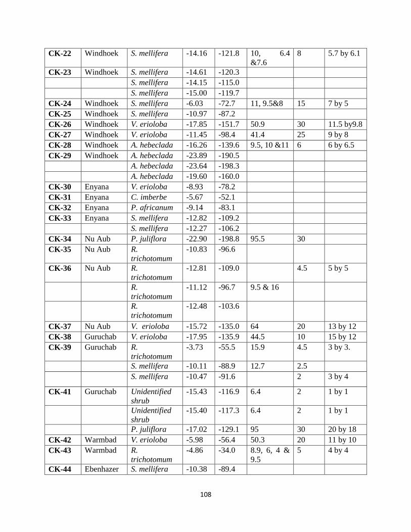
108

CK-22 Windhoek S. mellifera -14.16 -121.8 10, 6.4

&7.6

8 5.7 by 6.1

CK-23 Windhoek S. mellifera -14.61 -120.3

S. mellifera -14.15 -115.0

S. mellifera -15.00 -119.7

CK-24 Windhoek S. mellifera -6.03 -72.7 11, 9.5&8 15 7 by 5

CK-25 Windhoek S. mellifera -10.97 -87.2

CK-26 Windhoek V. erioloba -17.85 -151.7 50.9 30 11.5 by9.8

CK-27 Windhoek V. erioloba -11.45 -98.4 41.4 25 9 by 8

CK-28 Windhoek A. hebeclada -16.26 -139.6 9.5, 10 &11 6 6 by 6.5

CK-29 Windhoek A. hebeclada -23.89 -190.5

A. hebeclada -23.64 -198.3

A. hebeclada -19.60 -160.0

CK-30 Enyana V. erioloba -8.93 -78.2

CK-31 Enyana C. imberbe -5.67 -52.1

CK-32 Enyana P. africanum -9.14 -83.1

CK-33 Enyana S. mellifera -12.82 -109.2

S. mellifera -12.27 -106.2

CK-34 Nu Aub P. juliflora -22.90 -198.8 95.5 30

CK-35 Nu Aub R.

trichotomum

-10.83 -96.6

CK-36 Nu Aub R.

trichotomum

-12.81 -109.0 4.5 5 by 5

R.

trichotomum

-11.12 -96.7 9.5 & 16

R.

trichotomum

-12.48 -103.6

CK-37 Nu Aub V. erioloba -15.72 -135.0 64 20 13 by 12

CK-38 Guruchab V. erioloba -17.95 -135.9 44.5 10 15 by 12

CK-39 Guruchab R.

trichotomum

-3.73 -55.5 15.9 4.5 3 by 3.

S. mellifera -10.11 -88.9 12.7 2.5

S. mellifera -10.47 -91.6 2 3 by 4

CK-41 Guruchab Unidentified

shrub

-15.43 -116.9 6.4 2 1 by 1

Unidentified

shrub

-15.40 -117.3 6.4 2 1 by 1

P. juliflora -17.02 -129.1 95 30 20 by 18

CK-42 Warmbad V. erioloba -5.98 -56.4 50.3 20 11 by 10

CK-43 Warmbad R.

trichotomum

-4.86 -34.0 8.9, 6, 4 &

9.5

5 4 by 4

CK-44 Ebenhazer S. mellifera -10.38 -89.4

109

S. mellifera -8.80 -78.6

S. mellifera -9.97 -84.8

Table A.2: Groundwater isotopic composition.

Site δ18

O(‰)d18O δ2H(‰)d2H

Madisa -5.53 -42,.0

Sesfontein -7.60 -53.6

Fair Constantia -7.95 -63.1

Nu-Aub -5.89 -46.1

Guruchas -4.08 -30.5

Warmbad -5.69 -33.5

Ebenhazer -7.22 -53.6

Stinkwater -6.45 -42.5

SA2-1 -6.88 -51.2

SA2-4 -7.58 -54.2

SA2-14 -7.90 -56.9

Steinhausen -5.04 -38.8

Enyana -8.11 -59.2

Windhoek -6.77 -47.7