A Robust Method of Localization andMapping Using Only Range

Joseph Djugash, and Sanjiv Singh

The Robotics Institute, Carnegie Mellon University, Pittsburgh, PA 15213, USA{josephad, ssingh}@ri.cmu.edu

Summary. In this paper we present results in mobile robot localization and simul-taneous localization and mapping (SLAM) using range from radio. In previous workwe have shown how range readings from radio tags placed in the environment can beused to localize a robot and map tag locations using a standard extended Kalmanfilter (EKF) that linearizes the probability distribution due to range measurementsbased on prior estimates. Our experience with this method was that the filter couldperform poorly and even diverge in cases of missing data and poor initialization.Here we present a new formulation that gains robustness without sacrificing accu-racy. Specifically, our method is shown to have significantly better performance withpoor and even no initialization, infrequent measurements, and incorrect data associ-ation. We present results from a mobile robot equipped with high accuracy groundtruth, operating over several kilometers.

1 Motivation and Problem Statement

Here we focus on the problems of robust localization and SLAM given rangedata between a mobile robot and static “tags”. In the first case, the locations ofthe tags are known and the robot must accurately localize itself as it measuresrange to these tags while it moves. In the second case, the location of the tagsare not known ahead of time and must be determined in addition to beingused for localization. Hence our goal is to achieve a reliable and accurateestimate of pose for a robot operating in an environment containing radiotags to which the robot can measure range. This is a variant of a well knownproblem of SLAM for a robot using both range and bearing data to both mapan environment and localize itself.

Specifically, we would like a method that is robust to poor initialization,noise in measurement and missing data. We use three different datasets withover 2,000 range measurements each from a robot moving in a field of radiotags to compare the results from the proposed method to the classical standardEKF formulation. In each of the datasets, the robot travels over several km

and has highly accurate positioning for groundtruth. We find that our newmethod is more efficient, accurate and robust than the current standard.

2 Related Work

Most landmark-based localization systems use sensors that measure relativebearing or in some cases both range and bearing to distinct features in theenvironment. Of particular interest to us are those that use only range to lo-calize the network. For instance, the RADAR system, developed by Bahl andPadmanabhan, utilizes signal strength of packets in the commonly available802.11b wireless networks for localization of network devices [1]. However,signal strength measurements are often erratic and can be affected by slightchanges in the environment. Alternately, the Cricket system uses fixed ultra-sound emitters and embedded receivers in the target object to localize thetarget [2], [3]. Our system uses radio frequencies to measure range– as therobot moves, a transponder periodically sends out a query, and any tags thathear the query respond by sending a reply along with an unique ID number(trivially solving the correspondence problem). The robot can then estimatethe distance to each responding tag by determining the time lapsed betweensending the query and receiving the response.

Among others, Kantor et al. and Kurth et al. present single filter for-mulations to combine range measurements with dead reckoning and inertialmeasurements [4], [5]. These methods formulate the problem as an ExtendedKalman Filter (EKF) using linearization in the Euclidean space. Furthermore,these early efforts generally assume that the tag locations were approximatelyknown a priori. As can be expected with this formulation, the EKF solution isprone to problems of linearization and multi-modality, two issues particularlycommon when dealing with range only measurements. In some cases, rela-tively modest errors in the prior estimate of the tags and noisy measurementscan result in an incorrect estimate that will lead the filter to diverge. Theseissues have been dealt with in the fashion of typical EKF solutions: by assum-ing that the initial conditions (of the robot and the tag locations) specifiedare “pretty good” and that the noise in the measurements to be “normal”.Such assumptions are limiting and there is a need for a principled and robustmethod to use range data for localization and SLAM.

One such effort was presented by Leonard et al., in their use of a delayedstate filter [6]. This approach does not require any prior information about thelocations of the tags. Instead, a batch process on a set of collected measure-ments within a single EKF update step and allow the collected measurementsto identify the linearization point. The main drawback of such an approach isthe inability to determine when sufficient measurements have been collectedto safely linearize. More specifically, if the batch update chooses the incorrectof the multiple hypotheses due to the lack of sufficient measurements, it isnear impossible for the filter to recover from that error. Alternately, Olson et

al. proposed the use of a separate pre-filtering step to approximately locatethe landmarks/tags and identify the linearization point [7]. The pre-filteringstep involves the use of a hough transform that identifies peaks within thelikelihood distribution for a tag, given a collection of measurements. By de-laying the initialization of a tag until the hough transform identifies a singlepeak with a significantly higher likelihood, the method is able to determine,in an online manner, the exact size of the measurement set needed to achievea good initialization. While this approach seems adequate at first glance, inthe presence of large measurement/odometric error and sparse data the peakswithin the hough transform become blurred and form a “ridge”. This blurringforces the initialization of the tag to be delayed, and with sufficient odometryerror it is possible that the distribution never converges to a single peak.

Previously, we have also investigated the use of other filters to address theproblem of range-only SLAM [8], [9]. One such method, Monte Carlo localiza-tion, or particle filtering, provides a method of representing multimodal dis-tributions for position estimation, with the advantage that the computationalrequirements can be scaled. However, these sample based methods becomeintractable (for real-time applications) when modeling the cross-correlationterms sometimes necessary in SLAM. If the particle count in reduced to main-tain real-time computation, particle depletion then causes the filter to diverge.

While majority of prior research has focused on formulating the problem inthe Euclidean space, we propose the use of a polar parameterization to moreaccurately represent the nonlinear distributions encountered in the range-onlySLAM. This parameterization is similar to one proposed by Funiak et al. [10]for a very different problem– tracking targets from camera networks where thelocations and orientations of the cameras are not known. They demonstratethe use of polar parameterization to model the annulus-like distributions thatoccur while estimating the pose of a camera observing a mobile target evenwith bearing-only measurements. Civera et al. also address a similar prob-lem in monocular SLAM where they utilize a hybrid estimation scheme todeal with the nonlinear distributions that occur when the camera is eitherstationary or rotating for significant period of time [11].

Unlike much of the existing methods that linearize the measurements inthe Euclidean space, the proposed method operates in the polar space wherethe linearization is much improved. As such, our method does not require aprior nor does it perform a batch process to identify the linearization point.In addition, the proposed method is also able to model the multi-modal dis-tributions that naturally occur with range measurements.

3 Technical Approach

In the following sections, we present the formulation of the proposed methodand compare its results to the standard EKF that has been previously testedand proven. First, we present a quick overview of the standard EKF, which

linearizes the range measurements in the Euclidean space. Then, we detail ourproposed method, the relative-over parametrized (ROP) EKF, using the newparametrization tailored to represent range data.

The basic intuition behind the ROP-EKF is that the distributions re-sulting from range measurement can be more faithfully represented if thelinearization of the range measurements is done in polar coordinates insteadof Cartesian coordinates. In addition since multiple modes naturally arise inthe distributions after multiple measurements, our method includes means formaintaining multiple hypotheses. Lastly, we compare the results of the pro-posed method against the standard EKF, using real-world experimental data(Section 4) in the area of the size of a football field.

3.1 The Standard EKF

The standard EKF is formulated to estimate the position of the mobile ro-bot given measurements of odometry (from wheel encoders), heading change(from a gyro), and range measurements to stationary tags in the environment.Odometry and gyro measurements are used in the state propagation or theprediction step, while the range measurements are incorporated in the correc-tion step. The method presented here is used as a baseline comparison for ourproposed method described in Section 3.2.

Let the robot state (position and orientation) at time k be represented bythe state vector qk = [xr

k, yrk, φr

k]T . The dynamics of the wheeled robot used inthe experiments are best described by the following set of nonlinear equations:

qk+1 =

xrk +4Dk cos(φr

k)yr

k +4Dk sin(φrk)

φrk +4φk

+ νk = f(qk, uk) + νk, (1)

where νk is a noise vector, 4Dk is the odometric distance traveled, and4φk is the orientation change. For every new control input vector, u(k) =[4Dk,4φk]T , that is received, the estimates of robot state and error co-variance are propagated using the extended Kalman filter (EKF) predictionequations.

The range measurement received at time k is modeled by:

rbk =

√(xr

k − xbk)2 + (yr

k − ybk)2 + ηk (2)

where, rbk is the estimate of the range from the tag to the current state, (xb

k, ybk)

is the location of the tag from which the measurement was received and ηk iszero mean Gaussian noise. The measurement is linearized and incorporatedinto the state and covariance estimates using the EKF update equations.

When performing SLAM, we extend the state vector to include the positionestimates of each tag. Thus we get,

qk =[xr

k, yrk, φr

k, x1k, y1

k, ... xNk , yN

k

]T (3)

Fig. 1. True and approximated distributions with one range observation (Top Row)and two observations from different locations (Bottom Row). True distributions inCartesian coordinates (Left Column), true and Gaussian approximated distributionsin polar coordinates (Middle Column), and projection of the Gaussian approximateddistribution into Cartesian coordinates. In these figures, blue squares represent ob-serving tags, whose location is known. Red diamonds represent the true locationof the observed tag, whose position is being estimated and green circles representthe mean(s) for each mode of the estimated tag. Green shaded regions representthe true uncertainty distribution and blue ellipses represent the estimated uncer-tainty distribution. The dashed gray lines and circles represent the observed rangemeasurements.

where n is the number of initialized tags at time k. The motion model for thefirst three states is given by ( 1). The tags do not move, so the motion modelfor the remaining states is trivial. The measurement model is the same as thatstated in ( 2) with xb

k and ybk replaced by xi

k and yik when the measurement

is received from the ith tag.When no prior knowledge of the tag locations exist, it is necessary to per-

form some type of batch process to initialize tag locations, which are thenrefined within the filter. We employ an approach similar to [7] that utilizes atwo-dimensional probability grid to provide initial estimates of the tag loca-tions. Here a “voting” scheme is used to identify likely locations of the tags,the cells with the greatest number of votes.

3.2 ROP-EKF: Relative-Over Parameterization

While the standard EKF described above operates in the Euclidean space,we formulate our problem in polar coordinates. At each time step, k, thestate of tag i is represented by qi

k = [cix,k, ci

y,k, rik, θi

k]T . Each tag’s estimateis represented in a polar coordinates, where (ci

x,k, ciy,k) are the center of the

polar coordinate frame and (rik, θi

k) are the corresponding range and anglevalues. The use of this parameterization derives motivation from the polarcoordinate system, where annuli, crescents and other ring-like shapes can beeasily modeled. In addition to the four variable relative-over parameterization,for the mobile robot, an addition term that represents the current heading ofthe robot, φr

k, is maintained. Thus, the complete state vector at time k isrepresented as:

qk = [qrk, φr

kq1k, q2

k, ..., qNk ]T .

where N is the total number of tags. At each time step, we get some set ofmotion and range observations, uk and zk respectively.

While the motion model remains the same as described in (1), only the(cr

x,k, cry,k) terms of the robot’s state are updated. The remaining terms,

(rrk, θr

k, are left unchanged by the motion update. The measurement model,however, requires a slight change to equation 2. In order to compute the ex-pected range using the (xi

k, yik) of the robot/tag, we need to first transform

their positions from the polar coordinates into the Cartesian coordinates:

xik = ci

x,k + rik · cos(θi

k).yi

k = ciy,k + ri

k · sin(θik). (4)

The range measurements can now be incorporated into the state and co-variance estimates using the EKF update equations. The measurement matrixfor the polar parameterization, used in the EKF update, is given by the Ja-cobian H:

H = ∂ri

∂qr =

(xr−xi)zri

(yr−yi)zri

cos(θr) (xr−xi)zri

+ sin(θr) (yr−yi)zri

rr(cos(θr) (yr−yi)zri

− sin(θr) (xr−xi)zri

)

zri =√

(xr − xi)2 + (yr − yi)2

(5)

Unlike the standard EKF formulation, the relative-over parameterizedEKF does not require a separate batch process to initialize the tags withinthe filter. Instead, upon the first observation of a particular tag, the annulusof the true distribution is approximated by an elongated Gaussian in polarcoordinates (rθ-space). This Gaussian approximation is given an arbitrarymean in θ (within the range [0, 2π)) with a large variance term, such that the

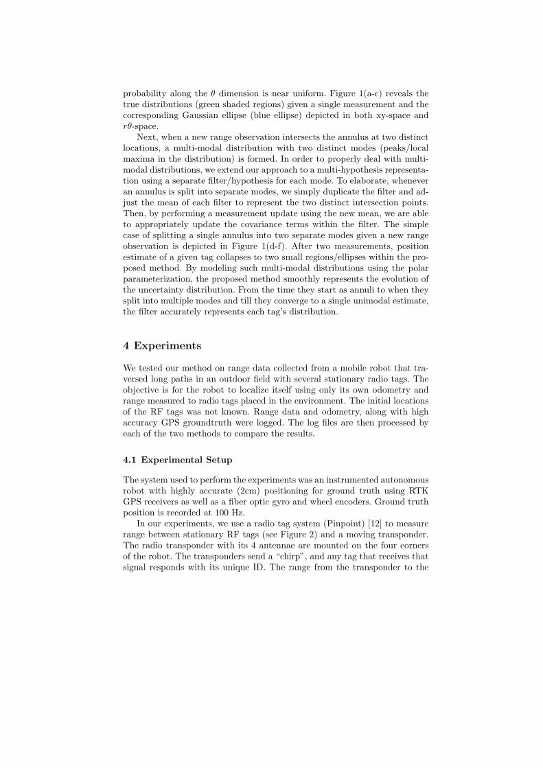
probability along the θ dimension is near uniform. Figure 1(a-c) reveals thetrue distributions (green shaded regions) given a single measurement and thecorresponding Gaussian ellipse (blue ellipse) depicted in both xy-space andrθ-space.

Next, when a new range observation intersects the annulus at two distinctlocations, a multi-modal distribution with two distinct modes (peaks/localmaxima in the distribution) is formed. In order to properly deal with multi-modal distributions, we extend our approach to a multi-hypothesis representa-tion using a separate filter/hypothesis for each mode. To elaborate, wheneveran annulus is split into separate modes, we simply duplicate the filter and ad-just the mean of each filter to represent the two distinct intersection points.Then, by performing a measurement update using the new mean, we are ableto appropriately update the covariance terms within the filter. The simplecase of splitting a single annulus into two separate modes given a new rangeobservation is depicted in Figure 1(d-f). After two measurements, positionestimate of a given tag collapses to two small regions/ellipses within the pro-posed method. By modeling such multi-modal distributions using the polarparameterization, the proposed method smoothly represents the evolution ofthe uncertainty distribution. From the time they start as annuli to when theysplit into multiple modes and till they converge to a single unimodal estimate,the filter accurately represents each tag’s distribution.

4 Experiments

We tested our method on range data collected from a mobile robot that tra-versed long paths in an outdoor field with several stationary radio tags. Theobjective is for the robot to localize itself using only its own odometry andrange measured to radio tags placed in the environment. The initial locationsof the RF tags was not known. Range data and odometry, along with highaccuracy GPS groundtruth were logged. The log files are then processed byeach of the two methods to compare the results.

4.1 Experimental Setup

The system used to perform the experiments was an instrumented autonomousrobot with highly accurate (2cm) positioning for ground truth using RTKGPS receivers as well as a fiber optic gyro and wheel encoders. Ground truthposition is recorded at 100 Hz.

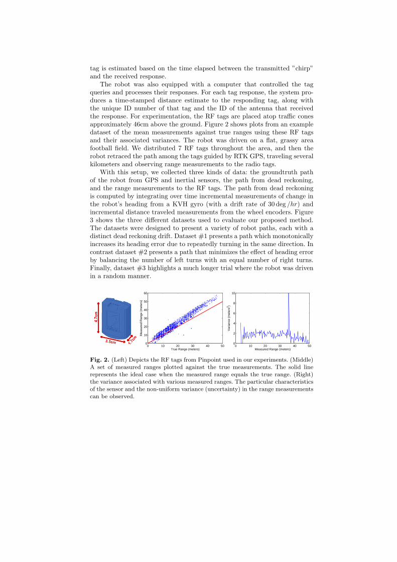
In our experiments, we use a radio tag system (Pinpoint) [12] to measurerange between stationary RF tags (see Figure 2) and a moving transponder.The radio transponder with its 4 antennae are mounted on the four cornersof the robot. The transponders send a “chirp”, and any tag that receives thatsignal responds with its unique ID. The range from the transponder to the

tag is estimated based on the time elapsed between the transmitted ”chirp”and the received response.

The robot was also equipped with a computer that controlled the tagqueries and processes their responses. For each tag response, the system pro-duces a time-stamped distance estimate to the responding tag, along withthe unique ID number of that tag and the ID of the antenna that receivedthe response. For experimentation, the RF tags are placed atop traffic conesapproximately 46cm above the ground. Figure 2 shows plots from an exampledataset of the mean measurements against true ranges using these RF tagsand their associated variances. The robot was driven on a flat, grassy areafootball field. We distributed 7 RF tags throughout the area, and then therobot retraced the path among the tags guided by RTK GPS, traveling severalkilometers and observing range measurements to the radio tags.

With this setup, we collected three kinds of data: the groundtruth pathof the robot from GPS and inertial sensors, the path from dead reckoning,and the range measurements to the RF tags. The path from dead reckoningis computed by integrating over time incremental measurements of change inthe robot’s heading from a KVH gyro (with a drift rate of 30 deg /hr) andincremental distance traveled measurements from the wheel encoders. Figure3 shows the three different datasets used to evaluate our proposed method.The datasets were designed to present a variety of robot paths, each with adistinct dead reckoning drift. Dataset #1 presents a path which monotonicallyincreases its heading error due to repeatedly turning in the same direction. Incontrast dataset #2 presents a path that minimizes the effect of heading errorby balancing the number of left turns with an equal number of right turns.Finally, dataset #3 highlights a much longer trial where the robot was drivenin a random manner.

0 10 20 30 40 500

10

20

30

40

50

60

True Range (meters)

Mea

sure

d R

ange

(m

eter

s)

0 10 20 30 40 500

2

4

6

8

10

Measured Range (meters)

Var

ianc

e (m

eter

s2 )

Fig. 2. (Left) Depicts the RF tags from Pinpoint used in our experiments. (Middle)A set of measured ranges plotted against the true measurements. The solid linerepresents the ideal case when the measured range equals the true range. (Right)the variance associated with various measured ranges. The particular characteristicsof the sensor and the non-uniform variance (uncertainty) in the range measurementscan be observed.

−10 0 10 20 30 40 50 60

0

20

40

60

80

100

120

y position (m)

x po

sitio

n (m

)

483

125

266

201

1226

113

322

Ground TruthOdometryTrue Tag Loc.

−10 0 10 20 30 40 50 60

0

20

40

60

80

100

120

y position (m)

x po

sitio

n (m

)

342

76

284

136

980

136

100

Ground TruthOdometryTrue Tag Loc.

−10 0 10 20 30 40 50 60

0

20

40

60

80

100

120

y position (m)

x po

sitio

n (m

)

1626

564

789

1074

3978

1125

429

Ground TruthOdometryTrue Tag Loc.

Fig. 3. The robot’s true path is shown in blue along with its dead reckoning positionin green and the true tag locations for three different datasets. The numbers next toeach tag presents the number of measurements received by the robot from the tag.(Left) Dataset #1: the robot traveled 3.7 km receiving 2749 range measurements.(Middle) Dataset #2: the robot traveled 1.36 km receiving 2146 range measurements.(Right) Dataset #3: the robot traveled 6.7 km receiving 10068 range measurements.To reduce the clutter only the initial 1km of the path is shown, however, the fulldataset is evaluated and compared numerically.

4.2 Results

Table 1 shows robot path and tag mapping errors from performing localizationand SLAM with the two different methods described above. The table revealsthat for localization the proposed ROP-EKF performs better. While in SLAMon dataset #1 it produces a higher robot path error, the tag mapping errorsare much improved over the standard EKF. Additionally, it should be notedthat when comparing the SLAM results it is best to observe errors in thefinal segment (we report the path errors over the final 10%) of the robotpath, instead of the full robot path to illustrate the performance after thetag locations have converged. Note that heuristically we stop updating thelocation of the tags once their uncertainty falls below a threshold (0.3 m inthe experiments described). This has the effect of only updating the position ofthe robot and the other tags (via the covariances) when range measurementsare received. Figure 4 shows the output of the proposed ROP-EKF SLAM oneach of the three datasets along with the robot path error over time.

The raw result from SLAM does not produce a globally aligned solution,since no reference coordinate frame is provided apriori to fix the map (locationof the tags). Hence a simple affine transform (consisting of only a rotationaland translational components) needs to be performed on both the map andpath estimates. The transform that is applied, is one that best aligns the esti-mated map to the real ground truth surveyed map. This produces a reasonablemetric by which we can evaluate the accuracy of the SLAM solution.

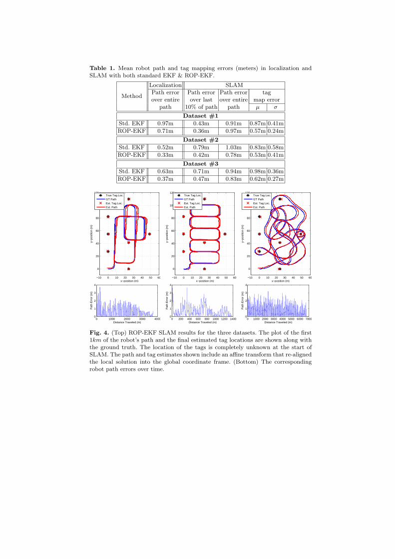
Table 1. Mean robot path and tag mapping errors (meters) in localization andSLAM with both standard EKF & ROP-EKF.

Method

Localization SLAMPath error Path error Path error tagover entire over last over entire map error

path 10% of path path µ σ

Dataset #1

Std. EKF 0.97m 0.43m 0.91m 0.87m 0.41m

ROP-EKF 0.71m 0.36m 0.97m 0.57m 0.24m

Dataset #2

Std. EKF 0.52m 0.79m 1.03m 0.83m 0.58m

ROP-EKF 0.33m 0.42m 0.78m 0.53m 0.41m

Dataset #3

Std. EKF 0.63m 0.71m 0.94m 0.98m 0.36m

ROP-EKF 0.37m 0.47m 0.83m 0.62m 0.27m

−10 0 10 20 30 40 50 60

0

20

40

60

80

100

120

x−position (m)

y−po

sitio

n (m

)

True Tag Loc.GT PathEst. Tag Loc.Est. Path

0 1000 2000 3000 40000

1

2

3

4

Distance Traveled (m)

Pat

h E

rror

(m

)

−10 0 10 20 30 40 50 60

0

20

40

60

80

100

120

x−position (m)

y−po

sitio

n (m

)

True Tag Loc.GT PathEst. Tag Loc.Est. Path

0 200 400 600 800 1000 1200 14000

1

2

3

4

Distance Traveled (m)

Pat

h E

rror

(m

)

−10 0 10 20 30 40 50 60

0

20

40

60

80

100

120

x−position (m)

y−po

sitio

n (m

)

True Tag Loc.GT PathEst. Tag Loc.Est. Path

0 1000 2000 3000 4000 5000 6000 70000

1

2

3

4

Distance Traveled (m)

Pat

h E

rror

(m

)

Fig. 4. (Top) ROP-EKF SLAM results for the three datasets. The plot of the first1km of the robot’s path and the final estimated tag locations are shown along withthe ground truth. The location of the tags is completely unknown at the start ofSLAM. The path and tag estimates shown include an affine transform that re-alignedthe local solution into the global coordinate frame. (Bottom) The correspondingrobot path errors over time.

Initialization

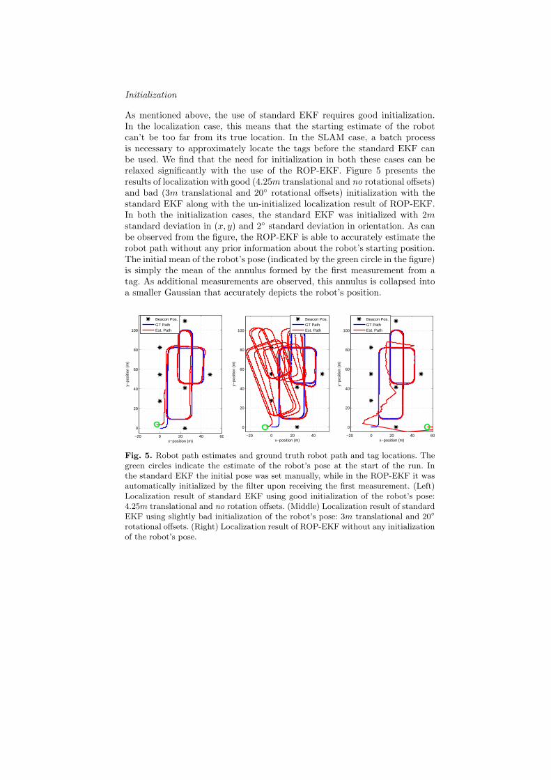
As mentioned above, the use of standard EKF requires good initialization.In the localization case, this means that the starting estimate of the robotcan’t be too far from its true location. In the SLAM case, a batch processis necessary to approximately locate the tags before the standard EKF canbe used. We find that the need for initialization in both these cases can berelaxed significantly with the use of the ROP-EKF. Figure 5 presents theresults of localization with good (4.25m translational and no rotational offsets)and bad (3m translational and 20◦ rotational offsets) initialization with thestandard EKF along with the un-initialized localization result of ROP-EKF.In both the initialization cases, the standard EKF was initialized with 2mstandard deviation in (x, y) and 2◦ standard deviation in orientation. As canbe observed from the figure, the ROP-EKF is able to accurately estimate therobot path without any prior information about the robot’s starting position.The initial mean of the robot’s pose (indicated by the green circle in the figure)is simply the mean of the annulus formed by the first measurement from atag. As additional measurements are observed, this annulus is collapsed intoa smaller Gaussian that accurately depicts the robot’s position.

−20 0 20 40 60

0

20

40

60

80

100

x−position (m)

y−po

sitio

n (m

)

Beacon Pos.GT PathEst. Path

−20 0 20 40

0

20

40

60

80

100

x−position (m)

y−po

sitio

n (m

)

Beacon Pos.GT PathEst. Path

−20 0 20 40 60

0

20

40

60

80

100

x−position (m)

y−po

sitio

n (m

)

Beacon Pos.GT PathEst. Path

Fig. 5. Robot path estimates and ground truth robot path and tag locations. Thegreen circles indicate the estimate of the robot’s pose at the start of the run. Inthe standard EKF the initial pose was set manually, while in the ROP-EKF it wasautomatically initialized by the filter upon receiving the first measurement. (Left)Localization result of standard EKF using good initialization of the robot’s pose:4.25m translational and no rotation offsets. (Middle) Localization result of standardEKF using slightly bad initialization of the robot’s pose: 3m translational and 20◦

rotational offsets. (Right) Localization result of ROP-EKF without any initializationof the robot’s pose.

Bad Correspondence

While our sensor system trivially solves the correspondence problem by send-ing an unique ID along with the transmitted signal, we show how this methodperforms even if the data association is significantly degraded by artificiallycorrupting data association. Figure 6 presents the tag mapping errors of SLAMusing both the methods described above for increasing percentages of incor-rect data association. We note that even with severe errors in data association,the ROP-EFK maps tags with relatively high accuracy. Figure 7 shows thatthe path error of the two methods is comparable when the data association isperfect but that the ROP-EKF is significantly better in estimating paths inthe presence of significant data association error.

0 10 20 30 40 500

5

10

15

20

25

30

35

40

45

% of Meas. with Incorrect Data Association

Mea

n T

ag M

appi

ng E

rror

(m

)

Std. EKFROP−EKF

Fig. 6. Mean tag mapping errors ofSLAM using both the methods de-scribed above for increasing amount ofmeasurements with incorrect data asso-ciations.

0 1000 2000 3000 4000 0.

1.

2.

3.

4.

Rob

ot P

ath

Err

or (

m) Std. EKF w/ Perfect DA

ROP−EKF w/ Perfect DA

0 1000 2000 3000 40000

10

20

30

Time

Rob

ot P

ath

Err

or (

m) Std. EKF 20% DA error

ROP−EKF 30% DA error

Fig. 7. Mean path error over timefor two cases of SLAM (Top) perfectdata association (DA) for both methods.(Bottom) 20% incorrect DA with Std.EKF in blue and 30% incorrect DA withROP-EKF in red.

Sparse Data

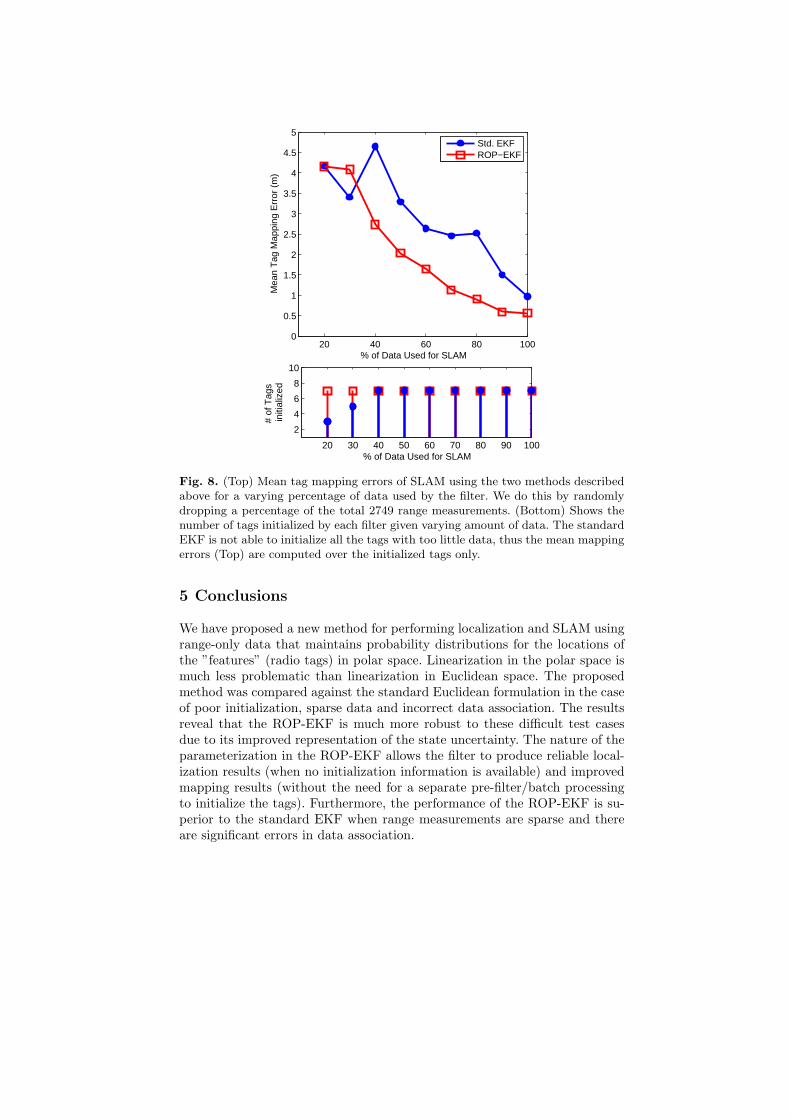
In the final evaluation, we examined the performance with a varying amount ofinput data. We do this by randomly dropping a percentage of the range mea-surements. Figure 8 shows that the ROP-EKF consistently maps the tags withhigher accuracy (50-100%) than the standard EKF. With extremely sparsedata (≤ 30% of the dataset), both methods performs poorly. This is becausewith few measurements, postions of tags are underconstrained and the robot’sestimate of its own position drifts with odometric errors.

20 40 60 80 1000

0.5

1

1.5

2

2.5

3

3.5

4

4.5

5

% of Data Used for SLAM

Mea

n T

ag M

appi

ng E

rror

(m

)

Std. EKFROP−EKF

20 30 40 50 60 70 80 90 100

2

4

6

8

10

% of Data Used for SLAM

# of

Tag

s in

itial

ized

Fig. 8. (Top) Mean tag mapping errors of SLAM using the two methods describedabove for a varying percentage of data used by the filter. We do this by randomlydropping a percentage of the total 2749 range measurements. (Bottom) Shows thenumber of tags initialized by each filter given varying amount of data. The standardEKF is not able to initialize all the tags with too little data, thus the mean mappingerrors (Top) are computed over the initialized tags only.

5 Conclusions

We have proposed a new method for performing localization and SLAM usingrange-only data that maintains probability distributions for the locations ofthe ”features” (radio tags) in polar space. Linearization in the polar space ismuch less problematic than linearization in Euclidean space. The proposedmethod was compared against the standard Euclidean formulation in the caseof poor initialization, sparse data and incorrect data association. The resultsreveal that the ROP-EKF is much more robust to these difficult test casesdue to its improved representation of the state uncertainty. The nature of theparameterization in the ROP-EKF allows the filter to produce reliable local-ization results (when no initialization information is available) and improvedmapping results (without the need for a separate pre-filter/batch processingto initialize the tags). Furthermore, the performance of the ROP-EKF is su-perior to the standard EKF when range measurements are sparse and thereare significant errors in data association.

6 Acknowledgments

This work is supported by the National Science Foundation under Grant No.IIS-0426945.

References

1. P. Bahl and V. Padmanabhan, “Radar: An in-building RF-based user locationand tracking system,” in In Proc. of the IEEE Infocom 2000, Tel Aviv, Israel,March 2000.

2. N. Priyantha, A. Chakraborty, and H. Balakrishman, “The cricket location sup-port system,” in In Proc. of the 6th Annual ACM/IEEE International Confer-ence on Mobile Computing and Networking (MOBICOM 2000), Boston, MA,August 2000.

3. A. Smith, H. Balakrishnan, M. Goraczko, and N. B. Priyantha, “Tracking Mov-ing Devices with the Cricket Location System,” in 2nd International Conferenceon Mobile Systems, Applications and Services (Mobisys 2004), Boston, MA,June 2004.

4. G. Kantor and S. Singh, “Preliminary results in range-only localization andmapping,” Robotics and Automation, 2002. Proceedings. ICRA’02. IEEE Inter-national Conference on, vol. 2, 2002.

5. D. Kurth, G. Kantor, and S. Singh, “Experimental results in range-only local-ization with radio,” Intelligent Robots and Systems, 2003.(IROS 2003). Pro-ceedings. 2003 IEEE/RSJ International Conference on, vol. 1, 2003.

6. J. Leonard, R. Rikoski, P. Newman, and M. Bosse, “Mapping partially observ-able features from multiple uncertain vantage points.” International Journal ofRobotics Research, vol. 21, no. 10, pp. 943–975, 2002.

7. E. Olson, J. Leonard, and S. Teller, “Robust range-only beacon localization,”in Proceedings of Autonomous Underwater Vehicles, 2004, 2004.

8. J. Djugash, S. Singh, and P. I. Corke, “Further results with localization andmapping using range from radio,” in International Conference on Field & Ser-vice Robotics, July 2005.

9. J. Djugash, S. Singh, G. Kantor, and W. Zhang, “Range-only slam for robotsoperating cooperatively with sensor networks,” in IEEE Int’l Conf. on Roboticsand Automation (ICRA ‘06), 2006.

10. S. Funiak, C. E. Guestrin, R. Sukthankar, and M. Paskin, “Distributed localiza-tion of networked cameras,” in Fifth International Conference on InformationProcessing in Sensor Networks (IPSN’06), April 2006, pp. 34 – 42.

11. J. Civera, A. Davison, and J. Montiel, “Interacting multiple model monocularslam,” in IEEE International Conference on Robotics and Automation, May2008.

12. J. Werb and C. Lanzl, “Designing a positioning system for finding things andpeople indoors,” Spectrum, IEEE, vol. 35, no. 9, pp. 71–78, 1998.