Ann. Telecommun. manuscript No.(will be inserted by the editor)

A Non-Coherent Architecture for GNSS Digital Tracking Loops

Daniele Borio · Gerard Lachapelle

the date of receipt and acceptance should be inserted later

Abstract In this paper a new non-coherent architecture forGNSS tracking loops is proposed and analyzed. A non-coherentphase discriminator, able to extend the integration time be-yond the bit duration is derived from the Maximum Like-lihood principle and integrated into a Costas loop. The dis-criminator is non-coherent in the sense that the bit informa-tion is removed by using a non-linear operation. By jointlyusing such a discriminator and non-coherent integrations atthe Delay Lock Loop level, a fully non-coherent architec-ture, able to operate at low carrier-power-to-noise density ra-tio (C/N0), is obtained. The algorithms proposed have beentested by means of live GPS data and compared with ex-isting methodologies, resulting in an effective solution forextending the total integration time.

Keywords Coherent Integration, Global Navigation Satel-lite System, GNSS, Long Integration, Loop Discriminators,Non-coherent Integration, Tracking Loops, Weak signals

1 Introduction

The continuous development of High-Sensitivity Global Nav-igation Satellite System (HSGNSS) receivers is making pos-sible the acquisition and tracking of signals attenuated byapproximatively 30 dB [1]. Those impressive results are gen-erally obtained by extending the integration time and suc-cessfully compensating for the user dynamic and the effectof the navigation message. In this way a HSGNSS receiver is

Daniele Borio and Gerard LachapelleUniversity of Calgary, Department of Geomatics Engineering2500 University Dr NWCalgary, Alberta, T2N 1N4 CanadaTel.: +1-403-2109797E-mail: dborio@ucalgary.caE-mail: lachapel@ucalgary.ca

able to provide an increased processing gain that allows thesuccessful recovery of weak and extremely weak signals.The extension of the integration time, at both acquisition andtracking levels, allows one to average out the noise compo-nents and to reduce the effect of Radio Frequency (RF) in-terference. Long integrations can be achieved by means ofeither coherent or non-coherent processing. The former pro-vides increased performance in term of noise reduction, atthe cost of vulnerability to frequency errors and bit transi-tions in the navigation message. Non-coherent processingconsists of applying a non-linear transformation to the inputsignal, removing the effects of data transitions and reducingthe impact of frequency errors. This non-linear transforma-tion generally amplifies the noise impact, incurring in the socalled squaring loss [2, 3].At the tracking level, particular attention has been devotedto the development of specific techniques for coherently in-creasing the integration time [1,4–9]. More specifically, dif-ferent techniques have been adopted to detect a bit transitionand compensate its effect during the coherent integrationprocess. In general an initial synchronization is assumed andthe bit boundaries are supposed to be known. Thus the inputsignal is at first integrated over the bit duration and the polar-ity of each block is determined using different techniques [5,7]. Although non-coherent integrations are commonly usedfor acquiring weak signals [10], non-coherent processinghas been only marginally considered for extending the in-tegration time at the tracking level. In the context of signalacquisition [11, 12] it has been shown that, for low carrier-power-to-noise density ratio (C/N0), non-coherent integra-tion outperforms coherent processing with bit recovery. Thismerely illustrates the fact that relative bit sign recovery be-comes unreliable at low C/N0. A similar phenomena is alsoexpected for tracking loops that rely on bit estimation: forlow C/N0 bit estimation becomes unreliable and non-coherentprocessing should be preferred. For this reasons the main

2

topic of this paper is the design and analysis of loop dis-criminators that non-coherently extend the integration timein tracking loops. Specific focus has been devoted to the de-sign of a non-coherent Phase Lock Loop (PLL) with longintegration capability. The carrier phase discriminator hasbeen obtained by evaluating the Maximum Likelihood (ML)estimator for the common phase of a set of data blocks mod-ulated by an unknown bit sequence. The expression for theML phase estimator in the presence of bit transitions was al-ready considered, in a different context, by [6] for initializ-ing a Kalman filter based tracking loop. However, to the bestof the authors’ knowledge, this estimator was never used asnon-coherent discriminator for a PLL and thus it representsone of the innovative contributions of this paper. The codediscriminator has been obtained by using a non-coherentversion of the correlation as cost function the code track-ing loop is trying to maximize. Although this last approachcan be directly derived from non-coherent integrations foracquisition and it has been already considered in the litera-ture [13], it allows the design of a fully non-coherent HS-GNSS receiver.The obtained non-coherent architecture has been comparedwith existing methodologies, where the integration time iscoherently extended by estimating the received bits. Bothcoherent and non-coherent architectures have been imple-mented in the University of Calgary’s GNSS Software Nav-igation Receiver (GSNRxT M) [14] and tested by using liveGPS data. The integration time as been extended till 80 msand the loop filters have been designed by using a controlled-root formulation [15]. The proper filter design and the use ofnon-coherent integrations have led to a stable GNSS receiverable to operate in weak signal conditions. From the analysisthe non-coherent architecture results in an effective alterna-tive to coherent integrations enabling less noisy measure-ments than the ones obtained by means of standard loops.The remainder of this paper is organized as follows: in Sec-tion 2 the signal model is defined and the basic principles ofGNSS tracking loops established. In Section 3 the ML phaseestimator is derived and the non-coherent PLL and DLL dis-criminators defined. In Section 4 the approach for extendedcoherent integrations is briefly summarized. Section 5 dealswith the linear loop model and filter design whereas Section6 analyzes the tracking jitter for the non-coherent and coher-ent cases. In Section 7 real data are used to demonstrate theuse of the proposed architecture. Section 8 suggests a fur-ther extension of the proposed discriminators and, finally,the conclusions are addressed in Section 9.

2 Signal and system model

The complex baseband signal at the input of a digital track-ing loop, in a one-path additive Gaussian noise environment,

can be expressed as the sum of a useful signal and a noiseterm:

s[n] = y[n]+w[n]

= Ad[n− τ0/Ts]c[n− τ0/Ts]exp{ jθ [n]}+w[n](1)

where c[n] is the signal spreading sequence and d[n] is thenavigation message, that, for the GPS C/A modulation, makesthe polarity of the received signal change each 20 ms. τ0 isthe delay experienced by the received signal (modulo 1 ms)and θ [n] is, in general, a time varying process that modelsthe phase and frequency errors that have to be recovered bythe PLL. A is the signal amplitude that also accounts for theeffect of the Automatic Gain Control (AGC) before analogto digital conversion. w[n] is a zero mean complex Gaussianprocess whose statistical properties depend on the decima-tion and filtering strategies adopted at the front-end level.s[n] is a discrete time process obtained by sampling the con-tinuous time signal s(t) at the sampling frequency fs = 1

Ts.

In the remainder of this paper, the notation s[n] = s(nTs) isadopted for denoting sampled signals.It is noted that the signal recovered by a GNSS receiver isusually made up of several components transmitted by dif-ferent satellites. However, due to the quasi-orthogonality ofthe different spreading sequences, the different useful sig-nals are analyzed separately by the receiver, thus justifying(1).In GNSS receivers the code delay, τ0, and residual phase,θ [n], are usually estimated by two separate tracking loops:the DLL and the PLL/FLL. The main focus of this paper isthe design of a PLL discriminator employing non-coherentintegrations for extending the total integration time beyondthe bit duration. For this reason the DLL is only marginallyconsidered and perfect code delay synchronization is as-sumed. Under the assumption of perfect code synchroniza-tion and after code wipe-off, the input signal (1) becomes

r[n] = Ad[n− τ0/Ts]exp{ jθ [n]}+w′[n] (2)

where the code dependence has been removed by the use-ful signal and w′[n] = w[n]c[n− τ0/Ts] is a complex Gaus-sian process characterized by the same mean and variance ofw[n]. In Fig. 1 the scheme of the standard PLL is depicted.In this case bit transitions are neither recovered nor elimi-nated and the integration time is limited by the bit duration.The signal r[n] is correlated with a local carrier replica andthe correlator output is used to evaluate an estimate of theresidual phase, through a non-linear discriminator. The dis-criminator output is then filtered and used to drive the Nu-merically Controlled Oscillator (NCO) for the local carriergeneration. In Fig.1, N denotes the number of samples usedfor evaluating the correlation between the local and receivedsignal. The complex correlator output can be modeled as fol-lows [16]:

P = PI + jPQ = dAc exp{ jφ}+ηP (3)

3

Non-linear discriminator

( )F zLoop Filter

NCO

Carrier generator

1

0

1 ( )N

nN

−

=

⋅∑[ ]r n

Integrate & Dump: Coherent Integration

N

Fig. 1 Scheme of a standard PLL.

where

– d models the effect of the navigation message, assumedconstant during the coherent integration process;

– Ac is the amplitude of the correlator output, also account-ing for the losses introduced by residual frequency er-rors;

– φ is a residual phase error that will be extracted by thenon-linear discriminator;

– ηP is a complex Gaussian random variable derived byprocessing the noise term w′[n].

A common choice in the literature [16] is to assume that theinput signal r[n] has been normalized such that the real andimaginary parts of ηP have unit variance. This choice doesnot affect the results reported herein since the power rela-tionship between signal and noise are preserved by scaling.Under this condition and neglecting the impact of front-endfiltering and frequency errors, it is possible to show [16] that

Ac =√

2C/N0T (4)

where C/N0 is the carrier-power-to-noise density ratio [17]and T = NTs is the coherent integration time. It is notedthat a more complex model, accounting for front-end fil-tering and the presence of non-white interference, can beadopted [18, 19]. More specifically, the C/N0 in (4) shouldbe substituted by the effective C/N0, introduced by [20, 21]when accounting for several signal imperfections.When considering PLL with extended integration time, sev-eral correlator outputs, obtained from subsequent portionsof the input signal, are evaluated and used for producingan improved phase estimate. For this reason, the index k =0,1, ...,K − 1 is introduced and the different correlator out-puts are denoted as

Pk = PI,k + jPQ,k = dkAc exp{ jφ}+ηP,k. (5)

In (5) the quantities {dk}K−1k=0 are modeled as independent

random variables assuming values from the set {−1,1} with

equal probability. The phase error, φ , and the correlator out-put amplitude are assumed constant for all k, whereas therandom variables

{ηP,k}K−1

k=0 are considered independent andidentically distributed (i.i.d.). Eq. (5) represents the basicsignal model adopted in the paper.

3 Non-coherent discriminators

In standard Costas loops, the discriminator is obtained byconsidering the correlator output model (3) and deriving theMaximum Likelihood (ML) estimator for the phase error φ

[17]. More specifically, the arctangent discriminator

S = arctan(

PQ

PI

)(6)

is the ML phase estimator [17] when considering only onecomplex correlator output. Other discriminators can be ob-tained by using different approximations for the arctangentfunction. In this section the phase ML estimator, when con-sidering model (5) and the availability of K correlator out-puts, is at first derived and used for the design of a new phasediscriminator. A discriminator for non-coherently extendingthe integration time into a DLL is also introduced in Section3.3.

3.1 ML phase estimator

When considering the complex correlator output (5), the jointdistribution of PI,k and PQ,k, given dk, is

fPk|dk(ik,qk)

=1

2πexp{−1

2(ik −Acdk cosφ)2 − 1

2(qk −Acdk sinφ)2

}=

12π

exp{−1

2[(i2k +q2

k)+A2c]}

· exp{Acdk(ik cosφ +qk sinφ)}(7)

where ik and qk are the values that the real and imaginaryparts of Pk can assume. Since dk is a binary random variablewith values in {−1,1}, it is possible to find the distributionof Pk by averaging (7) with respect dk:

fPk(ik,qk)

= P(dk = 1) fPk|dk=1(ik,qk)+P(dk = −1) fPk|dk=−1(ik,qk)

=1

2πexp{−1

2[(i2k +q2

k)+A2c]}

· cosh{Ac(ik cosφ +qk sinφ)} .

(8)

4

By taking the logarithm of (8) and removing the terms notdepending on φ the log-likelihood function for φ , when con-sidering only one correlator output is obtained:

L (φ) = log [cosh{Ac(ik cosφ +qk sinφ)}] . (9)

When K independent instances of Pk are available and as-suming φ constant for all the realizations of the in-phaseand quadrature components, the log-likelihood function forthe phase error becomes

L (φ ,K) =K−1

∑k=0

log [cosh{Ac(ik cosφ +qk sinφ)}] . (10)

Finally the ML estimator is obtained by solving

∂L (φ ,K)∂φ

= 0,

K−1

∑k=0

[Ac(qk cosφ − ik sinφ)] tanh [Ac(ik cosφ +qk sinφ)] = 0.

(11)

Eq. (11) does not allow a closed form solution and some ap-proximations have to be adopted. In particular, by approxi-mating the hyperbolic tangent with its argument, the follow-ing approximated problem is found:

K−1

∑k=0

[Ac(qk cosφ − ik sinφ)] [Ac(ik cosφ +qk sinφ)] = 0

A2c

K−1

∑k=0

[ikqk cos(2φ)− 1

2(i2k −q2

k)

sin(2φ)]

= 0

2cos(2φ)K−1

∑k=0

ikqk = sin(2φ)K−1

∑k=0

(i2k −q2

k).

(12)

Finally, from (12), φ can be estimated as

φ =12

arctan2

(2

K−1

∑k=0

ikqk,K−1

∑k=0

(i2k −q2

k))

(13)

where arctan2(y,x) is the four quadrant arctangent, corre-sponding to the angle of the complex number x+ jy.Thus, the phase estimator (13) can be interpreted as the phaseof the complex number

K−1

∑k=0

(i2k −q2

k)+2 j

K−1

∑k=0

ikqk (14)

that is the sum of the squares of the correlator outputs. Thisimplies

φ =12∠

K−1

∑k=0

p2k =

12∠

K−1

∑k=0

(ik + jqk)2. (15)

The phase estimator (15) will be used as phase discriminatorfor digital PLL implementing non-coherent integrations.

1

0( )

K

k

−

=

⋅∑

Non-linear discriminator

( )F zLoop Filter

NCO

Carrier generator

( )2⋅1

0

1 ( )N

nN

−

=

⋅∑[ ]r n

Integrate & Dump: Coherent Integration

N

Non-coherent Integrations

Bit removal

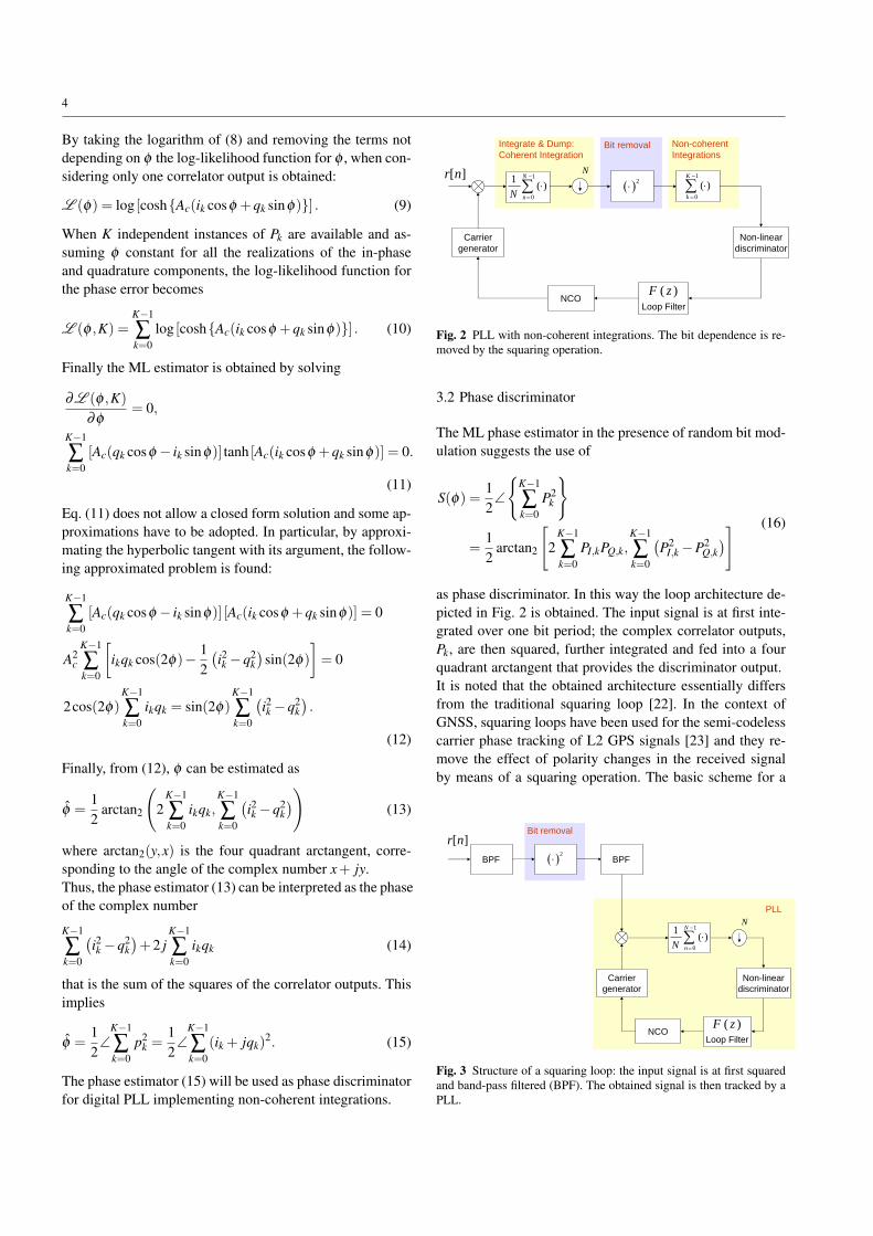
Fig. 2 PLL with non-coherent integrations. The bit dependence is re-moved by the squaring operation.

3.2 Phase discriminator

The ML phase estimator in the presence of random bit mod-ulation suggests the use of

S(φ) =12∠

{K−1

∑k=0

P2k

}

=12

arctan2

[2

K−1

∑k=0

PI,kPQ,k,K−1

∑k=0

(P2

I,k −P2Q,k)] (16)

as phase discriminator. In this way the loop architecture de-picted in Fig. 2 is obtained. The input signal is at first inte-grated over one bit period; the complex correlator outputs,Pk, are then squared, further integrated and fed into a fourquadrant arctangent that provides the discriminator output.It is noted that the obtained architecture essentially differsfrom the traditional squaring loop [22]. In the context ofGNSS, squaring loops have been used for the semi-codelesscarrier phase tracking of L2 GPS signals [23] and they re-move the effect of polarity changes in the received signalby means of a squaring operation. The basic scheme for a

( )2⋅

[ ]r nBit removal

BPF

Non-linear discriminator

( )F zLoop Filter

NCO

Carrier generator

N1

0

1 ( )N

nN

−

=

⋅∑

PLL

BPF

Fig. 3 Structure of a squaring loop: the input signal is at first squaredand band-pass filtered (BPF). The obtained signal is then tracked by aPLL.

5

squaring loop is reported in Fig. 3: in this case the squar-ing is performed outside the PLL causing the amplificationof the noise components. Moreover, the output frequency istwice the carrier frequency causing a half-wavelength am-biguity [23]. These two problems are overcome by the pro-posed non-coherent scheme. The original frequency infor-mation is preserved and the noise amplification is reducedby the integrate and dump filter preceding the squaring block.It is noted that the non-coherent integration block in Fig. 2acts as a moving average filter. In this way, the input of thefour quadrant arctangent is a correlated process which de-pends on the last K complex correlator outputs. Thus, thediscriminator (16) introduces memory into the loop, insert-ing new zeros and poles into the loop transfer function. Thiseffect will be better analyzed in Section 5. The memory in-troduced by the discriminator can be removed by adding adecimator after the non-coherent integration block, furtherreducing the update interval of the loop and increasing thelatency of the phase estimation. For this reason only thecase of discriminator with memory is considered hereinafter.Moreover this structure allows the design of more generaldiscriminators as discussed in Section 8.

3.3 Code discriminator

Code tracking can be interpreted as an iterative process thattends to maximize the cost function defined by the corre-lation between the input signal and a signal replica locallygenerated. The maximization is performed by adjusting thecode delay between the input signal, r[n], and its local replica.Moreover code tracking can be thought of as a gradient as-cent algorithm since the maximization is performed by fol-lowing the direction pointed by the discriminator output,that is, in some sense, an approximation or a modificationof the derivative of the cost function, i.e. the correlation. Inthis respect a code tracking loop can be designed by oppor-tunely modifying the cost function or suitably changing thediscriminator structure. For example the traditional normal-ized non-coherent early minus late envelope [17]:

S(τ) =(

1− ds

2

)|Ek|− |Lk||Ek|+ |Lk|

(17)

can be modified as follows

S(τ) =(

1− ds

2

)√∑

K−1k=0 |Ek|2 −

√∑

K−1k=0 |Lk|2√

∑K−1k=0 |Ek|2 +

√∑

K−1k=0 |Lk|2

(18)

that is, by introducing non-coherent integrations after thecorrelator outputs. In Eq.s (17) and (18) Ek and Lk denotethe kth complex Early and Late correlator outputs [16, 17]obtained by correlating the input signal with an anticipatedand delayed version of the local code, respectively.

Non-linear discriminator

( )F zLoop Filter

NCO

Carrier generator

1

0

1 ( )N

nN

−

=

⋅∑[ ]r n

Integrate & Dump: Coherent Integration

N

… …

Bit combinations max

Bit estimation & further Coherent Integration

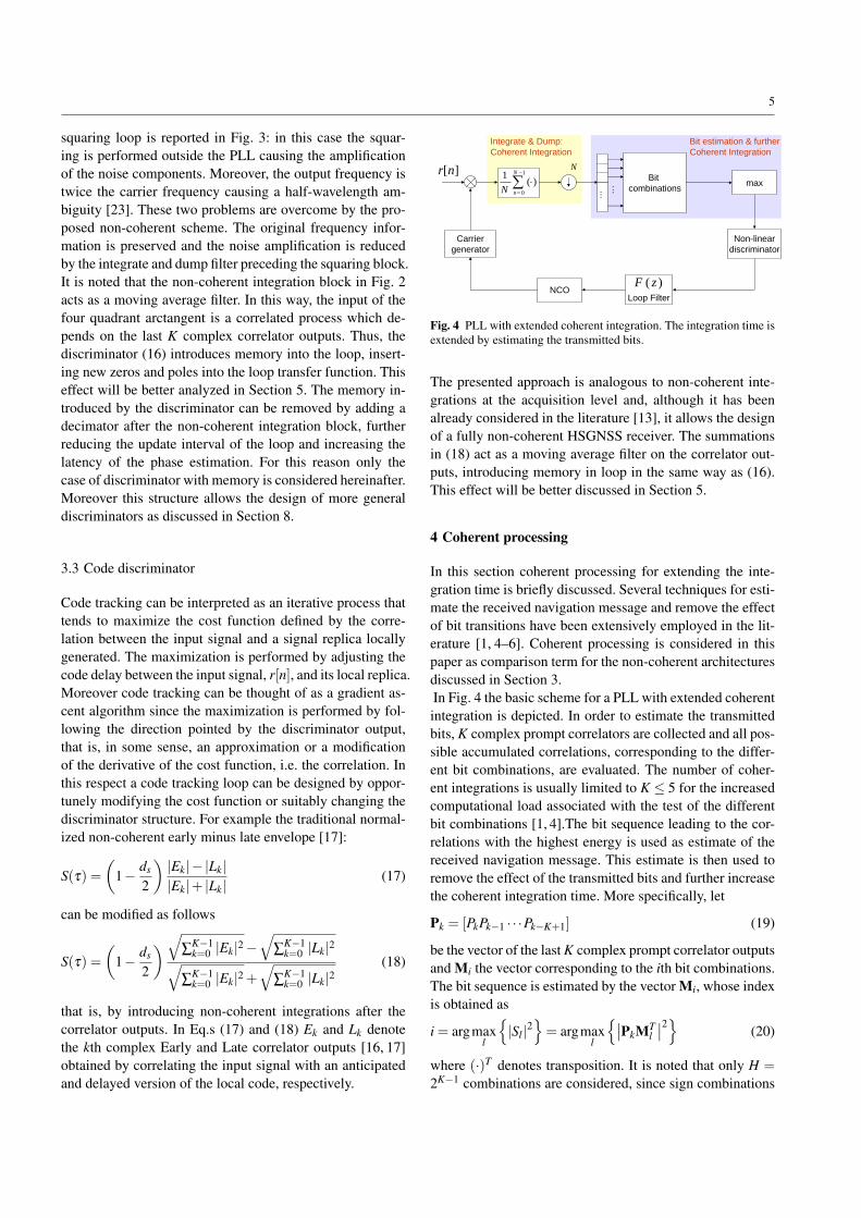
Fig. 4 PLL with extended coherent integration. The integration time isextended by estimating the transmitted bits.

The presented approach is analogous to non-coherent inte-grations at the acquisition level and, although it has beenalready considered in the literature [13], it allows the designof a fully non-coherent HSGNSS receiver. The summationsin (18) act as a moving average filter on the correlator out-puts, introducing memory in loop in the same way as (16).This effect will be better discussed in Section 5.

4 Coherent processing

In this section coherent processing for extending the inte-gration time is briefly discussed. Several techniques for esti-mate the received navigation message and remove the effectof bit transitions have been extensively employed in the lit-erature [1, 4–6]. Coherent processing is considered in thispaper as comparison term for the non-coherent architecturesdiscussed in Section 3.In Fig. 4 the basic scheme for a PLL with extended coherentintegration is depicted. In order to estimate the transmittedbits, K complex prompt correlators are collected and all pos-sible accumulated correlations, corresponding to the differ-ent bit combinations, are evaluated. The number of coher-ent integrations is usually limited to K ≤ 5 for the increasedcomputational load associated with the test of the differentbit combinations [1, 4].The bit sequence leading to the cor-relations with the highest energy is used as estimate of thereceived navigation message. This estimate is then used toremove the effect of the transmitted bits and further increasethe coherent integration time. More specifically, let

Pk = [PkPk−1 · · ·Pk−K+1] (19)

be the vector of the last K complex prompt correlator outputsand Mi the vector corresponding to the ith bit combinations.The bit sequence is estimated by the vector Mi, whose indexis obtained as

i = argmaxl

{|Sl |2

}= argmax

l

{∣∣PkMTl

∣∣2} (20)

where (·)T denotes transposition. It is noted that only H =2K−1 combinations are considered, since sign combinations

6

DiscriminatorModel

( )B z

Linearized discriminator

( )F zLoop Filter

NCO

Equivalent Noise

[ ]dN k

[ ] kφ

[ ] kφ

-

[ ] kφ

[ ] kφ

Fig. 5 Linear model for a tracking loop with discriminator with mem-ory. In traditional tracking loop the discriminator is substituted by anamplifier with constant gain.

differing only for the absolute sign would lead to the sameenergy. Mi is then used to extend the integration time pro-ducing the accumulated correlator outputs that will be fedinto traditional discriminators. For example, the phase dis-criminator is given by

S(φ) = arctan

(ℜ{

PkMTi}

ℑ{

PkMTi

}) . (21)

It is noted that also extended coherent integrations can in-troduce memory at the discriminator level. This depends onthe way the vector Pk is updated. In fact, if the vector Pk+1is obtained from Pk by substituting the oldest prompt cor-relator output with Pk+1, the correlator output evaluated atinstant k+1, then a moving average effect is introduced andthe analysis presented in Section 5 also applies to this kindof loops.

5 Linear model and filter design

In this section the linear model for discriminators with mem-ory, such as the ones described in Sections 3 and 4 is derived.Moreover the linear model is used to evaluate the transferfunction of the loop and define the design criteria for theloop filter.The linear model for a tracking loop and its transfer func-

tion can be obtained by substituting the loop discriminatorwith its linear approximation. In Fig. 5 the linear model fora generic tracking loop is depicted. In this case the loop isrepresented with respect to the quantity to be tracked. In thefollowing the PLL case is considered although the reportedresults are general and apply to the other loops consideredin the paper. In Fig. 5

– φ [k] is the average phase at the correlator output that theloop is trying to track;

– φ [k] is the phase estimated from the loop;– ˙

φ [k] is the phase rate at input of the NCO;– φ [k] is the phase estimated by the discriminator;

– Nd [k] is a white random process accounting for the noiseat the input of the loop and the distortions introduced bythe non-linearities in the discriminator.

In traditional tracking loops, the discriminator is approxi-mated by a constant gain. However in the architecture de-scribed in the previous sections, the discriminator employsthe last K complex correlations, Pk, to evaluate an estimateof the phase error φ . Thus, this kind of discriminators intro-duces memory into the system and a more appropriate linearapproximation is a Finite Impulse Response (FIR) filter:

B(z) =K−1

∑i=0

aizK−1 (22)

where

ai =∂

∂φ [i]E[S]

∣∣∣∣φ [i]=0

. (23)

A FIR model is adopted, since only a finite number of corre-lator outputs is used for the evaluation of the discriminatoroutput. It is noted that, for K = 1, the linear model (22) be-comes a constant gain corresponding to the model usuallyadopted for tracking loops.It can be shown that for the normalized discriminators con-sidered in the paper

ai =1K

for 0 ≤ i < K. (24)

The coefficients of the linear expansion (22) assume the con-stant value 1/K. This is due to the fact that the discrimina-tor equally weights the different complex correlations Pk. Inthis respect, more complex discriminators, accounting forthe fact that older correlations should impact less the esti-mation of the current phase, can be designed by introduc-ing unequal weights as discussed in Section 8. From (24) itfollows that the linear approximation for the considered dis-criminators is given by a moving average filter with transferfunction

B(z) =1K

K−1

∑i=0

z−i. (25)

In the absence of noise, the discriminator output can be ap-proximated as

φ [k] =(φ [k]− φ [k]

)∗b[k] (26)

where b[k] is the inverse Z-transform of B(z).The closed loop transfer function is defined as [15]:

H(z) =φ(z)φz

(27)

where φ(z) and φ(z) are the Z-transforms of the input andestimated phases φ [k] and φ [k], respectively.

7

-1 -0.5 0 0.5 1-1

-0.5

0

0.5

1

Real Part

Imag

inar

y P

art

K = 1, Bn = 5 Hz

-1 -0.5 0 0.5 1-1

-0.5

0

0.5

1

Real Part

Imag

inar

y P

art

K = 2, Bn = 5.4 Hz

-1 -0.5 0 0.5 1-1

-0.5

0

0.5

1

Real Part

Imag

inar

y P

art

K = 4, Bn = 6.8Hz

-1 -0.5 0 0.5 1-1

-0.5

0

0.5

1

Real Part

Imag

inar

y P

art

K = 8, Bn = 18.25 Hz

Fig. 6 Zeros and poles of the loop transfer function for different values of K. The loop filter is a 2nd order filter and the coefficients are keptconstant for all cases. The coefficients were designed to provide a 5 Hz bandwidth for K = 1.

The single-sided loop noise bandwidth Bn for the closedloop is defined as [15]

Bn =12

∫ 1/2T

−1/2T

∣∣H (e j2π f T )∣∣2 d f

=12

12π jT

∮H(z)H

(z−1)z−1dz

(28)

and is one of the main parameters for the loop design: nar-row bandwidths harden the tracking loop against thermalnoise at the expenses of reduced tracking dynamic capabili-ties.H(z) and Bn can be evaluated once the loop filter and theNCO models are defined. More specifically, integrator-basedloop filters are characterized by the following transfer func-tion:

F(z) =1T

L−1

∑i=0

Ki1

(1− z−1)i =1T

L−1

∑i=0

Ki

[z

z−1

]i

. (29)

In this case the loop filter is constrained to be a linear com-bination of several integrators of different order. L definesthe order of the loop. The use of integrator-based filters al-lows the loop to provide unbiased phase estimates for inputphases varying according to polynomial models of degree L.In a rate-only feedback NCO, the phase estimate is updatedaccording to the following equation [15]

φ [k +1] = φ [k]+12

(˙φ [k +1]T + ˙

φ [k]T)

. (30)

Using Eq.s (26), (29) and (30) the loop transfer function canbe finally evaluated as

H(z) =12 (z+1)T B(z)F(z)

z(z−1)+ 12 (z+1)T B(z)F(z)

=DK(z)− zK(z−1)L

DK(z)

(31)

8

where

DK(z) = zK(z−1)L +1

2K(z+1)

K−1

∑j=0

z jL−1

∑i=0

Kizi (z−1)L−i−1 .

(32)

It is noted that (31) has the same structure as the transferfunctions of traditional tracking loops with rate-only feed-back NCO. Moreover, (31) can be used to verify that track-ing loops with memory discriminators provide unbiased phaseestimates for input phases varying according to a polynomialmodel of degree L.The presence of the discriminator with memory increasesthe order of the system by introducing new poles and zeros.In particular K − 1 zeros are introduced, corresponding tothe solutions of 1− zK = 0 different from z = 1. The zero,z = 1, is only apparent and is canceled out by the corre-sponding pole. In Fig. 6 the poles of (31) are plotted fordifferent K, for a second order loop filter. The coefficientsof the loop filter, K0 = 0.2166 and K1 = 0.0265, are keptconstant for all cases. Those coefficients were designed toprovide a 5 Hz bandwidth for K = 1. As K increases newpoles appear and the original poles due to the loop filter,are pushed towards the unit circle. This effect reduces thestability margin of the system and increases the equivalentbandwidth. For this reason specific filter design techniques,accounting for the additional poles, have to be adopted.

5.1 Controlled-Root Formulation

In order to properly design the loop filter a controlled-rootformulation [15] has been adopted. It is noted that other ap-proaches, based on optimality criteria can be adopted [24].These approaches are not considered here and left as futurework. The controlled-root formulation was originally pro-posed by [15] for memoryless discriminators and has beenextended here in order to account for the extra poles intro-duced by a discriminator with memory. More specifically,in the controlled-root formulation the poles of the loop fil-ter are constrained to lie on specific positions depending ondesign parameters, such as the decay-rate and the dampingfactor. In this way, the poles are positioned in order to en-sure a stable loop and the design parameters are adjusted inorder to meet the bandwidth requirements. When the case ofmemory discriminators is considered it is not possible to fixthe positions of all the loop poles since only L free parame-ters, the L integrator gains, are available. This L parametersallow one to fix only L poles. Thus the algorithm derivingfrom the controlled-root formulation has been modified asreported in Fig. 7.

At first L poles are fixed according to some initial valuesof the design parameters. By substituting the values of theseL poles into (32), a system of L equations in L unknowns

Fix the position of

L poles

Determine the position of the remaining poles exploiting

the constraints imposed by the transfer function structure

Find the integrator gains

Determine the loop

bandwidth

Adjust the pole positions until the right bandwidth

is obtained

Fig. 7 Iterative algorithm for filter design according to the root-controlled formulation.

is found. By solving this system the integrator gains are ob-tained. The integrator gains define the transfer function ofthe system, from which the loop bandwidth can be evalu-ated. The design parameters are iteratively adjusted until therequired bandwidth is obtained.It has been noted that the additional poles introduced by thediscriminator are always placed closer to the origin of the Z-plane than the poles placed according to design parameters.In this way, stable loops with the desired bandwidth wereobtained.

6 Phase tracking jitter

In this section, coherent and non-coherent integration strate-gies are compared in terms of phase tracking jitter. Phasetracking jitter allows one to quantify the impact of thermalnoise on the PLL and it is defined as [16]:

σ j =σs

Gd

√2BnT (33)

where σs is the standard deviation of the discriminator out-put, Bn is the loop equivalent bandwidth and Gd is the dis-criminator gain defined as

Gd =dE [S (φ)]

dφ

∣∣∣∣φ=0

. (34)

Theoretical and Monte Carlo simulations are used to evalu-ate the phase tracking jitter when coherent and non-coherentintegrations are used at the PLL level. The simulation pa-rameters are reported in Table 1. In general, the tracking jit-ter measures the Root Mean Square (RMS) phase error ofthe loop and can be expressed as [23, 25]

σ j =

√[C

N0BnSL

]−1

(35)

9

Table 1 Simulation parameters.

Parameter ValueSampling Frequency fs = 8.184 MHzFront-end bandwidth BIF = fs/2 = 4.092 MHz

Integration Time T = 20 msSimulation points Np = 1e5

where SL is the squaring loss. Eq. (35) can be interpretedas follows: if a PLL were a perfectly linear system, then thetracking jitter would be a measure of the Signal-to-NoiseRatio (SNR) at the output of the loop. More specifically, thetracking jitter would only depend on the product of the inputC/N0 and the inverse of the loop bandwidth. Since a PLL isin general a non-linear device, performance is degraded bythe additional noise introduced by the non-linearities. Thisimpact is measured by the squaring loss SL.It has been shown [23] that, when the bandwidth of the in-tegrate and dump filter in the PLL is wide enough not tointroduce signal distortion, the squaring loss can be approx-imated by

SL ≈1

1+ 12C/N0T

(36)

leading to the following expression for the tracking jitter:

σ j =

√Bn

C/N0

(1+

12C/N0T

). (37)

It is noted that (37), is a general formula corresponding tothe usual tracking jitter for Costas loop [17]. Moreover, (37)does not depend on the number of non-coherent integrations,K, but only on the input C/N0, the loop bandwidth and thecoherent integration time T . It is noted that, as demonstratedin Section 7, when K > 1 non-coherent integrations are em-ployed, a PLL with lower equivalent bandwidth Bn can beused. Moreover, by increasing the integration time less noisymeasurements are expected.Formula (37) has been verified by Monte Carlo simulationsand, in Fig. 8, some simulation results are summarized. Morespecifically, the case of a constant product

KBnT = 0.2

has been considered and three different values of K investi-gated. The tracking jitter obtained by simulations matchesthe theoretical value, supporting the validity of (37). Thevertical trend in the simulated curves indicate that the loophas lost lock.In Fig. 9 coherent and non-coherent integrations are com-

pared in terms of tracking jitter. It is noted that the trackingjitter for a Costa loop can be lower bounded by

σ j ≤

√Bn

C/N0

(1+

12KC/N0T

)(38)

18 20 22 24 26 28 30 32 340

0.05

0.1

0.15

0.2

0.25

0.3

0.35

0.4KBnT = 0.2, T = 20 ms

C/N0 (dB-Hz)

Jitte

r (ra

d)

SimulatedTheoretical

K = 1

K = 3

K = 5

Fig. 8 Comparison between theoretical and simulated phase trackingjitter for constant KBnT and for different numbers of non-coherent in-tegrations. The vertical trends indicate that the simulated loop has lostlock.

18 20 22 24 26 28 30 32 340

0.05

0.1

0.15

0.2

0.25

0.3KBnT = 0.2, T = 20 ms

C/N0 (dB-Hz)

Jitte

r (ra

d)

Theoretical lower boundCoherent CombiningNon-coherent Combining

K = 7

K = 5

K = 3

Fig. 9 Comparison between coherent and non-coherent integrationsin terms of phase tracking jitter. The vertical trends indicate that thesimulated loop has lost lock.

which corresponds to the case of an ideal loop able to co-herently integrate, without estimating the transmitted bits,up to KT , the total integration time. This lower bound isplotted in Fig. 9 as reference. As expected, coherent integra-tion slightly outperforms non-coherent integration in termsof tracking jitter. This is however achieved at the expensesof an increased computational complexity. In Fig. 9 only theimpact of thermal noise has been considered, since both the-oretical model and simulations do not consider the effect ofdynamics and phase noise introduced by the oscillator andthe other electronic devices present the receiver chain. This

10

National Instruments PXI-5661

Customized GSNRxTM

Software Receiver

Roof antenna

Variable Attenuator

Ref. GPS Unit Timing Source PC

Reference GPS signalData storage

Fig. 10 Experimental setup: the GPS signal has been collected by us-ing two different front-ends. One of the recovered signals has beenprogressively attenuated in order to obtain different C/N0 conditions.

aspect will be better investigated in Section 7, where someresults obtained with real data are presented.

7 Experimental results

In order to test the proposed discriminators with non-coherentintegrations and verify the correct design of the loop filtersa customized version of the University of Calgary’s GNSSSoftware Navigation Receiver (GSNRxT M) [14] has beendeveloped and tested by means of real data. GSNRxT M isa flexible and reconfigurable tool, developed in C++. In thisrespect, the discriminators with extended coherent and non-coherent integrations have been implemented and integratedin the existing version of the GSNRxT M . The loop filtershave been also modified according to the methodology de-scribed in Section 5.1.Live GPS data have been collected according to the exper-imental setup described in Fig. 10. The received signal hasbeen progressively attenuated in order to obtain a decreasingC/N0. Only the case of a static receiver is considered in thepaper and thus, the only dynamics present in the receivedsignal are those caused by the satellite motion and the clockdrift. It is noted that the case of a static receiver is usuallyadopted for testing long integration based algorithms [4, 5]and that external sensors are generally used to compensatethe effect of the user motion under high dynamic conditions.The GPS signal has been collected using a NI PXI-5661 sig-nal analyzer [26], using the specifications reported in Table2. After a minute without attenuation the signal was pro-gressively attenuated with a step of 1 dB each 30 s. It isnoted that the decrease in C/N0 is not directly proportionalto the provided attenuation since both signal and noise com-ponents were attenuated at the same time. More specifically,the decrease in C/N0 is caused by both the signal attenua-tion and the additional noise introduced by the attenuator.In the following the signal from PRN 02 is analyzed. PRN

02 was selected since it was the one characterized by the

Table 2 Characteristics of the collected GPS signals.

Parameters ValueSampling frequency fs = 10 MHz

intermediate frequency fIF = 3.42 MHzSampling Real

Fig. 11 C/N0 and carrier Doppler estimated for the PRN 02 as a func-tion of the number of non-coherent integrations. Bn = 5 Hz.

Table 3 Loss of lock conditions measured for the PRN 02, PLL band-width Bn = 5 Hz

K Integration Type Time Estimated C/N0

1 9.4 min 14 dB-Hz2 Non-coherent 9.2 min 14.5 dB-Hz2 Coherent 9.2 min 14.5 dB-Hz4 Non-coherent 9.8 min 12 dB-Hz4 Coherent 9 min 15 dB-Hz

lowest C/N0. Similar results were obtained by processingthe signals transmitted from the other satellites although highervalues of C/N0 were obtained. In Fig.s 11 and 12 the caseof a PLL with a 5 Hz bandwidth is considered. More specif-ically, the C/N0 and carried Doppler estimations are shownas a function of time. In Fig. 11 the case of non-coherent in-tegration is analyzed whereas Fig. 12 deals with the case ofcoherent integrations. For K = 1, the system is able to trackthe signal for a C/N0 as low as 14 dB-Hz. When increasingthe number of non-coherent integrations the signal lock islost at around 14.5 dB-Hz for K = 2 and around 12 dB-Hzfor K = 4. On the contrary, when using coherent integra-tion the lock is lost for increasing C/N0 when the numberof integrations is increased. This could indicate that, for lowC/N0, the process of bit estimation becomes unreliable andthe PLL tends to be driven only by noise, causing loss oflock. The results for Bn = 5 Hz are summarized in Table 3.

11

Fig. 12 C/N0 and carrier Doppler estimated for the PRN 02 as a func-tion of the number of coherent integrations. Bn = 5 Hz.

Fig. 13 C/N0 and carrier Doppler estimated for the PRN 02 as a func-tion of the number of non-coherent integrations. Bn = 2 Hz.

In order to further test the advantages brought by long in-tegration, the collected data has been processed by using aPLL bandwidth as narrow as 2 Hz. With such a narrow band-width it was not possible, for K = 1, to obtain a loop able tosuccessfully track the signal. When using non-coherent inte-grations the receiver was able to obtain a stable lock and thesignal was successfully tracked for C/N0 close to 10 dB-Hz,as demonstrated in Fig. 13. The case of coherent integrationsis shown in Fig. 14: although the receiver was able to obtaina stable lock, the signal is lost only after about 8.5 minutes.It is noted that long integrations reduce the variance of theestimated carrier Doppler. This fact was already observed

Fig. 14 C/N0 and carrier Doppler estimated for the PRN 02 as a func-tion of the number of coherent integrations. Bn = 2 Hz.

7.8 7.9 8 8.1 8.2 8.3 8.4

-370

-365

-360

-355

-350

-345

Time (min)

Car

rier D

oppl

er (

Hz)

PRN 02, Bn = 5 Hz

K = 1K = 2K = 4

Fig. 15 Estimated carrier Doppler for the PRN02. The use of non-coherent integrations reduces the variance of the estimated quantities.

by [7] for long coherent integrations and holds true alsofor the case of non-coherent integrations as demonstratedby Fig. 15. In Fig. 15 the carrier Doppler for PRN 02 isshown over a short period of time, better highlighting theimpact of increasing non-coherent integrations. The impactof the number of integrations on the observation noise hasbeen further studied by using results from PRN 20. PRN 20was chosen since it was characterized by an estimated C/N0decreasing almost linearly with time. This fact allowed toeasily estimate the variance of the carrier Doppler observa-tion as a function of the C/N0. In Fig. 16 the evolution ofthe C/N0 for PRN 20 is reported as function of time. In Fig.17 the standard deviation of the carrier phase observation is

12

5 5.5 6 6.5 7 7.5 8 8.5

24

26

28

30

32

34

36

Time (min)

C/N

0 (dB

-Hz)

PRN 20

Fig. 16 C/N0 evolution for the PRN 20.

25 26 27 28 29 30 31 32 33 34 35 360

0.05

0.1

0.15

0.2

0.25

0.3

C/N0 (dB-Hz)

Car

rier D

oppl

er E

rror

- S

td d

evia

tion

(Hz)

PRN 20 - Bn = 2 Hz

Non-coherentCoherent

K = 1

K = 2

K = 4

Fig. 17 Standard deviation on the carrier Doppler observations as afunction of the C/N0 and the number of integrations.

reported as a function of the measured C/N0. A PLL band-width of 2 Hz was considered and, in this case the initialC/N0 was high enough to allow the PLL to have a stable lockalso for K = 1. As expected the standard deviation of themeasured carrier Doppler decreases as the C/N0 increases.Moreover, lower standard deviations are obtained for highervalues of K, the number of integrations. It is noted that co-herent integrations slightly outperform their non-coherentcounterpart. However, the difference is marginal and it isobtained at the expense of an increased computational load.

8 Future work: generalized memory discriminators

In Section 3 a non-coherent phase discriminator was ob-tained as (16)

S(φ) =12∠

K−1

∑k=0

P2k

where the inner summation was interpreted as a moving av-erage filter. A generalization of such a discriminator can beeasily obtained by substituting the moving average filter bya more general filter:

S(φ) =12∠

+∞

∑k=0

hkP2k (39)

where the coefficients {hk}+∞

k=0 define the impulse responseof the filter

h[n] =+∞

∑k=0

hkδ [n− k]. (40)

δ [n] denotes the Kronecker delta. The introduction of a gen-eral filter h[n] instead of the moving average window is jus-tified by the fact that the oldest samples, Pk, should impactless the current phase estimation than the most recent ones.A simple choice for h[n] is represented by the exponentialfilter defined by

h[n] = (1−α)+∞

∑k=0

αkδ [n− k] with 0 < α < 1. (41)

By adopting (41) the square correlator outputs are progres-sively de-weighted according to the forgetting factor α . Thiskind of discriminator can be easily implemented using a re-cursive formula and it is currently under investigation.

9 Conclusions

In this paper, a non-coherent architecture for GNSS trackingloops has been proposed and analyzed. More specifically, aphase detector, employing several correlator outputs and im-mune to bit transitions has been designed according to theMaximum Likelihood principle. A fully non-coherent re-ceiver architecture has been obtained by adopting a DLL dis-criminator with non-coherent integrations. New digital loopfilters have been designed, by extending the root-controlledfilter formulation to the case of discriminators with mem-ory. This has led to a fully operational GNSS receiver capa-ble of long integration times. The proposed algorithms havebeen compared with existing methodologies for coherentlyextending the integration time, resulting in an effective al-ternative to bit-estimation based techniques.

13

10 Acknowledgments

The authors would like to kindly acknowledge and thankDefence Research and Development Canada (DRDC) forfunding this work.

References

1. M. Petovello, C. ODriscoll, and G. Lachapelle, “Weak signal car-rier tracking using extended coherent integration with an ultra-tight GNSS/IMU receiver,” in Proc. of the European NavigationConference, Toulouse, France, Apr. 2008.

2. S. T. Lowe, “Voltage Signal-to-Noise ratio (SNR) nonlinearity re-sulting from incoherent summations,” The Telecommunicationsand Mission Operations Progress Report, TMO PR 42-137, Tech.Rep., May 1999.

3. C. Strassle, D. Megnet, H. Mathis, and C. Burgi, “The squaring-loss paradox,” in Proc. of ION/GNSS, Fort Worth, TX, Sept. 2007,pp. 2715 – 2722.

4. A. Soloviev, F. van Graas, and S. Gunawardena, “Implementationof Deeply Integrated GPS/Low-Cost IMU for Reacquisition andTracking of Low CNR GPS Signals,” in Proc. of ION NationalTechnical Meeting NTM, San Diego, CA, Jan. 2004, pp. 923 –935.

5. A. Soloviev, S. Gunawardena, and F. van Graas, “Deeply In-tegrated GPS/Low-Cost IMU for Low CNR Signal Processing:Flight Test Results and Real Time Implementation,” in Proc. ofION/GNSS, Long Beach, CA, Sept. 2004, pp. 1598 – 1608.

6. M. L. Psiaki and H. Jung, “Extended kalman filter methods fortracking weak GPS signals,” in Proc. of ION/GPS, Portland, OR,Sept. 2002, pp. 2539 – 2553.

7. P. L. Kazemi and C. ODriscoll, “Comparison of Assisted andStand-Alone Methods for Increasing Coherent Integration Timefor Weak GPS Signal Tracking,” in Proc. of ION/GNSS’08, Sa-vannah, GA, Sept. 2008, in press.

8. Carlos A. Pomalaza-Raez, “Analysis of an all-digital data-transition tracking loop,” IEEE Trans. Aerosp. Electron. Syst.,vol. 28, no. 4, pp. 1119 – 1127, Oct. 1991.

9. M. K. Simon and A. Tkacenko, “Noncoherent data transitiontracking loops for symbol synchronization in digital communica-tion receivers,” IEEE Trans. Commun., vol. 54, no. 5, pp. 889 –899, May 2006.

10. C. O’Driscoll, “Performance analysis of the parallel acquisitionof weak GPS signals,” Ph.D. dissertation, National University ofIreland, Cork, Jan. 2007.

11. C. J. Hegarty, “Optimal and near-optimal detector for acquisitionof the GPS L5 signal,” in Proc. of ION NTM, National TechnicalMeeting, Monterey, CA, Jan. 2006, pp. 717 – 725.

12. D. Borio, C. O’Driscoll, and G. Lachapelle, “Coherent, non-coherent and differentially coherent combining techniques for theacquisition of new composite GNSS signals,” IEEE Trans. Aerosp.Electron. Syst., May 2008, in press.

13. H. Hurskainen, E. S. Lohan, X. Hu, J. Raasakka, and J. Nurmi,“Multiple Gate Delay Tracking Structures for GNSS Signals andTheir Evaluation with Simulink, SystemC, and VHDL,” Interna-tional Journal of Navigation and Observation, p. 17, Feb. 2008.

14. M. G. Petovello and C. O’Driscoll, GSNRxT M User Manual, Po-sition, Location And Navigation (PLAN) Group, Department ofGeomatics Engineering, Schulich School of Engineering, TheUniversity of Calgary, 2500 University Drive NW Calgary, AB,Canada, T2N 1N4, Aug. 2007.

15. S. A. Stephens and J. Thomas, “Controlled-root formulation fordigital phase-locked loops,” IEEE Trans. Aerosp. Electron. Syst.,vol. 31, no. 1, pp. 78 – 95, Jan. 1995.

16. A. J. Van Dierendonck, P. Fenton, and T. Ford, “Theory and per-formance of narrow correlator spacing in a gps receiver,” NAVI-GATION: Journal of The Institute of Navigation, vol. 39, no. 3,pp. 265 – 283, Fall 1992.

17. E. D. Kaplan and C. J. Hegarty, Eds., Understanding GPS: Prin-ciples and Applications, 2nd ed. Norwood, MA, USA: ArtechHouse Publishers, 2005.

18. J. W. Betz and K. R. Kolodziejski, “Generalized theory of codetracking with early-late discriminator, part 1: Lower bound andcoherent processing,” IEEE Trans. Aerosp. Electron. Syst., Mar.2008, in press.

19. ——, “Generalized theory of code tracking with early-late dis-criminator, part 2: Noncoherent processing and numerical results,”IEEE Trans. Aerosp. Electron. Syst., Mar. 2008, in press.

20. J. W. Betz, “Effect of partial-band interference on receiver estima-tion of C/N0: Theory,” in Proc. of ION National Technical Meet-ing, Long Beach, CA, Jan. 2001, pp. 817 – 828.

21. J. W. Betz and N. R. Shnidman, “Receiver processing losses withbandlimiting and one-bit sampling,” in Proc. of ION GNSS, FortWorth, TX, Sept. 2007.

22. W. C. Lindsey and M. K. Simon, Telecommunication Systems En-gineering. Dover Publications, Aug. 1991.

23. K. T. Woo, “Optimum semi-codeless carrier phase tracking of l2,”in Proc. of ION GPS’99, Nashville, TN, Sept. 1999, pp. 289 – 305.

24. P. L. Kazemi, “Optimum Digital Filters for GNSS TrackingLoops,” in Proc. of ION/GNSS’08, Savannah, GA, Sept. 2008, inpress.

25. M. Simon and W. Lindsey, “Optimum performance of suppressedcarrier receivers with costas loop tracking,” IEEE Trans. Com-mun., vol. 25, no. 2, pp. 215 – 227, Feb. 1977.

26. 2.7 GHz RF Vector Signal Analyzer with Dig-ital Downconversion, National Instruments,http://www.ni.com/pdf/products/us/cat vectorsignalanalyzer.pdf,2006.