gnss signal tracking under weak signal or high dynamic
TRANSCRIPT

This document is downloaded from DR‑NTU (https://dr.ntu.edu.sg)Nanyang Technological University, Singapore.
GNSS signal tracking under weak signal or highdynamic environment
Yang, Rong
2017
Yang, R. (2017). GNSS signal tracking under weak signal or high dynamic environment.Doctoral thesis, Nanyang Technological University, Singapore.
http://hdl.handle.net/10356/70121
https://doi.org/10.32657/10356/70121
Downloaded on 17 Mar 2022 18:01:17 SGT

GNSS Signal Tracking under Weak
Signal or High Dynamic
Environment
Yang Rong
School of Electrical and Electronic Engineering
2016

GNSS Signal Tracking under Weak
Signal or High Dynamic
Environment
Yang Rong
School of Electrical and Electronic Engineering
A Thesis Submitted to the Nanyang Technological University in
Fulfilment of the Requirements for the Degree of Doctor of Philosophy
Supervised by
Assoc. Prof. LING Keck Voon
2016

Acknowledgments
I would like to express my gratitude to those who have inspired, encouraged, and
supported me during my Ph.D study.
Firstly, I would express my deepest gratitude to my supervisor Associate Professor
Ling Keck Voon and co-supervisor Associate Professor Poh Eng Kee for their patien-
t guidance and consistent support throughout my research work. Their profound
knowledge, solid research skills, patience, and enthusiasm have significant impacts on
my research. I am truly grateful to have the opportunity to complete this interesting
research work under the guidance of Prof Ling and Prof Poh.
Secondly, I am extremely thankful to Professor Yu Morton of Colorado State
University, who has a long-lasting influence on both my research and my personal
development. She shares her knowledge, wisdom, and experience with me on my
Ph.D study. Without her valuable guidance and kind encouragement, it would be
much more difficult for me to finish this academic journey.
Thirdly, I would like to acknowledge my former supervisor, Professor Qin Honglei
of Beihang University. I gained my interest in GNSS from a project Prof. Qin guided
me during my graduate years, and he alerted and advised me this opportunity to
come to Nanyang Technological University.
In addition, my sincere gratitude to Associate Professor Low Kay Soon in Satellite
Research Center who offered me the scholarship and allowed me to attend his group
meeting. It is a wonderful experience to have so many technical discussions with his
team in the meeting. Also, I would like to thank the staff and students in INFINITUS
and Satellite Research Center of Nanyang Technological University who have helped
me both in study and life in Singapore, including Dr Jin Tian (Beihang University),
i

Dr Cong Li (Beihang University), Dr Zhu Yunlong (Beihang University), Dr Zhao Yun
(Beihang University), Dr Chen Le (Shanghai Jiao Tong University), Dr He Xin, Dr
Wu Lin (Huazhong University of Science and Technology), Dr Li Xiang(Huazhong
University of Science and Technology), Ms Huang Jiajia, Ms Zhao Ming, Ms Sun
Meng, Ms Gao Yumeng, Mr Wang Yang, Mr Liu Yunxiang, Mr Luo Sheng, Mr
Zhang Heng, Mr Li Beibei, Mr Wang Wei, Mr Wang Guoming, Mr Hu Hao, Mr Kang
Binyin, and Mr Han Bo. Please accept my apology for missing someone out.
Furthermore, a lot of ’Thank You’ should be said to my friends, who have given
me support and encouragement whenever I needed. The past few years with you
have been greatly enjoyable and colorful. They are: Ms Zhou Chi, Ms Zou Yulan,
Ms Li Xinyan, Ms Wu Dan, Ms Yu Mengting, Ms Cui Jingjing, Mr Zhou Dexiang,
Mr Cheng Tengpeng, Mr Yin Le, Mr Zhang Liangqi, Ms Li Junting, Ms Liu Li, Mr
Fang Zhejun, Ms Xiong Siyang, Ms Li Ping, Ms Qi Wenliang, Ms Yang Liwei, Mr Xu
Dongyang, Mr Zhu Yanqing, and Mr Wang Yiran.
Most of all, I am grateful to my parents and my grandma, who always support
me with their best wishes in my life. Their strong will and optimism encourage me to
pursue my dream in academic area. I would not be able to complete my Ph.D degree
without their support.
I dedicate this dissertation to the memory of my dearest grandpa, who provided me
his unparalleled love throughout his life. I learnt how to be a kind and responsible
person from him. I am grateful for his love and kindness forever. I will always
remember him in my heart.
ii

Contents
Summary vii
List of tables x
List of figures xv
List of abbreviations xvi
List of symbols xviii
1 Introduction 1
1.1 Motivation and Objectives . . . . . . . . . . . . . . . . . . . . . . . . 2
1.2 Thesis Contributions . . . . . . . . . . . . . . . . . . . . . . . . . . . 4
1.2.1 State space design framework for carrier tracking loop: . . . . 4
1.2.2 Analytical equations for tracking error variance and dynamic
stress error: . . . . . . . . . . . . . . . . . . . . . . . . . . . . 5
1.2.3 Optimization of tracking loop parameters: . . . . . . . . . . . 5
1.2.4 Adaptive phase and frequency tracking schemes: . . . . . . . . 6
1.3 Thesis Outline . . . . . . . . . . . . . . . . . . . . . . . . . . . . . . . 6
2 Review of GNSS signals and tracking technologies 1 9
2.1 Introduction . . . . . . . . . . . . . . . . . . . . . . . . . . . . . . . . 9
1Part of the materials in Chapter 2 are taken from “R. Yang, KV Ling, and EK Poh, Optimalcombination of coherent and non-coherent acquisition of weak GNSS signals, Pacific PNT, Honolulu,Hawaii, April 2015” and “R. Yang, KV Ling, and EK Poh, NCO Models for Tracking Loop Designin GNSS Software Receiver, IEEE/ION PLANS, Monterey, California, May 2014”
iii
2.2 GNSS signal background . . . . . . . . . . . . . . . . . . . . . . . . . 9
2.3 Baseband Processing in GNSS Receiver . . . . . . . . . . . . . . . . . 11
2.3.1 Acquisition . . . . . . . . . . . . . . . . . . . . . . . . . . . . 11
2.3.2 Tracking . . . . . . . . . . . . . . . . . . . . . . . . . . . . . . 16
2.4 Receiver Tracking Technologies . . . . . . . . . . . . . . . . . . . . . 24
2.4.1 Scalar Tracking . . . . . . . . . . . . . . . . . . . . . . . . . . 24
2.4.2 Vector Tracking . . . . . . . . . . . . . . . . . . . . . . . . . . 28
2.4.3 Open Loop Tracking . . . . . . . . . . . . . . . . . . . . . . . 29
2.5 General State Space Design Process . . . . . . . . . . . . . . . . . . . 31
3 State feedback/state estimator design for phase tracking loop2 34
3.1 System Model . . . . . . . . . . . . . . . . . . . . . . . . . . . . . . . 34
3.1.1 State model . . . . . . . . . . . . . . . . . . . . . . . . . . . . 35
3.1.2 Measurement model . . . . . . . . . . . . . . . . . . . . . . . 37
3.2 State Space Design For Phase Tracking Loop . . . . . . . . . . . . . . 38
3.3 B, K, and L Matrices Design Considerations . . . . . . . . . . . . . . 40
3.3.1 B and K design . . . . . . . . . . . . . . . . . . . . . . . . . . 40
3.3.2 Estimator Gain Matrix L . . . . . . . . . . . . . . . . . . . . 43
3.4 Closed Form Performance Indicators and Performance Analysis . . . 52
3.4.1 Tracking Performance Indicators . . . . . . . . . . . . . . . . 52
3.4.2 Performance Analysis . . . . . . . . . . . . . . . . . . . . . . . 54
3.5 Optimization: Minimum Average Phase Tracking Error Variance Criteria 58
3.6 Adaptive Phase Tracking Process . . . . . . . . . . . . . . . . . . . . 66
4 State feedback/state estimator design for frequency tracking loop3 69
2Chapter 3 is the phase tracking loop part of our papers “R. Yang, KV Ling, EK Poh, andY.Morton, Generalized GNSS Signal Carrier Tracking: Part I: Modelling and Analysis, accepted byIEEE Transactions on Aerospace and Electronic Systems, January 2017. ” and “R. Yang, Y.Morton,KV Ling, and EK Poh, Generalized GNSS Signal Carrier Tracking: Part II: Optimization andImplementation, accepted by IEEE Transactions on Aerospace and Electronic Systems, January2017.”
3Chapter 4 is the frequency tracking loop part of our papers “R. Yang, KV Ling, EK Poh, andY.Morton, Generalized GNSS Signal Carrier Tracking: Part I: Modelling and Analysis, accepted byIEEE Transactions on Aerospace and Electronic Systems, January 2017. ” and “R. Yang, Y.Morton,KV Ling, and EK Poh, Generalized GNSS Signal Carrier Tracking: Part II: Optimization and
iv

4.1 Signal Model . . . . . . . . . . . . . . . . . . . . . . . . . . . . . . . 70
4.1.1 State model . . . . . . . . . . . . . . . . . . . . . . . . . . . . 70
4.1.2 Measurement model . . . . . . . . . . . . . . . . . . . . . . . 71
4.2 Generalized Frequency Tracking Loop Design . . . . . . . . . . . . . 72
4.3 Estimator Gain Matrix Design . . . . . . . . . . . . . . . . . . . . . . 73
4.4 Performance Analysis . . . . . . . . . . . . . . . . . . . . . . . . . . . 76
4.4.1 Estimation error variance . . . . . . . . . . . . . . . . . . . . 76
4.4.2 Dynamic stress steady state error . . . . . . . . . . . . . . . . 77
4.4.3 The 3-sigma rule . . . . . . . . . . . . . . . . . . . . . . . . . 78
4.5 Optimization: Minimum Average Frequency Tracking Error Variance
Criteria . . . . . . . . . . . . . . . . . . . . . . . . . . . . . . . . . . 78
4.5.1 1-state frequency tracking loop . . . . . . . . . . . . . . . . . 79
4.5.2 2-state frequency tracking loop . . . . . . . . . . . . . . . . . 79
4.6 Adaptive Frequency Tracking Process . . . . . . . . . . . . . . . . . . 85
5 Simulation Results4 87
5.1 Verification of Theoretical Derivations . . . . . . . . . . . . . . . . . 88
5.1.1 Discriminator output . . . . . . . . . . . . . . . . . . . . . . . 88
5.1.2 Simulation verification . . . . . . . . . . . . . . . . . . . . . . 90
5.2 Simulation Results of adaptive phase/frequency tracking scheme . . . 92
5.2.1 Static weak signal scenario . . . . . . . . . . . . . . . . . . . . 93
5.2.2 dynamic weak signal scenario . . . . . . . . . . . . . . . . . . 102
6 Conclusions and Future Work 114
6.1 Conclusion . . . . . . . . . . . . . . . . . . . . . . . . . . . . . . . . . 114
6.2 Future Work . . . . . . . . . . . . . . . . . . . . . . . . . . . . . . . . 116
List of Publications 118
Implementation, accepted by IEEE Transactions on Aerospace and Electronic Systems, January2017.”
4Chapter 5 is simulation part of our paper “R. Yang, Y.Morton, KV Ling, and EK Poh, General-ized GNSS Signal Carrier Tracking: Part II: Optimization and Implementation, accepted by IEEETransactions on Aerospace and Electronic Systems, January 2017”
v

Bibliography 119
A Wiener filter transfer function derivation 130
B Frequency Measurement Derivation 135
C Frequency Tracking Error Covariance Matrix Derivation 137
D Optimal solution of 1-state frequency tracking loop 139
vi

Summary
There is a growing need to continue operating the Global Navigation Satellite Systems
(GNSS) receivers under increasingly challenging and stressful conditions, where signal
experiences deep fading, blockage, or high platform dynamics. As the most fragile
component of the GNSS receiver, the carrier tracking loop must achieve improved
tracking capability. The subject of GNSS tracking loop design has been well studied.
This thesis takes the control system design perspective, presents tracking loop design
as a state feedback/state estimator framework, sheds insight on frequency domain
analysis, derives optimal parameters for carrier tracking loop design, and proposes
adaptive tracking solutions for challenging environment.
Two generalized carrier tracking loops, namely, the generalized phase tracking
loop and the generalized frequency tracking loop, are studied using this state space
framework.
For the generalized phase tracking loop design, three approaches, i.e., proportional
integral filter (PIF), Wiener filter (WF), and Kalman filter (KF), are presented in an
unified manner from the state feedback/state estimator framework. With the state
space framework, analytical equations characterizing the carrier phase tracking loop
performance are derived. These equations relate the phase tracking error variance
and dynamic stress phase error to the filter design parameters, such as integration
time and noise equivalent bandwidth, as well as other parameters, such as thermal
noise, oscillator noise, and receiver platform dynamics. From these equations, filter
design parameters are optimized under various operating scenarios, such as weak
signal or high dynamics. More specifically, the tracking sensitivities of the generalized
phase tracking loop with these designs are obtained. Building on this analysis, an
vii

adaptive phase tracking scheme with time-varying integration time or loop bandwidth
is proposed.
A similar approach is applied to frequency tracking loop design. The PIF design is
mapped to the state space structure through the equivalent closed-loop transfer func-
tion. Traditional KF-based frequency tracking loop design assumes white Gaussian
noise. However, the frequency error measurement noise is non-white and so analyti-
cal equations for the frequency tracking error variance and dynamic stress frequency
error are derived, taking into account the non-white noise characteristic. Frequency
tracking error variance is used to evaluate the frequency tracking loop performance
under the effects of thermal noise, oscillator noise, and platform dynamics. Using
these analytical equations, optimal loop parameters are obtained, and the frequency
tracking sensitivity is characterized. Based on these theoretical analysis, an adaptive
frequency tracking scheme with loop bandwidth is proposed.
Simulation results demonstrate the effectiveness of the proposed adaptive gener-
alized carrier phase/frequency tracking architecture and verify the theoretical predic-
tion.
viii

List of Tables
1.1 Attenuation of different building material [1, 2] . . . . . . . . . . . . . 1
2.1 Loop Filter Characteristics . . . . . . . . . . . . . . . . . . . . . . . . 20
3.1 Theoretical PLL tracking sensitivities with thresholds of 15◦ (data
channel) and 30◦ (pilot channel) values for static, low, and high sig-
nal dynamics, both high and low receiver oscillator qualities, and the
optimal PIF-, WF-, and KF-based phase tracking loop designs (unit:
dB-Hz) . . . . . . . . . . . . . . . . . . . . . . . . . . . . . . . . . . . 60
3.2 Topt and BNopt parameter values for static, low, and high signal dy-
namics, both high and low receiver oscillator qualities, and PIF-, WF-,
and KF-based phase tracking loop designs . . . . . . . . . . . . . . . 63
4.1 Theoretical frequency tracking loop tracking sensitivities with thresh-
olds of 124T
(data channel) and 112T
(pilot channel) for static, low, and
high signal dynamics, both high and low receiver oscillator qualities,
and optimal frequency tracking loop designs (unit: dB-Hz) . . . . . . 83
4.2 BWopt parameter values for low and high signal dynamics, and both
high and low receiver oscillator qualities in 2-state PIF-based frequency
tracking loop design . . . . . . . . . . . . . . . . . . . . . . . . . . . . 84
5.1 Validation of analytic equations (3.64) and (3.72) in 2-state phase
tracking loop for various LOS accelerations when C/N0 = 46dB-Hz . 90
ix

5.2 Validation of analytic equations (3.64) and (3.72) in 3-state phase
tracking loop for various LOS accelerations when C/N0 = 46dB-Hz . 90
5.3 Validation of analytic equations (4.33) and (4.39) in 1-state and 2-state
frequency tracking loops for various LOS accelerations when C/N0 =
46dB-Hz . . . . . . . . . . . . . . . . . . . . . . . . . . . . . . . . . . 91
x

List of Figures
2.1 Software GNSS receiver acquisition searching area. . . . . . . . . . . 11
2.2 The architecture of coherent and non-coherent combining acquisition. 13
2.3 Coherent(N = 1) and non-coherent(M = 1) combining acquisition
result of PRN 14 satellite signal at C/N0 = 43dB-Hz (acquired). . . . 15
2.4 Coherent(N = 1) and non-coherent(M = 1) combining acquisition
result of PRN 28 satellite signal (not acquired). . . . . . . . . . . . . 15
2.5 Generic GNSS code and carrier tracking loops block diagram. . . . . 16
2.6 Generic analog phase lock loop block diagram. . . . . . . . . . . . . . 17
2.7 Block diagrams of: (a) first-, (b) second-, and (c) third-order analog
PLLs. . . . . . . . . . . . . . . . . . . . . . . . . . . . . . . . . . . . 19
2.8 Block diagrams of discrete loop filters in (a) first-, (b) second-, and (c)
third-order PLLs. . . . . . . . . . . . . . . . . . . . . . . . . . . . . . 21
2.9 State feedback design paradigm in control system. . . . . . . . . . . . 31
3.1 Closed-loop phase tracking architecture in GNSS software receiver. . . 38
3.2 Analog PLL. (a) Second order. (b) Third order. . . . . . . . . . . . . 44
3.3 The variations of α and β in LKF and LWF for different integration
times and oscillator qualities in a 2-state phase tracking loop under
static conditions. . . . . . . . . . . . . . . . . . . . . . . . . . . . . . 49
3.4 The variations of α, β, and γ in LKF and LWF for different integration
time and oscillator qualities in a 3-state phase tracking loop under low
dynamic conditions when qa = 0.1m2/s5. . . . . . . . . . . . . . . . . 50
xi

3.5 The variations of α, β, and γ in LKF and LWF for different integration
time and oscillator qualities in a 3-state phase tracking loop under high
dynamic conditions when qa = 10m2/s5. . . . . . . . . . . . . . . . . 51
3.6 σPLL in 2-state phase tracking loops for various receiver oscillator qual-
ities and tracking loop designs without dynamic stress error (a = 0m/s2) 56
3.7 σPLL in 3-state phase tracking loops for various receiver oscillator qual-
ities and tracking loop designs without dynamic stress error (j = 0m/s3) 56
3.8 σPLL in 2-state phase tracking loops for various receiver oscillator qual-
ities and tracking loop designs with dynamic stress error (a = 1m/s2) 56
3.9 σPLL in 3-state phase tracking loops for various receiver oscillator qual-
ities and tracking loop designs with dynamic stress error (j = 1m/s3) 56
3.10 Topt and√
pθmin versus C/N0 for both high and low receiver oscillator
qualities for 2-state phase tracking loop with PIF, WF, and KF designs
under the static condition. . . . . . . . . . . . . . . . . . . . . . . . . 59
3.11 Topt and√
pθmin versus C/N0 for both high and low receiver oscillator
qualities for 3-state phase tracking loop with PIF, WF, and KF designs
under the low dynamic condition (qa = 0.1m2/s5). . . . . . . . . . . . 60
3.12 Topt and√
pθmin versus C/N0 for both high and low receiver oscillator
qualities for 3-state phase tracking loop with PIF, WF, and KF designs
under the highly dynamic condition (qa = 10m2/s5). . . . . . . . . . . 61
3.13 BN opt dependency on C/N0 for static, low, and high signal dynamics,
both high and low receiver oscillator qualities in the PIF-based phase
tracking loop. . . . . . . . . . . . . . . . . . . . . . . . . . . . . . . . 62
3.14 Trends of b1 and µ1 versus signal dynamics for high and low receiver
oscillator quality, and phase tracking loop with PIF, WF, and KF designs. 64
3.15 Trends of b2 and µ2 versus signal dynamics for high and low receiver
oscillator qualities in the PIF-based phase tracking loop. . . . . . . . 65
3.16 Curve fitting example of Topt versus C/N0 for qa = 1m2/s5 in the
receiver with low quality oscillator and WF/KF design. . . . . . . . . 66
4.1 Generalized frequency tracking loop architecture . . . . . . . . . . . . 72
xii

4.2 Analog FLL. (a)First-order. (b)Second-order. . . . . . . . . . . . . . 74
4.3 BW opt and√
pωmin versus C/N0 for static, low, and high signal dynam-
ics, and both high and low receiver oscillator qualities in the PIF-based
frequency tracking loop with T = 1ms . . . . . . . . . . . . . . . . . 81
4.4 BW opt and√
pωmin versus C/N0 for static, low, and high signal dynam-
ics, and both high and low receiver oscillator qualities in the PIF-based
frequency tracking loop with T = 10ms . . . . . . . . . . . . . . . . . 82
5.1 Simulation data collection and algorithm performance set-up . . . . . 87
5.2 Simulated generated receiver platform velocity under normal signal
strength condition. . . . . . . . . . . . . . . . . . . . . . . . . . . . . 89
5.3 Simulated generated signal C/N0 under static condition. . . . . . . . 92
5.4 C/N0 estimations variation in 2-state phase tracking loops for PRN 19
satellite signal after 600s (C/N0 < 35dB-Hz). The estimated C/N0 is
used to tune Topt and BNopt in adaptive phase tracking loops as well
as measurement noise covariance matrix R in WF/KF-based phase
tracking loops. . . . . . . . . . . . . . . . . . . . . . . . . . . . . . . . 93
5.5 The variation of Topt with C/N0 in 2-state adaptive PIF- and WF/KF-
based phase tracking loops. . . . . . . . . . . . . . . . . . . . . . . . 94
5.6 The variation of BNopt with C/N0 in 2-state adaptive PIF-based phase
tracking loop. . . . . . . . . . . . . . . . . . . . . . . . . . . . . . . 95
5.7 Doppler frequency estimations in the 2-state phase tracking loops for
PRN 19 satellite signal after 600s (C/N0 < 35dB-Hz) under static
weak signal condition. The proposed adaptive phase tracking loops
are able to maintain tracking throughout this very challenging time
period while other phase tracking loops lose lock gradually when the
signal strength decreases with time. . . . . . . . . . . . . . . . . . . . 96
xiii

5.8 C/N0 estimations variation in 1-state frequency tracking loops for PRN
19 satellite signal after 600s (C/N0 < 35dB-Hz) under static weak sig-
nal condition. The estimated C/N0 is used to tune BWopt in adaptive
frequency tracking loops as well as measurement noise covariance ma-
trix R in KF-based frequency tracking loops. . . . . . . . . . . . . . 98
5.9 The variation of BWopt with C/N0 in adaptive PIF-based frequency
tracking loop. . . . . . . . . . . . . . . . . . . . . . . . . . . . . . . . 99
5.10 Doppler frequency estimations in 1-state frequency tracking loops for
PRN 19 satellite signal after 600s (C/N0 < 35dB-Hz) under static
weak signal condition. The optimized frequency tracking loops are
better than the KF-based frequency tracking loops for both T = 1ms
and 10ms. . . . . . . . . . . . . . . . . . . . . . . . . . . . . . . . . . 100
5.11 The signal C/N0 and platform velocity in dynamic weak signal scenari-
o. (a). The variation of signal C/N0; (b). The variation of platform
dynamics with maximum jerk of ±50m/s3. . . . . . . . . . . . . . . . 103
5.12 C/N0 estimations variation in 3-state phase tracking loops for PRN 14
satellite signal under dynamic weak signal condition. The estimated
C/N0 is used to tune Topt and BNopt in adaptive phase tracking loops
as well as measurement noise covariance matrix R in WF/KF-based
phase tracking loops. . . . . . . . . . . . . . . . . . . . . . . . . . . . 104
5.13 The variation of Topt with signal C/N0 in 3-state adaptive PIF- and
WF/KF-based phase tracking loops. . . . . . . . . . . . . . . . . . . 105
5.14 The variation of BNopt with signal C/N0 in 3-state adaptive PIF-based
phase tracking loop. . . . . . . . . . . . . . . . . . . . . . . . . . . . 106
5.15 Doppler frequency estimations in 3-state phase tracking loops for PRN
14 satellite signal under dynamic weak signal condition. Only the
proposed adaptive phase tracking loops are able to maintain tracking
while others have lost lock. . . . . . . . . . . . . . . . . . . . . . . . 107
xiv

5.16 Doppler frequency rate estimations in 3-state phase tracking loops for
PRN 14 satellite signal under dynamic weak signal condition. Only the
Doppler frequency rate estimations in the proposed adaptive phase
tracking loops the generally follow the signal dynamic, while others
have diverged after 120s. . . . . . . . . . . . . . . . . . . . . . . . . 108
5.17 C/N0 estimations in 2-state frequency tracking loops for PRN 14 satel-
lite signal under dynamic weak signal condition. The estimated C/N0
is used to tune BWopt in adaptive frequency tracking loops as well as
measurement noise covariance matrix R in KF-based frequency track-
ing loops. . . . . . . . . . . . . . . . . . . . . . . . . . . . . . . . . . 110
5.18 The variation of BWopt with C/N0 in adaptive 2-state PIF-based fre-
quency tracking loops. . . . . . . . . . . . . . . . . . . . . . . . . . . 110
5.19 Doppler frequency estimations in 2-state frequency tracking loops for
PRN 14 satellite signal under dynamic weak signal condition. Only
the proposed adaptive frequency tracking loops are able to maintain
tracking while KF-based frequency tracking loops with T = 1ms and
10ms respectively lost of lock after 120s and 180s. . . . . . . . . . . 111
5.20 Doppler frequency rate estimations in 2-state frequency tracking loops
for PRN 14 satellite signal under dynamic weak signal condition. Only
the Doppler frequency rate estimations in the proposed adaptive fre-
quency tracking loops the generally follow the signal dynamic while
KF-based frequency tracking loops with T = 1ms and 10ms respec-
tively diverge after 120s and 180s. . . . . . . . . . . . . . . . . . . . 112
xv

List of Abbreviations
GNSS Global Navigation Satellite System
GPS Global Positioning System
UAV Unmanned Aerial Vehicle
RF Radio Frequency
IF Intermediate Frequency
CDMA Code division multiple access
BPSK Binary Phase Shift Keying
EKF Extended Kalman Filter
MHE Moving Horizon Estimation
PIF Proportional Integral Filter
WF Wiener Filter
KF Kalman Filter
DLL Delay Lock Loop
PLL Phase Lock Loop
FLL Frequency Lock Loop
VDLL Vector Delay Lock Loop
VPLL Vector Phase Lock Loop
VFLL Vector Frequency Lock Loop
VDFLL Vector Delay and Frequency Lock Loop
RAIM Receiver Autonomous Integrity Monitoring
POL Phase Open Loop
LOS Line-of-sight
C/A Coarse/Acquisition
xvi

PRN Pseudo Random Number
DTFT Discrete Time Fourier Transform
FFT Fast Fourier transform
IFFT Inverse Fast Fourier transform
C/N0 Carrier to Noise Ratio
VCO Voltage Controlled Oscillator
NCO Numerically Controlled Oscillator
PSD Power Spectral Density
DARE Discrete-time Algebraic Riccati Equation
MLE Maximum Likelihood Estimation
MMSE Minimum Mean Squared Error
TCXO Temperature Compensated Oscillator
OCXO Oven Compensated Oscillator
LQO Low Quality Oscillator
HQO High Quality Oscillator
xvii

List of Symbols
Throughout this thesis, bold letters denote vectors and matrices; lower case letters
denote the time domain variables and parameters.
τk C/A code delay of the received signal.
ϕk Initial fractional phase in rad of the received signal.
ωk Carrier frequency in rad/s of the received signal.
ωk Carrier frequency rate in rad/s2 of the received signal.
τk C/A code delay estimation of the local signal.
ϕk Initial fractional phase estimation of the local signal.
ωk Carrier frequency estimation of the local signal
ˆωk Carrier frequency rate estimation of the local signal
T Coherent integration time in millisecond.
Bn Tracking loop noise equivalent bandwidth.
wn Tracking loop natural frequency.
BN Phase tracking loop noise equivalent bandwidth.
wp Phase tracking loop natural frequency.
BW Frequency tracking loop noise equivalent bandwidth.
wf Frequency tracking loop natural frequency.
x n× 1 state vector.
x State vector estimation.
xT The transpose of vector x.
A n× n system transition matrix.
H m× n measurement matrix.
Q n× n system noise covariance matrix.
xviii

R m×m measurement noise covariance matrix.
B n×m controller operating matrix.
K n×m state feedback gain matrix.
L n×m state estimator gain matrix.
P n× n tracking error covariance matrix.
AP System transition matrix in phase tracking loop.
HP Measurement matrix in phase tracking loop.
QP System noise covariance matrix in phase tracking loop.
LPIF Proportional integral filter gain matrix in phase tracking
loop.
LWF Wiener filter gain matrix in phase tracking loop.
LKF Kalman filter gain matrix in phase tracking loop.
AF System transition matrix in frequency tracking loop.
HF Measurement matrix in frequency tracking loop.
QF System noise covariance matrix in frequency tracking
loop.
pθ The average phase error variance in phase tracking loop.
eθ The steady-state dynamic stress phase error in phase
tracking loop.
pω The average frequency error variance in frequency track-
ing loop.
eω The steady-state dynamic stress frequency error in fre-
quency tracking loop.
σPLL 1-sigma phase jitter.
σFLL 1-sigma frequency jitter.
xix

Chapter 1
Introduction
The Global Navigation Satellite Systems (GNSS) commonly include the Global Posi-
tioning System (GPS), GLONASS, GALILEO, and Beidou systems. Round-the-clock
convenience and global coverage of GNSS has fueled many applications. GNSS re-
ceivers are widely equipped in cars, airplanes, and cellphones to provide high accuracy
Table 1.1: Attenuation of different building material [1, 2]
Material Signal attenuation (dB)Glass 1-4
Tinted Glass 10Wood 2-9
Roofing tiles/Bricks 5-31Concrete 12-43
Reinforced concrete 29-33
location and high precision time synchronization in outdoor or unblocked environment
for civilian positioning application. However, in urban areas, forest and indoor envi-
ronment, GNSS signals are severely attenuated. Table 1.1 [1,2] presents some indica-
tive attenuation values at the GPS L1 frequency band for some of the most common
building materials, where the attenuation can be as much as 30dB. In this case it is
impractical for normal GNSS receivers to provide trustworthy positioning solutions.
In addition, the receivers also face great challenges in tracking GNSS signals subject
to harsh dynamic, such as unmanned aerial vehicles (UAVs), aeronautic/astronautic
1
aircrafts, where the signal experiences abrupt, random Doppler offsets [3]. These
challenging and stressful operating conditions motivates the continuous improvement
in receiver’s flexibility, sensitivity, and robustness.
1.1 Motivation and Objectives
Section 2.4 surveyed various receiver tracking technologies, such as scalar tracking,
vector tracking, and open loop tracking that are commonly used in GNSS receivers.
Although the vector tracking and the open loop tracking are more capable, robust,
and stable in dealing with high attenuation and high dynamic signals than the scalar
carrier tracking loop, these advanced tracking algorithms are very complex for real-
time implementations. Thus, a designer may wonder whether it is sufficient to just
use the scalar carrier tracking loop design for such demanding application.
When reviewing the traditional carrier tracking loop design, it has been found
that three filter design methods, i.e., proportional integral filter (PIF), Wiener filter
(WF), and Kalman filter (KF), are most frequently used and investigated. The
filter parameters in PIF are selected based on desired tracking loop bandwidth and
damping ratio. They are independent of the signal model, therefore, PIF can be
considered as a model-free approach. While the filter parameters in WF and KF are
determined by the input signal characteristics, they are related to the signal model
and can be considered a model-based approach. One may wonder:
Is it possible to unify these different designs within a general theoretical frame-
work?
If yes, the designer could formulate a unified performance objective to compare and
optimize these different designs within a general theoretical framework. As it will be
elaborated in Chapter 3, under some specific scenarios, the PIF, WF, and KF can
be made equivalent. Furthermore, greater performance improvement can be realized
through model accuracy rather than the design methods.
In the existing literature, the typical signal model for carrier tracking loop design
incorporates the effects of platform dynamics, oscillator noise, and thermal noise. For
2

model-free design, generally, two main parameters, namely, the filter order and the
corresponding coefficients, can be adjusted in carrier tracking loop design. The filter
order determines the system’s capability in tracking signal dynamics, and the filter
coefficients determine the system’s tracking accuracy. For example, adjusting the filter
coefficients, which changes the damping ratio and noise equivalent bandwidth in a
second order PIF, can effectively reduce the influence of thermal noise and oscillator
noise in the front-end, but it cannot mitigate the impact of severe fading. Integration
time is also an important factor in realizing a discrete time implementation. In the
case of weak signal, the integration time in the carrier tracking loop needs to be
increased to improve signal detectability. This strategy, however, runs counter to
the requirement of tracking high platform dynamics. Besides, as integration time
increases, the oscillator noise effect will accumulate which also degrades the carrier
tracking performance. These effects are seldom holistically considered in the existing
carrier tracking loop designs. In [4], the optimization of integration time selection for
a KF-based design was investigated to improve the tracking sensitivity of low dynamic
signals. Both the receiver oscillator noise and the thermal noise effects were taken
into consideration. However, the analysis did not consider highly dynamic signal
fluctuations or receivers equipped with low quality oscillators. Similarly, WF- and
PIF-based tracking loops also need to balance these effects in loop designs so as to
achieve better tracking performance. Then the challenges for the designer become:
What are the optimal design parameters, such as integration time or bandwidth,
to balance the effects of platform dynamics, oscillator noise, and thermal noise?
What is the tracking limit when the signal is weak and highly dynamic?
Reference [5] also shows that a well-designed frequency tracking loop will outper-
form a well-designed phase tracking loop due to rapid phase variation under weak
signal and highly dynamic conditions. However, the tracking accuracy of the former
is worse than the latter. Hence, we need to investigate
In real implementation, how to analyze and use FLL to trade off tracking accu-
racy against tracking robustness?
3

In response to these issues, this thesis attempts to analyse, in detail, the gen-
eralized carrier phase and frequency tracking loop designs under diverse operating
conditions, such as weak signal or highly dynamic signal environments. We adop-
t a state space model to characterize the carrier tracking loops for different signal
strength, platform dynamics, and receiver oscillator quality. To illustrate the theory,
we use the most basic signal and numerically controlled oscillator (NCO) model, and
cast the design problem in the state space framework so as to leverage the state space
design control techniques to design and optimize the carrier tracking loop parame-
ters. Using this generalized tracking loop architecture, both the phase tracking and
frequency tracking can be unified, evaluated, and compared within a common frame-
work. Adopting the minimum mean square error (MMSE) performance criterion, we
investigate the optimal solutions and theoretical tracking limits for the phase and
frequency tracking loop designs under diverse operating conditions. The state space
framework enables in-depth comparative analysis of phase and frequency tracking
loop design and optimization.
1.2 Thesis Contributions
The contributions of this thesis are:
1.2.1 State space design framework for carrier tracking loop:
We cast the carrier tracking loop design into a state space design framework
and adopted a state feedback/state estimator perspective. Two generalized
carrier tracking loops, namely, the generalized phase tracking loop and the
generalized frequency tracking loop, are studied using this state space design
approach. While this approach has been taken in the KF-based carrier tracking
loop design in the past, this thesis gives a control system theoretic perspective
and supplements the frequency domain analysis that is typically found in GNSS
related literature. Using this generalized tracking loop architecture, we are able
to unify the PIF, WF, and KF design methods for phase tracking loop.
4

By using the state feedback/state estimator methodology to carrier tracking
loop design, it is shown that the traditional PIF, WF, and KF designs is a
special case of our general design framework. In addition, we applied control
system analysis, linking the controllability and stability of the second order
tracking loop to single input NCOs, such as rate-only feedback NCO and phase
and rate feedback NCO. Such insight is especially useful when higher order
NCO model is used, and, in particular, for “multi-input NCO” design where
one is no longer limited to just rate or phase and rate feedback NCOs.
1.2.2 Analytical equations for tracking error variance and
dynamic stress error:
We derived analytical equations, such as tracking error variance and dynamic
stress error, to characterize both the phase and frequency tracking loop perfor-
mances under various operating conditions. Since the frequency error measure-
ment noise is non-white, this non-white noise characteristic has been taken into
account in the analytical derivations, unlike the traditional KF design which
assumes white Gaussian noise. These equations relate the phase/frequency
tracking error variance and dynamic stress phase/frequency error to the filter
design parameters, such as integration time and noise equivalent bandwidth, as
well as other parameters, such as thermal noise, oscillator noise, and receiver
platform dynamics. Using these equations, we are able to compare and evaluate
the performance of the PIF, WF, and KF designs in the generalized phase track-
ing loop according to an unified performance assessment and we are also able
to compare and evaluate the performance in both the generalized phase track-
ing loop and generalized frequency tracking loop within the general theoretical
framework.
1.2.3 Optimization of tracking loop parameters:
We optimized the filter design parameters, such as the optimal integration time
and the optimal noise equivalent bandwidth, to minimize the mean square error
5

in generalized phase and frequency tracking loops under various operating con-
ditions. The corresponding theoretical tracking sensitivity limits in generalized
phase and frequency tracking loops for data and pilot channels are respectively
obtained based on the 3-sigma rule. We demonstrated that if a 2-state model
is used, the optimized PIF, WF, and KF can be tuned equivalently, whereas if
a 3-state model is used, the optimized WF and KF are equivalent and slightly
better than the optimized PIF.
1.2.4 Adaptive phase and frequency tracking schemes:
The idea of adaptive tracking has been suggested in the literature but it is
limited to adjusting the filter gain(loop parameters). We proposed an adaptive
phase tracking scheme with varying integration time and loop parameters and an
adaptive frequency tracking scheme with varying loop parameters to track weak
and highly dynamic signals. The schemes assume a prior known maximum line-
of-sight(LOS) jerk. We validated the adaptive phase and frequency tracking
schemes through simulations with high receiver platform dynamics and low
signal power. We demonstrated that the proposed adaptive phase tracking
scheme outperforms the traditional phase lock loop (PLL) and the adaptive
frequency tracking scheme outperforms the traditional KF-based frequency lock
loop (FLL).
1.3 Thesis Outline
The rest of the thesis is organized as follows:
Chapter 2 reviews the background of GNSS signal structure, baseband processing
in GNSS software receivers, the state-of-art of the GNSS tracking technologies, and
the state space feedback/state estimator design process in control theory. This chapter
provides the basics of GNSS signal acquisition and tracking process. It also introduces
conventional design and implementation of the baseband signal processing. Next, the
current carrier tracking technologies, such as the scalar carrier tracking, the vector
6

tracking, and open loop tracking for highly dynamics and weak signals are reviewed.
Finally, the state space design process in control theory is included in this chapter,
laying the foundation of its application for subsequent GNSS carrier tracking loop
design.
Chapter 3 provides a state space framework for phase tracking loop design. The
state feedback/state estimator design approach is adopted. The selection of suitable
plant models and the design of the state feedback gain matrices using PIF, WF, and
KF are studied. Closed-form expressions of tracking accuracy, including phase track-
ing error variance and dynamic stress error in the presence of thermal noise, oscillator
effects, and receiver platform dynamics are derived. Subsequently, the optimization of
three different design approaches under the MMSE criteria is discussed. The theoret-
ical tracking sensitivity analysis for these tracking loops is provided and the optimal
values of the loop parameters are derived accordingly. Finally, an adaptive phase
tracking scheme which adjusts the integration time and filter parameters to provide
optimal performance is proposed.
Chapter 4 outlines the state space design approach for design of the generalized fre-
quency tracking loop. Analytical equations for the frequency tracking error variance
and dynamic stress frequency error are derived, taking into account the non-white
noise characteristic, unlike the traditional KF design which assumes white Gaussian
noise. Subsequently, optimal solutions of loop parameters under the MMSE criterion
and tracking sensitivity with respect to 3-sigma rule are obtained. Following on the
theoretical analysis, an adaptive frequency tracking scheme which adjusts the filter
parameters to provide optimal performance is proposed.
Chapter 5 presents the tracking results of simulated signal from Spirent simulator
for the phase and frequency tracking loop designs. The simulated dynamic signals
with nominal strength are sampled by a low cost low oscillator quality front-end, and
then used to validate the theoretical prediction of dynamic stress error and tracking
accuracy for both phase and frequency tracking loops. Then two case studies under
the scenarios of weak static signal sampled by a front-end with high quality oscillator
(HQO), and highly dynamic weak signal sampled by a front-end with low quality
oscillator (LQO), validated the systematic design of optimized loop parameters and
7

the adaptive phase and frequency tracking schemes. The comparison between the
adaptive phase/frequency tracking loop and the existing traditional PLL/FLL is pro-
vided. The superiority of the adaptive phase/frequency tracking loop with optimal
design validated the effectiveness of the theoretical analysis.
Finally, Chapter 6 concludes this thesis and proposes future research work.
8

Chapter 2
Review of GNSS signals and
tracking technologies 1
2.1 Introduction
This chapter reviews some fundamental techniques in GNSS receivers. First, the
GNSS signal background is presented. After that, the typical baseband processing
of GNSS receivers is introduced. Then, the review of current carrier tracking tech-
nologies for high dynamics and weak signals is presented. Finally, the typical control
system design process is studied as the theoretical foundation for the following GNSS
carrier tracking loop design.
2.2 GNSS signal background
GNSS is a direct sequence spread spectrum system, where the pseudo random noise
(PRN) codes with good auto-/cross-correlation characteristics are modulated on the
carrier waves to spread the navigation data for each satellite. Currently, GPS broad-
casts three navigational signals in L1 (1575.42 MHz), L2 (1227.60 MHz), and L5
1Part of the materials in Chapter 2 are taken from “R. Yang, KV Ling, and EK Poh, Optimalcombination of coherent and non-coherent acquisition of weak GNSS signals, Pacific PNT, Honolulu,Hawaii, April 2015” and “R. Yang, KV Ling, and EK Poh, NCO Models for Tracking Loop Designin GNSS Software Receiver, IEEE/ION PLANS, Monterey, California, May 2014”
9

(1176.45 MHz) [6]. Two types of PRN codes are modulated in the GPS signals,
namely Coarse Acquisition (C/A) Code and Precision (P) code, for civilian and mil-
itary applications, respectively.
In this work, GPS L1 signal using C/A code will be discussed as a case study
for carrier tracking loop modelling and design. The theoretical analysis and design
approaches can be easily applied in the other navigation signals, such as, GPS L2,
L5 and Beidou B1 signals. In GNSS receivers, satellite signals are normally received
through the use of a right-hand circularly polarized (RHCP) antenna and amplified
using a low-noise amplifier (LNA), then downconverted to an intermediate frequency
(IF) in radio frequency (RF) front-end for GNSS software processing. The received
IF signal can be written as
r(t) =∑i∈Ssig
si(t) + n(t). (2.1)
where Ssig is the set of satellite signals in view, si(t) denotes the received signal
from the ith satellite and n(t) denotes the additive receiver thermal noise. Since
the satellite signals are received by the same receiver, we assume that the noise for
different channels are identical. The received signal broadcast by the ith satellite can
be written as
si (t) =
√Ci
2di(t− τ i
)ci(t− τ i
)cos((ωIF + ωid
)t+ ϕi
)(2.2)
where Ci is the received ith satellite signal power and the functions di (t− τ i) and
ci (t− τ i) represent the data sequence and C/A code sequence, delayed by time τ i,
respectively. ωIF = 2πfIF , ωid = 2πf id, where fIF , f id, and ϕi represent the IF
frequency, Doppler frequency, and carrier phase of ith satellite signal, respectively.
The noise n(t) is assumed to be a zero-mean additive white Gaussian noise, with
noise power σ2 = BIFN0/2 [7], where BIF is the two-sided IF filter bandwidth,
approximately equals to the sampling frequency fs and N0/2 is the two-sided noise
power spectrum density (PSD) [7].
10

2.3 Baseband Processing in GNSS Receiver
The fundamental of the baseband processing in GNSS receivers are that of signal
acquisition and tracking. The signal acquisition operation provides a coarse esti-
mation of C/A code delay and Doppler frequency for each visible satellite signal in
the two-dimensional search area. These signal estimations are used to initiate the
tracking process. When delay lock loop (DLL) and PLL are locked, the code shift
(pseudorange) and phase measurements are obtained. Then the C/A code sequence
and carrier wave can be wiped off from the signal for the navigation data decoding.
By using the measurements and the data bits, the receiver calculates the positioning
results.
2.3.1 Acquisition
Acquisition process detects the absence or presence of each satellite signals in the
two-dimensional searching area as shown in Fig.2.1. A typical range of frequency is
±10 kHz and code delay 1023 chips (or in samples within 1ms code period) for 32
GPS satellites are covered to search for the visible satellite signals [8, 9].
Correlation peak
Code Delay
Doppler Freq.
PRN
Figure 2.1: Software GNSS receiver acquisition searching area.
In weak signal environment, when the signal to noise ratio (SNR) requirement
(typically -19dB) cannot be satisfied by the inherent spread spectrum gain for sig-
nal detection, the integration time in acquisition procedure has to be expanded in
11

order to achieve the desirable detection SNR. Coherent integration technique [8–10],
which represents the integration between the received signal and the local signal repli-
ca, produces the best performance in the absence of data bit transition and carrier
phase error. However, in a weak signal environment, the required integration time
is generally in multiples of one data bit interval (20ms for GPS) and any resulting
bit transitions will lead to a significant SNR loss. In addition, due to the ambiguity
function characteristics, the Doppler search step should be decreased when coherent
integration time increases. Hence, the length of the coherent integration time is lim-
ited due to the computational burden and data bit transition consideration. These
restrictions severely limit the effectiveness of coherent integration for a weak signal
acquisition. To address this issue, the non-coherent integration technique [7, 10],
which uses the sum of the squares of the signal, reduces the influence of bit transi-
tion and inaccurate carrier phase. However, this square operation amplifies the noise
and introduces the so-called squaring loss. Note that the squaring loss increases as
non-coherent integration time increases. To overcome these limitations, various al-
gorithms, such as the combination of coherent and non-coherent integration [7], the
differential integration [7, 11, 12], and the double differential integration [13], were
adopted in a weak signal acquisition.
In a highly dynamic signal environment, one of the biggest challenges in acquisition
is the computational complexity. Many works have been done on decreasing the
computational load, using techniques such as the code domain parallel with inverse
FFT approach [8, 9] and signal down sampling in frequency domain method [14].
At present, the combination of coherent and non-coherent acquisition technique is
widely used in real implementation. Fig. 2.2 shows the block diagram of the coherent
and non-coherent combing acquisition.
Assuming coherent integration time T is N times code period Tc (1ms for GPS
L1 C/A code), the kth coherent integration result after the correlation with the local
12

Non-Coherent
Integration
Coherent
Integration90°
C/A Code
Generator
Carrier
NCO
IF Signal
2
2
M
Q 0H
1H df,
Search
Control
df
1
1 N
nN
1
1 N
nN
I
Figure 2.2: The architecture of coherent and non-coherent combining acquisition.
signal replica can be written as:
Yk =exp (jϕ)
N
N∑l=1
dl (t− τ)
√C
2
1
Tc
∫ Tc
0
c (t− τ) (t− τ) exp(j2π
(fd − fd
))dt+nY (t)
(2.3)
where τ and fd represent the local estimation of code delay and Doppler frequency.
nY (t) is the white Gaussian noise of the correlation result with the variance
σ2Y =
σ2
2N=
N0
4NTc. (2.4)
Then the non-coherent integration operation sums the signal energy for M times as
D =M∑k=1
E2 [Re (Yk)] + E2 [Im (Yk)]. (2.5)
The normalised form of detection variable for the combination of coherent and non-
coherent acquisition can be written as:
D =D
σ2Y
(2.6)
13

Under the null hypothesis H0 that the signal is absent or the alternative hypothesis
H1 that the signal is present, the detection variable D obeys central or non-central
χ2 distribution [7, 15]. The χ2 distribution parameter can be expressed as:
λM =M∑k=1
E2 [Re (Yk)] + E2 [Im (Yk)]
σ2Y
≈ 2MNTcC
N0
. (2.7)
It is noted that λM represents the output SNR and the values of N and M can be
increased and adjusted to compensate the power loss when the signal is weak.
Given the threshold γ, the false alarm probability and detection probability of N
ms coherent integration combining M times non-coherent accumulation acquisition
can be found as [7, 15]:
Pfa(γ) = P (D > γ|H0) = exp(−γ
2
)M−1∑i=0
1
i!
(γ2
)i(2.8)
Pd(γ) = P (D > γ|H1) = QM
(√λM ,
√γ)
(2.9)
where QM ( ·, ·) is the generalized Marcum Q function.
In the real implementation, the value of threshold γ is obtained by the given false
alarm probabilities, such as 10−5 and 10−3 [15]. As the examples shown in Fig.2.3
and 2.4, the signal is detected as present or absent according to whether the detection
variable passes the threshold or not with 10−3 false alarm probability. Finally, the
estimations of code delay and Doppler frequency can be obtained from the successful
peak cell for the subsequent tracking process. Several issues should be considered
in the real implementation to improve the acquisition performance: a) non-coherent
doesnt recover the carrier phase only Doppler, b) data bit transitions can be handled
many different ways (e.g. removal as most bits are known, or can do bit guessing,
etc.), c) sensitivity to cross correlation especially when tracking both weak and strong
signals, non-coherent has a much larger bandwidth which results in much larger cross
correlation error, d) computational load: e.g. size of coherent vs non-coherent FFT.
14

Figure 2.3: Coherent(N = 1) and non-coherent(M = 1) combining acquisi-tion result of PRN 14 satellite signal atC/N0 = 43dB-Hz (acquired).
Figure 2.4: Coherent(N = 1) and non-coherent(M = 1) combining acquisitionresult of PRN 28 satellite signal (not ac-quired).
15

2.3.2 Tracking
The traditional GNSS tracking loop is designed to provide the local replica with
accurate code phase, carrier phase and carrier frequency, to wipe off the C/A code
and carrier wave in order to obtain the navigation data. A typical GNSS tracking
loop consists of a DLL for code tracking and a PLL for carrier tracking. Fig. 2.5
illustrates typical baseband code and carrier tracking loops for one receiver channel
in the closed loop mode of operation.
Integrate & Dump (IL)
Digitized IF
Integrate & Dump (IP)
Integrate & Dump (IE)
Integrate & Dump (QE)
Integrate & Dump (QP)
Integrate & Dump (QL)
COS
Carrier NCO
SIN
E P L
Code Generator(GPS C/A)
E P L
Carrier / Code
Tracking Loop Filter
Carrier / Code
Tracking Loop
Discriminator
Figure 2.5: Generic GNSS code and carrier tracking loops block diagram.
Both the code and carrier tracking loops share the same loop architecture which
typically contains a loop discriminator, a loop filter and a voltage controlled oscillator
(VCO) [8,9] as shown in Fig. 2.6.
The loop discriminator generates the error signal ε between the loop input Vin
and output Vout. The loop filter is used to reduce the in-band noise so as to produce
an accurate estimate of the original signal at its output. Based on the filtered error
signal, VCO updates the local generated signal Vout to follow the input signal Vin.
Discriminator output ε
Both the code and carrier discriminators utilize the correlation results between the
local replica and the received signal to obtain their corresponding estimation errors.
The dump and integration branches of the early code, late code, and prompt code
16

Filter
Voltage Control
Oscillator
Discriminator
inv
outv
Figure 2.6: Generic analog phase lock loop block diagram.
with the in-phase and quadrature carriers at the kth epoch can be written as [16]:
IPk = dk
√C
2sinc
(∆ωkT
2
)R (∆τk) sin
(∆ωk
T
2+ ∆ϕk
)+ nIPk (2.10)
QPk = dk
√C
2sinc
(∆ωkT
2
)R (∆τk) cos
(∆ωk
T
2+ ∆ϕk
)+ nQPk (2.11)
IEk = dk
√C
2sinc
(∆ωkT
2
)R
(∆τk −
δ
2
)sin
(∆ωk
T
2+ ∆ϕk
)+ nIEk (2.12)
QEk = dk
√C
2sinc
(∆ωkT
2
)R
(∆τk −
δ
2
)cos
(∆ωk
T
2+ ∆ϕk
)+ nQEk (2.13)
ILk = dk
√C
2sinc
(∆ωkT
2
)R
(∆τk +
δ
2
)sin
(∆ωk
T
2+ ∆ϕk
)+ nILk (2.14)
17

QLk = dk
√C
2sinc
(∆ωkT
2
)R
(∆τk +
δ
2
)cos
(∆ωk
T
2+ ∆ϕk
)+ nQLk (2.15)
where ∆τk = τk− τk, ∆ωk = ωk− ωk, and ∆ϕk = ϕk− ϕk represent the errors between
the received signals and the local replicas. δ is the early-late spacing (typically 1 code
chip), and nIPk, nQPk, n
IEk, n
QEk, n
ILk, and nQLk are the correlation result between the
white Gaussian noise and the local replicas with the variance as in equation (2.4) [16].
In the code tracking loop, the output of the normalized noncoherent early minus
late envelope discriminator can be obtained as [8, 17]:
∆τk =1
2
√I2Ek +Q2
Ek −√I2Lk +Q2
Lk√I2Ek +Q2
Ek +√I2Lk +Q2
Lk
≈ ∆τk + ηk (2.16)
where ∆τk is actual code delay estimation error, ηk is the equivalent code error noise
with variance [8, 17]
σ2η =
1
4TC/N0
(1 +
1
4TC/N0
), (2.17)
and C/N0 is the carrier to noise ratio (the typical value of C/N0 for nominal signal
strength is above 40 dB-Hz).
In the carrier tracking loop, the output of the arctangent carrier phase discrimi-
nator is: [8, 17]:
∆θk = arctan
(QPk
IPk
)≈ ∆θk + vk. (2.18)
where ∆θk denotes the actual average phase error and vk represents the equivalent
phase error noise with variance [18,19]
σ2v =
1
2TC/N0
(1+
1
2TC/N0
)(2.19)
Filter Design
PIF is commonly used in the traditional tracking loop design [8, 9]. Generally, two
main parameters, namely, the filter order and the corresponding coefficients, can be
18

1
s
1
s
1
s
1
s
1
s
2
nw
2 nw
3
nw
2
n na w
n nb w
1
snw
(a)
(b)
(c)
Figure 2.7: Block diagrams of: (a) first-, (b) second-, and (c) third-order analog PLLs.
adjusted in the filter design. The filter order determines the system’s capability in
tracking signal dynamics [8,9], and the first-, second-, and third-order loops are usu-
ally employed to process signals under static, constant velocity dynamic and constant
acceleration dynamic environments, respectively. Fig.2.7 shows the implementation
of Fig.2.6 with three types of PIF [8].
The three loop filters in Fig.2.7 can be written as:
F1 (s) = wn (2.20)
F2 (s) = 2ξwn +w2n
s(2.21)
19

Table 2.1: Loop Filter Characteristics
Loop order Noise bandwidth Bn(Hz) Typical values
Firstwn4 Bn = 0.25wn
Second wn(1+ξ2)4ξ
ξ=0.707Bn ≈ 0.53wn
Thirdwn(anb2n+a2
n−bn)4(anbn−1)
an = 1.1bn = 2.4
Bn ≈ 0.7845wn
F3 (s) = bnwn +anw
2n
s+w3n
s2(2.22)
in s−domain [8]. Moreover, in the traditional continuous-time tracking loop design,
VCO in the feedback path of the tracking loop in Fig. 2.7, is modeled as an integrator
with the transfer function as [8]:
V (s) =1
s(2.23)
Therefore, the closed-loop transfer functions for the first-, second-, and third-order
analog PLLs can be obtained as:
HPIF1 (s) =wn
s+ wn(2.24)
HPIF2 (s) =2ξwns+ w2
n
s2 + 2ξwns+ w2n
(2.25)
HPIF3 (s) =bnwns
2 + anw2ns+ w3
n
s3 + bnwns2 + anw2ns+ w3
n
(2.26)
Their loop parameters can be obtained by the predefined values of damping ratio ξ
and noise equivalent bandwidth Bn, as listed in Table 2.1 [8], where wn is the natural
frequency.
The typical methodology to design the loop filter is based on discretization of
an analog PLL [8, 9] since the theoretical and practical aspects of continuous-time
PLL and its performance in different situations are well developed. The commonly
used transformation formulas from s-domain to z-domain are bilinear (s = 2T
1−z−1
1+z−1 ),
forward Euler (s = 1−z−1
Tz−1 ), and backward Euler (s = 1−z−1
T) transformations.
20

1C
(a)
(b)
(c)
1C
2C
1z
1C
2C
3C
1z
1z
Figure 2.8: Block diagrams of discrete loop filters in (a) first-, (b) second-, and (c)third-order PLLs.
In modern realization of software receivers, the analog PIF is digitized and VCO
is replaced by a numerical control oscillator (NCO) as shown in Fig. 2.8. Through
forward Euler transformation s = (z − 1)/T (valid only for Bn · T � 1/2 [20]), the
discrete PIFs [9] can be written as [9, 21]:
F1 (z) = C1 (2.27)
F2 (z) = C1 +C2
1− z−1(2.28)
F3 (z) = C1 +C2
1− z−1+
C3
(1− z−1)2 (2.29)
21

and VCO is digitized as a discrete-time integrator with [9]
V (z) =Tz−1
1− z−1(2.30)
The closed-loop transfer functions for the first-, second-, and third-order discrete
PLLs can be obtained as
H1 (z) =C1T
z + C1T − 1(2.31)
H2 (z) =C1Tz − (C1 − C2)T
z2 + (C1T − 2)z − (C1 − C2)T + 1(2.32)
H3 (z) =C1Tz
2 + (C2T − 2C1T )z − C2T + C3T + C1T
z3 + (C1T − 3)z2 + (−2C1T + C2T + 3)z − C2T + C3T + C1T − 1(2.33)
We discretize equations (2.24), (2.25), and (2.26) from the s-domain to the z-domain:
HPIF1 (z) =wnT
z + wnT − 1(2.34)
HPIF2 (z) =2ξwnTz + w2
nT2 − 2ξwnT
z2 + (2ξwnT − 2) z + (w2nT
2 − 2ξwnT + 1)(2.35)
HPIF3 (z) =(bnwnT ) z2 +
(anw
2nT
2 − 2bnwnT)z +
(w3nT
3 − anw2nT
2 + bnwnT)
z3 + (bnwnT − 3) z2 + (anw2nT
2 − 2bnwnT + 3) z + (w3nT
3 − anw2nT
2 + bnwnT − 1)(2.36)
Comparing equations (2.31), (2.32), and (2.33) with equations (2.34), (2.35), and (2.36),
the expressions of the discrete PIFs’ parameters are:
first order : C1 = wn (2.37)
second order :C1 = 2ξwn
C2 = w2nT
(2.38)
third order :C1 = bnwn
C2 = anw2nT
C3 = w3nT
2
(2.39)
22

Feedback process in NCO
Given the filtered tracking errors, i.e., the code delay estimation error in DLL and the carrier
phase estimation error in PLL, NCOs update the local estimations to generate C/A code
and carrier signals in the new epoch. Typically, the code delay, instead of code frequency,
is adjusted in DLL since the C/A code frequency is nearly constant and less affected by
the receiver dynamics than the carrier signal. More importantly, the code delay estimation
accuracy ultimately determines the positioning performance. The carrier signal updates
of NCO in PLL is completely different from that in DLL since the carrier signal is much
more sensitive to the receiver dynamics than C/A code. The local generated carrier signal
has the form of ωdt+ ϕ that contains Doppler frequency ωd and initial phase ϕ in every
interval. The locally generated signal is obviously not an exact copy of the incoming signal.
The strategies that update frequency only or phase only or both the frequency and phase
will result in different carrier tracking performance.
As mentioned above, VCO is usually modeled as an integrator and digitized as a discrete
NCO through forward Euler transformation [9,21]. The other two transformations, i.e., the
backward [18,22] and bilinear [8], also have been used in the discretization procedure. The
different transformation may lead to different implementation of the feedback operation
in NCO. J.B.Thomas has divided NCO models into two broad categories: the rate-only
feedback NCO, and the phase and rate feedback NCO [23, 24]. The analysis indicates
that the bilinear transformation is equivalent to the rate-only feedback NCO [23, 24] and
backward Euler is equivalent to the phase and rate feedback NCO [20].
In a loop with rate-only feedback NCO, the NCO rate register is updated at the end of
the previous accumulation with a value equivalent to the present rate estimate. NCO phase
register is left untouched so that NCO phase is continuous from interval to interval [23].
In a loop with phase and phase-rate feedback NCO, the phase is updated by using the
phase change from the filter output. The rate register of the NCO is initialized with a rate
value equivalent to the phase change and the phase register with a phase value equal to
model phase minus one half interval of NCO phase change [23]. These two NCOs can be
implemented as single input-NCOs in hardware. In-depth analysis shows that phase and
phase rate feedback NCO will usually be discontinuous at the update point because the
initial phase at each interval is calculated by propagating the average generated phase of
the interval backward.
The above tracking technologies are most frequently used in GNSS receivers. The
23

improved design and analysis of this conventional tracking loop as well as other advanced
tracking methods will be reviewed next.
2.4 Receiver Tracking Technologies
As the most fragile component of a GNSS receiver, the carrier tracking loop ultimately
determines the overall receiver performance. Carrier signal tracking under the challenging
and stressful environments, where the signal experiences deep fading, blockage, and high
platform dynamics, has received much attention in recent years [25]. Various tracking
techniques, e.g., the scalar tracking, the vector tracking, and the open loop tracking, have
been used and designed to cope with the technical challenges.
2.4.1 Scalar Tracking
In scalar tracking loop, each satellite signal is independently processed by a closed-loop
tracking system. Typically, three tracking approaches: PLL (as presented in Section 2.3),
FLL, and FLL-assisted-PLL are used to track the carrier phase and carrier frequency [8,9,
18,23,26] in GNSS software receiver.
I. Phase locked loop
PLL is the most widely adopted approach in GNSS receivers since the phase discriminator
characteristics and loop filter design are well investigated over the past few decades . Co-
herent phase discriminators were initially used to obtain the phase error signal [8]. Then
non-coherent discriminators were adopted for a weak GNSS signal tracking to avoid the
power loss due to the navigation data transition. A maximum likelihood (ML) phase esti-
mator in the non-coherent tracking architecture was proposed in [27] and a non-coherent
phase memory discriminator for integration time extension was proposed in [28]. Given the
phase error from the above phase discriminators, the corresponding filter designs have been
discussed in many literature as well. PIF, WF, and KF, are commonly used in the existing
literature.
The PIF design follows the transformation of an appropriate continuous-time (s-domain),
analog filter to its corresponding z-domain representation in discrete-time [8, 9]. The PIF-
based, digital PLL tracking error analysis in the presence of thermal noise, oscillator noise,
24

and dynamic stress was presented in [19]. A major limitation of the PIF-based design is
that the s-domain to z-domain transformation is only valid when Bn · T � 1/2. This
constraint limits its application in a weak signal and highly dynamic signal processing be-
cause a long integration time and a wide bandwidth are required when the signal is weak
and highly dynamic. To overcome this limitation, an alternative approach, which direct-
ly designs the loop filter in z-domain based on the discrete-time input carrier phase, was
proposed in [20, 26, 28]. The well-known, controlled-root method to determine the filter
parameters in a digital PLL was first proposed in [23] and subsequently employed in [20]
and [28] for GNSS carrier tracking loop design. Reference [26] provides the stability ranges
of the discrete-time filter parameters and the corresponding tracking error variance. How-
ever, it did not consider the oscillator noise effect, which can not be neglected under weak
signal conditions. In [29–31], the PIF-based PLL is transformed into a state space tracking
loop architecture for comparison with the KF-based tracking loop. However, the theoretical
tracking accuracy of the resulting state space tracking loop architecture was not investigated.
The WF-based approach is based on the MMSE criteria [32]. It separates the input
signal from noise in the frequency domain and is known to have better tracking accuracy
than the PIF design [32]. Hence, it has been widely used in GNSS tracking loop applications
[16,18,33]. References [16,18] proposed WF filter that tracks carrier signals with thermal and
oscillator noises only under static condition. This limitation was addressed in [33] which
developed a WF that separated carrier phase dynamics from thermal noise but without
including the oscillator noise effects.
Being the optimal filter for unbiased white Gaussian noise in linear systems, KF is widely
adopted in phase tracking loop implementations [4, 29–31, 34, 35]. The signal models used
in the KF technique consist of a state space model and a measurement model. The state
space model represents the signal of a dynamic process driven by system noise, whereas
the measurement model depicts measurements corrupted by thermal noise. There are two
typical state space models, namely the error state model and the direct state model, which
have both been used in KF-based PLL design [31]. PLLs based on these two models are
equivalent and share the same architecture with the PIF-based PLL [29,31]. By using these
models, KF is able to provide the optimal estimates of an input signal corrupted by a white
Gaussian noise.
25

Various efforts have been made to optimize these filters to improve tracking loop per-
formance under weak signal environments [18, 19, 34, 36, 37] or for receivers on highly dy-
namic platforms [38–43], or in environments where both weak signals and highly dynamics
exist [44, 45]. For the PIF-based tracking loop, an optimal bandwidth can be found by
adjusting the filter coefficients with a specified value of C/N0 [46, 47]. In [46], an adaptive
bandwidth PLL was proposed, which, through comparing the discriminator output with a
predefined threshold, allows the system to automatically calculate the optimal loop band-
width. In order to avoid the computational burden in real time calculation, Reference [47]
provides a look up table according to the input C/N0 and some pre-defined platform dy-
namics (jerk dynamic stress ranging from 0.1 g/s to 1 g/s). In [48] and [49], adaptive KF
tracking method has been proposed. It adjusts the KF gains according to C/N0 or the
equivalent noise bandwidth. Reference [4] investigated the optimization of the integration
time selection for a KF-based design to improve tracking sensitivity of low dynamic sig-
nals. The value of C/N0 is required, which is challenging to obtain for a weak signal. In
reference [4], the receiver oscillator noise and the thermal noise effects were both taken
into consideration. However, the analysis is not applicable to highly dynamic signals and
receivers equipped with low quality oscillators.
II. Frequency locked loop
A cycle-slip and a potential loss of phase lock frequently occurred in a PLL due to its
vulnerable phase measurement under a weak signal or highly dynamic environment [50].
Hence, a FLL is often employed for carrier signal tracking by neglecting absolute phase
error and permitting relative phase rotation of the received signal and the local carrier
replica under some challenging environments with both severe fading and highly dynamics
[3, 8, 17,51].
Much efforts have been devoted to the frequency estimator/discriminator design and
analysis. References [3] and [51] investigated the characteristics and inherent nonlinearity
of the different coherent frequency discriminators such as the arctangent and cross prod-
uct frequency discriminators. They also provided the expressions of the noise equivalent
bandwidth in the presence of thermal noise. However, when the receiver operates in weak
signal conditions, the coherency of the carrier phase between epochs can not be guaran-
teed. To achieve better frequency estimation, the non-coherent frequency discriminators,
26
which only use the absolute signal power instead of the difference between successive car-
rier phase measurements, have been introduced in the frequency tracking. A new type of
non-coherent frequency discriminator was proposed in [52], which implemented the so called
’F-correlator’. Reference [53] analyzed the statistics of the non-coherent frequency discrim-
inator and derived the corresponding tracking jitter. Reference [54] applied the discrete
time Fourier transform (DTFT) to obtain a maximum likelihood (ML) frequency estima-
tion. Reference [55] applied the cost function of the maximum likelihood estimation (MLE)
technique to derive an iterative frequency discriminator.
Similar to PLL, filter design in the FLL has been discussed widely in the literature as
well. The conventional method that transfers the analog FLL to the digital FLL to obtain
the PIF parameters [8] is exactly the same as that of a traditional PLL design. Different from
the traditional PIF design, reference [3] applied the controlled-root method [23] to design the
loop filter in the z-domain directly. Reference [30] presented the KF design method based on
the frequency error measured from two successive carrier phase difference. References [56]
and [57] presented the Extended Kalman Filter (EKF) frequency tracking scheme based
on the frequency error measured from the absolute signal power. Reference [58] proposed
a noniterative filter-based MLE algorithm to reduce the computational burden of iterative
MLE method.
It is known that the oscillator noise has effects on both the carrier phase and frequency
tracking accuracy [4]. The oscillator noise accumulates as integration time increases, which
also degrades the frequency tracking performance in weak signal processing [4]. Besides,
the measurement noise from two successive carrier phase difference is not a white noise [3].
This effect will degrade the tracking performance in KF-based FLLs as well. However, the
detailed analysis of these effects and the advanced design of FLL to handle these effects have
not been studied yet.
III. Frequency-assisted-phase locked loop
Reference [5] shows that PLL is superior to FLL with better tracking accuracy under a high
C/N0 and a low dynamic environment. While, a well-designed FLL will outperform a well-
designed PLL tracking threshold under dynamic stress conditions but at the cost of a low
measurement accuracy. To improve the robustness and tracking ability of the carrier signal
tracking, the combination of FLL and PLL measurements, which is known as FLL-assisted-
PLL, has been used in carrier tracking loop design. The PIF-based dual loop tracking
27

architecture with the arctangent frequency and phase discriminator outputs was designed
and analyzed in [5]. Monte Carlo simulation shows that this FLL-assisted-PLL design
approach provides the best features when the C/N0 is above the PLL tracking threshold [5].
The optimum PIF parameters of FLL-assisted-PLL are investigated in [59] to improve the
tracking performance under highly dynamic environment. Reference [60] adopts the similar
PIF design approach as [5] to design FLL-assisted-PLL but with the different frequency error
measurement, where frequency error is measured from the difference of the two correlator
outputs. Reference [61] combined the KF design and PIF design in FLL-assisted-PLL, where
the KF estimates the frequency rate and feeds this information back to the PIF-based PLL.
Reference [30] presented a pure KF design method that utilizes both the frequency and
phase arctangent discriminator outputs in FLL-assisted-PLL. Reference [62] proposed an
unambiguous frequency-aided PLL (UFA-PLL) for a high-dynamic signal tracking.
2.4.2 Vector Tracking
Vector tracking loop is a closed-loop architecture that utilizes the inherent coupling char-
acteristic between different satellites and the correlation of signal tracking and positioning.
This inter-channel aiding characteristic enables vector tracking loop to achieve better track-
ing performance with weak signals and highly dynamic signals as compared to the traditional
scalar tracking loop.
Vector tracking was first proposed in [63] and the structure of vector delay lock loops
(VDLL) was used to combine the code tracking among different channels. The result reveals
that VDLL is superior to traditional scalar DLL. In carrier signal tracking, the vector track-
ing loop utilizes observations from all available channels to estimate carrier phase or Doppler
frequency of each individual channel. Multicarrier vector phase locked loop (MC-VPLL)
combined traditional PLL technique was proposed in [64], where the orthogonal projection
method was used to determine the optimal filter parameters in order to eliminate clock and
atmospheric errors. Vector frequency locked loop (VFLL) assisted VPLL for carrier phase
tracking was presented in [65]. The results demonstrated that better performance of carri-
er phase tracking in degraded signal environment can be achieved by using this algorithm.
In [66,67], a vector delay frequency lock loop (VDFLL) architecture was implemented in the
navigation processor, and replaces the traditional scalar tracking loops completely which
allows tracking weak signals with C/N0 as low as 10 dB-Hz. The combined approach of the
28

block processing and centralized VDFLL was utilized in [68] for robust indoor navigation.
Reference [69] is also a vector tracking implementation with the additional improvement of
an inertial measurement unit. It tracks fully coherent well below 10 dB-Hz.
Dr Lashley has published many valuable papers in this area [70–77]. A method for
making a valid comparison between VDFLL and scalar tracking loops was developed in [71].
In the comparison, the traditional scalar tracking loop is characterized by loop bandwidth
and order, while the KF in VDFLL is characterized by process and measurement noise. The
improvement in vector tracking over scalar tracking ranges from 2.4 to 6.2 dB in various
scenarios. Two different formulations of VDFLL, such as position-state and pseudo-range-
state formulations, were presented in [72] and were demonstrated equivalent to each other.
Reference [74] explored the tracking ability of VDFLL in weak and highly dynamic tracking
and demonstrated that the VDFLL is able to operate through 2g and 4g turns at C/N0 of
16dB-Hz.
Nevertheless, the vector-tracking loop is vulnerable due to the inter-dependence of all
tracking channels. Vector tracking is sensitive to faults because a fault occurring in one
channel could propagate to the other channels. To solve this issue, the effectiveness of vector-
tracking in signal faded environments was investigated in [78]. Reference [79] proposed an
adaptive vector-tracking loop based on both the linear local filter and adaptive navigation
filter. Results show that when the satellite signals are weak, the adaptive vector-tracking
loop performs better as compared to the conventional vector-tracking loop. A review of
internal operations of the vector architecture and integrity study of the vector loops was
presented in [80] and the receiver autonomous integrity monitoring (RAIM) scheme in vector
tracking loop was proposed to address the fault detection issue [81, 82]. Recently, a novel
vector tracking with a moving horizon estimation(MHE) approach to enhance the vector
tracking robustness by incorporating constraints was proposed in [83]. Simulation results
show that MHE-based vector tracking is more robust to environment change than the
traditional KF-based vector tracking.
2.4.3 Open Loop Tracking
Both scalar and vector tracking architecture can be classified as closed-loop tracking where
the local estimations are updated based on the feedback information. The difference between
the system input and output is gradually reduced through the feedback process. However,
29

when the signal is extremely weak, the loss-of-lock probably occurs through the feedback
operation from the incorrect system output. In contrast to closed-loop feedback process,
open loop control system neither measured nor feed back the system output for comparison
with the reference input. Therefore, loss-of-lock and system stability are not major problems
in open loop control systems [84].
Open loop technique was originally used to process radio occultation signals [85–88] in
GNSS receivers. It has been found that the open loop tracking has good performance due
to its inherent stability. Subsequently, the open loop tracking is adopted for weak GNSS
signal processing. The batch processing technique is widely used in the open loop tracking
and has greatly improved the tracking robustness as compared to the traditional closed-loop
receiver architecture [89,90].
The stability in the open loop is guaranteed but at the cost of a low estimation accuracy
and a high computational complexity. A proper combination of open-loop and closed-
loop controls may give a satisfactory overall system performance. The quasi-open loop
architecture has been proposed in [89] as the transition architecture between open- and
closed-loop to improve the stability and accuracy. The quasi-open loop that uses zoom
fast fourier transform(FFT) approach could reduce the computational complexity of the
standard FFT computation by computing the correlation of the area around the peak [91].
The novel quasi-open loop architecture works with three different rates was proposed in [92],
which allows the higher flexibility and freedom in loop filter design.
In carrier signal tracking, reference [93] proposed the circular data processing tools to
track the GNSS signals phase in a phase open loop (POL), especially in the case of multi-
channel signal architecture. Reference [94] proposed POL for phase and frequency tracking,
where the long integration time is used by suppressing the temporal correlation in strong
noise environment. The open loop tracking with FFT-based frequency discriminators was
proposed in [95] for weak signal tracking. Reference [96] proposed and characterized the
open loop tracking schemes for fine frequency estimation.
In summary, the vector tracking and the open loop tracking are more capable, robust,
and stable in dealing with high attenuation and highly dynamic signals than the scalar car-
rier tracking loop. To improve the scalar carrier tracking loop design, both of the frequency
and phase estimations should be accurately estimated and updated in NCO model since
they jointly determine the carrier tracking performance. This is difficult to design and im-
plement in the traditional carrier tracking loop design since it only considers the relationship
30

between single-input and single-output. Therefore, the multi-input multi-output tracking
architecture in state space design is useful to satisfy such an advanced design requirement.
The general state space design process will be discussed in the following section to provide
the theoretical foundation for state space-based GNSS carrier tracking loop design.
2.5 General State Space Design Process
Conventional design methods of a control system, such as the root locus and frequency
response methods, are useful for dealing with single-input single-output systems [97]. They
are based on the input-output relationship, or transfer function, of the system. A modern
control system may have multiple inputs and outputs, and some of them may be interrelated
in complex ways. For analysis and optimal controller design of multiple-input multiple-
output systems, the state space method is more suitable [97].
Given a system model, the design of a control system involves the design of a controller
uk to control the plant to follow the desired trajectory. The design process for a state
feedback control system is depicted in Fig. 2.9. It includes the following steps: 1). Modeling
a plant; 2). Designing and analyzing a controller for the plant; 3). Designing the state
estimator.
Plant
KState
Estimator
ukzk
xk
Figure 2.9: State feedback design paradigm in control system.
The plant model for a discrete time system can be represented as [97]:
xk+1 = Axk + Buk + nk (2.40)
zk = Hxk + vk (2.41)
31

wherexk ∈ Rn×1 is the state vector
zk ∈ Rm×1 is the measurement vector
nk ∈ Rn×1 is the system noise vector
vk ∈ Rm×1 is the measurement noise vector
A ∈ Rn×n is the system transition matrix
H ∈ Rm×n is the measurement matrix
and B is an operator that maps the controller uk to the plant. The matrix B should be
chosen to make the pair (A,B) controllable; thus the system state can transition from
an arbitrary initial value to any desired value in a finite time period regardless of the
controller [97].
To design the controller uk for a closed-loop control system, the feedback strategy can
be adopted and uk is typically chosen as:
uk = Kxk (2.42)
where K is the state feedback gain matrix. To ensure the stability of the control system,
K should be designed to make eigenvalues of (A + BK) less than 1. The pole placement
approach can be adopted to make the eigenvalues of (A + BK) at the desired locations,
such as the origin in a typical control system design [97].
Finally, the design process the state feedback is accomplished by using the actual state
variables if the state variables are measurable. However, xk may not be available in reality.
In this case, we construct a state estimator (e.g. KF) as follows:
xk+1 = Axk + Buk + Lk(zk+1 − zk+1) (2.43)
where
zk+1 = Hxk+1 (2.44)
(2.45)
In this case, the estimated state variables xk instead of the actual state variables xk are
used by the controller in equation (2.42) to control the plant. It is noted that besides
32

KF, many other filter techniques and estimation approaches, such as the least squares
estimation (LSE) [32] and the moving horizon estimation (MHE) [98], could be used to
design the state estimator. Among these designs, the state estimations in KF and MHE are
adjusted according to the state model and the measurement, which can be classified as a
model-based design process. When knowledge of the state model is available, KF and MHE
may lead to a more superior design of the complex dynamic systems.
In summary, the state feedback control system design is characterized by the three
gain matrices, i.e., the plant operator matrix B, the state feedback gain matrix K and the
state estimator gain matrix L. The design of the plant operator matrix B is to ensure
controllability, which is a necessary condition for placing the closed-loop pole locations
[97]. The procedure for determining the state feedback gain matrix K is to select suitable
locations for all closed-loop poles so that the effects of the disturbances can be minimized
with sufficient speed [97]. The design of state estimator gain matrix L is to extract the
actual state information from the noisy measurement for state feedback control. The overall
system performance is determined by the choice of these three gain matrices. Hence, the
design of the control system involves the design of B, K, and L and this design approach
can be applied for the subsequent phase and frequency tracking loop designs.
33

Chapter 3
State feedback/state estimator
design for phase tracking loop2
The previous chapter presented the state feedback/state estimator design process for closed
control system design. This chapter will apply the state space design methodology in phase
tracking loop design.
3.1 System Model
The following state space system model:
xk+1 = APxk + nk (3.1)
zk = HPxk + vk (3.2)
is widely applied for GNSS carrier signal tracking loop design [31], where the platform
dynamics, oscillator noise, and thermal noise effects can be incorporated into these models.
2Chapter 3 is the phase tracking loop part of our papers “R. Yang, KV Ling, EK Poh, andY.Morton, Generalized GNSS Signal Carrier Tracking: Part I: Modelling and Analysis, accepted byIEEE Transactions on Aerospace and Electronic Systems, January 2017. ” and “R. Yang, Y.Morton,KV Ling, and EK Poh, Generalized GNSS Signal Carrier Tracking: Part II: Optimization andImplementation, accepted by IEEE Transactions on Aerospace and Electronic Systems, January2017.”
34

3.1.1 State model
The state vector xk, which describes the received carrier signal on dynamic platforms at
the kth epoch, can be expressed as a 2-state or a 3-state vector as follows:
2− state : xk =[ϕ ω
]T
k(3.3)
3− state : xk =[ϕ ω ω
]T
k(3.4)
where ϕk is the initial fractional phase in rad, ωk is carrier frequency in rad/s, and ωk is
the frequency rate in rad/s2.
The system transition matrix AP in phase tracking loop has the following forms [30] [99]:
2− state : AP =
[1 T
0 1
](3.5)
3− state : AP =
1 T T 2
2
0 1 T
0 0 1
(3.6)
where T represents the coherent integration time (typically 1ms for GPS L1 CA signals).
The vector nk, representing the system intrinsic noise, typically includes the oscillator
noise effect in the RF front-end and the random walk process due to the platform dynamics
in GNSS applications [4]. Its covariance matrix QP are dependent on receiver platform
dynamics [4, 18]:
2− state : QP =
[σ2ϕ σ2
ωϕ
σ2ωϕ σ2
ω
]= (2πfL)2
[Tqϕ + T 3
3 qωT 2
2 qωT 2
2 qω Tqω
](3.7)
3−state : QP =
σ2ϕ σ2
ωϕ σ2ωϕ
σ2ωϕ σ2
ω σ2ωω
σ2ωϕ σ2
ωω σ2ω
= (2πfL)2
Tqϕ + T 3
3 qω + T 5
20qac2
T 2
2 qω + T 4
8qac2
T 3
6qac2
T 2
2 qω + T 4
8qac2
Tqω + T 3
3qac2
T 2
2qac2
T 3
6qac2
T 2
2qac2
T qac2
(3.8)
In equations (3.7) and (3.8), fL is the carrier frequency ( fL = 1575.42MHz for the GPS L1
signal), qϕ and qω represent the power spectral density of the carrier phase noise and carrier
frequency noise due to the local oscillator, respectively. Given the oscillator h-parameters
35

h0 and h−2, the spectral densities qϕ and qω are obtained as follows [4, 18]:
qϕ =h0
2(3.9)
qω = 2π2h−2. (3.10)
The values of the oscillator h-parameters depend on the type of oscillator used in receivers.
In GNSS applications, temperature-compensated oscillators (TCXO) and oven-controlled
oscillators (OCXO) are commonly used [6,8]. Two receiver front-ends, one with a low quality
oscillator (LQO) similar to that of a TCXO, while the other has a high quality oscillator
(HQO) similar to that of an OCXO, will be used in analysis and simulation validation in
this thesis. Their h-parameters are set as h0 = 1 × 10⁻²¹(s2/Hz), h−2 = 2 × 10⁻²⁰(1/Hz)
for the receiver front-end with LQO, and h0 = 6.4×10⁻²⁶(s2/Hz), h−2 = 4.3×10⁻²³(1/Hz)
for the receiver front-end with HQO, respectively. These values are similar to typical values
that can be found in [4, 18]. Additionally, the parameter qa in equation (3.8) denotes the
power spectral density of the random walk process due to the LOS platform acceleration
with the unit of m2/s5 [4] and c is the speed of light (3 × 10⁸m/s). When the receiver
is static or moving with a nearly constant velocity, qa should be set to 0 and the 3-state
model degenerates to a 2-state model. When the receiver is moving with a nearly constant
acceleration, qa should be set to a small value. For receivers on more dynamic platforms
where the LOS acceleration may change in the receiver-satellite LOS direction over short
range, where the maximum changes over a sampling period T should be on the order of√qaT [100]: √
qaT ∝ jMT (3.11)
where jM is maximum LOS jerk. A practical range for√qaT is [100]:
0.5jMT ≤√qaT ≤ jMT (3.12)
Note that jMT should be relatively small compared to the actual acceleration levels. Thus,
by using this relationship we can set the corresponding value of qa according to the em-
pirical knowledge of the platform’s dynamics. Several values of qa, i.e., qa = 0m2/s5,
qa = 0.1m2/s5, and qa = 10m2/s5 are used to represent the static, low dynamic, and high
dynamic scenarios in the subsequent sections. Assuming that T = 1ms for the normal signal
tracking and according to equation (3.12), the corresponding values for jM are 10m/s3 and
36

100m/s3 for the low and high dynamic scenarios, respectively. A maximum 10m/s3 jerk
probably occurs in a car or a train. A maximum 100m/s3 jerk probably occurs in the high
dynamic platforms, such as airplane and aircraft. Therefore, the values of qa = 0m2/s5,
qa = 0.1m2/s5, and qa = 10m2/s5 represent the receiver mounted at the static locations,
low dynamic platforms, such as car and train, and high dynamic platforms, such as airplane
and aircraft, respectively. Additionally, qa with the value even larger than 10m2/s5 can be
used for the ionosphere scintillation scenario where the phase fluctuates at rapid speed.
3.1.2 Measurement model
Although in real world applications, there are various error sources, such as interference
[101], ionospheric scintillation [102], and time-correlated clock errors [103], that corrupt and
distort carrier phase measurements, only white Gaussian thermal noise effects are considered
in the analysis presented here the measurement noise is assumed to be uncorrelated with
the system noise. In this thesis, we use the simplest measurement model to illustrate the
general design process in the state space framework. If a more sophisticated signal model
that considers the interference, ionospheric scintillation and clock errors is available, it can
be included in the design process. The carrier phase θk of the received signal, which includes
the average input signal phase θk during the integration time T and the white Gaussian
noise, vk, can be described as
θk∆= θk + vk = HPxk + vk (3.13)
where HP is the measurement matrix [99]:
2− state : HP =[
1 T2
](3.14)
3− state : HP =[
1 T2
T 2
6
]. (3.15)
Let the vector xk to denote the local estimate of xk. The average phase θk of a local
generated signal can be expressed as:
θk∆= HP xk. (3.16)
Since θk cannot be directly measured, the phase error ∆θk = θk − θk is used as the
37

measurement in real implementations. From (3.13) and (3.16), we have:
∆θk = HP∆xk + vk (3.17)
where ∆xk = (xk − xk). ∆θk is the average phase error which contains all the estimated
state errors, i.e., the initial phase error, the frequency error, and the frequency rate error if
the frequency rate is considered. This average phase error can be obtained from the phase
discriminator, see equation (2.18). Generally, the two-quadrant or four-quadrant arctangent
carrier phase discriminators are adopted in generic receiver design for the signals with and
without navigation message modulations due to their linear characteristic in the range of
−90◦ to 90◦ and −180◦ to 180◦, respectively [8]. The noise variance σ2v of vk in an arctangent
discriminator output is given as [18,19]
R = σ2v =
1
2TC/N0
(1+
1
2TC/N0
)(3.18)
The typical value of C/N0 for nominal signal strength is above 40dB-Hz.
3.2 State Space Design For Phase Tracking Loop
Fig.3.1 shows the block diagram of the closed phase tracking loop in the GNSS receiver.
+Local
Reference
Generator
HP+-
Error State
EstimatorK
HP+
kv
k kXˆkX
ku
ˆkX
ˆk
k
Figure 3.1: Closed-loop phase tracking architecture in GNSS software receiver.
Assuming that the local reference generator is controlled by the input signal, uk, then
38
the local signal generated by the local reference generator can be expressed as:
xk+1 = AP xk + Buk. (3.19)
Substracting (3.19) from (3.1) and letting ∆xk+1 = xk+1− xk+1, we have the error state
plant model as:
∆xk+1 = AP∆xk −Buk + nk (3.20)
The objective of the tracking loop is to drive ∆xk towards zero. It can be achieved if
we select
uk = K∆xk (3.21)
such that AP − BK has all its eigenvalues within the stability region. Since, ∆xk is not
directly measurable, but it has to be estimated from the phase error measurement ∆θk
(equation (3.17)), equation (3.21) is then replaced by
uk = K∆xk. (3.22)
with a state estimator of the form:
∆xk+1 = AP∆xk −Buk + L (∆θk+1 −HP (AP∆xk −Buk)) (3.23)
where L is the estimator gain matrix.
Substituting equation (3.22) into (3.23), the error estimation can be obtained as:
∆xk+1 = (I− LHP) (AP −BK) ∆xk + L∆θk+1. (3.24)
Finally, this estimation is input to the local reference generator, and using equations
(3.19) and (3.22), the local signal can be generated as:
xk+1 = AP xk + BK∆xk. (3.25)
The above equation shows that the state feedback tracking loop design is characterized by
the three gain matrices, i.e., the plant input matrix B, the state feedback gain matrix K,
and the state estimator gain matrix L. The design of these matrices will be discussed next.
39

3.3 B, K, and L Matrices Design Considerations
3.3.1 B and K design
The state estimation in equation (3.19) is updated by the control signal uk. B should satisfy
the following condition to guarantee the system controllability [97]:
rank[B|APB|...|An−1P B] = n (3.26)
where n is the state dimension.
To ensure the system stability, xk+1 should follow the variation of the received signal
xk+1; therefore, ∆xk+1 should converge to zero. Hence, the matrices B and K should satisfy
the following condition [97]
|eig(AP −BK)| < 1. (3.27)
Clearly, AP −BK with different eigenvalues will lead to different system responses. On
the one hand, we desire the closed loop control system to reach steady state value with the
minimum possible settling time. On the other hand, the system should also be designed
without steady-state error and with minimal ripples between the sampling instants. This is
the so-called deadbeat response design in control theory which can be achieved by forcing
the eigenvalues of the matrix AP −BK to be zeros [97]
eig(AP −BK) = 0. (3.28)
More importantly, this deadbeat response design simplifies the error dynamic of (3.24) so
that the corresponding state estimation update method is similar to those in the literature
[30].
Taking the 2-state system as an example, there are six possible choices of B:[1
0
],
[0
1
],
[1
1
], (3.29)
[1 0
0 0
],
[0 0
0 1
], and
[1 0
0 1
](3.30)
depending whether uk is a scalar or a 2× 1 vector.
40

A straight forward controllability analysis shows that only B = [1; 1] and B = [1, 0; 0, 1]
are acceptable. This is because for B = [1; 0] and [1, 0; 0, 0], the rank of [B|APB] is 1,
which indicates uncontrollable systems. For B = [0; 1], [1; 1], and [0, 0; 0, 1], the rank of
[B|APB] is 2 only when the value of T is nonzero, which is indeed the case for a GNSS
tracking loop. However, for B = [0; 1] and [0, 0; 0, 1], it is not possible for xk to transit
from an arbitrary state to a desired state in one step. Finally, for B = [1, 0; 0, 1], [B|APB]
is full rank, regardless of the value of T , and hence the system is completely controllable.
Therefore, B = [1; 1] and [1, 0; 0, 1] are the only candidates associated with controllable
systems for the scalar and vector controller uk, respectively. It should be noted that indeed
B = [1, 0; 0, 1] was adopted in [48] although detailed explanation was not provided.
To ensure the closed-loop matrix AP−BK has all its eigenvalues at the origin, the
well-known pole placement approach [97] was applied to derive the matrix K as follows:
K =
[1T 2− 1
T
], for B =
[1
1
][
1 T
0 1
]or
[1 0
0 1
], for B =
[1 0
0 1
] (3.31)
and the corresponding closed-loop matrix is:
AP−BK =
[1− 1
T T − 2 + 1T
− 1T −1 + 1
T
], for B =
[1
1
], and K =
[1T 2− 1
T
][
0 0
0 0
], for B = I, and K = AP[
0 T
0 0
], for B = I, and K = I
(3.32)
Equation (3.32) shows that for K =[
1T 2− 1
T
]and B = [1; 1], the values of K and
AP−BK become very large in GNSS tracking loops since the typical value of T is 1ms
for normal signal tracking (around 44dB-Hz) in GNSS applications. Therefore, the error
state is accumulated and amplified by this gain through equations (3.22) and (3.24). Such
a situation should be avoided in control system design. According to (3.24) and (3.32), for
B = I and K = I, the error state estimation becomes a first-order Gauss-Markov process,
with which an inaccurate prior estimation will affect the present estimates. This effect
41

will be eliminated in 2 sampling periods, since (AP−BK)2 = 0. For the case B = I and
K = AP , equation (3.24) reduces to ∆xk+1 = L∆θk+1, hence the integrator action in the
estimator is eliminated and the estimation error will not be accumulated. Hence, the desired
state could be achieved instantly. A similar conclusion can be derived for the 3-state case.
Although this thesis focuses on a general design framework and fundamental perfor-
mance analysis, practical implementation feasibility and constraints should still be taken
into consideration for the proposed schemes. One such practical issue concerns the imple-
mentation of the local reference generator, which corresponds to the NCO in the traditional
tracking loop. In a traditional PLL, the loop filter output is used for a NCO to update its
carrier phase and carrier frequency (phase-rate) registers. In a PLL with rate-only feed-
back NCO, the NCO rate register is updated, but the NCO phase register is left untouched,
while in a PLL with phase and phase-rate feedback NCO, both the rate and phase registers
are updated, based on the single input from the loop filter output [20, 23, 24]. Therefore,
if uk is selected as a scalar variable and B is set to [0; 1] or [1; 1], the local reference gen-
erators effectively correspond to the so-called traditional rate-only feedback NCO or phase
and rate feedback NCO. These selections correspond to the single-input systems and were
preferred in practical design due to their simplicity. The above analysis on controllability
and stability presented in this paper leads to the recommendation of a two-input system,
which requires carrier phase and phase-rate updated with respect to their corresponding
corrections from the two-input variables. While the two-input system imposes certain limi-
tations on practical implementations, such limitations are diminishing as the receiver design
trend becomes more software-defined. The same argument applies to the multi-input N-
CO model challenges in the 3-state system. If we assume that the NCO is implemented in
software, then the 3-state variables: ϕ, ω, and ˆω can be used to generate the carrier signals.
However, if traditional designs implement only the single-input NCOs where the phase and
phase-rate registers for some practical reasons, then some conversions from multi-input to
single-input, as well as some approximations between the frequency-rate (ˆω) register, and
phase-rate register are needed.
Finally, substituting B = I and K = AP into equations (3.19), (3.22), and (3.24), the
local reference generator output can be obtained as
xk+1 = AP xk + APL∆θk (3.33)
42

where L is the estimator gain, and it determines the state estimation performance.
3.3.2 Estimator Gain Matrix L
The estimator gain matrix L will be analyzed for three filter designs commonly used in
practical PLL implementations: PIF, WF, and KF. The PIF and WF can be classified as
a traditional single-input single-output system based on the transfer function from scalar
phase input to scalar phase output. KF is based on the state and the measurement models
in state space, which can be classified as a model-based design. For PIF and WF, we obtain
their gain matrix L through their corresponding closed loop transfer function, while for KF,
its gain matrix is derived according to the state and measurement models.
The closed-loop transfer function in the state feedback phase tracking loop with B = I,
K = AP can be obtained as
F (z) =θkθk
=HP (zI−AP )−1APL
1 + HP (zI−AP )−1APL. (3.34)
Let L take the following forms for the 2- and 3-state model respectively:
2− state : L =[α β
]T(3.35)
3− state : L =[α β γ
]T. (3.36)
Their corresponding closed-loop transfer functions can be written as:
F2 (z) =
(α+ 3T
2 β)z −
(α+T
2 β)
z2 +(α+ 3T
2 β − 2)z +
(−α− T
2 β + 1) (3.37)
and
F3 (z) =
(7T 2γ + 9Tβ + 6α
)z2 +
(−2T 2γ − 12Tβ − 12α
)z + T 2γ + 3Tβ + 6α
6z3 + (7T 2γ + 9Tβ + 6α− 18) z2 + (−2T 2γ − 12Tβ − 12α+ 18) z + T 2γ + 3Tβ + 6α− 6(3.38)
43

Proportional integral filter
PIF is based on the discretization of analog PLL [8,9], and both the practical and theoretical
aspects of analog PLL and their performances under various conditions are well developed.
The implementation of Fig. 3.1 using second-order and third-order analog PLLs with PIF
is shown in Fig.3.2. Their loop parameters can be obtained by the predefined values of
damping ratio and noise equivalent bandwidth, as listed in Table 2.1 [8]. Here, we denote
wp as the natural frequency in phase tracking loop and it can be calculated by the predefined
value of phase tracking loop bandwidth BN .
1
s
1
s
1
s
1
s
1
s
2
pw
2 pw
3
pw
2
n pa w
n pb w
(a)
(b)
+-
+-
Figure 3.2: Analog PLL. (a) Second order. (b) Third order.
The closed-loop transfer functions for the second- and third-order PLLs can be obtained
as
HPIF2 (s) =2ξwps+ w2
p
s2 + 2ξwps+ w2p
(3.39)
HPIF3 (s) =bnwps
2 + anw2ps+ w3
p
s3 + bnwps2 + anw2ps+ w3
p
(3.40)
By using the forward Euler transformation s = (z−1)/T (valid only for BN ·T � 1/2 [20]),
44

we discretize equations (3.39) and (3.40) from the s-domain to the z-domain as:
HPIF2 (z) =2ξwpTz + w2
pT2 − 2ξwpT
z2 + (2ξwpT − 2) z +(w2pT
2 − 2ξwpT + 1) (3.41)
HPIF3 (z) =(bnwpT ) z2 +
(anw
2pT
2 − 2bnwpT)z +
(w3pT
3 − anw2pT
2 + bnwpT)
z3 + (bnwpT − 3) z2 +(anw2
pT2 − 2bnwpT + 3
)z +
(w3pT
3 − anw2pT
2 + bnwpT − 1)
(3.42)
Comparing (3.37) and (3.38) with (3.41) and (3.42), we obtain the estimator gain matrix
L for the 2-state and 3-state state feedback tracking loops, respectively:
LPIF2 =
[α
β
]=
[2ξwpT − 3
2w2pT
2
w2pT
](3.43)
LPIF3 =
α
β
γ
=
(11w3
pT3 − 9anw
2pT
2 + 6bnwpT )/
6
−2w3pT
2 + anw2pT
w3pT
. (3.44)
Wiener filter
A WF computes a statistical estimate of θk of the input signal θk which is corrupted by
additive noise vk in the sense of minimizing E[(θk − θk)2] [18, 32]. A WF transfer function
is obtained by spectral factorization of the auto-correlation functions Sθ and Sθ of discrete
signal θk and θk in z-domain.
Sθ (z) = Y (z)Y(z−1)
(3.45)
HWF (z) =θkθk
=
[Sθ(z)Y (z−1)
]+
Y (z)(3.46)
where []+ represents the part of the partial fraction expansion of its argument whose poles
are inside the unit circle [32]. Appendix A shows the derivation of the second- and third-
order WF transfer functions based on this process:
HWF2 (z) =(2− z0 − z1) z + z0z1 − 1
z2 − (z0 + z1) z + z0z1(3.47)
HWF3 (z) =(3− z0 − z1 − z2) z2 + (z0z1 + z0z2 + z1z2 − 3) z + 1− z0z1z2
z3 + (−z0 − z1 − z2) z2 + (z0z1 + z0z2 + z1z2) z − z0z1z2(3.48)
45
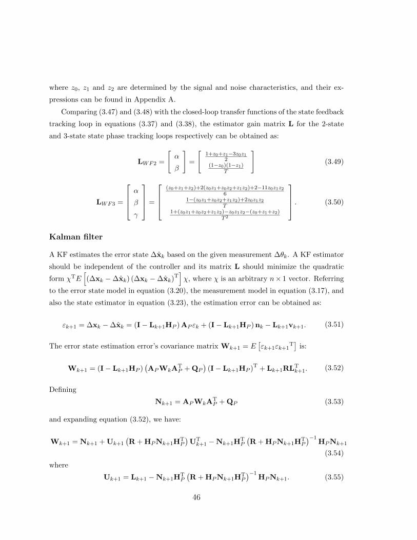
where z0, z1 and z2 are determined by the signal and noise characteristics, and their ex-
pressions can be found in Appendix A.
Comparing (3.47) and (3.48) with the closed-loop transfer functions of the state feedback
tracking loop in equations (3.37) and (3.38), the estimator gain matrix L for the 2-state
and 3-state state phase tracking loops respectively can be obtained as:
LWF2 =
[α
β
]=
[1+z0+z1−3z0z1
2(1−z0)(1−z1)
T
](3.49)
LWF3 =
α
β
γ
=
(z0+z1+z2)+2(z0z1+z0z2+z1z2)+2−11z0z1z2
61−(z0z1+z0z2+z1z2)+2z0z1z2
T1+(z0z1+z0z2+z1z2)−z0z1z2−(z0+z1+z2)
T 2
. (3.50)
Kalman filter
A KF estimates the error state ∆xk based on the given measurement ∆θk. A KF estimator
should be independent of the controller and its matrix L should minimize the quadratic
form χTE[(∆xk −∆xk) (∆xk −∆xk)
T]χ, where χ is an arbitrary n× 1 vector. Referring
to the error state model in equation (3.20), the measurement model in equation (3.17), and
also the state estimator in equation (3.23), the estimation error can be obtained as:
εk+1 = ∆xk −∆xk = (I− Lk+1HP )AP εk + (I− Lk+1HP )nk − Lk+1vk+1. (3.51)
The error state estimation error’s covariance matrix Wk+1 = E[εk+1εk+1
T]
is:
Wk+1 = (I− Lk+1HP )(APWkA
TP + QP
)(I− Lk+1HP )T + Lk+1RLT
k+1. (3.52)
Defining
Nk+1 = APWkATP + QP (3.53)
and expanding equation (3.52), we have:
Wk+1 = Nk+1 + Uk+1
(R + HPNk+1H
TP
)UTk+1 −Nk+1H
TP
(R + HPNk+1H
TP
)−1HPNk+1
(3.54)
where
Uk+1 = Lk+1 −Nk+1HTP
(R + HPNk+1H
TP
)−1HPNk+1. (3.55)
46

Hence the quadratic form χTWk+1χ is a minimum when Uk+1 = 0. Thus, KF gain matrix
can be obtained as:
Lk+1 = Nk+1HTP
(R + HPNk+1H
TP
)−1(3.56)
and the corresponding Wk+1 is:
Wk+1 = (I− Lk+1HP )Nk+1. (3.57)
The above analysis shows that the KF gain Lk+1 is the the gain matrix that minimizes
χTWk+1χ regardless of the matrices B, K and the controller uk. However, the error state
estimator is only a subsystem of the control system, see Fig.3.1. To obtain the performance
of the overall closed system with this error state estimator, we apply B = I, K = AP and
uk = K∆xk into equation (3.19):
xk+1 = AP xk + AP∆xk. (3.58)
The full state estimation variance can be derived from (3.1) and (3.58):
E[(xk+1 − xk+1) (xk+1 − xk+1)T
]= APWkA
TP + QP = Nk+1. (3.59)
Equation (3.59) shows that a minimal Wk corresponds to a minimal quadratic form
χTE[(xk+1 − xk+1) (xk+1 − xk+1)T
]χ; therefore the gain matrix Lk+1 in equation (3.56)
not only minimizes the error state estimation errors but also the full state estimation errors.
Since χ is an arbitrary n× 1 vector, we may choose χ = HTP :
χTE[(xk+1 − xk+1) (xk+1 − xk+1)T
]χ = HPE
[(xk+1 − xk+1) (xk+1 − xk+1)T
]HTP
= E[(θk − θk)2].
(3.60)
As a result, with B = I, K = AP , and uk = K∆xk and the KF gain matrix Lk+1, the
overall closed phase tracking loop operates at the MMSE tracking performance.
In the KF implementation, the gain update process is operated in two stages; namely,
the transient and the steady-state stage. Given an initial error covariance matrix W0, Lk+1
will converge to the constant optimal gain matrix as the system transits from the transient-
state to the steady-state. Letting LKF = limk→∞
Lk+1 denotes the steady-state KF gain. To
obtain LKF , we first solve the following discrete algebraic Riccati equation (DARE) to get
47

the steady-state covariance matrix N∞
APN∞ATP −APN∞HT
P
(HPN∞HT
P + R)−1
HPN∞ATP + QP −N∞ = 0. (3.61)
Substituting N∞ into equation (3.56), we obtain the numerical solutions of LKF .
Discussions and analysis
The gain matrix for PIF, WF, and KF provides a powerful analysis tool for their corre-
sponding designs and performances. In the PIF design, the values of LPIF in equations
(3.43) and (3.44) are primarily determined by the values of BN and T as shown in Table
2.1. Adjusting the value of BN is the most effective way to obtain the desired performance
for nominal signal tracking, i.e., increasing BN allows fast convergence in the transient-
state and decreasing BN achieves better tracking accuracy in the steady-state. For weak
signal tracking, the value of T should be increased to compensate for the power loss through
coherent or non-coherent accumulations [4,34]; in this case the value of BN should also be
adjusted accordingly. In practice, the values of BN and T are typically chosen based on the
empirical guidelines which do not provide rigorous analysis under different signal conditions.
In the WF design, LWF is a function of the characteristic roots as shown in equations
(3.49) and (3.50), where the locations of these roots are uniquely determined by the signal
and noise characteristics. Since the value of LWF is related to the signal model, with this
optimal gain, the WF-based tracking loop could achieve MMSE tracking performance in the
steady-state by design, which is superior compared to the heuristic nature of the PIF-based
tracking loop.
In the KF design, LKF is calculated from an iterative operation and determined by
the system characteristic matrices AP , HP , QP and R. With this gain the KF-based
tracking loop could achieve the MMSE performance with both the error state and full state
estimation.
Since WF and KF both generate estimations to minimize E[(θk − θk)2] under the as-
sumption of white Gaussian noise in the time-invariant linear systems, is it possible that
LWF and LKF are equivalent? If they are, then we may use LWF as the closed form repre-
sentation of steady-state LKF . To investigate the relationship between LWF and LKF and
the impact of the systematic characteristic matrices AP , HP , QP and R on the gain ma-
trices LWF and LKF , we compare the analytical solutions of LWF with numerical solutions
48
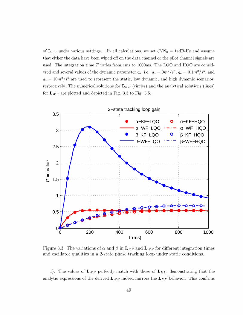
of LKF under various settings. In all calculations, we set C/N0 = 14dB-Hz and assume
that either the data have been wiped off on the data channel or the pilot channel signals are
used. The integration time T varies from 1ms to 1000ms. The LQO and HQO are consid-
ered and several values of the dynamic parameter qa, i.e., qa = 0m2/s5, qa = 0.1m2/s5, and
qa = 10m2/s5 are used to represent the static, low dynamic, and high dynamic scenarios,
respectively. The numerical solutions for LKF (circles) and the analytical solutions (lines)
for LWF are plotted and depicted in Fig. 3.3 to Fig. 3.5.
0 200 400 600 800 10000
0.5
1
1.5
2
2.5
3
3.5
T (ms)
Gai
n va
lue
2−state tracking loop gain
α−KF−LQOα−WF−LQO
β−KF−LQOβ−WF−LQO
α−KF−HQOα−WF−HQO
β−KF−HQOβ−WF−HQO
Figure 3.3: The variations of α and β in LKF and LWF for different integration timesand oscillator qualities in a 2-state phase tracking loop under static conditions.
1). The values of LWF perfectly match with those of LKF , demonstrating that the
analytic expressions of the derived LWF indeed mirrors the LKF behavior. This confirms
49

0 100 200 300 400 500 600 700 800 900 10000
1
2
3
4
5
6
7
T (ms)
Gai
n va
lue
3−state tracking loop gain with qa=0.1m2/s5
α−KF−HQOα−WF−HQOβ−KF−HQOβ−WF−HQOγ−KF−HQOγ−WF−HQO
α−KF−LQOα−WF−LQOβ−KF−LQO
β−WF−LQOγ−KF−LQOγ−WF−LQO
Figure 3.4: The variations of α, β, and γ in LKF and LWF for different integrationtime and oscillator qualities in a 3-state phase tracking loop under low dynamicconditions when qa = 0.1m2/s5.
that WF and KF are equivalent under the white Gaussian noise assumption in a time-
invariant linear system.
2). From the perspective of system noise, the values of α and β are higher for the
receiver with LQO than those with HQO. This indicates that the system modelling error
with a good quality oscillator is smaller than that of a poor quality oscillator. Therefore,
more weight should be given to estimation from system prediction for receivers with HQOs.
3). From the perspective of measurement noise, increasing the value of T effectively
reduces the measurement noise especially when the signal is weak. However, there is a
limit to the effective range of T values. The figures show that as T increases from 1ms
to 100ms, the loop gain parameters values are increased monotonically. For T >200 ms,
50

0 200 400 600 800 10000
5
10
15
20
25
30
T (ms)
Gai
n va
lue
3−state tracking loop gain with qa=10m2/s5
α−KF−HQOα−WF−HQOβ−KF−HQO
β−WF−HQOγ−KF−HQOγ−WF−HQO
α−KF−LQOα−WF−LQOβ−KF−LQO
β−WF−LQOγ−KF−LQOγ−WF−LQO
Figure 3.5: The variations of α, β, and γ in LKF and LWF for different integrationtime and oscillator qualities in a 3-state phase tracking loop under high dynamicconditions when qa = 10m2/s5.
the gain parameters subsequently decreases before reaching a steady level. Therefore, the
filter gain and the integration time are not always positively correlated. Moreover, long time
integration will cause some problems. For example, the oscillator phase noise is accumulated
with a longer integration time and the small errors of frequency estimation may lead to the
signal correlation loss. Hence, it is better to combine an appropriate integration time with
a well-designed filter to achieve equivalent or better tracking performance.
4). From the perspective of signal dynamics, the dynamic parameter qa has a greater
influence on the value of γ in LWF and LKF . From Fig.3.4 and Fig.3.5, it can be observed
that the value of γ increases drastically as qa increases, while the values of α and β are less
51

affected. For the special case qa = 0m2/s5, comparison of the QP matrix in equations (3.7)
and (3.8), shows that the 3-state model degrades to the 2-state model when γ = 0. Hence, γ
determines the ability of the filter to track dynamic signals. For the static scenario shown
in Fig.3.3, the value of α reaches its steady state level when T is about 600ms for a receiver
with HQO, while for a receiver with LQO, α reaches its steady state level when T is about
100ms. The reason is that increasing T in the receiver with LQO is not as effective as that
of HQO due to the larger oscillator noise. While the opposite cases are presented in the
dynamic scenarios as shown in Fig.3.4 and Fig.3.5, indicating that the receivers with HQO
are more sensitivity to platform dynamics than that with LQO.
3.4 Closed Form Performance Indicators and Per-
formance Analysis
In this section, the closed form expressions of phase tracking loop performance indicators in
terms of error covariance and mean error for the state feedback/state estimator representa-
tion of carrier tracking loops are derived. The tracking performance of the different tracking
designs, (i.e., PIF, WF and KF designs) under various operating situations, with varying
signal strength, platform dynamics, and oscillator qualities will be compared and analyzed.
In addition, the 3-sigma phase error rule will be applied to characterize the admissible range
of the loop parameters for tracking loop design implementation.
3.4.1 Tracking Performance Indicators
The most frequently used performance indicators for the GNSS applications are the expec-
tation and the variance of the state estimation errors. In this section, we derive closed-form
expressions of the corresponding performance indicators for the phase tracking loop with
B = I, K = AP , and different gain matrix representations of PIF, WF, and KF implemen-
tations.
Tracking error variance
Denote Pk+1 as the tracking error covariance matrix at the (k + 1)th epoch:
Pk+1 = E[(xk+1 − xk+1) (xk+1 − xk+1)T
]. (3.62)
52

Substituting the received and local generated signal in equations (3.1) and (3.33) into (3.62),
we have
Pk+1 = AP (I− LHP )Pk(I− LHP )TATP + QP + APLR(APL)T (3.63)
When k approaches infinity, the system reaches the steady-state, Pk+1 = Pk. Denoting the
steady-state error covariance as PX , for a given estimator gain matrix L, the closed-form
expression of PX can be obtained by solving equation (3.63). L can be LPIF , LWF and
LKF , and the corresponding PX is denoted as PPIF , PWF and PKF , can be obtained
accordingly. Note that LWF is equivalent to LKF , and PWF is identical to PKF which
converges to N∞ (see equation (3.59)). For the 3-state tracking model, the main diag-
onal elements PX represent the instantaneous estimation error for initial carrier phase,
frequency, and frequency rate, respectively. The remaining elements of PX denote the error
covariance between the state variables. The error variance of the overall average phase over
an integration time T can be obtained as
pθ = E
[(θk+1 − θk+1
)2]
= HPE[(xk+1 − xk+1) (xk+1 − xk+1)T
]HTP = HPPXH
TP .
(3.64)
Substituting equation (3.63) into (3.64), it can be seen that pθ is related to system char-
acteristics, such as oscillator error, platform dynamics, signal C/N0, and signal frequency
fL. Equation (3.64) also provides a quantitative relationship between the phase tracking
accuracy and design parameters, such as T or BN (if LPIF is adopted).
Dynamic stress steady-state error
When the receiver platform acceleration ak 6= 0m/s2, a steady-state error will occur in
the 2-state phase tracking loop. Similarly, when the receiver platform jerk jk 6= 0m/s3,
a steady-state error will occur in the 3-state phase tracking loop. Here, we derived the
dynamic stress error in the phase tracking loops for the dynamic scenarios having constant
acceleration or constant jerk. To reflect this dynamic, we add an input dynamic vector [72]
to the system model and obtain:
xk+1 = Axk + nk + Mdk (3.65)
53

where dk represents the platform LOS acceleration ak in the 2-state phase tracking loop or
LOS jerk jk in the 3-state phase tracking loop [72]
2− state : dk = ak(m/s2) (3.66)
3− state : dk = jk(m/s3). (3.67)
M is an operator that maps the dynamic input vector dk to the state vector, M for phase
tracking has the corresponding forms:
2− state : MP =[
2πfLc
T 2
22πfLTc
]T(3.68)
3− state : MP =[
2πfLc
T 3
62πfLc
T 2
22πfLTc
]T. (3.69)
Thus the average state error at (k + 1)th epoch can be expressed as
E (xk+1 − xk+1) = AP (I− LHP )E (xk − xk) + MPdk. (3.70)
Denoting eX = limk→∞
E (xk+1 − xk+1) as the steady-state error, we have
eX = [I−AP (I− LHP )]−1 MPdk. (3.71)
The steady-state dynamic stress phase error can be expressed as
eθ = limk→∞
E(θk+1 − θk+1
)= HP eX = HP [I−AP (I− LHP )]−1MPdk (3.72)
It can be seen that eθ is related to platform dynamics. Equation (3.72) also provides the
quantitative relationship between the dynamic stress error and design parameters, such as
T or BN (if LPIF is adopted).
3.4.2 Performance Analysis
The 3-sigma phase jitter [8] can be expressed as:
3σPLL = 3√pθ + eθ (3.73)
In traditional PLL design, a conservative rule of thumb requires that the 3-sigma phase
54

jitter does not exceed one-fourth of the phase pull-in range of the PLL discriminator [8]. For
the two-quadrant arctangent and four-quadrant discriminators in data and pilot channels,
the tracking error should satisfy the following conditions respectively [8]:
σPLL =√pθ +
eθ3≤ 15◦ or 30◦. (3.74)
We can observe that σPLL is related to the users’ dynamic, signal strength, oscillator quality,
and loop parameters. Therefore, to satisfy the above conditions, the loop parameters, should
be carefully designed to adapt to different environments to avoid loss of lock.
To compare the performance of these designs and to investigate the admissible range of
the loop parameters under the different signal strengths, platform dynamics, and oscillator
conditions, the value of σPLL with a 15◦ or 30◦ locked range of the phase tracking loops are
plotted in Fig.3.6 to Fig.3.9. In our analysis, the value of C/N0 is varied from 10dB-Hz to
44dB-Hz and the oscillators are chosen either as LQO or HQO. Several dynamic situations,
i.e., ak = 0m/s2 and ak = 1m/s2 in the 2-state phase tracking loops, jk = 0m/s3 and
jk = 1m/s3 in the 3-state phase tracking loops are considered, respectively. Since the
navigation data period for GPS L1 signal is 20ms, the integration time used in carrier
tracking loop is typically less than 20ms to avoid data bit transition. Here we assume that
the data have been wiped off for the data channel or the pilot channel signals are used and
the value of T varies from 1ms to 1000ms. The value of BN · T is set at 0.3 in PIF-based
phase tracking loop, and the value of qa is set at 0.1m2/s5 in the 3-state model. The curves
in Fig.3.6-3.9 represent the locus of (T ,C/N0) where the tracking error is 15◦ or 30◦. Some
conclusions can be drawn from these figures.
i). If there is no dynamic stress error, the 2-state and 3-state phase tracking loop results
are shown in Fig.3.6 and Fig.3.7, respectively. For the same C/N0, the admissible range
of T in the receiver with HQO is wider than that of the receiver with LQO, due to the
better clock characteristics for all phase tracking loop designs. Furthermore, the 15◦ and
30◦ locked range of the tracking loops with LWF and LKF are wider than that of the loop
with LPIF , since both LWF and LKF are the optimal gains in the sense of MMSE, which
ensures better tracking accuracy.
ii). If dynamic stress error exists, such as the velocity changes with a rate of 1m/s2 in
the 2-state phase tracking loop, as shown in Fig.3.8, or the acceleration changes with a rate
of 1m/s3 in the 3-state phase tracking loop, as shown in Fig.3.9, the admissible range of T
55

C/No (dB−Hz)
T (
ms)
(a). σPLL
< 15 (°)
10 15 20 25 30 35 40 44
200
400
600
800
1000
LQO−PIFLQO−WF/KF
C/No (dB−Hz)
T (
ms)
(b). σPLL
< 30 (°)
10 15 20 25 30 35 40 44
200
400
600
800
1000
HQO−PIFHQO−WF/KF
Figure 3.6: σPLL in 2-state phase track-ing loops for various receiver oscillatorqualities and tracking loop designs with-out dynamic stress error (a = 0m/s2)
C/No (dB−Hz)
T (
ms)
(a). σPLL
< 15 (°)
10 15 20 25 30 35 40 44
100
200
300
400LQO−PIFLQO−WF/KF
C/No (dB−Hz)
T (
ms)
(b). σPLL
< 30 (°)
10 15 20 25 30 35 40 44
100
200
300
400
HQO−PIFHQO−WF/KF
Figure 3.7: σPLL in 3-state phase track-ing loops for various receiver oscillatorqualities and tracking loop designs with-out dynamic stress error (j = 0m/s3)
C/No (dB−Hz)
T (m
s)
(a). σPLL
< 15 (°)
10 15 20 25 30 35 40 44
50
100
150LQO−PIFLQO−WF/KF
C/No (dB−Hz)
T (m
s)
(b). σPLL
< 30 (°)
10 15 20 25 30 35 40 44
50
100
150
HQO−PIFHQO−WF/KF
Figure 3.8: σPLL in 2-state phase track-ing loops for various receiver oscillatorqualities and tracking loop designs withdynamic stress error (a = 1m/s2)
C/No (dB−Hz)
T (m
s)
(a). σPLL
< 15 (°)
10 15 20 25 30 35 40 44
100
200
300
400LQO−PIFLQO−WF/KF
C/No (dB−Hz)
T (m
s)
(b). σPLL
< 30 (°)
10 15 20 25 30 35 40 44
100
200
300
400
HQO−PIFHQO−WF/KF
Figure 3.9: σPLL in 3-state phase track-ing loops for various receiver oscillatorqualities and tracking loop designs withdynamic stress error (j = 1m/s3)
56

is decreased, as can be seen by comparing Fig.3.6 and Fig.3.7. This observation indicates
that using a shorter integration time may increase the dynamic tracking ability, but at
the cost of tracking sensitivity. Additionally, the 15◦ and 30◦ locked range of the phase
tracking loops with LWF and LKF are decreased substantially when dynamic stress error
occurs as compared to the loop with LPIF , as can be seen in Fig.3.8 and Fig.3.9. The
reason is that PIF uses a model-free approach, where the filter parameters are designed
according to the empirical values, but WF/KF is a model-based approach, where the filter
is designed according to the system noise characteristic. As such, WF/KF results in a
narrower equivalent bandwidth which is able to eliminate the system noise more effectively
but at the cost of dynamic adaptability. It is known that the components α and β in
LWF and LKF are mainly determined by the oscillator characteristic, and γ is mainly
determined by the dynamic parameter qa. Hence, the design of LWF and LKF with poor
oscillator quality results in large values of α and β. In this case, the tracking loop with
LQO parameters is more robust than that of HQO parameters when the dynamic stress error
exists, as can be seen in Fig. 3.8. However, a different result arises when γ is introduced
in 3-state phase tracking loops with LWF and LKF , as shown in Fig. 3.9. With almost the
same value of γ, the tracking sensitivity of the loop with HQO is higher than that of the
receiver with LQO due to the smaller oscillator noise.
In summary, σPLL in equation (3.74) provide the admissible range of the loop parameters
under various operating situations, with varying signal strength, platform dynamics, and
oscillator qualities. If dk is non-zero, there will be a bias, such as eθ in phase tracking
loop that degrades the tracking performance. To avoid the performance degradation caused
by the dynamic stress error, additional state should be included in the state model to
account for this unknown constant bias. For example, under the constant acceleration
where dk = ak 6= 0m/s2, there will be a bias in 2-state phase tracking loop, while 3-
state phase tracking loop is unbiased because the additional state ωk is used to estimate
this bias. In this thesis, we assume that dk is zero for simplicity. To further improve
the tracking performance, the loop parameters that minimize pθ will be discussed in the
following section.
57

3.5 Optimization: Minimum Average Phase Track-
ing Error Variance Criteria
Analysis presented in Section 3.4 shows that the error variance, pθ, is determined by signal
strength, platform dynamics, receiver oscillator, and tracking loop gain matrix L. The
signal characteristics, which are determined by the external factors, can not be controlled.
However, the gain matrix L, is determined by the design specifications, such as the value
of integration time T and equivalent noise bandwidth BN (if PIF is adopted), and can be
optimized to improve the tracking accuracy. According to the analysis in Section 3.4, the
minimum tracking error variance could be achieved if the appropriate value of T is selected
for each specified signal strength and dynamics in the phase tracking loops with PIF, WF,
and KF designs. Similarly, the optimal value of BN could also be obtained which enables
higher tracking accuracy in the PIF-based phase tracking loop. Therefore, the objective in
this section is to investigate the optimal parameters that minimize the value of pθ in three
PLL designs employing PIF, WF, and KF for GPS L1 signals.
In the optimization procedure, several typical situations: weak and strong signal strength
(C/N0 = 10 ∼ 44dB-Hz), low and highly dynamics (qa = 0, 0.1, 1, 10, 100, 1000m2/s5), LQO
and HQO effects are considered. The value of T varies from 1ms to 1000ms in PIF-, WF-,
and KF-based phase tracking loops and the maximum value of BN · T is set at 0.5 in PIF-
based phase tracking loop. Under these given conditions, the optimal values of T , Topt, can
be obtained by minimizing pθ in the PIF-, WF-, and KF-based phase tracking loops accord-
ingly. Besides, the values of BNopt for a PIF-based phase tracking loop can be obtained by
dividing the BN ·T that minimizes pθ by Topt as well. With these optimal loop parameters,
the minimum phase tracking error variance, pθmin, in these three phase tracking loops could
be investigated and compared. The corresponding values of Topt,√pθmin, and BNopt are
plotted in Fig. 3.10-3.13 accordingly.
For a static receiver as shown in Fig. 3.10, the phase tracking error is dominated by
thermal noise and oscillator noise and Topt should be chosen to balance them. The followings
can be observed from Fig. 3.10:
i). The value of Topt increases as the signal C/N0 decreases especially when the C/N0
is low.
ii). Topt for the receiver with a HQO is larger than that of the receiver with a LQO.
The higher oscillator quality results in a ∼9dB improvement in tracking sensitivity if 15◦
58

10 15 20 25 30 35 40 440
50
100
150
200
C/No (dB−Hz)
T opt (m
s)
(a)
LQO−PIFLQO−WF/KFHQO−PIFHQO−WF/KF
10 15 20 25 30 35 40 440
20
40
60
C/No (dB−Hz)
p θ−0.5 m
in (°
)
(b)
15°
30°
Figure 3.10: Topt and√
pθmin versus C/N0 for both high and low receiver oscillatorqualities for 2-state phase tracking loop with PIF, WF, and KF designs under thestatic condition.
threshold is used.
iii). For Topt and√pθmin the difference between PIF- and WF/KF- based phase tracking
loops are barely noticeable, which indicates that based on the same cost function, i.e.,
minimizing pθ, there is only one optimal design regardless of the specific filter design.
For a receiver on a dynamic platform, the effects of oscillator noise are not as significant
as for a static receiver, and Topt is chosen to balance the dynamic and the thermal noise
effect in phase tracking loop design. Fig. 3.11 and Fig. 3.12 show that:
i). The oscillator noise effect becomes less important when the dynamics is increased.
Topt and√pθmin for receivers with LQO and HQO gradually overlap for both the low and
highly dynamic cases, as the C/N0 decreases.
ii). As the dynamic increases, Topt decreases while√pθmin increases. In a receiver with
HQO at 10dB-Hz signal strength, a WF/KF-based PLL operating with Topt at a ∼80ms
could obtain a ∼ 50◦ MMSE performance under low dynamic conditions, while under highly
59

10 15 20 25 30 35 40 440
20
40
60
80
100
C/No (dB−Hz)
T opt (m
s)
(a)
LQO−PIFLQO−WF/KFHQO−PIFHQO−WF/KF
10 15 20 25 30 35 40 440
20
40
60
80
C/No (dB−Hz)
p θ−0.5 m
in (°
)
(b)
15°
30°
Figure 3.11: Topt and√
pθmin versus C/N0 for both high and low receiver oscillatorqualities for 3-state phase tracking loop with PIF, WF, and KF designs under thelow dynamic condition (qa = 0.1m2/s5).
Table 3.1: Theoretical PLL tracking sensitivities with thresholds of 15◦ (data channel)and 30◦ (pilot channel) values for static, low, and high signal dynamics, both highand low receiver oscillator qualities, and the optimal PIF-, WF-, and KF-based phasetracking loop designs (unit: dB-Hz)
qa(m2/s5)
LQO HQOPIF WF/KF PIF WF/KF
0 22/15 22/15 13/6 13/60.1 23/17 23/16 21/15 21/141 24/18 23/17 23/17 23/1610 26/19 25/19 25/19 25/18100 27/21 27/21 27/21 27/211000 29/23 29/22 29/23 29/22
Note: */* represent the corresponding phase tracking loop sensitivity with respect to15◦/30◦ threshold;
60

10 15 20 25 30 35 40 440
20
40
60
C/No (dB−Hz)
T opt (
ms)
(a)
LQO−PIFLQO−WF/KFHQO−PIFHQO−WF/KF
10 15 20 25 30 35 40 440
50
100
C/No (dB−Hz)
p θ−0.5 m
in (°
)
(b)
15°
30°
Figure 3.12: Topt and√
pθmin versus C/N0 for both high and low receiver oscillatorqualities for 3-state phase tracking loop with PIF, WF, and KF designs under thehighly dynamic condition (qa = 10m2/s5).
dynamic conditions Topt is ∼50ms, and the corresponding minimum phase tracking error is
∼ 80◦, indicating that higher dynamic limits integration times, degrades tracking accuracy,
as well as tracking sensitivity.
iii). The minimum tracking errors in PIF-based phase tracking loops are slightly larger
than that in WF- and KF-based phase tracking loops under both low and highly dynamic
conditions. As was discussed in Section 3.3, for LPIF , its components, α, β, and γ, are
determined by the values of BN and T , while for LWF and LKF , their α and β are mainly
determined by the oscillator h−parameters and T , and γ is determined by qa and T . The
value of γ is coupled with α and β in LPIF , but is independent of α and β in LWF and
LKF . This allows a higher degree of freedom in the WF- and KF-based phase tracking loop
designs. Hence, PIF-based phase tracking loop only achieves a sub-optimal performance,
while the optimizations of WF- and KF-based phase tracking loops can realize the MMSE
performance.
61

10 15 20 25 30 35 40 440
5
10
15
20
25
30
35
C/No (dB−Hz)
BN
opt (H
z)
qa= 0 m2/s5
qa=0.1m2/s5
qa=10 m2/s5
qa= 0 m2/s5
qa=0.1m2/s5
qa=10 m2/s5
HQO
LQO
Figure 3.13: BN opt dependency on C/N0 for static, low, and high signal dynamics,both high and low receiver oscillator qualities in the PIF-based phase tracking loop.
Fig.3.13 shows that:
i). BNopt increases as the signal C/N0 increases.
ii). BNopt in a receiver with LQO is wider than that in a receiver with HQO.
iii). BNopt increases as receiver dynamics increase. These trends are opposite to that
of Topt in Fig.3.10-3.12. This is because for a stronger signal, a shorter integration time is
needed, so a larger loop bandwidth can be accommodated to handle the higher dynamics
and the larger oscillator noises.
Tracking sensitivity refers to the tracking capability of the weak signal in GNSS receiver.
Here, we assume that the tracking loop could maintain lock when the tracking error is below
the tracking threshold, such as 15◦ for data channel and 30◦ for pilot channel. The tracking
sensitivity represents the lowest signal C/N0 that can be tracked by the phase tracking
loops without loss-of-lock. The theoretical tracking sensitivities of the generalized phase
tracking loops with optimal loop parameters, i.e., Topt and BNopt, according to the 3-sigma
62

Table 3.2: Topt and BNopt parameter values for static, low, and high signal dynamics,both high and low receiver oscillator qualities, and PIF-, WF-, and KF-based phasetracking loop designs
qa(m2/s5) Oscillator
qualityTracking loop
typeb1 µ1 b2 µ2
0Low
PIF 0.257 0.559 1.191 0.288WF/KF 0.272 0.567 N/A
HighPIF 0.700 0.583 0.313 0.258
WF/KF 0.719 0.588 N/A
0.1Low
PIF 0.166 0.527 1.677 0.278WF/KF 0.247 0.555 N/A
HighPIF 0.190 0.487 1.981 0.179
WF/KF 0.279 0.526 N/A
1Low
PIF 0.140 0.501 2.212 0.251WF/KF 0.211 0.537 N/A
HighPIF 0.140 0.473 2.858 0.181
WF/KF 0.213 0.514 N/A
10Low
PIF 0.103 0.467 3.597 0.213WF/KF 0.163 0.511 N/A
HighPIF 0.104 0.459 4.110 0.183
WF/KF 0.163 0.502 N/A
100Low
PIF 0.076 0.448 5.662 0.193WF/KF 0.121 0.492 N/A
HighPIF 0.074 0.438 5.910 0.184
WF/KF 0.124 0.493 N/A
1000Low
PIF 0.052 0.416 8.271 0.191WF/KF 0.092 0.482 N/A
HighPIF 0.052 0.415 8.433 0.187
WF/KF 0.090 0.473 N/A
rule are summarized in Table 3.1. The values in Table 3.1 shows that:
i). Under the static scenario (qa = 0m2/s5), a phase tracking loop tracking sensitivity
mainly depends on the receiver oscillator quality. The theoretical tracking sensitivity for a
receiver with a HQO is as low as 13dB-Hz and 6dB-Hz for data channels and pilot channels,
respectively, which is ∼ 9dB higher than that for a receiver with LQO. These are the
theoretical upper bounds of phase tracking loop tracking sensitivity.
ii). Under the dynamic scenario (qa 6= 0m2/s5), the influence of oscillator quality
63

becomes less important as the platform dynamics increases. The tracking sensitivity for a
receiver with a LQO is the same as one with a HQO when qa > 1m2/s5. The higher the
platform dynamics, the worse the tracking sensitivity becomes.
iii). Although a phase tracking loop with LPIF is suboptimal, it can still achieve nearly
the same tracking sensitivity as the ones with LWF and LKF . This indicates that under the
uniform optimization criteria, the phase tracking loop performance is mainly limited by the
signal characteristics and receiver hardware quality, such as oscillator quality and platform
dynamics, regardless of what filter design is used.
iv). There is a general 6dB to 7dB improvement in pilot channels over data channels.
The potential advantages of pilot channels over data channels are not greatly affected by
the receiver oscillator quality and platform dynamics, as well as filter designs. These results
are consistent with the conclusions in
0 0.1 1 10 100 10000
0.2
0.4
0.6
0.8
b 1
qa(m2/s5)
Topt
=b1(C/No)−µ
1 (s)
0
0.2
0.4
0.6
0.8
0 0.1 1 10 100 10000
0.2
0.4
0.6
0.8
µ 1
0
0.2
0.4
0.6
0.8
0 0.1 1 10 100 10000
0.2
0.4
0.6
0.8
µ 1
LQO−PIFHQO−PIFLQO−WF/KFHQO−WF/KF
LQO−PIFHQO−PIFLQO−WF/KFHQO−WF/KF
Figure 3.14: Trends of b1 and µ1 versus signal dynamics for high and low receiveroscillator quality, and phase tracking loop with PIF, WF, and KF designs.
To calculate the optimal values of Topt and BNopt for various signal scenarios, we obtain
the minimum value of pθmin over the search space of T from 1ms to 1000ms, BN · T from
0.0001 to 0.5, and C/N0 from 10dB-Hz to 44dB-Hz for each specified dynamics. These
64

0 0.1 1 10 100 10000
2
4
6
8
10
b 2
qa(m2/s5)
BNopt
=b2(C/No)µ2 (Hz)
0
0.2
0.4
0.6
0.8
1
0 0.1 1 10 100 10000
µ 2
LQO−PIFHQO−PIF
LQO−PIFHQO−PIF
Figure 3.15: Trends of b2 and µ2 versus signal dynamics for high and low receiveroscillator qualities in the PIF-based phase tracking loop.
optimal values are uniquely associated with a given set of signal conditions and can be pre-
determined. Therefore, for practical applications, the relationships between Topt and C/N0,
BNopt and C/N0 can be established beforehand. Such relationships also provide insights
into the influence signal parameters have on the design choices. The relationships can be
summarized below:
Topt = b1(C/N0)−µ1(s) (3.75)
BNopt = b2(C/N0)µ2(Hz) (3.76)
where the parameters b1, µ1, b2, and µ2 for various signal dynamics, receiver oscillator
qualities, and phase tracking loop designs are obtained through curve fitting of numerical
calculations and listed in Table 3.2. Fig.3.16 shows an example of curve fitting of Topt versus
C/N0 for qa = 1m2/s5 in the receiver with low quality oscillator and WF/KF design. This
curve fitting guarantees 95% confidence degree. Equations (3.75) and (3.76) provide the
optimal parameter designs in the generalized phase tracking loop under diverse dynamic
and weak signal scenarios. To clearly show the trends of these parameters versus different
65

signal dynamics with various receiver oscillator qualities, and phase tracking loop designs,
their values are plotted in Fig.3.14 and Fig.3.15. [8].
Figure 3.16: Curve fitting example of Topt versus C/N0 for qa = 1m2/s5 in the receiverwith low quality oscillator and WF/KF design.
Fig.3.14 shows that as dynamic parameter qa increases, b1 and µ1 will decrease for both
LQO and HQO. Fig.3.15 shows that with the increasing of dynamic parameter qa, there is
a slight decline in µ2, and a sharp rise in b2. This indicates that the parameter b2 is more
sensitive to the changing signal dynamics. Similarly, the difference between b2 and µ2 for
low and high oscillator qualities is reduced with increasing signal dynamics.
3.6 Adaptive Phase Tracking Process
The typical phase tracking loops can be classified as a fixed L and fixed T (FL-FT) algorithm
or an adaptive L and fixed T (AL-FT) algorithm, respectively. The FL-FT approach
corresponds to the traditional PIF-based phase tracking loop, where L is determined by
the predefined value of BN and T . The AL-FT approach corresponds to the KF-based
phase tracking loop, where L is adjustable, based on the signal strength’s and platform
66

dynamics estimations, while the value of T is usually predefined and constant. When the
signal changes in a real environment, the tracking loop should be flexible enough to respond
accordingly, such that the value of T should be increased or decreased when the signal is
weak or strong under different dynamic scenarios. Based on the optimization analysis under
the assumption of white Gaussian noise, we apply these optimal designs in an adaptive phase
tracking loop, where the values of Topt in PIF, WF, and KF and BNopt in PIF are adaptively
tuned according to the variation of signal strength and dynamics to achieve the optimal
phase tracking loop sensitivity and accuracy.
The proposed adaptive tracking scheme requires knowledge of the signal C/N0 and dy-
namic characteristics. C/N0 can be obtained by using real time signal-to-noise ratio (SNR)
estimator at regular intervals [104–106]. A common approach is to utilize averaging times
on the order of a navigation data bit, or 20ms to achieve the lowest expected measurable
C/N0 estimates on the order of approximately 17dB-Hz [104]. The dynamics parameter qa
can be estimated directly using receiver measurements or other on-board sensors. Thus, by
using this relationship in equation (3.12), we can set the corresponding value of qa according
to the empirical knowledge of the platform’s dynamics.
In our proposed adaptive phase tracking algorithm (see Algorithm 1), T and other loop
parameters are adaptively tuned according to the estimations of C/N0 and qa to achieve
optimal tracking loop sensitivity and accuracy. Below is a summary of the processes in
Algorithm 1:
Assuming the C/N0 and qa are available, the adaptive tracking algorithm can be imple-
mented as follows:
1) Initialization. The tracking loop is initialized with Doppler frequency, carrier phase,
and C/N0 estimation from the acquisition process. In this initial stage, phase tracking loop
is operating with a 1ms integration time, and large loop bandwidth values (for example
BN ≥ 50Hz) are adapted to ensure fast convergence to the steady state.
2) Optimal tracking. When the phase tracking loop operates in a steady state, the
Topt and BNopt are obtained according to knowledge of C/N0 and qa estimations through
equations (3.75) and (3.76). The corresponding loop gain LPIF /LWF /LKF are calculated
and used to update the state estimations, which are subsequently used to generate Toptms
carrier signals (we assume that the data is wiped off when T > 1ms on data channel) for
correlation with new incoming signals, in phase discriminator calculation, and estimating
the signal C/N0 for preparation of the next tracking iteration.
67

3) Update. The integration time and loop parameters computed from 2) are updated
when a new C/N0 estimation is obtained in each new epoch. Otherwise, the loop parameters
are kept unchanged until C/N0 is updated.
Consequently, the adaptive phase tracking loop adjusts the values of T and L in an
time-varying manner aimed to achieve the theoretical MMSE performance. Noted that in
a fading environment, this algorithm may not work if the fading is faster than the C/N0
estimation time interval.
Algorithm 1 Adaptive phase tracking algorithm
1: Initialization:2: Set T = 1ms and calculate the phase error ∆θk from the phase discriminator
once per 1ms;3: Set BN = 50Hz to make the tracking loop fast convergent to steady-state;4: Obtain the value of C/N0 estimation, c/n0, through the SNR estimator;5: Optimal tracking:6: Set T = Topt, where Topt = b1(c/n0)−µ1 ;7: Set BN = BNopt, where BNopt = b2(c/n0)µ2 (if PIF is adopted);8: Calculate the loop gain matrix L, such as LPIF , LWF , and LKF ;9: Calculate the phase error ∆θk from the phase discriminator once per Toptms;
10: Estimate the state xk+1 = AP xk + APL∆θk once per Toptms;11: Generate Toptms carrier signals for correlation and estimate the signal C/N0;12: Update:13: if c/n0 is not changed then14: go to line 9;15: else16: go to line 6;17: endif
68

Chapter 4
State feedback/state estimator
design for frequency tracking loop3
Frequency tracking is essentially differential carrier phase tracking that neglects absolute
phase error and permits relative phase rotation between the received signal and the local
carrier replica [8]. Hence, a FLL can be treated as a reduced-order PLL, where a first-order
or a second-order FLL achieves the equivalent frequency tracking capability as a second-
order or a third-order PLL respectively.
In this Chapter, the general state space design control system process in Chapter 2 is
applied in frequency tracking loop design. The detailed frequency tracking loop design and
analysis follow the same approach as that of the generalized phase tracking loop design in
Chapter 3.
3Chapter 4 is the frequency tracking loop part of our papers “R. Yang, KV Ling, EK Poh, andY.Morton, Generalized GNSS Signal Carrier Tracking: Part I: Modelling and Analysis, accepted byIEEE Transactions on Aerospace and Electronic Systems, January 2017. ” and “R. Yang, Y.Morton,KV Ling, and EK Poh, Generalized GNSS Signal Carrier Tracking: Part II: Optimization andImplementation, accepted by IEEE Transactions on Aerospace and Electronic Systems, January2017.”
69

4.1 Signal Model
Similar to the system model in phase tracking loop in Chapter 3, we have the following
system model for frequency tracking loop:
xk+1 = AFxk + nk (4.1)
zk = HFxk + vk (4.2)
to incorporate the platform dynamics, oscillator noise, and thermal noise effects into these
models. We use these models to design the generalized frequency tracking loop in state
space.
4.1.1 State model
In GNSS receivers, PLLs replicate the exact phase and frequency of the incoming signal to
enable carrier wipe-off from the incoming signals, while FLLs perform the carrier wipe-off
process by replicating the approximate frequency and allowing the replicate phase to rotate
with respect to the incoming carrier signal [8]. Thus, only the estimation of the frequency
ωk and frequency rate ωk are required in frequency tracking loop design. For this reason,
we adopt the following state vectors:
1− state : xk = ωk (4.3)
2− state : xk =[ω ω
]T
k(4.4)
to represent the input signals associated with typical dynamics of a GNSS receiver.
Similar to the state model of phase tracking loop in Chapter 3, we have the corresponding
reduced-order system transition matrix in frequency tracking loop:
1− state : AF = 1 (4.5)
2− state : AF =
[1 T
0 1
](4.6)
70

and the associated noise covariance matrix:
1− state : QF = σ2ω = (2πfL)2Tqω (4.7)
2− state : QF =
[σ2ω σ2
ωω
σ2ωω σ2
ω
]= (2πfL)2
[Tqω + T 3
3qac2
T 2
2qac2
T 2
2qac2
T qac2
](4.8)
4.1.2 Measurement model
In frequency tracking loop, the measurement can be obtained through the arctangent fre-
quency discriminator, using dot and cross products [8]:
∆$k+1 =1
Tarc tan (cross, dot)
=1
Tarc tan
(IPkQPk+1 − IPk+1QPkIPkIPk+1 +QPkQPk+1
)=
1
Tarc tan
(QPk+1/IPk+1 −QPk/IPk
1 + (QPk+1/IPk+1) (QPk/IPk)
)=
1
Tarc tan
(tan (∆θk+1)− tan (∆θk)
1 + tan (∆θk+1) tan (∆θk)
)=
1
Tarc tan (tan (∆θk+1 −∆θk))
=1
T(∆θk+1 −∆θk)
(4.9)
Generally, the two-quadrant and four-quadrant arctangent FLL discriminators are adopted
in generic receiver design for signals with and without navigation message modulations [3,8].
The frequency trackings of GNSS receivers must be insensitive to 180◦ reversals in the IPk
and QPk signals. Therefore, the sample times of the IPk and QPk signals should not straddle
the data bit transitions [17]. The maximum integration time of frequency tracking is 10ms
for GPS L1 signal to avoid the data bit transition for channels with data modulation.
Substituting equations (3.17) into equation (4.9) (see derivation in Appendix B), we can
obtain
1− state : ∆$k = ∆ωk +vk − vk−1
T(4.10)
2− state : ∆$k = ∆ωk +T
2∆ωk +
vk − vk−1
T. (4.11)
71

Denote the vector xk as the local estimation of xk and uk = (vk − vk−1)/T , the frequency
discriminator output ∆$k can be formulated as
∆$k = HF (xk − xk) + uk (4.12)
where uk is a non-white frequency measurement noise and HF is the frequency tracking
loop measurement matrix with the frequency forms:
1− state : HF = 1 (4.13)
2− state : HF =[
1 T2
]. (4.14)
4.2 Generalized Frequency Tracking Loop Design
Denote $k∆= $ + uk
∆= HFxk + uk as the system input and $k
∆= HF xk as the system
output in frequency tracking loop. The block diagram of the generalized frequency tracking
loop is shown as Fig. 4.1.
+Local
Reference
Generator
HF+-
Error State
EstimatorK
HF+
ku
kXˆkX
ku
ˆkX
ˆk k
k
Figure 4.1: Generalized frequency tracking loop architecture
Similar to the state space design for phase tracking loop in Chapter 3, the local reference
generator in frequency tracking loop is controlled by the controller uk:
xk+1 = AF xk + Buk. (4.15)
72

uk is designed by adopting the state feedback strategy as
uk = K∆xk (4.16)
And a state estimator need to be constructed based on the measurement ∆$k as the true
state information is not available:
∆xk = AF∆xk−1 −Buk−1 + L (∆$k −HF (AF∆xk−1 −Buk−1)) (4.17)
where L is the estimator gain matrix in frequency tracking loop.
Following the analysis in Chapter 3, we choose B = I and K = AF to simplify the error
state estimation in equation (4.17) and the corresponding state estimation can be obtained
as
xk+1 = AF xk + AFL∆$k. (4.18)
4.3 Estimator Gain Matrix Design
In generalized phase tracking loop design in Chapter 3, the gain matrices for three filter
designs, i.e.,PIF, WF, and KF are analyzed. Under the white Gaussian noise assumption,
LWF and LKF are both the optimal gain matrix that enables MMSE performance in phase
tracking loop. However, the frequency measurement noise uk in frequency tracking loop is
not a white noise. KF is not an optimal filter in the sense of MMSE for a FLL, although it
has been used in FLL design in [30], and it is also too complicated to obtain the closed-form
LWF for a FLL. Since the PIF is a model-free design approach that is immune to the noise
characteristic, we only consider the PIF design in the generalized frequency tracking loop
analysis and the gain matrix for a PIF is obtained by mapping the PIF-based frequency
tracking loop into the state space architecture through the equivalent closed-loop transfer
function discussed in Chapter 2.
The 1- and 2-state forms for L are:
1− state : L = α
2− state : L =[α β
]T.
(4.19)
The corresponding closed-loop transfer function between output $k and input $k in
73
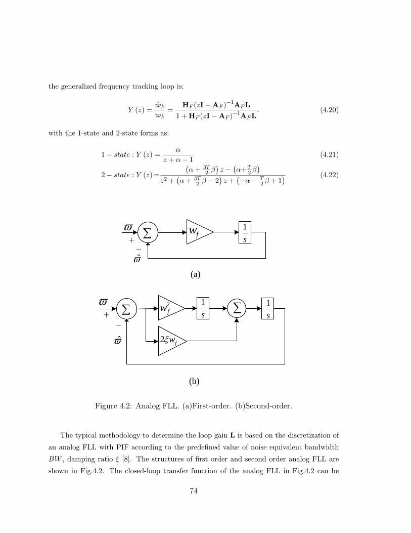
the generalized frequency tracking loop is:
Y (z) =$k
$k=
HF (zI−AF )−1AFL
1 + HF (zI−AF )−1AFL. (4.20)
with the 1-state and 2-state forms as:
1− state : Y (z) =α
z + α− 1(4.21)
2− state : Y (z) =
(α+ 3T
2 β)z −
(α+T
2 β)
z2 +(α+ 3T
2 β − 2)z +
(−α− T
2 β + 1) (4.22)
1
s
1
s
2
fw
2 fw
1
sfw
(a)
(b)
+-
+-
Figure 4.2: Analog FLL. (a)First-order. (b)Second-order.
The typical methodology to determine the loop gain L is based on the discretization of
an analog FLL with PIF according to the predefined value of noise equivalent bandwidth
BW , damping ratio ξ [8]. The structures of first order and second order analog FLL are
shown in Fig.4.2. The closed-loop transfer function of the analog FLL in Fig.4.2 can be
74

obtained as:
1− state : H (s) =$
$=
wfs+ wf
(4.23)
2− state : H (s) =$
$=
2ξwfs+ w2f
s2 + 2ξwfs+ w2f
(4.24)
where wf is the natural frequency in frequency tracking loop and can be calculated with
predefined value of BW as shown in Table 2.1.
By using the forward Euler transformation s = (z−1)/T , we discretize equations (4.23)
and (4.24) from the s-domain to the z-domain and obtain equations (4.25) and (4.26),
respectively.
1− state : H (z) =wfT
z + wfT − 1(4.25)
2− state : H (z) =2ξwfTz + w2
fT2 − 2ξwnT
z2 + (2ξwfT − 2) z +(w2fT
2 − 2ξwfT + 1) . (4.26)
Comparing the closed loop transfer functions of generalized frequency tracking loop in
equations (4.21) and (4.22) with that of the analog FLL in equations (4.25) and (4.26), the
gain matrix L for 1-state and 2-state generalized frequency tracking loops can be obtained
as
1− state : L = wfT (4.27)
2− state : L =
[2ξwfT − 3
2w2fT
2
w2fT
]. (4.28)
Note that the PIF design presented here is based on predefined empirical values of loop
parameters. It does not provide the rigorous design process for the loop parameters under
different signal conditions, especially in harsh environments where the signal is both weak
and on a highly dynamic platform. The performance analysis and optimization for the
generalized frequency tracking loop design will be presented next.
75
4.4 Performance Analysis
In this section, we derive the closed-form expressions of the frequency tracking error covari-
ance matrix and dynamic steady stress error for the generalized frequency tracking loop.
4.4.1 Estimation error variance
Denote Pk+1 as the tracking error covariance matrix at k + 1th epoch which can be expressed
as follows
Pk+1 = E[(xk+1 − xk+1) (xk+1 − xk+1)T
]. (4.29)
Substituting the received and local generated signal in equations (4.1), and (4.18) into
(4.29), we have (see derivation in Appendix C)
Pk+1 = AF (I− LHF )Pk(I− LHF )TATF + QF + 2AFL
R
T 2(AFL)T
−AF (I− LHF )Gk(AFL)T −AFLGTk (I− LHF )TAT
F
(4.30)
where Gk = E[∆xkuk
T]
and GTk = E
[uk∆xk
T]
represent the correlation between the
error state and non-white measurement noise.
At steady state, Pk+1 = Pk = PY and Gk+1 = Gk = GY as (see derivation in Appendix
C):
GY =AFL
T 2σ2v (4.31)
and
PY = AF (I− LHF )Pk(I− LHF )TATF + QF + 2AFL(AFL)T σ
2v
T 2
−AF (I− LHF )AFL(AFL)T σ2v
T 2−AFL(AFL)T(I− LHF )TAT
F
σ2v
T 2.
(4.32)
Denote pω as the overall average frequency error variance, we can get:
pω = HFE[(xk+1 − xk+1) (xk+1 − xk+1)T
]HTF = HFPYH
TF . (4.33)
Substituting equation (4.32) into (4.33), it can be seen that pω is again related to system
characteristics, such as oscillator error, platform dynamics, signal C/N0, and signal fre-
quency fL. Like equation (3.64), equation (4.33) also provides a quantitative relationship
76

between the frequency tracking accuracy and design parameters, such as T or BW .
4.4.2 Dynamic stress steady state error
When the platform velocity or acceleration changes, a steady state error will occur in both
the 1-state or 2-state frequency tracking loops. To reflect this change, similar to [72], we
add an input dynamic vector to the system model and obtain
xk+1 = Axk + nk + Mdk (4.34)
where dk represents the user’s LOS acceleration ak in the 1-state frequency tracking loop
or LOS jerk jk in the 2-state frequency tracking loop
1− state : dk = ak(m/s2) (4.35)
2− state : dk = jk(m/s3). (4.36)
M for frequency tracking has the corresponding forms:
1− state : MF =2πfLT
c
2− state : MF =[
2πfLc
T 2
22πfLTc
]T.
(4.37)
Denote eY = limk→∞
E (xk+1 − xk+1) as the frequency dynamic stress steady-state error when
k approaches to infinity, we have
eY = [I−AF (I− LHF)]−1MFdk. (4.38)
Hence, the overall dynamic stress frequency error can be expressed as
eω = limk→∞
E ($k+1 − $k+1) = HF eY = HF [I−AF (I− LHF )]−1MFdk. (4.39)
eω also dependent on platform dynamics and signal frequency fL. Equation (4.39) also pro-
vides the quantitative relationship between the dynamic stress error and design parameters,
such as T or BW .
77
4.4.3 The 3-sigma rule
In traditional FLL design, a conservative rule of thumb is usually applied to determine
the tracking threshold of FLL, which requires that the 3-sigma frequency jitter must not
exceed one-fourth of the frequency pull-in range of the FLL discriminator [8]. Therefore,
for the two-quadrant arctangent and four-quadrant frequency discriminators in data and
pilot channels, the tracking error should satisfy the following conditions respectively [8]:
σFLL =√pω +
eω3≤ 1
24T(Hz) or
1
12T(Hz) (4.40)
Equation (4.40) can be applied to characterize the admissible range of the loop parameters
such as T or BW for tracking loop design implementation under various operating situation-
s, with varying signal strength, platform dynamics, and oscillator qualities. The maximum
value of T is 10ms in GPS data channel to avoid the data bit transition. Equation (4.40)
shows that as the value of T increases from 1ms to 10ms, the threshold for the pilot channel
decreases from 83.3Hz to 8.33Hz. A shorter integration time is also preferred because the
threshold decreases as the value of T increases. The further improvement of the frequency
tracking performance that minimize pω will be discussed in the following section.
4.5 Optimization: Minimum Average Frequency
Tracking Error Variance Criteria
Similar to the case with phase tracking loop, the minimum frequency tracking error variance
for a frequency tracking loop could be achieved if the appropriate value of gain matrix L
is selected for each specified signal strength and receiver platform scenario. The objective
of optimization for generalized frequency tracking loop is to determine system parameters
that minimize the value of pω for the generalized frequency tracking loop design. For a
frequency tracking loop operating on a data channel, at least two integrated and dump
samples must be taken between data bit transitions, navigation data rate limits the length
of the integration time in frequency tracking loop and the maximum value of T for GPS L1
signal frequency tracking is 10ms. Even for pilot channel, a shorter integration time is also
preferred in a FLL because the threshold decreases as the value of T increases. Hence, two
cases that T = 1ms and 10ms are considered for frequency tracking loop optimization and
78

the corresponding optimal parameter, BWopt, will be analyzed.
4.5.1 1-state frequency tracking loop
Substituting AF , HF , QF , R and L into equation (4.33), we can get:
pω =(2πfL)2Tqω + 2σ2
v/T2α3
2α− α2. (4.41)
The extreme values of the function are the points where the partial derivatives are zero.
We take a derivative with respect to α and obtain:
dpωdα
=−2σ2
v/T2α4 + 8σ2
v/T2α3 + 2(2πfL)2Tqω(α− 1)
α2(α− 2)2 (4.42)
The derivative becomes zero when
−2σ2v/T
2α4 + 8σ2v/T
2α3 + 2(2πfL)2Tqω(α− 1) = 0. (4.43)
Let b = (2πfL)2 T 3qω/σ2v , then α4 − 4α3 − bα + b = 0. The solution that minimizes the
value of pω is (see derivation in Appendix D)
αopt = 1 +1
2
√4 +
3√b2 + 16b− 1
2
√8− 3
√b2 + 16b+
2b+ 16√4 + 3√b2 + 16b
. (4.44)
According to the relationship between α and BW in equation (4.27) and Table 2.1, we can
obtain the optimal value of BWopt as:
1− state : BWopt =αopt4T
. (4.45)
4.5.2 2-state frequency tracking loop
Due to the complexity involved in obtaining the analytical solutions of BW opt for the 2-
state case, the numerical solutions are provided here instead. The following scenarios are
considered: C/N0 = 10 ∼ 44dB-Hz and qa = 0.1, 1, 10, 100, 1000m2/s5 in the receiver with
LQO and HQO. T is set at 1ms and 10ms, and the maximum value of BW · T is 0.5. To
calculate the optimal values of BW opt for various signal scenarios, we obtain the minimum
79
value of pωmin over the search space of BW · T from 0.0001 to 0.5, and C/N0 from 10dB-
Hz to 44dB-Hz for each specified dynamics. Then, the corresponding values of BWopt can
be obtained by dividing the optimal product BW · T that minimizing pω by T = 1ms or
T = 10ms accordingly. As an example, the values of BW opt and√pωmin for the 2-state
frequency tracking loops with T = 1ms and 10ms under different dynamics are plotted in
Fig. 4.3 and 4.4, respectively. Besides, the solutions in 1-state frequency tracking loops
with T = 1ms and 10ms under static (qa = 0m2/s5) are also plotted in Fig. 4.3 and 4.4
for comparison purpose.
For T = 1ms, Fig. 4.3(a) shows the following:
i). BWopt increases as C/N0 decreases.
ii). For a static receiver, BWopt for the receiver with a LQO is larger than that of
the receiver with a HQO. This is because the system modelling error, and therefore, the
frequency tracking error due to the noise is larger for the LQO than for HQO. A larger
bandwidth is therefore needed for the receiver with LQO. However, for a receiver on a higher
dynamic platform, the oscillator noise effect is less important and can even be neglected.
Thus BW opt overlaps for the LQO and HQO for highly dynamic case.
iii). As the platform dynamics increase, BW opt also increases, indicating that the FLL
needs a wider bandwidth to handle the higher dynamics.
Fig. 4.3(b) shows that:
i).√pωmin decreases as C/N0 increases.
ii).√pωmin is slightly larger for LQO than for HQO for the static scenario. The
oscillator noise effect in FLL becomes less important when the dynamic is increased. The
frequency tracking error differences between the receivers with LQO and HQO are smaller
than 2Hz when C/N0 = 10dB-Hz and under a static condition for both T = 1ms and 10ms
in Fig. 4.3(b) and Fig. 4.4(b). While under the same signal strength and static condition,
the phase tracking error difference between the receivers with LQO and HQO is ∼ 30◦,
as shown in Fig.3.10. Hence, the difference between LQO and HQO is negligible for all
scenarios in a frequency tracking loop, while for a phase frequency tracking is less affected
by the oscillator noise and more robust than carrier phase tracking.
iii).√pωmin increases as receiver dynamic increases. This is because for a more dynamic
signal, a larger loop bandwidth is used to handle the higher dynamics, which results in a
reduced tracking accuracy.
A similar trend is presented in Fig. 4.4 for T = 10ms. Comparing Fig. 4.3 and Fig. 4.4,
80

10 15 20 25 30 35 40 440
5
10
15
C/No(dB−Hz)
(a)
BWop
t(Hz)
q
a=0
qa=0.1
qa=1
qa=10
qa=100
qa=1000
q
a=0
qa=0.1
qa=1
qa=10
qa=100
qa=1000
LQO
HQO
10 15 20 25 30 35 40 44
C/No(dB-Hz)
0
10
20
30
40
50
60
70
80
90
p !- m
in
0.5 (H
z)
41.7Hz(1/24T)
83.3Hz(1/12T)
Figure 4.3: BW opt and√
pωmin versus C/N0 for static, low, and high signal dynamics,and both high and low receiver oscillator qualities in the PIF-based frequency trackingloop with T = 1ms
the frequency tracking errors for T = 1ms and 10ms are ∼38Hz and ∼10Hz, respectively
when C/N0 = 10dB-Hz and qa = 1000m2/s5, indicating that with a longer integration time,
81

10 15 20 25 30 35 40 440
5
10
15
20
25
C/No(dB−Hz)
(a)
BWop
t(Hz)
qa=0
qa=0.1
qa=1
qa=10
qa=100
qa=1000
qa=0
qa=0.1
qa=1
qa=10
qa=100
qa=1000
HQO
LQO
10 15 20 25 30 35 40 44
C/No(dB-Hz)
0
2
4
6
8
10
12
p !- min
0.5 (H
z)
4.17Hz(1/24T)
8.33Hz(1/12T)
Figure 4.4: BW opt and√
pωmin versus C/N0 for static, low, and high signal dynamics,and both high and low receiver oscillator qualities in the PIF-based frequency trackingloop with T = 10ms
a frequency tracking loop achieves better tracking accuracy. This observation is consistent
with that for a phase tracking loop in Chapter 3. However, a frequency tracking loop
82

takes more risk in increasing T than a phase tracking loop, because the frequency tracking
threshold decreases when T increases, as shown by the dash red lines in Fig. 4.3 and Fig.
4.4. Even for a pilot channel without data modulation, T should be relative small to ensure
the frequency tracking ability.
Table 4.1: Theoretical frequency tracking loop tracking sensitivities with thresholdsof 1
24T(data channel) and 1
12T(pilot channel) for static, low, and high signal dynamics,
both high and low receiver oscillator qualities, and optimal frequency tracking loopdesigns (unit: dB-Hz)
qa(m2/s5)
LQO HQOT = 1ms T = 10ms T = 1ms T = 10ms
0 < 0/< 0 < 0/< 0 < 0/< 0 < 0/< 00.1 < 0/< 0 3/< 0 < 0/< 0 3/< 01 < 0/< 0 7/1 < 0/< 0 7/210 3/< 0 10/5 3/< 0 10/5100 6/1 14/8 7/1 14/91000 10/5 18/12 10/5 18/12
Note: < 0 represents the theoretical sensitivity is at least 0dB-Hz;*/* represent the corresponding frequency tracking loop sensitivity with respect to
124T (Hz)/ 1
12T (Hz) threshold.
The theoretical tracking sensitivities of the generalized frequency tracking loops with
T = 1ms and 10ms and their corresponding BWopt are summarized in Table 4.1. It shows
that:
i). As dynamic increases, the tracking sensitivity decreases.
ii). The tracking sensitivity in frequency tracking loop with T = 10ms is worse than that
with T = 1ms due to the frequency tracking loop threshold being inversely proportional to
the integration time, although the tracking accuracy is better with the greater integration
time.
iii). The frequency tracking loop tracking sensitivity difference between receivers with
LQO and HQO is negligible.
iv). There is a 5dB to 6dB improvement in pilot channels over data channels, which is
consistent with the conclusions in phase tracking loop, as well as reference [8].
v). Comparing Table 4.1 and Table 3.1, it can be noted that tracking sensitivity in
frequency tracking loops is much better than in phase tracking loops. The tracking sensi-
tivity limit in a frequency tracking loop is at least 0dB-Hz, which is 6dB better than that
83

of a phase tracking loop, indicating that the frequency tracking is more robust than carrier
phase tracking under weak signal conditions.
vi). Table 4.1 shows the theoretical sensitivity in the frequency tracking loop. It is
based on the assumptions of perfect frequency synchronization. However, in practice, large
frequency error probably occurred in frequency tracking loop which may degrades the fre-
quency tracking performance and results in worse tracking sensitivity.
Similar to phase tracking loop, the relationships between BW opt and C/N0 in 2-state
frequency tracking loops with T = 1ms and 10ms are formulated as:
BWopt = b3(C/N0)µ3(Hz) (4.46)
by using the curve fitting for practical implementations. The parameters b3 and µ3 that
listed in Table 4.2 for various signal dynamics and receiver oscillator qualities are computed
through simulations. Table 4.2 shows that there is only a slight difference between LQO
and HQO in low dynamic scenario, while in highly dynamic scenario this difference between
LQO and HQO is negligible. Equations (4.45) and (4.46) together with b3 and µ3 provide
the optimal designs in the generalized frequency tracking loop under diverse dynamic and
weak signal scenarios.
Table 4.2: BWopt parameter values for low and high signal dynamics, and both highand low receiver oscillator qualities in 2-state PIF-based frequency tracking loop de-sign
qa(m2/s5) Oscillator quality
T = 1ms T = 10msb3 µ3 b3 µ3
0.1LQO 0.133 0.314 0.298 0.30HQO 0.167 0.264 0.397 0.22
1LQO 0.246 0.279 0.556 0.25HQO 0.263 0.264 0.628 0.22
10LQO
0.420 0.264 1.023 0.22HQO
100LQO
0.659 0.265 1.57 0.22HQO
1000LQO
1.049 0.264 2.46 0.22HQO
84

4.6 Adaptive Frequency Tracking Process
Similar to phase tracking loop, based on the estimations of C/N0 and qa, the adaptive
tuning scheme for a frequency tracking loop can be operated by the following steps, as
shown in algorithm 2:
1) Initialization. The tracking loop is initialized with Doppler frequency, carrier phase,
and C/N0 estimations from the acquisition process. In this initial stage, the frequency
tracking loop is operating with a 1ms integration time and large loop bandwidth values (for
example BW ≥ 50Hz) are adopted to ensure fast convergence to the steady state.
2) Optimal tracking. Setting the integration time T as 1ms or 10ms, we also assume
that the data is wiped off when T > 1ms on the data channel. BWopt is obtained according
to knowledge of C/N0 and qa estimations through equations (4.45) or (4.46). The corre-
sponding loop gain L is calculated and used to update the frequency state estimation in
the frequency tracking loop. The results will be used to generate T ms carrier signals for
correlation with incoming signals, calculate the frequency discriminator, and estimate the
signal C/N0 for preparation of the next tracking iteration.
3) Update. The loop parameters computed from 2) are updated when a new C/N0
estimation is obtained in the new epoch. Otherwise, keep the value of BW unchanged until
C/N0 is updated.
The adaptive frequency tracking loop adjusts the value L in each iteration to achieve the
theoretical MMSE frequency tracking performance. Similar to the adaptive phase tracking
algorithm, in a fading environment, this algorithm may not work if the fading is faster than
the C/N0 estimation time interval. Although the tracking sensitivity for frequency tracking
loop is close to 0dB-Hz in previous analysis, the adaptive tracking algorithm tracking per-
formance is actually restricted by the C/N0 estimation accuracy for real implementation.
Hence, without a better C/N0 estimator that can estimate the signal C/N0 below 17dB-Hz
level, this algorithm may not work as well.
85

Algorithm 2 Adaptive frequency tracking algorithm
1: Initialization:2: Set T = 1ms and calculate the frequency error ∆$k from the frequency
discriminator once per 1ms;3: Set BW = 50Hz to make the tracking loop fast convergent to steady-state;4: Obtain the value of C/N0 estimation, c/n0, through the SNR estimator;5: Optimal tracking:6: Set T = 1ms or T = 10ms;7: Set BW = BWopt, where BWopt = b3(c/n0)µ3 if qa 6= 0m2/s5, or BWopt =αopt/T if qa = 0m2/s5;
8: Calculate the loop gain matrix L;9: Calculate the frequency error ∆$k from the frequency discriminator once
per Tms;10: Estimate the state xk+1 = AF xk + AFL∆$k once per Tms;11: Generate Tms carrier signals for correlation and estimate the signal C/N0;12: Update:13: if c/n0 is not changed then14: go to line 9;15: else16: go to line 7;17: endif
86

Chapter 5
Simulation Results4
Simulations are presented in this chapter to verify our theoretical derivations and to evaluate
the performance of adaptive tracking schemes with optimal design in both the phase and
frequency tracking loops.
Sprient GSS8000
Simulator Front-end Software receiver on PC
Front-end with HQO
Front-end with LQO
Figure 5.1: Simulation data collection and algorithm performance set-up
The simulation set-up is shown as Fig.5.1, we use spirent GSS8000 simulator to generate
the GPS L1 signals. Since the oscillator quality impacts the tracking performance, we use
two RF front-ends: one is a low cost front-end with LQO, while the other is a high cost front-
end with a HQO, to sample the data. Then we test the tracking algorithms on the software
4Chapter 5 is simulation part of our paper “R. Yang, Y.Morton, KV Ling, and EK Poh, General-ized GNSS Signal Carrier Tracking: Part II: Optimization and Implementation, accepted by IEEETransactions on Aerospace and Electronic Systems, January 2017”
87

receiver platform in a computer. The h-parameters are set as h0 = 1 × 10⁻²¹(s2/Hz),
h−2 = 2× 10⁻²⁰(1/Hz) for the receiver front-end with LQO, and h0 = 6.4× 10⁻²⁶(s2/Hz),
h−2 = 4.3 × 10⁻²³(1/Hz) for the receiver front-end with HQO, respectively. These values
are similar to typical values that can be found in [4, 18].
5.1 Verification of Theoretical Derivations
Dynamic signals with nominal strength are conducted to validate the theoretical prediction
of dynamic stress error (Eq (3.72),(4.39)) and tracking accuracy (Eq (3.64),(4.33)) for the
phase and frequency tracking loops. In this scenario, the receiver is assumed to move with
a certain acceleration, as shown in Fig.5.2. In the first 38 seconds, the receiver is static,
then it starts moving to the east with an acceleration of 50m/s2 for 10 seconds. After this,
it slows down with an acceleration of -50 m/s2 for 10 seconds and remains stationary from
58 seconds until 100 seconds. 5 satellites are visible during the time period and C/N0 of
all the satellites are set at 46dB-Hz. The RF front-end with LQO collects the data with
an IF at 4.309MHz, sampling frequency at 12MHz, and stored with 1-bit resolution for
post-processing.
5.1.1 Discriminator output
In phase tracking loop, the variance and mean of the phase discriminator output ∆θk (see
equation (3.17)) can be written as
pθ = E
[(θk+1 − θk+1
)2]
= E
[(θk+1 − θk+1
)2]
+ σ2v = pθ + R (5.1)
eθ = E(θk+1 − θk+1
)= E
(θk+1 + vk+1 − θk+1
)= eθ. (5.2)
If an accurate estimation of the received signal C/N0 can be obtained, the variance of the
measurement noise term R can be accurately estimated and removed. The average phase
error covariance pθ can then be computed from equation (5.1). This can be used to verify
the theoretical average phase error variance in equation (3.64). According to equation (5.2),
the measured mean value of phase discriminator output can be directly used to verify the
theoretical mean estimation in equation (3.72) since they are mathematically equivalent. In
the following subsections, we denote pθ and eθ as the measured values of pθ and eθ from
88
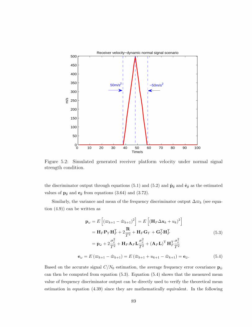
0 10 20 30 40 50 60 70 80 90 1000
50
100
150
200
250
300
350
400
450
500
Time/s
m/s
Receiver velocity−dynamic normal signal scenario
50m/s2 −50m/s2
Figure 5.2: Simulated generated receiver platform velocity under normal signalstrength condition.
the discriminator output through equations (5.1) and (5.2) and pθ and eθ as the estimated
values of pθ and eθ from equations (3.64) and (3.72).
Similarly, the variance and mean of the frequency discriminator output ∆$k (see equa-
tion (4.9)) can be written as
pω = E[($k+1 − $k+1)2
]= E
[(HF∆xk + uk)
2]
= HFPYHTF + 2
R
T 2+ HFGY + GT
YHTF
= pω + 2σ2v
T 2+ HFAFL
σ2v
T 2+ (AFL)T HT
F
σ2v
T 2
(5.3)
eω = E ($k+1 − $k+1) = E ($k+1 + uk+1 − $k+1) = eω. (5.4)
Based on the accurate signal C/N0 estimation, the average frequency error covariance pω
can then be computed from equation (5.3). Equation (5.4) shows that the measured mean
value of frequency discriminator output can be directly used to verify the theoretical mean
estimation in equation (4.39) since they are mathematically equivalent. In the following
89

subsections, we denote pω and eω as the measured values of pω and eω from the frequency
discriminator output through equations (5.3) and (5.4) and pω and eω as the estimated
values of pω and eω from equations (4.33) and (4.39).
5.1.2 Simulation verification
1). Phase tracking loop: The 2-state and 3-state phase tracking loops with LPIF ,
LWF and LKF are tested. The integration time is 1ms, the value of BN for LPIF is set
at 50Hz and the value of qa in 3-state tracking loop is set as 50m2/s5. To validate our
theoretical analysis in a dynamic situation, the measured and theoretical estimated values
of eθ and pθ for these 5 satellites signals are listed in Table 5.1 and Table 5.2.
Table 5.1: Validation of analytic equations (3.64) and (3.72) in 2-state phase trackingloop for various LOS accelerations when C/N0 = 46dB-Hz
PRN/a(m/s2)LPIF (BN = 50Hz, T = 1ms) LWF/LKF (T = 1ms)
Measured/Theoretical Measured/Theoretical Measured/Theoretical Measured/Theoretical
eθ/eθ(◦)
√pθ/√
pθ(◦) eθ/eθ(
◦)√
pθ/√
pθ(◦)
6/ -37.3 -7.9/-7.9 2.6/2.2 –/-59.5 –/1.910/ -48.2 -10.2/-10.2 2.4/2.2 –/-76.9 –/1.912/ -20.9 -4.4/ -4.4 2.6/2.2 -32.9/ -33.5 2.3/1.913/ -4.9 -1.0/ -1.0 2.5/2.2 -7.7/ -7.8 2.1/1.923/ 8.2 1.7/1.7 2.7/2.2 12.8/13.1 2.6/1.9
Note: –represents unavailable measurements due to the loss of lock;
Table 5.2: Validation of analytic equations (3.64) and (3.72) in 3-state phase trackingloop for various LOS accelerations when C/N0 = 46dB-Hz
PRN/a(m/s2)LPIF (BN = 50Hz, T = 1ms) LWF/LKF (qa = 50m2/s5, T = 1ms)
Measured/Theoretical Measured/Theoretical Measured/Theoretical Measured/Theoretical
eθ/eθ(◦)
√pθ/√
pθ(◦) eθ/eθ(
◦)√
pθ/√
pθ(◦)
6/ -37.3 -1.4e-5/0 2.6/2.4 -5.0e-4/0 2.5/2.210/ -48.2 -3.0e-5/0 2.4/2.4 -6.0e-4/0 2.4/2.212/ -20.9 1.9e-5/0 2.6/2.4 -2.3e-3/0 2.5/2.213/ -4.9 1.2e-5/0 2.5/2.4 -1.7e-3/0 2.4/2.223/ 8.2 2.3e-5/0 2.8/2.4 -2.9e-3/0 2.6/2.2
As can be observed in Table 5.1, the LOS accelerations of PRN 12 and PRN 23 are
90

about −20.9m/s2 and 8.2m/s2, and the values of eθ in the 2-state phase tracking loop
with LPIF are −4.4◦ and 1.7◦, respectively. This indicates that a larger magnitude of LOS
acceleration is associated with a larger steady state phase error. It can also be observed
that the values of eθ of PRN 12 and PRN 23 in the tracking loop with LWF /LKF are about
−32.9◦ and 12.8◦, respectively, much larger than that of the PIF-based tracking loop. In
some cases such as PRN 6 and PRN 10, the 2-state phase tracking loop with LWF and
LKF even lost lock due to the large dynamics. That’s because LWF and LKF are designed
with MMSE criterion; the equivalent bandwidth is too narrow to be effective in tracking
the high dynamic signals. Since LPIF is designed with predefined value of BN ; thus, the
loop can handle the dynamic error if BN is sufficiently large (50Hz in this case). However,
the dynamic stress error eθ can be effectively eliminated by the 3-state tracking loop, as
can be seen in Table 5.2. Furthermore, the values of√
pθ are similar for the 3-state and the
2-state cases. As a result, excluding the cases with loss of lock, the measured values, i.e.,
eθ and pθ agree with the estimated values, i.e., eθ and pθ which validates our theoretical
derivations of analytic equations (3.64) and (3.72) in phase tracking loop.
2). Frequency tracking loop: The 1-state and 2-state PIF-based frequency tracking
loops with T = 1ms and BW = 50Hz are tested. To validate our theoretical analysis in a
dynamic situation, the measured and theoretical estimated values of eω and pω for these 5
satellites signals are listed in Table 5.3.
Table 5.3: Validation of analytic equations (4.33) and (4.39) in 1-state and 2-statefrequency tracking loops for various LOS accelerations when C/N0 = 46dB-Hz
PRN/a(m/s2)1-state(BW = 50Hz, T = 1ms) 2-state(BW = 50Hz, T = 1ms)
Measured/Theoretical Measured/Theoretical Measured/Theoretical Measured/Theoretical
eω/eω(Hz)√
pω/√
pω(Hz) eω/eω(Hz)√
pω/√
pω(Hz)6/ -37.3 -20.7/-20.5 5.0/3.8 6.4e-4/0 4.7/2.510/ -48.2 -27.1/-26.5 4.7/3.8 1.6e-3/0 3.8/2.512/ -20.9 -11.7/-11.5 4.8/3.8 -2.7e-5/0 3.7/2.513/ -4.9 -2.7/-2.7 4.2/3.8 -3.8e-4/0 4.6/2.523/ 8.2 4.6/4.5 5.1/3.8 -5.6e-4/0 4.8/2.5
As can be observed in Table 5.3, the values of eω in the 1-state frequency tracking loop
for PRN 12 and PRN 23 satellite signals are −11.7m/s2 and 4.6m/s2, respectively. This
indicates that a larger magnitude of LOS acceleration is associated with a larger steady state
91

frequency error in frequency tracking loop which is similar to phase tracking loop. While,
this dynamic stress error can be effectively eliminated in higher order frequency tracking
loop, such as 2-state frequency tracking loop, where the bias due to receiver dynamics are
estimated. Besides, the values of eω and pω agree with the estimated values, i.e., eω and
pω which validates our theoretical derivations of analytic equations (4.33) and (4.39) in
frequency tracking loop.
5.2 Simulation Results of adaptive phase/frequency
tracking scheme
Two scenarios, the static weak signals and dynamic weak signals, are conducted to verify our
theoretical optimization analysis and to evaluate the performance of the proposed adaptive
phase and frequency tracking loops in the presence of thermal noise, oscillator noise, and
receiver platform dynamics.
1 2 3 4 5 6 7 8 9 10 11 12 13 14 15 16 17 18 19 2015
20
25
30
35
40
45
Time/min
C/N0−weak signal scenario
dB−H
z
−1dB/1min −2dB/1min
Figure 5.3: Simulated generated signal C/N0 under static condition.
92

5.2.1 Static weak signal scenario
In this scenario, the receiver is assumed to be statically located at (N39◦, W82◦). 8 channels
are simulated and the signal C/N0 for these 8 channels are set as 46dB-Hz for two minutes,
then the signal power is decreased 1dB per minute for 6 minutes, then at 2dB per minute
rate until the maximum attenuation of 29dB is reached as shown in Fig.5.3. The RF front-
end with HQO down-converts the input signal to baseband with IF of 0MHz, sampled at
100MHz, and stored with 16-bit resolution for post-processing. Additionally, a NovAtel
receiver was also connected to the simulator to record data simultaneously with the RF
front-end for the purpose of comparison.
600 700 800 900 1000 1100 12000
5
10
15
20
25
30
35
40
Time (s)
C/N
o (d
B−H
z)
(a)
1ms−PIF20ms−PIFadp−PIF1ms−WF/KF20ms−WF/KFadp−WF/KFActual value
Figure 5.4: C/N0 estimations variation in 2-state phase tracking loops for PRN 19satellite signal after 600s (C/N0 < 35dB-Hz). The estimated C/N0 is used to tune Toptand BNopt in adaptive phase tracking loops as well as measurement noise covariancematrix R in WF/KF-based phase tracking loops.
1). Adaptive phase tracking loop scheme: Three different types of 2-states phase
tracking loops are evaluated for static weak signals. They are:
93

600 700 800 900 1000 1100 12000
10
20
30
40
50
60
70
80
90
100
Time (s)
T opt (
ms)
(b)
adp−PIFadp−WF/KFadp−PIF−actual valueadp−WF/KF−actual value
Figure 5.5: The variation of Topt with C/N0 in 2-state adaptive PIF- and WF/KF-based phase tracking loops.
94

600 700 800 900 1000 1100 12000.5
1
1.5
2
2.5
3
Time (s)
BN
opt (
Hz)
(c)
adp−PIFadp−PIF−actua value
Figure 5.6: The variation of BNopt with C/N0 in 2-state adaptive PIF-based phasetracking loop.
95

600 700 800 900 1000 1100 12002550
2600
2650
2700
2750
Time (s)
Dop
pler
freq
uenc
y (H
z)
1ms−PIF20ms−PIFadp−PIF1ms−WF/KF20ms−WF/KFadp−WF/KFActual value
NovAtel lost lock
Figure 5.7: Doppler frequency estimations in the 2-state phase tracking loops for PRN19 satellite signal after 600s (C/N0 < 35dB-Hz) under static weak signal condition.The proposed adaptive phase tracking loops are able to maintain tracking throughoutthis very challenging time period while other phase tracking loops lose lock graduallywhen the signal strength decreases with time.
96
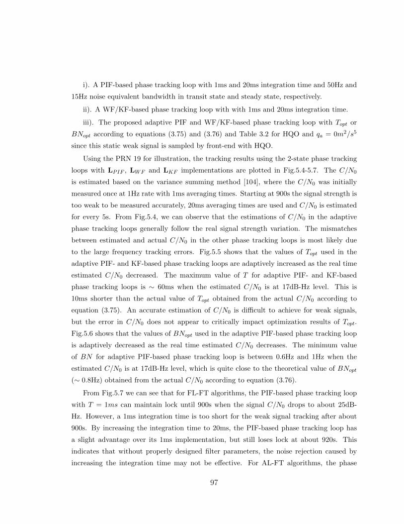
i). A PIF-based phase tracking loop with 1ms and 20ms integration time and 50Hz and
15Hz noise equivalent bandwidth in transit state and steady state, respectively.
ii). A WF/KF-based phase tracking loop with with 1ms and 20ms integration time.
iii). The proposed adaptive PIF and WF/KF-based phase tracking loop with Topt or
BNopt according to equations (3.75) and (3.76) and Table 3.2 for HQO and qa = 0m2/s5
since this static weak signal is sampled by front-end with HQO.
Using the PRN 19 for illustration, the tracking results using the 2-state phase tracking
loops with LPIF , LWF and LKF implementations are plotted in Fig.5.4-5.7. The C/N0
is estimated based on the variance summing method [104], where the C/N0 was initially
measured once at 1Hz rate with 1ms averaging times. Starting at 900s the signal strength is
too weak to be measured accurately, 20ms averaging times are used and C/N0 is estimated
for every 5s. From Fig.5.4, we can observe that the estimations of C/N0 in the adaptive
phase tracking loops generally follow the real signal strength variation. The mismatches
between estimated and actual C/N0 in the other phase tracking loops is most likely due
to the large frequency tracking errors. Fig.5.5 shows that the values of Topt used in the
adaptive PIF- and KF-based phase tracking loops are adaptively increased as the real time
estimated C/N0 decreased. The maximum value of T for adaptive PIF- and KF-based
phase tracking loops is ∼ 60ms when the estimated C/N0 is at 17dB-Hz level. This is
10ms shorter than the actual value of Topt obtained from the actual C/N0 according to
equation (3.75). An accurate estimation of C/N0 is difficult to achieve for weak signals,
but the error in C/N0 does not appear to critically impact optimization results of Topt.
Fig.5.6 shows that the values of BNopt used in the adaptive PIF-based phase tracking loop
is adaptively decreased as the real time estimated C/N0 decreases. The minimum value
of BN for adaptive PIF-based phase tracking loop is between 0.6Hz and 1Hz when the
estimated C/N0 is at 17dB-Hz level, which is quite close to the theoretical value of BNopt
(∼ 0.8Hz) obtained from the actual C/N0 according to equation (3.76).
From Fig.5.7 we can see that for FL-FT algorithms, the PIF-based phase tracking loop
with T = 1ms can maintain lock until 900s when the signal C/N0 drops to about 25dB-
Hz. However, a 1ms integration time is too short for the weak signal tracking after about
900s. By increasing the integration time to 20ms, the PIF-based phase tracking loop has
a slight advantage over its 1ms implementation, but still loses lock at about 920s. This
indicates that without properly designed filter parameters, the noise rejection caused by
increasing the integration time may not be effective. For AL-FT algorithms, the phase
97

tracking loop with WF/KF is slightly better because the loop gain LWF /LKF is adjusted
according to the signal strength. The WF/KF-based phase tracking loops with T = 1ms
and T = 20ms maintain tracking until 920s and 1000s, which are respectively 20s and 80s
longer (2dB better) than that in PIF-based phase tracking loops implementations. The
adaptive PIF/WF/KF-based phase tracking loops improve the tracking sensitivity by at
least 6dB due to their adaptively self-adjusting integration time and gain matrix. An
even longer integration time (>40ms) was invoked in the adaptive phase tracking loops to
maintain tracking of the weak signal until the end of the data sequence when C/N0 reached
the 17dB-Hz level.
The NovAtel receiver lost lock at an attenuation level of -19dB (C/N0 = 27dB-Hz) at
about 840 seconds. The results indicate that the adaptive phase tracking loops outperforms
FL-FT and AL-FT algorithms, validating the state space design and optimization analysis
for generalized phase tracking loop under weak signal condition for a receiver with HQO.
600 700 800 900 1000 1100 1200−5
0
5
10
15
20
25
30
35
40
Time (s)
C/N
o (d
B−H
z)
(a)
1ms−adp10ms−adp1ms−KF10ms−KFActual value
Figure 5.8: C/N0 estimations variation in 1-state frequency tracking loops for PRN19 satellite signal after 600s (C/N0 < 35dB-Hz) under static weak signal condition.The estimated C/N0 is used to tune BWopt in adaptive frequency tracking loops aswell as measurement noise covariance matrix R in KF-based frequency tracking loops.
98

600 700 800 900 1000 1100 12000
0.5
1
1.5
2
2.5
Time (s)
BW
opt (
Hz)
(b)
1ms−adp10ms−adpActual value−1msActual value−10ms
Figure 5.9: The variation of BWopt with C/N0 in adaptive PIF-based frequency track-ing loop.
99

600 700 800 900 1000 1100 12002550
2600
2650
2700
2750
Time (s)
Dop
pler
freq
uenc
y (H
z)
(c)
1ms−adp10ms−adp1ms−KF10ms−KFActual value
Figure 5.10: Doppler frequency estimations in 1-state frequency tracking loops forPRN 19 satellite signal after 600s (C/N0 < 35dB-Hz) under static weak signal condi-tion. The optimized frequency tracking loops are better than the KF-based frequencytracking loops for both T = 1ms and 10ms.
100

2). Adaptive frequency tracking loop scheme: The 1-state adaptive frequency
tracking loops with T = 1ms and 10ms and the corresponding value of BWopt are adopted
to process this static weak signal. The KF-based frequency tracking loops with T = 1ms
and 10ms in [30] are also shown in the figure. Note that the KF-based frequency tracking
loop does not take into consideration of the non-white noise characteristics of frequency
estimation noise. It is shown here for comparison purposes.
Using the PRN 19 for illustration, Fig.5.8 shows that the estimations of C/N0 with
T = 10ms follow the real signal strength trend more accurately than other approaches,
especially when the signal strength is low. Fig.5.9 shows that BWopt for both T = 1ms and
10ms adaptively decreases as C/N0 decreases, with BWopt being slighter lower for T = 1ms
than for 10ms especially when the signal is weak. Fig.5.10 shows that as signal strength
decreases, the frequency error increases. This trend is particularly obvious for T = 1ms
after about 700 seconds (C/N0=33dB-Hz) in the KF-based frequency tracking loop and
1000 seconds (C/N0=23dB-Hz) in the adaptive PIF-based frequency tracking loop. This is
in disagreement with the theoretical analysis in Table 4.1 which shows that the adaptive
frequency tracking loop could track a weak signal as low as 0dB-Hz. This disagreement can
be attributed to errors in the assumption C/N0 estimation. The maximum frequency error
in the 1ms frequency tracking loop can be as much as 42Hz as compared to the frequency
error threshold. In the real implementation, this large frequency error degrades the C/N0
estimations. To improve the tracking accuracy and to reduce C/N0 estimation errors when
the signal is weak, longer integration times such as T = 10ms should be used. Using
T = 10ms, the KF-based frequency tracking loop lost lock at 1000 seconds (C/N0=23dB-
Hz), while the adaptive PIF-based frequency tracking loop maintains tracking through out
the time period. The theoretical analysis is based on the rules that 3-sigma frequency jitter
should be less than one-forth of the frequency pull-in range of the frequency discriminator.
It indeed shows that the theoretical tracking sensitivity is close to 0dB-Hz. However, in the
real implementation, the large frequency error degrades the I and Q accumulation energy
which affects both the C/N0 estimation and frequency error measurement. Simulation
results show that the frequency tracking results deviate from the theoretical prediction,
suggesting that more research is required to bridge the gap.
The better performance of the adaptive PIF-based frequency tracking loop over KF-
based frequency tracking loop validates the state space design and optimization analysis for
generalized FLL under the static and weak signal condition for a receiver front-end with
101

HQO. Comparing Fig.5.10 to Fig.5.7, the adaptive frequency tracking loop with T = 10ms is
equivalent to the adaptive PIF-based phase tracking loop with a maximum 60ms integration
time and better than the KF-based phase tracking loop with T = 20ms. It shows that even
with shorter integration time, a well-designed frequency tracking loop is superior to or at
least equivalent to a well-designed phase tracking loop in weak signal processing.
5.2.2 dynamic weak signal scenario
In this simulation, signal attenuation and dynamics are applied simultaneously, as can be
seen in Fig.5.11. For signal attenuation, the signal power starts at the nominal 46dB-Hz
level and was decreased by 1dB per 5s starting at 20s. The maximum attenuation reaches
20dB at t = 120s and maintained at this level for 60s, followed by a recovery period with
1dB per 5s until it reaches back to the nominal level. For signal dynamics simulation, the
receiver is static in the first 20s, then it starts moving to the east with an acceleration of
50m/s2 for 100s. When t = 120s, the acceleration is at zero with a negative jerk of 50m/s3.
After this, the receiver remains at a constant velocity until t = 180s, then it slows down
with negative acceleration for 100s and stops at t = 280s. The RF front-end with LQO
collects the data with an IF at 4.309MHz, sampling frequency at 12MHz, and stored in
1-bit resolution for post-processing. Note that this scenario may not be very common in
practice, we just want to use to this profile to have a preliminary verification of our adaptive
tracking loop performance when the weak signal and high dynamic coincide. The further
real data test will be conducted in future.
1). Adaptive phase tracking loop scheme: Three types of 3-states phase tracking
loops are evaluated for dynamic weak signal processing. They are:
i). A PIF-based phase tracking loop with 1ms and 20ms integration times. A 50Hz
noise equivalent bandwidth is used in both the transit- and steady-state respectively.
ii). A WF/KF-based phase tracking loop with 1ms and 20ms integration times and
corresponding qa values for the dynamic scenarios described above and estimated using
equation (3.12).
iii). The proposed adaptive PIF and WF/KF-based phase tracking loop with Topt or
BNopt computed according to equations (3.75) and (3.76) and Table 3.2 for the case of
qa = 10m2/s5 and a receiver with LQO.
102

0 50 100 150 200 250 30025
30
35
40
45
Time(s)
(a)
C/N
o(dB
−Hz)
0 50 100 150 200 250 3000
2000
4000
6000
(b)
Vel
ocity
(m/s
)
Time(s)
jM
=50m/s3
−1dB/5s keep +1dB/5s
Figure 5.11: The signal C/N0 and platform velocity in dynamic weak signal scenario.(a). The variation of signal C/N0; (b). The variation of platform dynamics withmaximum jerk of ±50m/s3.
Fig.5.12 shows that the estimated C/N0 in all three adaptive phase tracking loops in
general follows the real signal strength variations. The mismatch between estimated and
real C/N0 in all non-adaptive phase tracking loops is most likely due to the large frequency
tracking errors.
Fig.5.13 and 5.14 show that the values of Topt and BNopt in the adaptive phase tracking
loops are automatically tuned according to C/N0 estimations, although there are some
discrepancies between the theoretically computed Topt and the actual Topt according to
equations (3.75) and (3.76) adopted by the tuning process. For example, the theoretical
Topt is 7ms and 8ms for the PIF- and WF-based adaptive phase tracking loops respectively
when C/N0 is 26dB-Hz. In the real implementation, Topt is at about 10ms due to an
inaccurate C/N0 estimation when the signal is weak. Fig.5.13 shows that the minimum
value of BN for adaptive PIF-based phase tracking loop is between 11Hz and 15Hz in real
implementations, which is quite close to the theoretical value of BNopt (∼ 12Hz) obtained
based on the actual C/N0. Hence, the error in the C/N0 estimation does not appear to
103

0 50 100 150 200 250 3005
10
15
20
25
30
35
40
45
50
Time (s)
C/N
o(dB
−Hz)
1ms−PIF20ms−PIFadp−PIF1ms−WF/KF20ms−WF/KFadp−WF/KFActual value
Figure 5.12: C/N0 estimations variation in 3-state phase tracking loops for PRN 14satellite signal under dynamic weak signal condition. The estimated C/N0 is used totune Topt and BNopt in adaptive phase tracking loops as well as measurement noisecovariance matrix R in WF/KF-based phase tracking loops.
104

0 50 100 150 200 250 3000
5
10
15
Time (s)
T opt (
ms)
adp−PIFadp−WF/KFadp−PIF−actual valueadp−WF/KF−actual value
Figure 5.13: The variation of Topt with signal C/N0 in 3-state adaptive PIF- andWF/KF-based phase tracking loops.
105

0 50 100 150 200 250 30010
15
20
25
30
35
Time (s)
BN
opt (
Hz)
adp−PIFadp−PIF−actual value
Figure 5.14: The variation of BNopt with signal C/N0 in 3-state adaptive PIF-basedphase tracking loop.
106

0 50 100 150 200 250 3000
0.2
0.4
0.6
0.8
1
1.2
1.4
1.6
1.8
2x 10⁴
Time (s)
Dop
pler
freq
uenc
y (H
z)
1ms−PIF20ms−PIFadp−PIF1ms−WF/KF20ms−WF/KFadp−WF/KFActual value
Figure 5.15: Doppler frequency estimations in 3-state phase tracking loops for PRN14 satellite signal under dynamic weak signal condition. Only the proposed adaptivephase tracking loops are able to maintain tracking while others have lost lock.
107

0 50 100 150 200 250 300−300
−200
−100
0
100
200
300
Time (s)
Dop
pler
freq
uenc
y ra
te (
Hz/
s)
1ms−PIF20ms−PIFadp−PIF1ms−WF/KF20ms−WF/KFadp−WF/KFActual value
Figure 5.16: Doppler frequency rate estimations in 3-state phase tracking loops forPRN 14 satellite signal under dynamic weak signal condition. Only the Dopplerfrequency rate estimations in the proposed adaptive phase tracking loops the generallyfollow the signal dynamic, while others have diverged after 120s.
108

critically impact the optimization results for Topt and BNopt.
Fig.5.15 shows the Doppler frequency estimations of the 3-state phase tracking loops,
where the maximum changes of Doppler frequency are about 15000Hz during acceleration
from 20s to 120s and -14000Hz during deceleration from 180s to 280s. A loss-of-lock occurs
in the PIF-based PLL with T = 1ms at about 110s. Using a longer time integration, such
as T = 20ms enables the PIF-based phase tracking loop to maintain lock for 10s longer
(2dB better). The WF/KF-based phase tracking loop with a variable gain demonstrates
improved performance. For example, for T = 1ms, the WF/KF-based phase tracking loop
is about 2dB better than the PIF-based phase tracking loop in tracking sensitivity. This
observation shows that WF/KF has the potential to achieve better noise performance due
to its narrow equivalent noise bandwidth than the model-free approach PIF. However, the
same conclusion doesn’t hold any more when jerk starts at 120s. The WF/KF-based phase
tracking loop with T = 20ms loses lock almost at the same time with 20ms PIF-based
phase tracking loop. Since as C/N0 decreases, the noise equivalent bandwidth in WF/KF-
based phase tracking loop decreases. Hence, the narrower noise equivalent bandwidth in
WF/KF degrades the dynamic adaptability when dynamic stress occurs. Moreover, longer
integration time, such as T = 20ms even makes worse in dynamic signal tracking.
Fig.5.16 shows the estimated Doppler rate. It can be seen that the Doppler rate estima-
tions are consistent with the actual rates for the adaptive schemes, while the estimations
from non-adaptive approaches deviate from the true values at different times. The adaptive
schemes also accurately estimated the receiver’s jerks at 20s, 120s, 180s and 280s.
The superior performance of the adaptive phase tracking loops over FL-FT algorithm
and AL-FT algorithm validates the state space design and optimization analysis for gener-
alized phase tracking loop for dynamic weak signals using a receiver with LQO.
2). Adaptive frequency tracking loop scheme: The 2-state adaptive frequency
tracking loops with T = 1ms and 10ms are adopted to process this dynamic weak signal.
KF-based frequency tracking loops with T = 1ms and 10ms are also tested for the perfor-
mance comparison purposes. The values of qa are set as 1m2/s5 and 10m2/s5 to represent
signal dynamics described by equation (3.12) for T = 1ms and 10ms, respectively.
Fig.5.17 shows that the estimations of C/N0 in the adaptive frequency tracking loops
generally follow the real signal strength variation. The mismatch between the estimated and
real C/N0 in the KF-based frequency tracking loops is most likely due to the large frequency
109
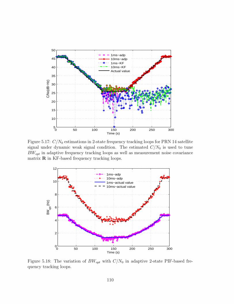
0 50 100 150 200 250 3005
10
15
20
25
30
35
40
45
50
Time (s)
C/N
o(dB
−Hz)
1ms−adp10ms−adp1ms−KF10ms−KFActual value
Figure 5.17: C/N0 estimations in 2-state frequency tracking loops for PRN 14 satellitesignal under dynamic weak signal condition. The estimated C/N0 is used to tuneBWopt in adaptive frequency tracking loops as well as measurement noise covariancematrix R in KF-based frequency tracking loops.
0 50 100 150 200 250 3000
2
4
6
8
10
12
Time (s)
BW
opt (H
z)
1ms−adp10ms−adp1ms−actual value10ms−actual value
Figure 5.18: The variation of BWopt with C/N0 in adaptive 2-state PIF-based fre-quency tracking loops.
110

0 50 100 150 200 250 300
0
2000
4000
6000
8000
10000
12000
14000
16000
18000
20000
Time (s)
Dop
pler
freq
uenc
y (H
z)
1ms−adp10ms−adp1ms−KF10ms−KFActual value
Figure 5.19: Doppler frequency estimations in 2-state frequency tracking loops forPRN 14 satellite signal under dynamic weak signal condition. Only the proposedadaptive frequency tracking loops are able to maintain tracking while KF-based fre-quency tracking loops with T = 1ms and 10ms respectively lost of lock after 120sand 180s.
111

0 50 100 150 200 250 300−300
−200
−100
0
100
200
300
Time (s)
Dop
pler
freq
uenc
y ra
te (
Hz/
s)
1ms−adp10ms−adp1ms−KF10ms−KFActual value
Figure 5.20: Doppler frequency rate estimations in 2-state frequency tracking loopsfor PRN 14 satellite signal under dynamic weak signal condition. Only the Dopplerfrequency rate estimations in the proposed adaptive frequency tracking loops thegenerally follow the signal dynamic while KF-based frequency tracking loops withT = 1ms and 10ms respectively diverge after 120s and 180s.
112

tracking errors. Fig.5.18 shows that the values of BWopt used in the adaptive frequency
tracking loops are automatically tuned according to the real time C/N0 estimations, and
these values generally follow the theoretical values that obtained for the actual C/N0. Again,
BWopt with T = 1ms is smaller than that with T = 10ms. Fig.5.19 shows the KF-
based frequency tracking loops with T = 1ms and 10ms lost lock at about 120s and 180s,
respectively, while the adaptive frequency tracking loops maintain tracking throughout the
time period. However, there are some frequency errors when T = 1ms due to the inaccurate
measurements when the signal is weak from 120s to 180s. Fig. 5.20 shows that the Doppler
frequency rate estimations in the KF-based frequency tracking loops with T = 1ms and
10ms deviate from the truth after 120s and 200s, respectively. The estimations in the
adaptive PIF-based frequency tracking loop with T = 1ms follows the signal dynamics in
general, but with some disturbance from 80s to 220s when C/N0 drops to 26dB-Hz. A
frequency tracking loop with short integration time may be adequate to satisfy the weak
and dynamic signal tracking requirement, but may be at the risk of having a lower tracking
accuracy. With a longer integration time, such as T = 10ms, the estimations in the adaptive
frequency tracking loop are more accurate throughout the time period.
The above results show that the adaptive frequency tracking loop perform better than
the KF-based frequency tracking loop for dynamic weak signals using a receiver front end
with a LQO. Comparing the Doppler frequency and frequency rate estimations in adaptive
PIF-based phase tracking loop in Fig. 5.15-5.16 with that in adaptive PIF-based frequency
tracking loop in Fig. 5.19-5.20 for C/N0 = 26dB-Hz shows that the 2-state PIF-based fre-
quency tracking loop with T = 10ms and BWopt at about 4Hz achieves equivalent tracking
performance to that of the 3-state PIF-based phase tracking loop with BNopt at about 12Hz
and Topt at 10ms . Both tracking loops perform better than the 2-state PIF-based frequency
tracking loop with T = 1ms and BWopt at about 1.8Hz.
113
Chapter 6
Conclusions and Future Work
6.1 Conclusion
In this thesis, we established a generalized carrier tracking loop architecture from a control
system perspective. A state space model and state feedback/state estimator design approach
for general carrier tracking loop problem were studied. Two generalized carrier tracking
loops, namely, the generalized phase tracking loop and the generalized frequency tracking
loop, were designed, analyzed, and optimized.
In generalized phase tracking loop design, three traditional filter design methods, i.e.,
PIF, WF, and KF were presented and unified within the state space framework. The rela-
tionships between their corresponding state estimator gain matrices and parameters, such
as the integration time, the loop bandwidth, dynamic parameter, and the oscillator h-
parameters, were derived. Our analysis demonstrated the well-known fact that WF and KF
designs are equivalent under the assumption of white Gaussian noise in the time-invariant
linear systems, i.e., the WF state estimator gain is an exact closed form expression for the
steady-state KF gain. Based on the MMSE criteria, the phase tracking loop with PIF,
WF, and KF were optimized to improve the tracking sensitivity and dynamic responses.
For the convenience of actual implementations, the relationships between the optimal in-
tegration time, Topt and C/N0, the optimal phase tracking loop bandwidth, BNopt, and
C/N0 for different dynamics and oscillator qualities were provided to facilitate the phase
tracking loop design. The phase tracking sensitivity limits of these tracking loops were
obtained in terms of the 3-sigma rule. We demonstrated that if a 2-state model is used in
114

static environment, the optimized PIF, WF, and KF can be tuned to achieve comparable
performance. The maximum tracking sensitivity is limited by the oscillator quality, where
the tracking sensitivity limits of the receivers with HQO are as much as 6dB-Hz in pilot
channel and 13dB-Hz in data channel, respectively, which are 9dB higher than that of the
receivers with LQO. If a 3-state model is used in dynamic environment, the optimized WF
and KF are equivalent and slightly better than the optimized PIF. We analytically demon-
strated that the tracking sensitivity deteriorates as the platform dynamic increases. These
results demonstrated that under the uniform optimization criteria, the phase tracking loop
performance is mainly limited by the oscillator quality and platform dynamics, regardless
of PIF, WF, or KF design approaches.
In generalized frequency tracking loop design, taking the non-white noise characteristic
into account, the PIF design was formulated in the state space framework. Performance
metrics, such as frequency tracking error variance and dynamic stress error, were derived
to evaluate the performance of frequency tracking loop designs under the effects of thermal
noise, oscillator noise, and platform dynamics. Relationships between the optimal frequency
tracking loop bandwidth, BWopt, and C/N0 for different dynamics and integration time were
provided to facilitate the frequency tracking loop design. Based on the MMSE criteria,
the frequency tracking loop with PIF was optimized to improve the frequency tracking
performance. Theoretical analysis showed that the oscillator noise has a minor effect on
frequency tracking loop performance and the frequency tracking loop has at least 6dB
improvement in tracking sensitivity compared to the phase tracking loop with the same
signal dynamics.
Following this theoretical analysis, an adaptive phase tracking scheme and also an adap-
tive frequency tracking scheme to track weak and high dynamic signals were proposed. Two
case studies using simulator to generate signals with high receiver platform dynamics and
low signal power were conducted to verify the theoretical analysis, as well as the adaptive
tracking schemes. The simulation results confirmed that: (1) the adaptive phase track-
ing scheme is superior to the traditional PLL; (2) the adaptive frequency tracking scheme
is superior to the traditional KF-based FLL; (3) the 1-state adaptive frequency tracking
loop with a 10ms integration time achieves almost equivalent tracking performance with
the 2-state adaptive phase tracking loop with adaptive integration time (60ms maximum)
for C/N0 as low as 17dB-Hz under the static scenario; (4) the 2-state adaptive frequency
tracking loop with a 10ms integration time and BWopt at about 4Hz achieves an equivalent
115

tracking performance to that of the 3-state PIF-based phase tracking loop with BNopt at
about 12Hz and Topt at 10ms. Both tracking loops perform better than the 2-state PIF-
based frequency tracking loop with T = 1ms and BWopt at about ∼1.8Hz for C/N0 as
low as 26dB-Hz under a maximum 50m/s3 jerk dynamic condition. These results validate
the effectiveness of optimized loop parameters selection and demonstrate that the adap-
tive phase tracking and the adaptive frequency tracking schemes can enhance the tracking
performance in challenging environments with weak signal and/or dynamic receiver motion.
6.2 Future Work
A number of open questions and unresolved issues, have been identified and further research
are suggested here.
1. The performance of the proposed adaptive carrier tracking algorithm depends on
good signal C/N0 estimation. However, in the presence of multipath fading or inter-
ference, the C/N0 estimation may be affected by large signal level fluctuations due to
constructive interference. The adaptive filter weighs these unreliable estimates more
strongly due to the high C/N0 and the tracking loop quickly can become unstable.
Therefore, to improve the carrier tracking robustness and reliability, robust C/N0
estimation methodology and improved carrier tracking algorithms to mitigate inter-
ference and multipath effects need to be further investigated. Additionally, the C/N0
estimator is derived under the assumptions of perfect frequency synchronization, data
bit aiding and constant signal phase during the observation window. However, in the
frequency tracking loop, larger frequency errors may degrade the C/N0 estimator ac-
curacy which finally deteriorate the tracking performance. A sensitivity experiment
that shows how C/N0 is affected by frequency error is required.
2. The state feedback design analysis in Chapter 3 shows that when B is chosen as
[0; 1] or [1; 1], the control plant effectively corresponds to a single-input NCO, i.e.,
the rate-only feedback NCO or the phase and rate feedback NCO in traditional PLL
design. Furthermore, the state space design framework also enables the multi-input
NCO operation, such as B = I. The selection of B = I and K = A simplifies the
error state estimation and enables us to cast the traditional PLL design to the state
space framework. However, from control system design perspective, other possible
116

B and K selections that ensure system controllability and stability can be adopted
as well in order to satisfy the specific system performance, such as robustness. The
different B and K selections need to be studied to improve the tracking loop design.
3. The state estimator design analysis in Chapter 3 and Chapter 4 shows that the
corresponding state estimator gain matrices are obtained by casting the traditional
single-input single-output tracking loop designs, such as PIF- and WF-based PLL
and PIF-based FLL, to the state space tracking architecture. It is known that the
state space framework is more general and enables the multiple-input multiple-output
control system design. Hence, many other filter techniques and estimation approach-
es, such as LSE [32] and MHE [98] based on the multiple phase error or frequency
error measurements, could be used to design the state estimator. Additionally, the
combination of the phase and frequency tracking loop, which is known as FLL-assist-
PLL, could be designed by using the modelling, design, and optimization techniques
presented in this thesis to improve the carrier tracking ability.
4. Optimization analysis in Chapter 3 and Chapter 4 shows that different design ap-
proaches can be unified, evaluated, and compared within the general state space
framework. The optimized performances in these tracking loops are equivalent and
the tracking limits of carrier tracking loop design is ultimately determined by sig-
nal models. Accurate model is key to improve the tracking performance of tracking
loops. This thesis only considers the simplest case that the measurement noise is
white Gaussian noise and assumed to be uncorrelated with the system noise, such as
oscillator noise and dynamics. However, the time-correlated clock errors [103] which
represent the correlation between measurement noise and process noise, will affect the
system performance particularly for longer integration times. Besides, there are var-
ious error sources, such as interference [101] and ionospheric scintillation [102], that
corrupt and distort carrier measurements in real world applications. In the dynamic
scenario, the dynamic stress (g-sensitive) errors or platform vibration-induced errors
also have significant influence on the carrier signal. These errors should be considered
in the signal models in order to improve the carrier tracking performance.
117

List of Publications
[1] R. Yang, K. V. Ling, E. K. Poh, and Y. Morton, “Generalized GNSS Signal Car-
rier Tracking: Part I: Modelling and Analysis,” accepted by IEEE Transactions on
Aerospace and Electronic Systems, January, 2017.
[2] R. Yang, Y. Morton, K. V. Ling, and E. K. Poh, “Generalized GNSS Signal Carrier
Tracking: Part II: Optimization and Implementation,” accepted by IEEE Transac-
tions on Aerospace and Electronic Systems, January, 2017.
[3] R. Yang, Y. Wang, L. Cong, K. V. Ling, and E. K. Poh. “Integration Time Anal-
ysis for High Sensitivity Kalman Filter Based Tracking Loop,” 2015 Pacific PNT,
Honolulu, Hawaii, April 2015.
[4] R. Yang, K. V. Ling, and E. K. Poh. “NCO Models for Tracking Loop Design in
GNSS Software Receiver,” 2014 IEEE/ION PLANS, Monterey, California, May 2014.
[5] R. Yang, K. V. Ling, and E. K. Poh. “Optimal combination of coherent and non-
coherent acquisition of weak GNSS signals,” 2013 Pacific PNT, Honolulu, Hawaii,
April 2013.
[6] Y. Wang, R. Yang, K. V. Ling, and E. K. Poh, “Robust Vector Tracking Loop Using
Moving Horizon Estimation,” , 2015 Pacific PNT, Honolulu, Hawaii, April 2015.
118

Bibliography
[1] William C Stone. Electromagnetic signal attenuation in construction materials. US
Department of Commerce, National Institute of Standards and Technology, Building
and Fire Research Laboratory, 1997.
[2] Gonzalo Seco-Granados, Jose A Lopez-Salcedo, David Jimenez-Banos, and Gustavo
Lopez-Risueno. Challenges in indoor global navigation satellite systems: Unveiling its
core features in signal processing. Signal Processing Magazine, IEEE, 29(2):108–131,
2012.
[3] James T Curran, Gerard Lachapelle, and Colin C Murphy. Improving the design of
frequency lock loops for GNSS receivers. Aerospace and Electronic Systems, IEEE
Transactions on, 48(1):850–868, 2012.
[4] Cillian ODriscoll, Mark G Petovello, and Gerard Lachapelle. Choosing the coherent
integration time for Kalman filter-based carrier-phase tracking of GNSS signals. GPS
solutions, 15(4):345–356, 2011.
[5] Phillip W Ward. Performance comparisons between FLL, PLL and a novel FLL-
assisted-PLL carrier tracking loop under RF interference conditions. In Proceedings
of the 11th International Technical Meeting of the Satellite Division of The Institute
of Navigation (ION GPS 1998), pages 783–795, 1998.
[6] Pratap Misra and Per Enge. Global Positioning System: Signals, Measurements and
Performance Second Edition. Lincoln, MA: Ganga-Jamuna Press, 2006.
[7] Daniele Borio. A statistical theory for GNSS signal acquisition. 2008.
[8] Elliott D Kaplan and Christopher J Hegarty. Understanding GPS: principles and
applications. Artech house, 2005.
119

[9] James Bao-Yen Tsui. Fundamentals of Global Positioning System Receivers: A Soft-
ware Approach, Second Edition. John Wiley and Sons Ltd, 2005.
[10] Cillian O’Driscoll. Performance analysis of the parallel acquisition of weak GPS sig-
nals. PhD thesis, 2007.
[11] Fabio Dovis, Gerard Lachapelle, Daniele Borio, and Anna Martinetti. Comparison of
standard and generalized post-correlation differentially coherent detection strategies
for weak GNSS signal acquisition. Master’s thesis, 2009.
[12] Shashank Satyanarayana. GNSS channel characterization and enhanced weak signal
processing. PhD thesis, University of Calgary, 2011.
[13] Tian Jin, Fangyao Lu, Yang Liu, Honglei Qin, and Xiling Luo. Double differentially
coherent pseudorandom noise code acquisition method for code-division multipleac-
cess system. Signal Processing, IET, 7(7):587–597, 2013.
[14] Feng Xu and Yang Gao. A new GNSS acquisition method with signal down sampling
in frequency domain. In Vehicular Technology Conference, 2009. VTC Spring 2009.
IEEE 69th, pages 1–5. IEEE, 2009.
[15] Rong Yang, Keck Voon Ling, and Eng Kee Poh. Optimal combination of coherent and
non-coherent acquisition of weak GNSS signals. In Pacific PNT, Honolulu, Hawaii,
USA, April 2013. ION.
[16] James T Curran. Weak signal digital GNSS tracking algorithms. PhD thesis, National
University of Ireland, 2010.
[17] Bradford W Parkinson and James J Spilker. Global Positioning System: Theory and
Applications (volume One), volume 1. Aiaa, 1996.
[18] JAMES T Curran, GERARD Lachapelle, and COLIN C Murphy. Digital GNSS PLL
design conditioned on thermal and oscillator phase noise. Aerospace and Electronic
Systems, IEEE Transactions on, 49(1):687–687, 2013.
[19] Alireza Razavi, Demoz Gebre-Egziabher, and Dennis M Akos. Carrier loop archi-
tectures for tracking weak GPS signals. Aerospace and Electronic Systems, IEEE
Transactions on, 44(2):697–710, 2008.
120
[20] Pejman Lotfali Kazemi. Development of new filter and tracking schemes for weak
GPS signal tracking. PhD thesis, University of Calgary, 2010.
[21] Tian Jin and JunXing Ren. Stability analysis of GPS carrier tracking loops by phase
margin approach. GPS solutions, 17(3):423–431, 2013.
[22] Weihua Zhuang. Composite GPS receiver modelling, simulations and applications.
PhD thesis, University of New Brunswick, 1993.
[23] SA Stephens and JB Thomas. Controlled-root formulation for digital phase-locked
loops. Aerospace and Electronic Systems, IEEE Transactions on, 31(1):78–95, 1995.
[24] JB Thomas. An analysis of digital phase-locked loops. 1989.
[25] Jose A Lopez-Salcedo, Del Peral-Rosado, Gonzalo Seco-Granados, et al. Survey on
robust carrier tracking techniques. Communications Surveys and Tutorials, IEEE,
16(2):670–688, 2014.
[26] Weihua Zhuang. Performance analysis of GPS carrier phase observable. Aerospace
and Electronic Systems, IEEE Transactions on, 32(2):754–767, 1996.
[27] Daniele Borio and Gerard Lachapelle. A non-coherent architecture for GNSS digital
tracking loops. annals of telecommunications-annales des telecommunications, 64(9-
10):601–614, 2009.
[28] Daniele Borio, Nadezda Sokolova, and Gerard Lachapelle. Memory discriminators
for non-coherent integration in GNSS tracking loops. In Proc. European Navigation
Conf. ENC, volume 9, 2009.
[29] Cillian ODriscoll and Gerard Lachapelle. Comparison of traditional and Kalman filter
based tracking architectures. In Proceedings of European navigation conference, pages
3–6, 2009.
[30] Jong-Hoon Won, Dominik Dotterbock, and Bernd Eissfeller. Performance comparison
of different forms of Kalman filter approaches for a vector-based GNSS signal tracking
loop. Navigation, 57(3):185–199, 2010.
[31] Jong-Hoon Won, Thomas Pany, and Bernd Eissfeller. Characteristics of Kalman filters
for GNSS signal tracking loop. Aerospace and Electronic Systems, IEEE Transactions
on, 48(4):3671–3681, 2012.
121

[32] Brian DO Anderson and John B Moore. Optimal filtering. Courier Dover Publications,
2012.
[33] Pejman L Kazemi. Optimum digital filters for GNSS tracking loops. In Proceedings of
international technical meeting of the Satellite Division of the Institute of Navigation
(ION GNSS), Savannah, GA, pages 16–19, 2008.
[34] Del Peral-Rosado, Jose A Lopez-Salcedo, Gonzalo Seco-Granados, Jose M Lopez-
Almansa, Joaquın Cosmen, et al. Kalman filter-based architecture for robust and
high-sensitivity tracking in GNSS receivers. In Satellite Navigation Technologies and
European Workshop on GNSS Signals and Signal Processing (NAVITEC), 2010 5th
ESA Workshop on, pages 1–8. IEEE, 2010.
[35] Xinhua Tang, Gianluca Falco, Emanuela Falletti, and Letizia Lo Presti. Practical im-
plementation and performance assessment of an extended Kalman filter-based signal
tracking loop. In Localization and GNSS (ICL-GNSS), 2013 International Conference
on, pages 1–6. IEEE, 2013.
[36] Nesreen I Ziedan. GNSS receivers for weak signals. Artech house, 2006.
[37] Mark L Psiaki and Hee Jung. Extended kalman filter methods for tracking weak GPS
signals. In ION GPS 2002: 15 th International Technical Meeting of the Satellite
Division of The Institute of Navigation, 2002.
[38] Ping Lian, Gerard Lachapelle, and ChangLin Ma. Improving tracking performance
of PLL in high dynamics applications. In ION NTM, volume 1, pages 042–1, 2005.
[39] Kwang-Hoon Kim, Gyu-In Jee, and Jong-Hwa Song. Carrier tracking loop using the
adaptive two-stage Kalman filter for high dynamic situations. International Journal
of Control Automation and Systems, 6(6):948–953, 2008.
[40] Guo Yao, Wu Wenqi, and He Xiaofeng. High dynamic carrier phase tracking based
on adaptive Kalman filtering. In Control and Decision Conference (CCDC), 2011
Chinese, pages 1245–1249. IEEE, 2011.
122
[41] Pedro A Roncagliolo, Cristian E De Blasis, and Carlos H Muravchik. GPS digital
tracking loops design for high dynamic launching vehicles. In Spread Spectrum Tech-
niques and Applications, 2006 IEEE Ninth International Symposium on, pages 41–45.
IEEE, 2006.
[42] Pedro A Roncagliolo, Javier G Garcia, and Carlos H Muravchik. A joint carrier and
data estimation scheme for real-time high dynamics GNSS receivers. In Advanced
satellite multimedia systems conference (asma) and the 11th signal processing for
space communications workshop (spsc), 2010 5th, pages 361–368. IEEE, 2010.
[43] S Han, W Wang, X Chen, and W Meng. Design and capability analyze of high dynamic
carrier tracking loop based on UKF. In Proceedings of the 23rd International Technical
Meeting of The Satellite Division of the Institute of Navigation (ION GNSS 2010),
pages 1960–1966, 2010.
[44] Nesreen I Ziedan and James L Garrison. Extended kalman filter-based tracking of
weak GPS signals under high dynamic conditions. In Proceedings of ION GNSS,
volume 2004, pages 20–31. Citeseer, 2004.
[45] Xinlong Wang, Xinchun Ji, Shaojun Feng, and Vincent Calmettes. A high-sensitivity
GPS receiver carrier-tracking loop design for high-dynamic applications. GPS Solu-
tions, 19(2):225–236, 2015.
[46] S Skone, G Lachapelle, D Yao, W Yu, and R Watson. Investigating the impact of
ionospheric scintillation using a GPS software receiver. In 18th Int. Tech. Meeting of
the Satellite Division of the US Institute of Navigation, pages 1126–1137, 2005.
[47] Faisal A Khan, Andrew G Dempster, and Chris Rizos. Projected bandwidth loop-
an alternative to adaptive bandwidth loops with reduced complexity. In Position
Location and Navigation Symposium (PLANS), 2010 IEEE/ION, pages 1147–1153.
IEEE, 2010.
[48] Mario Gomez Arias. Adaptive Kalman Filter-Based Phase-Tracking in GNSS. BSc
thesis, Technische Universitat Munchen, 2010.
[49] Jong-Hoon Won and Bernd Eissfeller. A tuning method based on signal-to-noise
power ratio for adaptive PLL and its relationship with equivalent noise bandwidth.
IEEE communications letters, 17(2):393–396, 2013.
123

[50] Gerd Ascheid and Heinrich Meyr. Cycle slips in phase-locked loops: A tutorial survey.
Communications, IEEE Transactions on, 30(10):2228–2241, 1982.
[51] James T Curran, Gerard Lachapelle, and Colin C Murphy. An SNR dependent model
for the CDMA FLL. IEEE Transactions on Signal Processing, 60(3):1522–1527, 2012.
[52] Thomas Pany. Navigation signal processing for GNSS software receivers. Artech
House, 2010.
[53] Zhe He. High-Sensitivity GNSS Doppler and Velocity Estimation for Indoor Naviga-
tion. PhD thesis, University of Calgary, 2013.
[54] Daniele Borio, Laura Camoriano, Letizia Lo Presti, and Maurizio Fantino. DTFT-
based frequency lock loop for GNSS applications. IEEE transactions on aerospace
and electronic systems, 44(2):595–612, 2008.
[55] Jong-Hoon Won, Thomas Pany, and Bernd Eissfeller. Iterative maximum likelihood
estimators for high-dynamic GNSS signal tracking. Aerospace and Electronic Systems,
IEEE Transactions on, 48(4):2875–2893, 2012.
[56] S Hinedi. An extended Kalman filter based automatic frequency control loop. 1988.
[57] Victor A Vilnrotter, Sami Hinedi, and Rajendra Kumar. Frequency estimation tech-
niques for high dynamic trajectories. Aerospace and Electronic Systems, IEEE Trans-
actions on, 25(4):559–577, 1989.
[58] Jong-Hoon Won, Thomas Pany, and Bernd Eissfeller. Noniterative filter-based max-
imum likelihood estimators for GNSS signal tracking. Aerospace and Electronic Sys-
tems, IEEE Transactions on, 48(2):1100–1114, 2012.
[59] Pedro A Roncagliolo and Javier G Garcia. High dynamics and false lock resistant
GNSS carrier tracking loops. In Proceedings of The 20th International Technical
Meeting of The Satellite Division of The Institute of Navigation, ION GNSS 2007,
2007.
[60] Jyh-Ching Juang and Yu-Hsuan Chen. Phase/frequency tracking in a GNSS software
receiver. Selected Topics in Signal Processing, IEEE Journal of, 3(4):651–660, 2009.
124

[61] Pejman L Kazemi, Cillian ODriscoll, and Gerard Lachapelle. Digital phase locked
loop with frequency rate feedback. In Proc. ION GNSS, pages 201–208, 2009.
[62] Pedro A Roncagliolo, Javier G Garcıa, and Carlos H Muravchik. Optimized carri-
er tracking loop design for real-time high-dynamics GNSS receivers. International
Journal of Navigation and Observation, 2012, 2012.
[63] James J Spilker. Fundamentals of signal tracking theory. Progress in Astronautics
and Aeronautics, 163:245–328, 1996.
[64] Patrick Henkel, Kaspar Giger, and Christoph Gunther. Multifrequency, multisatel-
lite vector phase-locked loop for robust carrier tracking. Selected Topics in Signal
Processing, IEEE Journal of, 3(4):674–681, 2009.
[65] Stefan Kiesel, Christian Ascher, Daniel Gramm, and Gert F Trommer. GNSS re-
ceiver with vector based FLL-assisted PLL carrier tracking loop. ION GNSS 2008,
Proceedings of the Institute of Navigation, pages 197–203, 2008.
[66] Thomas Pany, Roland Kaniuth, and Bernd Eissfeller. Deep integration of navigation
solution and signal processing. In Proceedings of the 18th International Technical
Meeting of the Satellite Division of The Institute of Navigation (ION GNSS 2005),
pages 1095–1102, 2001.
[67] Thomas Pany and Bernd Eissfeller. Use of a vector delay lock loop receiver for GNSS
signal power analysis in bad signal conditions. Proceedings of IEEE/ION PLANS,
pages 893–903, 2006.
[68] Tao Lin, Cillian ODriscoll, and Gerard Lachapelle. Development of a context-aware
vector-based high-sensitivity GNSS software receiver. Proc. ION ITM, pages 1043–
1055, 2011.
[69] Andrey Soloviev, Frank van Graas, and Sanjeev Gunawardena. Implementation of
deeply integrated gps/low-cost imu for reacquisition and tracking of low cnr gps
signals. In Proceedings of the 2004 National Technical Meeting of The Institute of
Navigation, pages 923–935, 2001.
125

[70] Matthew Lashley and David M Bevly. Analysis of discriminator based vector track-
ing algorithms. In Proceedings of the National Technical Meeting of the Institute of
Navigation, pages 570–576, 2007.
[71] M Lashley and DM Bevly. Comparison of traditional tracking loops and vector based
loops for weak GPS signals. In Proceedings of National Techical Meeting ION, San
Diego, CA, page 98, 2008.
[72] Matthew Lashley. Modeling and performance analysis of GPS vector tracking algo-
rithms. PhD thesis, Auburn University, 2009.
[73] Matthew Lashley and David M Bevly. Vector delay/frequency lock loop implementa-
tion and analysis. Proceedings of the Institute of Navigation, 2009.
[74] Matthew Lashley, David M Bevly, and John Y Hung. Performance analysis of vector
tracking algorithms for weak GPS signals in high dynamics. Selected Topics in Signal
Processing, IEEE Journal of, 3(4):661–673, 2009.
[75] Mattew Lashley, David M Bevly, et al. What are vector tracking loops, and what are
their benefits and drawbacks? GNSS Solutions Column, Inside GNSS, 4(3):16–21,
2009.
[76] Matthew Lashley, David M Bevly, and John Y Hung. A valid comparison of vector
and scalar tracking loops. In Position Location and Navigation Symposium (PLANS),
2010 IEEE/ION, pages 464–474. IEEE, 2010.
[77] Matthew Lashley and David M Bevly. Comparison in the performance of the vector
delay/frequency lock loop and equivalent scalar tracking loops in dense foliage and
urban canyon. In Proceedings of the 24th International Technical Meeting of The
Satellite Division of the Institute of Navigation (ION GNSS 2011), page 1786, 2011.
[78] Jong-Hoon Won and Bernd Eissfeller. Effectiveness analysis of vector-tracking-loop in
signal fading environment. In Satellite Navigation Technologies and European Work-
shop on GNSS Signals and Signal Processing (NAVITEC), 2010 5th ESA Workshop
on, pages 1–6. IEEE, 2010.
126
[79] Kwang-Hoon Kim, Gyu-In Jee, and Sung-Hyuck Im. Adaptive vector-tracking loop for
low-quality GPS signals. International Journal of Control, Automation and Systems,
9(4):709–715, 2011.
[80] Susmita Bhattacharyya and Demoz Gebre-Egziabher. Development and validation of
parametric models for vector tracking loops. Navigation, 57(4):275–295, 2010.
[81] Susmita Bhattacharyya and Demoz Gebre-Egziabher. Vector loop RAIM in nominal
and GNSS-stressed environments. Aerospace and Electronic Systems, IEEE Transac-
tions on, 50(2):1249–1268, 2014.
[82] Susmita Bhattacharyya and Demoz Gebre-Egziabher. Integrity monitoring with
vector GNSS receivers. Aerospace and Electronic Systems, IEEE Transactions on,
50(4):2779–2793, 2014.
[83] Yang Wang, Rong Yang, Keck Voon Ling, and Eng Kee Poh. Robust vector tracking
loop using moving horizon estimation. In Pacific PNT, Honolulu, Hawaii, USA, April
2015. ION.
[84] Katsuhiko Ogata and Yanjuan Yang. Modern control engineering. Prentice-Hall
Englewood Cliffs, 1970.
[85] AK Steiner and G Kirchengast. Error analysis for GNSS radio occultation data based
on ensembles of profiles from end-to-end simulations. Journal of Geophysical Research:
Atmospheres, 110(D15), 2005.
[86] S Sokolovskiy, Y-H Kuo, C Rocken, WS Schreiner, D Hunt, and RA Anthes. Moni-
toring the atmospheric boundary layer by GPS radio occultation signals recorded in
the open-loop mode. Geophysical research letters, 33(12), 2006.
[87] CO Ao, GA Hajj, TK Meehan, D Dong, BA Iijima, AJ Mannucci, and ER Kursin-
ski. Rising and setting GPS occultations by use of open-loop tracking. Journal of
Geophysical Research: Atmospheres, 114(D4), 2009.
[88] E Cardellach, F Fabra, O Nogues-Correig, S Oliveras, S Ribo, and A Rius. GNSS-
R ground-based and airborne campaigns for ocean, land, ice, and snow techniques:
Application to the GOLD-RTR data sets. Radio Science, 46(6), 2011.
127

[89] Frank van Graas, Andrey Soloviev, Maarten Uijt de Haag, Sandjeev Gunawardena,
and Michael Braasch. Comparison of two approaches for GNSS receiver algorithms:
batch processing and sequential processing considerations. In Proceedings of the 18th
International Technical Meeting of the Satellite Division of The Institute of Navigation
(ION GNSS 2005), Long Beach, pages 200–211, 2005.
[90] Frank Van Graas, Andrey Soloviev, De Haag, Maarten Uijt, and Sanjeev Gunawarde-
na. Closed-loop sequential signal processing and open-loop batch processing approach-
es for GNSS receiver design. Selected Topics in Signal Processing, IEEE Journal of,
3(4):571–586, 2009.
[91] Esther Anyaegbu. A frequency domain quasi-open loop tracking loop for GNSS re-
ceivers. In Proceedings of the 19th International Technical Meeting of the Satellite
Division of The Institute of Navigation (ION GNSS 2006), pages 790–798, 2006.
[92] Muhammad Tahir, Letizia Lo Presti, and Maurizio Fantino. A novel quasi open loop
frequency estimator for GNSS signal tracking. In Position Location and Navigation
Symposium (PLANS), 2012 IEEE/ION, pages 952–960. IEEE, 2012.
[93] Georges Stienne, Serge Reboul, Jean-Bernard Choquel, and Mohammed Benjelloun.
Circular data processing tools applied to a phase open loop architecture for multi-
channels signals tracking. In Position Location and Navigation Symposium (PLANS),
2012 IEEE/ION, pages 633–642. IEEE, 2012.
[94] Georges Stienne, Serge Reboul, Monir Azmani, Jean-Bernard Choquel, and Mo-
hammed Benjelloun. GNSS dataless signal tracking with a delay semi-open loop
and a phase open loop. Signal Processing, 93(5):1192–1209, 2013.
[95] Kunlun Yan, Nesreen I Ziedan, Hongping Zhang, Wenfei Guo, Xiaoji Niu, and Jingnan
Liu. Weak GPS signal tracking using FFT discriminator in open loop receiver. GPS
Solutions, pages 1–13, 2014.
[96] Muhammad Tahir, Letizia Lo Presti, and Maurizio Fantino. Characterizing different
open loop fine frequency estimation methods for gnss receivers. 2012.
[97] Katsuhiko Ogata. Discrete-time control systems, volume 2. Prentice Hall Englewood
Cliffs, NJ, 1995.
128

[98] KV Ling and KW Lim. Receding horizon recursive state estimation. Automatic
Control, IEEE Transactions on, 44(9):1750–1753, 1999.
[99] Mark L Psiaki and Hee Jung. Extended Kalman filter methods for tracking weak GPS
signals. In Proceedings of the 15th International Technical Meeting of the Satellite
Division of The Institute of Navigation (ION GPS 2002), pages 2539–2553, 2002.
[100] Yaakov Bar-Shalom, X Rong Li, and Thiagalingam Kirubarajan. Estimation with
applications to tracking and navigation: theory algorithms and software. John Wiley
and Sons Ltd, 2004.
[101] RJ Landry and A Renard. Analysis of potential interference sources and assessment
of present solutions for GPS/GNSS receivers. 4th Saint-Petersburg on INS, pages
1–13, 1997.
[102] Yu Jiao, Yu T Morton, Steven Taylor, and Wouter Pelgrum. Characterization of
high-latitude ionospheric scintillation of GPS signals. Radio Science, 48(6):698–708,
2013.
[103] Mark G Petovello, Kyle OKeefe, Gerard Lachapelle, and M Elizabeth Cannon. Con-
sideration of time-correlated errors in a Kalman filter applicable to GNSS. Journal
of Geodesy, 83(1):51–56, 2009.
[104] Mohammad S Sharawi, Dennis M Akos, and Daniel N Aloi. GPS C/N0 estimation in
the presence of interference and limited quantization levels. Aerospace and Electronic
Systems, IEEE Transactions on, 43(1):227–238, 2007.
[105] Emanuela Falletti, Marco Pin, and Letizia Lo Presti. Low complexity carrier-to-noise
ratio estimators for GNSS digital receivers. Aerospace and Electronic Systems, IEEE
Transactions on, 47(1):420–437, 2011.
[106] Shashank Satyanarayana, Daniele Borio, and Gerard Lachapelle. C/N0 estimation:
design criteria and reliability analysis under global navigation satellite system (GNSS)
weak signal scenarios. IET Radar, Sonar & Navigation, 6(2):81–89, 2012.
[107] Ara Patapoutian. On phase-locked loops and Kalman filters. Communications, IEEE
Transactions on, 47(5):670–672, 1999.
129

Appendix A
Wiener filter transfer function
derivation
For the 2-state model, the z transformation of the auto-correlation function of the input
signal θk can be expressed as
Sθ2 (z) =T 2
4 z(z + 1)2σ2ω − 4z(z − 1)2σ2
ϕ
(z − 1)4 . (A.1)
From equation (3.13), we obtain
Sθ (z) = Sθ (z) + σ2v . (A.2)
Using spectral factorization [107],
Sθ (z) = Y (z)Y(z−1)
(A.3)
We obtain:
Y2 (z) = σv(z − z0) (z − z1)
(z − 1)2 . (A.4)
Since z0 and z1 should be real numbers or complex conjugates, they have to take the
following values:
zi =
(γi −
√γ2i − 4
)2
, i = 0, 1 (A.5)
130
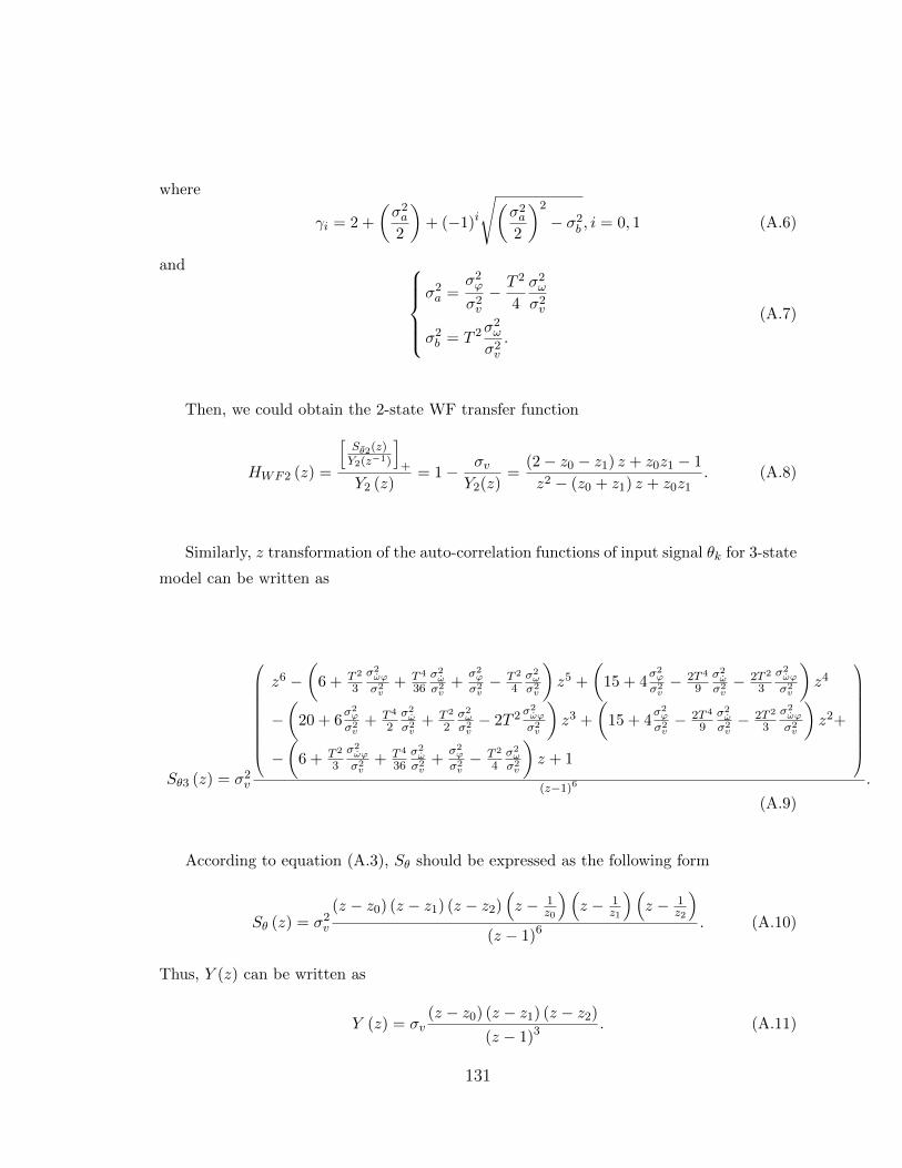
where
γi = 2 +
(σ2a
2
)+ (−1)i
√(σ2a
2
)2
− σ2b , i = 0, 1 (A.6)
and σ2a =
σ2ϕ
σ2v
− T 2
4
σ2ω
σ2v
σ2b = T 2σ
2ω
σ2v
.
(A.7)
Then, we could obtain the 2-state WF transfer function
HWF2 (z) =
[Sθ2(z)Y2(z−1)
]+
Y2 (z)= 1− σv
Y2(z)=
(2− z0 − z1) z + z0z1 − 1
z2 − (z0 + z1) z + z0z1. (A.8)
Similarly, z transformation of the auto-correlation functions of input signal θk for 3-state
model can be written as
Sθ3 (z) = σ2v
z6 −(
6 + T 2
3
σ2ωϕ
σ2v
+ T 4
36σ2ωσ2v
+σ2ϕ
σ2v− T 2
4σ2ωσ2v
)z5 +
(15 + 4
σ2ϕ
σ2v− 2T 4
9σ2ωσ2v− 2T 2
3
σ2ωϕ
σ2v
)z4
−(
20 + 6σ2ϕ
σ2v
+ T 4
2σ2ωσ2v
+ T 2
2σ2ωσ2v− 2T 2 σ
2ωϕ
σ2v
)z3 +
(15 + 4
σ2ϕ
σ2v− 2T 4
9σ2ωσ2v− 2T 2
3
σ2ωϕ
σ2v
)z2+
−(
6 + T 2
3
σ2ωϕ
σ2v
+ T 4
36σ2ωσ2v
+σ2ϕ
σ2v− T 2
4σ2ωσ2v
)z + 1
(z−1)6 .
(A.9)
According to equation (A.3), Sθ should be expressed as the following form
Sθ (z) = σ2v
(z − z0) (z − z1) (z − z2)(z − 1
z0
)(z − 1
z1
)(z − 1
z2
)(z − 1)6 . (A.10)
Thus, Y (z) can be written as
Y (z) = σv(z − z0) (z − z1) (z − z2)
(z − 1)3 . (A.11)
131

Expanding equation (A.10), we obtain
Sθ (z) = σ2v
(z2 −
(z0 + 1
z0
)z + 1
)·(z2 −
(z1 + 1
z1
)z + 1
)·(z2 −
(z2 + 1
z2
)z + 1
) (z − 1)6 . (A.12)
Denoting r0, r1 and r2 as
r0 =
(z0 +
1
z0
)r1 =
(z1 +
1
z1
)r2 =
(z2 +
1
z2
) (A.13)
and by solving the quadratic equation, the roots of Sθ can be obtained as
zi =ri ±√ri2 − 4
2, i ∈ {0, 1, 2} . (A.14)
Among these 6 roots, only three of them are located inside the unit circle and the rest are
located outside the unit circle. Their locations depend on ri and ri and can be solved by
the following steps.
First, we substitute ri into Sθ to obtain:
Sθ (z) = σ2v
(z2 − r0z + 1)(z2 − r1z + 1)(z2 − r2z + 1)
(z − 1)6
= σ2v
z6 − (r0 + r1 + r2) z5 + (r0r1 + r1r2 + r0r2 + 3) z4
− (r0r1r2 + 2 (r0 + r1 + r2)) z3
+ (r0r1 + r1r2 + r0r2 + 3) z2 − (r0 + r1 + r2) z + 1
(z − 1)6 .
(A.15)
Then, by comparing the above equation to equation (A.9), we have
r0 + r1 + r2= 6+T 2
3
σ2ωϕ
σ2v
+T 4
36
σ2ω
σ2v
+σ2ϕ
σ2v
− T 2
4
σ2ω
σ2v
r0r1 + r1r2 + r0r= 12 + 4σ2ϕ
σ2v
− 2T 4
9
σ2ω
σ2v
− 2T 2
3
σ2ωϕ
σ2v
r0r1r2= 8+4σ2ϕ
σ2v
+4T 4
9
σ2ω
σ2v
+ T 2σ2ω
σ2v
− 8T 2
3
σ2ωϕ
σ2v
.
(A.16)
132

The above three equations indicate that r0, r1 and r2 are the three roots of (z + r0) (z + r1) (z + r2) =
0. To solve this cubic equation the Cardano’s Formula is applied and ri can be expressed
in the following forms
r0 = 2 + x+3
√y +
√y2 +m3 +
3
√y −
√y2 +m3 (A.17)
r1 = 2 + x+−1 +
√3j
2
3
√y +
√y2 +m3 +
−1−√
3j
2
3
√y −
√y2 +m3 (A.18)
r2 = 2 + x+−1−
√3j
2
3
√y +
√y2 +m3 +
−1 +√
3j
2
3
√y −
√y2 +m3. (A.19)
Then we have r0 + r1 + r2 = 6 + 3x
r0r1 + r1r2 + r0r2 = 12 + 12x+ 3x2 + 3m
r0r1r2 = 8 + 12x+ 2y + 6x2 + x3 + 3xm+ 6m.
(A.20)
Comparing equation (A.20) to equation (A.16), x, y and m can be determined as belowx = d/3
y = 2d+1
27d3 − f +
2
3d2 − 1
6df +
1
2g
m = (3f − 12d− d2)/9
(A.21)
with
d =T 2
3
σ2ωϕ
σ2v
+T 4
36
σ2ω
σ2v
+σ2ϕ
σ2v
− T 2
4
σ2ω
σ2v
g = 4σ2ϕ
σ2v
+4T 4
9
σ2ω
σ2v
+ T 2σ2ω
σ2v
− 8T 2
3
σ2ωϕ
σ2v
f = 4σ2ϕ
σ2v
− 2T 4
9
σ2ω
σ2v
− 2T 2
3
σ2ωϕ
σ2v
.
(A.22)
Finally, z0, z1 and z2 are solved and can be written as
zi =ri ±
√r2i − 4
2, i = 0, 1, 2 (A.23)
Equation (A.23) has 6 roots due to the additional parameter qa’s effect on the roots’
locations. Among the 6 roots, only three of them are located inside the unit circle and the
rest are located outside circle. To keep the loop stable, z0, z1 and z2 should be the roots
133

inside or on the unit circle.
Then, we could obtain the 3-state WF transfer function
HWF3 (z) =
[Sθ3(z)Y3(z−1)
]+
Y3 (z)
= 1− σvY3(z)
=(3− z0 − z1 − z2) z2 + (z0z1 + z0z2 + z1z2 − 3) z + 1− z0z1z2
z3 + (−z0 − z1 − z2) z2 + (z0z1 + z0z2 + z1z2) z − z0z1z2.
(A.24)
134

Appendix B
Frequency Measurement
Derivation
According to equations (3.14) and (3.17) ,
∆θk+1 −∆θk =T
2∆ωk+1 + ∆ϕk+1 + vk+1 −
T
2∆ωk −∆ϕk − vk
=T
2∆ωk+1 + T∆ωk + ∆ϕk + vk+1 −
T
2∆ωk −∆ϕk − vk
=T
2(∆ωk+1 + ∆ωk) + vk+1 − vk
(B.1)
Assuming that the frequency error will not change by a significant amount over one sample
period, we have
∆θk+1 −∆θk ≈ T∆ωk+1 + vk+1 − vk (B.2)
Similarly, according to equations (3.15) and (3.17),
∆θk+1 −∆θk =T 2
6∆ωk+1 +
T
2∆ωk+1 + ∆ϕk+1 + vk+1 −
T 2
6∆ωk −
T
2∆ωk −∆ϕk − vk
=T 2
6∆ωk+1 +
T
2∆ωk+1 +
T 2
2∆ωk + T∆ωk + ∆ϕk + vk+1
− T 2
6∆ωk −
T
2∆ωk −∆ϕk − vk
=
(T 2
6∆ωk+1 +
T 2
2∆ωk −
T 2
6∆ωk
)+T
2(∆ωk+1 + ∆ωk) + vk+1 − vk
(B.3)
135

Again, assuming that the frequency error and frequency rate error will not change by a
significant amount over one sample period, we have
∆θk+1 −∆θk ≈T 2
2∆ωk+1 + T∆ωk+1 + vk+1 − vk (B.4)
136

Appendix C
Frequency Tracking Error
Covariance Matrix Derivation
Substituting the received and local generated signal in equations (4.1), (4.12) and (4.18)
into the equation (4.29), we have
Pk+1 = E[(xk+1 − xk+1) (xk+1 − xk+1)T
]= E
[(AFxk + nk −AF xk −AFL∆$k) (AFxk + nk −AF xk −AFL∆$k)
T]
= E
(AF∆xk + nk −AFL (HF∆xk + uk))
(AF∆xk + nk −AFL (HF∆xk + uk))T
= AF (I− LHF )E
[∆xk∆xk
T]
(I− LHF )TATF + 2AFL(AFL)T σ
2v
T 2
+ QF −AF (I− LHF )E[∆xkuk
T]
(AFL)T −AFLE[uk∆xk
T]
(I− LHF )TATF
(C.1)
Let Gk represents the correlation between the error state and non-white measurement
noise, we have Gk = E[∆xkuk
T]
and GTk = E
[uk∆xk
T]. When k approaches infinity,
137

Gk+1 = Gk = GY is in steady state. We expand GY as following steps
GY = E[∆xkuk
T]
= E
[−(AF xk−1 + AFL∆$k−1)
(vk − vk−1)T
T
]
= E
[−AFL
(vk−1 − vk−2)
T
(vk − vk−1)T
T
]
= AFLσ2v
T 2
(C.2)
Finally, we can obtain
PY = AF (I− LHF )PY (I− LHF )TATF + QF + 2AFL(AFL)T σ
2v
T 2
+ AF (I− LHF )GY (AFL)T + AFLGTY (I− LHF )TAT
F
= AF (I− LHF )PY (I− LHF )TATF + QF + 2AFL(AFL)T σ
2v
T 2
−AF (I− LHF )AL(AFL)T σ2v
T 2−AFL(AFL)T(I− LHF )TAT
F
σ2v
T 2
(C.3)
138

Appendix D
Optimal solution of 1-state
frequency tracking loop
To solve the quartic equation α4 − 4α3 − bα+ b = 0, we denote α = x+ 1 to eliminate the
term α3 in this quartic equation and then we have
x4 + 6x2 − (b+ 8)x− 3 = 0. (D.1)
Applying the Ferrari’s solution, the four solutions of the above equation can be obtained as
x1 =1
2
√4 +
3√b2 + 16b− 1
2
√8− 3
√b2 + 16b+
2b+ 16√4 + 3√b2 + 16b
(D.2)
x2 =1
2
√4 +
3√b2 + 16b+
1
2
√8− 3
√b2 + 16b+
2b+ 16√4 + 3√b2 + 16b
(D.3)
x3 = −1
2
√4 +
3√b2 + 16b− 1
2
√8− 3
√b2 + 16b− 2b+ 16√
4 + 3√b2 + 16b
(D.4)
x4 = −1
2
√4 +
3√b2 + 16b+
1
2
√8− 3
√b2 + 16b− 2b+ 16√
4 + 3√b2 + 16b
(D.5)
The corresponding solutions of α can be obtained through the relation α = x + 1. It is
noted that the tracking error variance pω should be always positive. The condition that
139

0 < α < 2 should be satisfied. Hence, the optimal value of α that minimizes pω is
αopt = 1 +1
2
√4 +
3√b2 + 16b− 1
2
√8− 3
√b2 + 16b+
2b+ 16√4 + 3√b2 + 16b
. (D.6)
140