26 InsideGNSS j a n u a r y / f e b r u a r y 2 0 1 2 www.insidegnss

GNSS Solutions:

How can pseudorange measurements be generated from code tracking?

E very GNSS receiver processes the received signals to obtain an estimate of the propaga-tion time of the signal from

the satellites to the receiver. These propagation times are then expressed in meters to solve for the user position using trilateration.

Because the resulting distances are not only related to the distance between the receiver antenna and the satellites, i.e. the range, but also to an imperfect alignment of the receiver’s time scale to the GPS time scale, they are called pseudoranges.

Once a GNSS receiver’s acquisition stage has aligned the received and the locally generated code within less than a half chip period, a fine, closed-loop synchronization takes over and keeps the two codes aligned. Generally, the tracking system in GNSS receivers consists of a delay lock loop (DLL) for code tracking and a phase lock loop (PLL) for carrier phase tracking.

The measurements produced by the DLL are the pseudoranges. The PLL generates carrier phase measurements, which can be used on their own or to smooth the “raw” pseudorange measurements from the DLL. In the context of this article, we will only consider code-based pseudoranges.

Considering Galileo E1 or GPS L1, the code itself is characterized by the so-called integer ambiguity problem. This means that, without additional information, a single period of a code

(one-millisecond duration for L1, four milliseconds for E1) cannot be distinguished from any other code period, and as such, when computing travel-time differences among the tracked signals, these differences can only be obtained modulo the length of the code.

Fortunately, in the case of code measurements we can easily solve this integer ambiguity by exploiting the navigation message structure. Once the receiver is effectively tracking a signal, it also decodes the navigation message and achieves frame synchronization.

A counter is then associated to every single channel, so that each sample is labeled with a chip (code phase), a bit (within a navigation message subframe), and a subframe number. The receiver can then use these counters and the code phase measured in the DLL to compute the propagation times.

In the following discussion, we will consider the two main techniques that can be adopted to compute travel times on the basis of counter values.

Common Reception TimeThe common reception time method is usually implemented in commercial receivers. It estimates the pseudoranges by setting a common reception time across all the channels. This is equiva-lent to taking a snapshot of all the channels’ counters at a given time.

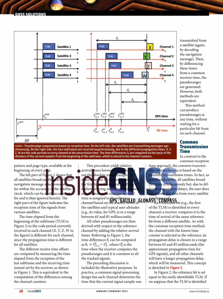
figure 1 illustrates this technique. Before describing the figure in detail, please note that in the following discussion we will often refer to the telemetry (TLM) word, which is always the first word of every GPS subframe and is characterized by its first eight bits (i.e., the preamble). With this TLM word, a receiver can easily identify the beginning of the subframe and use the TLM to define the counters as the distance of the current sample from the beginning of the current subframe. In the case of Galileo, a structure similar to the GPS subframe can be found in the F/NAV synchronization

Code Tracking &

Pseudoranges“GNSS Solutions” is a

regular column featuring questions and answers

about technical aspects of GNSS. Readers are invited to send their questions to

the columnist, Dr. Mark Petovello, Department of

Geomatics Engineering, University of Calgary, who will find experts to answer

them. His e-mail address can be found with

his biography at the conclusion of the column.

28 InsideGNSS j a n u a r y / f e b r u a r y 2 0 1 2 www.insidegnss

pattern and page type, available at the beginning of every page.

The left part of Figure 1 shows that all satellites broadcast the start of their navigation message synchronously (to within the accuracy of the satellite clock, which can be easily accounted for and is thus ignored herein). The right part of the figure indicates the reception time of the signals from various satellites.

The time elapsed from the beginning of the subframe (TLM in Figure 1) to the code period currently received in each channel (X, Y, Z, W in the figure) is different for each channel, since the propagation time is different for all satellites.

The different receive time offsets are computed by measuring the time elapsed from the reception of the last subframe and the receiving time instant set by the receiver, as shown in Figure 1. This is equivalent to the computation of the differences among the channel counters.

This procedure yields relative arrival times between satellites, but not the absolute pseudoranges. To determine the set of pseudoranges for the first time, the channel with the earliest arriving subframe is assumed as reference and a minimum travel time is assigned to the reference channel based on the known orbits of the satellites and typical user altitudes (e.g., its value, for GPS, is in a range between 65 and 85 milliseconds).

All other pseudoranges are then derived with respect to the reference channel by adding the relative-arrival times. Referring to Figure 1, the time differences δi can be computed as , where is the time when the receiver computes the pseudoranges and it is common to all the tracked signals.

The preceding discussion is included for illustrative purposes. In practice, a common signal-processing design has each channel determine the time that the current signal sample was

transmitted from a satellite (again, by decoding the navigation message). Then, by differencing these times from a common receiver time, the pseudoranges are generated. However, both methods are equivalent.

This method can produce pseudoranges at any time, without waiting for a particular bit front on each channel.

Common Transmission TimeIn contrast to the common reception

time approach, the common transmis-sion time technique is based on the satellites’ transmission times. In fact, as mentioned earlier, all satellites broad-cast data synchronously but, due to dif-ferent propagation delays, the user does not receive the data from every satellite synchronously.

As a reference bit (e.g., the first of the TLM) is identified in every channel, a receiver compares it to the time of arrival of the same reference bit from a different satellite. As with the common reception time method, the channel with the lowest time counter is selected as the reference, its propagation delay is chosen in a range between 65 and 85 milliseconds (the approximate propagation time for GPS signals), and all other channels will have a longer propagation delay, which will be measured. This concept is sketched in figure 2.

In Figure 2, the reference bit is set equal to the easily identifiable TLM. If we suppose that the TLM is identified

FIGURE 1 Pseudorange computation based on reception time. On the left side, the satellites are transmitting messages syn-chronously. On the right side, the four subframes are received asynchronously, due to the different propagation times. X, Y, Z, W are the code periods in every channel at the observation time. The time differences δi are computed on the basis of the distance of the current samples from the beginning of the subframe, which is stored in the channel counters.

GNSS SOLUTIONS

A T R I M B L E C O M P A N Y

A T R I M B L E C O M P A N Y

ashtech_Ad_InsideGNSS_8x10.75.indd 1 1/18/12 10:43 AM

32 InsideGNSS j a n u a r y / f e b r u a r y 2 0 1 2 www.insidegnss

for all the tracked satellites, then the receiver measures the time difference between the arrival times of the TLM for each satellite relative to the reference satellite. Referring to Figure 2, this time difference δi can therefore be written as , where

represents the time of reception of the subframe for the i-th satellite, while

is the time relative to the reference satellite.

With these time differences, the pseudoranges can be written as

, where Δb is the time scale bias between the receiver clock and the ones on board of the satellites, c is the speed of light, ρ1 is the pseudorange relative to the reference channel and δi is the delay of the i-th satellite channel with respect to the reference satellite.

This kind of approach has some disadvantages when implemented in a real-time receiver:a) It requires waiting until all the channels have received the

same data bit to compute the pseudoranges. b) Since the reference bit from each satellite arrives at a

different time instant, in general, the receiver will have different clock errors at each epoch resulting from the integration of the receiver oscillator’s frequency offset. That said, if the receiver’s oscillator is sufficiently stable, this will not introduce significant errors.

c) In case of a joint GPS/Galileo scenario, this technique is unfeasible in real-time implementations, because the receiver would have to work with two independent satellite systems, characterized by different data structures, and two separate reference channels (one for GPS and one for Galileo). Consequently, this approach would force the receiver to keep a large amount of information in a buffer, with a significant waste of resources as well as a non-negligible delay in the position, velocity, and time (PVT) computation.

Comparative ResultsWithout considering their respective pros and cons, the two different approaches are virtually equivalent in terms of computed pseudoranges as long as the receiver clock drift is relatively small. In figure 3 we show the difference between

the pseudoranges obtained using the two techniques, taking as an example the PRN30 GPS satellite.

Because the pseudoranges are not computed at the same time, we needed to interpolate the results obtained with the common reception time method. As can be seen, the differences are relatively small and within the expected level

GNSS SOLUTIONS

FIGURE 3 Comparison between pseudoranges computed by using common reception time and common transmission time

25

20

15

10

5

0

-5

-10

-15

-20

-25

Di�

eren

ce (m

)

3.1174 3.1175 3.1176 3.1177

Time (s) x 105

FIGURE 2 Pseudorange computation based on transmission. On the left side, the satellites are transmitting mes-sages synchronously. On the right side, the four subframes are received asynchronously, due to the different propagation time. The TLM word is taken as a referene. The time differences δi are computed on the basis of the relative arrival times of the front of the first bit of the TLM word.

www.insidegnss.com j a n u a r y / f e b r u a r y 2 0 1 2 InsideGNSS 33

of noise for this particular receiver. The pseudoranges obtained

using the two different methods are sometimes slightly different, but the receiver positions obtained using one or the other of the two methods are similar, and the variance in the accuracy of the position along the three axes X, Y, Z has the same magnitude in both cases, as can be seen in figure 4.

SummaryAs expected, the both methods of gener-ating pseudorange measurements yield statistically identical measurements and computed position estimates. However, from a receiver designer point of view, the common reception time method

is more suitable for implementation, because the pseudorange measurements

are performed at the same time instant for all the channels, while the common transmission time technique can be considered more didactic and intuitive.

AuthorsMaRCo Rao, PH.D., is a grantholder at the European Commission (EC) Joint Research Centre (JRC). His research interests are in GNSS receiver design,

Kalman filtering, and tracking.

GIaNlUCa FalCo, PH.D., is a researcher at the NavSAS Laboratory – Istituto Superiore Mario Boella in Turin, Italy. His research interests are in GNSS software receivers

and scatterometry. FIGURE 4 Comparison between the estimated positions along the three ECEF axes.

4.19864.19844.1982EC

EF-X

(m)

Time-TOW (s)

x 105

x 106

3.1175 3.1185 3.1195 3.1205

9.5749.672

9.679.668EC

EF-Y

(m)

x 105

x 105

3.1175 3.1185 3.1195 3.1205

4.68834.68824.6881

4.6884.6679EC

EF-Z

(m)

x 105

x 106

3.1175 3.1185 3.1195 3.1205

LS Position computation through di�erent methods for pseudoranges estimation

Mark Petovello is an Associate Professor in the Department of Geomatics Engineering at the University of Calgary. He has been actively involved in many aspects of positioning and navigation since 1997 including GNSS algorithm development, inertial navigation, sensor integration, and software development.

Email: mark.petovello@ucalgary.ca

ANTENNA SOLUTIONS FOR DEFENSE AND NETWORK TIMING APPLICATIONS

Aviation Asset Tracking and Communications

Munitions Guidance

PCTEL designs and manufactures high performance antennas to provide precise operation, maximum durability, and ease of installation.

■ High Out-of-Band Rejection Solutions For Extreme RF Interference Environments

■ GPS L1, L2, L5 GLONASS, GALILEO, Beidou, Iridium, Globalstar and Inmarsat Designs

■ Critical Applications Including Munitions Guidance, Aviation, Precision Agriculture, Network Timing & Asset/Radio Mount Tracking

A LEADING PROVIDER OF HIGH PERFORMANCE ANTENNAS FOR DEFENSEOF HIGH PERFORMANCE ANTENNAS FOR DEFENSE

phone 630.372.6800 toll-free 800.323.9122 website www.antenna.comemail antenna.sales@pctel.com

119743 PCTEL_GNSS_Q112_3sq.indd 1 1/10/12 10:45 AM