a new three-axis vibrating sample magnetometer for

www.elsevier.com/locate/epsl

Earth and Planetary Science L

A new three-axis vibrating sample magnetometer for continuous

high-temperature magnetization measurements: applications

to paleo- and archeo-intensity determinations

Maxime Le Goff*, Yves Gallet

Departement de Geomagnetisme et Paleomagnetisme, UMR CNRS 7577, Institut de Physique du Globe de Paris,

4 Place Jussieu, 75252 Paris cedex 05, France

Received 13 May 2004; received in revised form 18 October 2004; accepted 18 October 2004

Available online 21 November 2004

Editor: R.D. van der Hilst

Abstract

We have developed a new three-axis vibrating sample magnetometer, which allows continuous high-temperature

magnetization measurements of individual cylindrical ~0.75 cm3 samples up to ~650 8C and the acquisition of thermoremanent

magnetization (TRM) in any direction and field intensity up to 200 AT. We propose a fast (less than 2.5 h) automated

experimental procedure adapted from Boyd’s [Nature 319 (1986) 208–209] modified version of the Thellier and Thellier [Ann.

Geophys. 15 (1959) 285–376] method which provides continuous intensity determinations over a large (typically 300 8C)temperature interval for each sample. This procedure allows one to take into account both the cooling rate dependence of TRM

acquisition and anisotropy of TRM. Several examples of analyses of ancient magnetization demonstrate the quality and

reliability of the data and illustrate the promising potential of this new instrument in paleo- and archeomagnetism.

D 2004 Elsevier B.V. All rights reserved.

Keywords: magnetometer; paleo-intensity; archeomagnetism; cooling rate; anisotropy

1. Introduction

Deciphering the dynamical processes generating

the Earth’s magnetic field requires a complete

description both in direction and intensity of the

temporal geomagnetic variations at various time

0012-821X/$ - see front matter D 2004 Elsevier B.V. All rights reserved.

doi:10.1016/j.epsl.2004.10.025

* Corresponding author. Tel.: +33 1 4511 4184; fax: +33 1

4511 4190.

E-mail address: [email protected] (M. Le Goff).

scales. Our knowledge of geodynamo evolution is

presently strongly biased in favour of the directional

variations as paleo- and archeo-intensity data are still

scarce and not always of sufficient quality. For

instance, it remains difficult to ascertain very long

term intensity changes [3] and to untangle with some

confidence any evolution linked to changes in geo-

magnetic reversal frequency (e.g., see [4]). The

sawtooth pattern apparently seen in relative paleo-

intensity from sediments [5] has also not yet been

etters 229 (2004) 31–43

M. Le Goff, Y. Gallet / Earth and Planetary Science Letters 229 (2004) 31–4332

satisfactorily tested from absolute intensity determi-

nations. These uncertainties clearly leave open the

possibility that some important properties of the

geomagnetic field could actually be unknown.

The scarcity of the absolute intensity data obtained

either from volcanic rocks or baked archeological

materials mainly results from the fact that most

available investigation procedures are laborious and

often unproductive due to poor data quality. The

principal method, relying on the additive property of

partial TRM (pTRM), was proposed by Thellier and

Thellier [2]. It consists of progressively replacing the

original TRM (i.e., the natural remanent magnet-

ization NRM) by a new one acquired under known

laboratory field conditions. Although rather old, this

method and its principal variant [6] are generally

considered the most reliable paleo-intensity techni-

ques, as long as tests for judging magnetic mineralogy

stability with the heating of the samples are con-

ducted. In these experiments, the samples are repeat-

edly heated to increasing temperatures, with typically

~20 to 30 heating–cooling cycles lasting at least 1 h

each. Such a time-consuming procedure requires a

large amount of magnetization measurements but

often has a poor success rate because of mineral

alteration during heating. To diminish the time of

heating and hopefully the possibility for alteration,

Shaw [7] proposed a mixed thermal and alternating

field (AF) method involving only one heating–cooling

cycle at high temperature (~600 8C). In this method,

the NRM is demagnetized using alternating fields

replaced in one thermal step by a new laboratory bfullQTRM which is then also AF demagnetized. This

procedure is faster than the previous one, but it is not

clear whether the success rate is increased (e.g., see

[8]). In most cases, one heating at high temperature is

sufficient to significantly alter the magnetic mineral-

ogy of the samples. To better circumvent the problem

of alteration, Walton et al. [9,10] proposed a radically

different method based on microwave demagnetiza-

tion. They indeed showed that microwaves emitted at

frequencies z8 GHz (up to 14 GHz presently) are

efficient to quickly and completely demagnetize (and

remagnetize) samples without significantly heating

the samples (b~150 8C). Several recent studies

presented satisfactory comparisons between intensity

results obtained rapidly using the microwave techni-

que and much slower using the Thellier and Thellier

method (e.g., see [11]). This makes the microwave

technique, which is still under technological and

methodological development, very promising but

rather expensive.

However, we would like to point out the poor

understanding of the theory behind microwave tech-

nique; a theoretical relationship with Neel’s [12]

theory of thermal activitation of magnetic moments

is not established yet, and thus, the analogy between

microwave and thermal remanence magnetization

remains based on experimental measurements. For

this reason, we have developed another relatively fast

procedure, which retains the principal characteristics

of the Thellier and Thellier method. We have

constructed a new three-axis vibrating sample mag-

netometer (that we call Triaxe) comprising a small

oven placed in the center of a group of 10 pickup

coils, all of these being inserted inside three perpen-

dicular Helmholtz coils. This equipment allows

continuous high-temperature (up to ~650 8C) magnet-

ization measurements of individual cylindrical ~0.75

cm3 samples and the acquisition of TRM in any

direction and field intensity up to 200 AT. In this first

paper, we present a brief description of the instrument,

the methodology used to obtain paleo- and arche-

ointensity data and several examples of reliable results

obtained in less than 2.5 h.

2. Description of the new instrument

The magnetometer comprises three orthogonal sets

of pickup coils necessary for measuring the magnet-

ization of a sample, which vibrates horizontally along

a single direction (Fig. 1). Two coaxial coils in

opposition are sufficient for detecting the magnetic

component along the vibration axis, while two

coplanar pairs of coils in opposition are necessary

for each perpendicular magnetic component. Both the

distance between the coils or the pairs of coils and the

size of these coils were carefully designed to insure

the most homogeneous and linear electromagnetic

effect through the entire displacement volume of the

sample. This sensor system is devised for measuring

the magnetization of a cylindrical 1-cm-long/1-cm-

diameter sample vibrating with a frequency of 11.18

Hz and with a net displacement amplitude of 1 cm. Its

sensitivity is better than 10�8 Am2 (~10�2 A/m) in all

Fig. 1. Schematic of the new three-axis vibrating sample magnetometer. The instrument includes a small oven and its radiator inserted within

three orthogonal sets of pickup coils; the whole assemblage is placed inside three Helmholtz coils and a three-layer Ametal shield. This

instrument allows continuous high temperature measurements of remanent or induced magnetization for a cylindrical (0.75 cm3) sample.

M. Le Goff, Y. Gallet / Earth and Planetary Science Letters 229 (2004) 31–43 33

three directions, thus allowing magnetization meas-

urements of most volcanic rocks and baked archeo-

logical materials. A small oven and its water-cooling

system are placed in the center of the pickup coil

assembly, that is made easier by the square shape of

the 10 coils (Fig. 1). The heating, up to ~650 8C, isproduced by a 2.5-kHz alternating current in a bifilar

resistor avoiding electromagnetic interference in the

pickup coils. The heating and the cooling rates can be

adjusted up to a maximum of 60 8C/min. The sensor

and heating–cooling systems are centered inside three

perpendicular Helmholtz coils coaxial with the mag-

netometer axes. This permits the generation of a

magnetic field up to 200 AT in any direction, in

particular, towards the NRM direction of the studied

samples. Finally, the complete system except the

linear step-by-step motor producing the horizontal

sinusoidal displacement of the sample is inserted in a

three-layer Ametal cylindrical shield.

We point out that one of the technical difficulties

was to ensure the isotropy of both magnetization

measurements and field intensity generation together

with the best possible alignment between the sensor

and Helmholtz coil axes. To test this, we carried out

magnetic measurements on a pure paramagnetic

sample made of 1 g of Holmium oxide in a field

of 150 AT (yielding a magnetization of about

~40.10�8 Am2). These measurements have shown

an angular alignment better than 1.58 in all three

directions.

3. Methodology used for paleo- and

archeo-intensity measurements

There are only a few studies presenting examples

of natural TRM measurements at high temperatures in

the literature (e.g., see [1,13–17]). We can, however,

find a detailed description of intensity determinations

from such measurements in Boyd [1] and Tanaka et al.

[17]. In the present paper, we will use the high-

temperature version of the Thellier and Thellier [2]


method modified by Coe [6], as described in Boyd [1]

and Tanaka et al. [17]. Its main difference with the

classical method, which involves stepwise magnet-

ization measurements at room temperature, is that it

requires, for each studied sample, an investigation of

the temperature dependence of the spontaneous

magnetization (Js). This is necessary to separate the

fraction of magnetization unblocked (or blocked)

between two temperatures from the thermal decay of

the magnetization fraction remaining blocked.

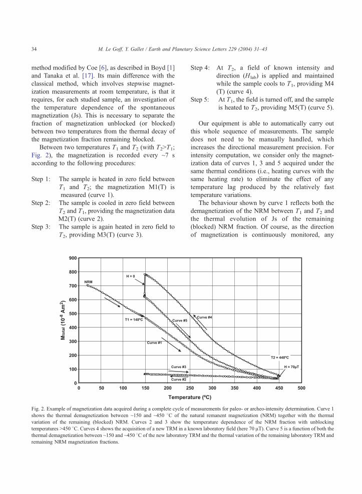
Between two temperatures T1 and T2 (with T2NT1;

Fig. 2), the magnetization is recorded every ~7 s

according to the following procedures:

Step 1: The sample is heated in zero field between

T1 and T2; the magnetization M1(T) is

measured (curve 1).

Step 2: The sample is cooled in zero field between

T2 and T1, providing the magnetization data

M2(T) (curve 2).

Step 3: The sample is again heated in zero field to

T2, providing M3(T) (curve 3).

Fig. 2. Example of magnetization data acquired during a complete cycle of

shows the thermal demagnetization between ~150 and ~450 8C of the

variation of the remaining (blocked) NRM. Curves 2 and 3 show the

temperatures N450 8C. Curves 4 shows the acquisition of a new TRM in a k

thermal demagnetization between ~150 and ~450 8C of the new laboratory

remaining NRM magnetization fractions.

Step 4: At T2, a field of known intensity and

direction (Hlab) is applied and maintained

while the sample cools to T1, providing M4

(T) (curve 4).

Step 5: At T1, the field is turned off, and the sample

is heated to T2, providing M5(T) (curve 5).

Our equipment is able to automatically carry out

this whole sequence of measurements. The sample

does not need to be manually handled, which

increases the directional measurement precision. For

intensity computation, we consider only the magnet-

ization data of curves 1, 3 and 5 acquired under the

same thermal conditions (i.e., heating curves with the

same heating rate) to eliminate the effect of any

temperature lag produced by the relatively fast

temperature variations.

The behaviour shown by curve 1 reflects both the

demagnetization of the NRM between T1 and T2 and

the thermal evolution of Js of the remaining

(blocked) NRM fraction. Of course, as the direction

of magnetization is continuously monitored, any

measurements for paleo- or archeo-intensity determination. Curve 1

natural remanent magnetization (NRM) together with the thermal

temperature dependence of the NRM fraction with unblocking

nown laboratory field (here 70 AT). Curve 5 is a function of both theTRM and the thermal variation of the remaining laboratory TRM and


sample which would show directional variations at

this step would be rejected. Curve 5 also shows a

combination between the demagnetization (again

between T1 and T2) of the new TRM imparted

during step 4 under a known laboratory field (Hlab)

and the thermal evolution of Js of the remaining

blocked magnetic fraction (laboratory TRM+NRM).

Curve 3 represents the temperature dependence

between T1 and T2 of the NRM fraction with

unblocking temperatures NT2.

Hence, at any discrete temperature Ti between T1

and T2, the NRM and laboratory TRM fractions

(D1(Ti), D5(Ti), respectively) whose unblocking tem-

peratures are between Ti and T2, are obtained from

D1 Tið Þ ¼ M1 Tið Þ �M3 Tið Þ ð1Þ

D5 Tið Þ ¼ M5 Tið Þ �M3 Tið Þ ð2Þ

and the ancient field intensity can be derived from the

formula

R Tið Þ ¼ Hlab4D1 Tið Þ=D5 Tið Þ ð3Þ

Another possibility neither explored by Boyd [1]

nor Tanaka et al. [17] is to estimate the NRM and

laboratory TRM fractions unblocked between T1 and

Ti. In contrast with the previous computations for

which we compare two pTRM at the same temper-

ature Ti (see Eqs. (1) and (2)), we now consider the

decrease in magnetization between two temperatures

T1 and Ti, thus including both the demagnetization of

the pTRM and the thermal dependence of Js. These

computations require us to make an approximation

because the variation in Js between T1 and Ti of the

magnetic fraction with unblocking temperatures

between Ti and T2 is not known. There are two

possibilities. The first is to consider that the behaviour

of the curve 3 between T1 and Ti provides a proxy for

the Js variation. We then can write:

D1V Tið Þ ¼ M1 T1Þ � M3 T1Þ=M3 Tið Þð Þ4M1 Tið Þððð4Þ

D5V Tið Þ ¼ M5 T1Þ � M3 T1Þ=M3 Tið Þð Þ4M5 Tið Þððð5Þ

As the remaining fraction above T2 is small, the

second possibility is to simply neglect the variation in

Js because M3(T) does not provide the necessary

constraints. In this case:

D1V Tið Þ¼ M1 T1Þ�M1 Tið Þð Þ� M3 T1Þ �M3 Tið Þð Þððð6Þ

D5V Tið Þ¼ M5 T1Þ�M5 Tið Þð Þ � M3 T1Þ �M3 Tið Þð Þððð7Þ

In both cases, the ancient field intensity can be

obtained from:

RV Tið Þ ¼ Hlab4DV1 Tið Þ=D5V Tið Þ ð8Þ

It is worth noting that experiments carried out on

several archeological samples show that the differ-

ences in RV(Ti) induced by the two possibilities of

computations are very small (and especially negligible

when the variation of M3(T) is linear). In the present

study, we prefer to not consider any proxy for the Js

variation between T1 and Ti, and we use Eqs. (6) and

(7) to compute the ratio RV(Ti).Practically, both computations of R(Ti) and RV(Ti)

require the interpolation of the three data sets M1(T),

M3(T) and M5(T) to obtain data at the same temper-

ature Ti. A temperature interval of 5 8C is chosen,

which is very close to the mean interval of actual

measurements.

4. Testing the experimental procedure on

laboratory TRM

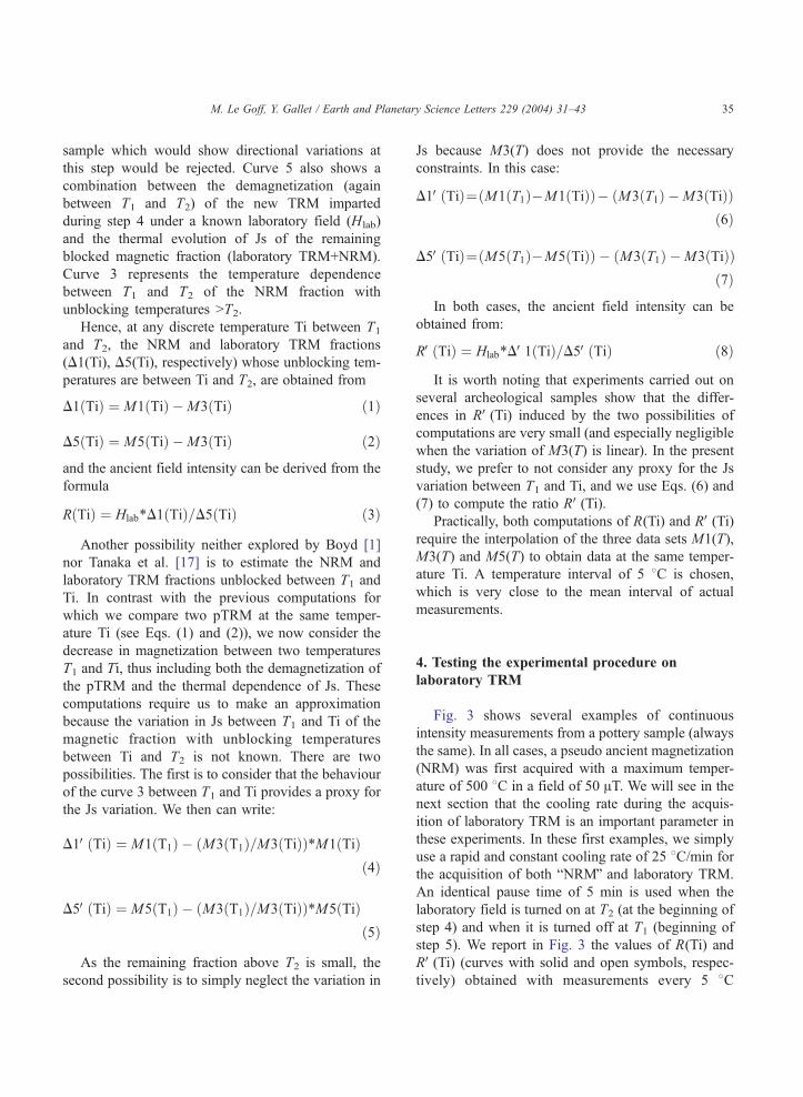
Fig. 3 shows several examples of continuous

intensity measurements from a pottery sample (always

the same). In all cases, a pseudo ancient magnetization

(NRM) was first acquired with a maximum temper-

ature of 500 8C in a field of 50 AT. We will see in the

next section that the cooling rate during the acquis-

ition of laboratory TRM is an important parameter in

these experiments. In these first examples, we simply

use a rapid and constant cooling rate of 25 8C/min for

the acquisition of both bNRMQ and laboratory TRM.

An identical pause time of 5 min is used when the

laboratory field is turned on at T2 (at the beginning of

step 4) and when it is turned off at T1 (beginning of

step 5). We report in Fig. 3 the values of R(Ti) and

RV(Ti) (curves with solid and open symbols, respec-

tively) obtained with measurements every 5 8C

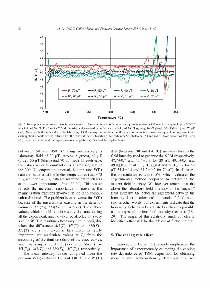
Fig. 3. Examples of continuous intensity measurements from a pottery sample in which a pseudo ancient NRM was first acquired up to 500 8Cin a field of 50 AT. The bancientQ field intensity is determined using laboratory fields of 20 AT (green), 40 AT (blue), 50 AT (black) and 70 AT(red). Note that both the NRM and the laboratory TRM are acquired in the same thermal conditions (i.e., same heating and cooling rates). For

each applied laboratory field, estimates of the bancientQ field intensity are derived every 5 8C between 150 and 450 8C from two ratios R(Ti) and

RV(Ti) (curves with solid and open symbols, respectively). See text for explanations.


between 150 and 450 8C using successively a

laboratory field of 20 AT (curves in green), 40 AT(blue), 50 AT (black) and 70 AT (red). In each case,

the values are quite constant over a large segment of

the 300 8C temperature interval, but the raw R(Ti)

data are scattered at the higher temperatures (last ~70

8C), while the RV(Ti) data are scattered but much less

at the lower temperatures (first ~30 8C). This scatter

reflects the increased importance of noise as the

magnetization fractions involved in the ratio compu-

tation diminish. The problem is even worse for R(Ti)

because of the uncertainties existing in the determi-

nation of M1(T2), M3(T2) and M5(T2). These three

values, which should remain exactly the same during

all the experiment, may however be affected by a very

small drift. The resulting effect may not be negligible

when the differences M1(T)�M3(T) and M5(T)�M3(T) are small. Even if this effect is rarely

important, we recalculate values at T2 from the

smoothing of the final one-third of the three curves,

and we simply shift D1(Ti) and D5(T i) by

M1(T2)�M3(T2) and M5(T2)�M3(T2), respectively.

The mean intensity values computed from the

previous R(Ti) (between 150 and 380 8C) and RV(Ti)

data (between 180 and 450 8C) are very close to the

field intensity used to generate the NRM (respectively,

48.7F0.7 and 49.4F0.5 for 20 AT, 49.1F0.4 and

49.4F0.3 for 40 AT, 50.3F0.4 and 50.1F0.2 for 50

AT, 51.4F0.4 and 51.7F0.2 for 70 AT). In all cases,

the concordance is within 5%, which validates the

experimental method proposed to determine the

ancient field intensity. We however remark that the

closer the laboratory field intensity to the bancientQfield intensity, the better the agreement between the

intensity determination and the bancientQ field inten-

sity. In other words, our experiments indicate that the

laboratory field must be adjusted as close as possible

to the expected ancient field intensity (see also [18–

20]). The origin of this relatively small but clearly

identified effect will be the subject of further studies.

5. The cooling rate effect

Genevey and Gallet [21] recently emphasized the

importance of experimentally estimating the cooling

rate dependence of TRM acquisition for obtaining

more reliable archeo-intensity determinations (see


also [22]). This effect is due to the fact that the baked

clay samples are cooled much more rapidly during

laboratory experiments than during their original

firing (the latter cooling could have lasted several

days), which generally leads to an overestimation of

the ancient field intensity [23–25].

In our experiments using baked clay samples, the

cooling rate effect can be illustrated by comparing the

values of the ratio R(Ti) (curves with solid symbols in

Fig. 4) obtained using successively a rapid (25 8C/min, black curve), a moderate (6 8C/min, blue curve)

and a slow (2 8C/min, green curve) cooling rate during

the laboratory TRM acquisition (step 4) in all cases

from the same initial conditions (a TRM acquired in

the same sample up to 500 8C in a field of 50 AT and

after a cooling time of 16 h). The three R(Ti) data sets

are determined between 150 and 450 8C. When the

sample is rapidly cooled, the values significantly and

smoothly increase with increasing temperatures start-

ing at 150 8C from a slightly overestimated field

intensity value in comparison with the expected

intensity and reaching strongly biased values at high

temperatures. This increasing trend is progressively

lowered when slower cooling rates are considered, but

Fig. 4. Effect of the cooling rate dependence of TRM acquisition in our exp

given by R(Ti) and RV(Ti) (curves with solid and open symbols, respectivel

min; in black), a moderate (6 8C/min; in blue) and a slow (2 8C/min; in gre

AT). In these three cases, the same initial NRM imparted in the same samp

long cooling time of 16 h). A fourth case (curves in red) shows the behavio

(6 and 60 8C/min, respectively). See text for further description and expla

it still exists for the cooling rate of 2 8C/min (to be

compared with the cooling rate of 0.5 8C/min for the

acquisition of the pseudo ancient NRM). We also

observe that the initial intensity value obtained at 150

8C becomes closer to the expected field intensity as

the cooling rate is decreased. The cooling rate effect

can also be illustrated by showing the R(T) data when

the cooling rate used for TRM acquisition is slower

than the one applied for NRM acquisition (6 and 60

8C/min, respectively). In clear contrast with the

previous cases, the values now show a significant

decreasing trend (red curve).

An option would be naturally to consider a very

slow cooling rate for the laboratory TRM acquisition,

but this would imply an unreasonably long duration

for intensity determinations. It is worth pointing out

that the trends in R(Ti) reflect the fact that the bias

produced by the small quantity of TRM not gained

between T2 and T1 because of a too rapid cooling rate

becomes stronger as the magnetization fractions with

unblocking temperatures between Ti and T2 progres-

sively diminish with increasing temperatures Ti. This

difficulty can be bypassed by considering the ratio

RV(Ti) which involves the magnetization fractions

eriments. We show the estimates of the pseudo ancient field intensity

y) obtained every 5 8C between 150 and 450 8C using a rapid (25 8C/en) cooling rate for the laboratory TRM acquisition (in a field of 50

le is analyzed (acquired up to 500 8C in a field of 50 AT and after a

ur when the laboratory TRM is acquired much slowly than the NRM

nation.


unblocked between T1 and Ti (thus increasing with

temperature). The values obtained for this ratio are

indeed in much better agreement with the expected

field intensity (Fig. 4). For each used cooling rate, the

most biased intensity value is observed at T2 (being

necessarily equal to the one obtained for R(Ti) at

Ti=T1). However, whatever the cooling rate, the

recovered intensity values are almost identical to the

expected intensity over a large part of the temperature

interval. Our experiments thus indicate that RV(Ti)provides a reliable estimate of the ancient field

intensity fairly independent of the cooling rate effect,

even when a cooling rate as fast as 25 8C/min is used

for laboratory TRM acquisition. The use of a slower

cooling rate appears unnecessary. This makes possible

a complete field intensity determination in less than

2.5 h for one sample.

6. Anisotropy of TRM

The anisotropy of TRM is known to be

important in most baked archeological materials

(e.g., see [21,22,26–28]). It has been demonstrated

by the fact that the direction of the TRM acquired

by a baked clay artifact, such as a brick or a

pottery, is often different from the direction of the

applied field. This deflection is generally consistent

with the existence of an easy plane of magnet-

ization induced by the manufacturing process (i.e.,

identical to the stretching plane). In the usual

procedure with magnetization measurements at

room temperature, the TRM anisotropy effect is

estimated for each sample by measuring partial

TRM acquired successively in six directions, which

allows the determination of the TRM anisotropy

tensor. A TRM anisotropy factor is then computed

[29] and used to correct the raw intensity value.

Another method consists in producing a TRM

closely in the direction (within 108) of the original

magnetization (NRM), which avoids the need to

quantify and correct the magnetization data for

TRM anisotropy (e.g., see [26,27]). In most cases,

except when the TRM anisotropy is too strong, this

is possible by simply applying the laboratory field

in the direction of the NRM.

In our experiments, we use an automatic procedure

that always yields laboratory TRM with a direction

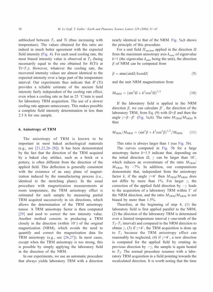
nearly identical to that of the NRM. Fig. 5a,b shows

the principle of this procedure.

For a unit field Hancient applied in the direction Xfrom the maximum anisotropy axis kmax of eigenvalue

kN1 (the eigenvalue kmin being the unit), the direction

b of NRM can be computed from

b ¼ atan sinX=kcosXð Þ ð9Þ

and the unit NRM magnetization from

MNRM ¼ ðsin2X þ k2cos2XÞ1=2 ð10Þ

If the laboratory field is applied in the NRM

direction b, we can calculate bV, the direction of the

laboratory TRM, from Eq. (9) with X=b and then the

angle c=b�bV (Fig. 5a,b). The ratio MTRM/MNRM is

thus

MTRM=MNRM ¼ ðsin2b þ k2cos2bÞ1=2=MNRM ð11Þ

This ratio is always larger than 1 (see Fig. 5b).

The curves computed in Fig. 5b for a large

anisotropy factor k=1.5 indicate that, depending on

the initial direction X, c can be larger than 108,which induces an overestimate of the ratio MTRM/

MNRM by ~7%. In addition, our computations

demonstrate that, independent from the anisotropy

factor k, if the angle cb48 then MTRM/MNRM does

not differ by more than 1%. For larger c, the

correction of the applied field direction by �c leads

to the acquisition of a laboratory TRM within 38 of

the NRM direction, and the ratio MTRM/MNRM is not

biased by more than 1.5%.

Therefore, at the beginning of step 4, (1) the

laboratory field is first applied parallel to the NRM,

(2) the direction of the laboratory TRM is determined

over a limited temperature interval (~one-tenth of the

T2–T1 interval) and compared to the NRM direction to

obtain c, (3) if cb48, the TRM acquisition is done up

to T1 because the TRM anisotropy effect can

reasonably be neglected, (4) if cN48, a new direction

is computed for the applied field by rotating its

previous direction by �c, the sample is again heated

to T2. The normal procedure resumes with a labo-

ratory TRM acquisition in a field pointing towards the

recalculated direction. It is worth noting that the time

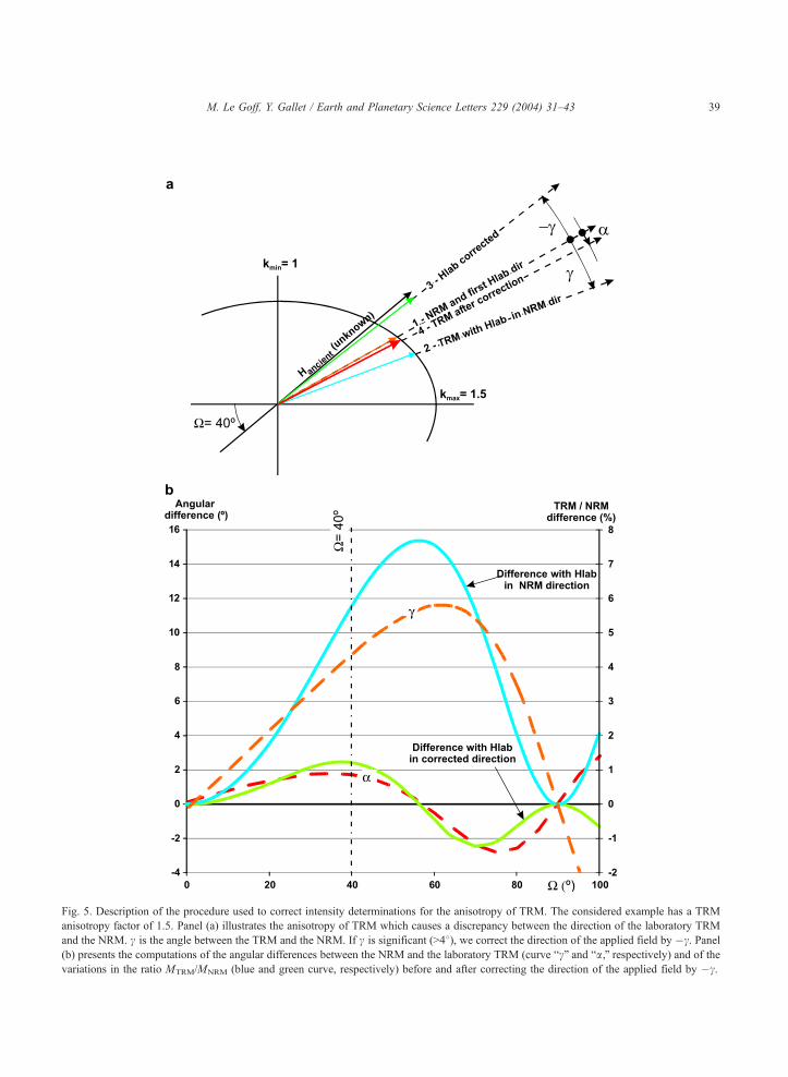
Fig. 5. Description of the procedure used to correct intensity determinations for the anisotropy of TRM. The considered example has a TRM

anisotropy factor of 1.5. Panel (a) illustrates the anisotropy of TRM which causes a discrepancy between the direction of the laboratory TRM

and the NRM. c is the angle between the TRM and the NRM. If c is significant (N48), we correct the direction of the applied field by �c. Panel(b) presents the computations of the angular differences between the NRM and the laboratory TRM (curve bcQ and ba,Q respectively) and of the

variations in the ratio MTRM/MNRM (blue and green curve, respectively) before and after correcting the direction of the applied field by �c.


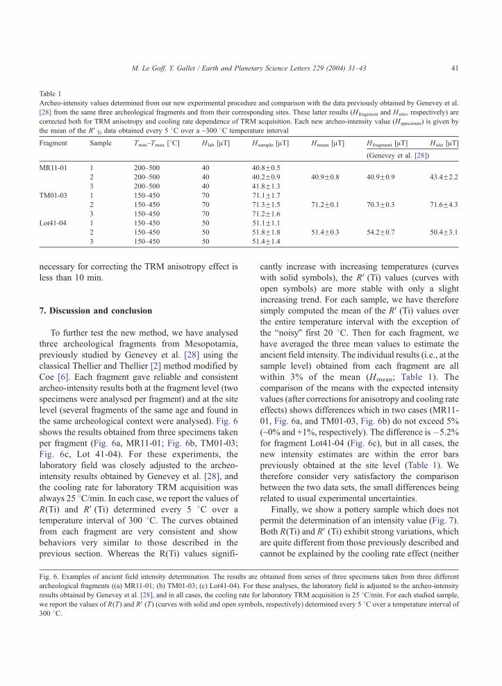
Table 1

Archeo-intensity values determined from our new experimental procedure and comparison with the data previously obtained by Genevey et al.

[28] from the same three archeological fragments and from their corresponding sites. These latter results (Hfragment and Hsite, respectively) are

corrected both for TRM anisotropy and cooling rate dependence of TRM acquisition. Each new archeo-intensity value (Hspecimen) is given by

the mean of the RVTi data obtained every 5 8C over a ~300 8C temperature interval

Fragment Sample Tmin–Tmax [8C] Hlab [AT] Hsample [AT] Hmean [AT] Hfragment [AT] Hsite [AT]

(Genevey et al. [28])

MR11-01 1 200–500 40 40.8F0.5

2 200–500 40 40.2F0.9 40.9F0.8 40.9F0.9 43.4F2.2

3 200–500 40 41.8F1.3

TM01-03 1 150–450 70 71.1F1.7

2 150–450 70 71.3F1.5 71.2F0.1 70.3F0.3 71.6F4.3

3 150–450 70 71.2F1.6

Lot41-04 1 150–450 50 51.1F1.1

2 150–450 50 51.8F1.8 51.4F0.3 54.2F0.7 50.4F3.1

3 150–450 50 51.4F1.4


necessary for correcting the TRM anisotropy effect is

less than 10 min.

7. Discussion and conclusion

To further test the new method, we have analysed

three archeological fragments from Mesopotamia,

previously studied by Genevey et al. [28] using the

classical Thellier and Thellier [2] method modified by

Coe [6]. Each fragment gave reliable and consistent

archeo-intensity results both at the fragment level (two

specimens were analysed per fragment) and at the site

level (several fragments of the same age and found in

the same archeological context were analysed). Fig. 6

shows the results obtained from three specimens taken

per fragment (Fig. 6a, MR11-01; Fig. 6b, TM01-03;

Fig. 6c, Lot 41-04). For these experiments, the

laboratory field was closely adjusted to the archeo-

intensity results obtained by Genevey et al. [28], and

the cooling rate for laboratory TRM acquisition was

always 25 8C/min. In each case, we report the values of

R(Ti) and RV(Ti) determined every 5 8C over a

temperature interval of 300 8C. The curves obtained

from each fragment are very consistent and show

behaviors very similar to those described in the

previous section. Whereas the R(Ti) values signifi-

Fig. 6. Examples of ancient field intensity determination. The results are

archeological fragments ((a) MR11-01; (b) TM01-03; (c) Lot41-04). For th

results obtained by Genevey et al. [28], and in all cases, the cooling rate fo

we report the values of R(T) and RV(T) (curves with solid and open symbol

300 8C.

cantly increase with increasing temperatures (curves

with solid symbols), the RV(Ti) values (curves with

open symbols) are more stable with only a slight

increasing trend. For each sample, we have therefore

simply computed the mean of the RV(Ti) values overthe entire temperature interval with the exception of

the bnoisyQ first 20 8C. Then for each fragment, we

have averaged the three mean values to estimate the

ancient field intensity. The individual results (i.e., at the

sample level) obtained from each fragment are all

within 3% of the mean (Hmean; Table 1). The

comparison of the means with the expected intensity

values (after corrections for anisotropy and cooling rate

effects) shows differences which in two cases (MR11-

01, Fig. 6a, and TM01-03, Fig. 6b) do not exceed 5%

(~0% and +1%, respectively). The difference is�5.2%

for fragment Lot41-04 (Fig. 6c), but in all cases, the

new intensity estimates are within the error bars

previously obtained at the site level (Table 1). We

therefore consider very satisfactory the comparison

between the two data sets, the small differences being

related to usual experimental uncertainties.

Finally, we show a pottery sample which does not

permit the determination of an intensity value (Fig. 7).

Both R(Ti) and RV(Ti) exhibit strong variations, whichare quite different from those previously described and

cannot be explained by the cooling rate effect (neither

obtained from series of three specimens taken from three different

ese analyses, the laboratory field is adjusted to the archeo-intensity

r laboratory TRM acquisition is 25 8C/min. For each studied sample,

s, respectively) determined every 5 8C over a temperature interval of

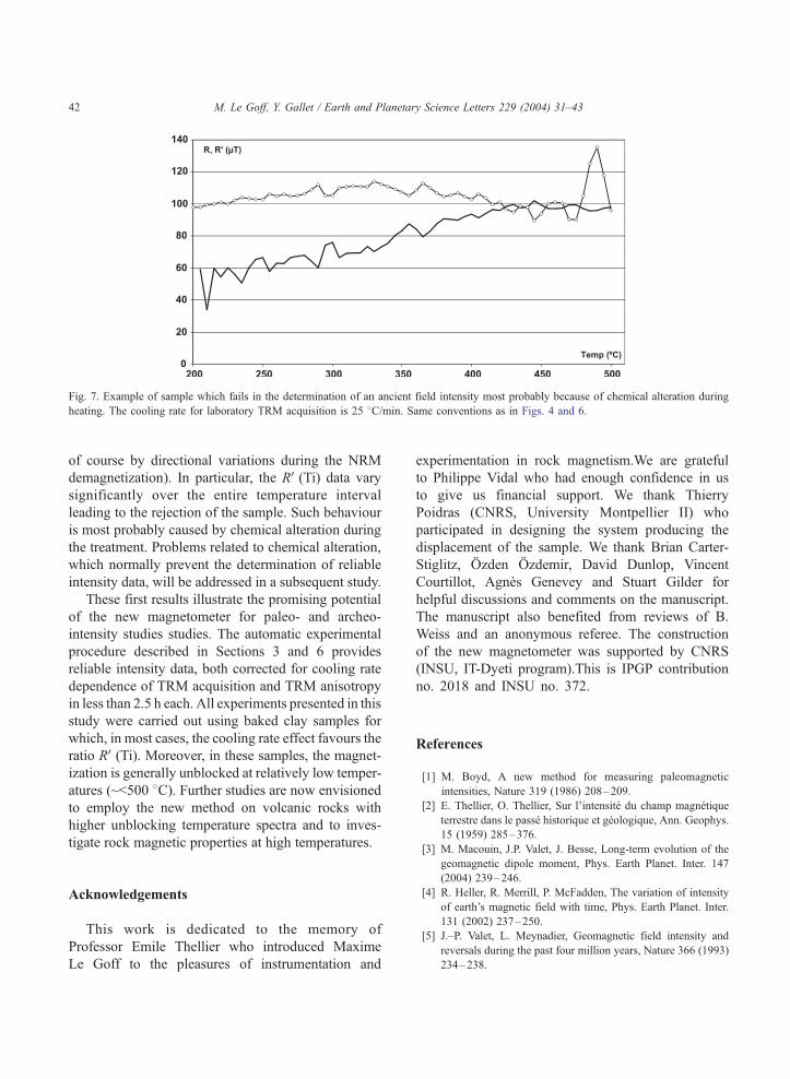
Fig. 7. Example of sample which fails in the determination of an ancient field intensity most probably because of chemical alteration during

heating. The cooling rate for laboratory TRM acquisition is 25 8C/min. Same conventions as in Figs. 4 and 6.


of course by directional variations during the NRM

demagnetization). In particular, the RV(Ti) data vary

significantly over the entire temperature interval

leading to the rejection of the sample. Such behaviour

is most probably caused by chemical alteration during

the treatment. Problems related to chemical alteration,

which normally prevent the determination of reliable

intensity data, will be addressed in a subsequent study.

These first results illustrate the promising potential

of the new magnetometer for paleo- and archeo-

intensity studies studies. The automatic experimental

procedure described in Sections 3 and 6 provides

reliable intensity data, both corrected for cooling rate

dependence of TRM acquisition and TRM anisotropy

in less than 2.5 h each. All experiments presented in this

study were carried out using baked clay samples for

which, in most cases, the cooling rate effect favours the

ratio RV(Ti). Moreover, in these samples, the magnet-

ization is generally unblocked at relatively low temper-

atures (~b500 8C). Further studies are now envisioned

to employ the new method on volcanic rocks with

higher unblocking temperature spectra and to inves-

tigate rock magnetic properties at high temperatures.

Acknowledgements

This work is dedicated to the memory of

Professor Emile Thellier who introduced Maxime

Le Goff to the pleasures of instrumentation and

experimentation in rock magnetism.We are grateful

to Philippe Vidal who had enough confidence in us

to give us financial support. We thank Thierry

Poidras (CNRS, University Montpellier II) who

participated in designing the system producing the

displacement of the sample. We thank Brian Carter-

Stiglitz, Ozden Ozdemir, David Dunlop, Vincent

Courtillot, Agnes Genevey and Stuart Gilder for

helpful discussions and comments on the manuscript.

The manuscript also benefited from reviews of B.

Weiss and an anonymous referee. The construction

of the new magnetometer was supported by CNRS

(INSU, IT-Dyeti program).This is IPGP contribution

no. 2018 and INSU no. 372.

References

[1] M. Boyd, A new method for measuring paleomagnetic

intensities, Nature 319 (1986) 208–209.

[2] E. Thellier, O. Thellier, Sur l’intensite du champ magnetique

terrestre dans le passe historique et geologique, Ann. Geophys.

15 (1959) 285–376.

[3] M. Macouin, J.P. Valet, J. Besse, Long-term evolution of the

geomagnetic dipole moment, Phys. Earth Planet. Inter. 147

(2004) 239–246.

[4] R. Heller, R. Merrill, P. McFadden, The variation of intensity

of earth’s magnetic field with time, Phys. Earth Planet. Inter.

131 (2002) 237–250.

[5] J.–P. Valet, L. Meynadier, Geomagnetic field intensity and

reversals during the past four million years, Nature 366 (1993)

234–238.


[6] R. Coe, Paleo-intensities of the earth’s magnetic field

determined from Tertiary and Quaternary rocks, J. Geophys.

Res. 72 (1967) 3247–3262.

[7] J. Shaw, A new method of determining the magnitude of the

paleomagnetic field, Geophys. J. R. Astron. Soc. 39 (1974)

133–141.

[8] J. Morales, A. Gogichaishvili, J. Urrutia, An experimental

evaluation of Shaw’s paleointensity method and its modifica-

tions using late Quaternary basalts, Geophys. Res. Abstr. 5

(2003) 01479.

[9] D. Walton, J. Shaw, J. Share, J. Hakes, Microwave demagnet-

ization, J. Appl. Phys. 71 (1992) 1549–1551.

[10] D. Walton, J. Share, T. Rolph, J. Shaw, Microwave magnet-

isation, Geophys. Res. Lett. 20 (1993) 109–111.

[11] J. Shaw, S. Yang, T. Rolph, F. Sun, A comparison of

archaeointensity results from Chinese ceramics using micro-

wave and conventional Thellier’s and Shaw’s methods, Geo-

phys. J. Int. 136 (1999) 714–718.

[12] L. Neel, Some theoretical aspects of rock magnetism, Adv.

Phys. 4 (1955) 191–243.

[13] K. Burakov, I. Nachasova, A method and results of studying

the geomagnetic field of Khiva from the middle of the

sixteenth century, Izv. Earth Phys. 14 (1978) 833–838.

[14] D. Walton, Re-evaluation of Greek archaeomagnitudes, Nature

310 (1984) 740–743.

[15] P. Schmidt, D. Clark, Step-wise and continuous thermal

demagnetization and theories of thermoremanence, Geophys.

J. R. Astron. Soc. 83 (1985) 731–751.

[16] N. Sigiura, Measurements of magnetization at high temper-

atures and the origin of thermoremanent magnetization: a

review, J. Geomagn. Geoelectr. 43 (1989) 3–17.

[17] H. Tanaka, J. Athanassopoulos, J. Dunn, M. Fuller, Paleo-

intensity determinations with measurements at high temper-

ature, J. Geomagn. Geoelectr. 47 (1995) 103–113.

[18] S. Levi, The effect of magnetite particle size on paleointensity

determination of the geomagnetic field, Phys. Earth Planet.

Inter. 13 (1977) 245–259.

[19] D. Walton, Archaeomagnetic intensity measurements using a

SQUID magnetometer, Archaeometry 19 (1977) 192–200.

[20] H. Tanaka, M. Kono, Analysis of the Thellier’s method of

paleointensity determination: 2. Application to high and

low magnetic fields, J. Geomagn. Geoelectr. 36 (1984)

285–297.

[21] A. Genevey, Y. Gallet, Intensity of the geomagnetic field in

Western Europe over the past 2000 years: new data from

French ancient pottery, J. Geophys. Res. 107 (2002) 2285.

[22] A. Chauvin, Y. Garcia, P. Lanos, F. Laubenheimer, Paleo-

intensity of the geomagnetic field recovered on archaeomag-

netic sites from France, Phys. Earth Planet. Inter. 120 (2000)

111–136.

[23] J. Fox, M. Aitken, Cooling-rate dependence of thermorema-

nent magnetization, Nature 283 (1980) 462–463.

[24] M. Dodson, E. McClelland-Brown, Magnetic blocking tem-

peratures of single-domain grains during slow cooling,

J. Geophys. Res. 85 (1980) 2625–2637.

[25] S. Halgedahl, R. Day, M. Fuller, The effect of cooling rate on

the intensity of weak-field TRM in single-domain magnetite,

J. Geophys. Res. 85 (1980) 3690–3698.

[26] J. Rogers, J. Fox, M. Aitken, Magnetic anisotropy in ancient

pottery, Nature 277 (1979) 644–646.

[27] M. Aitken, P. Alcock, G. Bussel, C. Shaw, Archaeomagnetic

determination of the past geomagnetic intensity using ancient

ceramics: allowance for anisotropy, Archaeometry 23 (1981)

53–64.

[28] A. Genevey, Y. Gallet, J. Margueron, Eight thousand years of

geomagnetic field intensity variations in the eastern Medi-

terranean, J. Geophys. Res. 108 (2003) 2228.

[29] R. Veitch, I. Hedley, J. Wagner, An investigation of the

intensity of the geomagnetic field during Roman times using

magnetically anisotropic bricks and tiles, Arch. Sci. 37 (1984)

359–373.

a new three-axis vibrating sample magnetometer for

Documents