a new method to synthesize a shock response …
TRANSCRIPT
A NEW METHOD TO SYNTHESIZE A SHOCK RESPONSE SPECTRUM
COMPATIBLE BASE ACCELERATION TO IMPROVE MULTI-DEGREE OF
FREEDOM SYSTEM RESPONSE
A DISSERTATION
SUBMITTED TO THE FACULTY OF THE
UNIVERSITY OF MINNESOTA
BY
J. EDWARD ALEXANDER
IN PARTIAL FULFILLMENT OF THE REQUIREMENTS
FOR THE DEGREE OF
DOCTOR OF PHILOSOPHY
PROFESSOR SUSAN C. MANTELL
NOVEMBER 2015

Copyright 2015 by
J. Edward Alexander
All Rights Reserved

i
Acknowledgements
I would like to acknowledge my advisor, Dr. Susan C. Mantell, for accepting me
back as a PhD student after a long haitus in my program due to personal reasons. Her
interest, advice, guidance and friendship have been much appreciated. I also would like
to thank the other members of my dissertation committee, Dr. William Durfee, Dr.
Rajesh Rajamani and Dr. Henryk Stolarski for their interest, questions, suggestions and
insightful comments.
ii
Dedication
This document is dedicated to Dr. Rudolph Scavuzzo, Dr. Howard Gaberson and
Mr. Henry Pusey. These three individuals all played key roles in the field of shock and
vibration over the course of their lives and are universally recognized as subject matter
experts in their respective areas of research and leadership.
Dr. Rudolph (Rudy) J. Scavuzzo is a consultant, ASME Fellow and Professor
Emeritis, Department of Polymer Engineering, University of Akron. Rudy was one of
the original developers of the Practical Naval Shock Analysis and Design short course.
Rudy and I both worked at Bettis Atomic Power Laboratory in Pittsburgh, however not at
the same time. Rudy handed the torch to me to continue teaching his material for the
naval shock course when he was physically no longer able to travel.
Dr. Howard (Howie) A. Gaberson (1931-2013) was the Division Director of the
U. S. Naval Civil Engineering Laboratory which later became the Facilities Engineering
Service Center. After retirement from government service, Howie continued research on
the pseudo-velocity shock spectrum. During his long career, Howie was an enthusiac
advocate for the pseudo-velocity shock spectrum as the best indicator of system damage.
Howie preeched the pseudo-velocity shock spectrum gospel for decades. Howie asked
me to continue his life-long mission for advocating the merits of the pseudo-velocity
shock spectrum.
Mr. Henry C. Pusey (1927 – 2014) is frequently referred to as the “Godfather” of
shock and vibration. Henry was the fourth and final Director of the Shock and Vibration
Information Center, Naval Reseach Laboratory. Henry was my friend and mentor for
more than three decades, and was instrumental in including me as an instructor in the
Practical Naval Shock Analysis and Design course, as well as numerous panels and
meetings. Henry was a true southern gentleman.
These three gentlemen provided not only guidance to me, but also to hundreds of
other engineers in the field of shock and vibration. They were my inspiration, mentors
and role models. I owe a debt of gratitude to all, and miss Howie and Henry greatly.
iii
Abstract
A new method has been developed to synthesize a shock response spectrum (SRS)
compatible base acceleration with additional parameters in the synthesis process beyond
current practices. Current base acceleration synthesis methods address only SRS
compatibility. However, additional information is available to synthesize a base
acceleration to improve multi-degree of freedom (MDOF) system response accuracy.
Expanding the synthesis procedure to include energy input and temporal information
provides more constraints on the development of the synthesized acceleration. Similar to
the SRS, an energy input spectrum (EIS) is a frequency based relationship for the peak
energy input per unit mass to a series of single-degree of freedom (SDOF) oscillators
from a base acceleration. The EIS represents total input energy contributions (kinetic,
damped and absorbed energy). Temporal information includes overall shape of the
transient shock pulse envelope E(t) (rise, plateau, decay) and a TE duration where strong
shock occurs. When EIS, E(t) and TE compatibility are added to the synthesis procedure,
an improved base acceleration results. To quantify the significance of these quantities, a
regression analysis was performed based on linear and nonlinear 3DOF model responses.
The regression analysis confirmed that compatibility with SRS, EIS and TE were
significant factors for accurate MDOF model response. To test this finding, a base
acceleration was synthesized with the expanded procedure. Four other accelerations were
synthesized with current state of the art methods which match the SRS only. The five
synthesized accelerations were applied to a 3DOF model based on a US naval medium
weight shock machine (MWSM). MWSM model results confirmed that the SRS, EIS, TE
compatible acceleration resulted in improved accuracy of peak mass accelerations and

iv
displacements in the majority of the cases, and consistently gave more accurate peak
energy input to the MWSM model. Energy input to a structure is a significant factor for
damage potential. The total kinetic, damped and absorbed energy input represents a
system damage potential which the structure as a whole must dissipate.
v
Table of Contents
List of Tables……………………………………………………………………………vii
List of Figures……………………………………………………………...………..…viii
Nomenclature………………………………………………………………….……..…..x
1 Spectral Methods to Characterize Shock and Energy ........................................... 1
1.1 Overview .............................................................................................................. 1
1.2 Shock Response Spectrum Definition .................................................................. 3
1.3 Shock Response Spectrum SRSD as a Shock Design Specification ..................... 6
1.4 Role of a Synthesized Acceleration ................................................................... 11
1.5 Research Objectives ........................................................................................... 13
1.6 Thesis Outline .................................................................................................... 13
1.7 Overview of Findings ......................................................................................... 15
2 Background .............................................................................................................. 16
2.1 Overview ............................................................................................................ 16
2.2 Derivation of the Shock Response Spectrum ..................................................... 16
2.3 Methods to Synthesize SRS Compatible Acceleration ....................................... 20
2.4 Evolution of Energy Methods for Shock and Vibration .................................... 31
2.5 Derivation of the Energy Input Equations.......................................................... 36
2.6 Temporal Information from a Shock Acceleration ............................................ 42
2.7 Define Baseline aD, SRSD, EISD and TED for Present Study ............................... 44
3 New Approach to Synthesize SRS Compatible Acceleration .............................. 46
3.1 Overview ............................................................................................................ 46
3.2 Traditional Synthesize Methods of SRSD Compatible Base Acceleration ......... 46
3.3 Synthesis of Base Acceleration aS ...................................................................... 47
3.4 Evaluate aS from MDOF Model Response ........................................................ 51
3.5 Determine Significant Factors and Merit Function from Regression Analysis . 55
3.6 Final as2 from Revised Merit Function .............................................................. 61
4 Multi-degree of Freedom Response to Synthesized Accelerations ..................... 64
4.1 Overview ............................................................................................................ 64
4.2 Synthesized Accelerations Evaluated................................................................. 64
vi
4.3 3DOF Medium Weight Shock Machine Model ................................................. 66
4.4 MWSM Model Response to Synthesized Accelerations ..................................... 68
5 Conclusions and Recommendations ...................................................................... 72
6 Bibliography ............................................................................................................. 75
Appendices:
A SRS and Mode Superposition ............................................................................. 81
B General 3DOF Model......................................................................................... 85
C Medium Weight Shock Machine 3DOF Model ................................................. 89
D Regression Analysis ........................................................................................... 93
vii
List of Tables
Table (2-1) Synthesized Accelerations SRSS % Error....................................................... 30
Table (3-1) Synthesized Acceleration Nomenclature base on M Weighting .................... 56
Table (3-2) Regression Analysis Input (Factors) and Output (Linear 3DOF Model
Responses) ........................................................................................................................ 58
Table (3-3) General 3DOF Model – Linear - Significant Factors .................................... 60
Table (3-4) General 3DOF Model, Nonlinear Stiffening – Significant Factors ............... 60
Table (3-5) General 3DOF Model, Nonlinear Softening – Significant Factors ............... 61
Table (4-1) Percent Errors of Synthesized Accelerations ................................................. 66
Table (B-1) Properties of Linear General 3DOF Model………………………….……..86
Table (B-2) Natural Frequencies of Linear General 3DOF Model……………………...86
Table (B-3) Linear Limits for Springs 1, 2 and 3………………………………………..88
Table (C-1) MWSM Linear Model Parameters…………………………………………..91
Table (C-2) MWSM Nonlinear Spring 2 Stiffness Values………………………………92
Table (D-1) General 3DOF Model, Linear – Significant Factors………………………..94
Table (D-2) General 3DOF Model, Nonlinear Stiffening – Significant Factors………...97
Table (D-3) General 3DOF Model, Nonlinear Softening – Significant Factors………...98
viii
List of Figures
Figure (1-1) Graphical Representation of the Shock Response Spectrum ......................... 5
Figure (1-2) Development of a Design SRSD from Field Test Data .................................... 7
Figure (1-3) U.S. NRC Horizontal SRSD for Nuclear Power Plants ................................... 8
Figure (1-4) MIL-STD-810G, Method 516, Functional and Crash Hazard Shock SRSD ... 9
Figure (1-5) MIL-STD-810G, Method 522, Ballistic Shock SRSD .................................. 10
Figure (1-6) MIL-STD-810G, Method 517, Pyrotechnic Devices SRSD .......................... 11
Figure (2-1) Series of SDOF Oscillators on a Common Base .......................................... 17
Figure (2-2) Typical Base Acceleration )(tub .................................................................. 17
Figure (2-3) Typical Shock Response Spectrum for Mechanical Shock .......................... 20
Figure (2-4) Individual Wavelet Example ........................................................................ 25
Figure (2-5) Individual Damped Sine Example ................................................................ 26
Figure (2-6) Envelope E(t) Superimposed on Corresponding Enveloped Sinusoids aS ... 27
Figure (2-7) Design aD and Synthesized Accelerations .................................................... 29
Figure (2-8) Design SRSD and SRSS of Synthesized Accelerations................................... 30
Figure (2-9) Transient Energy Input for 10 Hz SDOF ..................................................... 39
Figure (2-10) Base Acceleration )(tub Transient Energy Input for Three SDOF Oscillators
........................................................................................................................................... 40
Figure (2-11) Base Acceleration �̈�𝑏(𝑡)Energy Input Spectrum (EIS) .............................. 40
Figure (2-12) Shock Acceleration Envelope E(t) and Duration TE .................................. 43
Figure (2-13) Design Acceleration aD, Duration TED and Envelope E(t) ......................... 45
Figure (2-14) Design SRSD and EISD ................................................................................ 45
Figure (3-1) aS Synthesis Optimization Process ............................................................... 49
Figure (3-2) Process to Evaluate aS Accuracy .................................................................. 52
Figure (3-3) General 3DOF Model ................................................................................... 54
Figure (3-4) Eight aS Synthesized Accelerations .............................................................. 57
Figure (3-5) Synthesized Acceleration as2 ........................................................................ 62
Figure (3-6) SRSD and SRSs2 ............................................................................................. 63
Figure (3-7) EISD and EISs2 .............................................................................................. 63
Figure (4-1) Design Acceleration aD and Synthesized Accelerations .............................. 65
Figure (4-2) Illustration of Medium Weight Shock Machine ........................................... 67
Figure (4-3) 3DOF Model of Medium Weight Shock Machine ....................................... 67
Figure (4-4) Synthesized Accelerations Response % Error – MWSM Linear Model ....... 70
Figure (4-5) Synthesized Accelerations Response % Error – MWMS NL Stiffening Model
........................................................................................................................................... 71
Figure (4-6) Synthesized Accelerations Response % Error - MWSM NL-Softening Model
........................................................................................................................................... 71
Figure (B-1) General 3DOF Model………………………………………………….…..85
Figure (B-2) Force – Displacement Relationship Linear Spring………………………86
ix
Figure (B-3) Force – Displacement Relationship Nonlinear Elastic Stiffening Spring…….
……………………………………………………………………………………………87
Figure (B-4) Force – Displacement Relationship Nonlinear Elastic Softening
Spring…………………………………………………………………………………….87
Figure (C-1) Schematic of MIL-S-901D Medium Weigh Shock Machine……………...89
Figure (C-2) 3DOF Model of the Medium Weight Shock Machine…………………….90
Figure (C-3) Barry Controls SLM Series Shock Isolator………………………………..91
Figure (C-4) Force-Deflection Relationship of Barry Controls SLM-96 Shock Isolator..92
Figure (D-1) General 3DOF Model – Linear; Ave Peak Acceleration %Error; Regression
Equation & 3DOF Transient……………………………………………………………..95
Figure (D-2) General 3DOF Model – Linear; Ave z-Displacement %Error; Regression
Equation & 3DOF Transient……………………………………………………………..96
Figure (D-3) General 3DOF Model – Linear; Peak Energy Input %Error; Regression
Equation & 3DOF Transient……………………………………………………………..96

x
Nomenclature
3DOF Three degree of freedom
aD Design acceleration
aS Synthesized acceleration
aS2 Final synthesized acceleration from updated merit function
An Amplitude of nth
sinusoid
EI Energy input
EIS Energy input spectrum
EISD Energy input spectrum for aD
EISS Energy input spectrum for aS
EISS2 Energy input spectrum for aS2
EIS% EIS percent error of aS relative to aD averaged over frequency bandwidth
En Total peak energy input to MDOF model
EOM Equation of motion
E(t) Envelope function for synthesized acceleration
f Frequency, Hz
fn Natural frequency of nth
SDOF oscillator, Hz
g Acceleration due to gravity
H0 Null hypothesis in regression analysis
H1 Alternative hypothesis in regression analysis
HV Velocity transfer function
Hz Hertz (cycles/second)
i Iteration index for aS synthesis iteration process
ITOP International test operations procedure
j Index for jth
m, c and k in MDOF model
k Index for time step increment
kj jth
spring stiffness in MDOF model
KPH Kilometers per hour
M Merit function
m Mass
mj jth
mass in MDOF model
MDOF Multi-degree of freedom
MOD Ministry of Defense
MWSM Medium weight shock machine
Nn Number of half sines in nth
wavelet
n Frequency index
Pn Participation factor for nth
mode of vibration
PSD Power spectral density
R2 Percent that regression model explains the variation in response

xi
SDOF Single degree of freedom
SRS Shock response spectrum
SRSD Shock response spectrum for aD
SRSS Shock response spectrum for aS
SRSS2 Shock response spectrum for aS2
SRSvel Velocity SRS
SRS% SRS percent error of aS relative to aD averaged over frequency bandwidth
tdn Wavelet time delay
TE Temporal duration of acceleration time-history defined in Chapter 3.2
TED Temporal duration TE for aD
TES Temporal duration TE for aS
TE% TE percent error of aS relative to aD
u(t) Absolute acceleration
�̇�(𝑡) Absolute velocity
�̈�(𝑡) Absolute acceleration
�̈�𝑏(𝑡) Base acceleration
UK United Kingdom
WEIS EIS% weighting in merit function (M) equation
WSRS SRS% weighting in merit function (M) equation
WTE TE% weighting in merit function (M) equation
x Modal coordinate
�̇�(𝑡) Modal coordinate velocity
�̈�(𝑡) Modal coordinate acceleration
z(t) Relative displacement
�̇�(𝑡) Relative velocity
�̈�(𝑡) Relative acceleration
Greek Alphabet Nomenclature:
α Mass matrix coefficient for Raleigh damping
β Stiffness matrix coefficient for Raleigh damping
Δ Elastic limit for nonlinear-elastic springs in 3DOF models
ζ Percent of critical damping
φn Phase angle for nth
sinusoid
ωi Circular frequency for ith
mode of vibration, radians/second
ωn Natural frequency of nth
SDOF oscillator, radians/second
Matrix Nomenclature:
[C] Damping matrix
[CL] Linear part of damping matrix
xii
[CNL] Nonlinear part of damping matrix which is function of velocity
[K] Stiffness matrix
[KL] Linear part of stiffness matrix
[KNL] Nonlinear part of stiffness matrix which is function of displacement
[M] Mass matrix
{xi} Modal coordinate vector for mode i
{u} Absolute displacement vector
{z} Relative displacement vector
{�̈�} Relative acceleration vector
{φ}n Mode shape vector for mode n
[Φ] Mode transformation matrix
1
1 Spectral Methods to Characterize
Shock and Energy
1.1 Overview
The shock response spectrum (SRS), conceived by Maurice Biot (1932), has been
used as a structural dynamic method to characterize the seismic and mechanical shock
environment for more than eight decades. The SRS, by definition, is the peak
acceleration response of a series of single-degree of freedom (SDOF) mechanical
oscillators of different frequencies, all with same the percent of critical damping,
subjected to the same transient base input acceleration. The SRS is most frequently
presented as a log-log graph of the peak SDOF acceleration responses as a function of the
frequency bandwidth of interest. Early research and application of the SRS was
conducted in the 1950’s by the seismic community (Hudson, 1956), (Housner, 1959) to
characterize the earthquake seismic shock environment. After the 1950’s the use of the
SRS expanded significantly for the seismic, aerospace and defense communities. The SRS
is frequently employed to specify the design requirement for the structural dynamic shock
environment that a physical system must survive (Bureau of Ships, 1961), (Department of
Defense, 2008), (NASA, 1999), (NASA, 2001).
When structural dynamic requirements are specified in terms of a design shock
response spectrum, termed SRSD, the evaluation of a structure to meet this requirement
can be demonstrated by either analysis or test. If it can be demonstrated the structure will
survive the input shock specified by SRSD and continue to meet operational requirements,
2
it is considered to be shock qualified. When the system to be shock qualified can be
modelled as a linear structure (i.e., linear equations of motion), a mode superposition
analysis procedure can be performed directly, using SRSD, to estimate the peak dynamic
response (accelerations, displacements) of a multi-degree of freedom (MDOF) system.
However, if the structure is to be shock qualified by electro-dynamic shaker
testing, or if the structure to be analyzed is nonlinear (i.e., nonlinear equations of motion),
the SRSD cannot be used directly. In these instances an SRSD compatible acceleration
time-history, aS, must be synthesized. The synthesized aS can be input directly as a
transient base acceleration for transient analysis of the nonlinear MDOF model, or to
drive the armature of an electro-dynamic shock test machine.
Synthesis of an SRSD compatible base acceleration time-history is not difficult to
execute and numerous procedures have been documented for this purpose. However,
past research has demonstrated that synthesis of an SRSD compatible acceleration time-
history aS does not, by itself, guarantee that the peak dynamic structure responses will be
accurate. Accurate, in the context of this document, is defined as system response from a
synthesized base acceleration that matches the corresponding system response from a
design acceleration with good accuracy, for example within 10%. Current SRSD
compatible synthesis methods do not consider compatibility with the energy input
spectrum (EIS) nor the temporal shape of aS. Motivation for the research documented
herein is to augment existing SRSD compatible transient acceleration aS synthesis
processes to improve the accuracy of peak MDOF system response. Additional
constraints beyond only SRSD compatibility are:
3
Matching the energy input to the structure based on the synthesized
acceleration’s compatibility with the energy input spectrum (EIS) and,
Constraining the synthesized acceleration to match predefined temporal
requirements including the overall shape envelope of the transient acceleration
and the duration TE of strong shock as defined by Military Standard 801G
(Department of Defense, 2008).
1.2 Shock Response Spectrum Definition
Shock is a major structural design consideration for a wide variety of systems and
their components. Shock is a sudden, sometimes violent, change in velocity (rapid
acceleration) of a physical system due to the transient application of an external force or
acceleration. The shock response spectrum is a way to characterize the frequency
response of a series of single degree-of-freedom (SDOF) systems all subjected to the
same transient base input shock acceleration. The SRS has been used for more than 80
years to characterize the frequency response from transient shock acceleration. The SRS
is defined simply as the peak acceleration response (either positive or negative) of a
series of base excited linear SDOF oscillators of different frequencies subjected to the
same transient base acceleration input.
Figure (1-1) is a graphical representation of how an SRS is determined. Consider
a base transient shock input acceleration time-history where the entire base experiences
this acceleration. A series of SDOF linear oscillators of different frequencies mounted on
the rigid base will also experience this transient shock input. To illustrate the SRS, the
response of six SDOF oscillators is examined in this example. These SDOF oscillators

4
are tuned to frequencies of 30 Hz, 60 Hz, 200 Hz, 500 Hz, 1000Hz and 1300 Hz. The
transient mass acceleration response of each is plotted above the corresponding SDOF
oscillator and the peak value is indicated on each plot. For example, the peak
acceleration response of the 30 Hz SDOF oscillator is -10.46g as indicated on the plot,
which is the lowest magnitude of the six SDOF oscillators. The peak amplitude of the 60
Hz SDOF oscillator is 22.7g. The SDOF peak amplitudes continue to increase to 151.2g
for the 1300 Hz oscillator. Had higher frequency oscillators been included in this
example, at some SDOF frequency, the peak SDOF acceleration response value would
reach a maximum. For SDOF oscillators with frequencies above this limiting frequency,
the peak acceleration response would begin to decrease. In the limit, at the extreme high
frequency end of the spectrum, the peak amplitude of the highest frequency oscillator
would asymptotically converge to 47.5g, which is the peak amplitude of the input base
acceleration. This is because, at the high frequency end of the spectrum, the SDOF
oscillator is so stiff that it acts like a rigid (infinitely stiff) element attached to the base,
and as such experiences acceleration identical to that of the base input acceleration. The
SRS approaching the high frequency asymptote is demonstrated by the SRS of Figure (2-
3) in Chapter 2.
The peak acceleration response of each of the six SDOF oscillators is plotted as a
function of frequency at the top of Figure (1-1). These six points are indicated on the
SRS plot at the corresponding frequencies of each oscillator. It is noted that the peak
acceleration of each SDOF oscillator do not occur at the same point in time during the
transient. The SRS gives the peak response of each SDOF, but does not retain temporal
information as to when the peak occurs. The complete SRS is developed for SDOF
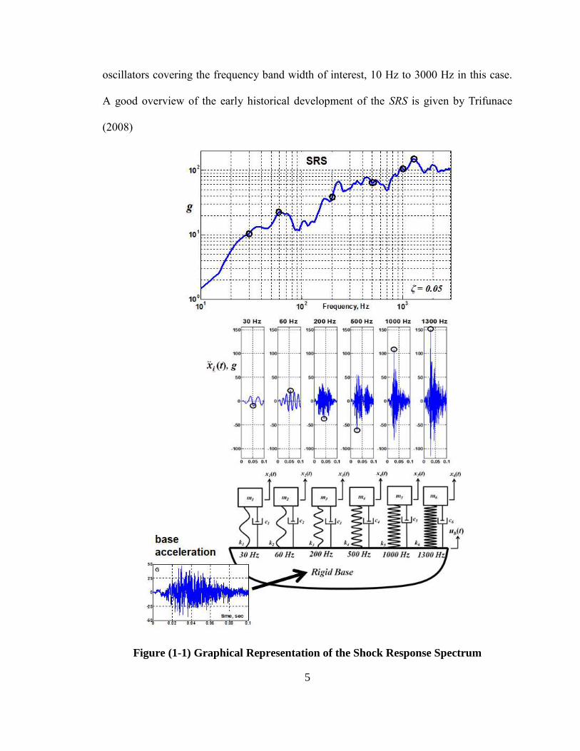
5
oscillators covering the frequency band width of interest, 10 Hz to 3000 Hz in this case.
A good overview of the early historical development of the SRS is given by Trifunace
(2008)
Figure (1-1) Graphical Representation of the Shock Response Spectrum
6
1.3 Shock Response Spectrum SRSD as a Shock Design
Specification
The SRS is used widely in the defense, aerospace and seismic communities. The
SRS is often prescribed as a structural design shock design specification, termed SRSD
herein, to characterize the requirement for the structural shock design environment. A
design shock response spectrum SRSD is frequently determined from platform (i.e., ship,
ground vehicle, etc.) field testing. In these cases, numerous transient accelerations data
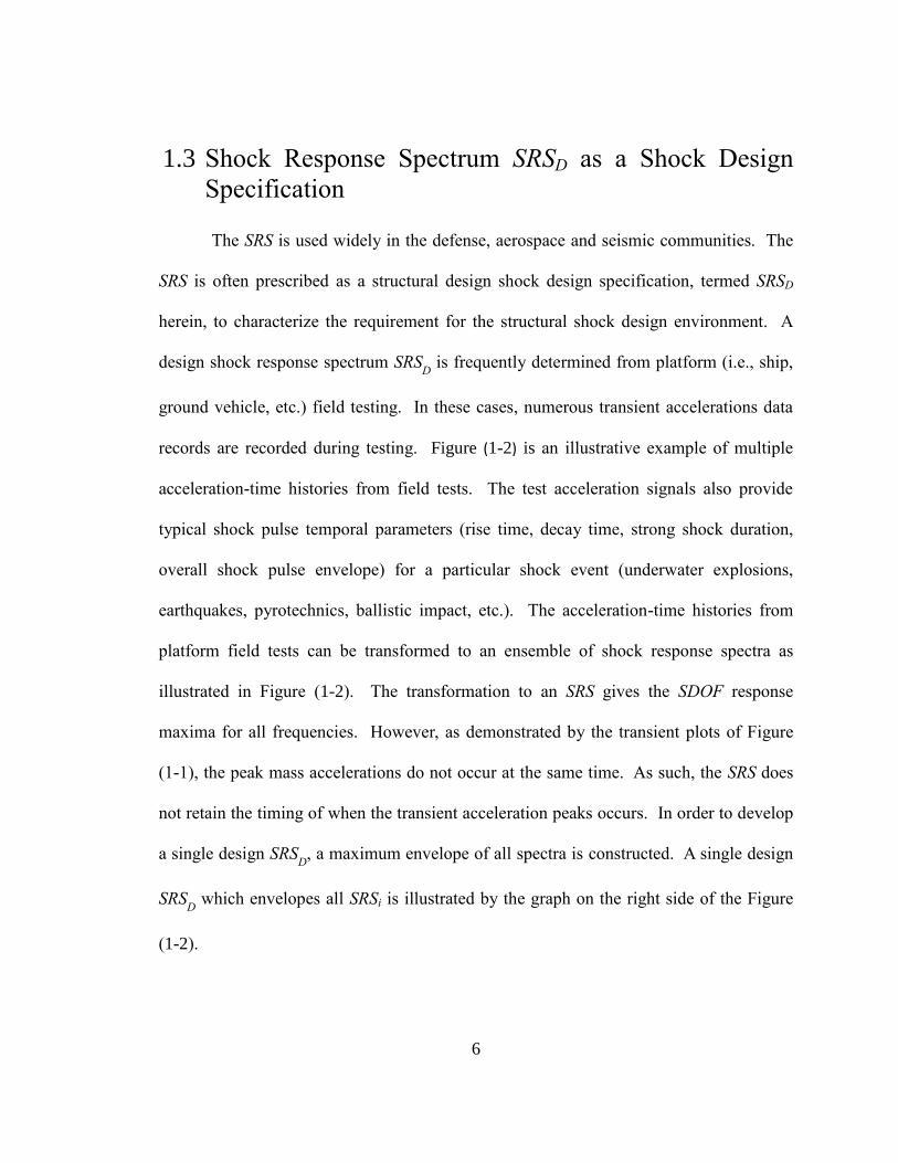
records are recorded during testing. Figure (1-2) is an illustrative example of multiple
acceleration-time histories from field tests. The test acceleration signals also provide
typical shock pulse temporal parameters (rise time, decay time, strong shock duration,
overall shock pulse envelope) for a particular shock event (underwater explosions,
earthquakes, pyrotechnics, ballistic impact, etc.). The acceleration-time histories from
platform field tests can be transformed to an ensemble of shock response spectra as
illustrated in Figure (1-2). The transformation to an SRS gives the SDOF response
maxima for all frequencies. However, as demonstrated by the transient plots of Figure
(1-1), the peak mass accelerations do not occur at the same time. As such, the SRS does
not retain the timing of when the transient acceleration peaks occurs. In order to develop
a single design SRSD, a maximum envelope of all spectra is constructed. A single design
SRSD which envelopes all SRSi is illustrated by the graph on the right side of the Figure
(1-2).
7
Figure (1-2) Development of a Design SRSD from Field Test Data
There are numerous examples where structural dynamic environment
requirements for a shock event are specified by a design SRSD. The seismic environment
for ground structures was the first case of this approach for design. Housner (1959)
published both velocity and acceleration spectra based on enveloping the four strongest
earthquake ground motions recorded at the time (El Centro-1934, El Centro-1940,
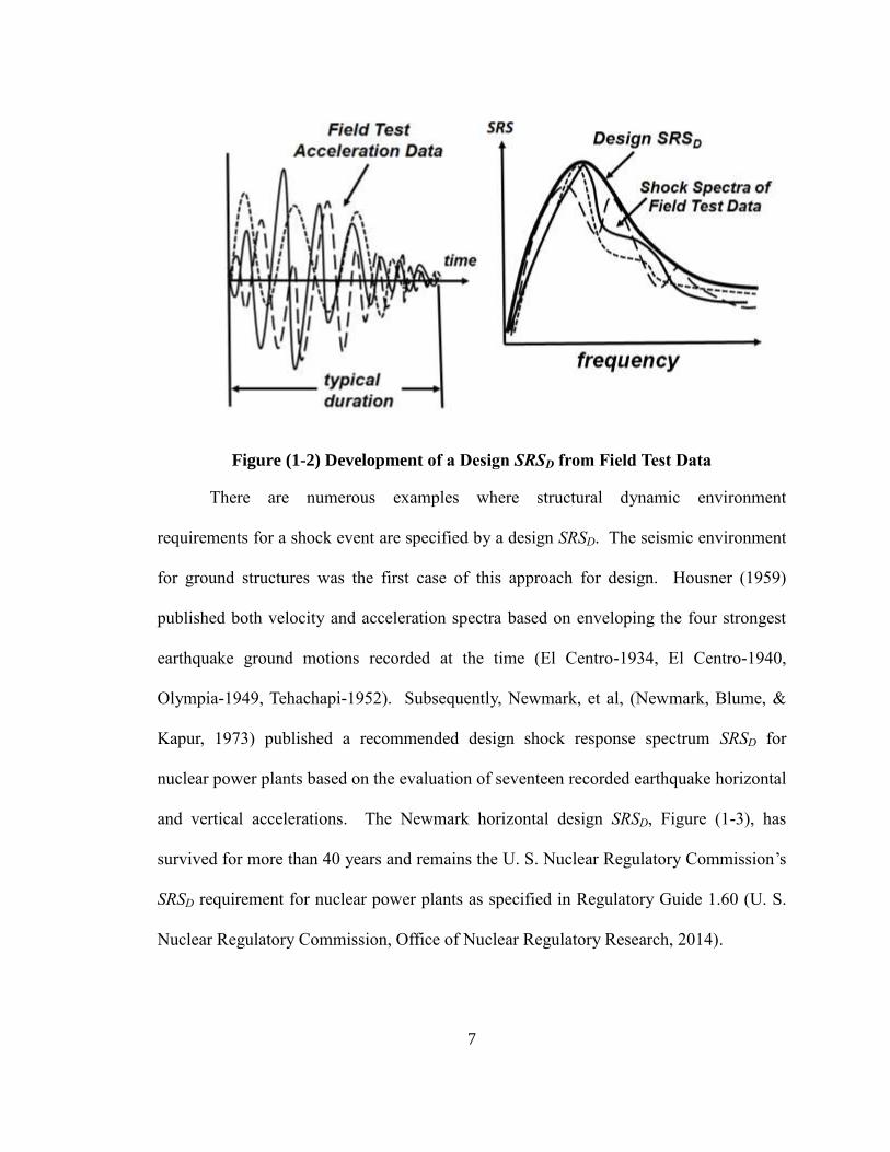
Olympia-1949, Tehachapi-1952). Subsequently, Newmark, et al, (Newmark, Blume, &
Kapur, 1973) published a recommended design shock response spectrum SRSD for
nuclear power plants based on the evaluation of seventeen recorded earthquake horizontal
and vertical accelerations. The Newmark horizontal design SRSD, Figure (1-3), has
survived for more than 40 years and remains the U. S. Nuclear Regulatory Commission’s
SRSD requirement for nuclear power plants as specified in Regulatory Guide 1.60 (U. S.
Nuclear Regulatory Commission, Office of Nuclear Regulatory Research, 2014).
8
Figure (1-3) U.S. NRC Horizontal SRSD for Nuclear Power Plants
Similar shock response spectrum requirements for equipment aboard US naval
ships were first published by the Naval Research Laboratory in 1963. In the case of
shipboard equipment, the design spectra is specified based on the type of ship (surface
ship or submarine) and the mounting location of the equipment in the ship, (hull, deck or
shell mounted). Interim unclassified design SRSD values were first published by Naval
Research Lab engineers O’Hara and Belsheim (Feb, 1963). Subsequently a classified
SRSD requirements document was issued by the US Navy (Department of the Navy,
Naval Sea Systems Command, 1972). This document remains the US Navy’s SRSD
requirement for shock qualification of naval equipment by analysis.
For other military equipment, MIL-STD-810G, Method 516, Shock (Department
of Defense, 2008) specifies requirements for a several shock qualification SRSD. If field
test data are available, the general 810G guidance is to determine SRSD with the
9
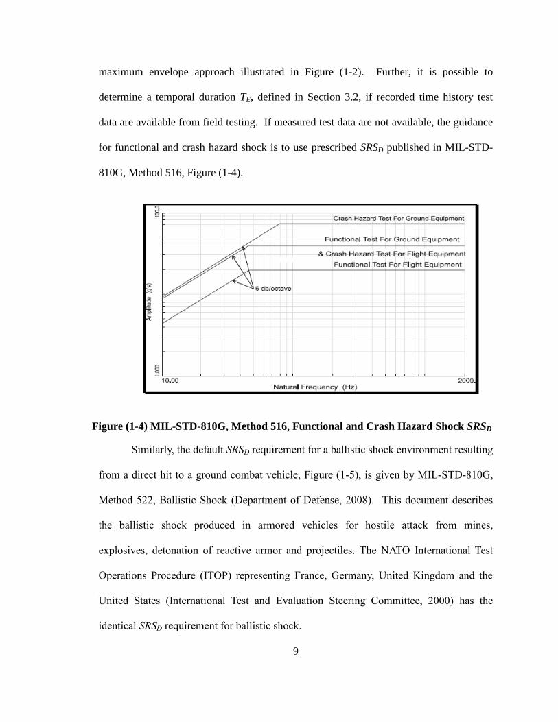
maximum envelope approach illustrated in Figure (1-2). Further, it is possible to
determine a temporal duration TE, defined in Section 3.2, if recorded time history test
data are available from field testing. If measured test data are not available, the guidance
for functional and crash hazard shock is to use prescribed SRSD published in MIL-STD-
810G, Method 516, Figure (1-4).
Figure (1-4) MIL-STD-810G, Method 516, Functional and Crash Hazard Shock SRSD
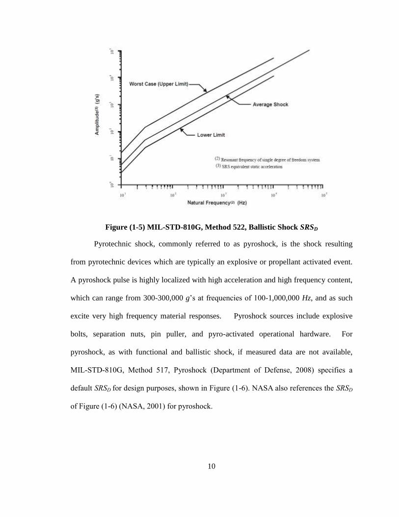
Similarly, the default SRSD requirement for a ballistic shock environment resulting
from a direct hit to a ground combat vehicle, Figure (1-5), is given by MIL-STD-810G,
Method 522, Ballistic Shock (Department of Defense, 2008). This document describes
the ballistic shock produced in armored vehicles for hostile attack from mines,
explosives, detonation of reactive armor and projectiles. The NATO International Test
Operations Procedure (ITOP) representing France, Germany, United Kingdom and the
United States (International Test and Evaluation Steering Committee, 2000) has the
identical SRSD requirement for ballistic shock.
10
Figure (1-5) MIL-STD-810G, Method 522, Ballistic Shock SRSD
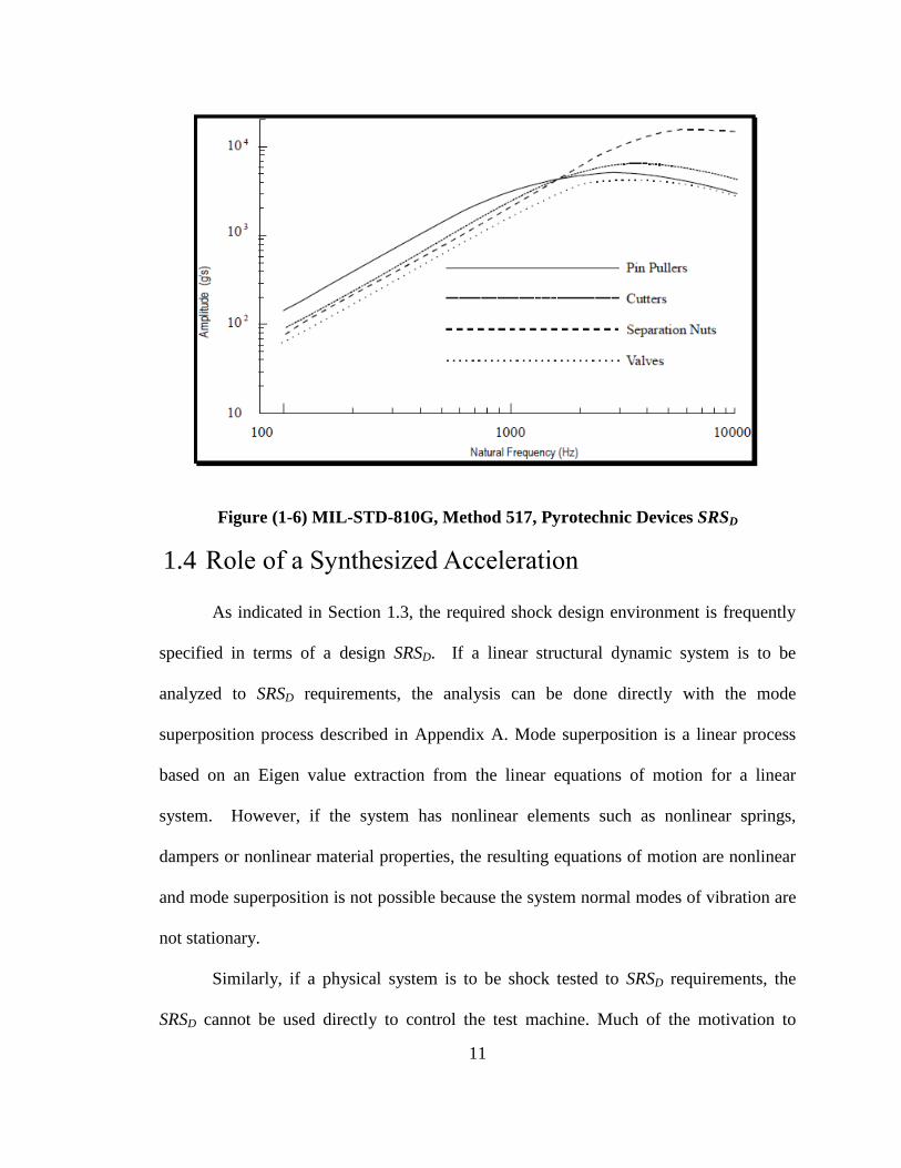
Pyrotechnic shock, commonly referred to as pyroshock, is the shock resulting
from pyrotechnic devices which are typically an explosive or propellant activated event.
A pyroshock pulse is highly localized with high acceleration and high frequency content,
which can range from 300-300,000 g’s at frequencies of 100-1,000,000 Hz, and as such
excite very high frequency material responses. Pyroshock sources include explosive
bolts, separation nuts, pin puller, and pyro-activated operational hardware. For
pyroshock, as with functional and ballistic shock, if measured data are not available,
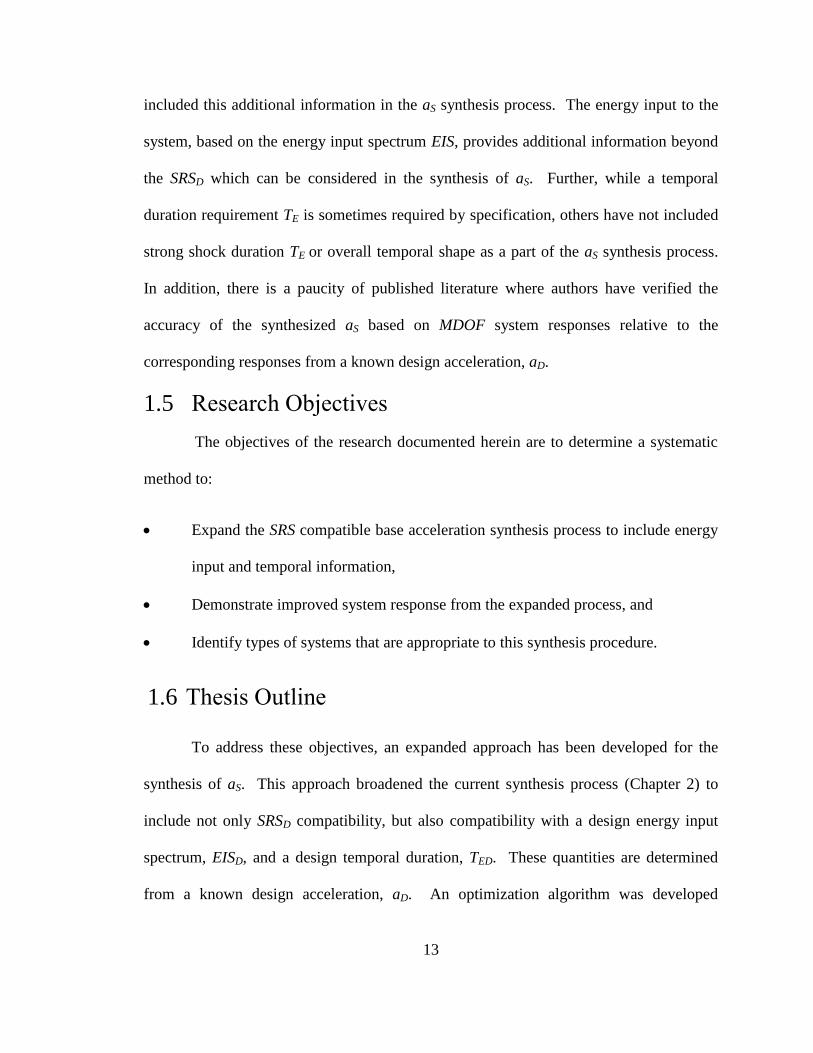
MIL-STD-810G, Method 517, Pyroshock (Department of Defense, 2008) specifies a
default SRSD for design purposes, shown in Figure (1-6). NASA also references the SRSD
of Figure (1-6) (NASA, 2001) for pyroshock.
11
Figure (1-6) MIL-STD-810G, Method 517, Pyrotechnic Devices SRSD
1.4 Role of a Synthesized Acceleration
As indicated in Section 1.3, the required shock design environment is frequently
specified in terms of a design SRSD. If a linear structural dynamic system is to be
analyzed to SRSD requirements, the analysis can be done directly with the mode
superposition process described in Appendix A. Mode superposition is a linear process
based on an Eigen value extraction from the linear equations of motion for a linear
system. However, if the system has nonlinear elements such as nonlinear springs,
dampers or nonlinear material properties, the resulting equations of motion are nonlinear
and mode superposition is not possible because the system normal modes of vibration are
not stationary.
Similarly, if a physical system is to be shock tested to SRSD requirements, the
SRSD cannot be used directly to control the test machine. Much of the motivation to

12
determine a synthesized aS compatible with a design SRSD is for shock testing with
electro-dynamic shakers (Smallwood & Nord, 1974) (Smallwood, 1986) (Nelson, 1989).
These types of test machines have physical limitations in terms of how much force they
can deliver to the test article and maximum displacement limitations of the shaker
armature. The peak shaker force is based on the peak acceleration of the transient
acceleration time-history and the weight of the equipment being tested (max force =
mass*peak acceleration). The peak displacement limitation can also be problematic for
low frequencies where the acceleration is generally low but the peak displacement is
high.
In both cases of analysis or test, a synthesized SRSD compatible shock
acceleration time-history, aS, is necessary. It is not difficult to synthesize a transient aS
with a corresponding SRSS that matches a prescribed SRSD within a specified tolerance
envelope requirement. Many techniques exist to synthesize a shock acceleration,
described in Section 2.3, based solely on matching the SRSD with no consideration of
other constraints. The assumption has been that if SRSS from aS matches SRSD within
prescribed tolerances, when aS is applied to a system model or test article by analysis or
test, respectively, the system response should be accurate. However, past studies have
demonstrated that system responses to a synthesized base acceleration aS can, and
frequently do, vary significantly from responses to the design acceleration aD. Additional
useful information is available to mitigate this problem. This information includes the
energy input to the structure from the shock acceleration and, if field test data are
available, temporal information for the overall shape envelope and temporal duration TE
of the shock acceleration. However, based on published literature, others have not
13
included this additional information in the aS synthesis process. The energy input to the
system, based on the energy input spectrum EIS, provides additional information beyond
the SRSD which can be considered in the synthesis of aS. Further, while a temporal
duration requirement TE is sometimes required by specification, others have not included
strong shock duration TE or overall temporal shape as a part of the aS synthesis process.
In addition, there is a paucity of published literature where authors have verified the
accuracy of the synthesized aS based on MDOF system responses relative to the
corresponding responses from a known design acceleration, aD.
1.5 Research Objectives
The objectives of the research documented herein are to determine a systematic
method to:
Expand the SRS compatible base acceleration synthesis process to include energy
input and temporal information,
Demonstrate improved system response from the expanded process, and
Identify types of systems that are appropriate to this synthesis procedure.
1.6 Thesis Outline
To address these objectives, an expanded approach has been developed for the
synthesis of aS. This approach broadened the current synthesis process (Chapter 2) to
include not only SRSD compatibility, but also compatibility with a design energy input
spectrum, EISD, and a design temporal duration, TED. These quantities are determined
from a known design acceleration, aD. An optimization algorithm was developed
14
(Chapter 3) to return aS which minimizes the following three factors with a merit function
M,
SRS% (average % error of SRSS:SRSD),
EIS% (average % error of EISS:EISD) and
TE% (average % error of TES:TED ).
A regression analysis was performed based on eight accelerations synthesized
with the merit function and the corresponding eight sets of 3DOF system responses.
Based on regression analysis, an updated merit function was formulated that included the
above three factors and also the products (or cross terms) of the factors. An optimized
acceleration aS2 was synthesized with the updated merit function.
The optimized aS2 was compared with four aS synthesized using common industry
practices (classical pulse, damped sines, wavelets, enveloped sines), (Chapter 4). To
evaluate the accuracy of the five aS, a second 3DOF model was developed based on the
U. S. Navy’s medium weight shock machine (MWSM). Representative linear and
nonlinear variants of the MWSM model were developed. MWSM model responses were
determined from the five aS. Responses evaluated were peak mass accelerations, peak
displacements and peak system energy input per unit mass. The peak model responses
from synthesized aS were compared with the corresponding MWSM model peak
responses from a prescribed design acceleration aD. The accuracy of each aS was
evaluated based on the MWSM model responses.

15
1.7 Overview of Findings
Evaluation of all aS was based on the peak responses of the MWSM 3DOF models
compared to the corresponding response from the design acceleration, aD. Three MWSM
model responses evaluated were;
Average % error of peak mass accelerations,
Average % error of peak mass displacements, and
% error of 3DOF peak energy input.
For the MWSM model linear variant, the optimized aS2 resulted in the lowest percent
errors for all three responses. For the two nonlinear MWSM variants, optimized aS2 had
lower percentage errors relative to the other four synthesized aS, for peak mass
accelerations and displacements in the majority of the cases. For all MWSM model
variants (linear and nonlinear), the optimized aS2 resulted in the lowest peak energy input
percent error. The optimized aS2 was the only synthesized shock acceleration that
included matching the energy input spectrum from the design acceleration, EISD, as a part
of the optimization process.
Energy input to a system from shock acceleration represents integrating the
energy equation over the entire structure, and as such is a comprehensive measure of total
system damage potential. On the other hand, local displacements and accelerations
cannot represent the damage potential for the entire structure and do not have general
significance for the entire structure.

16
2 Background
2.1 Overview
Numerous methods exist to synthesize a base acceleration aS to be compatible
with a design SRSD. Current practices focus on the singular goal of achieving the best
match of SRSS with SRSD. However, additional information is available to augment the
synthesis of aS including the energy input per unit mass, which can be derived from the
SRSD, and temporal information that can be extracted from available test data. An
overview of the common aS synthesis methods is described herein. Derivations of the
SRS and the energy input equations are presented. Temporal information is defined
including shock pulse durations and overall envelope.
2.2 Derivation of the Shock Response Spectrum
The SRS was defined and illustrated in Section 1.2 as the maximum response
acceleration from a series of linear SDOF oscillators covering a frequency range when
subjected to a common input base acceleration-time history. In this section the maximum
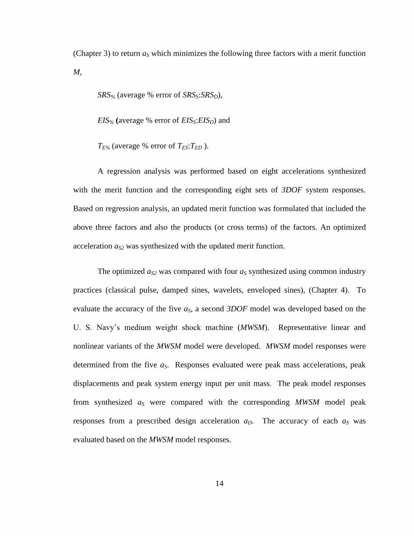
response of each SDOF oscillator of circular frequency ωn is derived. Consider a series
of linear damped SDOF oscillators with N different natural frequencies, all mounted on a
common fixed base, shown in Figure (2-1).
17
Figure (2-1) Series of SDOF Oscillators on a Common Base
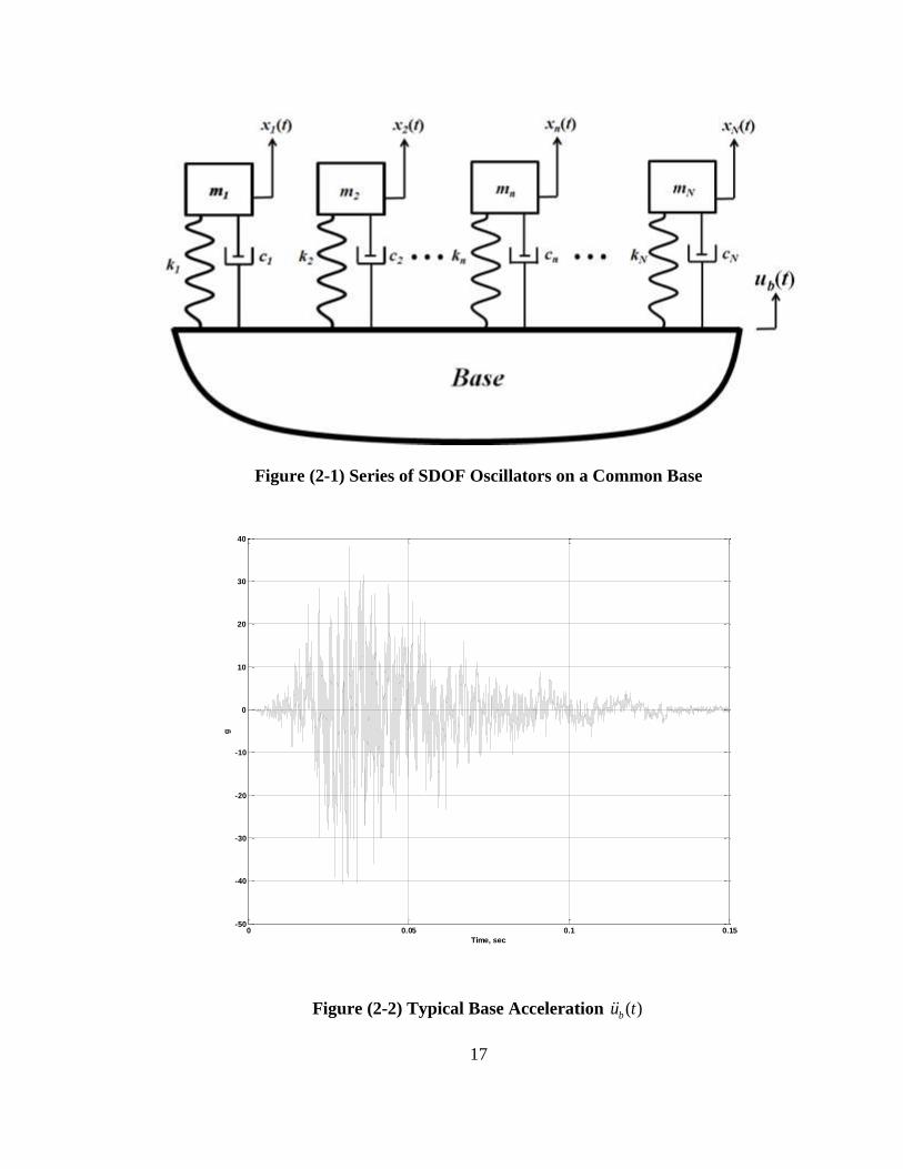
Figure (2-2) Typical Base Acceleration )(tub
0 0.05 0.1 0.15-50
-40
-30
-20
-10
0
10
20
30
40
Time, sec
g

18
Each oscillator has an independent absolute coordinate, )(txn . The base coordinate is
)(tub . If the base is subjected to transient shock acceleration )(tub such as the one shown
in Figure (2-2), this will induce an independent response in each oscillator. The
governing equation of motion for the nth
oscillator, developed by putting mn in dynamic
force equilibrium from d’Alembert’s principle, is
0)()()()()( tutxktutxctxm bnnbnnnn , (2-1)
where )(txn is an absolute coordinate for the displacement of the nth
mass nm . A
relative coordinate for the displacement of the mass relative to the base is defined for
each oscillator as,
)()()( tutxtz bnn . (2-2)
Substituting (2-2) into (2-1) yields,
0)()()()( tzktzctutzm nnnnbnn . (2-3)
Dividing by mn and moving the base acceleration base acceleration term to the right hand
side of the equation gives,
)()()()( tutzm
ktz
m
ctz bn
n
nn
n
nn
. (2-4)
It is recognized that 2
n
n
n
m
k is the squared natural frequency of the n
th oscillator and
that nn
n
n
m
c2 is the damping term where n is the percent of critical damping.
Making these substitutions gives a SDOF equation of motion (2-5) in relative coordinates
zn as,

19
)()()(2)( 2 tutztztz bnnnnnn . (2-5)
From (2-1), (2-2) and (2-4), the absolute acceleration of mass mn is determined from the
relative velocity and relative displacement given by equation (2-6),
)()(2)( 2 tztztx nnnnnn . (2-6)
The damping term is frequently ignored on the basis that the damping force contributes
little to the equilibrium relationship (Clough & Penzien, 1975), resulting in a relationship
between the absolute acceleration and the relative displacement,
)()( 2 tztx nnn . (2-7)
Equation (2-7) indicates that the absolute acceleration of the nth
mass is proportional to
the relative displacement between the mass and the base, with the proportionality being
the squared circular frequency. The solution to equation (2-5) is given by Duhamel’s
Integral,
dteutz n
tt
b
n
nnn )(1sin)(
1
1)( 2
0
)(
2
. (2-8)
Substituting (2-8) into (2-7) gives the absolute acceleration of mass mn, equation (2-9),
t
n
t
bn
n dteutx nn
0
2)(
2)(1sin)(
1)(
. (2-9)
The SRS defined as the absolute value of the peak mass accelerations over all frequencies
n . For the nth
frequency this is given by,
max
)(txSRS nn . (2-10)
Substitution of equation (2-9) into (2-10) gives the SRSn value for the nth
frequency
SDOF oscillator,
20
max
0
2)(
2)(1sin)(
1
t
n
t
bn
n dteuSRS nn
. (2-11)
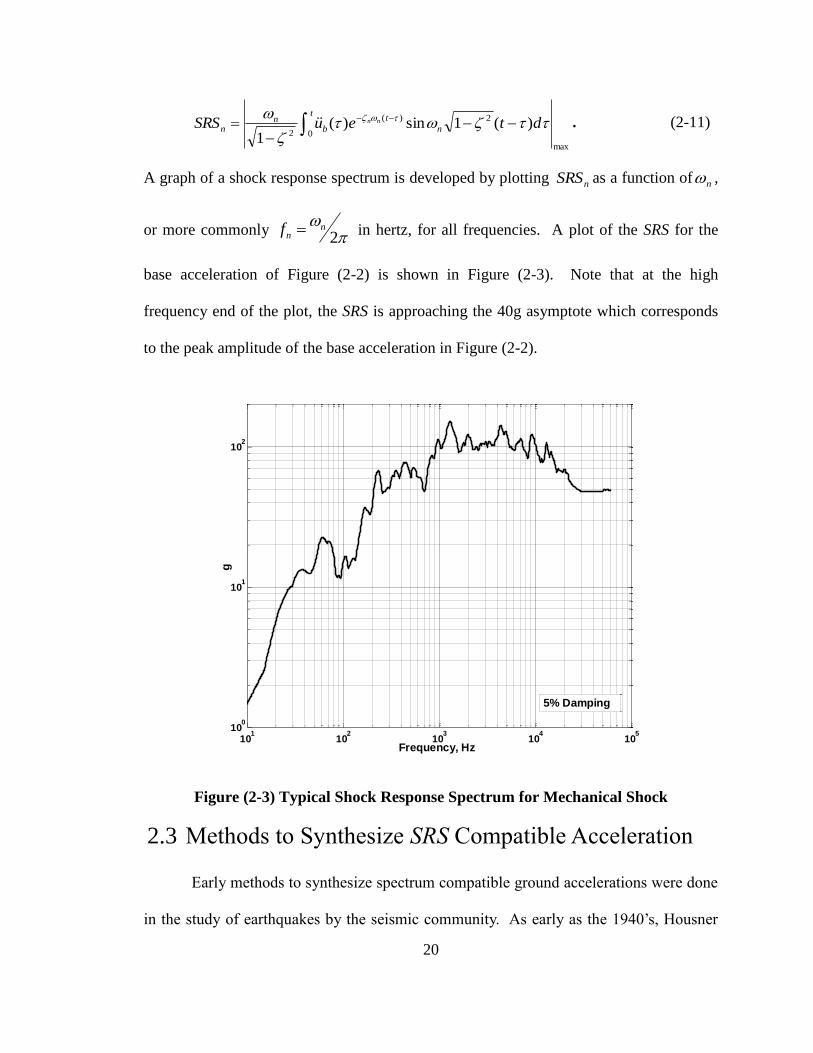
A graph of a shock response spectrum is developed by plotting nSRS as a function of n ,
or more commonly
2
nnf in hertz, for all frequencies. A plot of the SRS for the
base acceleration of Figure (2-2) is shown in Figure (2-3). Note that at the high
frequency end of the plot, the SRS is approaching the 40g asymptote which corresponds
to the peak amplitude of the base acceleration in Figure (2-2).
Figure (2-3) Typical Shock Response Spectrum for Mechanical Shock
2.3 Methods to Synthesize SRS Compatible Acceleration
Early methods to synthesize spectrum compatible ground accelerations were done
in the study of earthquakes by the seismic community. As early as the 1940’s, Housner
101
102
103
104
105
100
101
102
Frequency, Hz
g
5% Damping
21
(1947) modeled an earthquake as a random process with a series of pulses of different
magnitudes that occurred randomly in time. Subsequently, Housner (1955) used a
technique of modeling an earthquake as the sum of sine wave pulses occurring randomly
in time, with frequency and amplitude determined from a probability distribution.
Additional research to synthesize an SRS compatible acceleration time-history
was continued in the 1960’s by the seismic community. Civil engineers recognized the
need to model ground structures analytically to determine the survivability to withstand
strong earthquakes. Early methods to synthesize base accelerations compatible with a
prescribed design SRSD were approached by modifications of earthquake acceleration
records. These approaches were to use either stationary random processes (Housner &
Jennings, 1964) (Jennings, Housner, & Tsai, 1968) (Shinozuka, 1973) (Rizzo, Shaw, &
Jarecki, 1973) (Preumont, 1980) or non-stationary random processes (Iyengar & Iyengar,
1969) (Saragoni & Hart, 1974) (Iyengar & Rao, 1979) to guide the modification of
earthquakes acceleration data for the synthesis of an artificial earthquake. The approach
was to choose a starting set of coefficients for each frequency of SRSD and modify the set
iteratively to improve the agreement between the SRSS of the artificial earthquake and the
SRSD of the real earthquake (Preumont, 1984). Several starting procedures were explored
including.
Selection of an existing earthquake acceleration record which had an SRS that
was close to the target SRSD,
Selection of an initial set of coefficient by modification of the amplitude of
the Fourier transform of the existing earthquake and

22
Modification of the power spectral density (PSD) of the real earthquake for
the set of coefficients for each frequency.
During the 1970’s, procedures to synthesize SRSD compatible acceleration time-
histories emerged which did not rely on existing earthquake acceleration data records.
These methods employed the summation of sinusoids using a temporal envelope function
to control the rise and decay of the synthesized acceleration (Scanlan & Sachs, 1974)
(Gasparini & Vanmarcke, Jan 1976) (Levy & Wilkinson, 1976) (Kost, Tellkamp,
Gantayat, & Weber, 1978) (Ghosh, 1991) (Alexander J. E., 1995).
The introduction of neural networks in the 1990’s provided seismic engineers
other methods to synthesize spectrum compatible ground accelerations. One such
method was to train a two stage neural network from 30 earthquake ground acceleration
records (Ghaboussi & Lin, 1998). Another approach employed a five neural network
model to synthesize an SRSD compatible ground acceleration (Lee & Han, 2010). This
approach used basic earthquake information such as magnitude, epicenter distance, site
conditions and focal depth to train the neural networks. While neural network based
processes did result in a synthesized earthquake acceleration, limitations existed based on
departure of the earthquake of interest compared to those that trained the neural networks.
In general the match of the synthesized SRSS was not particularly accurate to the target
SRSD.
Soize (2010) published a unique method to synthesize aS to be compatible with
SRSD using the maximum entropy principal. This principle was used to construct the
23
probability distribution of a non-stationary stochastic process. The resulting aS waveform
appeared credible and the agreement between SRSS and SRSD was reasonable.
Brake (2011) published an interesting approach of combining different basis
functions to synthesize an SRS compatible base acceleration. These functions were
impulses, sines, damped sines and wavelets. With various combinations of these
functions and optimizing the coefficients of each with a genetic algorithm, Brake was
able to obtain a reasonable match of SRSS and SRSD. The resulting transient aS wave
form, however, was obviously a “manufactured” time-history with little temporal relation
to real test data.
Others in the seismic community continued to explore the synthesis of SRS
compatible ground acceleration time-histories using the stationary and non-stationary
features of earthquakes to include the power spectral density function (Gupta & Trifunac,
1998) (Zhang, Chen, & Li, 2007).
Presently for mechanical shock, the most common techniques to synthesize an
SRS compatible acceleration aS are:
classical pulse (e.g., half-sine, terminal peak saw-tooth, trapezoid),
damped sinusoids,
wavelets and
enveloped sinusoids.
MIL-STD-810G, Method 516 (Department of Defense, 2008) specifies that if test data
are not available, the use of damped or amplitude modulated sinusoids is permissible
provided that the SRSS exceeds a prescribed SRSD over a frequency range of 5-2000 Hz.
24
The use of a classical pulse (either terminal peak saw-tooth or trapezoid), while the least
desirable approach, is permitted if no test data are available. The UK MOD (Ministry of
Defense, 2006) also imposes requirements and tolerances on pulses (half sine, terminal
peak saw-tooth, and trapezoidal) and damped sinusoids in terms of peak amplitude and
number of shocks pulses.
Beyond classical shock pulses to synthesize an SRSD compatible aS, some variant
of the summation of sinusoids is the most frequently used method for mechanical shock.
One method, especially relevant for control an electro-dynamics shaker test machine, is
wavelets (Irvine, 2015). Multiple discrete wavelets, when summed, will result in a
synthesized aS wave form. A discrete wavelet has a sinusoidal motion with a finite and
specific number of half sine oscillations with unique parameters for frequency, amplitude
and time delay. Iterations for the parameters of each wavelet yield a synthesized aS with
a resulting SRSS that matches SRSD within acceptable tolerances. The equation for an
individual wavelet, Wn(t), is given by,
(2-12)
(2-13)
(2-14)
(2-15)
where,
nN
n
nS
n
ndnn
n
ndndndnndn
n
nnn
dnn
tWta
NtttW
Nttttttt
NAtW
tttW
1
0
sinsin
0
25
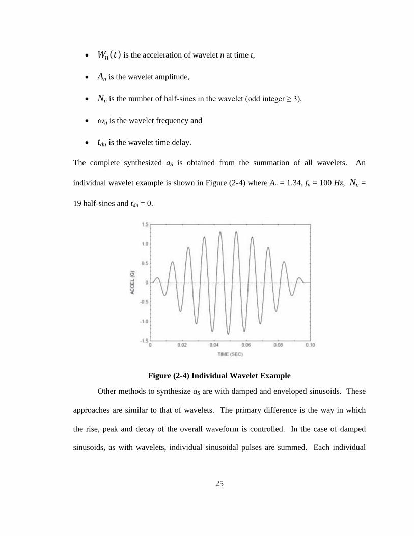
𝑊𝑛(𝑡) is the acceleration of wavelet n at time t,
An is the wavelet amplitude,
Nn is the number of half-sines in the wavelet (odd integer ≥ 3),
ωn is the wavelet frequency and
tdn is the wavelet time delay.
The complete synthesized aS is obtained from the summation of all wavelets. An
individual wavelet example is shown in Figure (2-4) where An = 1.34, fn = 100 Hz, Nn =
19 half-sines and tdn = 0.
Figure (2-4) Individual Wavelet Example
Other methods to synthesize aS are with damped and enveloped sinusoids. These
approaches are similar to that of wavelets. The primary difference is the way in which
the rise, peak and decay of the overall waveform is controlled. In the case of damped
sinusoids, as with wavelets, individual sinusoidal pulses are summed. Each individual

26
damped sine pulse has a unique time delay tdn, damping ζn, amplitude An, and frequency
ωn defined by,
(2-16)
(2-17)
(2-18)
An example of an individual damped sine pulse is shown in Figure (2-5) where An =
1.34g, fn = 100 Hz, ζ=0.05 and tdn = .01 seconds.
Figure (2-5) Individual Damped Sine Example
The enveloped sinusoids with random phase angles approach is similar to damped
sinusoids. The equation for enveloped sinusoids is given by,
, (2-19)
where An are the amplitude coefficients, ωn are the frequencies of the sinusoids and φn are
random phase angles for each frequency n. The rise, plateau and decay of aS is controlled
by an envelope function E(t) rather than damping. Since E(t) can be sized to any
0 0.02 0.04 0.06 0.08 0.1-1.5
-1
-0.5
0
0.5
1
1.5
TIME (SEC)
AC
CE
L (
G)
.
sin
,,0
1
N
n
nS
dndnn
tt
nn
dnn
tWta
andtttteAtW
tttW
dnnn
N
n
nnnS tAtEta1
sin
27
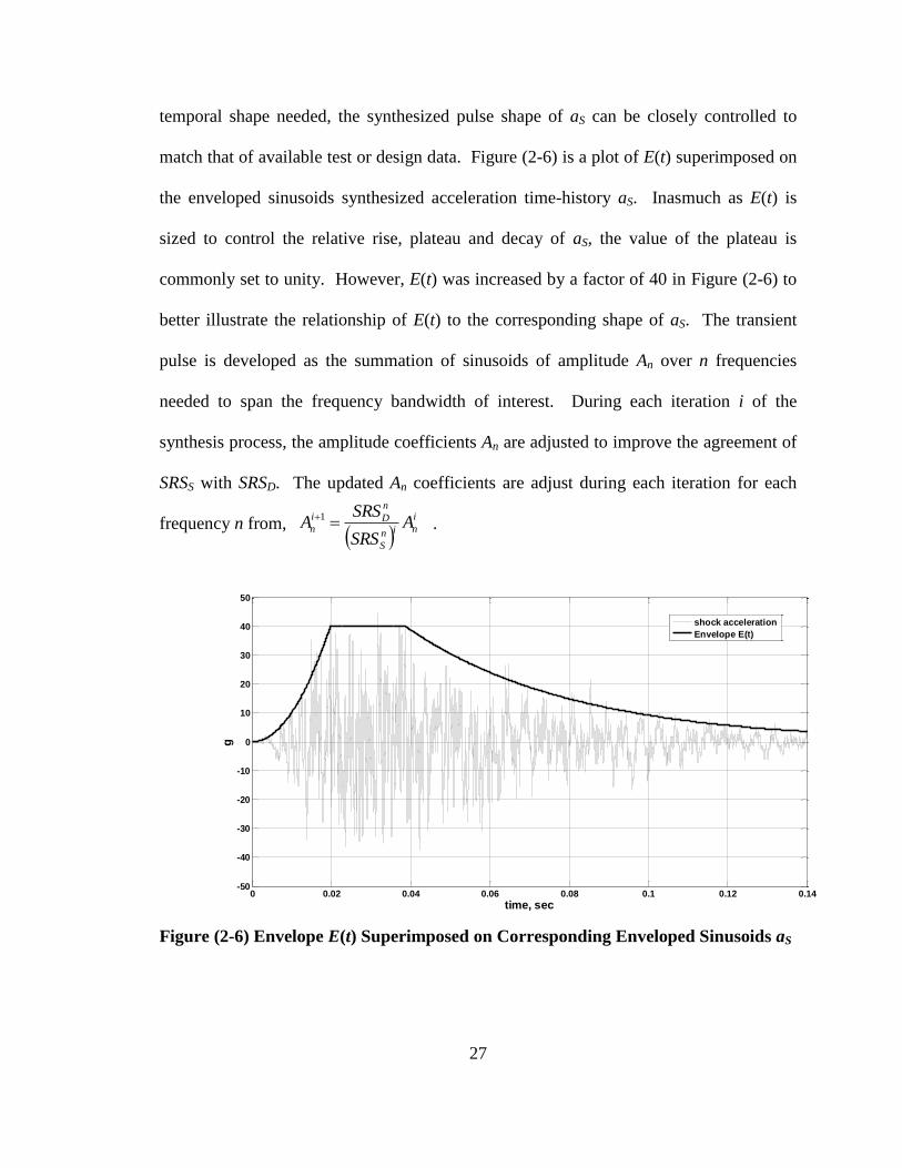
temporal shape needed, the synthesized pulse shape of aS can be closely controlled to
match that of available test or design data. Figure (2-6) is a plot of E(t) superimposed on
the enveloped sinusoids synthesized acceleration time-history aS. Inasmuch as E(t) is
sized to control the relative rise, plateau and decay of aS, the value of the plateau is
commonly set to unity. However, E(t) was increased by a factor of 40 in Figure (2-6) to
better illustrate the relationship of E(t) to the corresponding shape of aS. The transient
pulse is developed as the summation of sinusoids of amplitude An over n frequencies
needed to span the frequency bandwidth of interest. During each iteration i of the
synthesis process, the amplitude coefficients An are adjusted to improve the agreement of
SRSS with SRSD. The updated An coefficients are adjust during each iteration for each
frequency n from, .
Figure (2-6) Envelope E(t) Superimposed on Corresponding Enveloped Sinusoids aS
0 0.02 0.04 0.06 0.08 0.1 0.12 0.14-50
-40
-30
-20
-10
0
10
20
30
40
50
time, sec
g
shock acceleration
Envelope E(t)
i
nin
S
n
Di
n ASRS
SRSA 1
28
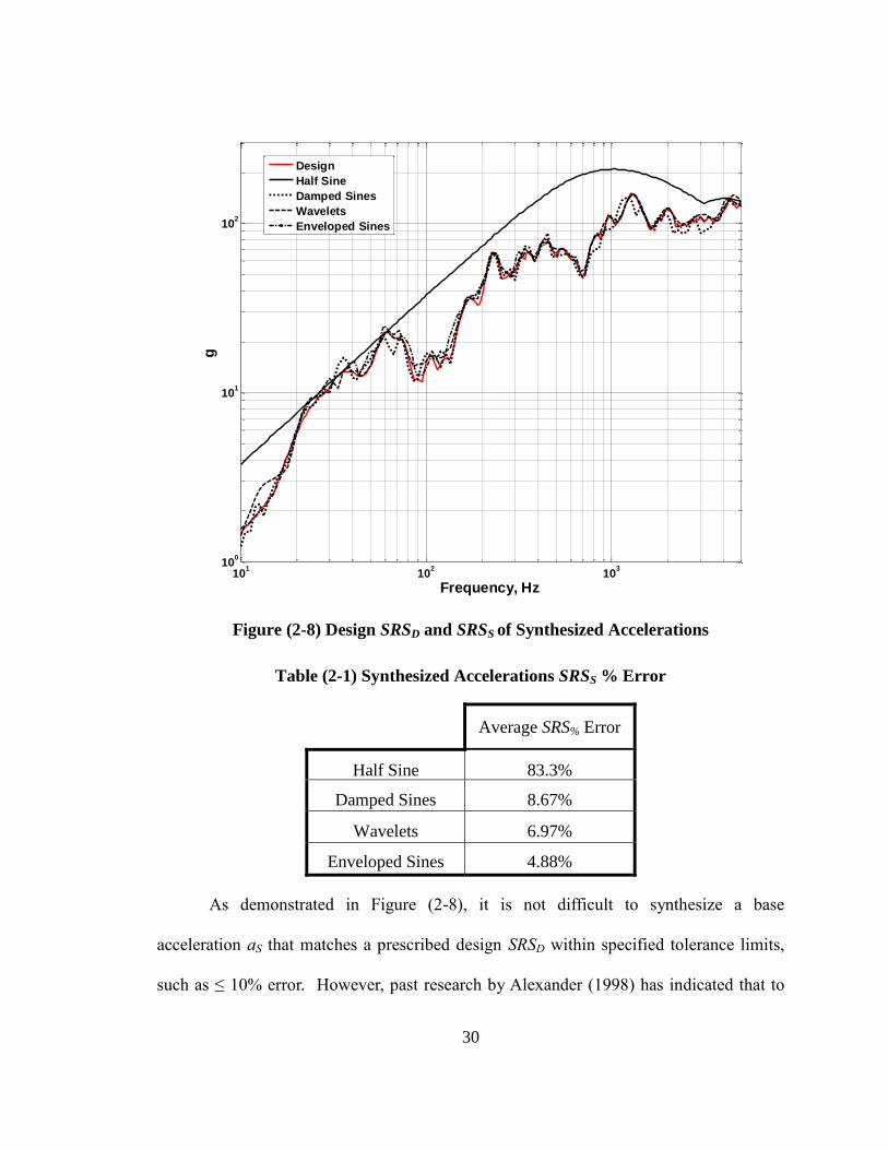
Figure (2-7) is a plot of the design acceleration aD and four accelerations (half
sine, damped sines, wavelets and enveloped sines) synthesized to match SRSD. No
attempt was made to match the energy input spectrum or duration of aD, EIS and TE,
respectively. The time scale of the half sine pulse was expanded by a factor of ten
relative to the others in Figure (2-7), to better show the shape of the synthesized
waveform. The SRSS of the synthesized accelerations, with the exception of the half sine,
matched SRSD with good agreement. Figure (2-8) shows SRSD and SRSS for the four
synthesized aS. Table (2-1) is the percentage errors for the SRSS of the synthesized
accelerations relative to SRSD. The percentage error for each is the percent difference
between SRSS and SRSD averaged over all the frequencies. The error was least for
enveloped sines at 4.88% .

29
Figure (2-7) Design aD and Synthesized Accelerations
0 0.04 0.08 0.12 0.14-50
-25
0
25
50
time, secg
Design aD
0 0.004 0.008 0.012 0.0140
50
100
150
aS Half Sine time, sec
g
0 0.04 0.08 0.12 0.14-50
-25
0
25
50
time, sec
g
aS Damped Sines
0 0.04 0.08 0.12 0.14-50
-25
0
25
50
g
aS Wavelets
time, sec
0 0.04 0.08 0.12 0.14-50
-25
0
25
50
aS Enveloped Sines time, sec
g
30
Figure (2-8) Design SRSD and SRSS of Synthesized Accelerations
Table (2-1) Synthesized Accelerations SRSS % Error
Average SRS% Error
Half Sine 83.3%
Damped Sines 8.67%
Wavelets 6.97%
Enveloped Sines 4.88%
As demonstrated in Figure (2-8), it is not difficult to synthesize a base
acceleration aS that matches a prescribed design SRSD within specified tolerance limits,
such as ≤ 10% error. However, past research by Alexander (1998) has indicated that to
101
102
103
100
101
102
Frequency, Hz
g
Design
Half Sine
Damped Sines
Wavelets
Enveloped Sines
31
obtain an accurate response from a structural dynamic model, matching only the SRSD is
not sufficient. While a specific base acceleration transient will result in a unique shock
response spectrum, the inverse is not true. There are theoretically an infinite number of
base accelerations that will yield the same SRS. The phasing of the modes of a structural
dynamic model relative to the timing of the synthesized acceleration peaks can
significantly affect peak MDOF response magnitudes. The goal of the research herein is
to determine a process, with additional guidelines beyond common practices, that will
yield not only a spectrum compatible synthesized base acceleration, but also will yield
improved results when applied to linear and nonlinear physical system models, especially
for energy input. To improve the accuracy of a physical system model response to as,
additional constraints are explored for the acceleration synthesis process. One such
constraint is temporal (time) duration of the synthesized transient acceleration pulse. If
test data have been acquired, temporal information can be determined from the data set to
guide the synthesis of aS. For example MIL-STD-810G, Method 516 (Department of
Defense, 2008) imposes temporal durations termed TE and Te on the synthesized
acceleration as. Additionally, an average or maximum EIS can be determined from the
test data set.
2.4 Evolution of Energy Methods for Shock and Vibration
Research of energy methods for transient shock response modeling provides
another constraint to be applied in the synthesis of aS. This involves compatibility with
not only the SRSD, but also with the EISD. Synthesis of aS to be compatible with SRSD,
EISD and temporal duration TED offer additional constraints to be considered for the
objective of improving MDOF system response accuracy.

32
The seismic community did much of the early research to examine the utility of
base acceleration energy input. The use of energy to characterize base excited structural
dynamic response dates back to Hudson (1956) and Housner (1959). Hudson
documented the maximum energy per unit mass for a SDOF oscillator is given by
relationship to the velocity shock response spectrum,
(2-20)
Hudson further developed a relationship between the velocity spectrum and the total
energy from a series of pulses similar to that of earthquake excitation. Housner derived
a relationship for the average energy in a MDOF structure based on the superposition of
the total modal energies for each of the normal modes of the structure. The average
energy in the structure for a transient shock is given as a function of the total mass of the
structure and the average of the squared velocity spectral value of all N normal modes of
the structure,
. (2-21)
Other authors who have documented the relationship between energy and the square of
the velocity spectrum include (Zahrah & Hall, 1984) (Uang & Berto, 1990) (Edwards,
2007).
Shock motion can be characterized by energy delivered to a structure. It is
possible to determine energy input from a base acceleration-time history, and from the
conservation of energy, the input energy will balance the energy from system response.
The EIS is similar to an SRS inasmuch as it is a frequency based measure of the response
of a series of SDOF oscillators subjected to a common base acceleration. However, in
the case of an EIS, the measure is peak energy input per unit mass to the SDOF oscillator
.2
1max 2
velSRSmassunit
energy
avevelave n
SRSMEnergy 2
2
1
33
from the base acceleration, instead of peak mass acceleration response as in the case of
the SRS. As with the SRS, peak energy input is determined for a series of SDOF
oscillators covering the frequency bandwidth of interest. Derivation of the EIS is in
developed Section 2.5.
As was the case for the SRS, much of the ground work to study base excitation of
a structure in terms of energy, in general, and the development of the EIS, in particular,
was done by the seismic community from the mid-1980’s to the present. Zahrah and Hall
(1984) investigated the response of simple SDOF structures from strong earthquake
excitations. Eight earthquakes records of magnitudes 4.7 to 7.7 were selected for
representative strong ground input motions. The objective of the study was to better
quantify factors that influence structural deformation and damage. The approach of the
study was to compare the input energy to the dissipated energy by inelastic deformations
and damping, to establish an improved damage criteria than peak ground acceleration or
the shock response spectrum. The conclusion of the study was that a better damage
potential might be defined in terms of the energy input to the structure.
Two formulation of the energy input equation are possible, based on absolute and
relative coordinates for the SDOF equation of motion. The relative energy equation is
given by (2-28). The absolute energy equation is based on derivation of the energy terms
from the SDOF equation of motion prior to making the substitution for the relative
coordinate (z=u-ub). The absolute formulation leads to the energy input term (EIabs
=∫ 𝑚�̈� 𝑑𝑢𝑏). Uang and Bertero (1990) used the absolute energy formulation to compare
the results of the input energy per unit mass from the SDOF EIS with that of a linear
multi-story building. The result was the energy input of the SDOF model, on a per unit
34
mass basis, provided a very good estimate of the input energy of the multi-story building
for the dominant frequency.
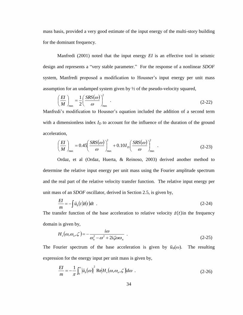
Manfredi (2001) noted that the input energy EI is an effective tool in seismic
design and represents a “very stable parameter.” For the response of a nonlinear SDOF
system, Manfredi proposed a modification to Housner’s input energy per unit mass
assumption for an undamped system given by ½ of the pseudo-velocity squared,
(2-22)
Manfredi’s modification to Housner’s equation included the addition of a second term
with a dimensionless index ID to account for the influence of the duration of the ground
acceleration,
(2-23)
Ordaz, et al (Ordaz, Huerta, & Reinoso, 2003) derived another method to
determine the relative input energy per unit mass using the Fourier amplitude spectrum
and the real part of the relative velocity transfer function. The relative input energy per
unit mass of an SDOF oscillator, derived in Section 2.5, is given by,
(2-24)
The transfer function of the base acceleration to relative velocity �̇�(𝑡)in the frequency
domain is given by,
(2-25)
The Fourier spectrum of the base acceleration is given by �̈�b(ω). The resulting
expression for the energy input per unit mass is given by,
(2-26)
.
2
12
maxmax
SRS
M
EI
.10.045.0
2
max
2
maxmax
SRSI
SRS
M
EID
. dttztum
EIb
.2
,,22
nn
nvi
iH
.,,Re1 2
0
dHu
m
EInvb
35
Initial research and development for the use of energy methods was done almost
exclusively by the seismic community to characterize shock damage from earthquakes.
More recently other authors have published research in the application of energy methods
to characterize mechanical shock as an alternative to the SRS. Authors who have
considered energy methods for damage potential to mechanical systems include Gaberson
(1995), Edwards (2007) (2009) , Iwasa and Shi (2008), and Alexander (2011).
Gaberson (1995) was a passionate advocate for the velocity shock response
spectrum, SRSvel, as a measure of damage potential. One of Gaberson’s arguments for the
use of the SRSvel was the relationship to energy (½ mSRS2
vel), first noted by Hudson
(1956).
Iwasa and Shi (2008) advocated the maximum total energy spectrum as the best
measure of damage potential in the context of pyroshock, and noted that past studies
indicated that maximum acceleration does not consistently represent the most accurate
measure of damage potential. Their conclusion was that the maximum energy per unit
mass of an SDOF system is a suitable indicator of pyroshock damage potential. This was
confirmed by two mechanical tests, one from impact and one from electro-dynamic
shaker input.
Based on a numerical simulation, Edwards (2007) demonstrated that the
maximum energy input per unit mass input to a MDOF structure can be estimated by the
energy input per unit mass of an SDOF system (i.e., the EIS) with the same frequency of
the lowest (dominant) frequency of the MDOF structure. Uang and Berto (1990)
demonstrated a similar finding. Edward’s simulation consisted of five nonlinear 4DOF
36
systems with the pre-yield fundamental frequencies of 10 Hz, 285 Hz, 1716 Hz, 7,357 Hz
and 19,739 Hz. In all five cases, the energy input per unit mass of the 4DOF structure
matched the EIS at those same frequencies with good agreement.
Alexander (2011) published a study comparing the EIS from two base
accelerations with the maximum energy per unit mass from the response of a 6DOF
ABAQUS (Dassault Systemes Simulia Corp, 2008) model, for both linear and nonlinear
versions of model. The maximum energy per unit mass comparison from the model had
good agreement with the EIS for the linear model. The same comparison for the
nonlinear version of the model, while not unreasonable, had mixed results depending on
the frequency.
Honeywell (Hartwig, 2013) was able to successfully use the EIS to quantify the
total damage potential from packaging, handling and vibration from two different
Honeywell operations. The EIS was developed for each of the two sites from data
collected for each packaging configuration and each mode of transportation. Hartwig
noted that the benefit of the EIS was that it accounts for the duration of the events and
repeated exposures, where the power spectral density (PSD) does not. The same issue
exists with the SRS.
2.5 Derivation of the Energy Input Equations
As with the SRS, it is possible to determine an Energy Input Spectrum (EIS), from
a base acceleration from the peak energy inputs to a series of SDOF oscillators of
different frequencies. A series of linear damped SDOF oscillators mounted to a common
base, Figure (2-1), is also applicable for development of an EIS. Equation (2-3) is the
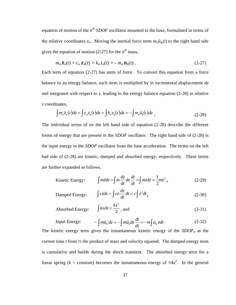
37
equation of motion of the nth
SDOF oscillator mounted to the base, formulated in terms of
the relative coordinates zn. Moving the inertial force term mn�̈�𝑏(t) to the right hand side
gives the equation of motion (2-27) for the nth
mass,
mn �̈�n(t) + cn �̇�n(t) + kn zn(t) = - mn �̈�b(t) . (2-27)
Each term of equation (2-27) has units of force. To convert this equation from a force
balance to an energy balance, each term is multiplied by in incremental displacement dz
and integrated with respect to z, leading to the energy balance equation (2-28) in relative
z coordinates,
. (2-28)
The individual terms of on the left hand side of equation (2-28) describe the different
forms of energy that are present in the SDOF oscillator. The right hand side of (2-28) is
the input energy to the SDOF oscillator from the base acceleration. The terms on the left
had side of (2-28) are kinetic, damped and absorbed energy, respectively. These terms
are further expanded as follows.
Kinetic Energy: , (2-29)
Damped Energy: , (2-30)
Absorbed Energy: , and (2-31)
Input Energy: . (2-32)
The kinetic energy term gives the instantaneous kinetic energy of the SDOFn at the
current time t from ½ the product of mass and velocity squared. The damped energy term
is cumulative and builds during the shock transient. The absorbed energy term for a
linear spring (k = constant) becomes the instantaneous energy of ½kz2. In the general
dztumdztzkdztzcdztzm bnnnnnnn
2
2
1zmzdzm
dt
dtdz
dt
zdmdzzm
2
2kzkzdz
dtzumdt
dtdzumdzum bbb
dtzcdtdt
dzzcdzzc 2
38
case where there is inelastic behavior of the spring (e.g., elasto-plastic) the absorbed
energy would be cumulative during the transient due to plastic strain. Equation (2-32)
gives the input energy to the SDOFn from the base acceleration and relative velocity. The
input energy is cumulative for the duration of the shock transient. For any instance in
time, the input energy is equal to the sum of the response energy terms on the left hand
side of equation (2-28). An updated energy equation for the motion of a linear SDOFn
oscillator is given by equation (2-33),
. (2-33)
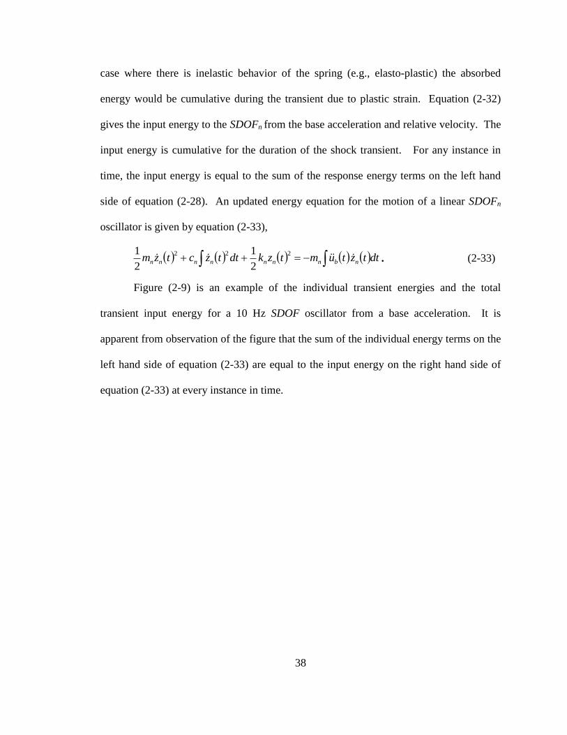
Figure (2-9) is an example of the individual transient energies and the total
transient input energy for a 10 Hz SDOF oscillator from a base acceleration. It is
apparent from observation of the figure that the sum of the individual energy terms on the
left hand side of equation (2-33) are equal to the input energy on the right hand side of
equation (2-33) at every instance in time.
dttztumtzkdttzctzm nbnnnnnnn
222
2
1
2
1
39
Figure (2-9) Transient Energy Input for 10 Hz SDOF
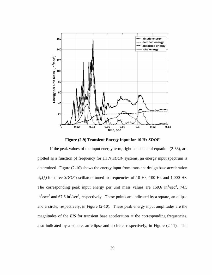
If the peak values of the input energy term, right hand side of equation (2-33), are
plotted as a function of frequency for all N SDOF systems, an energy input spectrum is
determined. Figure (2-10) shows the energy input from transient design base acceleration
𝑢�̈�(𝑡) for three SDOF oscillators tuned to frequencies of 10 Hz, 100 Hz and 1,000 Hz.
The corresponding peak input energy per unit mass values are 159.6 in2/sec
2, 74.5
in2/sec
2 and 67.6 in
2/sec
2, respectively. These points are indicated by a square, an ellipse
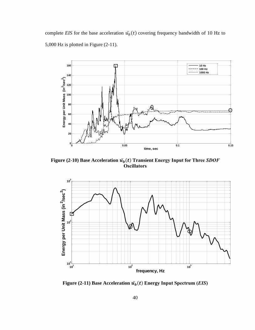
and a circle, respectively, in Figure (2-10). These peak energy input amplitudes are the
magnitudes of the EIS for transient base acceleration at the corresponding frequencies,
also indicated by a square, an ellipse and a circle, respectively, in Figure (2-11). The
0 0.02 0.04 0.06 0.08 0.1 0.12 0.140
20
40
60
80
100
120
140
160
time, sec
En
erg
y p
er
Un
it M
ass
(i
n2/s
ec
2)
kinetic energy
damped energy
absorbed energy
total energy
40
complete EIS for the base acceleration 𝑢�̈�(𝑡) covering frequency bandwidth of 10 Hz to
5,000 Hz is plotted in Figure (2-11).
Figure (2-10) Base Acceleration 𝒖�̈�(𝒕) Transient Energy Input for Three SDOF
Oscillators
Figure (2-11) Base Acceleration 𝒖�̈�(𝒕) Energy Input Spectrum (EIS)
0 0.05 0.1 0.150
20
40
60
80
100
120
140
160
time, sec
En
erg
y p
er
Un
it M
ass
(i
n2/s
ec
2)
10 Hz
100 Hz
1000 Hz
101
102
103
101
102
103
frequency, Hz
En
erg
y p
er
Un
it M
ass (
in2/s
ec
2)
41
Derivation of an the energy equation for a MDOF structure is similar to that of a
SDOF oscillator, and modifications to the MDOF matrix equation of motion are also
similar to that of the SDOF scalar equation of motion. For a linear MDOF system in
relative coordinates, the matrix equation of motion is given by equation (2-34),
. (2-34)
To convert equation (2-34) to from a force balance to an energy balance, we again
multiply each term by {dz} T
and integrate with respect to z, leading to the MDOF energy
equation (2-35),
. (2-35)
Noting that {dz} can be rewritten as , this substitution in (2-35) for all terms,
except the absorbed energy term results in,
(2-36)
If similar transformations are executed for (2-36) as was done for the SDOF energy
terms, equation (2-29) through equation (2-32) , the same energy terms occur for the
MDOF system, given by,
Kinetic Energy: , (2-37)
Damped Energy: (2-38)
Absorbed Energy: and (2-39)
Input Energy: (2-40)
For the 3DOF system models described in Chapters 3 and 4, the input energy was
computed from equation (2-40). The time integration was performed using the central
dtdt
dz
.1 dtuMzzKdzdtzCzdtzMz b
TTTT
zMzT
2
1
,dtzCzT
zKzT
2
1
.1 dtuMz b
T
buMzKzCzM 1
b
TTTTuMdzzKdzzCdzzMdz 1
42
difference numerical integration time stepping routine, where the dynamic analysis is
executed by stepping through the transient with equal Δt time increments. The
integration procedure evaluates the incremental ΔEkn input energy for current time step
increment k, and adds ΔEkn to the cumulative sum of all prior time steps, En
k-1. The
3DOF energy input time stepping procedure is,
(2-41)
(2-42)
(2-43)
2.6 Temporal Information from a Shock Acceleration
In addition to the SRS and EIS, if temporal information is available from shock
test data it offers additional information for the synthesis of aS. Two characteristics of a
typical shock acceleration time-history are the overall envelope shape and a strong shock
duration.
The envelope E(t) is the relative temporal shape of the overall rise, plateau and
decay of the shock acceleration time-history. Since E(t) is a relative shape of the shock
acceleration, the plateau is typically set to 1.0. For a family of test data, E(t) can be
determined based on a best fit of the data. Although various shapes are possible,
mechanical shock acceleration is frequently characterized by a rapid exponential rise, a
relative short plateau region, followed by a more gradual exponential decay. E(t) has the
same characteristics.
.
1
1
1
00
00
00
,
332211
1
3
2
1
321
1
1
tuzmzmzmEE
andtu
m
m
m
zzzEE
EEE
k
b
k
n
k
n
k
b
kk
n
k
n
k
n
k
n
k
n
43
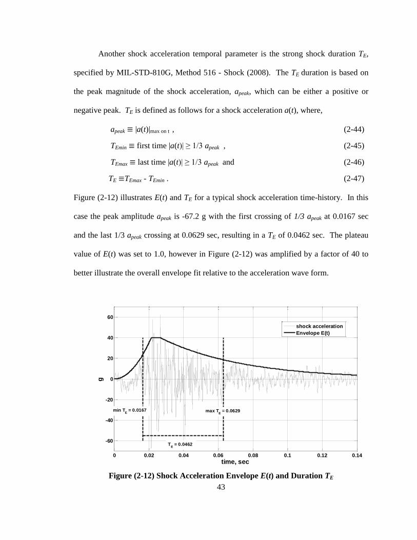
Another shock acceleration temporal parameter is the strong shock duration TE,
specified by MIL-STD-810G, Method 516 - Shock (2008). The TE duration is based on
the peak magnitude of the shock acceleration, apeak, which can be either a positive or
negative peak. TE is defined as follows for a shock acceleration a(t), where,
apeak ≡ |a(t)|max on t , (2-44)
TEmin ≡ first time |a(t)| ≥ 1/3 apeak , (2-45)
TEmax ≡ last time |a(t)| ≥ 1/3 apeak and (2-46)
TE ≡TEmax - TEmin . (2-47)
Figure (2-12) illustrates E(t) and TE for a typical shock acceleration time-history. In this
case the peak amplitude apeak is -67.2 g with the first crossing of 1/3 apeak at 0.0167 sec
and the last 1/3 apeak crossing at 0.0629 sec, resulting in a TE of 0.0462 sec. The plateau
value of E(t) was set to 1.0, however in Figure (2-12) was amplified by a factor of 40 to
better illustrate the overall envelope fit relative to the acceleration wave form.
Figure (2-12) Shock Acceleration Envelope E(t) and Duration TE
0 0.02 0.04 0.06 0.08 0.1 0.12 0.14
-60
-40
-20
0
20
40
60
time, sec
g
shock acceleration
Envelope E(t)
TE = 0.0462
max TE = 0.0629min T
E = 0.0167

44
2.7 Define Baseline aD, SRSD, EISD and TED for Present
Study
Previously in this document, references have been made to a design acceleration
aD and the corresponding design shock response spectrum SRSD. For the present study, a
design acceleration time-history signal aD was chosen from a typical set of mechanical
shock test data. The aD chosen had an envelope shape and peak amplitude representative
of a mechanical shock pulse. The corresponding design shock response spectrum SRSD,
energy input spectrum EISD, temporal duration TED and envelope E(t) were determined
from aD. Figure (2-13) is a plot of aD with the corresponding TED and E(t) indicated on
the plot. The peak value of the envelope E(t) was 1.0, but was expanded by a factor of 47
in the plot to illustrate the fit with aD. Figure (2-14) is a plot of SRSD and EISD.
For the present study, these design quantities were needed as a basis of
comparison to evaluate the accuracy of synthesized accelerations aS. These evaluations
are the degree to which,
SRSS, EISS and TES match the corresponding quantities from aD, and
The accuracy of response of MDOF models from aS compared to the
corresponding response from aD.
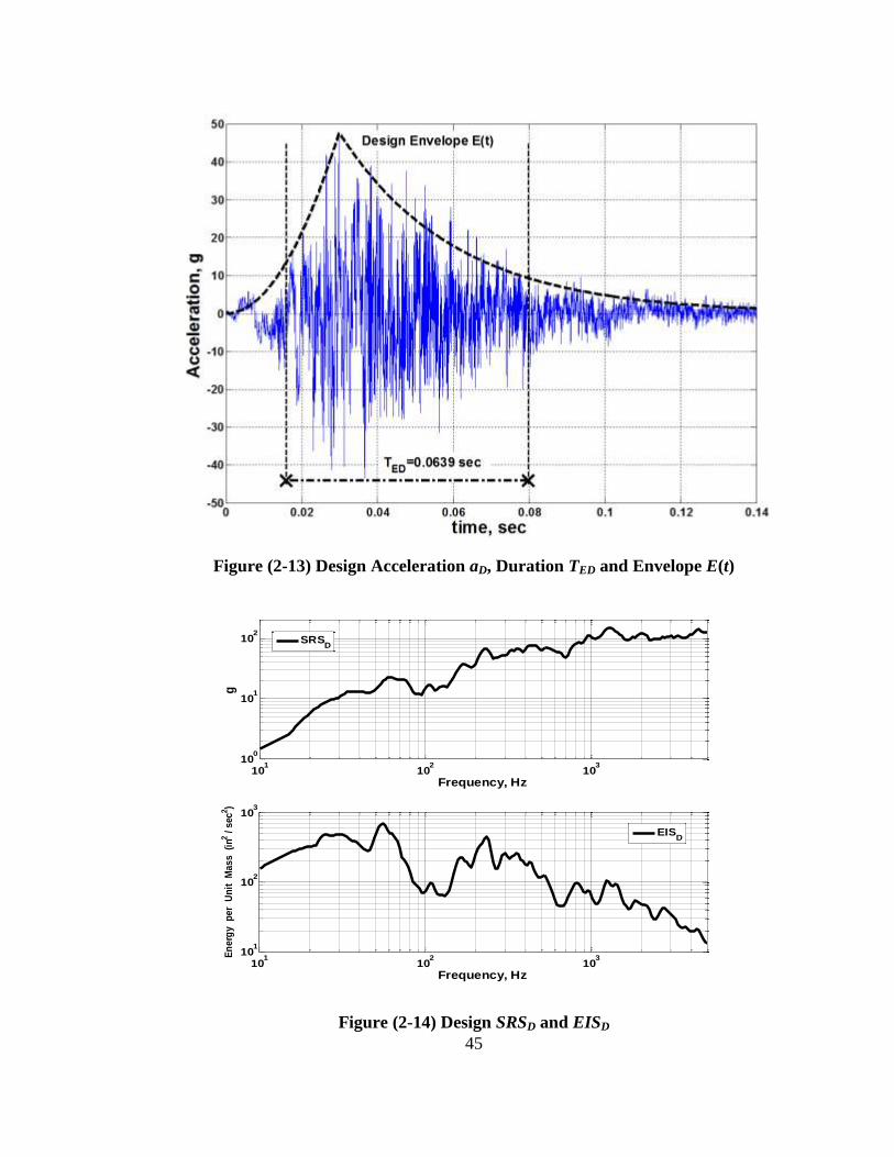
45
Figure (2-13) Design Acceleration aD, Duration TED and Envelope E(t)
Figure (2-14) Design SRSD and EISD
101
102
103
100
101
102
Frequency, Hz
g
101
102
103
101
102
103
Frequency, Hz
En
erg
y p
er
Un
it
Ma
ss
(in
2 /
sec
2)
SRSD
EISD
46
3 New Approach to Synthesize SRS
Compatible Acceleration
3.1 Overview
A new approach is described for the synthesis of an SRS compatible base
acceleration beyond what has been proposed and implemented in the past. This includes
the introduction of additional constraints beyond only SRSD compatibility of the
synthesized acceleration, aS. These additional constraints for aS are the design energy
input spectrum (EISD) and a design temporal duration TED. Given the objective to match
multiple constraints, a comprehensive synthesis procedure was required. Two essential
differences between how others have determined aS and the proposed approach are
specifically,
aS compatibility with EISD and TED, in addition to SRSD, and
Quality of aS evaluated based on the accuracy of MDOF model response.
3.2 Traditional Synthesize Methods of SRSD Compatible
Base Acceleration
As described in Chapter 2, past authors have documented numerous methods to
synthesize an SRSD compatible base acceleration. Common synthesis methods include
standard wave forms, typically comprised of a classical pulse or some variant of a
summation of sinusoids. These methods include:
Classical acceleration pulse (half sine, trapezoid, triangle, others),
Damped sinusoids,
Wavelets and
47
Enveloped sinusoids with random phase angles.
Less commonly used methods include trained neural networks, inverse Fourier
transforms, and maximum entropy.
Regardless of the method, authors have primarily addressed a single objective to
synthesize a base acceleration, aS, that returns a shock response spectrum, SRSS, which
matches the design shock response spectrum, SRSD, within prescribed limits. For
example, MIL-STD-810G, Method 516.6 (2008) prescribes a tolerance envelope of +3.0
dB/-1.5 dB around SRSD which SRSS is to meet. This single objective obviates the
motivation to make use of other significant information including input energy and
temporal data of the input shock acceleration transient. Specifically:
Input energy per unit mass of aS, characterized by an energy input spectrum
EISS. The EIS of a general base acceleration �̈�𝑏(t) is given by the right hand
side of equation (2-33) and as plotted in Figure (2-11).
Temporal duration TE for the shock acceleration time duration. TE is used as a
constraint on the duration of the strong shock region of the synthesized
acceleration aS. TE is based on the peak amplitude of a shock acceleration
time-history as defined in Chapter 2, equations (2-44) through (2-47).
Transient shock shape envelope E(t).
3.3 Synthesis of Base Acceleration aS
The objective of the synthesis procedure is to determine aS which is compatible
with the corresponding design acceleration quantities of SRSD, EISD, TED and E(t). To
achieve this, the differences between synthesis based quantities SRSS, EISS, and TES and
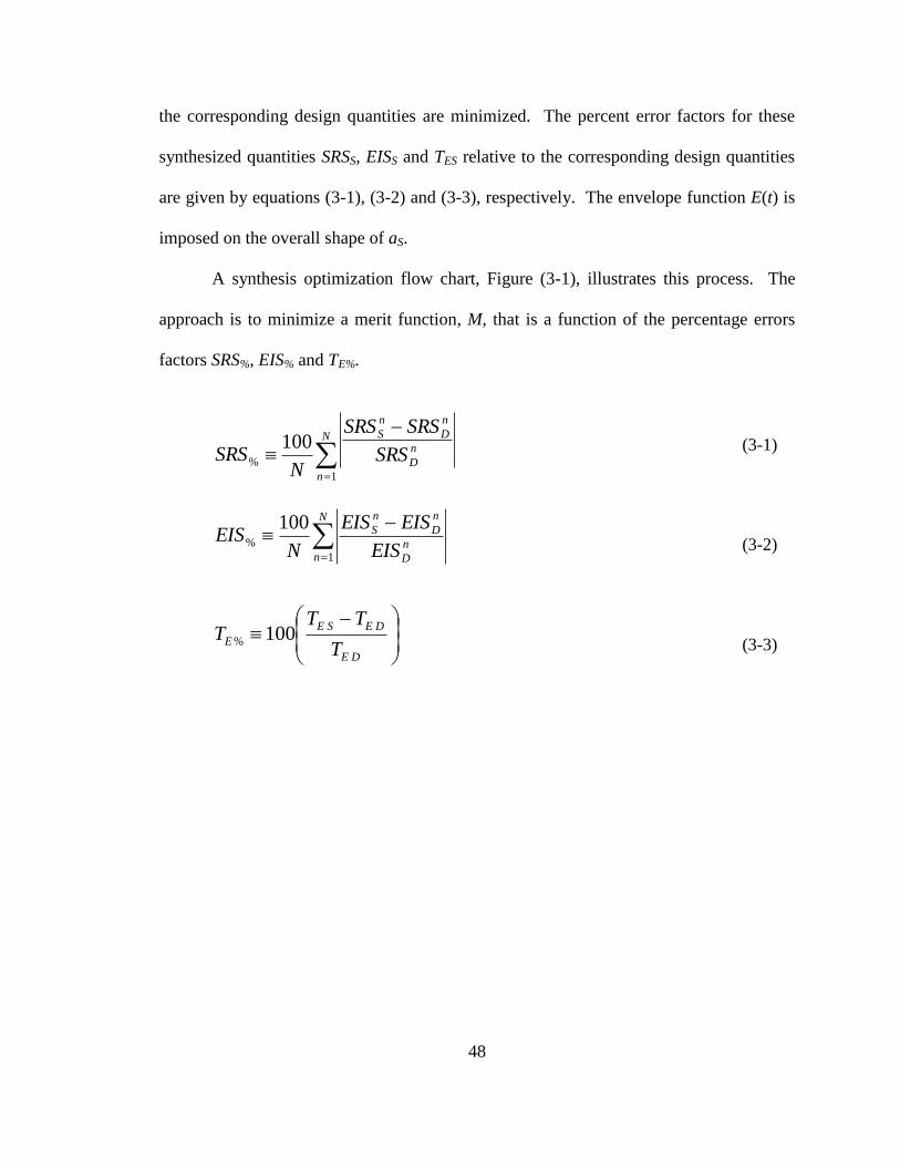
48
the corresponding design quantities are minimized. The percent error factors for these
synthesized quantities SRSS, EISS and TES relative to the corresponding design quantities
are given by equations (3-1), (3-2) and (3-3), respectively. The envelope function E(t) is
imposed on the overall shape of aS.
A synthesis optimization flow chart, Figure (3-1), illustrates this process. The
approach is to minimize a merit function, M, that is a function of the percentage errors
factors SRS%, EIS% and TE%.
(3-1)
(3-2)
(3-3)
DE
DESE
E
N
nn
D
n
D
n
S
N
n
n
D
n
D
n
S
T
TTT
EIS
EISEIS
NEIS
SRS
SRSSRS
NSRS
100
100
100
%
1
%
1
%
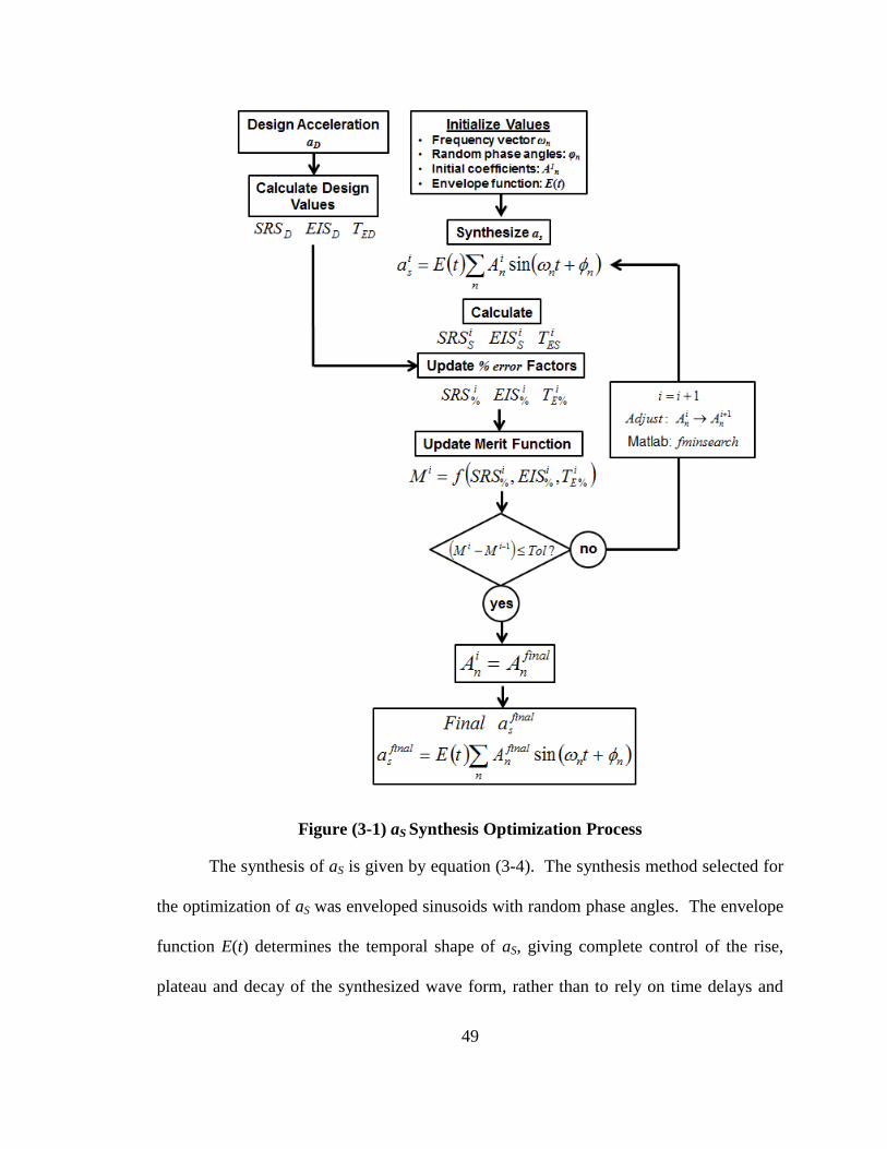
49
Figure (3-1) aS Synthesis Optimization Process
The synthesis of aS is given by equation (3-4). The synthesis method selected for
the optimization of aS was enveloped sinusoids with random phase angles. The envelope
function E(t) determines the temporal shape of aS, giving complete control of the rise,
plateau and decay of the synthesized wave form, rather than to rely on time delays and
50
damping of individual sinusoids. Based on examination of mechanical shock acceleration
data, a typical shock pulse has a rapid rise, a brief (if any) plateau, and a gradual decay.
The correct choice of E(t) assures this shape for aS. It has proven to be effective in
matching the temporal profile of aD, or the combined envelope in the case of a family of
field data.
(3-4)
The synthesis procedure is iterative as shown in Figure (3-1). The summation in equation
(3-4) is over the index n corresponding to all SRSD N ωn frequencies. The amplitude
coefficients An for each sinusoid are independently updated in each iteration to
minimization the merit function M. To start the procedure, the following initial quantities
are set.
Temporal envelope function E(t).
Frequency vector ωn to span the frequency bandwidth N of SRSD.
Vector of N random phase angles φn for each frequency ωn.
Initial seed of N coefficients An, based on a percentage of SRSD over the
frequency range.
E(t), ωn ,and φn remain stationary during the optimization process. The optimization is
executed over an iteration loop index i until the change to the merit function ΔM i meets a
predefined tolerance.
The synthesis process is started (i=1) by forming as using the initial values of An1.
Initial values of An (i=1) were chosen to be 3% of SRSD based on observations of prior
results. Initial values of SRSS1, EISS
1 and TES
1 are calculated from as
1. As the process
N
n
nnnS tAtEta1
.sin
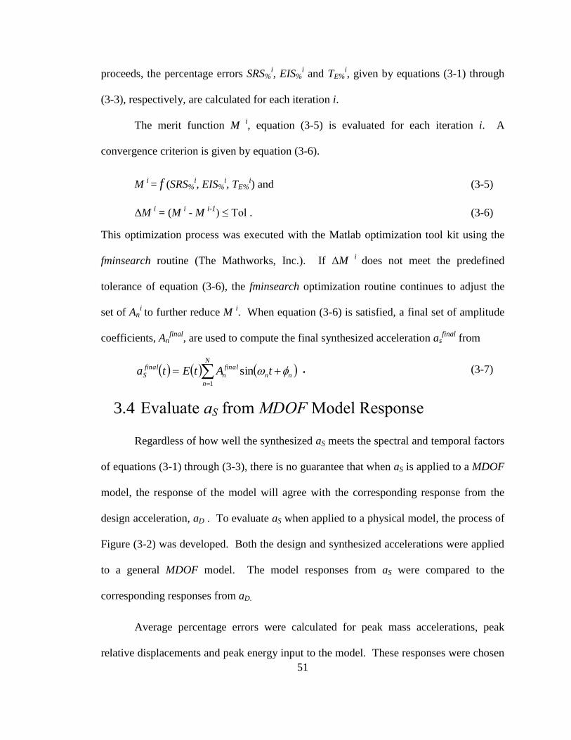
51
proceeds, the percentage errors SRS%i, EIS%
i and TE%
i, given by equations (3-1) through
(3-3), respectively, are calculated for each iteration i.
The merit function M i, equation (3-5) is evaluated for each iteration i. A
convergence criterion is given by equation (3-6).
M i = f (SRS%
i, EIS%
i, TE%
i) and (3-5)
ΔM i = (M
i - M
i-1) ≤ Tol . (3-6)
This optimization process was executed with the Matlab optimization tool kit using the
fminsearch routine (The Mathworks, Inc.). If ΔM i
does not meet the predefined
tolerance of equation (3-6), the fminsearch optimization routine continues to adjust the
set of Ani to further reduce M
i. When equation (3-6) is satisfied, a final set of amplitude
coefficients, Anfinal
, are used to compute the final synthesized acceleration asfinal
from
. (3-7)
3.4 Evaluate aS from MDOF Model Response
Regardless of how well the synthesized aS meets the spectral and temporal factors
of equations (3-1) through (3-3), there is no guarantee that when aS is applied to a MDOF
model, the response of the model will agree with the corresponding response from the
design acceleration, aD . To evaluate aS when applied to a physical model, the process of
Figure (3-2) was developed. Both the design and synthesized accelerations were applied
to a general MDOF model. The model responses from aS were compared to the
corresponding responses from aD.
Average percentage errors were calculated for peak mass accelerations, peak
relative displacements and peak energy input to the model. These responses were chosen
N
n
nn
final
n
final
S tAtEta1
sin
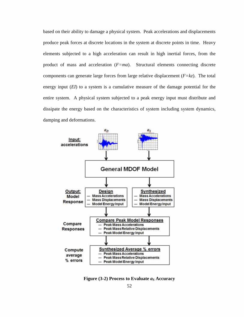
52
based on their ability to damage a physical system. Peak accelerations and displacements
produce peak forces at discrete locations in the system at discrete points in time. Heavy
elements subjected to a high acceleration can result in high inertial forces, from the
product of mass and acceleration (F=ma). Structural elements connecting discrete
components can generate large forces from large relative displacement (F=kz). The total
energy input (EI) to a system is a cumulative measure of the damage potential for the
entire system. A physical system subjected to a peak energy input must distribute and
dissipate the energy based on the characteristics of system including system dynamics,
damping and deformations.
Figure (3-2) Process to Evaluate aS Accuracy

53
A general 3DOF model, Figure (3-3), was developed to evaluate the response of
the synthesized base accelerations relative to that of the design acceleration. This 3DOF
model represents a general system where masses and spring rates were sized to result in
natural frequencies in the range of interest relative to the magnitudes of SRSD and EISD
over the frequency bandwidth. The absolute displacements of masses m1, m2 and m3 are
given by u1, u2 and u3, respectively. Since the excitation of interest is a base acceleration,
a base coordinate ub is defined. A relative coordinates is defined for each mass mi, given
by (ui - ub). Three springs of stiffness k1, k2 and k3 connect the mass elements, and k1
connects mass m1 to the base. The model excitation is a base acceleration, which is the
second time derivative of the base coordinate ub. Damping of ζ = 5% of critical damping
was prescribed for the entire model.
Three variants of the general 3DOF model were developed based on three sets of
spring force-displacement relationships given by,
Linear: linear force-displacement relationship for all springs,
Nonlinear-Stiffening: nonlinear elastic springs where each spring rate
increases when the displacement exceeds a predefined value and
Nonlinear-Softening: nonlinear elastic springs where each spring rate
decreases when the displacement exceeds a predefined value.
Details of the general 3DOF model parameters are given in Appendix B.
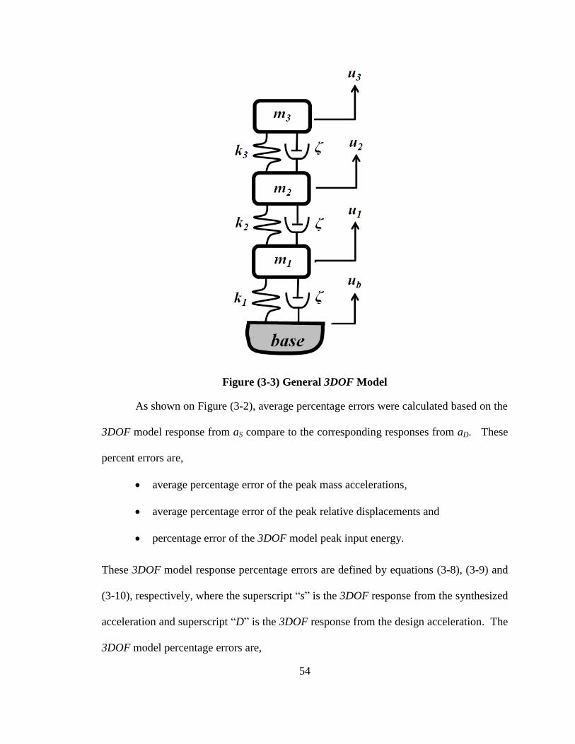
54
Figure (3-3) General 3DOF Model
As shown on Figure (3-2), average percentage errors were calculated based on the
3DOF model response from aS compare to the corresponding responses from aD. These
percent errors are,
average percentage error of the peak mass accelerations,
average percentage error of the peak relative displacements and
percentage error of the 3DOF model peak input energy.
These 3DOF model response percentage errors are defined by equations (3-8), (3-9) and
(3-10), respectively, where the superscript “s” is the 3DOF response from the synthesized
acceleration and superscript “D” is the 3DOF response from the design acceleration. The
3DOF model percentage errors are,
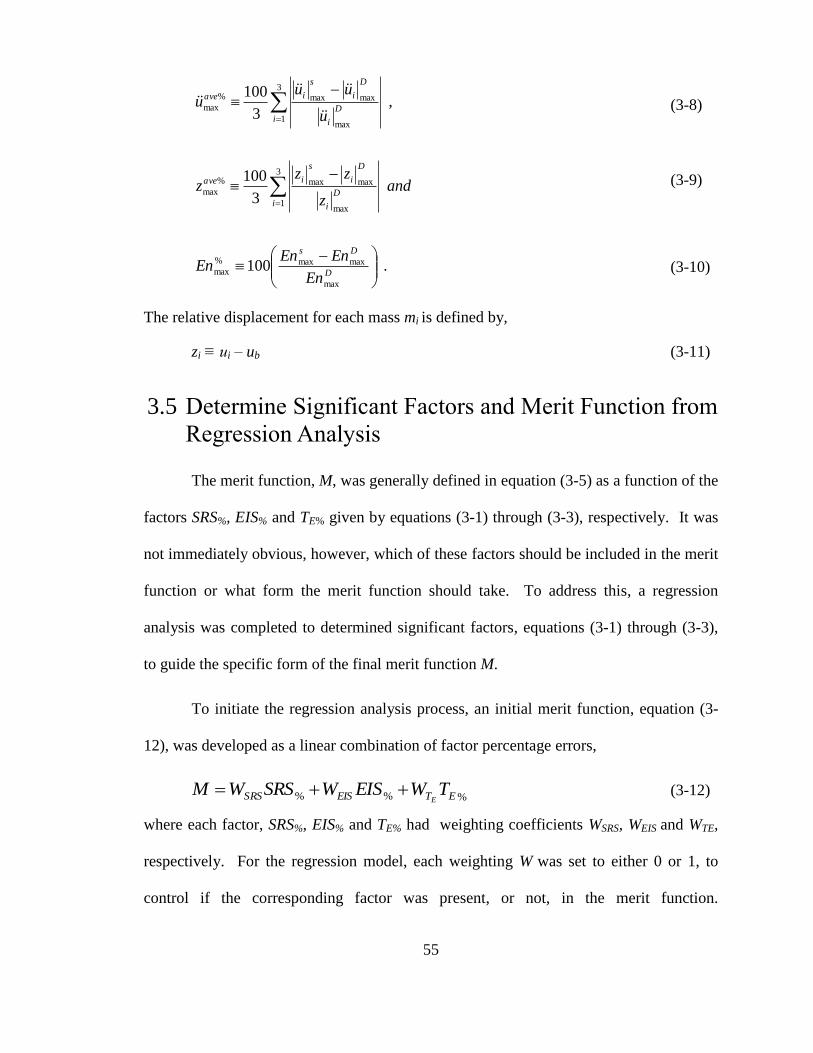
55
(3-8)
(3-9)
(3-10)
The relative displacement for each mass mi is defined by,
zi ≡ ui – ub (3-11)
3.5 Determine Significant Factors and Merit Function from
Regression Analysis
The merit function, M, was generally defined in equation (3-5) as a function of the
factors SRS%, EIS% and TE% given by equations (3-1) through (3-3), respectively. It was
not immediately obvious, however, which of these factors should be included in the merit
function or what form the merit function should take. To address this, a regression
analysis was completed to determined significant factors, equations (3-1) through (3-3),
to guide the specific form of the final merit function M.
To initiate the regression analysis process, an initial merit function, equation (3-
12), was developed as a linear combination of factor percentage errors,
(3-12)
where each factor, SRS%, EIS% and TE% had weighting coefficients WSRS, WEIS and WTE,
respectively. For the regression model, each weighting W was set to either 0 or 1, to
control if the corresponding factor was present, or not, in the merit function.
%%% ETEISSRS TWEISWSRSWME
.100
3
100
,3
100
max
maxmax%
max
3
1max
maxmax%
max
3
1max
maxmax%
max
D
Ds
iD
i
D
i
s
iave
iD
i
D
i
s
iave
En
EnEnEn
andz
zzz
u
uuu

56
Accordingly, equation (3-12) has three W coefficients and each had two values, resulting
in 23=8 total combinations. Each combination of weightings yields a unique aS. With all
combinations of W, eight unique aS base accelerations were synthesized. Table (3-1)
gives the nomenclature for each synthesized acceleration based on Wi values (0 or 1).
The eight synthesized accelerations are plotted in Figure (3-4). The percent error factors
(SRS%, EIS%, TE%) in the merit equation (3-12) were determined for each aS and were the
inputs factors for the regression analysis.
Table (3-1) Synthesized Acceleration Nomenclature base on M Weighting
synthesized
accelerations
WSRS WEIS WTE
as000
0 0 0
as010
0 1 0
as001
0 0 1
as011
0 1 1
as100
1 0 0
as110
1 1 0
as101
1 0 1
as111
1 1 1
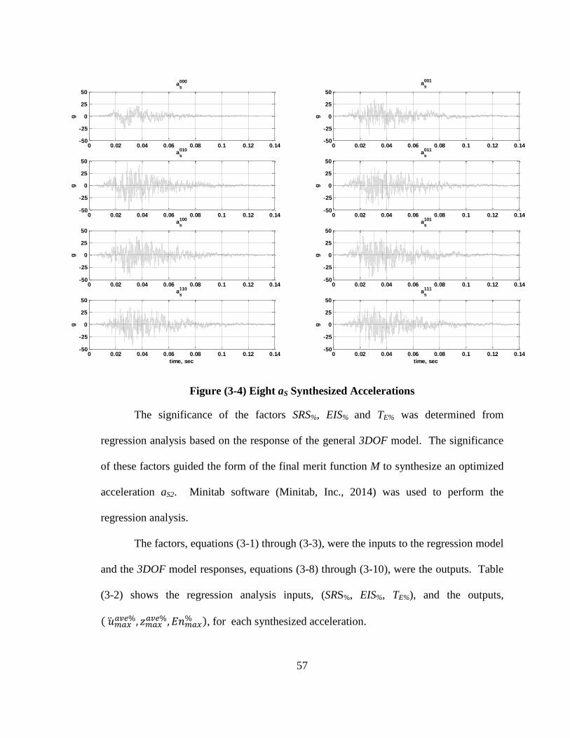
57
Figure (3-4) Eight aS Synthesized Accelerations
The significance of the factors SRS%, EIS% and TE% was determined from
regression analysis based on the response of the general 3DOF model. The significance
of these factors guided the form of the final merit function M to synthesize an optimized
acceleration aS2. Minitab software (Minitab, Inc., 2014) was used to perform the
regression analysis.
The factors, equations (3-1) through (3-3), were the inputs to the regression model
and the 3DOF model responses, equations (3-8) through (3-10), were the outputs. Table
(3-2) shows the regression analysis inputs, (SRS%, EIS%, TE%), and the outputs,
( �̈�𝑚𝑎𝑥𝑎𝑣𝑒%, 𝑧𝑚𝑎𝑥
𝑎𝑣𝑒%, 𝐸𝑛𝑚𝑎𝑥% ), for each synthesized acceleration.
0 0.02 0.04 0.06 0.08 0.1 0.12 0.14-50
-25
0
25
50
as
000
g
0 0.02 0.04 0.06 0.08 0.1 0.12 0.14-50
-25
0
25
50
as
001
g
0 0.02 0.04 0.06 0.08 0.1 0.12 0.14-50
-25
0
25
50
as
010
g
0 0.02 0.04 0.06 0.08 0.1 0.12 0.14-50
-25
0
25
50
as
011
g
0 0.02 0.04 0.06 0.08 0.1 0.12 0.14-50
-25
0
25
50
as
100
g
0 0.02 0.04 0.06 0.08 0.1 0.12 0.14-50
-25
0
25
50
as
101
g
0 0.02 0.04 0.06 0.08 0.1 0.12 0.14-50
-25
0
25
50
as
110
time, sec
g
0 0.02 0.04 0.06 0.08 0.1 0.12 0.14-50
-25
0
25
50
as
111
time, sec
g
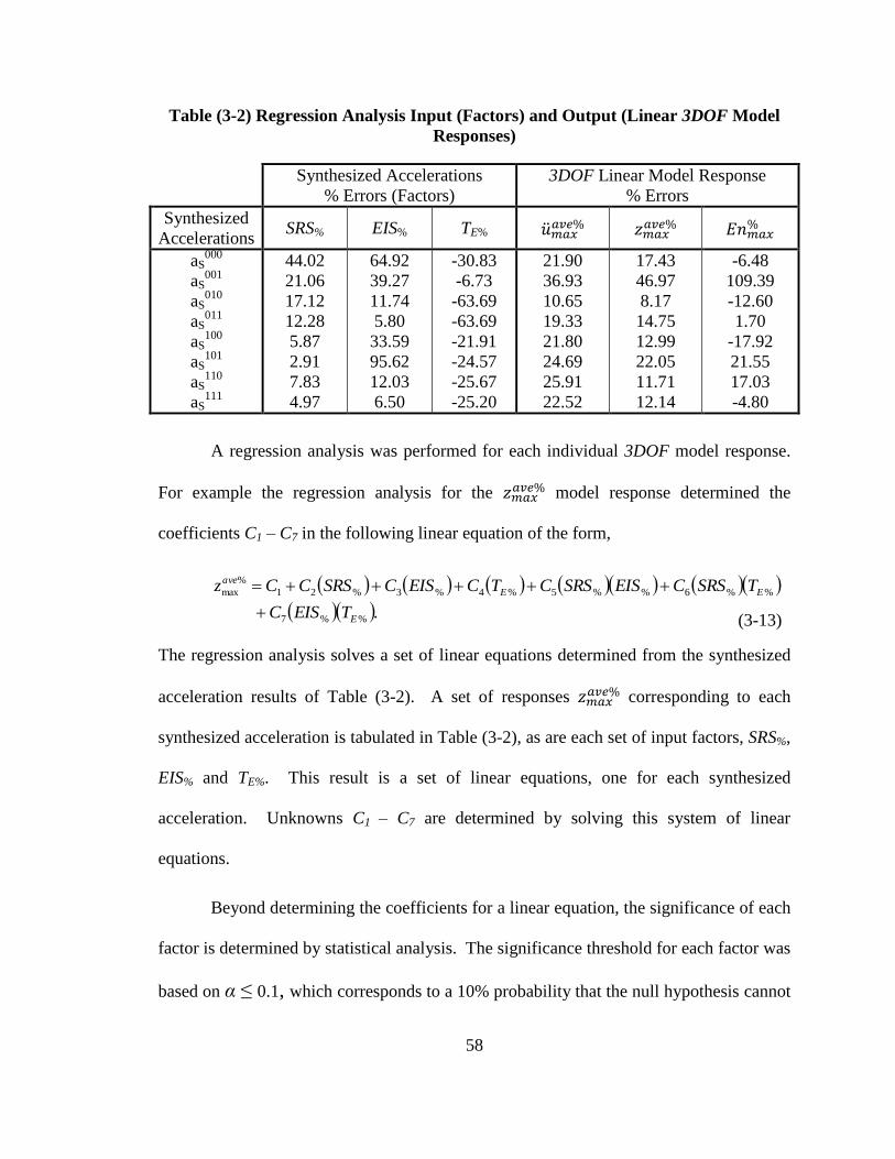
58
Table (3-2) Regression Analysis Input (Factors) and Output (Linear 3DOF Model
Responses)
Synthesized Accelerations
% Errors (Factors)
3DOF Linear Model Response
% Errors
Synthesized
Accelerations SRS% EIS% TE% �̈�𝑚𝑎𝑥
𝑎𝑣𝑒% 𝑧𝑚𝑎𝑥𝑎𝑣𝑒% 𝐸𝑛𝑚𝑎𝑥
%
aS000
aS001
aS010
aS011
aS100
aS101
aS110
aS111
44.02
21.06
17.12
12.28
5.87
2.91
7.83
4.97
64.92
39.27
11.74
5.80
33.59
95.62
12.03
6.50
-30.83
-6.73
-63.69
-63.69
-21.91
-24.57
-25.67
-25.20
21.90
36.93
10.65
19.33
21.80
24.69
25.91
22.52
17.43
46.97
8.17
14.75
12.99
22.05
11.71
12.14
-6.48
109.39
-12.60
1.70
-17.92
21.55
17.03
-4.80
A regression analysis was performed for each individual 3DOF model response.
For example the regression analysis for the 𝑧𝑚𝑎𝑥𝑎𝑣𝑒% model response determined the
coefficients C1 – C7 in the following linear equation of the form,
(3-13)
The regression analysis solves a set of linear equations determined from the synthesized
acceleration results of Table (3-2). A set of responses 𝑧𝑚𝑎𝑥𝑎𝑣𝑒% corresponding to each
synthesized acceleration is tabulated in Table (3-2), as are each set of input factors, SRS%,
EIS% and TE%. This result is a set of linear equations, one for each synthesized
acceleration. Unknowns C1 – C7 are determined by solving this system of linear
equations.
Beyond determining the coefficients for a linear equation, the significance of each
factor is determined by statistical analysis. The significance threshold for each factor was
based on α ≤ 0.1, which corresponds to a 10% probability that the null hypothesis cannot
.%%7
%%6%%5%4%3%21
%
max
E
EE
ave
TEISC
TSRSCEISSRSCTCEISCSRSCCz
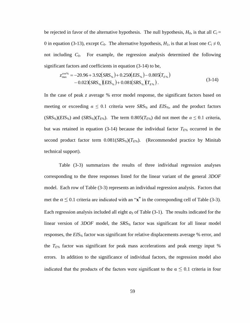
59
be rejected in favor of the alternative hypothesis. The null hypothesis, H0, is that all Ci =
0 in equation (3-13), except C0. The alternative hypothesis, H1, is that at least one Ci ≠ 0,
not including C0. For example, the regression analysis determined the following
significant factors and coefficients in equation (3-14) to be,
(3-14)
In the case of peak z average % error model response, the significant factors based on
meeting or exceeding α ≤ 0.1 criteria were SRS% and EIS%, and the product factors
(SRS%)(EIS%) and (SRS%)(TE%). The term 0.805(TE%) did not meet the α ≤ 0.1 criteria,
but was retained in equation (3-14) because the individual factor TE% occurred in the
second product factor term 0.081(SRS%)(TE%). (Recommended practice by Minitab
technical support).
Table (3-3) summarizes the results of three individual regression analyses
corresponding to the three responses listed for the linear variant of the general 3DOF
model. Each row of Table (3-3) represents an individual regression analysis. Factors that
met the α ≤ 0.1 criteria are indicated with an “x” in the corresponding cell of Table (3-3).
Each regression analysis included all eight aS of Table (3-1). The results indicated for the
linear version of 3DOF model, the SRS% factor was significant for all linear model
responses, the EIS% factor was significant for relative displacements average % error, and
the TE% factor was significant for peak mass accelerations and peak energy input %
errors. In addition to the significance of individual factors, the regression model also
indicated that the products of the factors were significant to the α ≤ 0.1 criteria in four
.081.0023.0
805.0250.092.396.20
%%%%
%%%
%
max
E
E
ave
TSRSEISSRS
TEISSRSz
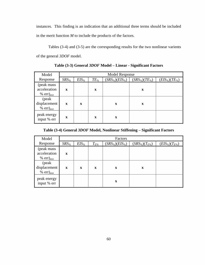
60
instances. This finding is an indication that an additional three terms should be included
in the merit function M to include the products of the factors.
Tables (3-4) and (3-5) are the corresponding results for the two nonlinear varients
of the general 3DOF model.
Table (3-3) General 3DOF Model – Linear - Significant Factors
Model
Response
Model Response
SRS% EIS% TE% (SRS%)(EIS%) (SRS%)(TE%) (EIS%)(TE%)
(peak mass
acceleration
% err)ave x x x
(peak
displacement
% err)ave x x x x
peak energy
input % err x x x
Table (3-4) General 3DOF Model, Nonlinear Stiffening – Significant Factors
Model
Response
Factors
SRS% EIS% TE% (SRS%)(EIS%) (SRS%)(TE%) (EIS%)(TE%)
(peak mass
acceleration
% err)ave x
(peak
displacement
% err)ave x x x x x
peak energy
input % err x
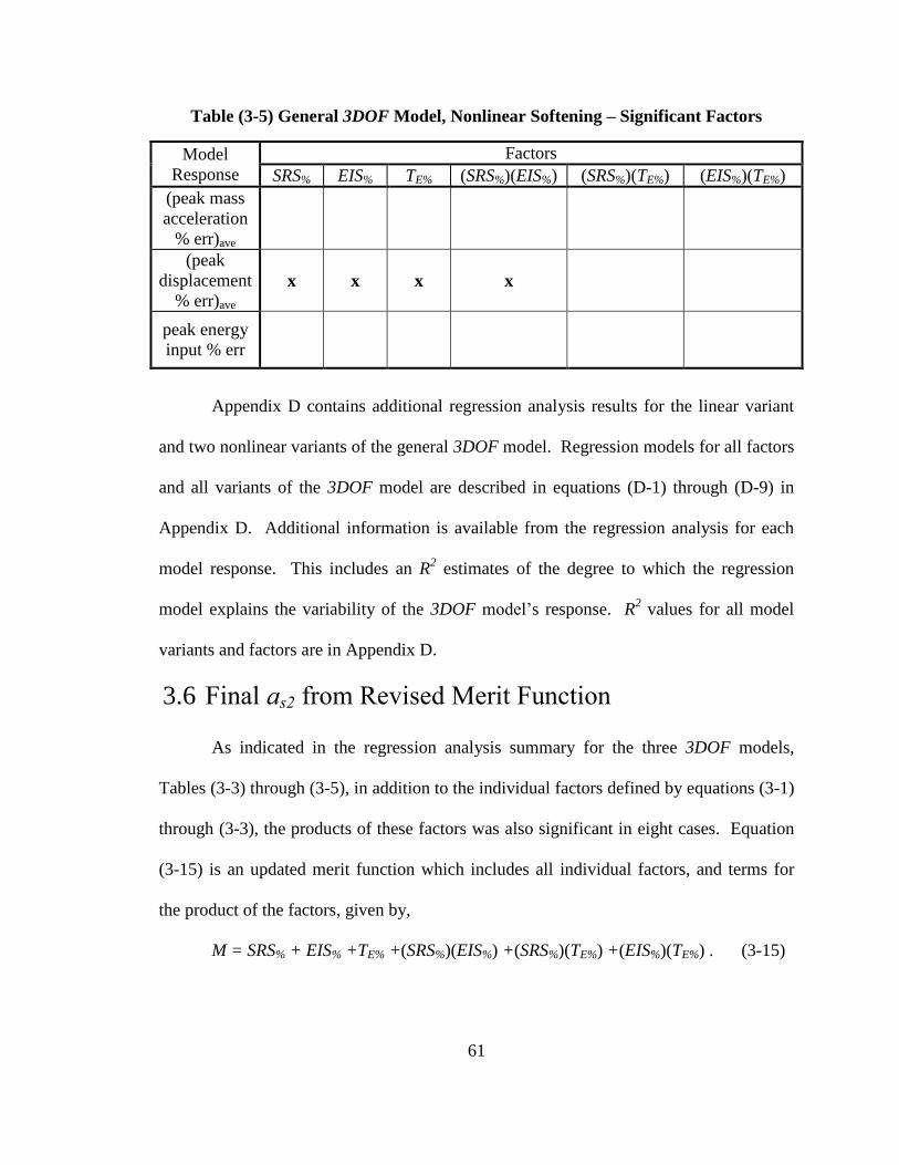
61
Table (3-5) General 3DOF Model, Nonlinear Softening – Significant Factors
Model
Response
Factors
SRS% EIS% TE% (SRS%)(EIS%) (SRS%)(TE%) (EIS%)(TE%)
(peak mass
acceleration
% err)ave
(peak
displacement
% err)ave x x x x
peak energy
input % err
Appendix D contains additional regression analysis results for the linear variant
and two nonlinear variants of the general 3DOF model. Regression models for all factors
and all variants of the 3DOF model are described in equations (D-1) through (D-9) in
Appendix D. Additional information is available from the regression analysis for each
model response. This includes an R2 estimates of the degree to which the regression
model explains the variability of the 3DOF model’s response. R2 values for all model
variants and factors are in Appendix D.
3.6 Final as2 from Revised Merit Function
As indicated in the regression analysis summary for the three 3DOF models,
Tables (3-3) through (3-5), in addition to the individual factors defined by equations (3-1)
through (3-3), the products of these factors was also significant in eight cases. Equation
(3-15) is an updated merit function which includes all individual factors, and terms for
the product of the factors, given by,
M = SRS% + EIS% +TE% +(SRS%)(EIS%) +(SRS%)(TE%) +(EIS%)(TE%) . (3-15)
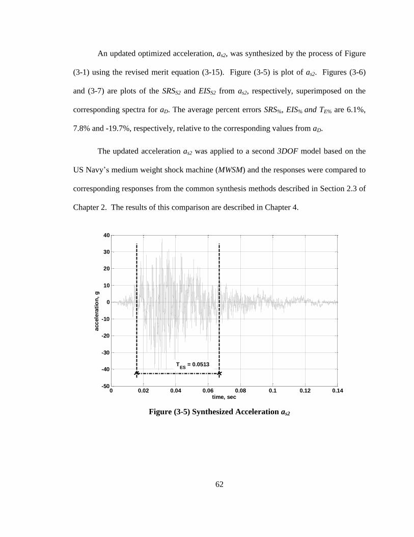
62
An updated optimized acceleration, as2, was synthesized by the process of Figure
(3-1) using the revised merit equation (3-15). Figure (3-5) is plot of as2. Figures (3-6)
and (3-7) are plots of the SRSS2 and EISS2 from as2, respectively, superimposed on the
corresponding spectra for aD. The average percent errors SRS%, EIS% and TE% are 6.1%,
7.8% and -19.7%, respectively, relative to the corresponding values from aD.
The updated acceleration as2 was applied to a second 3DOF model based on the
US Navy’s medium weight shock machine (MWSM) and the responses were compared to
corresponding responses from the common synthesis methods described in Section 2.3 of
Chapter 2. The results of this comparison are described in Chapter 4.
Figure (3-5) Synthesized Acceleration as2
0 0.02 0.04 0.06 0.08 0.1 0.12 0.14-50
-40
-30
-20
-10
0
10
20
30
40
time, sec
acc
ele
rati
on
, g
TES
= 0.0513
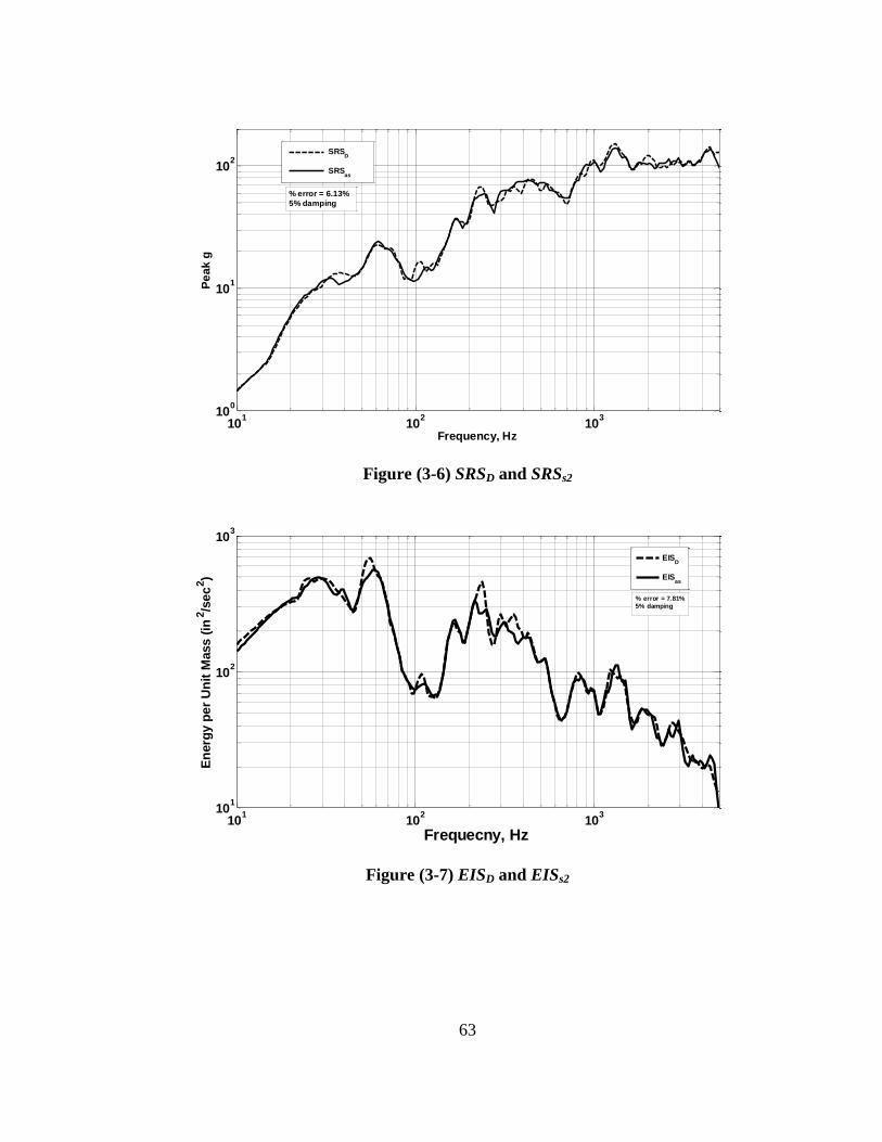
63
Figure (3-6) SRSD and SRSs2
Figure (3-7) EISD and EISs2
101
102
103
100
101
102
Frequency, Hz
Pe
ak
g
SRSD
SRSas
% error = 6.13%
5% damping
101
102
103
101
102
103
Frequecny, Hz
En
erg
y p
er
Un
it M
ass
(in
2/s
ec
2)
EISD
EISas
% error = 7.81%
5% damping
64
4 Multi-degree of Freedom Response
to Synthesized Accelerations
4.1 Overview
A design SRSD and EISD were developed from the design acceleration aD, Figures
(2-14) and (2-13), respectively. Five accelerations aS were synthesized to be compatible
with SRSD, Figure (4-1). Four of the five (half sine, damped sines, wavelets, enveloped
sines) were synthesized with current industry practices, which is to achieve the best
match between SRSS and SRSD, as shown in Figure (2-8). The fifth acceleration, aS2, was
synthesized to match not only SRSD, but also the design energy input spectrum (EISD),
design duration (TED) and the design envelope function E(t). Three 3DOF medium
weight shock machine (MWMS) models were developed to evaluate the differences
between the 3DOF MWSM model responses from five aS relative to the corresponding
MWSM model response to aD.
4.2 Synthesized Accelerations Evaluated
As described in Chapter 3, as2 was synthesized to minimize the SRS, EIS and TE
percentage error factors defined by equations (3-1) through (3-3). The minimization was
done using the updated merit function of equation (3-15). Four other synthesized
accelerations, described in Chapter 2, were synthesized based on common industry
practice to only minimize SRSS percent error defined by equation (3-1). Figure (4-1)
contains plots of the design acceleration aD, the four synthesized accelerations of Figure
(2-7), and aS2 of Figure (3-5). Note that the time scale of the half sine plot on Figure (4-
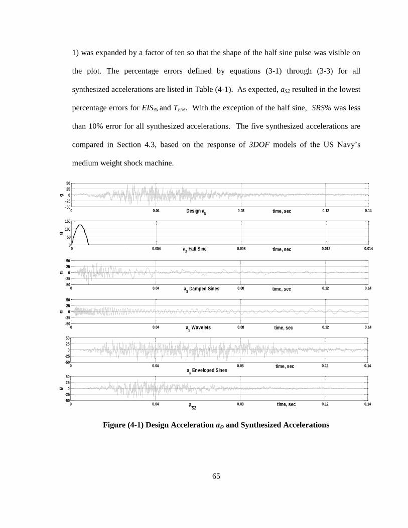
65
1) was expanded by a factor of ten so that the shape of the half sine pulse was visible on
the plot. The percentage errors defined by equations (3-1) through (3-3) for all
synthesized accelerations are listed in Table (4-1). As expected, aS2 resulted in the lowest
percentage errors for EIS% and TE%. With the exception of the half sine, SRS% was less
than 10% error for all synthesized accelerations. The five synthesized accelerations are
compared in Section 4.3, based on the response of 3DOF models of the US Navy’s
medium weight shock machine.
Figure (4-1) Design Acceleration aD and Synthesized Accelerations
0 0.04 0.08 0.12 0.14-50
-25
0
25
50
aS2
time, sec
g
0 0.04 0.08 0.12 0.14-50
-25
0
25
50
Design aD
g
time, sec
0 0.004 0.008 0.012 0.0140
50
100
150
aS Half Sine
g
time, sec
0 0.04 0.08 0.12 0.14-50
-25
0
25
50
aS Damped Sines
g
time, sec
0 0.04 0.08 0.12 0.14-50
-25
0
25
50
aS Wavelets
g
time, sec
0 0.04 0.08 0.12 0.14-50
-25
0
25
50
as Enveloped Sines
time, sec
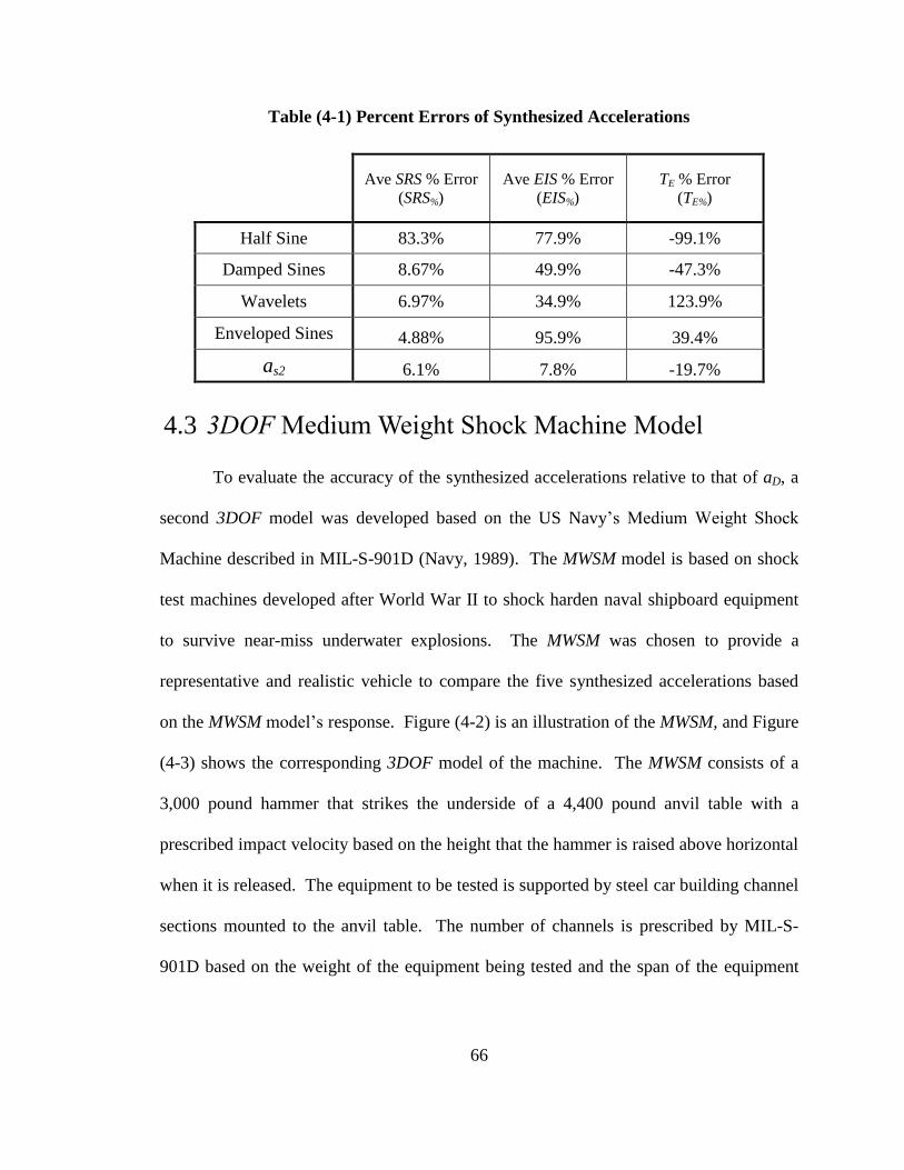
66
Table (4-1) Percent Errors of Synthesized Accelerations
Ave SRS % Error
(SRS%)
Ave EIS % Error
(EIS%)
TE % Error
(TE%)
Half Sine 83.3% 77.9% -99.1%
Damped Sines 8.67% 49.9% -47.3%
Wavelets 6.97% 34.9% 123.9%
Enveloped Sines 4.88% 95.9% 39.4%
as2 6.1% 7.8% -19.7%
4.3 3DOF Medium Weight Shock Machine Model
To evaluate the accuracy of the synthesized accelerations relative to that of aD, a
second 3DOF model was developed based on the US Navy’s Medium Weight Shock
Machine described in MIL-S-901D (Navy, 1989). The MWSM model is based on shock
test machines developed after World War II to shock harden naval shipboard equipment
to survive near-miss underwater explosions. The MWSM was chosen to provide a
representative and realistic vehicle to compare the five synthesized accelerations based
on the MWSM model’s response. Figure (4-2) is an illustration of the MWSM, and Figure
(4-3) shows the corresponding 3DOF model of the machine. The MWSM consists of a
3,000 pound hammer that strikes the underside of a 4,400 pound anvil table with a
prescribed impact velocity based on the height that the hammer is raised above horizontal
when it is released. The equipment to be tested is supported by steel car building channel
sections mounted to the anvil table. The number of channels is prescribed by MIL-S-
901D based on the weight of the equipment being tested and the span of the equipment

67
mounting attachment locations. The intent is to achieve a system frequency equivalent to
the frequency of the deck of the ship where the equipment is to be mounted.
Figure (4-2) Illustration of Medium Weight Shock Machine
Figure (4-3) 3DOF Model of Medium Weight Shock Machine
As shown in Figure (4-3), spring stiffness k1 is the combined stiffness of the
mounting channels. Spring k2 represents the combined stiffness of four commercial
68
shock absorbers, and spring k3 represents the stiffness of the chassis of the equipment
being tested. In this model stiffness k2 is based on a commercial shock isolator described
in Appendix C. Springs k1 and k3 are linear for all variants of the MWSM model. As with
the general 3DOF model described in Chapter 3, the MWSM model has three variants;
linear, nonlinear-stiffening and nonlinear-softening based on the force-displacement
relationship of k2. The MWSM model damping was set to 5% of critical based on
historical data taken at the Naval Research Lab (Clements, 1972).
4.4 MWSM Model Response to Synthesized Accelerations
MWSM model percentage error responses from the synthesized accelerations
relative to those of aD are plotted in Figures (4-4), (4-5) and (4-6) for the linear,
nonlinear-stiffening and nonlinear-softening model variants, respectively. These
percentage errors correspond to those defined by equations (3-8), (3-9) and (3-10) for
average peak mass accelerations, average peak displacements and peak energy input to
the model, respectively.
For the linear MWSM model, the errors from aS2 were lower than the
corresponding errors from the other synthesized accelerations for all model responses,
Figure (4-4). Model response errors from the half-sine had the greatest magnitude, which
is not unexpected due to the significant difference in the half-sine transient pulse
compared to that of aD. Percentage errors from the other three synthesized accelerations
(damped sines, wavelets, and enveloped sines, respectively) were relatively low for peak
accelerations and displacements, although still greater than those corresponding to aS2.
The most significant difference in model response was that of the peak input energy
69
percent error. The average magnitude of En%
max from aS2 was 8.4% compared to an
average magnitude error of 51% for the other four synthesized accelerations.
The same trend was observed from the two nonlinear variants of the MWSM
model responses. The half-sine again had significantly larger errors for peak
accelerations, peak displacements and energy input. The other synthesized accelerations,
including aS2, had comparable percentage errors for peak accelerations and
displacements. However, aS2 again had consistently lower energy input percent errors,
En%
max, in all cases. The merit function to synthesize aS2, equation (3-15), included the
energy input spectrum error term EIS%. This translated to the lowest model input energy
percent error, En%
max, from aS2 relative to the other synthesized accelerations, which were
synthesized to match SRSD only.
Peak mass acceleration and the peak relative displacement responses occur at
specific locations in the system at a discrete point in time during the transient. A peak
mass acceleration will affect the inertial force on an individual component at a specific
location in the system. A peak relative displacement will affect a connecting spring
element in the system that transmits a dynamic force between two mass components.
Spring elements occur at specific locations and the spring forces occur at discrete
instances in time. Peak energy input is a measure to the total energy absorbed by the
entire structural dynamic system. As such, energy input is an appropriate measure of
total damage potential to the structural system. As noted by Edwards (2007):
“The energy quantities can be calculated for MDOF structures by integrating the
energy equations over the entire structure. The results represent the total input,
absorbed, dissipated and kinetic energy of the MDOF structure. On the other
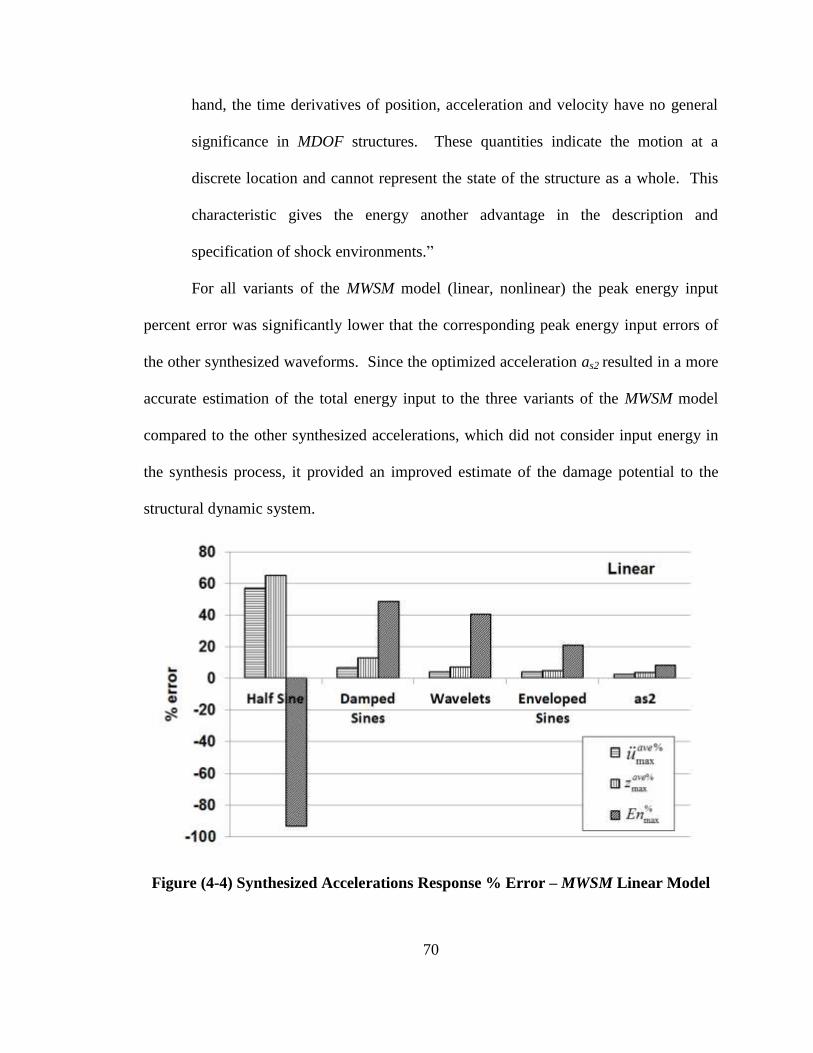
70
hand, the time derivatives of position, acceleration and velocity have no general
significance in MDOF structures. These quantities indicate the motion at a
discrete location and cannot represent the state of the structure as a whole. This
characteristic gives the energy another advantage in the description and
specification of shock environments.”
For all variants of the MWSM model (linear, nonlinear) the peak energy input
percent error was significantly lower that the corresponding peak energy input errors of
the other synthesized waveforms. Since the optimized acceleration as2 resulted in a more
accurate estimation of the total energy input to the three variants of the MWSM model
compared to the other synthesized accelerations, which did not consider input energy in
the synthesis process, it provided an improved estimate of the damage potential to the
structural dynamic system.
Figure (4-4) Synthesized Accelerations Response % Error – MWSM Linear Model
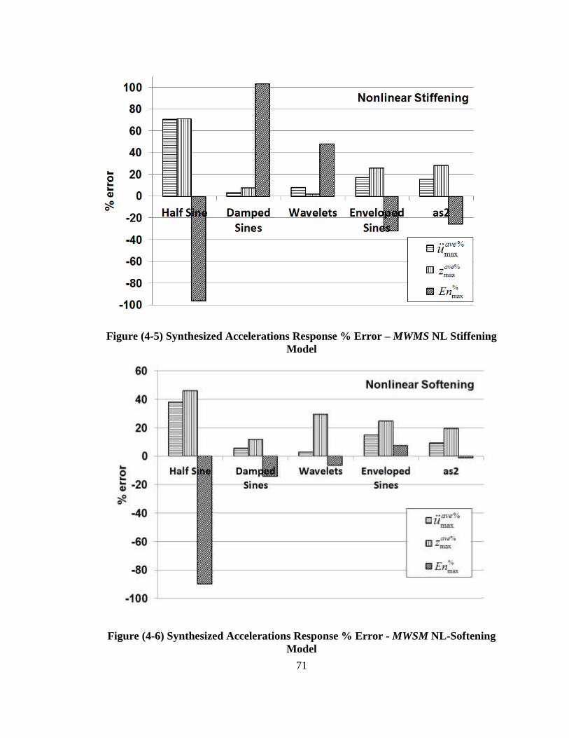
71
Figure (4-5) Synthesized Accelerations Response % Error – MWMS NL Stiffening
Model
Figure (4-6) Synthesized Accelerations Response % Error - MWSM NL-Softening
Model
72
5 Conclusions and Recommendations
The SRS has been in existence for eight decades and has achieved worldwide
acceptance since inception, especially subsequent to the advent of digital computing.
Defense, aerospace and commercial nuclear power communities all have structural
dynamic environment design requirements based on a design SRSD. The SRS provides a
compact SDOF frequency response based measure of a transient acceleration, and with
mode superposition can be leveraged to estimate the maximum response of a linear
MDOF system. The SRS is used to characterize the shock environment for both
structural dynamic analysis and testing.
However, despite the popularity of the SRS, significant limitations exist. The SRS
is a linear transform and cannot be used directly for structural dynamic analyses of
nonlinear MDOF structures or structural testing. The controller of an electro-dynamic
test machine cannot drive the armature of the shaker table directly from an SRS signal.
For both nonlinear analysis and testing, an SRS compatible transient acceleration signal is
required. These limitations motivated researchers to solve the inverse problem; namely
to synthesize a transient acceleration signal that is compatible with a prescribed design
SRSD. However, the SRS forward linear transform process retains no phasing or temporal
information from the transient acceleration time signal. While a shock acceleration time
history will transform to a unique SRS, the inverse is not true. There are theoretically an
infinite number of shock accelerations aS which can be synthesized to be compatible with
a prescribed SRS. As such, SRS compatible synthesized accelerations can be significantly
dissimilar in overall envelope shapes, temporal durations, peak amplitudes and phasing of
73
the sinusoids relative to the original acceleration. “Manufactured” signals have been
published that exhibit curious temporal shapes which have little relation to physical data,
but nonetheless are compatible with the prescribed SRS.
It is not difficult to synthesize an SRSD compatible base acceleration with good
accuracy. Numerous methods have been published to do this including classical
acceleration pulses, the summation of sinusoids (damped sines, wavelets, enveloped
sines) and less common techniques such as a trained neural network, maximum entropy
principal and others. While somewhat limited, prior research has indicated that a base
acceleration synthesized to be compatible with only a prescribed SRSD, with no other
constraints, does not in general yield accurate MDOF peak mass accelerations and/or
displacements when compared to known model responses. The research herein has
confirmed this finding. That said, peak mass acceleration and peak mass displacements
at discrete locations in a structure have no general significant for the damage potential of
the structure as a whole. A more appropriate global MDOF response, which includes
energy input to the structure, is a better measure of system damage potential from an
SRSD compatible synthesized acceleration. For these reasons, the constraints to synthesize
a base acceleration, and the corresponding response of an MDOF structure, have been
reevaluated to include additional information. Based on regression analysis, individual
percent error factors of the synthesized acceleration (SRS%, EIS% and TE%) were all
determined to be significant to the α ≤ 0.1 criteria based on the response of general 3DOF
models. The products of the factors were also determined to be significant to the α ≤ 0.1
criteria. A synthesized acceleration optimized to minimize a merit function comprised of

74
these six factors, equation (3-15), resulted in the most accurate energy input to all
variants (linear and nonlinear) of a 3DOF MWSM model.
The research herein motivates expanding the aS synthesis process beyond current
procedures. In addition to synthesis of aS to be compatible with a prescribed SRSD, other
parameters can be included in the process to improve the quality of aS. These parameters
include temporal information (envelope, duration) and the energy input spectrum, EIS.
Based on linear and nonlinear 3DOF model response accuracy, the proposed approach
resulted in peak system accelerations and displacements that were at parity with, if not
better than, current practices. The proposed approach consistently achieved the most
accurate energy input for all variants of a 3DOF model.

75
6 Bibliography
Alexander, J. E. (1995). A Nonlinear DDAM Procedure. SAVIAC Proceedings of the
66th Shock and Vibration Symposium, 1, pp. pp 251-262. Biloxi, MS.
Alexander, J. E. (1998). Structural Analysis of a Nonlinear System Given a Shock
Response Spectrum Input. SAVIAC Proceedings of the 69th Shock and Vibration
Symposium, Unlimited Volume. Minneapolis, MN.
Alexander, J. E. (2009). Shock Response Spectrum - A Primer. Sound and Vibration, Vol
43 / No 6(June), pp 6-15.
Alexander, J. E. (2011). Application of Energy Methods in Mechanical Shock to Study
Base Excited Nonlinear System Response. Conference Proceedings of the Society for
Experimental Mechanics. Vol 5, pp. pp 157-175. Rotating Machinery, Structural Health
Monitoring, Shock and Vibration.
Barry Controls. (n.d.). SLM Mount Series. Retrieved August 15, 2015, from
http://www.barrycontrols.com/userfiles/file/product_catalog/machinery/bcdi_prod_machi
nery_catalog.pdf
Bathe, K., & Gracewski, S. (1981). On Nonlinear Dynamic Analysis Using
Substructuring and Mode Superposition. Computers & Structures, 13, 699-707.
Biot, M. (1932). Transient Oscillations in Elastic Systems. California Institute of
Technology.
Brake, M. R. (2011). An Inverse Shock Response Spectrum. Mechanical Systems and
Signal Processing, 25, 2654-2672.
Bureau of Ships. (1961). Shock Design of Shipboard Equipment, Dynamic Design-
Analysis Method. Navy Department, Bureau of Ships, Washington D.C.
Chang, C. J., & Mohraz, B. (1990). Modal Analysis of Nonlinear Systems with Classical
and Non-Classical Damping. Computers & Structures, 36, 1067-1080.
Clements, E. W. (1972). Shipboard Shock and Navy Devices for its Simulation, NRL
Report 7396. Naval Research Laboratory, Washington, DC.
76
Clough, H. L., & Penzien, J. (1975). In Dynamics of Structures. New York: McGraw
Hill.
Dassault Systemes Simulia Corp. (2008). Abaqus (Version 6.8). Providence, RI.
Department of Defense. (2008). MIL-STD-810G, Environmental Engineering
Considerations and Laboratory Tests. Military Standard.
Department of the Navy, Naval Sea Systems Command. (1972). Design Data Sheet 072-
1, Shock Design Values.
Edwards, T. S. (2007). Using Work and Energy to Characterize Mechanical Shock.
Institute of Environmental Sciences and Technology, Annual Technical Meeting of the
IEST, Conference Proceedings, ISBN: 978-1-60423-442-8, Vol 1, pp. pp 280-298.
Edwards, T. S. (2009). Power Delivered to Mechanical Systems by Random Vibration.
Shock and Vibration, Vol 16, no. 3, pp 261-271.
Gaberson, H. A. (1995). Reasons for Presenting Shock Spectra with Velocity as the
Ordinate. Proceedings of the 66th Shock and Vibration Symposium. SAVIAC.
Gasparini, D., & Vanmarcke, E. H. (Jan 1976). Simulated Earthquake Motions
Compatible with Prescribed Response Spectra. Pub. No. R76-4, Evaluation of Seismic
Safety of Buildings, Report No. 2, MIT, Department of Civil Engineering.
Ghaboussi, J., & Lin, C. C. (1998). New Method of Generating Spectrum Compatible
Accelerograms Using Neural Networks. Earthquake Engineering and Structural
Dynamics, 27, 377-396.
Ghosh, A. K. (1991). On the Generation of Ground Motion Accelerogram Compatible
with a Specified Response Spectrum and a Fourier Amplitude Spectrum. SMiRT 11
Transactions, 11, 7-12.
Gupta, I. D., & Trifunac, M. D. (1998). Defining Equivalent Stationary PSDF to Account
for Nonstationarity of Earthquake Ground Motion. Soil Dynamics and Earthquake
Engineering, 17, 89-99.
Hartwig, T. (2013). Evaluation of Transportation Vibration Associated with Relocation
of Work in Process as Part of KCRIMS. Honeywell, Federal Manufacturing &
Technology, Kansas City, MO.
Housner, G. W. (1947). Characteristics of Strong Motion Earthquakes. Bulletin of the
Seismological Society of America, Vol 37, No 1, pp 19-31.
77
Housner, G. W. (1955, July). Properties of Strong Ground Motion Earthquakes. Bulletin
of the Seismological Society of America, Vol 45, No 3, pp 197-218.
Housner, G. W. (1959). Behavior of Structures During Earthquakes. Journal of the
Engineering Mechanics Division (ASCE), (pp. 109-129).
Housner, G. W., & Jennings, P. C. (1964). Generation of Artificial Earthquakes. Journal
of the Engineering Mechanics Division. Vol 90, pp. pp 113-150. Proceedings of the
ASCE.
Hudson, D. E. (1956). Response Spectrum Techniques in Engineering Seismology.
Proceedings of the World Conference on Earthquake Engineering. Berkeley, CA.
International Test and Evaluation Steering Committee. (2000). FR/GE/UK/US,
International Test Operations Procedure (ITOP) 4-2-828, Ballistic Shock Testing.
Irvine, T. (2015, June 24). SHOCK AND VIBRATION RESPONSE SPECTRA COURSE
Unit 29. Shock Response Spectrum Synthesis via Wavelets. Retrieved 2015, from
http://www.vibrationdata.com/Course_Units/UNIT29.pdf.
Iwasa, T., Shi, Q., & Saitoh, M. (2008). Shock Response Spectrum Based on Maximum
Total Energy of Single Degree of Freedom Model. AIAA 2008-1742, 49th Structural
Dynamics and Materials Conference. Schaumburg, IL.: AIAA/ASME/ASCE/ASC
Structures.
Iyengar, R. N., & Iyengar, K. T. (1969, June). Nonstationary Random ProcessModel for
Warthquake Accelerograms. Bulletin of the Seismological Society of America, 59 (3), pp.
1163-1188.
Iyengar, R. N., & Rao, P. N. (1979). Generation of Spectrum Compatible Accelerograms.
Earthquake Engineering and Structural Dynamics, 7, 253-263.
Jennings, P. C., Housner, G. W., & Tsai, N. C. (1968). Simulated Earthquake Motions.
California Institute of Technology , Earthquake Engineering Research Laboratory,
Pasadena.
Kost, G., Tellkamp, T., Gantayat, A., & Weber, F. (1978). Automated Generation of
Spectrum-Compatible Artificial Time Histories. Nuclear Engineering and Design, 45,
243-249.
Kukreti, A. R., & Issa, H. I. (1984). Dynamic Analysis of Nonlinear Structures by
Pseudo-Normal Mode Superposition Method. Computers & Structures, 19, 653-663.

78
Lee, S. C., & Han, S. W. (2010). Neural Network Based Models for Generating Artificial
Earthquakes and Response Spectra. Computers and Structures, 80, 1627-1638.
Levy, S., & Wilkinson, J. P. (1976). Generation of Artificial Time-Hiostories, Rich in All
Frequencies, From Given Response Spectra. Nuclear Engineering and Design, 38, 241-
251.
Lin, Y., & Sun, T. (1993). Mode Superposition Analysis of Viscously Damped Nonlinear
Structural Systems Using an Incremental Algorithm. Journal of Vibration and Acoustics,
Transactions of the ASME, 115, 397-402.
Manfredi, G. (2001). Evaluation of Seismic Energy Demand. Earthquake Engineering
and Structural Dynamics, Vol 30, pp 485-499.
(2008). MIL-STD-810G, Method 516.6, Shock. Department of Defense, Test Method
Standard - Environmental Engineering Considerations and Labortaory Tests.
Ministry of Defense. (2006). Environmental Handbood for Defence Materiel, Part 3,
Envirohmental Test Methods, DEF STAN 00-35 Part 3 Issue 4. MOD.
Minitab, Inc. (2014, April). Minitab (version 16). State College, PA.
NASA. (1999). Pyroshock Test Criteria, NASA Technical Standard, NASA-STD-7003.
NASA.
NASA. (2001). Dynamic Environmental Criteria, NASA-HDBK-7005. NASA Technical
Handbook.
Navy, U. S. (1989). MIL-S-901D .
Nelson, D. B. (1989). Parameter Specification for Shaker Shock Waveform Synthesis -
Damped Sines and Wavelets. 60th Shock and Vibration Symposium. III, pp. 151-193.
Portsmouth: Shock and Vibration Information Analysis Center (SAVIAC).
Newmark, N. M., Blume, J. A., & Kapur, K. K. (1973). Design Response Spectra for
Nuclear Power Plants. American Society of Civil Engineers (ASCE) Structural
Engineering Meeting (pp. 287-303). San Francisco: ASCE.
O'Hara, G. J., & Belsheim, R. O. (Feb, 1963). Interim Design Values for Shock Design of
Shipboard Equipment, NRL Memorandum Report 1396. U. S. Naval Research
Laboratory.

79
Ordaz, M., Huerta, B., & Reinoso, E. (2003). Exact Computation of Input-Energy Spectra
from Fourier Amplitude Spectra. Earthquake Engineering and Structural Dynamics, 32,
597-605.
Preumont, A. (1980). A Method for the Generation of Artificial Earthquake
Accelerograms. Nuclear Engineering and Design, 59, 357-368.
Preumont, A. (1984). The Generation of Spectrum Compatible Accelerograms for the
Desigh of Nuclear Power Plants. Earthquake Engineering and Structural Dynamics, 12,
481-497.
Rizzo, P. C., Shaw, D. E., & Jarecki, S. J. (1973). Development of Real/Synthesized
Time Histories to Match Smooth Design Spectra. Berlin: International Conference on
Structural Mechanics in Reactor Technology.
Saragoni, G. R., & Hart, G. C. (1974). Simulation of Artificial Earthquakes. Earthquake
Engineering and Structural Dynamics, 2, 249-267.
Scanlan, R. H., & Sachs, K. (1974). Earthquake Time Histories and Response Spectra.
Journal of the Engineering Mechanics Division. 100, pp. 635-655. American Society of
Civil Engineering.
Shah, V. N., Bohm, G. J., & Nahavandi, A. N. (1979). Modal Superposition Method for
Computationally Economical Nonlinear Structural analysis. 101, pp. 134-141. Montreal:
Transactions of the ASME.
Shinozuka, M. (1973). Digital Simulation of Ground Accelerations. 5th World
Conference of Earthquake Engineering, (pp. 2829-2838). Rome.
Smallwood, D. O. (1986). Shock Testing on Shakers by Using Digital Control. Institute
of Environmental Sciences. Mount Prospect: Institute of Environmental Sciences.
Smallwood, D. O., & Nord, A. R. (1974). Matching Shock Spectra with Sums of
Decaying Sinusoids Compensated for Shaker Velocity and Displacement Limitations.
Shock and Vibration Bulletin, 44, 43-56.
Soize, C. (2010). Information Theory for Generation of Accelerograms Associated with
Shock Response Spectra. Computer-Aided Civil and Infrastructure Engineering, 25, 334-
347.
The Mathworks, Inc. (2014, August). Matlab (Version R2014a). Natick, MA.
Trifunac, M. D. (2008). Early History of the Response Spectrum Method. Soil Dynamics
and Earthquake Engineering, 28, 676-685.
80
U. S. Nuclear Regulatory Commission, Office of Nuclear Regulatory Research. (2014).
Regulatory Guide 1.60, Revision 2. NRC.
Uang, C. M., & Berto, V. V. (1990). Evaluation of Seismic Energy in Structures.
Earthquake Engineering and Structural Dynamics, Vol 19, pp 77-90.
Villaverde, R. (1988). Modal Superposition Method for Seismic Design of Non-Linear
Multistorey Structures. Earthquake Engineering and Structural Dynamics, 16, pp 691-
704.
Villaverde, R. (1996). Simplified Response-Spectrum Seismic Analysis of Nonlinear
Structures. Journal of Engineering Mechanics, pp 282-285.
Zahrah, T. F., & Hall, W. J. (1984). Earthquake Energy Absorption in SDOF Structures.
Journal of Structural Engineering, 110, 1757-1772.
Zhang, C., Chen, C., & Li, M. (2007). Earthquake Accelerogram Simulation with
Statistical Law of Evolutionary Power Spectrum. ACTA Seismologica Sinica, 20, pp 435-
446.

81
A SRS and Mode Superposition
A significant SRS application is to provide an estimate of the maximum response
of a base excited linear MDOF system with the mode superposition procedure. Mode
superposition is a well-established process used frequently to determine the maximum
response of a linear MDOF model from an SRS. The mode superposition process is
incorporated in all major commercial finite element structural codes. Early use of the
SRS in combination with mode superposition dates back to the 1950’s. Housner (1959)
proposed the velocity shock response spectrum (SRSvel) to estimate the maximum
response of a linear MDOF structure by summation of maximum modal responses. Mode
superposition is used widely in structural dynamic analysis for prescribed SRS
requirements.
Mode superposition is facilitated by modal decomposition of the linear system
matrix equations of motion (EOM), from which system Eigen values (natural
frequencies) and Eigen vectors (mode shapes) are extracted. The linear MDOF equation
of motion (A-1) is expressed in relative (z) coordinates, which are defined as the absolute
coordinate displacement of each mass, u, relative to the based coordinate displacement,
ub. For each jth
mass, the relative coordinate displacement is zj = (uj - ub).
)(1)()()( tuMtzKtzCtzM b (A-1)
Eigen values and Eigen vectors are determined from the undamped, free vibration form
of equation (A-1), given by equation (A-2).
0)()( tzKtzM (A-2)
For each nth
mode of vibration of the system, it is assumed that the system relative motion
{z(t)}n is described by a mode shape vector {φ}n and simple harmonic motion of circular
frequency ωn.
ttz nnn sin)( (A-3)
Substitution of equation (A-3) into equation (A-2) results in the general form of the Eigen
value problem. Eigen values and Eigen vectors correspond to the MDOF system natural
frequencies ωn2 and mode shapes {φ}n , respectively, for all natural modes of vibration of
the system. An n x n Eigen vector matrix [Φ] is formed with Eigen vectors {φ}n as the
columns.
nnn KM 2 (A-4)
n 321 (A-5)
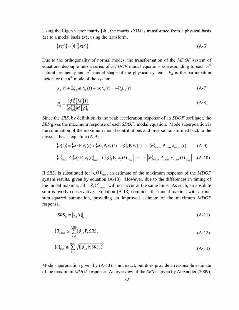
82
Using the Eigen vector matrix [Φ], the matrix EOM is transformed from a physical basis
{z} to a modal basis {x}, using the transform,
)()( txtz (A-6)
Due to the orthogonality of normal modes, the transformation of the MDOF system of
equations decouple into a series of n SDOF modal equations corresponding to each nth
natural frequency and nth
model shape of the physical system. Pn is the participation
factor for the nth
mode of the system.
)()()(2)( 2 tutxtxtx bninnnnn (A-7)
(A-8)
Since the SRS, by definition, is the peak acceleration response of an SDOF oscillator, the
SRS gives the maximum response of each SDOFn modal equation. Mode superposition is
the summation of the maximum modal contributions and inverse transformed back to the
physical basis, equation (A-9).
)()()()()( maxmaxmax333222111 txtxtxtxtu nnn (A-9)
maxmaxmaxmaxmax222max111max )()()( txtxtxu nnn
(A-10)
If SRSn is substituted for , an estimate of the maximum response of the MDOF
system results, given by equation (A-13). However, due to the differences in timing of
the modal maxima, all will not occur at the same time. As such, an absolute
sum is overly conservative. Equation (A-13) combines the modal maxima with a root-
sum-squared summation, providing an improved estimate of the maximum MDOF
response.
(A-11)
(A-12)
(A-13)
Mode superposition given by (A-13) is not exact, but does provide a reasonable estimate
of the maximum MDOF response. An overview of the SRS is given by Alexander (2009),
max
1
max
n
n
nnn SRSu
max
1
2
max
n
n
nnn SRSu
max)(txSRS nn
n
T
n
T
nn
M
MP
1
max)(txn
max)(txn
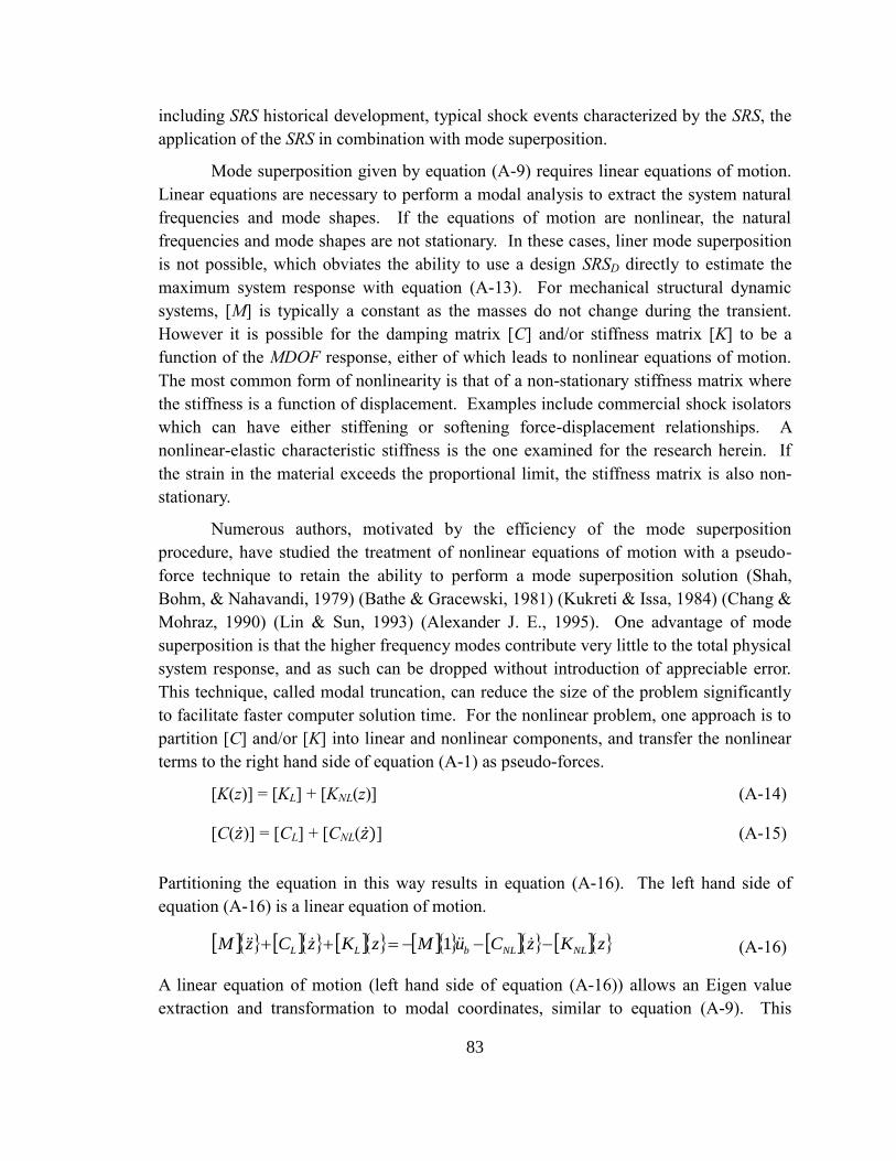
83
including SRS historical development, typical shock events characterized by the SRS, the
application of the SRS in combination with mode superposition.
Mode superposition given by equation (A-9) requires linear equations of motion.
Linear equations are necessary to perform a modal analysis to extract the system natural
frequencies and mode shapes. If the equations of motion are nonlinear, the natural
frequencies and mode shapes are not stationary. In these cases, liner mode superposition
is not possible, which obviates the ability to use a design SRSD directly to estimate the
maximum system response with equation (A-13). For mechanical structural dynamic
systems, [M] is typically a constant as the masses do not change during the transient.
However it is possible for the damping matrix [C] and/or stiffness matrix [K] to be a
function of the MDOF response, either of which leads to nonlinear equations of motion.
The most common form of nonlinearity is that of a non-stationary stiffness matrix where
the stiffness is a function of displacement. Examples include commercial shock isolators
which can have either stiffening or softening force-displacement relationships. A
nonlinear-elastic characteristic stiffness is the one examined for the research herein. If
the strain in the material exceeds the proportional limit, the stiffness matrix is also non-
stationary.
Numerous authors, motivated by the efficiency of the mode superposition
procedure, have studied the treatment of nonlinear equations of motion with a pseudo-
force technique to retain the ability to perform a mode superposition solution (Shah,
Bohm, & Nahavandi, 1979) (Bathe & Gracewski, 1981) (Kukreti & Issa, 1984) (Chang &
Mohraz, 1990) (Lin & Sun, 1993) (Alexander J. E., 1995). One advantage of mode
superposition is that the higher frequency modes contribute very little to the total physical
system response, and as such can be dropped without introduction of appreciable error.
This technique, called modal truncation, can reduce the size of the problem significantly
to facilitate faster computer solution time. For the nonlinear problem, one approach is to
partition [C] and/or [K] into linear and nonlinear components, and transfer the nonlinear
terms to the right hand side of equation (A-1) as pseudo-forces.
[K(z)] = [KL] + [KNL(z)] (A-14)
[C(�̇�)] = [CL] + [CNL(�̇�)] (A-15)
Partitioning the equation in this way results in equation (A-16). The left hand side of
equation (A-16) is a linear equation of motion.
(A-16)
A linear equation of motion (left hand side of equation (A-16)) allows an Eigen value
extraction and transformation to modal coordinates, similar to equation (A-9). This
zKzCuMzKzCzM NLNLbLL 1

84
procedure, however, still requires a transient analysis for updating [CNL] and [KNL] as the
system responses change.
Villaverde (1988) (1996) took another approach to nonlinear mode superposition.
The motivation was again that mode superposition is a quick, efficient procedure as
opposed to a time intensive nonlinear transient analysis with numerical integration.
Villaverde acknowledged that, while the approach gave approximate results, it had
adequate accuracy for preliminary design. Unlike the prior nonlinear mode superposition
approach described, Villaverde was able to avoid a transient analysis by development of a
nonlinear SRS, determined from a known transient design earthquake acceleration time-
history. The nonlinear SRS was determined from peak response values of nonlinear
SDOF oscillators. The nonlinearity of the oscillators examined was elastic-perfectly
plastic spring properties. Villaverde was one of the few authors who compared the results
of the approximate procedure with the exact transient results based on the response of
MDOF models. Comparison of Villarvede’s nonlinear SRS mode superposition
procedure approximate results to the exact result from the known earthquake acceleration
time-history transient analysis demonstrated average errors ranging from 8% to 40%
based on peak displacements for both 3DOF and 10DOF examples.
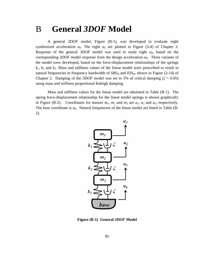
85
B General 3DOF Model
A general 3DOF model, Figure (B-1), was developed to evaluate eight
synthesized acceleration aS. The eight aS are plotted in Figure (3-4) of Chapter 3.
Response of the general 3DOF model was used to study eight aS, based on the
corresponding 3DOF model response from the design acceleration aD. Three variants of
the model were developed, based on the force-displacement relationships of the springs
k1, k2 and k3. Mass and stiffness values of the linear model were prescribed to result in
natural frequencies in frequency bandwidth of SRSD and EISD, shown in Figure (2-14) of
Chapter 2. Damping of the 3DOF model was set to 5% of critical damping (ζ = 0.05)
using mass and stiffness proportional Raleigh damping.
Mass and stiffness values for the linear model are tabulated in Table (B-1). The
spring force-displacement relationship for the linear model springs is shown graphically
in Figure (B-2). Coordinates for masses m1, m2 and m3 are u1, u2 and u3, respectively.
The base coordinate is ub. Natural frequencies of the linear model are listed in Table (B-
2).
Figure (B-1) General 3DOF Model
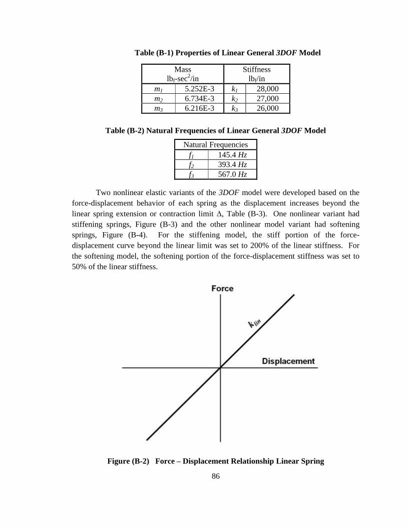
86
Table (B-1) Properties of Linear General 3DOF Model
Mass
lbf-sec2/in
Stiffness
lbf/in
m1 5.252E-3 k1 28,000
m2 6.734E-3 k2 27,000
m3 6.216E-3 k3 26,000
Table (B-2) Natural Frequencies of Linear General 3DOF Model
Natural Frequencies
f1 145.4 Hz
f2 393.4 Hz
f3 567.0 Hz
Two nonlinear elastic variants of the 3DOF model were developed based on the
force-displacement behavior of each spring as the displacement increases beyond the
linear spring extension or contraction limit Δ, Table (B-3). One nonlinear variant had
stiffening springs, Figure (B-3) and the other nonlinear model variant had softening
springs, Figure (B-4). For the stiffening model, the stiff portion of the force-
displacement curve beyond the linear limit was set to 200% of the linear stiffness. For
the softening model, the softening portion of the force-displacement stiffness was set to
50% of the linear stiffness.
Figure (B-2) Force – Displacement Relationship Linear Spring
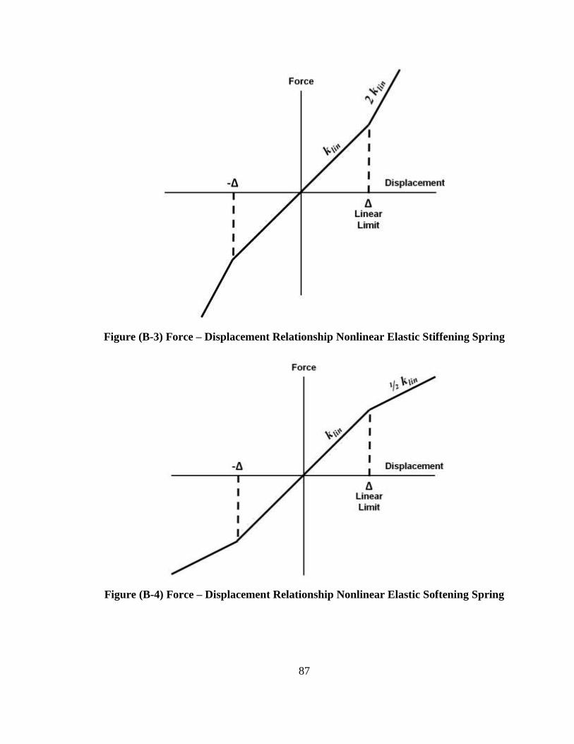
87
Figure (B-3) Force – Displacement Relationship Nonlinear Elastic Stiffening Spring
Figure (B-4) Force – Displacement Relationship Nonlinear Elastic Softening Spring
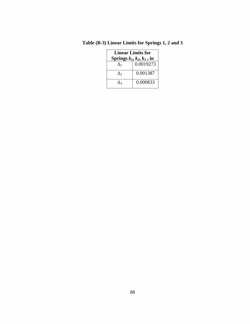
88
Table (B-3) Linear Limits for Springs 1, 2 and 3
Linear Limits for
Springs k1, k2, k3 , in
Δ1 0.0019273
Δ2 0.001387
Δ3 0.000833
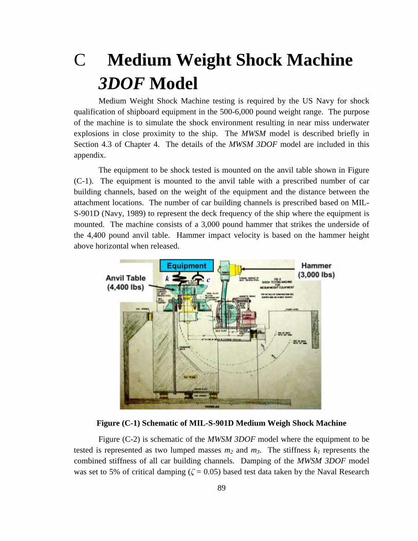
89
C Medium Weight Shock Machine
3DOF Model Medium Weight Shock Machine testing is required by the US Navy for shock
qualification of shipboard equipment in the 500-6,000 pound weight range. The purpose
of the machine is to simulate the shock environment resulting in near miss underwater
explosions in close proximity to the ship. The MWSM model is described briefly in
Section 4.3 of Chapter 4. The details of the MWSM 3DOF model are included in this
appendix.
The equipment to be shock tested is mounted on the anvil table shown in Figure
(C-1). The equipment is mounted to the anvil table with a prescribed number of car
building channels, based on the weight of the equipment and the distance between the
attachment locations. The number of car building channels is prescribed based on MIL-
S-901D (Navy, 1989) to represent the deck frequency of the ship where the equipment is
mounted. The machine consists of a 3,000 pound hammer that strikes the underside of
the 4,400 pound anvil table. Hammer impact velocity is based on the hammer height
above horizontal when released.
Figure (C-1) Schematic of MIL-S-901D Medium Weigh Shock Machine
Figure (C-2) is schematic of the MWSM 3DOF model where the equipment to be
tested is represented as two lumped masses m2 and m3. The stiffness k1 represents the
combined stiffness of all car building channels. Damping of the MWSM 3DOF model
was set to 5% of critical damping (ζ = 0.05) based test data taken by the Naval Research
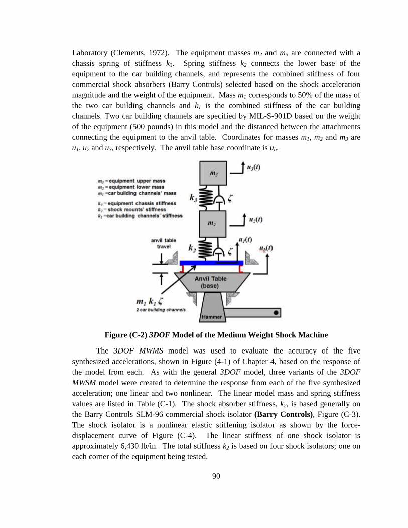
90
Laboratory (Clements, 1972). The equipment masses m2 and m3 are connected with a
chassis spring of stiffness k3. Spring stiffness k2 connects the lower base of the
equipment to the car building channels, and represents the combined stiffness of four
commercial shock absorbers (Barry Controls) selected based on the shock acceleration
magnitude and the weight of the equipment. Mass m1 corresponds to 50% of the mass of
the two car building channels and k1 is the combined stiffness of the car building
channels. Two car building channels are specified by MIL-S-901D based on the weight
of the equipment (500 pounds) in this model and the distanced between the attachments
connecting the equipment to the anvil table. Coordinates for masses m1, m2 and m3 are
u1, u2 and u3, respectively. The anvil table base coordinate is ub.
Figure (C-2) 3DOF Model of the Medium Weight Shock Machine
The 3DOF MWMS model was used to evaluate the accuracy of the five
synthesized accelerations, shown in Figure (4-1) of Chapter 4, based on the response of
the model from each. As with the general 3DOF model, three variants of the 3DOF
MWSM model were created to determine the response from each of the five synthesized
acceleration; one linear and two nonlinear. The linear model mass and spring stiffness
values are listed in Table (C-1). The shock absorber stiffness, k2, is based generally on
the Barry Controls SLM-96 commercial shock isolator (Barry Controls), Figure (C-3).
The shock isolator is a nonlinear elastic stiffening isolator as shown by the force-
displacement curve of Figure (C-4). The linear stiffness of one shock isolator is
approximately 6,430 lb/in. The total stiffness k2 is based on four shock isolators; one on
each corner of the equipment being tested.
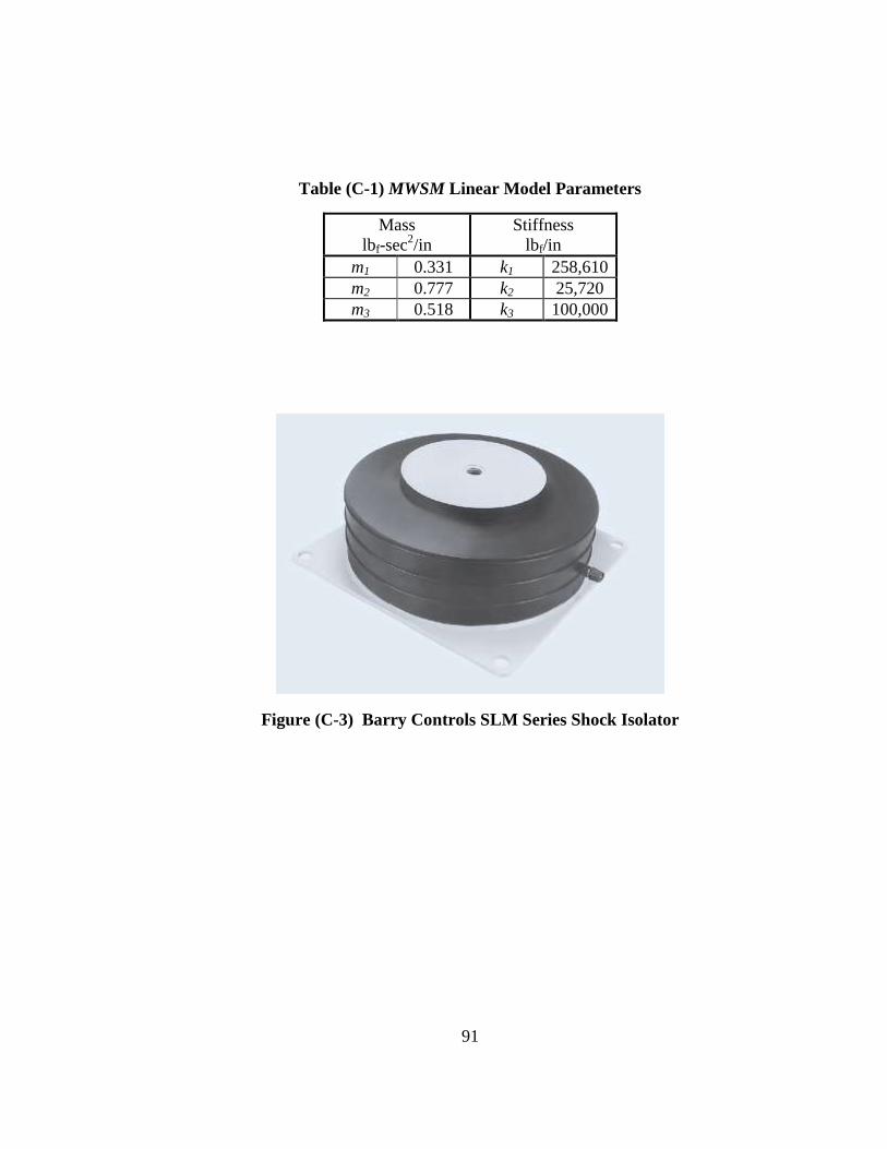
91
Table (C-1) MWSM Linear Model Parameters
Mass
lbf-sec2/in
Stiffness
lbf/in
m1 0.331 k1 258,610
m2 0.777 k2 25,720
m3 0.518 k3 100,000
Figure (C-3) Barry Controls SLM Series Shock Isolator
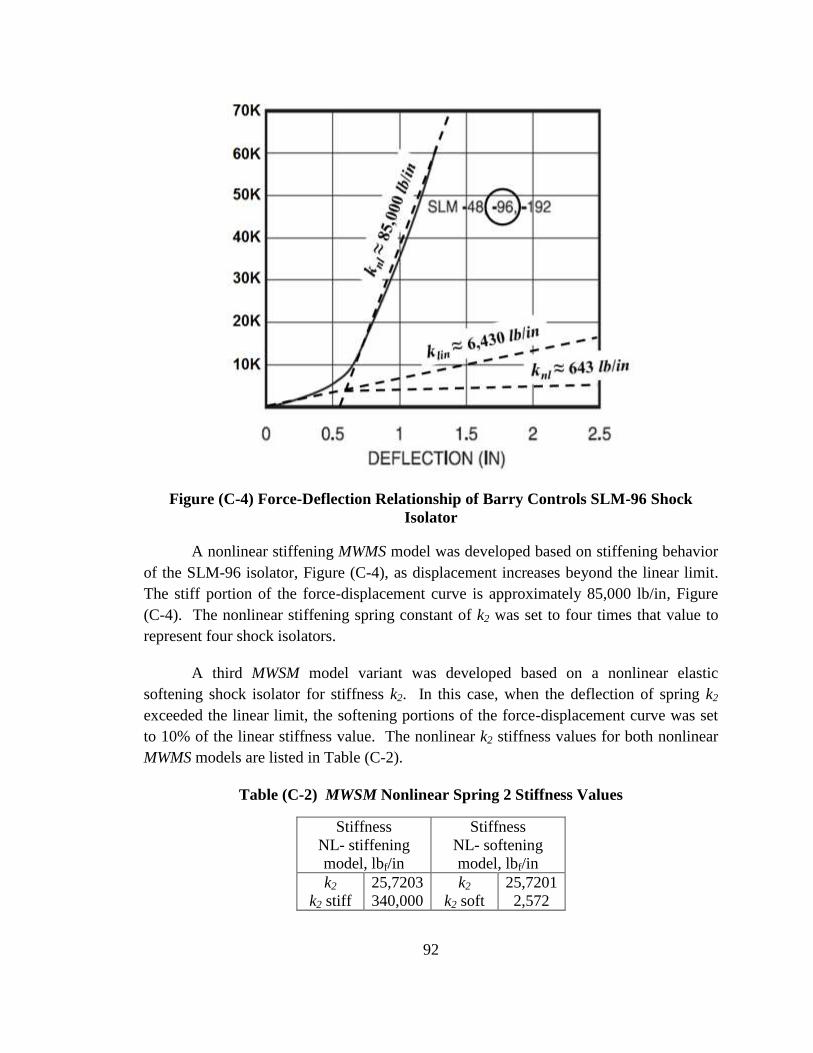
92
Figure (C-4) Force-Deflection Relationship of Barry Controls SLM-96 Shock
Isolator
A nonlinear stiffening MWMS model was developed based on stiffening behavior
of the SLM-96 isolator, Figure (C-4), as displacement increases beyond the linear limit.
The stiff portion of the force-displacement curve is approximately 85,000 lb/in, Figure
(C-4). The nonlinear stiffening spring constant of k2 was set to four times that value to
represent four shock isolators.
A third MWSM model variant was developed based on a nonlinear elastic
softening shock isolator for stiffness k2. In this case, when the deflection of spring k2
exceeded the linear limit, the softening portions of the force-displacement curve was set
to 10% of the linear stiffness value. The nonlinear k2 stiffness values for both nonlinear
MWMS models are listed in Table (C-2).
Table (C-2) MWSM Nonlinear Spring 2 Stiffness Values
Stiffness
NL- stiffening
model, lbf/in
Stiffness
NL- softening
model, lbf/in
k2
k2 stiff
25,7203
340,000
k2
k2 soft
25,7201
2,572
93
D Regression Analysis A summary of the regression analysis is discussed in Section 3.5 of Chapter 3.
Additional details of the regression analysis are in this appendix. The response of the
three variants of the general 3DOF model, described in Appendix B, is the basis for each
regression analysis. Nine individual regression analyses were performed to determine the
significance of the factors SRS%, EIS% and TE%. These analyses include three variants of
the general 3DOF model. An individual regression analysis includes the six factors and
one of the models responses of Table (D-1). For the nine total model responses of Tables
(D-1), (D-2) and (D-3) nine individual regression analyses were performed. The three
general 3DOF model variants were:
linear
nonlinear-stiffening
nonlinear-softening
Three responses used as the basis for the regression analysis for each model were:
average peak mass acceleration % error
average peak displacement % error
peak energy input % error
For each individual regression analysis, the general 3DOF model was subjected to the
eight synthesized accelerations listed in Table (3-1), and also plotted in Figure (3-4) of
Chapter 3. The factors evaluated were the percentage errors of the SRS, EIS and TE , from
each synthesized acceleration relative to the corresponding values from the design
acceleration aD. The regression analysis results for each variant of the general 3DOF
model are described individually in the following sections.
Significant factors for the general 3DOF models are indicated in Tables (D-1)
through (D-3). A significant factor for a model response is indicated by an “x” in the cell
corresponding to the factor and model response. The significance of the product of the
factors, or cross-terms, was also evaluated by the regression analysis.
The criteria for significance of a factor was set to an alpha value of less than or
equal to 0.10 (α ≤ 0.10). Alpha is frequently referred to as the level of significance.
Alpha is defined as the maximum level of risk for rejecting a true null hypothesis and is
expresses as a probability ranging between 0 and 1.
The regression analysis calculates a p-value for each factor. The p-value
represents the probability of incorrectly rejecting the null hypothesis. If the p-value is
less than or equal to the defined alpha value (α ≤ 0.10 in this case), the null hypothesis
(H0) can be rejected in favor of the alternative hypothesis (H1) (Minitab, Inc., 2014). In
94
this case, the null hypothesis H0 is that a factor is not statistically significant for a
response of the 3DOF model and the alternative hypothesis H1 is that the factor is
statistically significant for the response of the model.
R2 values are listed for each regression equation. R
2 indicates how well the model
(regression equation) fits the data. It is a value between 0 and 100%. Specifically, the R2
values indicated herein are “adjusted R2” which will increase only if a new term improves
the model more than would be expected by chance. Without adjustment, R2 will always
increase when a new term is added. Without this adjustment, a model with more terms
may appear to be a better fit even when it could be due to chance.
D1 General 3DOF Model – Linear
The regression model determined the significance of individual factors for each of
the three responses evaluated for the linear version of the general 3DOF model. Table
(D-1) indicates the significant factors for the linear variant of the general 3DOF model.
It is noted that individual factors can be significant, but also that the product of the
factors can also be significant.
Table (D-1) General 3DOF Model, Linear – Significant Factors
Model
Response
Factors
SRS% EIS% TE% (SRS%)(EIS%) (SRS%)(TE%) (EIS%)(TE%)
(peak mass
acceleration
% err)ave x x x
(peak
displacement
% err)ave x x x x
peak energy
input % err x x x
The regression model determines a predictive equation for each model response,
given by equations (D-1) through (D-3) for the linear 3DOF model.
(D-1)
(D-2)
(D-3)
%%%%
%%%
%
max
081.0023.0
805.0250.092.396.20
E
E
ave
TSRSEISSRS
TEISSRSz
%%%
%%
%
max
0504.0488.0
0211.0455.1716.9
EISSRST
EISSRSu
E
ave
))((152.0
11.2919.005.1014.7
%%
%%%
%
max
EISSRS
TEISSRSEn E
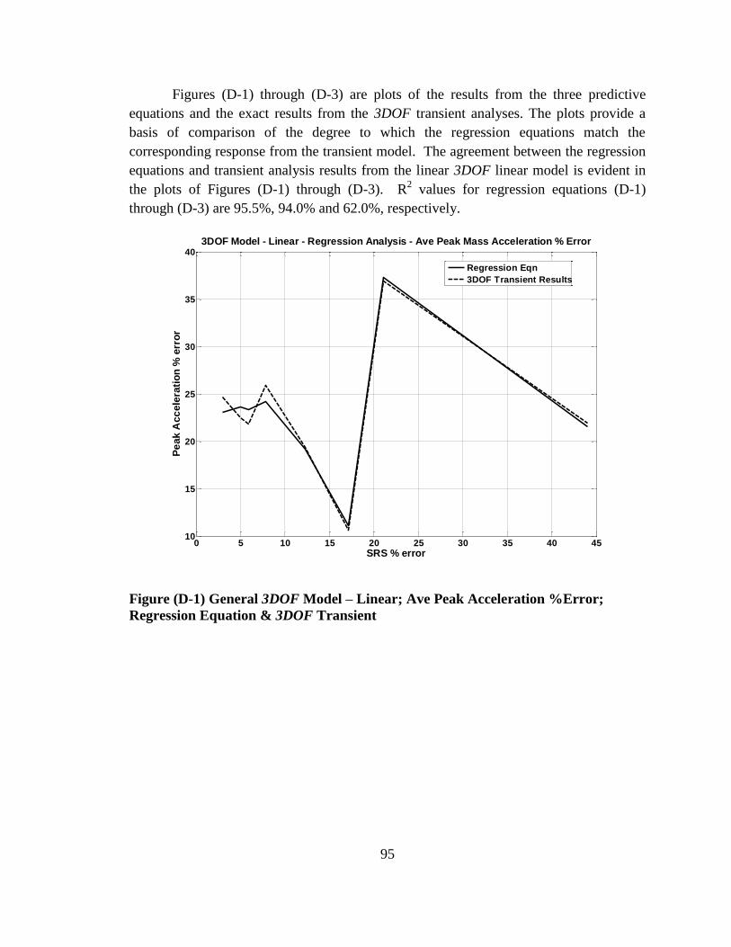
95
Figures (D-1) through (D-3) are plots of the results from the three predictive
equations and the exact results from the 3DOF transient analyses. The plots provide a
basis of comparison of the degree to which the regression equations match the
corresponding response from the transient model. The agreement between the regression
equations and transient analysis results from the linear 3DOF linear model is evident in
the plots of Figures (D-1) through (D-3). R2 values for regression equations (D-1)
through (D-3) are 95.5%, 94.0% and 62.0%, respectively.
Figure (D-1) General 3DOF Model – Linear; Ave Peak Acceleration %Error;
Regression Equation & 3DOF Transient
0 5 10 15 20 25 30 35 40 4510
15
20
25
30
35
403DOF Model - Linear - Regression Analysis - Ave Peak Mass Acceleration % Error
SRS % error
Pe
ak
Acc
ele
rati
on
% e
rro
r
Regression Eqn
3DOF Transient Results
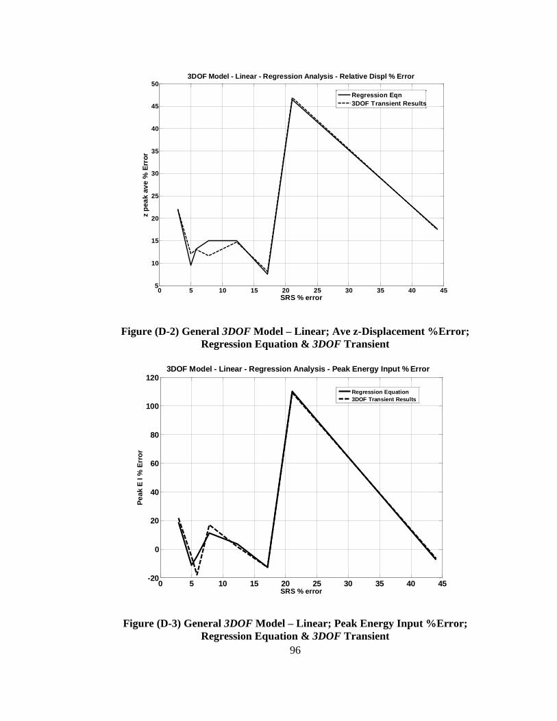
96
Figure (D-2) General 3DOF Model – Linear; Ave z-Displacement %Error;
Regression Equation & 3DOF Transient
Figure (D-3) General 3DOF Model – Linear; Peak Energy Input %Error;
Regression Equation & 3DOF Transient
0 5 10 15 20 25 30 35 40 455
10
15
20
25
30
35
40
45
503DOF Model - Linear - Regression Analysis - Relative Displ % Error
SRS % error
z p
ea
k a
ve %
Err
or
Regression Eqn
3DOF Transient Results
0 5 10 15 20 25 30 35 40 45-20
0
20
40
60
80
100
1203DOF Model - Linear - Regression Analysis - Peak Energy Input % Error
SRS % error
Pe
ak
E I %
Err
or
Regression Equation
3DOF Transient Results
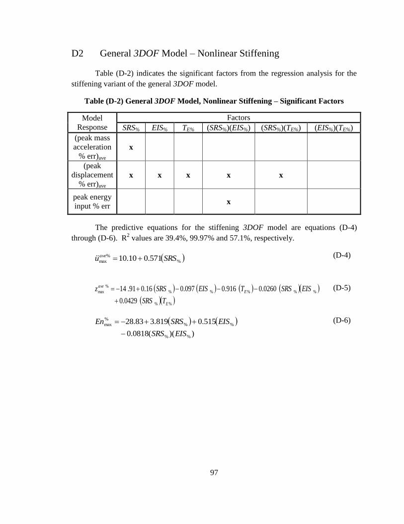
97
D2 General 3DOF Model – Nonlinear Stiffening
Table (D-2) indicates the significant factors from the regression analysis for the
stiffening variant of the general 3DOF model.
Table (D-2) General 3DOF Model, Nonlinear Stiffening – Significant Factors
Model
Response
Factors
SRS% EIS% TE% (SRS%)(EIS%) (SRS%)(TE%) (EIS%)(TE%)
(peak mass
acceleration
% err)ave x
(peak
displacement
% err)ave x x x x x
peak energy
input % err x
The predictive equations for the stiffening 3DOF model are equations (D-4)
through (D-6). R2 values are 39.4%, 99.97% and 57.1%, respectively.
(D-4)
(D-5)
(D-6)
%
%
max 571.010.10 SRSuave
%%
%%%%%
%
max
0429.0
0260.0916.0097.016.091.14
E
E
ave
TSRS
EISSRSTEISSRSz
))((0818.0
515.0819.383.28
%%
%%
%
max
EISSRS
EISSRSEn
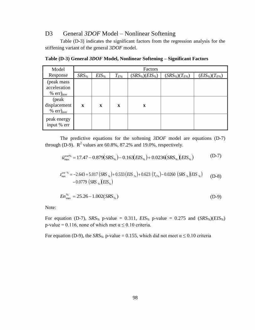
98
D3 General 3DOF Model – Nonlinear Softening
Table (D-3) indicates the significant factors from the regression analysis for the
stiffening variant of the general 3DOF model.
Table (D-3) General 3DOF Model, Nonlinear Softening – Significant Factors
Model
Response
Factors
SRS% EIS% TE% (SRS%)(EIS%) (SRS%)(TE%) (EIS%)(TE%)
(peak mass
acceleration
% err)ave
(peak
displacement
% err)ave x x x x
peak energy
input % err
The predictive equations for the softening 3DOF model are equations (D-7)
through (D-9). R2 values are 60.8%, 87.2% and 19.0%, respectively.
(D-7)
(D-8)
(D-9)
Note:
For equation (D-7), SRS% p-value = 0.311, EIS% p-value = 0.275 and (SRS%)(EIS%)
p-value = 0.116, none of which met α ≤ 0.10 criteria.
For equation (D-9), the SRS% p-value = 0.155, which did not meet α ≤ 0.10 criteria
%%
%%%%%
%
max
0779.0
0260.0623.0533.0017.5643.2
EISSRS
EISSRSTEISSRSz E
ave
)(002.126.25 %
%
max SRSEn
%%%%
%
max 0236.0163.0879.047.17 EISSRSEISSRSuave