A new derivation of Jeffery’s equation

Michael Junk∗ Reinhard Illner, †

Abstract

In this article, we present a modern derivation of Jeffery’s equationfor the motion of a small rigid body immersed in a Navier-Stokes flow,using methods of asymptotic analysis. While Jeffery’s result represents theleading order equations of a singularly perturbed flow problem involvingellipsoidal bodies, our formulation is for bodies of general shape and wealso derive the equations of the next relevant order.

Keywords. Jeffery’s equation, small immersed rigid body, asymptotic analysisAMS subject classifications.

1 Introduction

The original work of Jeffery [9], contains a derivation of approximate equationsof motion for a rigid ellipsoidal body immersed in a surrounding linear flowfield. While few details are given about the simplifying assumptions underlyingthe derivation, the main focus is put on a technical integral representation ofStokes solutions around general ellipsoids.Jeffery’s equations are widely used in the theory of suspensions where one triesto discover how the motion of a suspended particle and the suspending liquidinfluence each other. The single particle dynamics is then a basic ingredientfor statistical approaches which model the behavior of (dilute) ensembles ofsuspended particles. An extension of Jeffery’s work to more general geometriescan be found, for example, in [1] and [2] (for additional results on the topic,we refer to the review article [14].) An important application of the theory isthe description of injection molding of fiber reinforced plastics [15]. Moreover,the approach parallels in several respects the Leslie-Ericksen theory of rigid-rod liquid-crystalline polymers in the nematic phase [3, 11] and is also used inconnection with electrorheological fluids [6].In view of the importance of Jeffery’s equation, we think it is worth whilerevisiting the derivation. In contrast to Jeffery’s approach we are going tostress the basic assumptions in the derivation and try to keep our considerationslargely independent of the particular ellipsoidal geometry. Our argument isbased on an asymptotic expansion in ε (the size of the body) of the fluid velocity

∗FB Mathematik und Statistik, Fach D194, Universitat Konstanz, 78457 Konstanz, Ger-many,(michael.junk@uni-konstanz.de).

†Department of Mathematics and Statistics, University of Victoria, P.O. Box 3045, Victo-ria, B.C. V8W 3P4, Canada, (rillner@math.uvic.ca).

1

and pressure fields u, p as well as the center of mass coordinates and the angularvelocity c,ω of the rigid body (see figure 1) which satisfy a system of differentialequations.

PSfrag replacements

Ω

p

0

ωu

c

Figure 1: A small rigid body immersed in a flowing liquid.

It turns out that the leading order velocity field u0 is the undisturbed flow (i.e.without the rigid body) and that the center of mass of the body, also in leadingorder, follows the streamlines

c0(t) = u0(t, c0(t)). (1)

In the case of an elongated, rotationally symmetric ellipsoid, the orientationvector p in direction of the major semi-axis (see figure 1) obeys Jeffery’s equa-tion

p0 =1

2(curl u0) ∧ p0 + λ(S[u0]p0 − (pT

0 S[u0]p0)p0) (2)

up to an error of order ε, Here S[u0] is the symmetric part of the velocityJacobian, ∧ denotes the cross product, and the parameter

λ =(l/d)2 − 1

(l/d)2 + 1

is a function of the ratio l/d between the length of the long and the shortsemi-axis of the ellipsoidal body.Equation (2) appears as solvability condition of a Stokes problem which de-scribes the first order local flow around the small body (an explicit form of whichis derived in Jeffery’s article for the case of the ellipsoid). Such Stokes problemsare generally known as mobility problems and have been carefully studied (see,for example, [10]). In our approach, we extend these results by deriving also theequations for the second order coefficients and we show quantitatively how wellthe approximate solution obtained from the truncated asymptotic expansionsatisfies the coupled system of Navier-Stokes and rigid body equations. Thelatter result is a first step towards a mathematical proof that Jeffery’s equationis the correct asymptotic description of the ellipsoid dynamics.Our derivation of (2) is organized as follows. In section 2, we introduce the rel-evant equations which describe the moving particle. A non-dimensionalizationleads to an ε-dependent system of differential equations where ε is the ratioof body size versus the typical size of the flow domain. In section 3, we mo-tivate our ansatz for the asymptotic expansion and present the result for thetwo leading orders (details of the computation are given in appendix B). Thesolvability condition for the equations defining the expansion coefficients then

2

give rise to ordinary differential equations for the rotation state of the body andthe first order perturbation of the center of mass. The geometrical informationabout the body enters through weighted surface averages of six solutions of theStokes equation in the exterior domain. For general geometries, these valuescan be calculated using, for example, a boundary element method. However,in the special case of ellipsoidal geometries, the exact values are known, lead-ing to Jeffery’s equation if the ellipsoid has rotational symmetry (see section 4for details). Finally, in section 5, some particular solutions of Jeffery’s equa-tion are presented to illustrate the approximate motion of ellipsoidal bodies insurrounding flows.

2 Equations of motion

Our aim is to describe the motion of a small rigid body εE in a flowing liquid.We assume that the body template E ⊂ R

3 is an open and bounded domainwith a smooth surface ∂E, constant density ρb and center of mass at the origin,i.e.

∫

E

y dy = 0. (3)

Our main example will be the rotationally symmetric ellipsoid

E =

y ∈ R3 :

y21

l2+

y22 + y2

3

d2< 1

, l, d > 0 (4)

whose orientation in space can be described by a vector p which points in thedirection of the rotation axis. The forces which drive the rigid body originatein fluid friction and pressure acting on its surface. Since the body is moving, wefind a Navier-Stokes problem with moving boundary for the flow variables. Todescribe location and velocity of this boundary, we first consider the kinematicsof the rigid body. In the next step, we formulate the flow equations and, finally,we specify the rigid body dynamics.

2.1 Rigid body kinematics

The motion of a rigid body consists of translations and rotations. In particular,the position and orientation of the rigid body Eε(t) at time t is completelycharacterized by its center of mass c(t) ∈ R

3 and a rotation matrix R(t) ∈ SO(3)

Eε(t) = εR(t)E + c(t), t ≥ 0.

If we trace a body point y ∈ E, it follows the path x(t) = εR(t)y + c(t). Itsvelocity consists of the linear velocity c(t) and the angular velocity εR(t)y tobe investigated further. Writing R(t) as

R(t) =

(

limh→0

R(t + h)RT (t) − I

h

)

R(t), (5)

we are led to the rotation matrix R(t + h)RT (t) which is, for small h, a slightperturbation of the identity I. Its derivative at h = 0 is a so called infinites-

imal rotation (an element of the tangent space to SO(3) at the point I). An

3

elementary calculation (see for example [4, 5] or appendix A) shows that theinfinitesimal rotations in R

3 are the skew symmetric matrices which can bewritten as

B(ω) =

0 −ω3 ω2

ω3 0 −ω1

−ω2 ω1 0

, ω ∈ R3. (6)

We remark that B(ω)x is exactly the vector product between ω and x whichwe denote with ∧, i.e.

B(ω)x = ω ∧ x, ω,x ∈ R3. (7)

Relation (5) can now be cast into the form

R(t) = B(ω(t))R(t) (8)

with a suitable vector ω(t) ∈ R3 called angular velocity. In section 2.3, we will

describe the dynamics of the rigid body by specifying equations for c and ω.Note that the rotation matrix R(t) controlling the position of the rigid bodymay be recovered from ω by solving (8) with some initial value R(0).Coming back to the velocity of a body point x(t) = εR(t)y + c(t), we find

εR(t)y = εB(ω(t))R(t)y = B(ω(t))(x(t) − c(t))

leading to the velocity equation

x(t) = ω(t) ∧ (x(t) − c(t)) + c(t). (9)

From (9) we infer the evolution equation for an orientation vector p(t) pointingfrom the center of mass c(t) to some body point x(t)

p(t) = ω(t) ∧ p(t). (10)

In case of the ellipsoid (4) we will later focus on the orientation vector e1 whichpoints along the major semi-axis.

2.2 The flow problem

We assume that both the liquid and the rigid body Eε(t) are contained in aregular domain Ω ⊂ R

3. The liquid should be incompressible with constantdensity ρf and kinematic viscosity ν. Its pressure p and velocity field u satisfythe Navier-Stokes equation in Ω\Eε(t)

divu = 0, ∂tu + u · ∇u + ∇p/ρf = ν∆u (11)

complemented by suitable initial and boundary values. Without specifyingdetails, we assume that the boundary values on ∂Ω are chosen in such a waythat the undisturbed flow problem (no immersed body) is well posed. If arigid body Eε(t) = εR(t)E + c(t) is present in Ω, the no-slip condition on itsboundary implies in view of (9)

u(t,x) = ω(t) ∧ (x − c(t)) + c(t), x ∈ ∂Eε(t). (12)

4

To non-dimensionalize the equations, we choose a length scale L and a velocityscale U which are typical for the undisturbed flow. The corresponding time scaleis τ = L/U . As scale for viscous stress and pressure, we select Σ = ρfνU/L.Then, the scaled functions u(t, x) = u(τ t, Lx)/U and p(t, x) = p(τ t, Lx)/Σsatisfy

divxu = 0, Re(∂tu + u · ∇xu) = divxσ

where Re is the Reynolds number and σ the stress tensor

Re =UL

ν, σ = −pI + 2S[u], S[u] = (∇xu + ∇xuT )/2.

On the rigid body surface, we find

u(t, x) = ω(t) ∧ (x − c(t)) +d

dtc(t), x ∈ Eε(t)

where c(t) = c(τ t)/L, ω(t) = τω(τ t), and

Eε(t) = εR(t)E + c(t), ε = ε/L, R(t) = R(τ t).

2.3 Rigid body dynamics

In section 2.1 we have derived the velocity field inside the rigid body as

u(t,x) = ω(t) ∧ (x − c(t)) + c(t), x ∈ Eε(t)

so that the total linear momentum is given by

∫

Eε(t)ρbu(t,x) dx = ρb|Eε(t)|c(t) = ρbε

3|E|c(t). (13)

Here we have used (3) and | · | to denote the volume of a set. According toNewton’s law, the rate of change of (13) balances the forces acting on thebody which, in the present case, originate from the fluid stress σ acting on theboundary

ρbε3|E|c(t) =

∫

∂Eε(t)σn dS. (14)

Here, n is the normal field pointing out of Eε(t). For the total angular momen-tum with respect to the center of mass, we find

L(t) =

∫

Eε(t)ρb(x − c(t)) ∧ (u(t,x) − c(t)) dx

= −ρb

∫

Eε(t)(x − c(t)) ∧

[

(x − c(t)) ∧ ω(t)]

dx.

Using relation (7) we can write the vector products with x − c in terms of theskew symmetric matrix B(x − c) which eventually leads to

L(t) = ρbε5

∫

E

−B2(R(t)y) dy ω(t).

5

Finally, with relations (53) and (55) from the appendix, we get

L(t) = ρbε5|E|T (t)ω(t)

where T (t) is the inertia tensor

T (t) = R(t)TRT (t), T =1

|E|

∫

E

|y|2I − y ⊗ y dy. (15)

The equation for angular momentum now implies that the rate of change of L

is balanced by the angular momentum generated from the fluid stress on thesurface

ρbε5|E|

d

dt(T (t)ω(t)) =

∫

∂Eε(t)(x − c(t)) ∧ σn(x) dS. (16)

Introducing the same scaling as in the previous section, we derive from (14)and (16)

ε%Re

(

d

dt

)2

c(t) =1

|E|

∫

∂E

σ(t, X(t,y, ε))R(t)n(y) dS

ε2%Red

dt

(

T (t)ω(t))

=1

|E|

∫

∂E

(R(t)y) ∧ σ(t, X(t,y, ε))R(t)n(y) dS

where n is the outer normal field on ∂E, T (t) = R(t)T RT (t) and

X(t,y, ε) = εR(t)y + c(t).

The factor % is the quotient of body and fluid density % = ρb/ρf .

2.4 Summary

The unknowns in our problem are the flow variables p,u and the rigid bodyparameters c, R. Since we continue to work with the scaled variables, the hatsuperscripts are dropped from now on. With the mapping

X(t,y, ε) = εR(t)y + c(t), y ∈ R3

we can write the set Eε(t) = X(t, E, ε) occupied by the rigid body at time tin terms of the template body E which has its center of mass at y = 0. Theinverse mapping

Y (t,x, ε) = RT (t)x − c(t)

ε, x ∈ R

3 (17)

yields the template coordinates y corresponding to a space point x.On Ωε(t) = int(Ω\Eε(t)), the variables u, p satisfy the Navier-Stokes equation

divu = 0, Re(∂tu + u · ∇u) = −∇p + ∆u (18)

with boundary conditions on ∂Ω, initial conditions, and

u(t,x) = ω(t) ∧ (x − c(t)) + c(t), x ∈ ∂Eε(t). (19)

6

Further, we have

ε%Re c(t) =1

|E|

∫

∂E

σ(t,X(t,y, ε))R(t)n(y) dS (20)

ε2%Red

dt(T (t)ω(t)) =

1

|E|R(t)

∫

∂E

y ∧ RT (t)σ(t,X(t,y, ε))R(t)n(y) dS (21)

andR(t) = B(ω(t))R(t) (22)

complemented with suitable initial conditions. Here σij = −pδij +2Sij [u] is thefluid stress tensor with Sij[u] = (∂xj

ui + ∂xiuj)/2 and T (t) is the inertia tensor

T (t) = R(t)TRT (t), T =1

|E|

∫

E

|y|2I − y ⊗ y dy. (23)

We remark that (21) and (22) constitute a non-linear, second order differentialequation for R because ω can easily be calculated from (22) as

ω1 = (RRT )32, ω2 = (RRT )13, ω3 = (RRT )21.

Nevertheless, we keep ω as variable to simplify notation and because of thephysical relevance.

3 Asymptotic expansion

3.1 Basic assumptions

In order to obtain Jeffery’s equations (1), (2) as leading order dynamics ofthe rigid body evolution described in section 2.4, two basic assumptions aremandatory.

1) The flowing liquid is essentially undisturbed by the particle.

This assumption is reasonable if, for ε → 0, the mass of the small body andthus its momentum transfer to the fluid is negligible (which is the case for% = ρb/ρf = O(1)).

2) The fluid motion induces a rotation of the rigid body with angular velocityω = O(1).

From figure 2 we see that the velocity roughly varies between u0 − εω ∧ p

and u0 + εω ∧ p along a distance of order ε. Consequently, the local velocityfield around the particle (i.e. the difference to the undisturbed flow u0) has agradient of order one while its magnitude is of order ε. In contrast to this, thelocal pressure has to be of order one. Otherwise it cannot balance the viscousforces which are proportional to the symmetric part of the gradient of u.

7

PSfrag replacements

p

ε

u0

−εω ∧ p

Figure 2: Two dimensional projection of the rigid body Eε(t) moving essentiallywith the undisturbed velocity u0 plus an O(ε) disturbance due to an angularvelocity ω of order one. The gradient of the local velocity field is of order one.

To describe the local velocity and pressure field, it is convenient to work in thefixed body coordinates y. If εu1(t,y) is such a local velocity field (thoughtof as a perturbation from free flow u0), the actual velocity (perturbation) inx coordinates is εR(t)u1(t,Y (t,x, ε)), where Y is given by (17). Assumingthat u1 = O(1), we have exactly the situation that εu1 is of order ε but thex-gradient is of order one since ∇xY = O(ε−1). Similarly, the leading orderlocal pressure field is assumed of the form p1(t,Y (t,x, ε)). Altogether, we usethe following ansatz for the local fields

uloc(t,x) = εR(t)u1(t,Y (t,x, ε)) + ε2R(t)u2(t,Y (t,x, ε)) + . . . ,

ploc(t,x) = p1(t,Y (t,x, ε)) + εp2(t,Y (t,x, ε)) + . . . .(24)

If we assume polynomial decay rates for the local fields it turns out that theparticle has a small global influence. For example, if |u1(t,y)| ≈ C1|y|

−1 +C2|y|

−2 + . . . for large |y|, we have

|εR(t)u1(t,Y (t,x, ε))| ≈ ε2C1|x − c(t)|−1 + ε3C2|x − c(t)|−2 + . . .

Assuming that the particle stays away from the boundary, we see that the farfield of the local velocity influences the velocity distribution at ∂Ω in differentε orders starting at order ε2. Since we are aiming at most at second orderaccuracy, we can thus neglect higher order global fields (which ought to beincluded in a more accurate treatment). Thus, we end up with expansions ofthe form

u(t,x) = u0(t,x) + εR(t)u1(t,Y (t,x, ε)) + ε2R(t)u2(t,Y (t,x, ε)) + . . . ,

p(t,x) = p0(t,x) + p1(t,Y (t,x, ε)) + εp2(t,Y (t,x, ε)) + . . . ,

c(t) = c0(t) + εc1(t) + ε2c2(t) + . . . ,

ω(t) = ω0(t) + εω1(t) + . . . ,

R(t) = R0(t) + εR1(t) + . . . .

To obtain reasonable equations for the coefficients ui, pi, ci,ωi and Ri, theansatz is inserted into the equations listed in section 2.4, Taylor expansions arecarried out for ε → 0, and the appearing expressions in different orders of ε areequated to zero separately. For reasons of clarity, we will skip this step but useits result to define the expansion coefficients. In appendix B, we show that thecorresponding truncated expansion satisfies the original problem at least up toorder O(ε) which supports its validity.

8

Finally, we want to stress that our expansion of the flow variables is only rea-sonable as long as the rigid body stays away from the boundary ∂Ω becausewe assume the functions ui, pi to be defined in the unbounded exterior of thebody template E. Once the distance to the boundary is of the order of ε, thisassumption does not include the relevant physical effects.

3.2 Expansion coefficients

Here, we present the result of the asymptotic analysis outlined in the previoussection. We define the coefficients of the flow fields and the rigid body variablesaccording to the equations following from the expansion. The validity of theequations is checked, a posteriori, in appendix B.The leading order coefficients u0, p0 are defined as solutions of the incompress-ible Navier-Stokes problem in Ω

Re(∂tu0 + u0 · ∇u0) + ∇p0 = ∆u0, divu0 = 0 (25)

with the same initial and boundary values as the full problem in Section 2.4.The body center of mass is, at leading order, determined by

c0(t) = u0(t, c0(t)), c0(0) = c(0). (26)

The higher order perturbations ui, pi, i = 1, 2 are determined as solutions ofstationary Stokes problems in the exterior of the body template E

∇pi = ∆ui, divui = 0, in Ec (27)

with sufficiently fast decay at infinity (O(|y|−1) for velocity and O(|y|−2) forpressure and velocity gradient). At the body surface, we find integral conditionson the fluid stresses σi = −piI + 2S[ui]

∫

∂E

σin dS = gi,

∫

∂E

y ∧ σin dS = Gi (28)

and a Dirichlet condition

ui = bi = RT

0 Xi + H i on ∂E. (29)

The functions bi, gi,Gi and H i = bi − RT

0 X i have been introduced to avoidconfusing details which cloud the basic structure of the problem. They generallydepend on lower order expansion coefficients and are given in detail below. TheXi are the coefficients in the expansion of X(t,y, ε) = εR(t)y + c(t), i.e.

X0 = c0, X1 = R0y + c1, X2 = R1y + c2, . . . (30)

Finally, the matrices R0, R1 satisfy the differential equations

R0 = B(ω0)R0, R0(0) = R(0),

R1 = B(ω0)R1 + B(ω1)R0, R1(0) = 0(31)

9

and the initial values for ci are

c1(0) = 0, c2(0) = 0. (32)

To write the functions bi, gi,Gi in a compact form we use the differential oper-ators Di which appear in the Taylor expansion of an expression f(X 0 + εX1 +ε2X2 + . . . ) with respect to ε. More precisely, Di are defined by formallyequating orders in

∞∑

i=0

εi(Dif)(X0) =

∞∑

k=0

1

k!

[

∞∑

i=1

εi(Xi · ∇)

]k

f(X0)

so that Di depends on X0, . . . ,X i. For our purpose, we need

D0 = 1, D1 = X1 · ∇, D2 = X2 · ∇ +1

2(X1 · ∇)2.

In the first Stokes problem, we have

g1 = 0, G1 = 0, b1 = RT

0 (X1 − D1u0). (33)

Here and in the following, the derivatives of u0 are evaluated at time t andposition c0(t). The second Stokes problem is specified by

b2 = RT

0 (X2 − D2u0 − R1u1), (34)

g2 = %|E|ReRT

0 c0 −

∫

∂E

RT

0 D1σ0R0n dS, (35)

G2 = −

∫

∂E

y ∧ (RT

0 D1σ0R0n) dS. (36)

3.3 Solvability conditions

At first glance, the Stokes problems for u1 and u2 seem to be overdeterminedbecause of the extra requirements (28) apart from the Dirichlet conditions (29).However, a closer inspection reveals that the Dirichlet conditions (29) are notfully determined because they depend on the time derivative of the rigid bodyvariables ci and Ri−1 through Xi. Moreover, the number of degrees of freedomhidden in ci and Ri−1 match exactly the number of integral conditions. Notethat the vector ci has three components and the time derivative of Ri−1 is,in view of (31), also determined by three free parameters. In fact, we cansummarize (31) as

Ri = B(ωi)R0 + Ki (37)

where the matrix Ki depends on lower order terms and on Ri itself so thatthe equation for Ri is completely known once the three components of ω i aredetermined.We now show that there is only one choice for the six quantities such that both(28) and (29) are satisfied. These relations for ci, Ri−1 can therefore be viewedas solvability conditions for the Stokes problem. The basis for the proof is the socalled Faxen’s law [7,10,13] which relates the Dirichlet values bi of velocity with

10

the averaged force integrals gi and Gi. Following [13], the idea is as follows:we first construct particular solutions w1, . . . ,w6 of the Stokes equation in Ec

without source term and with Dirichlet boundary conditions

wk = ek k = 1, 2, 3, wk = y ∧ ek k = 4, 5, 6, on ∂E

where e4 = e1, e5 = e2 and e6 = e3. The stress tensors corresponding to wk

are denoted σ[wk]. Then (28) implies

ek · gi =

∫

∂E

wk · σin dS, k = 1, 2, 3.

Using the Green’s formula for the Stokes equation (see appendix C), it followswith the boundary condition (29)

ek · gi =

∫

∂E

bi · σ[wk]n dS, k = 1, 2, 3. (38)

Similarly, we have

ek · Gi =

∫

∂E

(B(y)σin) · ek dS = −

∫

∂E

(σin) · (B(y)ek) dS, k = 4, 5, 6

where the skew symmetry of B has been used in the last equality. Since wk =B(y)ek on ∂E, we obtain again with the help of Green’s formula

ek · Gi = −

∫

∂E

bi · σ[wk]n dS k = 4, 5, 6. (39)

We now replace bi by the more detailed structure given in equation (29). First,we note that (30) implies in connection with (37)

Xi = Ri−1y + ci = B(ωi−1)R0y + Ki−1y + ci.

Observing that for any rotation matrix R and any vector ω we have relation(55), i.e. RT B(ω)R = B(RT ω), it follows

RT

0 X i = B(RT

0 ωi−1)y +RT

0 ci +RT

0Ki−1y = −B(y)RT

0 ωi−1 +RT

0 ci +RT

0 Ki−1y,

so that, using skew symmetry of B,

bi · (σ[wk]n) = (RT

0 ωi−1) · (y ∧ σ[wk]n) + (RT

0 ci) · (σ[wk]n)

+ (RT

0 Ki−1y + H i) · (σ[wk]n) (40)

Inserting (40) into (38) and (39) we obtain with the abbreviation

F k =

∫

∂E

σ[wk]n dS, Mk =

∫

∂E

y ∧ σ[wk]n dS (41)

the following equations

F k · (RT

0 ci) + Mk · (RT

0 ωi−1) = Aki, k = 1, . . . , 6 (42)

11

where all terms independent of ωi−1 and ci are collected in Aki

Aki = −

∫

∂E

(RT

0 Ki−1y + H i) · σ[wk]n dS +

ek · gi k = 1, 2, 3

−ek · Gi k = 4, 5, 6. (43)

From the system (42) we can derive six independent explicit equations for thesix unknowns ci and ωi−1 (i.e. ordinary differential equations for ci and Ri−1)because the vectors Lk =

(

F k

−Mk

)

are linearly independent. According to thedefinition of F k, Mk, the components of Lk are given by

(Lk)j =

∫

∂E

wj · (σ[wk]n) dS.

The proof of linear independence is given in appendix C, Lemma 8.Altogether, we end up with the following pattern to determine the expansioncoefficients: first, u0, p0, c0 are calculated from (25) and (26). Then, c1,ω0 areobtained using the solvability condition (42) and c1, R0 follow by integrating theresulting ordinary differential equations. In the next step, the Stokes problem(27) with Dirichlet conditions (29) is solved to obtain u1, p1. The same patternapplies to the evaluation of u2, p2, c2, R1.

4 Extracting Jeffery’s equation

The aim of this section is to show that the solvability conditions (42) for c1 andω0 give rise to Jeffery’s equation in the special case of ellipsoidal bodies.Let us therefore consider (42) for the case i = 1. Since g1 = G1 = 0, K0 = 0(see (37)) and H1 = b1 − RT

0 X1 = −RT

0 D1u0 (see (29) and (33)), we have

Ak1 =

∫

∂E

(RT

0 D1u0) · σ[wk]n dS.

By observing that D1 = X1 · ∇ = (R0y + c1) · ∇, we see that

RT

0 D1u0 = RT

0∇u0(R0y + c1)

where all u0 derivatives are evaluated at (t, c0(t)). Splitting the gradient of u0

into symmetric and skew symmetric part and observing (55) and (58), we find

RT

0 D1u0 = B(RT

0 curlu0/2)y + (RT

0 S[u0]R0)y + RT

0∇u0c1

and since B(α)β = BT (β)α,

Ak1 =

(

1

2RT

0 curlu0

)

·

∫

∂E

B(y)σ[wk]n dS + (RT

0∇u0c1) ·

∫

∂E

σ[wk]n dS

+

∫

∂E

(RT

0 S[u0]R0)y · σ[wk]n dS

12

With the definition (41) we can cast the solvability conditions (42) for i = 1 inthe form

F k · RT

0 (c1 −∇u0c1) + Mk · RT

0 (ω0 − curlu0/2)

= (RT

0 S[u0]R0) :

∫

∂E

y ⊗ σ[wk]n dS, k = 1, . . . , 6 (44)

where (α ⊗ β)ij = αiβj and A : B = AijBij. We observe that only zero andfirst order moments of the surface force σ[wk]n are required to evaluate thecoefficients of (44). Note that in this way, geometry information about the rigidbody which is coded in the Stokes fields w1, . . . ,w6, enters the equation for c1

and ω0. For general shapes of E, the moments can be calculated, for example,with a boundary element method. However, in the special case of ellipsoidal

bodies, an explicit representation of σ[wk]n is available. In the following, weconcentrate on this case.

4.1 The case of ellipsoidal bodies

Let B1 = z ∈ R3 : |z| < 1 denote the unit ball in R

3. A general axis parallelellipsoid is then given by

E = DB1, D = diag(d1, d2, d3), di > 0.

Note that y ∈ E if and only if z = D−1y ∈ B1, i.e. if

(

y1

d1

)2

+

(

y2

d2

)2

+

(

y3

d3

)2

< 1.

Clearly, the center of mass is at the origin and the volume is given by |E| =|B1|detD.Combining the result in [13] with the expression (78) in appendix D for thesurface element, we can express the surface force on the ellipsoid as

(σ[wk]n)(y) dS(y) = αk det D wk(Dz) dS(z), y = Dz ∈ ∂E (45)

where αk are non-zero constants. Using this relation, it is possible to evaluateall required surface moments and the unspecified constants αk drop out in theend because they appear on both sides of (44). The detailed computation ofthe moments is given in appendix D. Here, we only list the results.The surface moments on the right hand side of (44) are given by

∫

∂E

y ⊗ σ[wk]n dS =

0 k = 1, 2, 3,

αk|E|D2B(ek) k = 4, 5, 6.

and for F k and Mk, we find

F k =

3αk|E|ek k = 1, 2, 3,

0 k = 4, 5, 6Mk =

0 k = 1, 2, 3,

−αk|E|Tek k = 4, 5, 6

13

where T is the inertia tensor of E defined in (23)

T =

d22 + d2

3

d21 + d2

3

d21 + d2

2

.

Inserting these results into (44), the solvability conditions decouple

c1 = ∇u0c1,

−ek · TRT

0 (ω0 − curlu0/2) = RT

0 S[u0]R0 : D2B(ek), k = 1, 2, 3

where the u0 expressions are evaluated at (t, c0(t)). Since the c1 equation ishomogeneous, the zero initial condition (32) implies c1(t) = 0 for all t, i.e. thesolvability conditions take the form c1 = 0 and

−ek · TRT

0 (ω0 − curlu0/2) = RT

0 S[u0]R0 : D2B(ek), k = 1, 2, 3. (46)

To see the relation between the equations for ω0 and Jeffery’s equation, somefurther transformations are necessary. We recall that ω0 is required to set upthe differential equation

R0 = B(ω0)R0, R0(0) = R(0)

for the leading order rigid body rotation R0. This matrix differential equationcan equivalently be written as three vector differential equations for the columnsp0i = R0ei. Note that each of these vectors points in the directions of a principalaxis. In appendix D we show that the three orientation vectors satisfy thedifferential equations

p0i =1

2(curl u0) ∧ p0i +

∑

k,m

εikmλmp0k ⊗ p0kS[u0]p0i, i = 1, 2, 3 (47)

where the tensor εikm is defined in section A.1 and the parameters λm are givenby the ratios

λ1 =d22 − d2

3

d23 + d2

2

, λ2 =d23 − d2

1

d21 + d2

3

, λ3 =d21 − d2

2

d22 + d2

1

.

Equation (47) is supplemented by initial conditions p0i(0) = R(0)ei accordingto (31).In the particular case where the ellipsoid is a body of rotation (i.e. d1 = land d2 = d3 = d), the orientation vectors p02,p03 are not required to specifythe spatial orientation of the body. They only describe how much the bodyhas rotated around the axis p01. This is nicely reflected by the fact that theequation for p01 decouples from the other two equations in that case. To seethis, we note that

λ1 = 0, λ3 = −λ2 = λ =(l/d)2 − 1

(l/d)2 + 1,

14

and the equation for the orientation vector p01 has the form

p01 =1

2(curlu0) ∧ p01 + λ

3∑

k=2

p0k ⊗ p0kS[u0]p01.

Taking into account that

3∑

k=1

p0k ⊗ p0k = R0

(

3∑

k=1

ek ⊗ ek

)

RT

0 = R0IRT

0 = I,

we can write

3∑

k=2

p0k ⊗ p0kS[u0]p01 = S[u0]p01 − p01 ⊗ p01S[u0]p01

and hence

p01 =1

2(curlu0) ∧ p01 + λ(S[u0]p01 − p01 ⊗ p01S[u0]p01).

Since the cubic term p01 ⊗ p01S[u0]p01 can be rewritten as (pT

01S[u0]p01)p01,we obtain upon renaming p0 = p01

p0 =1

2(curlu0) ∧ p0 + λ(S[u0]p0 − (pT

0 S[u0]p0)p0).

This is exactly Jeffery’s equation (2) which thus turns out to be the leadingorder solvability condition in the case of an elongated, rotationally symmetricellipsoidal body.

5 Some solutions

In this section, we try to illuminate the behavior of Jeffery’s equation in thecase of several stationary linear flow fields u0(x) = Ax. For several classesof matrices, explicit solutions of Jeffery’s equation are known. We will notlist these formulas here (they can be found, for example, in [8, 9]), but try toillustrate typical solutions.Coming back to the linear flow field, we stress that u0 is a solution of the Navier-Stokes equation if and only if A2 is symmetric and tr(A) = 0 (the divergencecondition). In this case the pressure is given by p(x) = −xT A2x. In two spacedimensions the symmetry of A2 is a consequence of the trace condition becausethe off-diagonal entries of A2 are A21tr(A) and A12tr(A). For truly three-dimensional flows, however, the conditions are independent, as the followingexample shows

A =

0 0 10 0 00 1 0

, A2 =

0 1 00 0 00 0 0

.

15

Even though the linear flow field is not a solution of the Navier-Stokes equationif A2 is not symmetric, it still satisfies the Stokes equation (together with aconstant pressure). Looking back at the asymptotic expansion, it is clear thata similar derivation is possible if we start with Stokes instead of Navier-Stokesequation. In this case, the leading order flow field u0 is an undisturbed Stokessolution. In that sense, it may also be reasonable to consider flows with A2 6=(A2)T .To explain our geometrical representation of the Jeffery solutions, let us beginwith the simple case of a purely rotational flow

u0(x) = Ax, A =

0 −1 01 0 00 0 0

.

Here, the symmetric part S[u0] of the Jacobian vanishes and curlu0 = 2e3, sothat Jeffery’s equation reduces to

p0 = e3 ∧ p0, p0(0) = p ∈ S2.

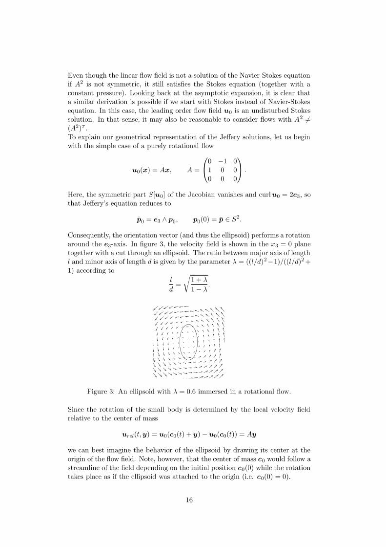
Consequently, the orientation vector (and thus the ellipsoid) performs a rotationaround the e3-axis. In figure 3, the velocity field is shown in the x3 = 0 planetogether with a cut through an ellipsoid. The ratio between major axis of lengthl and minor axis of length d is given by the parameter λ = ((l/d)2−1)/((l/d)2 +1) according to

l

d=

√

1 + λ

1 − λ.

Figure 3: An ellipsoid with λ = 0.6 immersed in a rotational flow.

Since the rotation of the small body is determined by the local velocity fieldrelative to the center of mass

urel(t,y) = u0(c0(t) + y) − u0(c0(t)) = Ay

we can best imagine the behavior of the ellipsoid by drawing its center at theorigin of the flow field. Note, however, that the center of mass c0 would follow astreamline of the field depending on the initial position c0(0) while the rotationtakes place as if the ellipsoid was attached to the origin (i.e. c0(0) = 0).

16

In order to show the dynamical behavior of the orientation vector, we can plot itspath on the unit sphere. In figure 4, the trajectories for several initial conditionsp0(0) = p are shown. In each case, the initial orientation is indicated by a littlepin. The markers along the curve are equidistant in time. As expected, thetrajectories are lines of equal latitude on the sphere because the rotation takesplace around the north-south axis.

Figure 4: Orientation trajectories in a rotational flow field (λ = 0.6).

The next example concerns a flow field which stretches e1 direction and com-presses in e2 direction

u0(x) = Ax, A =

1 0 00 −1 00 0 0

. (48)

Figure 5: An ellipsoid with λ = 0.8 immersed in a stretching flow. Left: flowfield in (x, y) plane. Right: flow field in (x, z) plane.

Since A is symmetric, there is no rotational part in Jeffery’s equation

p0 = λ(Ap0 − (pT

0 Ap0)p0), p0(0) = p ∈ S2. (49)

In order to find stationary solutions we consider the case of general symmetricflow matrices A. The condition for stationary states

Ap − (pT Ap)p = 0, p ∈ S2

17

implies that p is a normalized eigenvector of A with eigenvalue pT Ap. Inthe following, we denote the eigenvectors by p1,p2,p3 and the correspondingeigenvalues as µi.To check the stability of the stationary solutions, we calculate the derivative ofthe right hand side of (49) with respect to p. Observing that A =

∑

i µipi⊗pi,the derivative at p = pk turns out to be

3∑

i=1

(µi − µk − 2µkδik)pi ⊗ pi,

having the same eigenvectors as A. Obviously, the compressing directions (µk <0) are unstable, because the derivative at pk has a positive eigenvalue −2µk > 0.Conversely, if µk strictly dominates the other eigenvalues, the correspondingeigenvector is a stable state since µi − µk < 0 for all i. Another positiveeigenvalue µj belongs to an unstable state in that case because µk − µj > 0.The situation where two positive eigenvalues are of the same size is specialbecause there is no single direction associated to the stretching but a whole circle(the two-dimensional eigenspace intersected with the sphere). We consider thisexample later.In the case (48), we expect all generic trajectories to converge to the stretchingdirection e1 (see figure 6). Intuitively, this is also evident from the flow field(figure 5).

Figure 6: Trajectories of the orientation vector of an ellipsoid immersed in astretching flow converge to the stretching direction (λ = 0.8).

Next let us turn to the case

u0(x) = Ax, A =

1 0 00 1 00 0 −2

.

where the positive eigenvalues are of the same size. The flow field in the (x, y)plane is presented in figure 7 which suggests that every orientation vector issimply pulled into the (x, y)-plane. This can also be seen from the trajectories.

18

Figure 7: An ellipsoid with λ = 0.9 immersed in a stretching flow. Left: flowfield in (x, y) plane. Right: trajectories of the orientation vector.

The shear flow is a typical flow where rotation and stretching behavior is mixed.As example, we consider

u0(x) = Ax, A =

0 0 01 0 00 0 0

.

for which the flow field is presented in figure 8. The odd-even decomposition ofthe flow gradient A is

A =1

2

0 −1 01 0 00 0 0

+1

2

0 1 01 0 00 0 0

where the odd part describes a positively oriented rotation around the e3 axisand the even part is a stretching flow with eigenvalues −1, 1 and correspondingeigendirections (1, 1, 0)T and (−1, 1, 0)T .

Figure 8: An ellipsoid with λ = 0.99 immersed in a stretching flow. Left: flowfield in (x, y) plane. Right: flow field in (x, z) plane.

The corresponding Jeffery’s solutions are periodic (see [9, 14] for analytical so-lutions). In view of the flow field it is clear that the ellipsoid moves fastest, ifp is located in the (x, z) plane. But also in the orthogonal configuration, theshear flow leads to a rotation. Some trajectories are shown for different aspect

19

ratios l/d in figure 9. Note that for large aspect ratios, the orientation vectorspends most of its time close to the (y, z) plane which can be seen from themarker density along the trajectory. The reason is that the flow field alongthe sides of an ellipsoid pointing in y direction is very small. In the limit caseλ = 1, where the ellipsoid collapses to a line segment (d → 0), the y directionis a steady state.

Figure 9: Orientation behavior in shear flow. Left: λ = 0.7. Middle: λ = 0.95.Right: λ = 1.0.

We close our considerations with a flow that combines shearing and stretching(and which is only a Stokes solution since A2 6= (A2)T ).

u0(x) = Ax, A =

0.1 0 10 −0.1 00 0 0

.

In this flow, the orientation vector oscillates around and converges to the stableequilibrium (0, 1, 0).

Figure 10: An ellipsoid with λ = 0.7 immersed in a shearing and stretchingflow. Left: flow field in (x, y) plane. Right: orientation behavior.

A Rotations

Due to the non-linear structure of SO(3), the asymptotic expansion of an ε-dependent rotation matrix

R = R0 + εR1 + ε2R2 + ε3R3 + . . .

20

has the unpleasant property that any truncation at order m ≥ 1 generallyfails to be a rotation matrix. This leads to a few technicalities we want toaddress in section A.3. Apart from that, we prove some algebraic relationswhich are needed when manipulating skew symmetric matrices (section A.1).The relationship between rotations and skew symmetric matrices is highlightedin section A.2.

A.1 Skew symmetric matrices

The skew symmetric matrices in R3 can be parameterized in the basis ε1, ε2, ε3

ε1 = (ε1jk) =

0 0 00 0 +10 −1 0

, ε2 = (ε2jk) =

0 0 −10 0 0

+1 0 0

,

and

ε3 = (ε3jk) =

0 +1 0−1 0 00 0 0

.

Note that εijk = +1 if i, j, k is an even permutation of 1, 2, 3, εijk = −1 inthe case of an odd permutation, and εijk = 0 in the case that some indexappears twice. To abbreviate general linear combinations of the matrices εi, weintroduce

B(ω) =3∑

i=1

ωiεT

i =

0 −ω3 ω2

ω3 0 −ω1

−ω2 ω1 0

, ω ∈ R3. (50)

In the following, we employ Einstein’s summation convention which allows usto write the previous relation simply as B(ω)jk = ωiεikj. The results below aredirect consequences of definition (50).

Lemma 1 Let ω,x ∈ R3, R ∈ SO(3), and A ∈ R

3×3 be symmetric. Then

B(ω)x = ω ∧ x, (51)

B(ω)x = −B(x)ω, (52)

B(ω)2 = ω ⊗ ω − |ω|2I, (53)

B(ω)3 = −|ω|2B(ω), (54)

RB(ω)RT = B(Rω), (55)

tr(B(ω)A) = tr(AB(ω)) = 0. (56)

Proof: Relation (51) follows from the observation that (ω ∧ x)j = εjikωixk,and equation (52) is an immediate consequence of (51) and ω ∧ x = −x ∧ ω.To show (53), we note that εnjlεnki = δjkδli − δijδlk, and hence

B(ω)2ij = B(ω)inB(ω)nj = ωkωlεkniεljn = ωkωl(δjkδli − δijδlk)

= ωiωj − ωkωkδij = (ω ⊗ ω − |ω|2I)ij .

21

By multiplying (53) with B(ω) and noting that B(ω)ω = ω ∧ ω = 0, relation(54) follows. Due to the fact that RB(ω)RT in (55) is skew symmetric, thereexists some ω ∈ R

3 such that B(ω) = RB(ω)RT . Raising this equality to thethird power and using (54), we conclude |ω|2B(ω) = |ω|2B(ω). If we skip thetrivial case ω = 0, we can assume that both ω and ω are non-zero and theprevious relation allows us to conclude |ω| = |ω|. If we now square the relationB(ω) = RB(ω)RT and use (53), we obtain ω ⊗ ω = Rω ⊗ ωRT so that afterapplying a general vector x and scalar multiplying with Rω

(ω · x)(ω · Rω) = (ω · RT x)|ω|2, ∀x ∈ R3.

Thus, we conclude that

Rω =ω · Rω

|ω|2ω.

Taking norms on both sides and using the earlier result |ω| = |ω|, we see thatthe scalar factor (ω ·Rω)/|ω|2 can only be plus or minus one. Since ω dependsquadratically on R through the relation B(ω) = RB(ω)RT , the factor is a cubicpolynomial (and thus continuous) in the coefficients of R. Due to the fact thatSO(3) is connected and that the factor equals plus one for R = I ∈ SO(3), wehave proved ω = Rω. Finally, relation (56) follows from

tr(εiA) = εijkAjk = (εijk − εikj)Ajk/2 = (εijkAjk − εikjAkj)/2 = 0.

Note thattr(Aεi) = tr((Aεi)

T ) = −tr(εiA) = 0.

A.2 Rotations and skew symmetry

The following characterization shows that SO(3) is the image of the linear spaceof skew symmetric matrices under the exponential map.

Lemma 2 Let R ∈ SO(3). Then there exists ω ∈ R3 such that R = exp(B(ω))

Conversely, exp(B(ω)) ∈ SO(3) for all ω ∈ R3.

Proof: A simple argument shows that R has a normalized eigenvector a withcorresponding eigenvalue λ = 1. In fact, R has at least one real eigenvalue (asany 3 × 3 matrix), λ2 = (λa) · (λa) = (Ra) · (Ra) = |a|2 = 1, and detR = 1excludes the case that -1 can be an eigenvalue with odd multiplicity. Choosinga normalized vector e orthogonal to a, we define a rotation matrix M by speci-fying the columns (a , e , a∧ e). Then, using the skew symmetry of B(a), (53)and

R(a ∧ e) = RB(a)e = B(Ra)Re = a ∧ (Re),

we calculate

MT RM =

1 0 00 e · (Re) −(Re) · (a ∧ e)0 (Re) · (a ∧ e) e · (Re)

22

Since (Re) · a = (Re) · (Ra) = e · a = 0, we have

1 = |Re|2 = ((Re)·e)2+((Re)·a)2+((Re)·(a∧e))2 = ((Re)·e)2+((Re)·(a∧e))2

which implies the existence of ϕ ∈ [−π, π) with

(Re) · e = cos ϕ, (Re) · (a ∧ e) = sinϕ.

Using the relation(

cos ϕ − sinϕsinϕ cosϕ

)

= exp

(

0 −ϕϕ 0

)

we conclude M T RM = exp(B(ϕe1)), respectively

R = exp(MB(ϕe1)MT ) = exp(B(ϕMe1)) = exp(B(ω))

with ω = ϕa. The second statement follows from the observation

exp(B(ω)) exp(B(ω))T = exp(B(ω) + B(ω)T ) = exp(0) = I,

and from det exp(B(ω)) = exp(tr(B(ω))) = exp(0) = 1.

A similar characterization for smooth families of rotation matrices is the fol-lowing.

Lemma 3 Let R ∈ C1([0, tmax], SO(3)). Then there exists a function ω ∈C0([0, tmax], R3) such that

R(t) = B(ω(t))R(t), R(0) ∈ SO(3). (57)

Conversely, if ω ∈ C0([0, tmax], R3), then the solution of (57) gives rise to a

function R ∈ C1([0, tmax], SO(3)).

Proof: Define A(t) = R(t)RT (t). Taking the derivative of R(t)RT (t) = Ileads to A(t) + AT (t) = 0 with A ∈ C0([0, tmax], R3×3). Setting ω1 = A32,ω2 = A13, ω3 = A21, we have shown (57). Conversely, the unique solutionR ∈ C1([0, tmax], R3×3) of (57) satisfies R(t)RT (t) = I because the relationholds for t = 0 and the time derivative vanishes. The determinant D(t) ofR(t) follows the equation D(t) = tr(B(ω(t)))D(t) so that R(t) ∈ SO(3) sinceD(0) = 1.

In view of Lemma 2, the semigroup generated by a vector field w(x) = B(ω)x isthe family of rotations exp(tB(ω)). Similarly, the vector field w(x) = B(ω)x+v generates a rigid body motion consisting of a rotation and a translation.The following Lemma shows that these vector fields are characterized by theequation S[w] = 0 where S[w] = (∇w + (∇w)T )/2 is the symmetric part ofthe gradient ∇w. Note that the skew symmetric part (∇w − (∇w)T )/2 of ageneral vector field w can be written as B(α(x)) with

α =1

2

∂x2w3 − ∂x3

w2

∂x3w1 − ∂x1

w3

∂x1w2 − ∂x2

w1

=1

2curlw

23

so that

∇w =1

2B(curlw) + S[w]. (58)

Lemma 4 Let Ω ⊂ R3 be open and connected and assume w ∈ C2(Ω, R3)

satisfies S[w] = 0 in Ω. Then w(x) = B(ω)x + v for some ω,v ∈ R3.

Proof: Splitting the gradient of w in its symmetric and skew symmetricparts, we have ∇w = B(α(x)) for some function α ∈ C 1(Ω, R3). Since secondderivatives of the components wi commute, i.e.

∂2wi

∂xj∂xk

=∂2wi

∂xk∂xj, i, j, k = 1, 2, 3

we obtain nine conditions on the unknown function α. Due to the zero diagonalelements of B(α), we immediately find (see (50))

∂α3

∂x1=

∂α2

∂x1=

∂α3

∂x2=

∂α1

∂x2=

∂α2

∂x3=

∂α1

∂x3= 0.

The remaining three conditions are

−∂α3

∂x3=

∂α2

∂x2,

∂α3

∂x3= −

∂α1

∂x1, −

∂α2

∂x2=

∂α1

∂x1

from which we conclude that all components of α are constant, i.e. α(x) = ω

for some ω ∈ R3. Thus ∇w(x) = B(ω) which implies w(x) = B(ω)x + v for

some v ∈ R3.

A.3 Parameter dependent evolutions in SO(3)

Let M ε ∈ C1(R, SO(3)) : ε > 0 be a family of rotation matrix evolutionswith M ε(0) = R for all ε > 0. According to Lemma 3, M ε gives rise to somefunction ωε such that

M ε(t) = B(ωε(t))M ε(t), M ε(0) = R. (59)

If M ε,ωε have expansions of the form

M ε = R0 + εR1 + ε2R2 + . . . , ωε = ω0 + εω1 + ε2ω2 + . . .

the coefficients are related by

Ri =

i∑

k=0

B(ωk)Ri−k, R0(0) = R, Ri(0) = 0, i ≥ 1 (60)

which follows from inserting the expansions into (59) and matching orders in ε.Note that R0(t) is again a rotation matrix since R0 = B(ω0)R0, R0(0) = R but

24

this is not true for the higher order coefficients. For example, the first orderperturbation R1 satisfies

d

dt(RT

0 R1) = RT

0 B(ω0)T R1 + RT

0 (B(ω0)R1 + B(ω1)R0)

= RT

0 B(ω1)R0 = B(RT

0 ω1), (RT

0 R1)(0) = 0.

Hence

(RT

0 R1)(t) =

∫ t

0B(RT

0 (s)ω1(s)) ds

is a skew symmetric matrix so that R1 cannot be contained in SO(3). But eventhough the truncated expansion

Rε = R0 + εR1 + ε2R2 + · · · + εnRn

fails to be an element of SO(3), it is nevertheless close to the rotation matrixM ε. We exploit this relation to obtain the following result.

Lemma 5 Let ω0, . . . ,ωn ∈ C0([0, tmax], R3) with n ≥ 1 and define R0, . . . , Rn

as solutions of (60). Then there exists ε > 0 and c > 0 such that, for 0 < ε ≤ ε,

Rε = R0 + εR1 + ε2R2 + · · · + εnRn

is invertible, ‖(Rε)−1‖ ≤ c, and

‖(Rε)−1 − (Rε)T‖ ≤ cεn+1, ‖Rε − B(ωε)Rε‖ ≤ cεn+1

where ωε = ω0 + εω1 + · · · + εnωn and ‖ · ‖ is the sup-norm on [0, tmax].

Proof: Since the solutions R0, . . . , Rn of (60) are bounded in norm by someconstant c1 > 0, we have for ε ≤ 1 that

‖RT

0 (εR1 + ε2R2 + · · · + εnRn)‖ ≤ nc21ε.

Choosing ε = min1, 1/(2c21n), we obtain invertibility of Rε because ‖RT

0 Rε −I‖ ≤ 1/2 for ε ≤ ε implies invertibility of RT

0 Rε. Using von Neumann series,we also find the bound

‖(RT

0 Rε)−1‖ ≤1

1 − 12

= 2

so that ‖(Rε)−1‖ ≤ 2c1. To show that the inverse of Rε is essentially given by(Rε)T , we first note that

Rε =n∑

i=0

εii∑

k=0

B(ωk)Ri−k = B(ωε)Rε −2n∑

i=n+1

εi∑

k=i−n

B(ωk)Ri−k

which also implies the estimate on Rε − B(ωε)Rε. Using the relation, we find

d

dt((Rε)T Rε − I) = −(Rε)T B(ωε)Rε + (Rε)T B(ωε)Rε

+ εn+1n−1∑

i=0

εi

n∑

k=i+1

(

RT

n+1+i−kB(ωk)Rε − (Rε)T B(ωk)Rn+1+i−k

)

25

and since ((Rε)T Rε)(0) = RT R = I, we have with a suitable constant c2

‖(Rε)T Rε − I‖ ≤ c2εn+1.

Consequently, ‖(Rε)T − (Rε)−1‖ = ‖((Rε)T Rε − I)(Rε)−1‖ ≤ 2c1c2εn+1.

B Validation of the asymptotic expansion

Assuming that we have calculated the expansion coefficients as solutions of theequations given in section 3.2. Then we can set up the truncated expansions

cε = c0 + εc1 + ε2c2, ωε = ω0 + εω1.

For Rε = R0 + εR1, we just showed in appendix A, Lemma 5 that the inverseexists if ε > 0 is sufficiently small. Based on Rε, cε we define Xε(t,y, ε) =εRε(t)y + cε(t) with expansion coefficients

X0(t) = c0(t), X1(t,y) = R0(t)y + c1(t), X2(t,y) = R1(t)y + c2(t), . . .

and inverse

Y ε(t,x, ε) =1

ε(Rε(t))−1(x − cε(t)).

Finally, velocity and pressure fields are assumed to be sufficiently smooth givingrise to the truncated expansions

uε(t,x) = u0(t,x) +

2∑

i=1

εiRε(t)ui(t,Yε(t,x, ε)), (61)

pε(t,x) = p0(t,x) +

2∑

i=1

εi−1pi(t,Yε(t,x, ε)). (62)

In the following steps, we calculate the order at which the truncated expansionssatisfy the equations of section 2.4.

The rotation matrix: O(ε2)

For convenience, all technicalities concerning rotation matrices have been col-lected in the appendix A. In particular, since Ri,ωi satisfy equations (31), wecan use Lemma 5 which shows that

Rε = B(ωε)Rε + O(ε2),

i.e. Rε is an approximate solution of (22). Moreover, Lemma 5 yields theimportant relations

(Rε)−1 = (Rε)T + O(ε2), ‖(Rε)−1‖ = O(1) (63)

which will be frequently used.

26

The divergence condition: exact

Taking the divergence of a field

v(t,x) = Rε(t)v(t,Y ε(t,x, ε)) (64)

we find with Einstein’s summation convention

divv =∂vi

∂xi

= Rεij

∂vj

∂yl

1

ε(Rε)−1

li =1

ε

∂vl

∂yl

=1

εdivv.

Since all fields in (61) are divergence free, we conclude divuε = 0.

The Dirichlet condition: O(ε3)

We evaluate (19) at x = Xε(t,y, ε). Replacing terms by their approximatecounterparts, we have on the right hand side

ωε ∧ (Xε − cε) + cε = εB(ωε)Rεy + cε = εRεy + cε + O(ε3) = Xε+ O(ε3).

Evaluating the left hand side of (19), we need to expand the expression

u0(·,Xε) = u0(·,X0 + εX1 + ε2X2).

With the operators Di defined in the previous section and the relation X 0 = c0,we simply have

u0(t,Xε(t,y, ε)) =

2∑

i=0

εi(Di(t,y)u0)(t, c0(t)) + O(ε3).

Hence

uε(·,Xε) = u0 +2∑

i=1

εi (Diu0 + Rεui) + O(ε3).

Inserting the expansion of Rε and multiplying by RT

0 , we have

RT

0 (uε − ωε ∧ (Xε − cε) − cε) = RT

0 (u0 − c0)

+ ε(u1 + RT

0 (D1u0 − X1)) + ε2(u2 + RT

0 (R1u1 + D2u0 − X2)) + O(ε3)

which is of order ε3 in view of (26) and (29) with bi given by (33) and (34).

The linear momentum equation: O(ε2)

In order to calculate the fluid stress σε corresponding to the fields uε, pε, wenote that the Jacobian matrix of a field v of the form (64) is

(∇v)ij =∂vi

∂xj

= Rεik

∂vk

∂yl

1

ε(Rε)−1

lj =1

ε(Rε∇v(Rε)−1)ij (65)

For 2S[v] = ∇v+(∇v)T we conclude with (63) that S[v] = ε−1RεS[v](Rε)−1 +O(ε) so that

σε = −pεI + 2S[uε] = σ0 +

2∑

i=1

εi−1Rεσi(Rε)−1 + O(ε2). (66)

27

Evaluating this relation at x = Xε(t,y, ε) we need to expand the σ0 term.With the Di notation, we obtain

σ0(t,Xε(t,y, ε)) = σ0(t, c0(t)) + ε(D1(t,y)σ0)(t, c0(t)) + O(ε2).

In connection with (66), this yields

(Rε)−1σε(·,Xε)Rε = (Rε)−1σ0Rε + σ1 + ε(σ2 + (Rε)−1D1σ0R

ε) + O(ε2).

Replacing (Rε)−1 by (Rε)T on the right hand side and inserting the expansionof Rε in the first order term, we finally obtain

(Rε)−1σε(·,Xε)Rε = (Rε)T σ0Rε + σ1 + ε(σ2 + RT

0 D1σ0R0) + O(ε2). (67)

Noting that∫

∂E

(Rε)T σ0Rεn dS = (Rε)T σ0R

ε

∫

∂E

n dS = 0

we find on the right hand side of (20) after multiplying with |E|(Rε)−1

∫

∂E

(Rε)−1σεRεn dS =

∫

∂E

σ1n dS + ε

∫

∂E

(σ2 + RT

0 D1σ0R0)n dS + O(ε2).

The left hand side of (20) multiplied with |E|(Rε)−1 = |E|(Rε)T +O(ε2) yields

ε%|E|Re(Rε)−1cε = ε%|E|ReRT

0 c0 + O(ε2)

so that, in view of (33) and (35), the linear momentum equation is satisfied upto terms of order ε2.

The angular momentum equation: O(ε2)

Proceeding exactly as in the previous case, we multiply (21) by |E|(Rε)−1 andinsert our approximate quantities. On the right hand side we find with (67)and (63)

∫

∂E

y ∧ (Rε)T σεRεn dS =

∫

∂E

y ∧ (Rε)T σ0Rεn dS

+

∫

∂E

y ∧ σ1n dS + ε

∫

∂E

y ∧ (σ2 + RT

0 D1σ0R0)n dS + O(ε2). (68)

Noting that the symmetric matrix A = (Rε)T σ0Rε is independent of the inte-

gration variable, that

ei · (y ∧ An) = ei · B(y)An = −B(y)ei · An

= B(ei)y · An = AB(ei)y · n = AB(ei) : y ⊗ n

and that, with the divergence theorem,∫

∂E

yknl dS =

∫

E

div(ykel) dy = |E|δkl,

28

we conclude∫

∂E

y ∧ An dS = |E|AB(ei) : I = |E|tr(AB(ei)).

Using (56) in Lemma 1, appendix A, we conclude that the first integral on theright of (68) vanishes. Since the left hand side of (21) is already of order ε2,we see that (21) is satisfied up to order ε2 if (33) and (36) hold.

The Navier Stokes equation: O(ε)

With the abbreviation uloc, ploc for the sums of local fields in (61), (62), we firstcharacterize the different terms which appear when inserting uε = u0 + uloc,pε = p0 + ploc into the non-linear Navier Stokes equation. Since u0, p0 satisfy(25), we find

Re(∂tuloc + uloc · ∇u0 + u0 · ∇uloc + uloc · ∇uloc) = −∇ploc + ∆uloc. (69)

As before, we evaluate this equation at x = X ε(t,y, ε) and multiply both sideswith (Rε)−1. Elementary calculations in connection with (63) show that

(Rε)−1∇ploc =

2∑

i=1

εi−2(Rε)−1((Rε)−1)T∇pi =

2∑

i=1

εi−2∇pi + O(ε),

(Rε)−1∆uloc =

2∑

i=1

εi−2 ∂2ui

∂yl∂yk

[

(Rε)−1((Rε)−1)T]

kl=

2∑

i=1

εi−2∆ui + O(ε)

where terms on the left are evaluated at (t,X ε(t,y, ε)) and on the right at(t,y). Using (27), we conclude

(Rε)−1(−∇ploc + ∆uloc) =2∑

i=1

εi−2(−∇pi + ∆ui) + O(ε) = O(ε). (70)

To evaluate the time derivative ∂tuloc, we first study a typical term (64). Wehave

∂tv(t,x) = Rε(t)v(t,Y ε(t,x, ε)) + Rε(t)(∂tv)(t,Y ε(t,x, ε))

+ Rε(t)(∇v)(t,Y ε(t,x, ε))Yε(t,x, ε).

Taking space and time derivatives of the relation Y ε(t,Xε(t,y, ε), ε) = y, weobtain

Yε(t,Xε(t,y, ε), ε) = −(∇Xε)−1(t,y, ε)X

ε(t,y, ε) = −

1

ε(Rε(t))−1X

ε(t,y, ε).

Thus,

(Rε)−1∂tuloc =2∑

i=1

εi(∂tui + (Rε)T Rεui) −2∑

i=1

εi−1∇ui(Rε)T X

ε+ O(ε2).

29

In view of (70), the truncation error on the right hand side of (69) is of orderO(ε). Truncating the time derivative at the same order, we have

(Rε)−1∂tuloc = −∇u1RT

0 X0 + O(ε). (71)

Finally, we consider the quadratic terms in (69). Writing directional derivatives(v · ∇)w as matrix vector products (∇w)v, and observing (65), we find

(Rε)−1(uloc · ∇u0 + u0 · ∇uloc + uloc · ∇uloc) =

2∑

i=1

εi(Rε)T∇u0Rεui

+2∑

i=1

εi−1∇ui(Rε)T u0 +

2∑

i,j=1

εi+j−1∇uiuj + O(ε2) (72)

where all expressions in ui are evaluated at (t,y) and those in u0,uloc at(t,Xε(t,y, ε)). The latter require additional expansion which introduces theoperators Dj. Note that only the second sum in (72) contains a zero order term∇u1R

T

0 D0u0 which can be combined with (71). Since D0u0 − X0 = u0 − c0,equation (26) implies that this zero order contribution vanishes. Thus, theNavier-Stokes equation is satisfied up to terms of order ε.

C The Green’s formula

The Green’s formula is based on the rule for the divergence of a product betweena stress tensor σ = −pI + 2S[w], where 2S[w]ij = ∂xi

wj + ∂xjwi, and a vector

field v. We have

div(σv) = (−∇p + ∆w) · v + 2S[w] : S[v] − pdivv + v · ∇divw, (73)

where A : B = AijBij . As a first consequence, we derive an integration by partsformula.

Lemma 6 Let E ⊂ R3 be a bounded domain with smooth boundary ∂E. As-

sume further that vi, qi,f i, i = 1, 2 are smooth functions on the closure of Ec

with decay property

|vi(x)| ≤c

|x|, |∇vi(x)|, |qi(x)| ≤

c

|x|2, |f i(x)| ≤

c

|x|3

for |x| ≥ R > 0. If vi, qi are solutions of the Stokes equations

divσi = f i, divvi = 0 in Ec

with (σi)kl = −qiδkl + ∂xk(ui)l + ∂xl

(ui)k, they satisfy the Green’s formula

∫

∂E

v1 · (σ2n) dS +

∫

Ec

v1 · f2 dx =

∫

∂E

v2 · (σ1n) dS +

∫

Ec

v2 · f1 dx (74)

where n is the outer normal field to E.

30

Proof: We present a proof for completeness. More details can be found in[12]. Let BR be a ball with radius R > R such that E ⊂ BR. The divergencetheorem implies

∫

Ec∩BR

div(σ2v1) dx = −

∫

∂E

(σ2v1) · n dS +

∫

∂BR

(σ2v1) · n dS.

Using (73), we find div(σ2v1) = 2S[v1] : S[v2] + v1 · f2, so that

∫

Ec∩BR

2S[v1] : S[v2] dx +

∫

Ec∩BR

v1 · f2 dx

= −

∫

∂E

v1 · (σ2n) dS +

∫

∂BR

(σ2v1) · ndS.

Note that symmetry of σ2 has been used in the first integral on the right.Subtracting the corresponding equation with reversed roles of indices and usingthe decay properties, (74) follows.

With a very similar proof, we obtain the following result.

Lemma 7 Let E ⊂ R3 be a bounded domain with smooth boundary ∂E. As-

sume further that v, q are smooth solutions of the Stokes equation

∇q = ∆v, divvi = 0 in Ec

with decay property

|v(x)| ≤c

|x|, |∇v(x)|, |q(x)| ≤

c

|x|2

for |x| ≥ R > 0. Then,

∫

∂E

v · (σn) dS = 2

∫

Ec

S[v] : S[v] dx (75)

where n is the outer normal field to E and σ = −qI + 2S[v].

Using Lemma 7 we can show the invertibility of the matrix

Lkj =

∫

∂E

wj · (σ[wk]n) dS, k, j = 1, . . . , 6 (76)

where w1, . . . ,w6 are of the Stokes equation in Ec without source term andwith Dirichlet boundary conditions

wk = ek k = 1, 2, 3, wk = y ∧ ek k = 4, 5, 6, on ∂E (77)

The vectors e4, e5, e6 as synonym for the standard unit vectors e1, e2, e3 in R3.

The stress tensors corresponding to wk are denoted σ[wk] = −qkI + 2S[wk]with pressure functions qk.

31

Lemma 8 Let E ⊂ R3 be a bounded domain with smooth boundary ∂E. As-

sume further that wk, qk, k = 1, . . . , 6 are smooth solutions of the homogeneous

Stokes equation with Dirichlet conditions (77) on the closure of E c with decay

property

|vk(x)| ≤c

|x|, |∇vk(x)|, |qk(x)| ≤

c

|x|2, |x| ≥ R > 0.

Then the matrix L ∈ R6×6 given in (76) is invertible.

Proof: Let us assume that λ ∈ R6 is in the kernel of L. In particular, we

have

0 =

6∑

j,k=1

λkLkjλj =

∫

∂E

w · (σ[w]n) dS, w =

6∑

k=1

λkwk.

According to Lemma 7, we conclude S[w] = 0 and Lemma 4 implies w(x) =B(α)x + v. Since all wk are decaying at infinity, it follows that α = v = 0 sothat w vanishes. In particular, w vanishes at the boundary ∂E and since theboundary values (77) are linearly independent, all λk must be zero which showsthe injectivity of L. Since L is a square matrix, invertibility follows.

D Details for the ellipsoidal geometry

D.1 The surface measure

We consider the ellipsoid

E = DB1, D =

d1

d2

d3

, d1 > 0.

where B1 = z ∈ R3 : |z| < 1 denotes the unit ball in R

3. The tangent spaceat y ∈ ∂E is spanned by Dt1, Dt2 where t1, t2 are tangential at z = D−1y. Inparticular,

0 = z · ti = (D−1y) · ti = (D−2y) · (Dti) i = 1, 2

so that n = D−2y/|D−2y| is the normal vector at y ∈ ∂E. To calculate thechange in surface volume when passing from ∂B1 integrals to ∂E integrals, weconsider the rectangle with sides t1 and t2 at z ∈ ∂B1. The image of thisrectangle has sides Dt1, Dt2 and its area is given by

det(Dt1 , Dt2 , n) =1

|D−2y|det(Dt1 , Dt2 , D−2y)

=detD

|D−2y|det(t1 , t2 , D−3y)

32

Projecting D−3y onto the normal D−1y at ∂B1, we have

det(Dt1 , Dt2 , n) =detD

|D−2y|(D−3y) · (D−1y) det(t1 , t2 , D−1y).

Since det(t1 , t2 , D−1y) is the area of the original rectangle, the volume changeis given by

dS(z) =dS(y)

detD|D−2y|, z = D−1y. (78)

D.2 Surface moments

Using expression (45) for the surface force on the ellipsoid

(σ[wk]n)(y) dS(y) = αk det D wk(Dz) dS(z), y = Dz ∈ ∂E

we now calculate the required moments in (44) which are for k = 1, . . . , 6

F k =

∫

∂E

σ[wk]n dS, Mk =

∫

∂E

y ∧ σ[wk]n dS, Sk =

∫

∂E

y ⊗ σ[wk]n dS.

In general, a P moment of the surface force is given by∫

∂E

P (y)(σ[wk]n)(y) dS(y) = αk detD

∫

∂B1

P (Dz)wk(Dz) dS(z).

If P is a homogeneous polynomial, then we can write the surface integral over∂B1 as volume integral over B1. In fact if Q is a homogeneous polynomial ofdegree l

∫

B1

Q(x) dx =

∫ 1

0

∫

∂B1

Q(rz) dS r2 dr

=

∫ 1

0rl+2 dr

∫

∂B1

Q(z) dS =1

l + 3

∫

∂B1

Q(z) dS

Thus, the resulting expression for the moments of the surface force is∫

∂E

P (y)σ[wk]n dS = αk|E|(l + 3)1

|B1|

∫

B1

P (Dx)wk(Dx) dx (79)

where the fields wk inside of the body are defined as continuation of theirpolynomial values on the boundary

wk(y) = ek k = 1, 2, 3, wk(y) = y ∧ ek k = 4, 5, 6, y ∈ E

and l is the degree of Pwk, i.e. l = deg P for k = 1, 2, 3 and l = 1 + deg P fork = 4, 5, 6.To compute the coefficients F k in (44), we choose P (y) = 1. Noting that,because of symmetry, polynomials of odd degree average to zero over the unitball, we immediately find

F k =

3αk|E|ek k = 1, 2, 3,

0 k = 4, 5, 6.

33

For M k and Sk, we choose P (y) ∈ y1, y2, y3. Again, the averages of odddegree polynomials vanish which now involves k = 1, 2, 3. On the other hand,the product of yi with wk(y) gives rise to general homogeneous second orderpolynomials (l = 2). We remark that

1

|B1|

∫

B1

(Dx) ⊗ (Dx) dx = D1

|B1|

∫

B1

x ⊗ x dxD =1

5D2. (80)

To calculate M 4,M 5,M 6, we take P (y) = B(y) in (79). Since wk(y) =B(y)ek, k = 4, 5, 6, we have P (y)wk(y) = B2(y)ek = (y ⊗ y − |y|2I)ek and,in view of (79) and (80)

Mk = αk|E|(D2 − (trD2)I)ek, k = 4, 5, 6.

Note that

D2 − (trD2)I =1

|B1|

∫

B1

(Dx) ⊗ (Dx) − |Dx|2I dx =1

|E|

∫

E

y ⊗ y − |y|2I dy

is, up to the sign, the inertia tensor T of E defined in (23)

T =

d22 + d2

3

d21 + d2

3

d21 + d2

2

.

Thus,

Mk =

0 k = 1, 2, 3,

−αk|E|Tek k = 4, 5, 6.

Since the degree of y ⊗ wk(y) is odd for k = 1, 2, 3, the moment matrix Sk

vanishes in that case. For k = 4, 5, 6, we have

y ⊗ B(y)ek = −y ⊗ B(ek)y = −y ⊗ yBT (ek) = y ⊗ yB(ek)

and with l = 2 in (79) and (80) we eventually get

Sk =

0 k = 1, 2, 3,∫

∂Ey ⊗ σ[wk]n dS = αk|E|D2B(ek) k = 4, 5, 6.

D.3 Evolution of orientation vectors

In section 4.1, we have seen that the leading order solvability conditions reduceto the equations (46)

−ek · TRT

0 (ω0 − curlu0/2) = RT

0 S[u0]R0 : D2B(ek), k = 1, 2, 3

if the body under consideration is an ellipsoid. Using this specification of ω0,we can set up the differential equation

R0 = B(ω0)R0, R0(0) = R(0) (81)

34

for the leading order rigid body rotation R0, or equivalently, for the threeorientation vectors p0i = R0ei.In order to derive these equations for p0i, we first calculate the right hand sideof (46) explicitly. Setting A = RT

0 S[u0]R0, we find

A : D2B(ek) =

(d23 − d2

2)A23

(d21 − d2

3)A13

(d22 − d2

1)A21

k

, k = 1, 2, 3

and by bringing the inertia tensor T to the right hand side, (46) reduces to

RT

0 (ω0 − curlu0/2) = Λ

A23

A13

A21

, Λ =

d2

2−d2

3

d2

3+d2

2

d2

3−d2

1

d2

1+d2

3

d2

1−d2

2

d2

2+d2

1

. (82)

Next, we combine this result with equation (81) for which we need B(ω0).Applying B to the left hand side of (82) and observing (55), we find

B(RT

0 (ω0 − curlu0/2)) = RT

0 B(ω0)R0 − RT

0 B(curlu0/2)R0.

Denote the diagonal entries of Λ in (82) by λi and setting a = (A23, A13, A21)T ,

we obtain with symmetry of A

B(Λa) =

0 −λ3A12 λ2A13

λ3A21 0 −λ1A23

−λ2A31 λ1A32 0

and the differential equation for R0 reads

R0 = B(ω0)R0 =1

2B(curlu0)R0 + R0B(Λa). (83)

The matrix equation can equivalently be written as a system of equations forthe columns p0i = R0ei. Considering, for example, the first column, we find

R0B(Λa)e1 = R0

0λ3

−λ2

Ae1 = R0(λ3e2 ⊗ e2 − λ2e3 ⊗ e3)Ae1.

Note that the tensor product terms are of the form ε1kmλmek ⊗ ek. Moreover,we have A = RT

0 S[u0]R0 and R0ek ⊗ ekRT

0 = (R0ek) ⊗ (R0ek) so that, ingeneral,

R0B(Λa)ei =∑

k,m

εikmλmp0k ⊗ p0kS[u0]p0i, i = 1, 2, 3.

Hence, by applying (83) to the vectors ei, we end up with the following systemof equations

p0i =1

2curlu0 ∧ p0i +

∑

k,m

εikmλmp0k ⊗ p0kS[u0]p0i, i = 1, 2, 3

which is supplemented by initial conditions p0i(0) = R(0)ei according to (81).

35

References

[1] H. Brenner. Rheology of a dilute suspension of axisymmetric Brownianparticles. Int. J. Multiphase flow, 1:195–341, 1974.

[2] F.P. Bretherton. The motion of rigid particles in a shear flow at lowReynolds number. J Fluid Mech., 14:284–304, 1962.

[3] M. Doi and S.F. Edwards. The theory of polymer dynamics. ClarendonPress, Oxford, 1987.

[4] W.H. Fleming. Functions of several variables. Springer, 1977.

[5] H. Goldstein. Classical mechanics. Addison-Wesley, 1990.

[6] T.C. Halsey, J.E. Martin, and D. Adolf. Rheology of electrorheologicalfluids. Phys. Rev. Letters, 68:1519–1522, 1992.

[7] J. Happel and H. Brenner. Low Reynolds number hydrodynamics, with

special applications to particulate media. Leyden: Noordhoff, 1973.

[8] E.J. Hinch and L.G. Leal. The effect of Brownian motion on the rheolog-ical properties of a suspension of non-spherical particles. J. Fluid. Mech.,52:683–712, 1972.

[9] G.B. Jeffery. The motion of ellipsoidal particles immersed in a viscousfluid. Proc. Roy. Soc. London A, 102:161–179, 1922.

[10] S. Kim and S.J. Karrila. Microhydrodynamics, Principles and selected

applications. Butterworth-Heinemann, 1991.

[11] N. Kuzuu and M. Doi. Constitutive equation for nematic liquid crystalsunder weak velocity gradient derived from a molecular kinetic equation. J.

Phys. Soc. Japan, 52:3486–3494, 1983.

[12] O.A. Ladyzhenskaya. The mathematical theory of viscous incompressible

flow. Gordon and Breach, 1963.

[13] N. Liron and E. Barta. Motion of a rigid particle in Stokes flow: anew second-kind boundary-integral equation formulation. J. Fluid. Mech.,238:579–598, 1992.

[14] C.J.S. Petrie. The rheology of fibre suspensions. J. Non-Newt. Fluid Mech.,87:369–402, 1999.

[15] C.L. Tucker III and S.G. Advani. Processing of short-fiber systems. In S.G.Advani, editor, Flow and Rheology in Polymer Composites Manufacturing,pages 147–202. Elsevier, Amsterdam, The Netherlands, 1994.

36