A derivation of the beam equation

Daniel DuqueCanal de Experiencias Hidrodinamicas (CEHINAV)

E.T.S. Ingenieros NavalesAvda. Arco de la Victoria 4, 28006 Madrid (Spain)

December 7, 2015

Abstract

The Euler-Bernoulli equation describing the deflection of a beam is avital tool in structural and mechanical engineering. However, its deriva-tion usually entails a number of intermediate steps that may confuse en-gineering or science students at the beginnig of their undergraduate stud-ies. We explain how this equation may be deduced, beginning with anapproximate expression for the energy, from which the forces and finallythe equation itself may be obtained. The description is begun at the levelof small “particles”, and the continuum level is taken later on. However,when a computational solution is sought, the description turns back tothe discrete level again. We first consider the easier case of a string un-der tension, and then focus on the beam. Numerical solutions for severalloads are obtained.

1 Motivation

The Euler-Bernoulli beam equation is of paramount importance in civil engi-neering, being a simplified theory that yields relevant results for the dynamicsand statics of beams [1, 2, 3]. From the mathematical point of view, it is per-haps the simplest differential equation of a high order (fourth) that has a clearpractical relevance. However, a simple derivation is not easy to find, since mostoften a number of intermediate concepts, such as bending moments and shearforces, are introduced. We have designed a seminar in which the beam equa-tion is obtained from an expression for the energy. As a preliminary step, theequation for the string under tension is derived, in a manner slightly differentfrom what is usual. Computational methods are employed for both systems, inorder to find numerical solutions.

This article explains the method used. Its contents would fit in about twohours, ideally followed by a practical computing session of about two hours.

1

arX

iv:1

512.

0117

1v1

[ph

ysic

s.ge

n-ph

] 3

Dec

201

5

2 Introduction

Depending on the level of the class, some introduction to elementary Newtonianparticle mechanics may be needed. In particular, Newton’s Second Law, and thecase when forces are conservative and can therefore be obtained as derivativesof some potential energy.

However, Newton’s laws deal with point particles and forces between them.They are very accurate at scales such as the Solar System, at which the planetsand the Sun are almost point-like. Another regime ln which Newtonian physicsworks very well is at very small scales, where molecules or atoms are againalmost point-like (even if the interactions themselves have a quantum origin).

Everyday objects, on the other hand, are usually extended (continuum). His-torically, “particles” have been introduced in order to apply point dynamics tothese systems. Particles are portions of material that are “very” small, yet still“large enough” to have macroscopic features, such as density, volume, temper-ature, etc. In practical terms, they can be as small as small cells, about 1 µmin size. If they are smaller, thermal effects can cause such effects as Brown-ian motion. Of course, the students should not relate these particles, with realparticles, such as electrons.

The idea behind this approach is to apply Newtonian physics to each ofthese particles. Then, one takes the continuum limit, in which the number ofthese particles, N , is taken to infinity, but some of their features are taken zero(others may stay tend to infinity or reach a finite value.) As a simple example,the mass of each particle, m could tend to zero in such a way that the totalmass, given by

M = Nm

remains constant. The same applies for lengths and other quantities, even if insome cases, as we will see, the correct limit is not obvious to anticipate.

This way, one may derive laws expressed as partial differential equations.For example, we will derive here the wave equation:

∂2y

∂t2= v2

∂2y

∂x2

and the beam equation:∂2y

∂t2= −EI ∂

4y

∂x4+ q

Traditionally, many special mathematical methods have been devised tosolve these equations, leading to huge advances in mathematics, physics, andengineering [4]. The advent of computing has changed the situation somewhat,often providing a more direct and easier way to find solutions (or more precisely,a numerical approximation to the solutions.) On the other hand computers arediscrete by nature. A continuum equation can therefore not be computed as is:it must be discretized. The conclusion, as we will discuss, is that we return towhere we started, two centuries ago [5].

2

3 The string

This is system covered in many textbooks, but we treat it here for two reasons.The first is that the procedure will be mirrored when discussing the beam, butthe expressions are simpler in this case. The second is that some of the quantitiesthat are introduced in elementary textbooks (chiefly, the tension) arise naturallyin this procedure.

We model a string as a line of point particles (we will call “beads”) joined bymassless springs. Of course, most strings are not built this way, but the pointis that the continuum limit will be the same for a wide number of systems, andwe choose a simple one to work with.

3.1 Energy

The expression for the energy of a spring comes from Hooke’s law:

U =1

2κ(`− `0)2,

where `0 is the spring’s natural length and `, its actual length. The elasticparameter κ is Hooke’s spring constant. This is the best known expression, buthere we will prefer to use an expression that features the relative deformation,(`− `0)/`0, called the “strain”:

U =1

2

B

`0(`− `0)2,

where B = κ`0 is a parameter with units of force, whose meaning will bediscussed later.

Let us first consider the string under tension, but unperturbed otherwise.Its shape will be a straight line as in the upper part of Figure 1, and all thespring lengths will be equal to d, with d > `0. The energy will therefore be

U0 = N × 1

2

B

`0(d− `0)2 =

1

2

B

`0N(dN − `0N)2 =

1

2

B

L0(L− L0)2.

In order to reach the later equality we have multiplied and divided by N , andwe have written Nd = L for the length of the string and N`0 = L0 for its naturallength. This is actually our first application of the continuum limit, since webegin with an expression that depends on the particles’ magnitudes d and `0and we end up with another one that depend on the macroscopic magnitudesL and L0. Also, the parameter B seems to require no change with N in orderthe energy U be finite. Since B = κ`0, the string constant κ should then tendto infinity (not to zero!) in this limit.

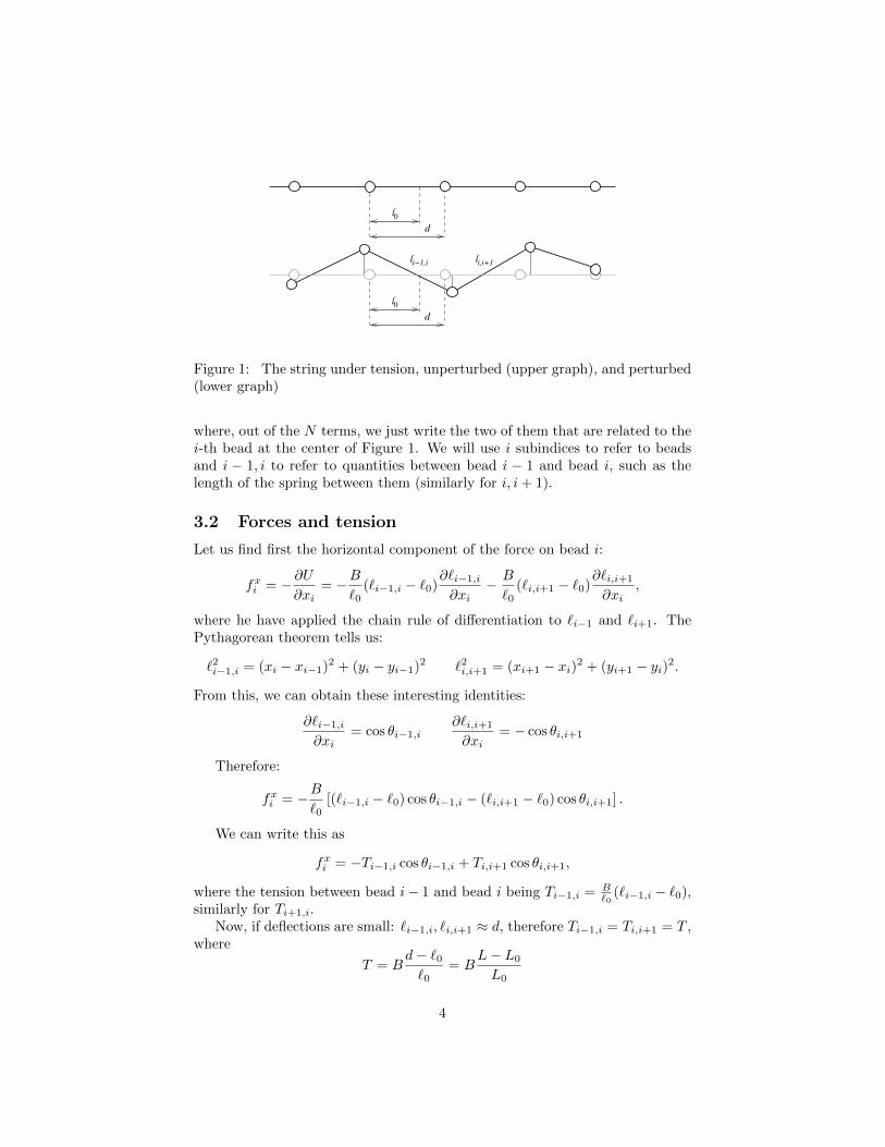
If, on the other hand, the string is distorted, as in the lower part of Figure1, the energy will now be:

U =1

2

B

`0(`i−1,i − `0)2 +

1

2

B

`0(`i,i+1 − `0)2 + · · · ,

3

l0

d

l0

li,i+1l

d

i−1,i

Figure 1: The string under tension, unperturbed (upper graph), and perturbed(lower graph)

where, out of the N terms, we just write the two of them that are related to thei-th bead at the center of Figure 1. We will use i subindices to refer to beadsand i − 1, i to refer to quantities between bead i − 1 and bead i, such as thelength of the spring between them (similarly for i, i+ 1).

3.2 Forces and tension

Let us find first the horizontal component of the force on bead i:

fxi = − ∂U∂xi

= −B`0

(`i−1,i − `0)∂`i−1,i∂xi

− B

`0(`i,i+1 − `0)

∂`i,i+1

∂xi,

where he have applied the chain rule of differentiation to `i−1 and `i+1. ThePythagorean theorem tells us:

`2i−1,i = (xi − xi−1)2 + (yi − yi−1)2 `2i,i+1 = (xi+1 − xi)2 + (yi+1 − yi)2.

From this, we can obtain these interesting identities:

∂`i−1,i∂xi

= cos θi−1,i∂`i,i+1

∂xi= − cos θi,i+1

Therefore:

fxi = −B`0

[(`i−1,i − `0) cos θi−1,i − (`i,i+1 − `0) cos θi,i+1] .

We can write this as

fxi = −Ti−1,i cos θi−1,i + Ti,i+1 cos θi,i+1,

where the tension between bead i− 1 and bead i being Ti−1,i = B`0

(`i−1,i − `0),similarly for Ti+1,i.

Now, if deflections are small: `i−1,i, `i,i+1 ≈ d, therefore Ti−1,i = Ti,i+1 = T ,where

T = Bd− `0`0

= BL− L0

L0

4

Moreover, cos θi,i+1 ≈ 1 for all beads, therefore fx ≈ 0.Notice this tension T is the external force to be applied to the ends of the

string to keep it tout. Indeed, the left end particle (i = 1) has no neighbor atits left to pull from it, and the tension T must be applied from the outside.The same applies to the other end. Moreover, recalling the total energy isU0 = 1

2BL0

(L− L0)2, we see T ′ = −dU/dL = −T . What this means is that thestring is trying to shrink with a force T ′ that we must overcome with anotherone T which is equal but pointing outwards.

The B parameter is then seen to be

B = TL0

L− L0=

T

(L− L0)/L0.

One of the important elastic properties of a material is its Young’s modulus(also known as tensile modulus, or elastic modulus), a magnitude with units ofpressure that is defined as the stress/strain ratio:

E =T/A0

(L− L0)/L0.

The strain is, as in Hooke’s law, (L − L0)/L0, and the stress is the tensiondivided by the cross section of the string under no tension, A0. Therefore, ourB parameter is related to Young’s modulus:

B = EA0.

As a simple experiment, students can try to measure experimentally values ofYoung’s modulus from these equations, see Appendix B.

The vertical component of the force follows from the identity

∂`i−1,i∂yi

= sin θi−1,i∂`i,i+1

∂yi= − sin θi,i+1,

with the end result:

fyi = −Ti−1,i sin θi−1,i + Ti,i+1 sin θi,i+1,

Many physics books, such as [6, 7, 8], basically start with this equation forthe vertical force, from considerations of the net vertical on each bead. Ourderivation has the advantage of providing more insight on the meaning of thetension T . It is also less likely to result in errors in signs. On the other hand,in [9] we find a derivation similar to ours (although it is given in terms of rodscoupled by torsion.)

In the limit of small vertical deflections, the force may be written as

fyi = −T sin θi−1,i + T sin θi,i+1

In this limit, the sines are also similar to the tangents, so:

fyi ≈ −T

d(yi − yi−1) +

T

d(yi+1 − yi) =

T

d(yi−1 − 2yi + yi+1)

5

3.3 The wave equation

Let us continue with the equations of motion for our bead. Newton’s SecondLaw gives (only the y direction is changing, so we will drop the y superindices):

mai =T

d(yi−1 − 2yi + yi+1)

that can be written as

ai =T

m/d

yi−1 − 2yi + yi+1

d2=T

µ

yi−1 − 2yi + yi+1

d2,

with µ = m/d the mass per unit length.The last ratio is a discrete, finite differences, version of the second spatial

derivative [10]. Therefore, in the limit d→ 0 we may write the wave equation

a =∂2y

∂t2=T

µ

∂2y

∂x2.

It can be shown that the phase velocity of traveling waves is given by v2 = T/µ.

3.4 The loaded string

It is often interesting to find the equilibrium solution to equations, setting thetime derivatives equal to zero. In this case, it is rather dull: the solution to∂2y∂x2 = 0 is just a straight line. For homogeneous Dirichlet boundary conditionsy(0) = y(L) = 0, the unique solution is simply y(x) = 0.

To make things more interesting, we may add a vertical force F (x) to eachbead. This force is constant in the vertical direction, but may vary along thestring. The energy equation would be modified as:

U = · · · − F (x)y.

The wave equation is now:

∂2y

∂t2=T

µ

∂2y

∂x2+ F/m

The static solution is given by the equation:

T

µ

∂2y

∂x2= −F/m

This is a Poisson equation. For example, for the case of gravity one wouldhave

F = −mg → T

µ

∂2y

∂x2= g.

Setting y(0) = y(L) = 0, the unique solution is a parabola:

y = −µg2T

x(L− x). (1)

6

Some students may know the solution to this sort of problems involvinghanging strings is often more involved, with shapes such as the catenary re-sulting. That is the case, but in this limit of small deformations the solutionis simply an upward parabola, which is the usual limit of any curve close to aminimum.

3.5 Computing the loaded string

A computer may be used in order to find the equilibrium shape of a string undergeneral loads. However, in order to apply computational methods we need togo back to the discretized equations, which are the ones that are readily imple-mented on a computer. This actually takes us back to the historic derivation ofthese equations, as we have discussed.

For example, we would have the equation of motion:

ai =T

µ

yi−1 − 2yi + yi+1

d2+ Fi/m.

For the static case:yi−1 − 2yi + yi+1

d2= − Fi

Td= qi,

where qi = −Fi/(Td) is the string load.Notice this is a linear equation that cannot readily be solved only for yi,

since it involves yi−1 and yi+1, which are also unknown. In fact, one has asystem of N linear equations, which be written in matrix form:

1

d2

. . ....

......

......

· · · 1 −2 1 0 0 · · ·· · · 0 1 −2 1 0 · · ·· · · 0 0 1 −2 1 · · ·

......

......

.... . .

︸ ︷︷ ︸

∇2

...yi−1yiyi+1

...

︸ ︷︷ ︸

~y

=

...qi−1qiqi+1

...

︸ ︷︷ ︸

~q

.

It can also be summarized as the symbols under the under-braces suggest:

∇2~y = ~q,

where ∇2 is a matrix for second derivatives, ~y is a vector containing the verticalpositions, and ~q is a vector containing the loads.

This linear algebra problem is implemented in all major computational en-vironments. We choose to carry out the calculations using python, it being apowerful emerging “scientific ecosystem” with many advantages [11]. One ofthem is that it is free and open source, and is included in all major linux distri-butions. Another choice with the same advantages is octave, which is designedto be a clone of matlab, itself a viable choice but not free. Other options suchas maple or Mathematica are also possible.

7

0.0 0.2 0.4 0.6 0.8 1.0

x/L

−0.14

−0.12

−0.10

−0.08

−0.06

−0.04

−0.02

0.00

y/A

0.0 0.2 0.4 0.6 0.8 1.0

x/L

−0.035

−0.030

−0.025

−0.020

−0.015

−0.010

−0.005

0.000

y/A

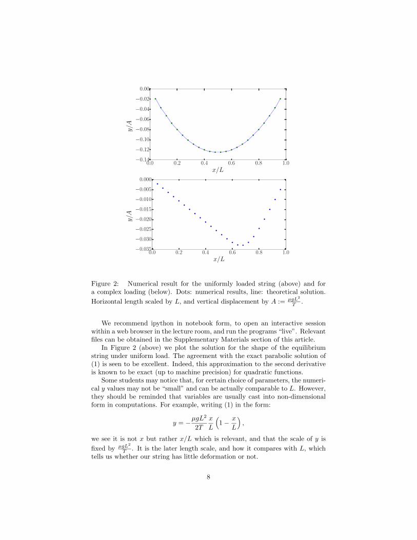
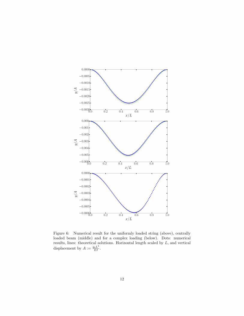
Figure 2: Numerical result for the uniformly loaded string (above) and fora complex loading (below). Dots: numerical results, line: theoretical solution.

Horizontal length scaled by L, and vertical displacement by A := µgL2

T .

We recommend ipython in notebook form, to open an interactive sessionwithin a web browser in the lecture room, and run the programs “live”. Relevantfiles can be obtained in the Supplementary Materials section of this article.

In Figure 2 (above) we plot the solution for the shape of the equilibriumstring under uniform load. The agreement with the exact parabolic solution of(1) is seen to be excellent. Indeed, this approximation to the second derivativeis known to be exact (up to machine precision) for quadratic functions.

Some students may notice that, for certain choice of parameters, the numeri-cal y values may not be “small” and can be actually comparable to L. However,they should be reminded that variables are usually cast into non-dimensionalform in computations. For example, writing (1) in the form:

y = −µgL2

2T

x

L

(1− x

L

),

we see it is not x but rather x/L which is relevant, and that the scale of y is

fixed by µgL2

T . It is the later length scale, and how it compares with L, whichtells us whether our string has little deformation or not.

8

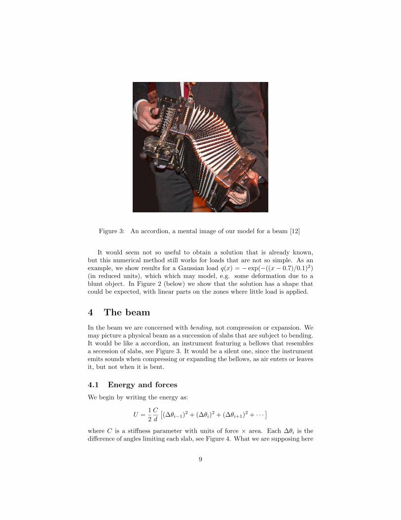
Figure 3: An accordion, a mental image of our model for a beam [12]

It would seem not so useful to obtain a solution that is already known,but this numerical method still works for loads that are not so simple. As anexample, we show results for a Gaussian load q(x) = − exp(−((x − 0.7)/0.1)2)(in reduced units), which which may model, e.g. some deformation due to ablunt object. In Figure 2 (below) we show that the solution has a shape thatcould be expected, with linear parts on the zones where little load is applied.

4 The beam

In the beam we are concerned with bending, not compression or expansion. Wemay picture a physical beam as a succession of slabs that are subject to bending.It would be like a accordion, an instrument featuring a bellows that resemblesa secession of slabs, see Figure 3. It would be a silent one, since the instrumentemits sounds when compressing or expanding the bellows, as air enters or leavesit, but not when it is bent.

4.1 Energy and forces

We begin by writing the energy as:

U =1

2

C

d

[(∆θi−1)2 + (∆θi)

2 + (∆θi+1)2 + · · ·]

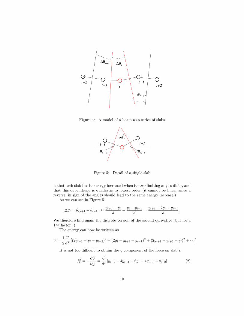
where C is a stiffness parameter with units of force × area. Each ∆θi is thedifference of angles limiting each slab, see Figure 4. What we are supposing here

9

∆θ

∆θ

ii−1i−2 i+1

i+2

∆θi

i+1

i−1

Figure 4: A model of a beam as a series of slabs

θ θ

i−1 i+1

∆θi

ii−1,i i,i+1

Figure 5: Detail of a single slab

is that each slab has its energy increased when its two limiting angles differ, andthat this dependence is quadratic to lowest order (it cannot be linear since areversal in sign of the angles should lead to the same energy increase.)

As we can see in Figure 5

∆θi = θi,i+1 − θi−1,i ≈yi+1 − yi

d− yi − yi−1

d=yi+1 − 2yi + yi−1

d.

We therefore find again the discrete version of the second derivative (but for a1/d factor. )

The energy can now be written as

U =1

2

C

d3[(2yi−1 − yi − yi−2)2 + (2yi − yi+1 − yi−1)2 + (2yi+1 − yi+2 − yi)2 + · · ·

]It is not too difficult to obtain the y component of the force on slab i:

fyi = −∂U∂yi

=C

d3[yi−2 − 4yi−1 + 6yi − 4yi+1 + yi+2] (2)

10

This is an approximation to the fourth derivative (but for a −1/d factor )[10]. Therefore:

f(x) ≈ −Cd∂4y

∂x4

4.2 The beam equation

It is again easy to add vertical forces to each slab:

U = · · · − F (x)y

The final dynamical equation is

m∂2y

∂t2= −Cd∂

4y

∂x4+ F,

and its static solution is given by:

C∂4y

∂x4=F

d= q

where q = F/d is the beam load. As shown in the Appendix A, the C parameteris C = EI, where E is Young’s modulus (again) and I a quantity known as thesecond moment of inertia. We therefore obtain the dynamic beam equation:

µ∂2y

∂t2= −EI ∂

4y

∂x4+ q

and its static version, which is probably better known:

EI∂4y

∂x4= q

4.3 Computing the loaded beam

Again, our discrete problem involving the slabs can be cast as a linear algebraproblem:

∇4~y = ~q,

with a fourth derivative matrix ∇4 having: a diagonal with −6 values, subdiag-onals above and below it with values of 4, and finally subdiagonals above andbelow the two former ones with values of −1, with a common factor of 1/d4, asseen in Equation (2).

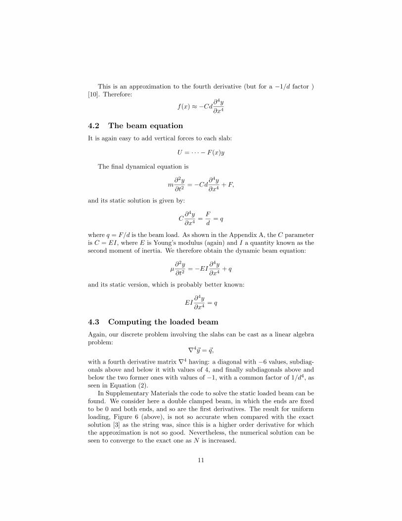
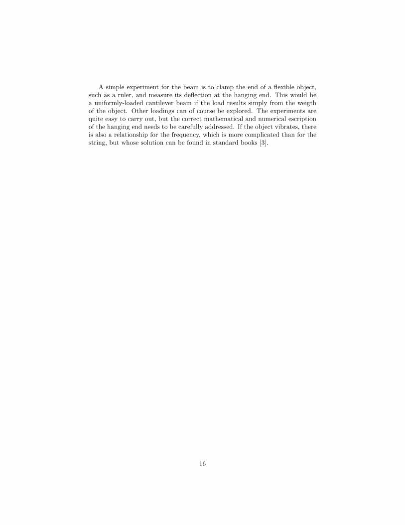
In Supplementary Materials the code to solve the static loaded beam can befound. We consider here a double clamped beam, in which the ends are fixedto be 0 and both ends, and so are the first derivatives. The result for uniformloading, Figure 6 (above), is not so accurate when compared with the exactsolution [3] as the string was, since this is a higher order derivative for whichthe approximation is not so good. Nevertheless, the numerical solution can beseen to converge to the exact one as N is increased.

11

0.0 0.2 0.4 0.6 0.8 1.0

x/L

−0.0030

−0.0025

−0.0020

−0.0015

−0.0010

−0.0005

0.0000

y/A

0.0 0.2 0.4 0.6 0.8 1.0

x/L

−0.006

−0.005

−0.004

−0.003

−0.002

−0.001

0.000

y/A

0.0 0.2 0.4 0.6 0.8 1.0

x/L

−0.0006

−0.0005

−0.0004

−0.0003

−0.0002

−0.0001

0.0000

y/A

Figure 6: Numerical result for the uniformly loaded string (above), centrallyloaded beam (middle) and for a complex loading (below). Dots: numericalresults, lines: theoretical solutions. Horizontal length scaled by L, and vertical

displacement by A := q0L4

EI .

12

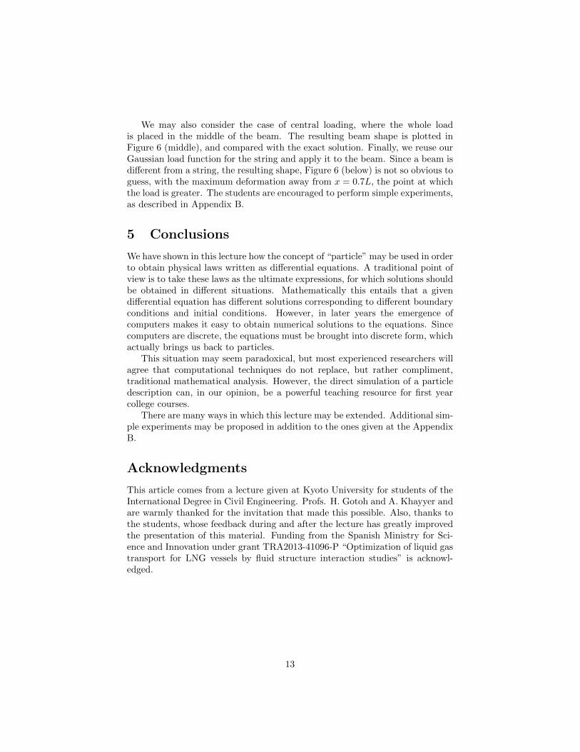
We may also consider the case of central loading, where the whole loadis placed in the middle of the beam. The resulting beam shape is plotted inFigure 6 (middle), and compared with the exact solution. Finally, we reuse ourGaussian load function for the string and apply it to the beam. Since a beam isdifferent from a string, the resulting shape, Figure 6 (below) is not so obvious toguess, with the maximum deformation away from x = 0.7L, the point at whichthe load is greater. The students are encouraged to perform simple experiments,as described in Appendix B.

5 Conclusions

We have shown in this lecture how the concept of “particle” may be used in orderto obtain physical laws written as differential equations. A traditional point ofview is to take these laws as the ultimate expressions, for which solutions shouldbe obtained in different situations. Mathematically this entails that a givendifferential equation has different solutions corresponding to different boundaryconditions and initial conditions. However, in later years the emergence ofcomputers makes it easy to obtain numerical solutions to the equations. Sincecomputers are discrete, the equations must be brought into discrete form, whichactually brings us back to particles.

This situation may seem paradoxical, but most experienced researchers willagree that computational techniques do not replace, but rather compliment,traditional mathematical analysis. However, the direct simulation of a particledescription can, in our opinion, be a powerful teaching resource for first yearcollege courses.

There are many ways in which this lecture may be extended. Additional sim-ple experiments may be proposed in addition to the ones given at the AppendixB.

Acknowledgments

This article comes from a lecture given at Kyoto University for students of theInternational Degree in Civil Engineering. Profs. H. Gotoh and A. Khayyer andare warmly thanked for the invitation that made this possible. Also, thanks tothe students, whose feedback during and after the lecture has greatly improvedthe presentation of this material. Funding from the Spanish Ministry for Sci-ence and Innovation under grant TRA2013-41096-P “Optimization of liquid gastransport for LNG vessels by fluid structure interaction studies” is acknowl-edged.

13

References

References

[1] Goodno Barry J. Gere, James M. Mechanics of materials, 2009.

[2] S P Timoshenko. History of strength of materials. McGraw-Hill New York,1953.

[3] J M Gere and S P Timoshenko. Mechanics of Materials. PWS PublishingCompany, 1997.

[4] George B. Arfken, Hans J. Weber, and Frank E. Harris. MathematicalMethods for Physicists. Academic Press, 6 edition, 2005.

[5] S. Patankar. Numerical Heat Transfer and Fluid Flow. Series in com-putational methods in mechanics and thermal sciences. Taylor & Francis,1980.

[6] Marcelo Alonso and Edward J Finn. Fundamental University Physics. Ad-dison Wesley, 1980.

[7] Paul Allen Tipler and Gene Mosca. Physics for scientists and engineers.W. H. Freeman, 2006.

[8] Hugh D Young, Roger A Freedman, and A Lewis Ford. Sears and Zeman-sky’s University Physics with Modern Physics. Addison-Wesley, 2011.

[9] Wolfgang Bauer and Gary Westfall. University Physics with ModernPhysics. McGraw-Hill, 2013.

[10] Samuel Daniel Conte and Carl W. De Boor. Elementary Numerical Analy-sis: An Algorithmic Approach. McGraw-Hill Higher Education, 3rd edition,1980.

[11] SciPy. SciPy web site. 2015. http://scipy.org [Online; accessed 21-July-2015].

[12] Bengt Nyman. Chris auxer on accordion, 2015. https://commons.

wikimedia.org/wiki/File:Chris_Auxer_on_accordion.jpg [Online;accessed 21-July-2015].

A The stiffness parameter

A slab is compressed in different amount at different values of y. Indeed thecompression (or extension) at height y is:

c = y∆θ y ∈ (−h/2, h/2).

14

x

yd

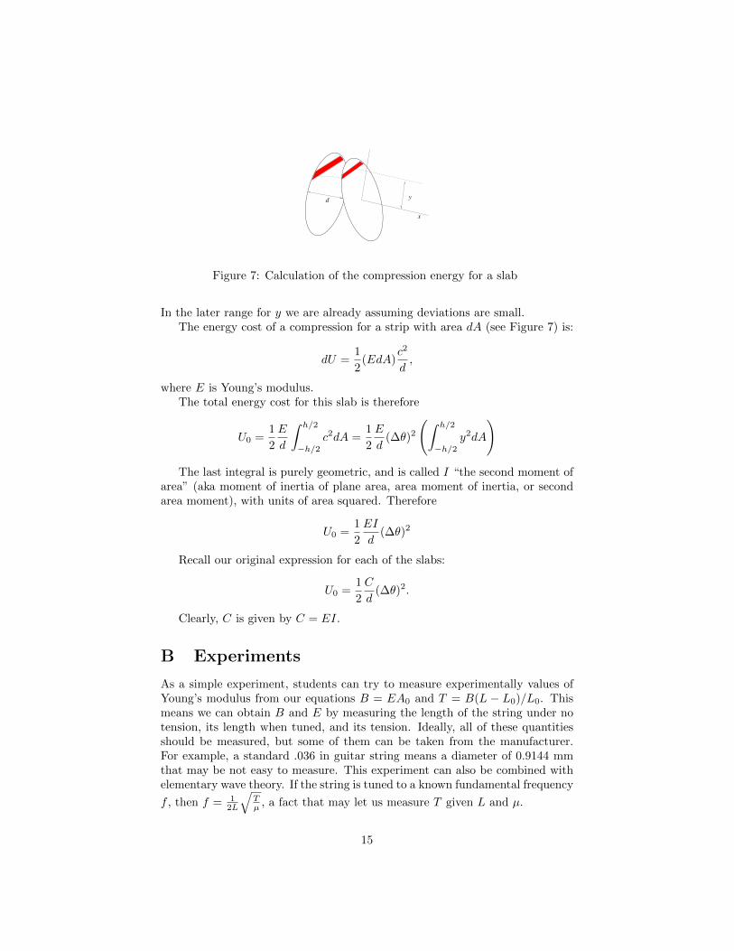
Figure 7: Calculation of the compression energy for a slab

In the later range for y we are already assuming deviations are small.The energy cost of a compression for a strip with area dA (see Figure 7) is:

dU =1

2(EdA)

c2

d,

where E is Young’s modulus.The total energy cost for this slab is therefore

U0 =1

2

E

d

∫ h/2

−h/2c2dA =

1

2

E

d(∆θ)2

(∫ h/2

−h/2y2dA

)The last integral is purely geometric, and is called I “the second moment of

area” (aka moment of inertia of plane area, area moment of inertia, or secondarea moment), with units of area squared. Therefore

U0 =1

2

EI

d(∆θ)2

Recall our original expression for each of the slabs:

U0 =1

2

C

d(∆θ)2.

Clearly, C is given by C = EI.

B Experiments

As a simple experiment, students can try to measure experimentally values ofYoung’s modulus from our equations B = EA0 and T = B(L − L0)/L0. Thismeans we can obtain B and E by measuring the length of the string under notension, its length when tuned, and its tension. Ideally, all of these quantitiesshould be measured, but some of them can be taken from the manufacturer.For example, a standard .036 in guitar string means a diameter of 0.9144 mmthat may be not easy to measure. This experiment can also be combined withelementary wave theory. If the string is tuned to a known fundamental frequency

f , then f = 12L

√Tµ , a fact that may let us measure T given L and µ.

15

A simple experiment for the beam is to clamp the end of a flexible object,such as a ruler, and measure its deflection at the hanging end. This would bea uniformly-loaded cantilever beam if the load results simply from the weigthof the object. Other loadings can of course be explored. The experiments arequite easy to carry out, but the correct mathematical and numerical escriptionof the hanging end needs to be carefully addressed. If the object vibrates, thereis also a relationship for the frequency, which is more complicated than for thestring, but whose solution can be found in standard books [3].

16