On the Derivation of the Slutsky Equationin Post War Microeconomics

Alan J. RogersDepartment of EconomicsUniversity of Auckland

(a.rogers@auckland.ac.nz)

June 2014

Abstract

This paper is concerned with the ways in which the Slutsky equation has beenderived in mainstream economics, primarily in the post war period. Also con-sidered are some related results for inverse, or indirect demands, the formalmathematical consideration of which goes back at least as far as Antonelli’s([1886] 1971) work on the integrability problem. The main point is that thetraditional approach, which was prevalent until the 1970’s, and which is essen-tially a streamlined version of the calculus-based approach of Pareto ([1927]1971) and Slutsky ([1915] 1953), can be instructive in ways that complementthe modern duality-based approach. The latter has come to monopolise main-stream consumer and producer treatments at the advanced undergraduate andgraduate levels and beyond. So far as the Slutsky equation and its analoguefor inverse demands are concerned, we argue that the traditional, or classical,approach need not be heavily algebraic, and makes transparent the conditionson preferences beyond the traditional smoothness assumptions required for thederivations of these equations: for direct demands these rule out too muchsmoothness in indifference curves, and for indirect demands suffi cient smooth-ness is indispensible. The modern approach based on duality arguments yieldsthe same two equations neatly and compactly, but leaves some important endsuntied.

1

1. Introduction

The primary purpose of this paper is to consider the ways in which the Slutskyequation and some related aspects of consumer theory have been derived intreatments of of consumer theory at the advanced undergraduate and graduatelevels in the post-war period. These approaches to the theory have becomepart of neo-classical microeconomic orthodoxy.The first of two main approaches, which is referred to in this paper as classi-

cal, is exemplified by Hicks (1946), Samuelson (1947), and later on by textbookssuch as Henderson and Quandt (1958), Allen (1966) and many others, as wellas the monograph by Katzner (1970). This approach proceeds by analysingthe first order conditions for the problems of maximising a consumer’s utilityfunction - assumed suffi ciently smooth - subject to a budget constraint, in orderto determine the effect of on the maximising choices of small changes in pricesand income. The last step, often made use of rather cumbersome argumentsinvolving determinants of certain matrices associated with differentials of firstorder conditions for the constrained optimisation problem. In fact this ap-proach was the same in essence as that adopted by Pareto ([1927] 1971) andSlutsky ([1915] 1953), and independently by Hicks and Allen (1934a, 1934b).1

The prevailing view is that this result, and others, can be much more easilyand elegantly obtained by means of the duality between the utility and expen-diture functions, with much of the early work on the latter due to Hicks (1956),MacKenzie (1958). For more on this approach, including some historical back-ground, see Diewert (1982). So far as the Slutsky equation itself is concerned,the use of this approach became widespread in the 1970’s following the simplederivation in Cook (1972), and subsequently in the influential text by Varian(1978).The triumph of the duality approach since then seems to have been complete.

Modern, comprehensive texts such as Mas-Colell, Whinston and Green (1995)and Jehle and Reny (2001) are unanimous that this is preferable, with the olderapproach typically not even mentioned as an alternative. A recent exceptionis Balasko (2011) and in places, Kreps (2013). Of course, one indisputableattraction of duality ideas is that they have many elegant and useful applicationssuch as those suggested early on by Diamond and McFadden (1974), Gorman(1976) and subsequently by many others.But what seems to have been ignored or forgotten in much of the literature

of the last forty years or so, is that it is possible to obtain almost all of therelevant results of modern consumer theory via the classical approach by meansof quite elementary mathematics, which certainly should be understandableby those nowadays deemed of capable of studying economics at the graduatelevel. Morever, the limitations of the classical approach are somewhat more

1Chipman and Lenfant (2002) provide considerable historical perspective, and the connec-tion between the work of Pareto and Slutsky is described by Dooley (1983). Schultz (1935)provides an early view and exposition of the work of Slutsky, Pareto, Hicks and Allen, anduses similar mathematics.

2

apparent than those of the modern alternative, including the conditions imposedon underlying preferences.This paper is organised as follows. In section 2 we review a classical, pre-

duality, way of deriving the Slutsky equation, including explicit considerationof conditions which ensure the differentiability of the compensated and ordi-nary demand functions. In section 3, some examples are considered whichillustrate what can happen when preferences do not satisfy the usual smooth-ness/curvature properties. In section 4, we consider analogous results, obtainedby traditional methods, to those in section 2 for indirect demand functions, andsee that the requisite smoothness/curvature properties of preferences differ, butin a way that has a quite clear interpretation. In section 5 we see how directand inverse demands are related in the "standard" case where the traditionalconditions of both section 2 and 4 are satisfied.In section 6 we turn to a consideration of the duality approach for both

direct and indirect demands and the connections between the two that emergeeasily under suitable conditions.Throughout we will be concerned with the limitations of two approaches.

This inevitably means a consideration of some technical issues, which turn out tocentre on the smoothness and curvature properties of the consumer’s preferences.However, the economic interpretations of these and their consequences are notdiffi cult to uncover and understand.The setting follows the postwar orthodoxy: the consumer chooses a con-

sumption bundles consisting of n goods and represented by an n × 1 vec-tor, x, in the non-negative orthant of n-dimensional Euclidean space (i.e.,Rn+); the consumer’s preferences have entirely conventional properties, includingmonotonicity and strict convexity, and are represented by a continuous utilityfunction, u(x), or simply u, which is everywhere continuous, strictly increas-ing, and, except where otherwise stated, strictly quasi-concave and smooth.The consumer’s optimisation problem is to choose x to maximise utility

subject to a conventional budget constraint: p′x ≤ y where y is income (ascalar) and p is a n × 1 vector of positive prices (so p ∈ Rn++). We alsoassume away the possibility of binding non-negativity contraints.2

It should be noted at the outset that, In part because the analysis in thispaper is based on assumed properties of a consumer’s preferences, we will notconsider the revealed preference approach to consumer demand introduced bySamuelson (1938) and subsequently the subject of considerable development andanalysis.3

In spite of the fact that much of the paper is concerned with some technical-ities and special cases, the discussion is rather informal with preference beinggiven for the most part to notational convenience over rigour.

2This point is important when it comes to differentiability of demand functions, as theexample of Kreps (2013, p.275) illustrates.

3This theory is formulated in terms of finite differences rather than in terms of the deriv-atives appearing in the Slutsky equation and elsewhere in the classical and duality basedaproaches. Obtaining differential versions of the main revealed preference results is some-times possible, but we will not pursue that idea here.

3

2. The Classical Approach

The consumer’s utility function u is assumed to possess continuous derivativesup to at least second order; the consumer’s optimisation problem is

maxx

u(x) subject to p′x ≤ y.

The solution for x to the constrained utility maximisation problem is denotedby x(p; y) (or simply x), and is the vector of ordinary, or Marshallian, demandfunctions. The first order conditions for an interior maximum are, as usual,

ux − λp = 0 (1)

y − p′x = 0

where ux ≡ ∂u(x)/∂x, (the n × 1 vector of marginal utilities) and λ is aLagrange multiplier. The conditons (1) are suffi cient for a local maximum if inaddition, u satisfies the second order condition

dx′Udx < 0 for each dx 6= 0 satisfying dx′ux = 0 (2)

where U is the Hessian matrix of u. The condition (2) is stated and usedby Slutsky ([1915] 1953) and has been widely invoked since.4 This conditionis important in what follows and is equivalent to strong (as opposed to strict)quasi-convexity of u, and implies non-zero Gaussian curvature of the indifferencecurves.5

It is important to note that this condition, i.e, (2), is stronger than requiredfor a solution for x to (1) to yield a local maximum: for example it is possible,in the absence of (2), for u be strictly quasi-concave, so that there is a uniqueutility maximising x for each p, as the example of Katzner (1968) illustrates.6

An alternative is to adopt the weaker condition

dx′Udx ≤ 0 for each dx satisfying dx′ux = 0 (3)

which we will have occasion to refer to.Note also that nonsingularity of U is, on its own, neither necessary nor

suffi cient for satisfaction of either (2) or (3): imposing this condition tends tolead, unecessarily, to messy algebraic manipulations which have probably donenothing to make the general approach outlined here digestible.7

4For example, explicitly by Hicks (1946) and Samuelson (1947), with the latter definingthis as a condition for a "regular" relative constrained maximum. See also Allen’s (1935)exposition and discussion of Slutsky’s paper.

5See, for example Barten and Bohm (1982), Malinvaud (1972), Debreu (1972), Mas-Collel(1985).

6This and related examples are considered in more detail in the next section. The under-lying idea for his case is very simple: the usual second derivative condition is suffi cient butnot necessary for a local maximum. For example, the function f(z) = −z4 is uniquely max-imised at z = 0, but there the second derivative vanishes. Neverthless the set {y, z|y ≤ f(z)}is strictly convex and f is strictly concave. See also Katzner (1970).

7For example, Brown and Deaton (1973) assume non-singularity of U , and appear torecommend monotone transformations of u which achieve this in order to obtain explicitformulae for the components of a partitioned inverse of U.

4

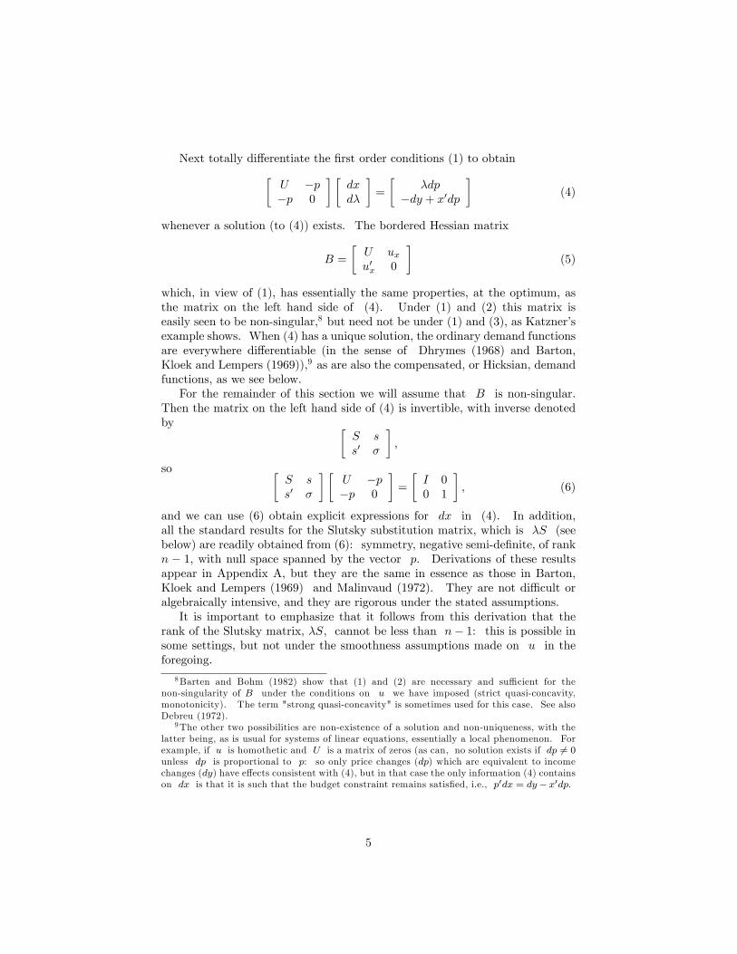
Next totally differentiate the first order conditions (1) to obtain[U −p−p 0

] [dxdλ

]=

[λdp

−dy + x′dp

](4)

whenever a solution (to (4)) exists. The bordered Hessian matrix

B =

[U uxu′x 0

](5)

which, in view of (1), has essentially the same properties, at the optimum, asthe matrix on the left hand side of (4). Under (1) and (2) this matrix iseasily seen to be non-singular,8 but need not be under (1) and (3), as Katzner’sexample shows. When (4) has a unique solution, the ordinary demand functionsare everywhere differentiable (in the sense of Dhrymes (1968) and Barton,Kloek and Lempers (1969)),9 as are also the compensated, or Hicksian, demandfunctions, as we see below.For the remainder of this section we will assume that B is non-singular.

Then the matrix on the left hand side of (4) is invertible, with inverse denotedby [

S ss′ σ

],

so [S ss′ σ

] [U −p−p 0

]=

[I 00 1

], (6)

and we can use (6) obtain explicit expressions for dx in (4). In addition,all the standard results for the Slutsky substitution matrix, which is λS (seebelow) are readily obtained from (6): symmetry, negative semi-definite, of rankn − 1, with null space spanned by the vector p. Derivations of these resultsappear in Appendix A, but they are the same in essence as those in Barton,Kloek and Lempers (1969) and Malinvaud (1972). They are not diffi cult oralgebraically intensive, and they are rigorous under the stated assumptions.It is important to emphasize that it follows from this derivation that the

rank of the Slutsky matrix, λS, cannot be less than n− 1: this is possible insome settings, but not under the smoothness assumptions made on u in theforegoing.

8Barten and Bohm (1982) show that (1) and (2) are necessary and suffi cient for thenon-singularity of B under the conditions on u we have imposed (strict quasi-concavity,monotonicity). The term "strong quasi-concavity" is sometimes used for this case. See alsoDebreu (1972).

9The other two possibilities are non-existence of a solution and non-uniqueness, with thelatter being, as is usual for systems of linear equations, essentially a local phenomenon. Forexample, if u is homothetic and U is a matrix of zeros (as can, no solution exists if dp 6= 0unless dp is proportional to p: so only price changes (dp) which are equivalent to incomechanges (dy) have effects consistent with (4), but in that case the only information (4) containson dx is that it is such that the budget constraint remains satisfied, i.e., p′dx = dy− x′dp.

5

Note also that under (1) and (2), U can be singular but cannot have rankless than n− 1, since if it did, B would be singular.10

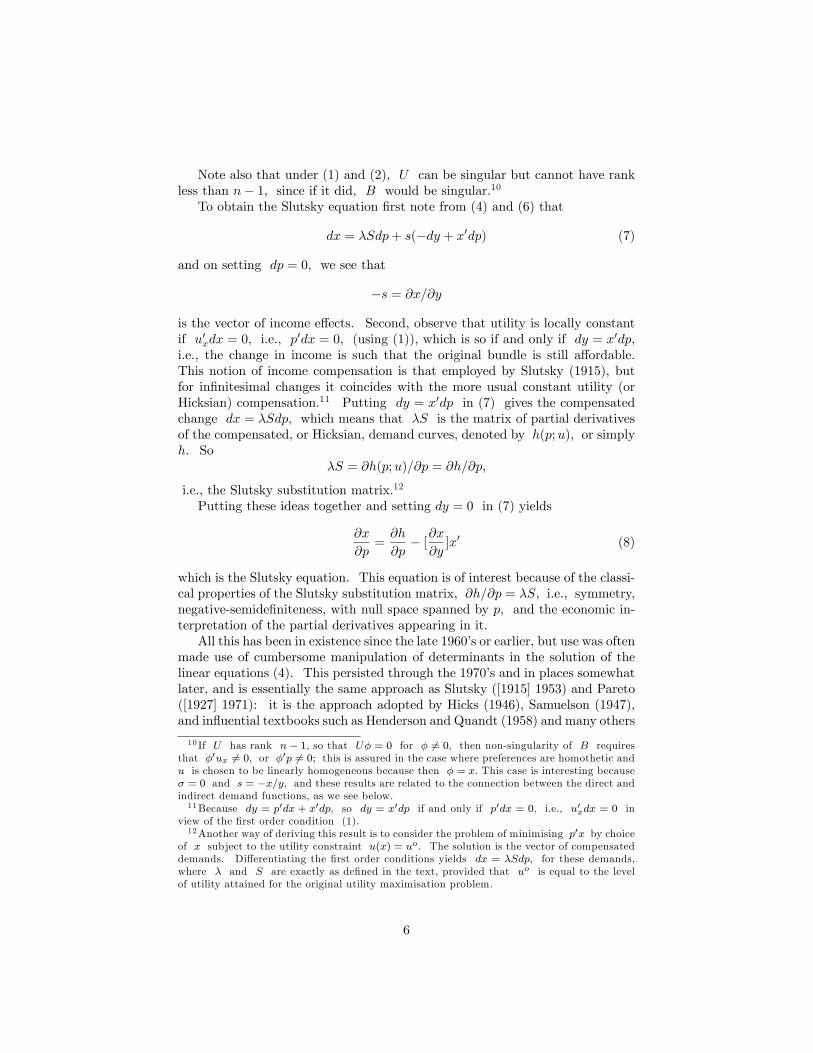
To obtain the Slutsky equation first note from (4) and (6) that

dx = λSdp+ s(−dy + x′dp) (7)

and on setting dp = 0, we see that

−s = ∂x/∂y

is the vector of income effects. Second, observe that utility is locally constantif u′xdx = 0, i.e., p′dx = 0, (using (1)), which is so if and only if dy = x′dp,i.e., the change in income is such that the original bundle is still affordable.This notion of income compensation is that employed by Slutsky (1915), butfor infinitesimal changes it coincides with the more usual constant utility (orHicksian) compensation.11 Putting dy = x′dp in (7) gives the compensatedchange dx = λSdp, which means that λS is the matrix of partial derivativesof the compensated, or Hicksian, demand curves, denoted by h(p;u), or simplyh. So

λS = ∂h(p;u)/∂p = ∂h/∂p,

i.e., the Slutsky substitution matrix.12

Putting these ideas together and setting dy = 0 in (7) yields

∂x

∂p=∂h

∂p− [

∂x

∂y]x′ (8)

which is the Slutsky equation. This equation is of interest because of the classi-cal properties of the Slutsky substitution matrix, ∂h/∂p = λS, i.e., symmetry,negative-semidefiniteness, with null space spanned by p, and the economic in-terpretation of the partial derivatives appearing in it.All this has been in existence since the late 1960’s or earlier, but use was often

made use of cumbersome manipulation of determinants in the solution of thelinear equations (4). This persisted through the 1970’s and in places somewhatlater, and is essentially the same approach as Slutsky ([1915] 1953) and Pareto([1927] 1971): it is the approach adopted by Hicks (1946), Samuelson (1947),and influential textbooks such as Henderson and Quandt (1958) and many others

10 If U has rank n− 1, so that Uφ = 0 for φ 6= 0, then non-singularity of B requiresthat φ′ux 6= 0, or φ′p 6= 0; this is assured in the case where preferences are homothetic andu is chosen to be linearly homogeneous because then φ = x. This case is interesting becauseσ = 0 and s = −x/y, and these results are related to the connection between the direct andindirect demand functions, as we see below.11Because dy = p′dx + x′dp, so dy = x′dp if and only if p′dx = 0, i.e., u′xdx = 0 in

view of the first order condition (1).12Another way of deriving this result is to consider the problem of minimising p′x by choice

of x subject to the utility constraint u(x) = uo. The solution is the vector of compensateddemands. Differentiating the first order conditions yields dx = λSdp, for these demands,where λ and S are exactly as defined in the text, provided that uo is equal to the levelof utility attained for the original utility maximisation problem.

6

including, somewhat surprisingly, the unpublished lecture notes by McFaddenand Winter (1968) 13 .For later reference we note that the vector of "income effects", −s, are, as

usual, identical to the effects of a suitable scaling of prices, with income, y, heldconstant, since if we set dp = −pdκ for a scalar κ 14 we obtain dx = −sx′pdκusing Sp = 0 so that −s = y∂x/∂κ, or

−s = ∂x/∂κ,

if we adopt the normalisation y = 1, noting that ∂xi/∂κ is non-negative ifthe ith good is normal. Then (8) takes the form

∂x

∂p=∂h

∂p− [

∂x

∂κ]x′.

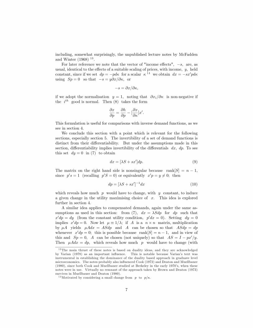
This formulation is useful for comparisons with inverse demand functions, as wesee in section 4.We conclude this section with a point which is relevant for the following

sections, especially section 5. The invertibility of a set of demand functions isdistinct from their differentiability. But under the assumptions made in thissection, differentiability implies invertibility of the differentials dx, dp. To seethis set dy = 0 in (7) to obtain

dx = [λS + sx′]dp. (9)

The matrix on the right hand side is nonsingular because rank[S] = n − 1,since p′s = 1 (recalling p′S = 0) or equivalently x′p = y 6= 0; then

dp = [λS + sx′]−1dx (10)

which reveals how much p would have to change, with y constant, to inducea given change in the utility maximising choice of x. This idea is exploredfurther in section 4.A similar idea applies to compensated demands, again under the same as-

sumptions as used in this section: from (7), dx = λSdp for dp such thatx′dp = dy (from the constant utility condition, p′dx = 0). Setting dy = 0implies x′dp = 0. Now let µ ≡ 1/λ; if A is a n× n matrix, multiplicationby µA yields µAdx = ASdp and A can be chosen so that ASdp = dpwhenever x′dp = 0; this is possible because rank[S] = n− 1, and in view ofthis and Sp = 0, A can be chosen (not uniquely) so that AS = I − px′/y.Then µAdx = dp, which reveals how much p would have to change (with

13The main thrust of these notes is based on duality ideas, and they are acknowledgedby Varian (1978) as an important influence. This is notable because Varian’s text wasinstrumental in establishing the dominance of the duality based approach in graduate levelmicroeconomics. The notes probably also influenced Cook (1972) and Deaton and Muellbauer(1980), since both Cook and Muellbauer studied at Berkeley in the early 1970’s, when thesenotes were in use. Virtually no remnant of the approach taken by Brown and Deaton (1973)survives in Muellbauer and Deaton (1980).14Motivated by considering a small change from p to p/κ.

7

y constant) to induce a given utility preserving change in x. One choice of Awhich has some appeal is the reflexive generalised inverse of S because, likeS, it is symmetric, negative semidefinite and of rank n− 1.15

3. Examples

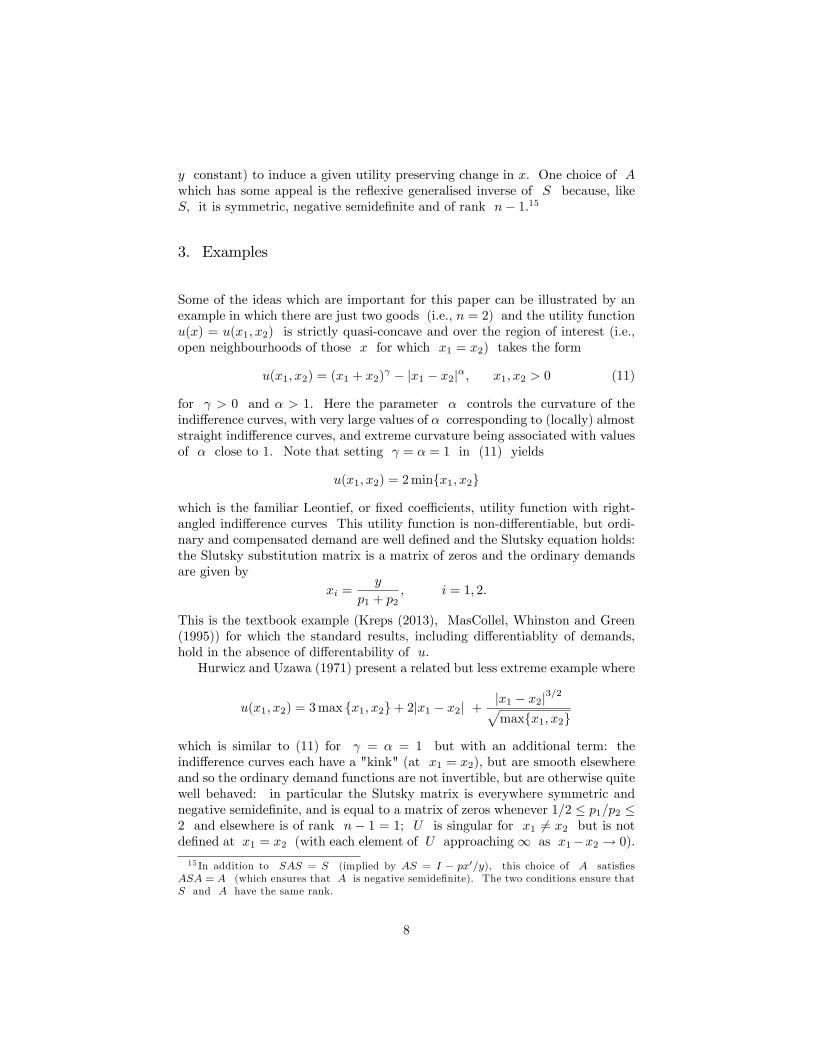
Some of the ideas which are important for this paper can be illustrated by anexample in which there are just two goods (i.e., n = 2) and the utility functionu(x) = u(x1, x2) is strictly quasi-concave and over the region of interest (i.e.,open neighbourhoods of those x for which x1 = x2) takes the form

u(x1, x2) = (x1 + x2)γ − |x1 − x2|α, x1, x2 > 0 (11)

for γ > 0 and α > 1. Here the parameter α controls the curvature of theindifference curves, with very large values of α corresponding to (locally) almoststraight indifference curves, and extreme curvature being associated with valuesof α close to 1. Note that setting γ = α = 1 in (11) yields

u(x1, x2) = 2 min{x1, x2}

which is the familiar Leontief, or fixed coeffi cients, utility function with right-angled indifference curves This utility function is non-differentiable, but ordi-nary and compensated demand are well defined and the Slutsky equation holds:the Slutsky substitution matrix is a matrix of zeros and the ordinary demandsare given by

xi =y

p1 + p2, i = 1, 2.

This is the textbook example (Kreps (2013), MasCollel, Whinston and Green(1995)) for which the standard results, including differentiablity of demands,hold in the absence of differentability of u.Hurwicz and Uzawa (1971) present a related but less extreme example where

u(x1, x2) = 3 max {x1, x2}+ 2|x1 − x2| +|x1 − x2|3/2√max{x1, x2}

which is similar to (11) for γ = α = 1 but with an additional term: theindifference curves each have a "kink" (at x1 = x2), but are smooth elsewhereand so the ordinary demand functions are not invertible, but are otherwise quitewell behaved: in particular the Slutsky matrix is everywhere symmetric andnegative semidefinite, and is equal to a matrix of zeros whenever 1/2 ≤ p1/p2 ≤2 and elsewhere is of rank n − 1 = 1; U is singular for x1 6= x2 but is notdefined at x1 = x2 (with each element of U approaching∞ as x1−x2 → 0).

15 In addition to SAS = S (implied by AS = I − px′/y), this choice of A satisfiesASA = A (which ensures that A is negative semidefinite). The two conditions ensure thatS and A have the same rank.

8

Nevertheless, the demand curves possess continuous derivatives everywhere withrespect to both prices and income.16

Returning to (11), consider the case where α ∈ (1, 2). Then there is nokink in the indifference curves, both ordinary and compensated demands arecontinuous, differentiable, and the Slutsky matrix is a matrix of zeros wheneverx1 = x2, but with the usual rank n − 1 behaviour elsewhere (with elementseach converging to zero as x1−x2 → 0). The Slutsky equation as before holdseverywhere. The utility function is not twice differentiable where x1 = x2.

The standard case is obtained by setting α = 2 in (11): u is twicecontinuously differentiable everywhere (in the relevant neighbourhood), U isof constant rank, and S is everywhere of rank n− 1.17

But if α > 2, the compensated and ordinary demand functions are notdifferentiable (at x for which x1 = x2). The matrix B is singular; the Slutskyequation does not hold because the Slutsky matrix is not defined. Katzner’s(1968) example, where

u(x1, x2) = x31x2 + x1x32

coincides with (11) for γ = α = 4.The standard results hold for α = 2 in (10) but also more generally,

when there is neither too little nor too much curvature: in such cases secondderivatives exist and do not exhibit a particular type of degeneracy. The exactcharacterisation of this condition on curvature is non-singularity of the matrixB.One question which emerges from the foregoing is the following. Suppose

demand functions are such that the Slutsky matrix is well defined and every-where of rank n − 1 (as well as being symmetric and negative semi-definite),then does this imply smoothness of u? The answer appears to be yes, at leastlocally, see Blackorby and Diewert (1979). Such conditions on S are equiva-lent to quite strong restrictions on the curvature properties of the expenditurefunction, so we return to this question in section 6.

4. Inverse Demands

Here we consider the inverse, or indirect demand functions. Antonelli ([1886]1971) used these explicitly in his work on the integrability problem, i.e, condi-tions on a set of inverse demand functions which ensure that they are consistentwith maximisation of a utility function with the usual properties. See alsoSamuleson (1947), Chipman (1971) and Cornes (1992) for more on his work.The key idea in this context is that observed price ratios provide information

16The important point from the point of view of Hurwicz and Uzawa is that the integrabilityconditions hold, i.e., the direct demand functions satisfy conditions which are suffi cient toguarantee recoverability of the utility function from direct demands, without requiring thatthese be uniquely invertible.17For example, if γ = 1 , then U has rank 1 (and is therefore singular), while if γ = 2,

U is non-singular.

9

on marginal rates of substitution, so if enough is known about the consumer’sinverse demands, his preferences can be recovered from them.Here we confine attention to the properties of the inverse demand functions

under assumptions on the utility function made in the last section, and so theanalysis has the same traditional utility-based flavour, and the same startingpoint. We will be particularly concerned with an analogue of the Slutskyequation, and properties of the Antonelli matrix, which is the analogue of theSlutsky matrix for inverse demands. These are somewhat easier to obtain thanthe results of the last section, and more importantly, their derivation makes useof weaker assumptions. The derivations below are classical in spirit, are quitestraightforward, but do not feature in the literature, perhaps because, whereinverse demands are considered, it is typically alongside direct demands. (Forexample in Samuelson (1947), Salvas-Bronsard et al (1977); and also, althoughin a less classical spirit, Cornes (1996), Jehle and Reny (2001).)Here we take a consumption bundle x, and obtain prices p and income y

which support this in the sense that, given them, x maximises utility. If thefirst order conditions (1) are satisfied we can write

λ =x′uxy

by using y = p′x. Thenx′uxy

p = ux (12)

which on division by x′ux/y gives the inverse demands, p(x; y), explicitlyin term of x and y, and is sometimes referred to as the Hotelling-Woldidentity. Clearly the utility function needs to be differentiable for (12) to makesense, but if so it is clear that the inverse demands in (12) are unique. TheLeontief and Hurwicz-Uzawa examples outlined in the last section show howuniqueness can fail in the absence of differentiability of u. These derivatives(of u) need not themselves be continuous, or differentiable, and if they are not,the inverse demand functions will not generally be differentiable. To see thisconsider the example (11) of the last section with α ∈ (1, 2): then the inversedemands are not differentiable at x for which x1 = x2. The intuition hereis clear: small movements in x away from such points induce large changesin p because of the sharp curvature of indifference curves at these points.Additional smoothness in u yields further results, including differentiability ofthe demands in question, so, as for the previous section, we assume that u istwice continuously differentiable.In what follows it is notationally convenient to let

µ ≡ y/(x′ux) and y = 1;

the first simply is an abreviation (equivalent to setting µ = 1/λ) and thesecond is a normalisation, adopted because concern is with the effect of changesin x on the vector p/y. Totally differentiate (12) and rearrange slightly to

10

obtainUdx = x′uxdp+ px′Udx+ pu′xdx

or,dp = µ [I − px′]Udx− µpu′xdx (13)

which gives dp uniquely for given dx without any assumption beyond suffi cientdifferentiability of u. Next replace u′x in (13) with p′/µ, add and subtractµ[I − px′]Uxp′dx from both sides of (13), and rearrange to obtain

dp = µ[[I − px′]U [I − xp′] dx+ µ{[I − px′]Uxp′ − pp′/µ]}dx. (14)

Suppose that dx is such that utility is constant, so p′dx = 0. Then the secondterm on the right hand side of (14) vanishes, and

dp = µAdx (15)

whereA ≡ [I − px′]U [I − xp′]. (16)

In (15), µA is the Antonelli matrix18 , since the change in x leaves util-ity unchanged and and so the inverse demands in question are compensatedinverse demand functions, which we denote by the vector a(x; v); thereforeµA = ∂a(x; v)/∂x. The Antonelli matrix is the analogue, for inverse demands,of the Slutsky matrix, and has similar properties. It is symmetric, negativesemidefinite, and has rank no greater than n − 1, and its null space containsx. Symmetry and the rank result are obvious19 and negative semidefinitenessis a simple consequence of (16) and (3), as shown in Appendix B.Note in passing that a simple negativity result for compensated demands

can also be easily obtained. This is dx′dp ≤ 0, for any utility preservingchange in x, since from (13), p′dx = 0 implies

dx′dp = µdx′Udx

which is non-positive by (3). This result is implied by negative semi-definitenessof A, but is not suffi cient for it. (It does not, for example, imply, as doesnegative semidefiniteness, that the diagonal elements of A are non-positive.)

To obtain an analogue of the Slutsky equation for inverse demands considerthe effect on p of scaling x, by changing from x to x/δ so in (14) setdx = −xdδ where δ is a positive scalar. Then Adx = 0, because Ax = 0,and, from (14),

dp = µ{[I − px′]Uxp′ − pp′/µ}(−xdδ),18This term for the substitution matrix for a set of inverse demand functions was apparently

first used by Samuelson (1947).19Symmetry because of the symmetry of U , and Ax = 0, simply because [I − xp′]x = 0

uner the normalisation y = 1.

11

so, using ux = p/µ and p′x = 1 yields

∂p/∂δ = −µ{[I − px′]Ux− p/µ}p′x= −b

whereb ≡ µ{[I − px′]Ux− p/µ}.

Using this in (14) yieldsdp = [µA+ bp′]dx (17)

or∂p

∂x=∂a

∂x− [

∂p

∂δ]p′ (18)

which is an analogue of (8) for inverse demands. Here the Antonelli matrixappears in place of the Slutsky matrix, with prices and quantities interchanged,and the income effect (or equivalently, the effect of scaling prices) is replaced bythe effect of scaling quantities.The scale effect (∂p/∂x) in (18) (or b in (17)) gives the effect on p

of a scaling in x so it can be expected to take a simple form when pref-erences are homothetic. This is so, since, in this case, Ux = 0, implying∂p/∂δ = −b = p. A similar result holds for direct demands under the samecondition on preferences. In this case the geometry of the scale effects for thetwo types of (uncompensated) demands is identical, but that is not the case fornon-homothetic preferences, since for direct demands scaling of prices alwayspreserves, up to scale, the vector ux, and this is not in general accompaniedby a scaling of quantites, while for inverse demands, scaling of quantities is notaccompanied by scaling of ux or prices.20 .The main result is here is that (18) holds, and that the Antonelli matrix is

symmetric, negative semidefinite, of rank at most n − 1, and its null spacecontains x. These results are obtained from (1), (3) and twice continuousdifferentiability of u.21 Obtaining the same results under weaker conditionsseems unlikely to be easily achievable, because the vector of inverse demandsis essentially the vector of first partial derivatives of the utility function, sodifferentiablity of the former is almost equivalent to differentiability of the latter.Notice also that in the foregoing the Antonelli matrix is not required to have

maximum rank (n − 1), nor is there any counterpart of the requirement insection 2 that B be non-singular. But rank[A] = n − 1 is both necessaryand suffi cient for the invertibility of the differentials dp and dx in the un-compensated and compensated inverse demands, as can be established by using20Notice also that [I − px′]∂p/∂δ = µ[I − px′]Ux since [I − px′]p = 0 under the

normalisation p′x = 1, and I−px′ is an idempotent matrix. This provides an interpretationof the component of the scale effect on prices in the non-homethetic case; and the twocomponents of the vector ∂p/∂δ, −µ[I − px′]Ux and p, are orthogonal. A similardecomposition can be obtained for direct demands under the conditions of section 2. We canwrite ∂x/∂y = −[I−xp′]s−xp′s, with the two components being orthogonal, while xp′s = xfrom (6); in the homothetic case, s = −x, the first of the two components vanishes.21 If the condition (3) is replaced by (2), then the rank of A is n − 1 , and the results

obtained are entirely analogous to those of section 2.

12

arguments similar to those at the end of section 2. (A derivation appears inAppendix B.) In fact, in this case, the Slutsky equation, and the propertiesof its constituent parts, can be obtained entirely from the results given above.This result, and its converse, are considered in the next section.This point is important because it suggests that if A has rank less than

n− 1, the direct demands will not be differentiable and the Slutsky matrix willnot be defined, under the differentiability assumptions on u adopted in thissection. In fact, the non-singularity of B and the condition rank[A] = n − 1turn out to be equivalent, as shown in Appendix C. So, if rank[A] = n − 1,the results of this section must be consistent with those of section 2, and in factthey mirror those results in a natural way, as we see in the next section.We conclude this section by returning to the example due to Katzner (1968),

mentioned in the last section. For x, p such that x1 = x2 > 0, p1 = p2 theelements of U take the same non-zero value , and it easy to verify that A = 0in this case, so rank[A] = 0 = n − 2; here B is singular (of rank n = 2),and so S is not defined. The indifference curves have so little curvature nearthe points under consideration that small movements in x induce no changesin p. Or, in terms of compensated direct demands, small changes in p resultin changes in x so large that the derivatives of these demand curves are notdefined.Similar results hold for similar reasons in (11) with α > 2, the simplest

being that for which γ = 1: then U = 0, so A = 0, and B is singular. Inthe case where 1 < α < 2, the elements of U are not defined (are infinite)at x for which x1 = x2; there the compensated inverse demands are notdifferentiable, again because small changes in x induce very large changes inp.

5. The Standard Case.

Here we are concerned with the relationship between the differentials of directand inverse (or indirect) demands. So we confine attention to situations inwhich both are defined.

The assumptions made initially are those of section 2, including non-singularity of the matrix B in (5). Then S and A of sections 2 and 4are defined and each have rank n − 1. At the end of section 2 we saw thatthe differentials of the direct demands can be inverted, and for consistency werequire that the demands so obtained coincide with those of section 4.For uncompensated demands we require from (9) and (17) that [λS + sx′]

and [µA+ bp′] be inverses of each other, i.e.,

[λS + sx′][µA+ bp′] = I (19)

and this can be seen to hold from the definitions of S, s, A, b in sections 2 and4.22

22The matrix on the left hand side of (19) is SA + λSbp′ + sx′bp′, using µ = 1/λ and

13

For compensated demands we require that, for utility preserving changes inx, dx = λSdp and dp = µAdx i.e., dx = µλSAdx, or, in view of µ = 1/λ,

[I − SA]dx = 0 whenever p′dx = 0.

This follows from postmultiplication of (19) by dx, or from the definitions ofA and S. Similarly, dp = µAdx = ASdp whenever x′dp = 0 (an implicationof the constant utiity condition p′dx = 0 and the normalisation on y). So werequire that

[I −AS]dp whenever x′dp = 0

and this can also be verified from (19) or from the definitions.The fact that S and A are reflexive generalised inverses of each other

also follows from (19), since postmultiplication by S yields S = SAS andpremultiplication by A yields A = ASA.Next we see how the Slutsky equation and its properties can be obtained

from knowledge of the Antonelli equation, and its properties, however thesehave been derived, provided the Antonelli matrix has rank n − 1, as well asbeing symmetric and negative semi-definite. Denote it by µA where µ isa scalar, and recall that Ax = 0. We can write dx = λSdp where S ischosen to be a reflexive generalised inverse of A and λ ≡ 1/µ. This choiceof generalised inverse ensures that λS is negative semidefinite, symmetric andhas rank n−1, like µA. Moreover, the null space of S is spanned by p sincep′dx = λp′Sdp = 0 whenever p′dx = 0, i.e., for all dp such that x′dp = 0,and this implies p′S = 0, as required. Therefore λS has the properties ofthe Slutsky matrix.The differentials for the uncompensated demands can be inverted23 to yield

dx = [µA+ bp′]−1dp and we write

[µA+ bp′]−1 = λS + ∆.

Here ∆dp = 0 whenever x′dp = 0 (which holds when utility and income areconstant), which implies that ∆ has rank equal to one, and therefore can bewritten ∆ = γx′. It remains to show that γ is equal to −∂x/∂y. Setdp = pdk where k is a scalar so dx = [λS + ∆]pdk = γx′pdk = γdk (usingλSp = 0 and x′p = 1). Then γ = ∂x/∂k, or the vector of income effects−∂x/∂y, because of the equivalence of the effects on the utility maximisingchoices of x of decreases in income and equiproportionate increases in pricesnoted at the end of section 2. This yields the Slutsky equation (8).Parallel arguments can be employed to obtain (17) from the Slutsky equation

(8) on the assumption that S in that equation has maximum rank, n − 1,as well as being symmetric and negative semi-definite, again regardless of how

x′A = 0. From the definition of b, x′b = −x′p = −1, so sx′bp′ = −sp′. And, also from thedefinition of b, Sb = µSUx, so λSbp′ = SUxp′, since µ = 1/λ. Now, SU − sp′ = I from(6) so SUxp′ = xp′ + sp′. So the matrix in question is SA+ xp′. From the definition of A,and Sp = 0, SA = SU [I − xp′] = [I + sp′][I − xp′] = I − xp′, which yields the result.23Because µA + bp′ can have rank less than n − 1 only if bp′x = 0, i.e., only if b = 0,

which is impossible under the usual local non-satiation assumption.

14

these properties have been obtained. The analog of ∆ for the present casealso has rank one and is of the form γp′ where now γ = ∂p/∂δ, the effect ofscaling x on p, is obtained from setting dx = xdk, so dp = [µA+γp′]xdk =γdk.The arguments given above rely on the condition that the ranks of A, S be

n − 1 It is possible for either the Slutsky or Antonelli equation to hold in itsabsence, but apparently not both.The final point to be made in this section concerns the two matrices[

S xx′ 0

],

[A pp′ 0

]. (20)

in which Sp = 0 and Ax = 0. These are nonsingular if and only if S and Aeach have rank n− 1, with null spaces spanned by p and x respectively.24

And if S, A are reflexive generalised inverses, the bordered matrices in (20)are inverses of each other, given the normalisation y = 1.25 So there is anappealing symmetry between the matrices in (20) and another sense in which Aand S are counterparts, as are also p and x. See Salvas-Bronsard et al (1976)and Stern (1986). The matrices in (20) are also associated with optimisationproblems which are related to the one we have been concerned with, as we seein the next section.

6. Duality

The duality approach in microeconomics is based on the theory of convex sets,and makes use of the fact that such sets can be described by their tangentplanes (or supporting hyperplanes). See Diewert (1982) for a survey of thedevelopment of the theory.26 The sets in the case of consumer theory of mostinterest are the upper contour sets {x : u(x) ≥ v} which here are assumedclosed and strictly convex. This implies that a utility function, u, whichrepresents these preferences is strictly quasi-concave, as we have assumed in thepreceding sections.The expenditure function is defined by

e(p; v) = minxp′x subject to u(x) ≥ v

24This is so since if the first of these is singular, then Sc + xd = 0 and x′c = 0, withc 6= 0 and/or d 6= 0; then c′Sc = 0, implies that c is proportional to p if S has rankn−1. This is impossible in view of x′c = 0. Conversely, if rank of S is less than n−1, thefirst bordered matrix in (20) must be singular. The argument for A an the second borderedmatrix in (20) follows the same lines.25Let SA+ xp′ = I + C. Then SAS = S +CS and ASA = A+AC. Also x = x+Cx,

using p′x = 1, and p′ = p′ + p′C. So CS = 0, Cx = 0 and AC = 0, p′C = 0. HenceC = 0 by the non-singularity of the bordered matrices in (20).26Early work was done by Hotelling, Wold, Roy. The expenditure function in consumer

theory is due to Hicks (1956) and McKenzie (1958), and the analogous construct in producertheory is due to Shephard (1953). A succinct recent perspective on some of the technicalaspects is given by Blume (2008).

15

and is the least cost of attaining utility v at prices p. It is equal to p′h(p; v)where h(p; v) is the expenditure minimising consumption bundle, or vectorof compensated demands. The expenditure function is quite easily seen to beconcave in p, and to possess the "derivative property" (otherwise known asShephard’s Lemma)

∂e(p; v)/∂p = h(p; v). (21)

So the vector of partial derivatives of the expenditure function is simply thevector of compensated demands. This an example of one of the appeals of theduality approach.27 Moreover the existence of the derivatives in (20) dependsonly on the uniqueness of the expenditure minimising x. This is remarkable inview of the identity e(p; v) = p′h(p; v): differentiability of the left hand sidemight be expected to require differentiability of its components on the righthand side.28 The ordinary and compensated demands coincide, as usual, whenappropriately evaluated, and in particular,

x(p, e(p; v)) = h(p; v). (22)

Now partially differentiate both sides with respect to p using the chain rule toobtain

∂x/∂p+ [∂x/∂y][∂e/∂p]′ = ∂h/∂p (23)

or, using x = h = ∂e/∂p,

∂x

∂p=∂h

∂p− [

∂x

∂y]x′

which is the Slutsky equation (8), recalling that ∂h/∂p is the Slutsky matrix,which we will denote by So in this section. It remains to establish the sym-metry and negative semidefiniteness of ∂h/∂p: the former follows from Young’stheorem and the assumed continuous differentiablity of h, while negative semi-definiteness follows from concavity of the expenditure function in p for fixedv.29 Finally, the rank of So is no greater than n− 1, and p lies in the nullspace of So, because the expenditure minimising x (i.e, h(p; v)) is invariantwith respect to scaling of p, for given utility, v.This is very neat and straightforward once the properties of the expenditure

function have been understood. But the Slutsky equation is a statement aboutderivatives of compensated and uncompensated demand functions and the argu-ment given above simply assumes that these derivatives exist. Katzner’s (1968)

27A similar property (Roy’s identity) holds for the indirect utility function and ordinary(uncompensated) demands. It is possible to base a derivation of the Slutsky equation onRoy’s identity, but the usual - and simpler - approach is via the expenditure function, asoutlined in htis section.28The idea here is that if po, p∗ are two price vectors and xo, x∗ are the associated (unique)

expenditure minimising consumption bundles, e(p∗; v) = p∗′x∗ ≤ p∗′xo and e(po; v) =po′xo ≤ po′x∗, so (p∗−po)′x∗ ≤ e(p∗; v)−e(po; v) ≤ (p∗−po)′xo; then divide by ||po−p∗||and take limits to obtain the desired differentiability.29Concavity follows from the inequality e(p; v) ≤ p′x for any x for which u(x) ≥ v, with

equality for x = h(p; v).

16

example and that in (11) (for a > 2) serve as reminders that this is not assured,even when underlying preferences have quite conventional properties.30

And, even if the second partial derivatives of the expenditure function existand are continuous, so that the above argument concerning the Slutsky matrix isvalid, this says nothing about the income effects, and in particular the existenceof the derivatives ∂x/∂y.31

The examples of Blackorby and Diewert (1979) reveal that an expenditurefunction which, for fixed v, is concave, homogenous of degree zero and continu-ously differentiable in p, and strictly increasing in v, may have associated withit a utility function which does not exhibit all of the usual properties of strictquasi-concavity, continuity and local non-satiation. Blackorby and Diewert’sfirst example is

e(p; v) =

{vp1 for 0 ≤ v ≤ 1p1 + (v − 1)p2 for v > 1

(for p1, p2 > 0). This is interesting in the present context because ordinarydemands are not everywhere differentiable, while the compensated demands donot depend on prices, and so all elements of the Slutsky matrix are zero. Thelast feature can be expected to arise whenever e(p; v) exhibits little curva-ture. (A related example is used by Rubinstein (2006) in a Giffen good con-text.) Another example in this context is Blackorby and Diewert’s third examplee(p; v) = v(p1 + p2), for which the utility function is the fixed coeffi cients, orLeontief, case mentioned in section 3: u(x1, x2) = min {x1, x2}. Indeed this isan important example of the advantage of the duality/expenditure function ap-proach: substitution effects are obtained here without the non-differentiabilityof the utility function getting in the way. A less extreme example is a linearlyhomogeneous version of Katzner’s example, adapted to an expenditure function:

e(p; v) = v[p31p2 + p1p

32

]1/4.

This has the usual properties of an expenditure function, but all second deriva-tives vanish at p for which p1 = p2, so that all elements of the Slutsky matrix

30The last sentence of Proposition 3 theorem of Diamond and McFadden (1978), says that ifu is twice continuously differentiable and B is non-singular, then the Hessian matrix of theexpenditure function is twice continuously differentiable and has rank n− 1. This is is oneimplication of section 2, and is essentially classical in flavour. A weaker conclusion is providedin the first sentence: the Hessian of e(p; v) exists, is symmetric and negative semidefinitefor almost all positive prices whenever a utility maximising vector exists everywhere (and ispresumably unique).31A similar point in a different context is made by Hurwicz and Uzawa (1971): integrability

of a set of (uncompensated) demand functions is obtained by imposing conditions on theincome effects as well on the matrix of subsitution effects. For more on the connection betweenconcepts of smoothness of preferences and smoothness of ordinary and compensated demandfunctions, see Neilson (1991) and Debreu (1972): for the latter only smoothness/curvaturealong indifference curves matters, while the former requires smoothness over the indifferencemap.

17

are zero at such p. This expenditure function is nevertheless strictly quasiconcave in p for fixed v.Some of the more theoretical work on duality, such as Krishna and Son-

nenschein (1990) and Jackson (1986), has emphasized restrictions on classes ofexpenditure functions and utility functions which are such that there is a one-to-one correspondence between members of each class. This is sometimes knownas the "duality problem" because once the correspondence has been established,it is possible to work with either type of function according to convenience, cer-tain in the knowledge of the properties of its partner in the other class, withouthaving to derive those properties explicitly.It would be convenient to have similar results for the differentiability proper-

ties of expenditure and utility functions. Some have been obtained by Blackorbyand Diewert (1979): these state that, locally, a "standard" set of second orderdifferentiability properties of the expenditure function implies and is implied by"standard" behaviour of the utility function.But this does reveal what non-standard behaviour of the expenditure func-

tion implies for the utility function, and conversely. For example, if e(p; v) istwice differentiable in p and its Hessian has rank less than n − 1, u(x) isprobably not twice differentiable; conversely, if u(x) is not twice differentiable,the Slutsky matrix may be defined, but if so probably has rank less than n− 1.Leaving this point aside, another argument in favour of the duality approach

is that it allows easy, parallel derivations for inverse demands by means of the"distance function" whose popularity in consumer theory seems due primarilyto Gorman (1976). This is defined by

d(x; v) = maxδ{u(x/δ) ≥ v}

i.e., for given x and given level of utility v, d(x; v) is the amount by whichx must be scaled so that the scaled commodity bundle, x/δ, yields utilityv.32 It is another way of representing preferences, noting in particular thatd(x; v) = 1 defines the indifference curve corresponding to utility v, (sinced(x; v) = 1 if and only if u(x) = v). Therefore, the expenditure function maybe defined in terms of d instead of u as

e(p; v) = minxp′x subject to d(x; v) ≥ 1. (24)

Instead of deriving the properties of the distance function from scratch, it isconvenient to make use of the relation

d(x; v) = minpp′x subject to e(p; v) ≥ 1 (25)

as in Gorman (1976), and also Deaton (1979), Cornes (1995). One way ofobtaining (25) is as follows. Take an arbitrary x, p, v with p scaled so that

32This defintion is essentially the same as that of the "gauge function" defined by McFadden(1978); see also Rockafellar (1970). Weymark (1980) uses the term "transformationfunction"; the idea has a long history in the analysis of production technologies.

18

e(p; v) = 1 33 and choose δ so that u(x/δ) = v. Then e(p; v) ≤ p′x/δ, sod(x; v)e(p; v) ≤ p′x since d(x; v) = δ from the definition of d and the choiceof δ. Therefore d(x; v) ≤ p′x/e(p; v) = p′x which yields (25); noting that theinequality d(x; v) ≤ p′x holds as an equality when x/δ is the least cost way ofattaining v at prices proportional to p. This last point is important becauseit is the reason why the solution for p in (25) is the vector of compensatedinverse demands, given x and v.Once (24) and (25) have been established, it is possible to exploit the fact

that d has exactly analogous properties as e: the derivative property is∂d/∂x = a(x; v), i.e., the vector of compensated inverse demands, and andwhenever it is defined, the Hessian of d(x; v), ∂2d(x;u)/∂x∂x′, is symmetricnegative semidefinite, of rank at most n−1, with x contained in its null space.So we obtain classical results for the Antonelli matrix, since it is precisely thisHessian, and we denote it in this section by Ao.To obtain an analogue of the Slutsky equation for inverse demands requires

defining the uncompensated demands in such a way that the properties of thedistance function can be further exploited. The (vector of) uncompensatedinverse demands is written p(x; δ): as before, this is the price vector whichsupports x/δ as the utility maximising choice when income (y) is equal toone; p(x; δ) is clearly homogeneous of degree zero in x and δ.Compensated and uncompensated inverse demands coincide when suitably

evaluated: specifically, p(x; δ) = a(x; v) when δ is such that u(x/δ) = v,or, equivalently,

p(x; d(x; v)) = a(x; v).

Now differentiate both sides with respect to x, use ∂d(x; v)/∂x = a(x; v), andevaluate at δ = 1, (so v = u(x)) to obtain

∂p

∂x=∂a

∂x− [

∂p

∂δ]a′

which is (17) of section 4, once a in the second matrix on the right han sideis replaced by p, and the scale effect is again given by the vector ∂p/∂δ,evaluated at δ = 1.Since the distance function is just another of representing a preference or-

dering, it shares many of the properties of a utility function used for the samepurpose. So differentiability can be an issue: for the Leontief example con-sidered briefly in section 2, the distance function is not differentiable, so thederivative property does not hold. 34 And, the existence of second derivativescan also be problematical. In (11), for example, this fails for the case γ =α ∈ (1, 2), so Ao is not defined. This is not surprising in view of the resultsof section 4, since in this case the utility function is not twice differentiable.Now we turn to the connection between Ao and So. Apply the derivative

33This scaling is harmless because e(p; v) is homogeneous of degree one in p.34Which simply reflects the fact that the (normalised) price vector which support an eco-

nomically relevant consumption bundle is not unique.

19

property twice to each of e(p; v) and d(x; v) to obtain, as in Deaton (1979),

h(p; v) = h(∂d(x; v)/∂x; v) = ∂e(∂d(x; v)/∂x; v)/∂p (26)

a(x; v) = a(∂e(p; v)/∂p; v) = ∂d(∂e(p; v)/∂p; v)/∂x; (27)

differentiating the first of these with respect to p then yields So = SoAoSo,and the second with respect to x yields Ao = AoSoAo, once we evaluate thederivatives in question at e(p;u) = y = 1, (a scale normalisation on prices)and δ = 1 (a scale normalisation on quantities).This is very neat, but does not give much insight into the economic inter-

pretation of the relationship between So and Ao, including the question ofthe invertibility of the differentials dx and dp discussed in the last section.The derivatives in question obviously must exist for this argument to be valid,but in addition Ao and So must have maximum rank, n− 1, something thatis not at all obvious from the argument just given, but which should be clearfrom the last section, if the elements of these matrices are to be interpreted aspartial derivatives of a consumer’s compensated direct and inverse demands.One way of thinking about this last point is to note that the first order

conditions for (24)p+ λo∂d(x; v)/∂x = 0

where λo is a Lagrange multiplier; here the derivative property gives∂d(x; v)/∂x = a(x; v), so λo = 1, and totally differentiating this and theconstraint d(x; v) = 1, applying the derivative property again along withAo = ∂2d(x; v)/∂x∂x′ (and so assuming differentiability of compensated inversedemands) yields [

Ao pp′ 0

] [dxdλo

]=

[dp0

]. (28)

If we pursue this approach, differentiability of direct compensated demand func-tions requires that the matrix on the left hand side of (28) be non-singular, whichrequires that the rank of Ao be n−1. Observe the similarity between (28) and(4) if for the latter we consider compensated demands by setting dy = x′dp.This is is not surprising because for compensated direct demands the problemis equivalent to minimising expenditure subject to a utility constraint, and thisproblem therefore differs from that in (28) only in the way the utility constraintis represented.If we proceed in the same way with the optimisation problem (25), we obtain

the first order condition x + µo∂e(p; v)/∂p = 0, where µo is a Lagrangemultiplier, and this and the constraint e(p; v) = 1 yields µo = 1, and(assuming the differentiability of compensated direct demands),[

So xx′ 0

] [dpdµo

]=

[dx0

]. (29)

In (29), differentiability of indirect demands using this approach requires thatSo have rank n− 1.

20

The matrices on the left hand sides of (28) and (29) are inverses of eachother, when these exist. Under this condition we can obtain the generalizedinverse connection between Ao and So given above, and we can obtain (28)and (29) from each other, and so obtain the relationships between dx anddp for the two types of compensated demands. Again this is neat, and thesymmetries are appealing, but we have seen from section 4 that approachingindirect demands this way imposes restrictions on consumer preferences thatcan obscure some fundamental differences between the two types of demandfunctions.

Conclusion

Katzner (1970), whose book is squarely in the classical tradition, notes that thedistinguishing feature of that approach is that it is based on utility maximisa-tion in the presence of certain restrictions, including smoothness of the utilityfunction chosen to represent the consumer’s preference ordering. The smooth-ness assumption usually takes the form of a twice continuous differentiabilityassumption, and is usually adopted for analytical convenience. Kreps (2013,p.276), for example, has noted that while many economists find it unobjection-able, "it is also without any serious axiomatic basis". The modal approach inthe modern literature, on the other hand, is to adopt axioms on a preferenceordering such as completeness, continuity, monotonicity, and convexity of uppercontour sets, and then proceed to obtain from these properties of the expendi-ture function. This gives the impression that the older approach makes use ofan unnecessary, clumsy, ill-motivated assumption for the sake of some tediousalgebraic manipulations which can be avoided by adopting duality arguments.35

This may be true of some results, but there are others, such as the Slutsky equa-tion for direct demands and its analogue for indirect demands, where quite tidy,self-contained arguments can be constructed along entirely classical lines in sucha way that the role of the smoothness/curvature assumptions used is entirelyapparent.The disadvantage of the duality approach to the Slutsky equation is that

the latter is a statement about derivatives of compensated and uncompensateddemand functions, and duality methods are not conspicuously useful in estab-lishing the differentiablity of these demand functions.36 The strength of duality

35Deaton (1979, p.396) comments: "[m]uch of the power of duality methods comes fromtheir ability to replace mechanical matrix inversion by elementary algebra with economicinterpretations". Note, though, that there are no such inversions in section 4. Cornes (1992)also rejoices in the absence of "bordered Hessians" in the duality approach: neverthless, thereare occasions where they do arise quite naturally, as we have seen in (28) and (29) in the lastsection. And the critical curvature condition of section 2 is precisely the non-singularity ofthe bordered Hessian, B.36For example, Kreps (2013) obtains non-singularity of the bordered B as suffi cient for

differentiablity of ordinary direct demand functions; this derivation has a decidedly classicalflavour (c.f. Dhrymes (1967) , Barten et al. (1969)). The approach of section 2 makes itclear that this issue should be confronted at some stage, and in section 2 this is done prior toa consideration of the Slutsky equation.

21

methods, as Krishna and Sonnenschein (1990) note, is the use of functions (in-cluding the expenditure function and distance function) whose first derivativesare demand curves. But it is less helpful when it comes to the second deriv-atives of those functions. When this issue is taken seriously (as, for example,in Kreps(2013), Mas-Collel (1985)) the analysis often ends up having a classicallook. And one reason for taking that issue seriously is the connection betweenthe Slutsky results (especially symmetry and negative semi-definiteness of theSlutsky substitution matrix) and the integrability problem, i.e., the extent ofthe restrictions imposed on observable behaviour by the utility maximisationhypothesis.

Appendix A

Properties of S.

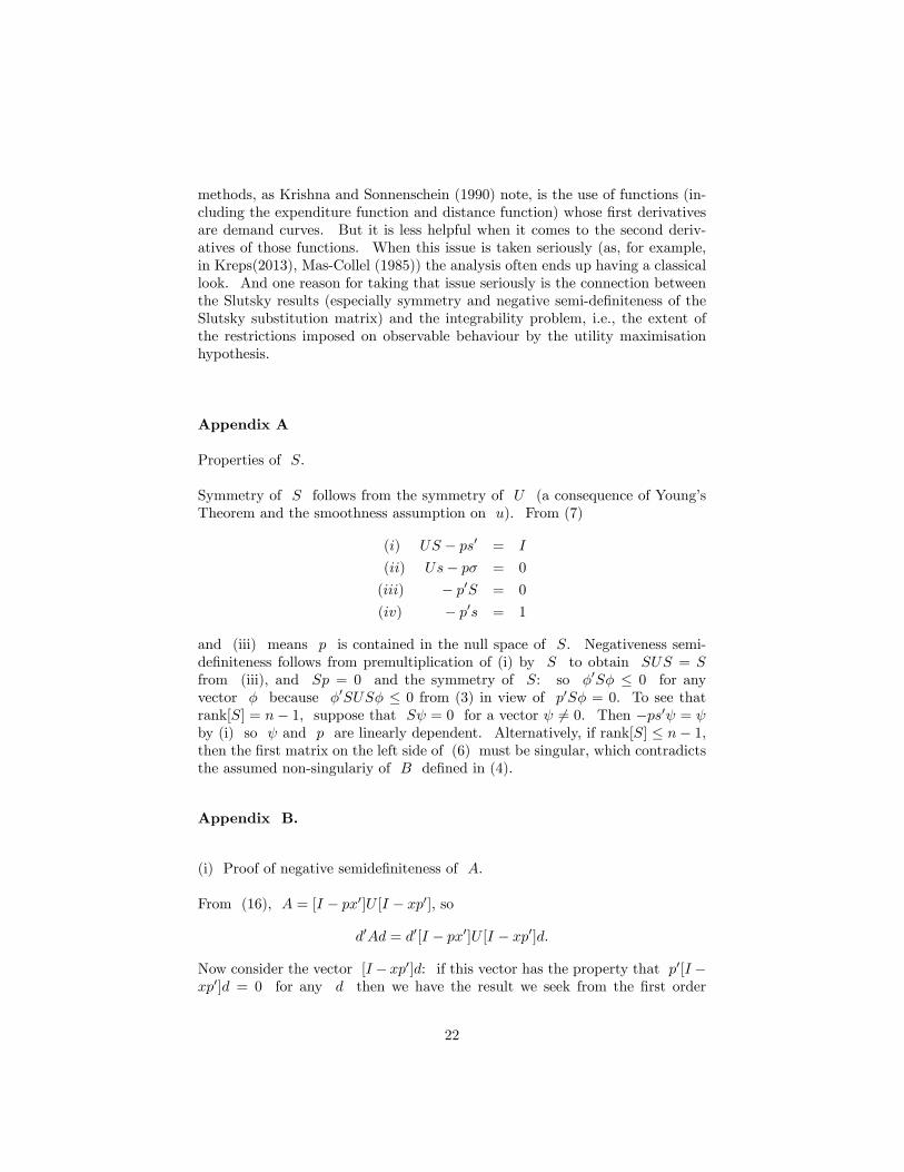
Symmetry of S follows from the symmetry of U (a consequence of Young’sTheorem and the smoothness assumption on u). From (7)

(i) US − ps′ = I

(ii) Us− pσ = 0

(iii) − p′S = 0

(iv) − p′s = 1

and (iii) means p is contained in the null space of S. Negativeness semi-definiteness follows from premultiplication of (i) by S to obtain SUS = Sfrom (iii), and Sp = 0 and the symmetry of S: so φ′Sφ ≤ 0 for anyvector φ because φ′SUSφ ≤ 0 from (3) in view of p′Sφ = 0. To see thatrank[S] = n− 1, suppose that Sψ = 0 for a vector ψ 6= 0. Then −ps′ψ = ψby (i) so ψ and p are linearly dependent. Alternatively, if rank[S] ≤ n− 1,then the first matrix on the left side of (6) must be singular, which contradictsthe assumed non-singulariy of B defined in (4).

Appendix B.

(i) Proof of negative semidefiniteness of A.

From (16), A = [I − px′]U [I − xp′], so

d′Ad = d′[I − px′]U [I − xp′]d.

Now consider the vector [I − xp′]d: if this vector has the property that p′[I −xp′]d = 0 for any d then we have the result we seek from the first order

22

condition (1) and the utility maximisation condition (3). But p′[I − xp′] = 0simply in view of p′x = y = 1.

(ii) Proof that rank[A] = n − 1, is both necessary and suffi cient for the in-vertibility the differentials dp and dx for uncompensated and compensatedinverse demands.

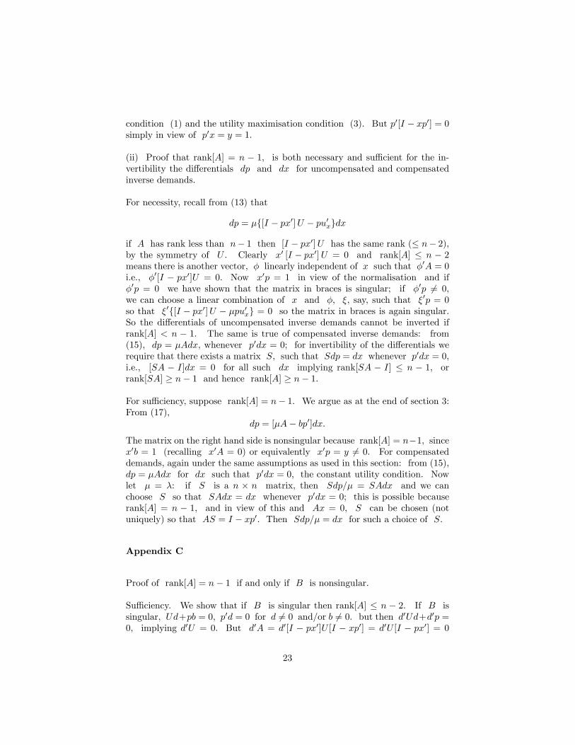
For necessity, recall from (13) that

dp = µ{[I − px′]U − pu′x}dx

if A has rank less than n− 1 then [I − px′]U has the same rank (≤ n− 2),by the symmetry of U . Clearly x′ [I − px′]U = 0 and rank[A] ≤ n − 2means there is another vector, φ linearly independent of x such that φ′A = 0i.e., φ′[I − px′]U = 0. Now x′p = 1 in view of the normalisation and ifφ′p = 0 we have shown that the matrix in braces is singular; if φ′p 6= 0,we can choose a linear combination of x and φ, ξ, say, such that ξ′p = 0so that ξ′{[I − px′]U − µpu′x} = 0 so the matrix in braces is again singular.So the differentials of uncompensated inverse demands cannot be inverted ifrank[A] < n − 1. The same is true of compensated inverse demands: from(15), dp = µAdx, whenever p′dx = 0; for invertibility of the differentials werequire that there exists a matrix S, such that Sdp = dx whenever p′dx = 0,i.e., [SA − I]dx = 0 for all such dx implying rank[SA − I] ≤ n − 1, orrank[SA] ≥ n− 1 and hence rank[A] ≥ n− 1.

For suffi ciency, suppose rank[A] = n− 1. We argue as at the end of section 3:From (17),

dp = [µA− bp′]dx.

The matrix on the right hand side is nonsingular because rank[A] = n−1, sincex′b = 1 (recalling x′A = 0) or equivalently x′p = y 6= 0. For compensateddemands, again under the same assumptions as used in this section: from (15),dp = µAdx for dx such that p′dx = 0, the constant utility condition. Nowlet µ = λ: if S is a n × n matrix, then Sdp/µ = SAdx and we canchoose S so that SAdx = dx whenever p′dx = 0; this is possible becauserank[A] = n − 1, and in view of this and Ax = 0, S can be chosen (notuniquely) so that AS = I − xp′. Then Sdp/µ = dx for such a choice of S.

Appendix C

Proof of rank[A] = n− 1 if and only if B is nonsingular.

Suffi ciency. We show that if B is singular then rank[A] ≤ n − 2. If B issingular, Ud+pb = 0, p′d = 0 for d 6= 0 and/or b 6= 0. but then d′Ud+d′p =0, implying d′U = 0. But d′A = d′[I − px′]U [I − xp′] = d′U [I − px′] = 0

23

because d′p = 0. Hence d′A = 0. Now if d 6= 0 we have a contradictionbecause p′d = 0 implies that d has both positive and negative elements, whichmeans that d and x are linearly independent, and since x′A = 0 it followsthat rank[A] ≤ n−2. If d = 0 then b = 0, because of Ud = 0, contradictingthe singularity of B.

Necessity. If rank[A] ≤ n− 2, then φ′A = 0 for φ linearly independent of xand or φ′[I − px′]U [I − xp′] = 0, or d′U = 0 for d′ = [φ′ − (φ′p)x′]. But ifUd = 0 then B is nonsingular only if d′p 6= 0; but this cannot be true sinced′p = φ′p− (φ′p)x′p = 0 in view of x′p = 1.

References

Allen, RG.D. (1935-36) "Professor Slutsky’s Theory of Consumer’s Choice",Review of Economic Studies, 3, 120-129.Allen, R.G.D. (1966). Mathematical Economics, 2nd ed. London: MacMillan.Antonelli, G. B. ([1886] 1971). Sulla Teoria Matematica della Economia Po-litica. Pisa: Nella Tipognafia del Folchetto. English translation by J.S.Chipman and A.P. Kirman (with revisions by W. Jaffe) in Chipman et al (1971),333-360.Balasko, Yves (2011). General Equilibrium Theory of Value. Princeton:Princeton University Press.Barton, A.P. and V. Bohm (1982). "Consumer Theory". In K.J. Arrow andM.D. Intriligator, eds, Handbook of Mathematical Economics. Amsterdam:North Holland. 387-429.Barton, A.P., T Kloek, and F.B. Lempers (1969). "A Note on a Class ofUtility and Production Functions Yielding Everywhere Differentiable DemandFunctions", Review of Economic Studies, 36, 109-111.Blackorby, C. and W.E. Diewert (1979). "Expenditure Functions, Local Du-ality, and Second Order Approximations", Econometrica 47, 579-602.Blume, L.E. (2008). "Duality." In S.N. Durlauf and L.E. Blume (eds) The NewPalgrave Dictionary of Economics 2nd ed. Basingstoke: Palgrave MacMillan.Brown, A. and A. Deaton (1973). "Surveys of Applied Economics: Modelsof Consumer Behavior", Economic Journal 82, 1145-1236. Reprinted inRoyal Economic Society and The Social Research Council Surveys of AppliedEconomics, Vol I (1973), 177-268.Cook, P. (1972). "A ’One Line’Proof of the Slutsky Equation", AmericanEconomic Review, 62, 139.Cornes, R. (1992). Duality and Modern Economics. Cambridge: CambridgeUniversity Press.Chipman, J.S. (1971). "Introduction to Part II" in Chipman et al (1971),114-148.

24

Chipman, J.S., L. Hurwicz, M. Richter, and H. Sonnenschein (eds) (1971). Pref-erences, Utility and Demand. New York: Harcourt Brace Jovanovich.Chipman, J.S. and J.-S. Lenfant (2002). "Slutsky’s 1915 Article: How it Cameto be Found and Interpreted", History of Political Economy, 34, 553-597.Deaton, A. (1979). "The Distance Function in Consumer Behaviour with Appli-cations to Index Numbers and Optimal Taxation", Review of Economic Studies,46 391-405.Deaton, A. and J. Muellbauer (1980). Economics and Consumer Behavior.Cambridge: Cambridge University Press.Debreu, G. (1972). "Smooth Preferences", Econometrica, 40, 603-615.Dhrymes, P. (1967). "On a Class of Utility and Production Functions YieldingEverywhere Differentiable Demand Functions", Review of Economic Studies,34 399-408.Diewert, W.E. (1982) "Duality Approaches in Microeconomic Theory". InK.J. Arrow and M.D. Intriligator, eds, Handbook of Mathematical Economics.Amsterdam: North Holland. 535-599.Diamond P. and D. McFadden (1974). "Some uses of the Expenditure Functionin Public Economics," Journal of Public Economics 3, 3-21.Dooley, P.C. (1983). "Slutsky’s Equation is Pareto’s Solution", History ofPolitical Economy, 15, 513-517.Gorman, W. (1976). "Tricks with Utility Functions". In M.J. Artis and A.R.Nobay (eds), Essays in Economic Analysis. Cambridge: Cambridge UniversityPress.Henderson, J.M. and R.E. Quandt (1958). Microeconomic Theory: A Mathe-matical Approach. New York: McGraw-Hill.Hicks, J.R. (1946). Value and Capital, 2nd edition. Oxford: OxfordUniversity Press.Hicks, J. R., (1956). A Revision of Demand Theory. Oxford: Oxford Univer-sity Press.Hicks, J. R., and R.G.D. Allen (1934a). "A Reconsideration of the Theory ofValue. Part I. Economica ns 1, 52-73.Hicks, J. R., and R.G.D. Allen (1934b). "A Reconsideration of the Theory ofValue. Part II. A Mathematical Theory of Individual Demand Functions",Economica, new series 1, 196-219.Hurwicz, L. and H. Uzawa (1971). "On the integrability of Demand Functions".In J. S. Chipman et al, 114-148.Jackson, M. O. (1986b). "Continuous Utility Functions in Consumer Theory:A Set of Duality Theorems", Journal of Mathematical Economics, 15, 63-77.Jehle, G.A. and P.J. Reny (2001). Advanced Microeconomic Theory 3rd ed.Boston: Addison Wesley.Katzner, D. W. (1968). "A Note on the Differentiability of Consumer DemandFunctions", Econometrica 36, 415-418.Katzner, D. W. (1970). Static Demand Theory. New York: Macmillan.Kreps, D. (2013). Microeconomic Foundations I. Princeton: Princeton Uni-versity Press.

25

Krishna, V., and H. Sonnenschein (1990). "Duality in Consumer Theory", inJ. Chipman, D. McFadden and M. Richter (eds), Preferences, Uncertainty andOptimality, Boulder: Westview Press, 44-55.Malinvaud, E. (1972). Lectures on Microeconomic Theory. Amersterdam:North Holland.Mas-Colell, A. (1985). The Theory of General Economic Equilibrium: ADifferentiable Approach. Cambridge: Cambridge University Press.Mas-Colell, A., M.D. Whinston and J.R. Green (1995). Microeconomic Theory.Oxford: Oxford University Press.McFadden, D., and S.G. Winter (1968). Consumer Theory. UnpublishedLecture Notes.McKenzie, L. (1957). "Demand Theory without a Utility Index", Review ofEconomic Studies, 24, 185-189.Neilson, W. S. (1991). "Smooth Indifference Sets", Journal of MathematicalEconomics, 20, 181-197.Pareto, V. ([1927] 1971). Manual of Political Economy. Translation by A.S.Schwier of the French edition of 1927. London: MacMillan.Rockafellar, R.T. (1970). Convex Analysis. Princeton: Princeton UniversityPress.Rubinstein, A. (2006). Lecture Notes on Microeconomic Theory. Princeton:Princeton University Press.Salvas-Bronsard, L., D., LeBlanc and C. Bronsard (1977). "Estimating DemandEquations: The Converse Approach", European Economic Review, 9, 301-321.Samuelson, P.A. (1938) "A Note on the Pure Theory of Consumer’s Behaviour",Economica, 61-72.Samuelson, P.A. (1947). Foundations of Economic Analysis. Cambridge:Harvard University Press.Shephard (1953). Cost and Production Functions. Princeton: Princeton Uni-versity Press.Schultz, H. (1935). "Interrelations of Demand, Price and Income", Journal ofPolitical Economy, 43, 433-481.Slutsky, E. E. ([1915] 1953). "Sulla Teoria del Bilancio del Consumatore",Giornale delgi Economisti 51, 1-26. English translation by O. Ragusa in K.E.Boulding and G.J. Stigler AEA Readings in Price Theory. London: GeorgeAllen and Unwin, 27-56.Stern, N. (1986). "A Note on Commodity Taxation: The Choice of Variableand the Slutsky, Hessian and Antonelli Matrices (SHAM)," Review of EconomicStudies 53, 293-299.Varian, H. (1978). Microeconomic Analysis. New York: Norton.Weymark, J.A. (1980). "Duality Results in Demand Theory", European Eco-nomic Review 14, 377-395.

26