Journal of Hydrology 526 (2015) 196–207

Contents lists available at ScienceDirect

Journal of Hydrology

journal homepage: www.elsevier .com/locate / jhydrol

A multi-model and multi-index evaluation of drought characteristicsin the 21st century

http://dx.doi.org/10.1016/j.jhydrol.2014.12.0110022-1694/� 2015 The Authors. Published by Elsevier B.V.This is an open access article under the CC BY-NC-ND license (http://creativecommons.org/licenses/by-nc-nd/4.0/).

⇑ Corresponding author at: Stanford University, 473 Via Ortega, Suite 140,Stanford, CA 94305, United States. Tel.: +1 (919) 449 6377; fax: +1 (650) 498 5099.

E-mail address: detouma@stanford.edu (D. Touma).

Danielle Touma a,b,⇑, Moetasim Ashfaq b, Munir A. Nayak c, Shih-Chieh Kao b, Noah S. Diffenbaugh a,d

a Department of Environmental Earth System Science, Stanford University, Stanford, CA, United Statesb Climate Change Science Institute, Oak Ridge National Laboratory, Oak Ridge, TN, United Statesc IIHR—Hydroscience and Engineering, The University of Iowa, Iowa City, IA, United Statesd Woods Institute for the Environment, Stanford University, Stanford, CA, United States

a r t i c l e i n f o

Article history:Available online 20 December 2014

Keywords:DroughtDrought indexClimate changeCMIP5UncertaintyPermanent emergence

s u m m a r y

Drought is a natural hazard that can have severe and long-lasting impacts on natural and human systems.Although increases in global greenhouse forcing are expected to change the characteristics and impacts ofdrought in the 21st century, there remains persistent uncertainty about how changes in temperature,precipitation and soil moisture will interact to shape the magnitude – and in some cases direction – ofdrought in different areas of the globe. Using data from 15 global climate models archived in the CoupledModel Intercomparison Project (CMIP5), we assess the likelihood of changes in the spatial extent, dura-tion and number of occurrences of four drought indices: the Standardized Precipitation Index (SPI), theStandardized Runoff Index (SRI), the Standardized Precipitation–Evapotranspiration Index (SPEI) andthe Supply–Demand Drought Index (SDDI). We compare these characteristics in two future periods(2010–2054 and 2055–2099) of the Representative Concentration Pathway 8.5 (RCP8.5). We findincreases from the baseline period (1961–2005) in the spatial extent, duration and occurrence of ‘‘excep-tional’’ drought in subtropical and tropical regions, with many regions showing an increase in both theoccurrence and duration. There is strong agreement on the sign of these changes among the individualclimate models, although some regions do exhibit substantial uncertainty in the magnitude of change.The changes in SPEI and SDDI characteristics are stronger than the changes in SPI and SRI due to thegreater influence of temperature changes in the SPEI and SDDI indices. In particular, we see a robustpermanent emergence of the spatial extent of SDDI from the baseline variability in West, East and Sah-aran Africa as early as 2020 and by 2080 in several other subtropical and tropical regions. The increasinglikelihood of exceptional drought identified in our results suggests increasing risk of drought-relatedstresses for natural and human systems should greenhouse gas concentrations continue along theircurrent trajectory.

� 2015 The Authors. Published by Elsevier B.V. This is an open access article under the CC BY-NC-NDlicense (http://creativecommons.org/licenses/by-nc-nd/4.0/).

1. Introduction

Droughts can have severe and long-lasting impacts on naturaland human systems. These include humanitarian disasters, eco-nomic losses, and stresses on natural ecosystems across the globe.For example, 450,000 deaths in Ethiopia and Sudan in 1984 and325,000 deaths in the Sahel region in 1974–1975 are directlyattributed to drought (Guha-Sapir et al., 2004). Likewise, the2012–2013 U.S. drought in the Central Plains caused more than$US12 billion in damage in the U.S. (Hoerling et al., 2013), whilethe 1995 drought in Spain and the 1982 drought in Australia cost

$US4.5 billion and $US6 billion, respectively (Guha-Sapir et al.,2004).

In addition to mortality and economic losses, political and soci-etal impacts can also manifest during and after drought events,especially in less economically developed nations that have limitedadaptive capacity. Recurring water shortages affect 550 millionpeople worldwide, and can cause environmental refugees to be dis-placed when consequent food shortages arise (Myers, 2002). Forexample, 20–24 million people in Sudan were affected when grainyields fell to 20% of the annual demand during a drought in 1984,and 90% of Kenyan households’ food supply was in jeopardy duringa 3–5 month drought period in 1999–2000 (Epule et al., 2014).Through food and water shortages, drought is also thought to havecaused the displacement of one million environmental refugees inNiger is 1985 (Gemenne, 2011) and 5 million in the African Sahel in

D. Touma et al. / Journal of Hydrology 526 (2015) 196–207 197

1995 (Myers, 2002). Civil conflict has also been shown to correlatewith past drought events in sub-Saharan Africa (Hsiang et al.,2013), with displacement hypothesized to be either a direct orindirect contributor.

In addition to the intertwined economic, social and politicaleffects, terrestrial ecosystems have also been subject to severedamage from drought. Anderegg et al. (2013) found that highsummer temperatures and negative soil moisture anomalies weresignificant predictors of high aspen mortality rates associated withthe unprecedented drought in Colorado in 2002. In the Amazon,mortality of large trees and lianas increased by 38% in responseto an experimental four-year drought (Nepstad et al., 2007). Inaddition, severe drought conditions in 2005 caused a large loss inabove ground biomass, causing the Amazon to store 1.2 to 1.6 pet-agrams less carbon that year (Phillips et al., 2009). The Mediterra-nean region also experienced large tree mortality rates (Allen et al.,2010) and large reductions in gross primary productivity (Ciaiset al., 2005) during extreme heat wave and drought conditions in2003.

In addition to the impacts of low soil moisture, atmosphericvapor pressure deficits, and high atmospheric temperatures on ter-restrial vegetation, decreases in stream flows caused by droughtcan also affect aquatic ecology. For example, Poff et al. (1997)found that changes in mean monthly stream flows can affect thehabitat available for aquatic organisms and the reliability of watersupplies for terrestrial animals. Droughts can also cause riverreaches to become isolated, causing local extirpations of species(Palmer et al., 2009). Additionally, further ecological stresses canoccur when surface water deficits cause over extraction of ground-water by humans, as seen often in the Southwest U.S. (Zektseret al., 2004).

Given the widespread impacts of drought, the causes of droughtin the past and the possible mechanisms by which drought couldchange in the future have received substantial attention in the lit-erature. However, while the concept of drought is intuitive (i.e., aprolonged water deficit in the atmosphere, soil, and rivers),drought is caused by the complex coupling of atmospheric, hydro-logical and biogeophysical processes. As a result, there is no unifieddefinition of drought (Dai, 2011). For instance, droughts do nothave a clear onset, duration, or ending. In addition, the thresholdfor drought can vary significantly by seasons and regions, withthe same amount of precipitation having different implications inwet and arid regions, or in monsoon and non-monsoon seasons.As a result, different metrics of drought highlight different vari-ables of interest, such as precipitation for meteorologic droughts,soil moisture for agricultural droughts, and streamflow for hydro-logic droughts. Mishra and Singh (2010) and Dai (2011) have pre-sented comprehensive reviews of commonly-used drought indices,including the statistical characteristics of these indices (such asfrequency, number of occurrences, and duration) that can beimportant for short- and long-term water management actions.

Drought assessment and preparation are further challenged byclimate change. While heat extremes have intensified in recentdecades and show a robust response to further global warming(e.g., IPCC (2012), Hawkins et al. (2014) and Diffenbaugh andScherer (2011)), drought can be caused by a multitude of climatevariables, and is not solely dependent on temperature or precipita-tion. In addition, unlike atmospheric water vapor, which is linkedto atmospheric temperature through the Clausius–Clapeyron rela-tionship, drought has no direct theoretical relationship with atmo-spheric temperature, and can be greatly affected by feedbacks inthe climate system. Indeed, attempts to evaluate changes indrought over the instrumental record have yielded conflictingresults, with contradictions attributable at least in part to discrep-ancies in the data used, as well as to the selection of the compari-son period (Trenberth et al., 2014). The absence of a clear

theoretical expectation, combined with challenges in evaluatingthe observed record, motivate the need to assess the mechanismsby which changes in surface temperatures and variations in precip-itation patterns could influence different drought characteristics(e.g., Dai (2012), Madadgar and Moradkhani (2013), Liu et al.(2013), and Ojha et al. (2013)).

Several recent studies that used the Coupled Model Intercom-parison Project Phase 3 (CMIP3) archives have shown projecteddrought to increase in frequency and severity in the future (e.g.,Dai (2012) and Sheffield and Wood (2007)). Moreover, studiesusing the current CMIP5 archive have shown an increase indrought over different regions of the globe in response to contin-ued global warming (e.g., Wang and Chen (2014) and Orlowskyand Seneviratne (2013)). However, both sets of studies have alsonoted the large uncertainties associated with the use of general cir-culation model (GCM) projections to estimate drought. Most ofthese uncertainties in GCM-based drought projections are a resultof disagreement on the magnitude and/or sign of precipitationchange, as well as the magnitude of warming (Trenberth et al.,2014). Additionally, there have been several studies that comparedrought projections obtained using various drought indices, andshow that the choice of methods to calculate drought characteris-tics can also introduce uncertainties in drought projections in thefuture periods (Dai, 2011; Keyantash and Dracup, 2002; Mo,2008; Sheffield and Wood, 2007).

In addition to the publically-available global climate modelarchives, it is also possible to use climate variables (precipitationand temperature) as input to a hydrologic model, in order to refinethe simulation of the response of the hydrologic cycle to increasinggreenhouse forcing (e.g., Ashfaq et al. (2010, 2013) and vanHuijgevoort et al. (2014)). However, this approach requires well-calibrated hydrologic models, as well as high-resolution climateland surface data. Given data and computational constraints, suchstudies have been confined to selected regions of interest wheresuch models and data exist (e.g., the United States (Oubeidillahet al., 2014), Sweden (Andréasson et al., 2004) and Turkey(Fujihara et al., 2008)).

The sensitivity of drought assessments to physical factors suchas natural variability and the interaction of multiple climate vari-ables, and technical factors such as data availability and the defini-tion of drought itself, motivates systematic investigation of theresponse of the spatial and temporal drought characteristics toincreasing greenhouse gas concentrations (Wuebbles et al.,2013). Our study attempts to add to the current understandingby systematically analyzing four commonly-used drought indicesusing simulations from 15 GCMs available in the CMIP5 multi-model archive. We use both single- and multiple-variable indices,which allows us to separate the effects of different variables ondrought. We also assess the time of emergence of statisticallyrobust change in each drought index, which allows us to quantita-tively evaluate the emergence of changes beyond the backgroundvariability. In addition, we compare the sign of change of eachindex across the multi-model ensemble, which allows us to quan-tify the level of model agreement for each index. Finally, we assessthe uncertainty in the magnitude of change in each index, whichallows us to understand the range of changes that are plausibleover the course of the 21st century.

2. Methods

2.1. Data

We use monthly precipitation (P), temperature (T) and surfacerunoff (R) data from 15 Global Climate Models (GCMs) that are partof the CMIP5 data archive (Taylor et al., 2012), which were the

198 D. Touma et al. / Journal of Hydrology 526 (2015) 196–207

GCMs that had archived the necessary variables at the time of thedesign of our study. Following the Intergovernmental Panel on Cli-mate Change Regional Climate Atlas (IPCC, 2013), we select thefirst ensemble member (r1i1p1) from each of the selected GCMs.We use bilinear interpolation, described in Wang et al. (2006), toregrid all variables from their original spatial resolution, rangingfrom 0.3� to 3.75� latitude and longitude (Table 1), to a commonresolution of 1� horizontal grid spacing. This method is used in sev-eral multi-model studies in order to calculate uncertainty in thespatial response across an ensemble of different climate models(e.g., Burke et al. (2006), Chadwick et al. (2013), Hawkins andSutton (2009) and Seth et al. (2013)). Given that the GCMs all haveinteractive land components, we rely on the output of each GCM,and do not explicitly ‘‘remodel’’ any of the variables in our study.For example, we depend on the land components of the individualmodels to take into account soil properties, topography and otherrelevant characteristics to simulate the surface runoff at a givengrid point.

We use 45 years of the CMIP5 historical simulations, which arerun until 2005, as the baseline period (1961–2005). We comparethe climate of this baseline period with the Representative Concen-tration Pathway 8.5 (RCP8.5) simulations. In order to compare peri-ods of equal length, we subdivide 2010–2099 into two 45-yearperiods (2010–2054 and 2055–2099) for the analysis. Althoughdifferences between the different pathways (RCP 2.6, 4.5, 6.0 and8.5) are small in the next few decades, RCP8.5 is the highest emis-sions pathway of the four, with radiative forcing reaching 8.5 W/m2 by the end of the 21st century, and global warming rangingfrom 3.9 to 6.1 �C (Rogelj et al., 2012).

Table 1GCMs used for drought analysis with their original resolution in degrees latitude by degrMarch and June 2012.

Modeling group

Commonwealth Scientific and Industrial Research Organization (CSIRO) and Bureau oCanadian Centre for Climate Modelling and Analysis (CCCMA)University of Miami—RSMASCentre National de Recherches Météorologiques/Centre Européen de Recherche et Fo

Avancée en Calcul Scientifique (CNRM–CERFACS)Commonwealth Scientific and Industrial Research Organization in collaboration with

Climate Change Centre of Excellence (CSIRO–QCCCE)NOAA Geophysical Fluid Dynamics Laboratory (GFDL)NOAA Geophysical Fluid Dynamics Laboratory (GFDL)NASA Goddard Institute for Space Studies (GISS)Met Office Hadley Centre (MOHC)Institute for Numerical Mathematics (INM)Institut Pierre-Simon Laplace (IPSL)Atmosphere and Ocean Research Institute (The University of Tokyo), National Institu

Studies, and Japan Agency for Marine-Earth Science and Technology (MIROC)Max-Planck-Institut für Meteorologie (Max Planck Institute for Meteorology) (MPIM)Meteorological Research Institute (MRI)Norwegian Climate Centre (NCC)

a GCM not used for SRI.b Resolution is approximate and varies for different latitudes.

Table 2Drought indices used, the variables used in their calculation and the method in which the

Drought index Variable Dist

SPI (McKee et al., 1993) P Gamor gSRI (Shukla and Wood, 2008) R

SPEI (Vicente-Serrano et al., 2010) P-PETb Log–SDDI (Rind et al., 1990) P-PETb Non

a AIC used for distribution selection, KS and CM tests used for goodness-of-fit tests.b PET calculated using the Thornthwaite method (Thornthwaite, 1948).

2.2. Drought Indices

Although a multitude of drought indices exist (Dai, 2011), weselect a subset of four indices to evaluate different types ofdrought: the Standardized Precipitation Index (SPI) (McKeeet al., 1993), the Standard Runoff Index (SRI) (Shukla and Wood,2008), the Standardized Precipitation–Evapotranspiration Index(SPEI) (Vicente-Serrano et al., 2010) and the Supply–DemandDrought Index (SDDI) (Table 2; Rind et al., 1990). As noted inTable 1, SRI is not calculated for CNRM-CM5 and HadGEM2-CC,since the monthly surface runoff data were not available at thetime of analysis. For each GCM, the parameters that are requiredto calculate each drought index are derived using the 1961–2005baseline simulation data at each grid point. The fitted parametersare then utilized to calculate the projected drought indices in the2010–2099 period. We analyze each index at various lengths (l) ofinterest (e.g., 3-month) by using running averages of the variableused in that index. Though Shukla and Wood (2008), Vicente-Serrano et al. (2010) and Rind et al. (1990) use the accumulatedvariable to calculate SRI, SPEI and SDDI (respectively), we findthat there is little to no difference between the averaged andaccumulated variable in the resulting standardized drought index.(See Fig. S1, which shows the lack of difference between using theaccumulated and averaged precipitation when calculating the SPIusing the ACCESS1.0 model and Fig. S2, which shows differencesbetween using the accumulated and averaged precipitation whencalculating SPI the for all the 15 GCMs.) We therefore use the l-month averaged variable for all indices for consistency in ouranalysis.

ees longitude before regridding to the common 1� resolution. Downloaded between

GCM Original resolution

f Meteorology (BOM), Australia ACCESS1.0 1.25 � 1.875CanESM2 2.77b � 2.8125CCSM4 0.94b � 1.25

rmation CNRM-CM5a 1.40b � 1.40625

Queensland CSIRO-Mk3.6.0 1.86b � 1.875

GFDL-ESM2G 2.02b � 2.5GFDL-ESM2M 2.02b � 2.5GISS-E2-R 2.0 � 2.5HadGEM2-CCa 0.34b � 1INM-CM4 1.5b � 1IPSL-CM5A-LR 1.89b � 3.75

te for Environmental MIROC5 1.40b � 1.40625

MPI-ESM-LR 1.86b � 1.875MRI-CGCM3 1.12b � 1.125NorESM1-M 1.89b � 2.5

timeseries of the variables are standardized.

ribution(s) fitted Standardization

ma, 2-parameter lognormaleneralized extreme valuea CDF standardized to Gaussian valueslogistic

e Standardized using the standarddeviation and the mean

D. Touma et al. / Journal of Hydrology 526 (2015) 196–207 199

SPI is designed to identify precipitation deficit (for meteorologicdrought), while SRI is designed to identify runoff deficit (forhydrologic drought). Although the two indices focus on differentvariables, their statistical concepts are similar. Based on a length(l) of interest (e.g., 3-month), these two approaches first identifya suitable probability distribution that may fit to the runningaverages of a variable during the baseline period. The probabilitydistribution is then used to convert the variable into cumulativeprobability values and then to the standardized Gaussian valuesas the drought indices (Table 2). These two indices thereby providea distribution-free, probability-based drought measure that can becompared across different locations and climates.

In this study, we fit and test three distributions, including log-normal (LN2), gamma (G2) and generalized extreme value (GEV)to identify suitable parameters for the 3-month, 6-month and12-month SPI and SRI (Table 2). To remove seasonality, we usethe sample stratification technique (Guttman, 1998). For each gridpoint and each GCM, we use the Akaike information criterion (AIC)to select an appropriate distribution that has the minimum AICvalue. We do this to accommodate the variations in the distribu-tions of precipitation and runoff in different geographical locations,and in different GCMs. For precipitation, the G2 distribution isfound suitable in about two-thirds of the grid points across allGCMs, while for runoff both G2 and LN2 distributions fit equallywell (Table 3). GEV is suitable in only 5% of the grid points for pre-cipitation and 17% of the grid points for runoff (Table 3).

We test the goodness-of-fit for the chosen distributions in allthe GCMs and indices at the 5% significance level using the Kol-mogorov–Smirnov (KS) and the Cramér–von Mises (CM) tests(see Rao and Hamed (2000) and Laio (2004) for mathematicaldetails). We found that, on average across all GCMs, 96% of theselected SPI distributions pass either the KS or CM test. However,due to the presence of extended zero values and multiple peaksoften seen in GCM-simulated runoff, only 66% of the selected SRIdistributions pass the KS or CM tests. The test statistics for selectedSRI distributions cannot be effectively improved by using otherparametric probability distributions. While the empirically-based,non-parametric approaches (e.g., kernel density estimation) couldbe used, we opt to use parametric distributions because the non-parametric approach is weaker for the estimation of taildistribution (i.e., for the identification of extreme droughts). Oncethe distribution is chosen and the parameters are calculated, thel-month averaged precipitation and runoff can be converted to

Table 3Percentage of grid points that use Lognormal, Gamma, and GEV distributions forfitting 6 month averaged precipitation and runoff data for the calculation of SPI andSRI respectively for each GCM. All values are in percent (%).

Lognormal Gamma GEV

SPI SRI SPI SRI SPI SRI

ACCESS1.0 26.5 29.2 70.0 64.6 3.5 6.1CanESM2 29.5 49.9 67.6 16.1 2.9 34.0CCSM4 29.7 58.8 66.8 35.2 3.5 6.0CNRM-CM5a 31.0 – 66.5 – 2.5 –CSIRO-Mk3.6.0 25.7 26.7 70.6 44.8 3.7 28.5GFDL-ESM2G 21.6 48.7 73.3 41.7 5.2 9.6GFDL-ESM2M 20.2 46.4 73.2 43.4 6.6 10.2GISS-E2-R 36.1 29.3 58.7 66.2 5.3 4.5HadGEM2-CCa 30.6 – 65.1 – 4.4 –INM-CM4 26.4 48.9 68.5 39.4 5.1 11.7IPSL-CM5A-LR 28.3 21.9 66.8 33.5 4.9 44.6MIROC5 31.7 27.0 64.4 59.3 4.0 13.7MPI-ESM-LR 16.3 53.4 78.6 40.2 5.1 6.4MRI-CGCM3 31.4 45.7 66.3 13.9 2.3 40.4NorESM1-M 27.3 53.3 68.5 40.5 4.2 6.2Average 27.5 41.5 68.3 41.5 4.2 17.1

a GCM not used for SRI.

the cumulative probability values and then to the standardizedGaussian values, where zero indicates the median precipitationand surface runoff, negative values indicate dry conditions, andpositive values indicate wet conditions (McKee et al., 1993;Shukla and Wood, 2008).

In addition to SPI (precipitation) and SRI (surface runoff), we alsoevaluate future drought status using SPEI and SDDI (precipitationminus potential evapotranspiration (PET), described in Section2.2.1). Since PET represents the maximum evapotranspiration thatmay occur (mainly driven by temperature), the value of (P–PET) willbe conceptually close to the effective precipitation value that con-siders the potential loss of precipitation due to temperature change.As a result, the (P–PET) based SPEI and SDDI can provide the inter-mediate drought measures between the processes from SPI to SRI,and can be used as surrogates to infer agricultural drought.

The stratified sampling technique is also applied to (P–PET) toremove seasonality when calculating SPEI and SDDI. To calculateSPEI, we first calculate the monthly time series of (P–PET) at eachgrid point with different l-month averaging periods. The log–logis-tic distribution (LL2) is then fitted to (P–PET) and standardized inthe same way as SPI and SRI (Vicente-Serrano et al., 2010) (Table 2).To calculate the SDDI, we use the standard deviations and means ofthe anomalies of (P–PET) in the baseline period to standardize thetime series of (P–PET) of l-month averaging periods over the base-line and future periods (Table 2; Rind et al., 1990).

Zi;j;m ¼ðP � PETÞi;j;m � lj;m

rj;mð1Þ

In Eq. (1), Zi,j,m is the standardized (P–PET) at year i, grid point j andmonth m, lj,m and rj,m are the mean value and standard deviation of(P–PET) at month m and grid point j, respectively. Once a time seriesof Z is achieved, the current SDDI is calculated by adding a fractionof the previous month’s SDDI value to the Z current value (Rindet al., 1990).

SDDIn;j ¼ 0:897 � SDDIn�1;j þ Zn;j ð2Þ

In Eq. (2), SDDIn,J is the SDDI value at time step n and grid point j,and SDDI0,J = Z0,j. Similar to the other indices, negative values ofSDDI indicate dry conditions and positive values indicate wetconditions.

2.2.1. Potential evapotranspirationWe estimate the monthly potential evapotranspiration (PET) at

each grid point using the Thornthwaite equations (Thornthwaite,1948), where

PET ¼ 16L

12

� �N30

� �10T

I

� �a

; ð3Þ

i ¼ T5

� �1:514

ð4Þ

a ¼ ð6:75� 10�7ÞI3 � ð7:71� 10�5ÞI2 þ ð1:792� 10�2ÞI þ 0:49239

ð5Þ

In Eqs. (3)–(5), PET is in mm/month, T is the average daily temper-ature of the month in degrees Celsius, N is the number of days inthat month, L is the average day length of that month in hours, Iis a heat index equaling to the sum of 12 monthly index values ofi (Eq. (4)), and a is an empirically derived exponent that is a functionof I.

Although there are other alternative methods to estimate PET,such as the Penman and Penman–Monteith equations, we selectthe Thornthwaite method because it relies solely on the averagetemperature and length of day of each month. Although theThornthwaite method may be over simplified compared with other

−50

1

2

3

4

5

6

7

Ch

an

ge

in

Te

mp

era

ture

(°C

)

0 5 10 15 20

Change in Precipitation (%)

2010−2054 from 1961−2005 2055−2099 from 1961−2005

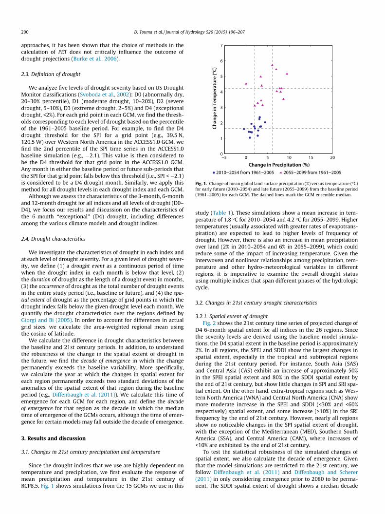
Fig. 1. Change of mean global land surface precipitation (%) versus temperature (�C)for early future (2010–2054) and late future (2055–2099) from the baseline period(1961–2005) for each GCM. The dashed lines mark the GCM ensemble median.

200 D. Touma et al. / Journal of Hydrology 526 (2015) 196–207

approaches, it has been shown that the choice of methods in thecalculation of PET does not critically influence the outcome ofdrought projections (Burke et al., 2006).

2.3. Definition of drought

We analyze five levels of drought severity based on US DroughtMonitor classifications (Svoboda et al., 2002): D0 (abnormally dry,20–30% percentile), D1 (moderate drought, 10–20%), D2 (severedrought, 5–10%), D3 (extreme drought, 2–5%) and D4 (exceptionaldrought, <2%). For each grid point in each GCM, we find the thresh-olds corresponding to each level of drought based on the percentileof the 1961–2005 baseline period. For example, to find the D4drought threshold for the SPI for a grid point (e.g., 39.5 N,120.5 W) over Western North America in the ACCESS1.0 GCM, wefind the 2nd percentile of the SPI time series in the ACCESS1.0baseline simulation (e.g., �2.1). This value is then considered tobe the D4 threshold for that grid point in the ACCESS1.0 GCM.Any month in either the baseline period or future sub-periods thatthe SPI for that grid point falls below this threshold (i.e., SPI < �2.1)is considered to be a D4 drought month. Similarly, we apply thismethod for all drought levels in each drought index and each GCM.

Although we assess the characteristics of the 3-month, 6-monthand 12-month drought for all indices and all levels of drought (D0–D4), we focus our results and discussion on the characteristics ofthe 6-month ‘‘exceptional’’ (D4) drought, including differencesamong the various climate models and drought indices.

2.4. Drought characteristics

We investigate the characteristics of drought in each index andat each level of drought severity. For a given level of drought sever-ity, we define (1) a drought event as a continuous period of timewhen the drought index in each month is below that level, (2)the duration of drought as the length of a drought event in months,(3) the occurrence of drought as the total number of drought eventsin the entire study period (i.e., baseline or future), and (4) the spa-tial extent of drought as the percentage of grid points in which thedrought index falls below the given drought level each month. Wequantify the drought characteristics over the regions defined byGiorgi and Bi (2005). In order to account for differences in actualgrid sizes, we calculate the area-weighted regional mean usingthe cosine of latitude.

We calculate the difference in drought characteristics betweenthe baseline and 21st century periods. In addition, to understandthe robustness of the change in the spatial extent of drought inthe future, we find the decade of emergence in which the changepermanently exceeds the baseline variability. More specifically,we calculate the year at which the changes in spatial extent foreach region permanently exceeds two standard deviations of theanomalies of the spatial extent of that region during the baselineperiod (e.g., Diffenbaugh et al. (2011)). We calculate this time ofemergence for each GCM for each region, and define the decadeof emergence for that region as the decade in which the mediantime of emergence of the GCMs occurs, although the time of emer-gence for certain models may fall outside the decade of emergence.

3. Results and discussion

3.1. Changes in 21st century precipitation and temperature

Since the drought indices that we use are highly dependent ontemperature and precipitation, we first evaluate the response ofmean precipitation and temperature in the 21st century ofRCP8.5. Fig. 1 shows simulations from the 15 GCMs we use in this

study (Table 1). These simulations show a mean increase in tem-perature of 1.8 �C for 2010–2054 and 4.2 �C for 2055–2099. Highertemperatures (usually associated with greater rates of evapotrans-piration) are expected to lead to higher levels of frequency ofdrought. However, there is also an increase in mean precipitationover land (2% in 2010–2054 and 6% in 2055–2099), which couldreduce some of the impact of increasing temperature. Given theinterwoven and nonlinear relationships among precipitation, tem-perature and other hydro-meteorological variables in differentregions, it is imperative to examine the overall drought statususing multiple indices that span different phases of the hydrologiccycle.

3.2. Changes in 21st century drought characteristics

3.2.1. Spatial extent of droughtFig. 2 shows the 21st century time series of projected change of

D4 6-month spatial extent for all indices in the 26 regions. Sincethe severity levels are derived using the baseline model simula-tions, the D4 spatial extent in the baseline period is approximately2%. In all regions, the SPEI and SDDI show the largest changes inspatial extent, especially in the tropical and subtropical regionsduring the 21st century period. For instance, South Asia (SAS)and Central Asia (CAS) exhibit an increase of approximately 50%in the SPEI spatial extent and 80% in the SDDI spatial extent bythe end of 21st century, but show little changes in SPI and SRI spa-tial extent. On the other hand, extra-tropical regions such as Wes-tern North America (WNA) and Central North America (CNA) showmore moderate increase in the SPEI and SDDI (<30% and <60%respectively) spatial extent, and some increase (>10%) in the SRIfrequency by the end of 21st century. However, nearly all regionsshow no noticeable changes in the SPI spatial extent of drought,with the exception of the Mediterranean (MED), Southern SouthAmerica (SSA), and Central America (CAM), where increases of<10% are exhibited by the end of 21st century.

To test the statistical robustness of the simulated changes ofspatial extent, we also calculate the decade of emergence. Giventhat the model simulations are restricted to the 21st century, wefollow Diffenbaugh et al. (2011) and Diffenbaugh and Scherer(2011) in only considering emergence prior to 2080 to be perma-nent. The SDDI spatial extent of drought shows a median decade

WNA CNA ENA CAM

CAS

SAS

SAH

WAF

SQF

GRL

CSA

TIB NAU

EAF

SAFSAU

EQF

ALA

SSA

MED

NAS

EAS

SEA

NEU

NEE

AMZ

0

40

SDDISPEISRISPI

ALA GRL

WNA CNAENA

CAM

AMZ

CSA

SSA

NEU NEE NAS

MED CAS TIB EAS

SAHWAF EAF

SQF

SAF

SASSEA

NAU

SAU

EQF

80

0

40

80

0

40

80

0

40

80

0

40

80

0

40

80

0

40

80

0

40

80

Ch

an

ge

of

spa

tia

l e

xte

nt

of

D4

dro

ug

ht

com

pa

red

to

th

e 1

96

1-2

00

5 b

ase

lin

e p

eri

od

(%

)

Regions defined by Giorgi and Bi (2005)

Z D A

W A

Fig. 2. Change of spatial extent of SPI, SRI, SPEI and SDDI 6-month D4 drought in the future period (2010–2099) relative to the baseline period (1961–2005). The time seriesshows the change of annual GCM ensemble mean spatial extent for each region defined by Giorgi and Bi (2005). The vertical lines mark the median decade of emergence foreach region and for each index. Missing vertical lines indicate no permanent emergence of the spatial extent of drought by 2080 for the corresponding region and index.

D. Touma et al. / Journal of Hydrology 526 (2015) 196–207 201

of emergence prior to 2080 for 15 subtropical and tropical regions,with the Sahara (SAH), East Africa (EAF) and West Africa (WAF)showing median emergence in the 2020s (Fig. 2). The SPEI spatialextent of drought shows a median decade of emergence for nineregions, with the earliest decade of emergence occurring in the2040s in WAF. On the other hand, there are no regions withchanges in spatial extent that permanently exceed two standarddeviations of the baseline variability of SPI and SRI during the21st century of RCP8.5.

3.2.2. Occurrence of drought eventsFig. 3 shows the spatial pattern of changes in the occurrences of

6-month D4 drought episodes in the early (2010–2054) and late(2055–2099) 21st century periods. Additionally, we have quanti-fied the agreement among the GCMs in the projections to addressthe uncertainty in the multi-model projections. In general, the SPIshows the least agreement and the SPEI shows the most agreementamong the GCMs. The SPI shows greater agreement among themodels over CAM, Amazon (AMZ), South Africa (SAF) and MED,

all of which exhibit greater occurrences of the D4 drought episodesin the late 21st century period. Similarly, the SRI and SPEI show lar-ger changes and greater agreement among models in the late 21stcentury period (Fig. 3b, d and f). In contrast, the SDDI showschanges occurring in different regions for each of the two futureperiods (Fig. 3g and h). For example, AMZ shows increases ofapproximately 10 SDDI drought occurrences in the 45 years ofthe early 21st century period, but no changes in the later period.Comparatively, CAS shows increases of approximately 10 SDDIdrought occurrences in the 45 years of the early 21st century per-iod, but decreases of approximately 3 occurrences in the later per-iod (Fig. 3g and h). It is important to note that these decreases inoccurrence do not necessarily imply fewer total months of drought,as the drought events could be longer in duration and thereforeshow fewer separate occurrences during the 45-year period (seeSection 3.2.3 below).

Our analysis shows that even if a region exhibits strongagreement in the sign of change among the GCMs, there couldstill be a discrepancy in the magnitude of this change, unveiling

(a) (b)

(c) (d)

(e) (f)

(g) (h)

Fig. 3. Change of 6-month D4 drought occurrence in the early future period (2010–2054) and late future period (2055–2099) relative to the baseline period (1961–2005),using (a, b) SPI, (c, d) SRI, (e, f) SPEI and (g, h) SDDI. The color shows the GCM ensemble mean. Areas with no stippling indicate where 90% or more of the GCMs agree on thesign of change, the white stippling shows where at least two-thirds of the GCMs agree on the sign of change and the grey lines show where less than two-thirds of the GCMsagree on the sign of change.

202 D. Touma et al. / Journal of Hydrology 526 (2015) 196–207

the uncertainty among the GCMs. For example, the SPEI andSDDI show strong agreement (among at least two-thirds ofGCMs) in the sign of change of D4 6-month drought occurrencesover Western and Central North America in the late 21st centuryperiod (Fig. 3f and h). However, the spread in the magnitude ofthe changes is large (Fig. 4g and h). The CNA region shows achange in SDDI occurrence ranging from an increase of 3 to 13events in 45 years and a change in SPEI occurrence ranging froma decrease of 10 events to an increase of 40 events in 45 years.On the other hand, other regions, including Central South Amer-ica (CSA) and SSA, show strong agreement in the sign of change

in SPEI and SDDI occurrence in the late 21st century period(Fig. 3f and h), and also exhibit a relatively small spread in themagnitude of change (Fig. 4g and h). Although there are differ-ences in the inter-model spread for the change in occurrencesbetween the two 21st century periods, the spread tends to begreater over most regions for the later period.

3.2.3. Duration of drought eventsFig. 5 shows the spatial pattern of changes in the duration of D4

drought episodes in the 2010–2054 and 2055–2099 periods ofRCP8.5. The mean duration of 6-month D4 drought events is still

CAS

SAS

SAHWAF

SQF

GRL

CSA

TIB

NAU

EAF

SAFSAU

EQF

ALA

SSA

MED

NAS

EAS

SEA

NEU

NEE

CAM

WNA

ENACNA

AMZ

2010-2054

1284-4 0

CAS

SAS

SAHWAF

SQF

GRL

CSA

TIB

NAU

EAF

SAFSAU

EQF

ALA

SSA

MED

NAS

EAS

SEA

NEU

NEE

CAM

WNA

ENACNA

AMZ

0 10 20 30

0 10 20 0 20 40

0 20 40 600 10 20 30-10

CAS

SAS

SAHWAF

SQF

GRL

CSA

TIB

NAU

EAF

SAFSAU

EQF

ALA

SSA

MED

NAS

EAS

SEA

NEU

NEE

CAM

WNA

ENACNA

AMZ

CAS

SAS

SAHWAF

SQF

GRL

CSA

TIB

NAU

EAF

SAFSAU

EQF

ALA

SSA

MED

NAS

EAS

SEA

NEU

NEE

CAM

WNA

ENACNA

AMZ

SPI SRI SPEI SDDI

2055-2099

a b c

e f g

change in number of events/45 years

0 4 8

0 4 8 12-4

d

h

Fig. 4. Change of 6-month D4 drought occurrence in 2010–2054 (a–d) and 2055–2099 (e–h) relative to the baseline period (1961–2005) for each region using (a, e) SPI, (b, f)SRI, (c, g) SPEI and (d, h) SDDI. The range of the GCM ensemble is shown, where the center line in the box is the 50th percentile of the ensemble, the left and right boundariesof the box represent the 25th and 75th percentiles respectively and the red crosses show the outliers which fall approximately outside the 99th percentile in the GCMdatasets. The region definitions are from Giorgi and Bi (2005) as seen in Fig. 2.

D. Touma et al. / Journal of Hydrology 526 (2015) 196–207 203

relatively low in the 2010–2054 period (Fig. 5a, c, e and g), with theexception of SDDI, which shows long-lasting drought events inSAH and AMZ (Fig. 5g). The 2055–2099 period shows much longerSPEI and SDDI drought durations (Fig. 5f and h), where SAH andAMZ have SDDI and SPEI drought events longer than 10 and3 years, respectively. These large increases in the duration of SDDI

episodes help to explain the decreases in drought occurrence overthese regions (Section 3.2.2), as large increases in duration tend toreduce number of individual occurrences, particularly for very longduration events. In contrast, the higher latitudes tend to show rel-atively little change in drought duration, even in the 2055–2099period. Changes in drought characteristics in these higher latitude

2010-2054 2055-2099SP

ISR

ISP

EISD

DI

0

2

4

6

8

0

12

4

8

0

24

8

16

0

120

40

80

mean duration of drought event (months)

(a) (b)

(c) (d)

(g) (h)

(e) (f)

Fig. 5. GCM ensemble mean duration of a 6-month D4 drought event in 2010–2054 (a–g) and 2055–2099 (b–h) for the SPI (a, b), SRI (c, d), SPEI (e, f) and SDDI (g, h). In thebaseline period (1961–2005), the mean duration is between 1 and 2 months for all regions and all indices (not shown here).

204 D. Touma et al. / Journal of Hydrology 526 (2015) 196–207

regions can therefore be explained predominantly by changes indrought occurrence.

Fig. 6 captures the relationship between the ensemble-medianchanges in drought duration and occurrence for the 26 regions.In most of the regions, there is an increase in both the occurrenceand duration of drought. Exceptions include the SAH and WAFregions in the 2055–2099 period, where the SDDI duration ofdrought increases by more than 500 and 420 months respectively,but the occurrence of drought decreases (Fig. 6h). These largeincreases in the SDDI duration of drought can also be inferred fromthe spatial extent of drought in SAH and WAF (Fig. 2). In theseregions, the SDDI spatial extent increases and remains high, with>80% of the regions being under D4 drought throughout the2055–2099 period. The large extent of D4 drought can beexplained by the large increases in global temperature (Fig. 1) inthe 2055–2099 period in RCP8.5, (which range spatially from2 �C to 11 �C (IPCC, 2013)). which in turn explain the decreases in

the deficit (P–PET). In addition, the non-parametric standardizationof the deficit used in the calculation of the SDDI allows the SDDI todecrease continuously and rapidly throughout the 21st century,resulting in large increases in the duration of SDDI drought.

In contrast, several areas, including Eastern North America(ENA), Greenland (GRL), Alaska (ALA) and North Asia (NAS) regionsshow decreases, albeit small, in both the occurrences and durationof SPI drought events in the 2050–2099 period (Fig. 6b). In thesame period, there is also a minimal decrease in occurrences andduration of SRI events in Southeast Asia (SEA) (Fig. 6d). Moreover,in 2010–2054, the changes in the occurrence of SPEI and SDDI arelarge, while the changes in duration are small for most regions(Fig. 6e and g). On the other hand, the 2055–2099 period showslarge increases in both the occurrence and duration of SPEI andSDDI (Fig. 6f and h). The 2010–2054 period shows similar changesin SPI and SRI duration and occurrence among the regions, whilethe 2055–2099 period shows regions where the SPI and SRI

WNACNAENACAMAMZNEUMEDSAHWAFEAFEQFCASTIBEASSASNAUSAUSAFSQFSEACSASSANEENASALAGRL

−0.2 0.0 0.2 0.4 0.6 0.8

0

5

10

15

0

5

10

15

−0.2 0.0 0.2 0.4 0.6 0.8Ch

ange

in n

umbe

r of e

vent

s / 4

5 ye

ars

SPI

2010−2054 2055−2099

0.0 0.5 1.0 1.5

0

5

10

15

0.0 0.5 1.0 1.5

0

5

10

15

SRI

0 5 10 15

0

10

20

30

40

0 5 10 15

0

10

20

30

40

SPEI

Change in average duration of drought event (months)

SDDI

a b

c d

e f

g h

0

2

4

6

-2

0

2

4

6

-2

8

0 100 500200 300 4000 100 500200 300 400

Fig. 6. GCM ensemble median change in the number of drought events related to the GCM ensemble median change in the average duration of a drought event from thebaseline period (1960–2005) for 2010–2054 (a, c, e, g) and 2055–2099 (b, d, f, h) for SPI (a, b), SRI (c, d), SPEI (e, f) and SDDI (g, h) for each region. The region definitions arefrom Giorgi and Bi (2005) as seen in Fig. 2.

D. Touma et al. / Journal of Hydrology 526 (2015) 196–207 205

duration and occurrence are more responsive to the RCP 8.5 forcing(Fig. 6a–d), with the MED, AMZ, CAM and SSA being examples ofthis stronger response.

3.3. Multi-index and multi-model assessments

Our analysis shows that many regions exhibit increases in thespatial extent, duration and occurrence of drought in the 21st cen-tury of the RCP8.5 pathway. However, by using multiple GCMs andmultiple indices we also highlight the uncertainty of the responsesof the drought characteristics.

The smallest increases occur in the SPI spatial extent and dura-tion of drought (Figs. 2 and 5), even in locations where all otherindices show relatively large increases. However, there are somenoticeable increases in occurrence (Fig. 3). Areas where SPI occur-rence increases tend to correspond to decreases in the annual pre-cipitation in RCP8.5 (Diffenbaugh and Field, 2013), suggesting thatdecreases in annual precipitation over the 21st century could leadto greater SPI drought occurrence, but not necessarily greater spa-tial extent or duration.

Alternatively, stronger increases in the spatial extent, durationand occurrence are seen in SPEI and SDDI, along with greateragreement on the sign of change among the GCMs. Although these

indices take both precipitation and temperature into account, it isclear that they are highly responsive to the temperature changesthat occur in RCP8.5 (Fig. 1), with the largest increases in SPEIand SDDI drought occurrence, duration and spatial extent co-occurring with the largest increases in annual temperature (i.e.,over North and West Africa and the Mediterranean and Amazonregions) (Diffenbaugh and Field, 2013). The effect of these changesin temperature is therefore amplified in the SDDI and SPEI, whichuse temperature as the sole, non-stationary variable, as defined inthe Thornthwaite equation for PET. However, we note that whenCook et al. (2014) use the Penman–Monteith method for PET, theyalso find that PET is the main contributor to large decreases in theaverage SPEI index in 2080–2099 in RCP8.5 over most of the globe.Therefore, irrespective of PET method choice, large increases indrought are projected in the 21st century when using a deficit var-iable (P–PET).

We note a number of important caveats to our analyses. Thechanges in SRI drought characteristics in this study reflect thechanges in surface runoff and not the total runoff, as originallystudied by Shukla and Wood (2008). We can better representdrought characteristics by using the total runoff, which respondsto changes in climate variables at longer time scales, rather thanusing surface runoff, which responds to changes at shorter, more

206 D. Touma et al. / Journal of Hydrology 526 (2015) 196–207

instantaneous timescales. Therefore, the absence of sub-surfacerunoff in our analysis could potentially enhance the spread amongthe GCMs’ simulated responses and cause low agreement amongthe GCMs as seen in Figs. 3 and 4.

We also note that our study does not include a soil moistureindex, which could alter the range of responses of the droughtcharacteristics. Orlowsky and Seneviratne (2013) use the soil mois-ture anomaly to quantify drought in the CMIP5 ensemble. Similarto our study, they find large increases in drought frequency inmany regions, although the soil-moisture-based changes are smal-ler in magnitude than the changes we identify using the SPEI andSDDI.

In addition, because our drought severity categories (D0–D4)are defined relative to the baseline variability, biases in thesimulated variability could influence the results. For example,insufficient variability in the baseline period could enhance thesimulated increase in drought occurrence resulting from a givensimulated temperature trend, and show an earlier decade ofemergence.

Finally, it is important to emphasize that even in regions wherethere is strong agreement on the sign of the change in occurrencesof drought events (Fig. 3), there are still large discrepancies in themagnitude of these changes among the GCMs. This result expandson previous drought studies that also find large uncertaintiesamong GCMs when projecting drought into the 21st century usingeither the CMIP3 or the CMIP5 ensemble (Dai, 2012; Orlowsky andSeneviratne, 2013; Sheffield and Wood, 2007). In addition, uncer-tainty arising from internal variability and emissions pathway(Hawkins and Sutton, 2009) could potentially create further uncer-tainty in the drought indices. In fact, Orlowsky and Seneviratne(2013) find that although internal variability can be the mainsource of uncertainty in SPI drought projections, the spread amongthe GCMs can overwhelm both scenario uncertainty and internalvariability in shaping uncertainty in soil moisture anomaly projec-tions for the late 21st century. However, although the GCM uncer-tainties, in our study and others, can be large and variable amongindices and regions, we extend the analysis by showing thestrength of agreement (or disagreement) of the GCMs on the signof change in the occurrence of drought in the 21st century (Fig. 3).

4. Conclusions

We find that spatial extent, occurrence and duration of ‘‘excep-tional’’ (D4) drought increase in subtropical and tropical regions inall four drought indices in the 21st century of the RCP8.5 pathway.Additionally, the increases in SPEI and SDDI drought extend intothe higher latitudes, including Southern South America, SouthAfrica and Southern Australia in the southern hemisphere, andNortheastern Europe and Central North America in the northernhemisphere. In addition, we find high agreement in the sign ofthe change over many areas of the globe, including emergence ofchanges in the frequency of drought that permanently exceedtwo standard deviations of the baseline variability in multipleregions.

Our results have important implications for near- and long-term climate risk management. Given that the risk of impacts onhuman and natural systems results from the intersection of hazard,exposure and vulnerability (Oppenheimer et al., 2014), increases inthe likelihood of drought hazards implies increasing risk fordrought-sensitive systems. For regions to manage these droughtrisks, both local and inter-regional water management policies willlikely have to be modified and adapted in the coming decades, asexisting water management practices are unlikely to be able toreduce negative impacts of drought on water supply reliabilityand aquatic systems (Kundzewicz et al., 2008). In addition, global

mitigation of greenhouse gas emissions could prevent or postponethe permanent emergence of increasing drought frequency,thereby reducing the risks for humans and ecosystems.

Acknowledgements

We thank the editor, guest editor and three anonymous review-ers for their insightful and constructive comments. Support fordata storage and analysis is provided by the Oak Ridge LeadershipComputing Facility at the Oak Ridge National Laboratory, which issupported by the Office of Science of the U.S. Department of Energyunder Contract No. DE-AC05-00OR22725. We acknowledge theWorld Climate Research Program’s Working Group on CoupledModeling responsible for CMIP, and we thank the climate modelinggroups for producing and making available their CMIP5 modeloutput. We also thank U.S. Department of Energy’s Program forClimate Model Diagnosis and Intercomparison for providing coor-dinating support and leading development of software infrastruc-ture in partnership with the Global Organization for EarthSystem Science Portals for CMIP. This work at Oak Ridge NationalLaboratory is supported by Regional and Global Climate Modelingprogram of DOE Office of Science and Oak Ridge National Labora-tory LDRD project 32112413, and the work at Stanford was sup-ported in part by NSF award #0955283 to NSD.

Appendix A. Supplementary material

Supplementary data associated with this article can be found, inthe online version, at http://dx.doi.org/10.1016/j.jhydrol.2014.12.011.

References

Allen, C.D., Macalady, A.K., Chenchouni, H., Bachelet, D., McDowell, N., Vennetier,M., Kitzberger, T., Rigling, A., Breshears, D.D., Hogg, E.H., Gonzalez, P., Fensham,R., Zhang, Z., Castro, J., Demidova, N., Lim, J.-H., Allard, G., Running, S.W.,Semerci, A., Cobb, N., 2010. A global overview of drought and heat-induced treemortality reveals emerging climate change risks for forests. For. Ecol. Manage.259, 660–684. http://dx.doi.org/10.1016/j.foreco.2009.09.001.

Anderegg, L.D.L., Anderegg, W.R.L., Abatzoglou, J., Hausladen, A.M., Berry, J.A., 2013.Drought characteristics’ role in widespread aspen forest mortality acrossColorado, USA. Glob. Chang. Biol. 19, 1526–1537. http://dx.doi.org/10.1111/gcb.12146.

Andréasson, J., Bergström, S., Carlsson, B., Graham, L.P., Lindström, G., 2004.Hydrological change – climate change impact simulations for Sweden. Ambio33, 228–234.

Ashfaq, M., Bowling, L.C., Cherkauer, K., Pal, J.S., Diffenbaugh, N.S., 2010. Influence ofclimate model biases and daily-scale temperature and precipitation events onhydrological impacts assessment: A case study of the United States. J. Geophys.Res. 115, D14116. http://dx.doi.org/10.1029/2009JD012965.

Ashfaq, M., Ghosh, S., Kao, S.-C., Bowling, L.C., Mote, P., Touma, D., Rauscher, S.A.,Diffenbaugh, N.S., 2013. Near-term acceleration of hydroclimatic change in thewestern U.S. J. Geophys. Res. Atmos. 118 (10), 676–10,693. http://dx.doi.org/10.1002/jgrd.50816.

Burke, E.J., Brown, S.J., Christidis, N., 2006. Modeling the recent evolution of globaldrought and projections for the twenty-first century with the Hadley Centreclimate model. J. Hydrometeorol. 7, 1113–1126.

Chadwick, R., Boutle, I., Martin, G., 2013. Spatial patterns of precipitation change inCMIP5: Why the rich do not get richer in the tropics. J. Clim. 26, 3803–3822.http://dx.doi.org/10.1175/JCLI-D-12-00543.1.

Ciais, P., Reichstein, M., Viovy, N., Granier, A., Ogée, J., Allard, V., Aubinet, M.,Buchmann, N., Bernhofer, C., Carrara, A., Chevallier, F., De Noblet, N., Friend,A.D., Friedlingstein, P., Grünwald, T., Heinesch, B., Keronen, P., Knohl, A., Krinner,G., Loustau, D., Manca, G., Matteucci, G., Miglietta, F., Ourcival, J.M., Papale, D.,Pilegaard, K., Rambal, S., Seufert, G., Soussana, J.F., Sanz, M.J., Schulze, E.D.,Vesala, T., Valentini, R., 2005. Europe-wide reduction in primary productivitycaused by the heat and drought in 2003. Nature 437, 529–533. http://dx.doi.org/10.1038/nature03972.

Cook, B.I., Smerdon, J.E., Seager, R., Coats, S., 2014. Global warming and 21st centurydrying. Clim. Dyn. http://dx.doi.org/10.1007/s00382-014-2075-y.

Dai, A., 2011. Drought under global warming: a review. Wiley Interdiscip. Rev. Clim.Chang. 2, 45–65. http://dx.doi.org/10.1002/wcc.81.

Dai, A., 2012. Increasing drought under global warming in observations and models.Nat. Clim. Chang. 3, 52–58. http://dx.doi.org/10.1038/nclimate1633.

D. Touma et al. / Journal of Hydrology 526 (2015) 196–207 207

Diffenbaugh, N.S., Ashfaq, M., Scherer, M., 2011. Transient regional climate change:analysis of the summer climate response in a high-resolution, century-scale,ensemble experiment over the continental United States. J. Geophys. Res. 116,1–16. http://dx.doi.org/10.1029/2011JD016458.

Diffenbaugh, N.S., Field, C.B., 2013. Changes in ecologically critical terrestrialclimate conditions. Science 341, 486–492. http://dx.doi.org/10.1126/science.1237123.

Diffenbaugh, N.S., Scherer, M., 2011. Observational and model evidence ofglobal emergence of permanent, unprecedented heat in the 20th and 21stcenturies. Clim. Change 107, 615–624. http://dx.doi.org/10.1007/s10584-011-0112-y.

Epule, T.E., Peng, C., Lepage, L., 2014. Environmental refugees in sub-Saharan Africa:a review of perspectives on the trends, causes, challenges and way forward.GeoJournal 343, 1–14. http://dx.doi.org/10.1007/s10708-014-9528-z.

Fujihara, Y., Tanaka, K., Watanabe, T., Nagano, T., Kojiri, T., 2008. Assessing theimpacts of climate change on the water resources of the Seyhan River Basin inTurkey: Use of dynamically downscaled data for hydrologic simulations. J.Hydrol. 353, 33–48. http://dx.doi.org/10.1016/j.jhydrol.2008.01.024.

Gemenne, F., 2011. Climate-induced population displacements in a 4 �C+ world.Philos. Trans. A. Math. Phys. Eng. Sci. 369, 182–195. http://dx.doi.org/10.1098/rsta.2010.0287.

Giorgi, F., Bi, X., 2005. Updated regional precipitation and temperature changes forthe 21st century from ensembles of recent AOGCM simulations. Geophys. Res.Lett. 32, L21715. http://dx.doi.org/10.1029/2005GL024288.

Guha-Sapir, D., Hargitt, D., Hoyois, P., 2004. Thirty Years of Natural Disasters 1974-2003: The Numbers. Presses universitaires de Louvain, Louvain-la-Neuve,Belgium.

Guttman, N., 1998. Comparing the palmer drought index and the standardizedprecipitation index. J. Am. Water Resour. Assoc. 34.

Hawkins, E., Anderson, B., Diffenbaugh, N., Mahlstein, I., Betts, R., Hegerl, G., Joshi,M., Knutti, R., McNeall, D., Solomon, S., Sutton, R., Syktus, J., Vecchi, G., 2014.Uncertainties in the timing of unprecedented climates. Nature 511. http://dx.doi.org/10.1038/nature13523, E3–5.

Hawkins, E., Sutton, R., 2009. The potential to narrow uncertainty in regionalclimate predictions. Bull. Am. Meteorol. Soc. 90, 1095–1107. http://dx.doi.org/10.1175/2009BAMS2607.1.

Hoerling, M., Schubert, S., Mo, K.C., 2013. An Interpretation of the Origins of the2012 Central Great Plains Drought Assessment Report.

Hsiang, S.M., Burke, M., Miguel, E., 2013. Quantifying the influence of climate onhuman conflict. Science 341, 1235367. http://dx.doi.org/10.1126/science.1235367.

IPCC, 2012. Managing the risks of extreme events and disasters to advance climatechange adaptation. In: Field, C.B., Barros, V., Stocker, T.F., Dahe, Q. (Eds.), ASpecial Report of Working Groups I and II of the Intergovernmental Panel onClimate Change. Cambridge University Press, Cambridge. doi: 10.1017/CBO9781139177245.

IPCC, 2013. Annex I: Atlas of global and regional climate projections. In: vanOldenborgh, G.J., Collins, M., Arblaste, J., Christensen, J.H., Marotzke, J., Power,S.B., Rummukainen, M., Zhou, T. (Eds.), Climate Change 2013: The PhysicalScience Basis. Contribution of Working Group I to the Fifth Assessment Reportof the Intergovernmental Panel on Climate Change. Cambridge University Press,Cambridge, United Kingdom and New York, NY, USA, pp. 1311–1394.

Keyantash, J., Dracup, J.A., 2002. The quantification of drought: an evaluation ofdrought indices. Bull. Am. Meteorol. Soc. 83, 1167–1180. http://dx.doi.org/10.1175/1520-0477.

Kundzewicz, Z., Mata, L., Arnell, N., Döll, P., Jimenez, B., Miller, K., Oki, T., Sen, Z.,Shiklomanov, I., 2008. The implications of projected climate change forfreshwater resources and their management 53, 3–10. http://dx.doi.org/10.1623/hysj.53.1.3.

Laio, F., 2004. Cramer–von Mises and Anderson-Darling goodness of fit tests forextreme value distributions with unknown parameters. Water Resour. Res.http://dx.doi.org/10.1029/2004WR003204.

Liu, L., Hong, Y., Looper, J., Riley, R., Yong, B., Zhang, Z., Hocker, J., Shafer, M., 2013.Climatological drought analyses and projection using SPI and PDSI : Case studyof the Arkansas Red River Basin. J. Hydrol. Eng. 18, 809–816. http://dx.doi.org/10.1061/(ASCE)HE.1943-5584.0000619.

Madadgar, S., Moradkhani, H., 2013. Drought analysis under climate change usingcopula. J. Hydrol. Eng. 18, 746–759. http://dx.doi.org/10.1061/(ASCE)HE.1943-5584.

McKee, T., Doesken, N., Kleist, J., 1993. The relationship of drought frequency andduration to time scales. Eighth Conf. Appl. Climatol.

Mishra, A.K., Singh, V.P., 2010. A review of drought concepts. J. Hydrol. 391, 202–216. http://dx.doi.org/10.1016/j.jhydrol.2010.07.012.

Mo, K.C., 2008. Model-based drought indices over the United States. J.Hydrometeorol. 9, 1212–1230. http://dx.doi.org/10.1175/2008JHM1002.1.

Myers, N., 2002. Environmental refugees: a growing phenomenon of the 21stcentury. Philos. Trans. R. Soc. Lond. B Biol. Sci. 357, 609–613. http://dx.doi.org/10.1098/rstb.2001.0953.

Nepstad, D.C., Tohver, I.M., Ray, D., Moutinho, P., Cardinot, G., 2007. Mortality oflarge trees and lianas following experimental drought in an Amazon forest.Ecology 88, 2259–2269.

Ojha, R., Kumar, D.N., Sharma, A., Mehrotra, R., 2013. Assessing severe drought andwet events over India in a future climate using a nested bias-correctionapproach. J. Hydrol. Eng. 18, 760–772. http://dx.doi.org/10.1061/(ASCE)HE.1943-5584.0000585.

Oppenheimer, M., Campos, M., Warren, R., Birkmann, J., Luber, G., O’Neill, B.,Takahashi, K., 2014. Emergent Risks and Key Vulnerabilities. In: Field, C.B.,Barros, V., Mach, K., Mastrandrea, M. (Eds.), Contribution of Working Group II tothe IPCC Fifth Assessment Report.

Orlowsky, B., Seneviratne, S.I., 2013. Elusive drought: uncertainty in observedtrends and short- and long-term CMIP5 projections. Hydrol. Earth Syst. Sci. 17,1765–1781. http://dx.doi.org/10.5194/hess-17-1765-2013.

Oubeidillah, A.A., Kao, S.-C., Ashfaq, M., Naz, B.S., Tootle, G., 2014. A large-scale,high-resolution hydrological model parameter data set for climate changeimpact assessment for the conterminous US. Hydrol. Earth Syst. Sci. 18, 67–84.http://dx.doi.org/10.5194/hess-18-67-2014.

Palmer, M.A., Lettenmaier, D.P., Poff, N.L., Postel, S.L., Richter, B.D., Warner, R., 2009.Climate change and river ecosystems: protection and adaptation options.Environ. Manage. 44, 1053–1068. http://dx.doi.org/10.1007/s00267-009-9329-1.

Phillips, O., Aragão, L., Lewis, S.L., Fisher, J., 2009. Drought sensitivity of the Amazonrainforest. Science (80-.). 323, 1344–1347. http://dx.doi.org/10.1126/science.1164033.

Poff, N.L., Allan, J.D., Bain, M.B., 1997. The natural flow regime. Bioscience 47, 769–784. http://dx.doi.org/10.2307/1313099.

Rao, A.R., Hamed, K., 2000. Flood Frequency Analysis. CRC Press, Boca Raton, FL.Rind, D., Goldberg, R., Hansen, J., Rosenzweig, C., Ruedy, R., 1990. Potential

evapotranspiration and the likelihood of future drought. J. Geophys. Res.Atmos. 95, 9983–10004. http://dx.doi.org/10.1029/JD095iD07p09983.

Rogelj, J., Meinshausen, M., Knutti, R., 2012. Global warming under old and newscenarios using IPCC climate sensitivity range estimates. Nat. Clim. Chang. 2,248–253. http://dx.doi.org/10.1038/nclimate1385.

Seth, A., Rauscher, S.A., Biasutti, M., Giannini, A., Camargo, S.J., Rojas, M., 2013.CMIP5 projected changes in the annual cycle of precipitation in monsoonregions. J. Clim. 26, 7328–7351. http://dx.doi.org/10.1175/JCLI-D-12-00726.1.

Sheffield, J., Wood, E.F., 2007. Projected changes in drought occurrence under futureglobal warming from multi-model, multi-scenario, IPCC AR4 simulations. Clim.Dyn. 31, 79–105. http://dx.doi.org/10.1007/s00382-007-0340-z.

Shukla, S., Wood, A.W., 2008. Use of a standardized runoff index for characterizinghydrologic drought. Geophys. Res. Lett. 35, 1–7. http://dx.doi.org/10.1029/2007GL032487.

Svoboda, M., LeComte, D., Hayes, M., Heim, R., Gleason, K., Angel, J., Rippey, B.,Tinker, R., Palecki, M., Stooksbury, D., Miskus, D., Stephens, S., 2002. The droughtmonitor. Bull. Am. Meteorol. Soc. 83, 1181–1190.

Taylor, K.E., Stouffer, R.J., Meehl, G.A., 2012. An overview of CMIP5 and theexperiment design. Bull. Am. Meteorol. Soc. 93, 485–498. http://dx.doi.org/10.1175/BAMS-D-11-00094.1.

Thornthwaite, C., 1948. An approach toward a rational classification of climate.Geogr. Rev. 38, 55–94.

Trenberth, K.E., Dai, A., Van Der Schrier, G., Jones, P.D., Barichivich, J., Briffa, K.R.,Sheffield, J., 2014. Global warming and changes in drought. Nat. Clim. Chang. 4,17–22. http://dx.doi.org/10.1038/NCLIMATE2067.

Van Huijgevoort, M.H.J., van Lanen, H.A.J., Teuling, A.J., Uijlenhoet, R., 2014.Identification of changes in hydrological drought characteristics from a multi-GCM driven ensemble constrained by observed discharge. J. Hydrol. 512, 421–434. http://dx.doi.org/10.1016/j.jhydrol.2014.02.060.

Vicente-Serrano, S.M., Beguería, S., López-Moreno, J.I., 2010. A multiscalar droughtindex sensitive to global warming: the standardized precipitationevapotranspiration index. J. Clim. 23, 1696–1718. http://dx.doi.org/10.1175/2009JCLI2909.1.

Wang, L., Chen, W., 2014. A CMIP5 multimodel projection of future temperature,precipitation, and climatological drought in China. Int. J. Climatol. 34, 2059–2078. http://dx.doi.org/10.1002/joc.3822.

Wang, T., Hamann, A., Spittlehouse, D.L., Aitken, S.N., 2006. Development of scale-free climate data for Western Canada for use in resource management. Int. J.Climatol. 26, 383–397. http://dx.doi.org/10.1002/joc.1247.

Wuebbles, D., Meehl, G.A., Hayhoe, K., Karl, T.R., Kunkel, K., Santer, B., Wehner, M.,Colle, B., Fischer, E.M., Fu, R., Goodman, A., Janssen, E., Kharin, V., Lee, H., Li, W.,Long, L.N., Olsen, S.C., Pan, Z., Seth, A., Sheffield, J., Sun, L., 2013. CMIP5 ClimateModel Analyses: Climate Extremes in the United States. Bull. Am. Meteorol. Soc.http://dx.doi.org/10.1175/BAMS-D-12-00172.1.

Zektser, S., Loaiciga, H.A., Wolf, J.T., 2004. Environmental impacts of groundwateroverdraft: selected case studies in the southwestern United States. Environ.Geol. 47, 396–404. http://dx.doi.org/10.1007/s00254-004-1164-3.