assessing vegetative drought from multi-temporal ndvi images · 2012-03-29 · assessing vegetative...
TRANSCRIPT
Assessing vegetative drought frommulti-temporal NDVI images
Coco Gratia Musaningabe
PhD dissertation committee
Chairprof. dr. ir. A. Veldkamp University of Twente
Promotorprof. dr. ir. A. Stein University of Twente
Assistant promotordr. ir. W. Bijker University of Twente
Membersdr. ir. J.G.P.W. Clevers Wageningen Universityprof. dr. ir. M-J. Kraak University of Twenteprof. dr. ing. P.Y. Georgiadou University of Twenteprof. dr. ir. P.H. Verburg Vrije Universiteit Amsterdam
ITC dissertation number 204ITC, P.O. Box 217, 7500 AE Enschede, The Netherlands
ISBN: 978–90–6164–329–6Printed by: ITC printing department, Enschede, The Netherlands
© Coco Gratia Musaningabe, Enschede, The NetherlandsAll rights reserved. No part of this publication may be reproduced without theprior written permission of the author.
ASSESSING VEGETATIVE DROUGHT FROMMULTI-TEMPORAL NDVI IMAGES
D I S S E R T A T I O N
to obtainthe degree of doctor at the University of Twente,
on the authority of the rector magnificus,prof. dr. H. Brinksma,
on account of the decision of the graduation committee,to be publicly defended
on Wednesday, April 18, 2012 at 16.45
by
Coco Gratia Musaningabeborn on February 9, 1979
in Kinshasa, Democratic Republic of Congo

This dissertation is approved by:
prof. dr. ir. A. Stein (promotor)dr. ir. W. Bijker (assistant promotor)
Summary
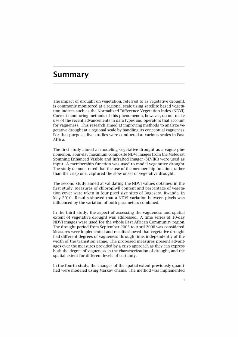
The impact of drought on vegetation, referred to as vegetative drought,is commonly monitored at a regional scale using satellite based vegeta-tion indices such as the Normalized Difference Vegetation Index (NDVI).Current monitoring methods of this phenomenon, however, do not makeuse of the recent advancements in data types and operators that accountfor vagueness. This research aimed at improving methods to analyze ve-getative drought at a regional scale by handling its conceptual vagueness.For that purpose, five studies were conducted at various scales in EastAfrica.
The first study aimed at modeling vegetative drought as a vague phe-nomenon. Four-day maximum composite NDVI images from the MeteosatSpinning Enhanced Visible and InfraRed Imager (SEVIRI) were used asinput. A membership function was used to model vegetative drought.The study demonstrated that the use of the membership function, ratherthan the crisp one, captured the slow onset of vegetative drought.
The second study aimed at validating the NDVI values obtained in thefirst study. Measures of chlorophyll content and percentage of vegeta-tion cover were taken in four pixel-size sites of Bugesera, Rwanda, inMay 2010. Results showed that a NDVI variation between pixels wasinfluenced by the variation of both parameters combined.
In the third study, the aspect of assessing the vagueness and spatialextent of vegetative drought was addressed. A time series of 10-dayNDVI images were used for the whole East African Community region.The drought period from September 2005 to April 2006 was considered.Measures were implemented and results showed that vegetative droughthad different degrees of vagueness through time, independently of thewidth of the transition range. The proposed measures present advant-ages over the measures provided by a crisp approach as they can expressboth the degree of vagueness in the characterization of drought, and thespatial extent for different levels of certainty.
In the fourth study, the changes of the spatial extent previously quanti-fied were modeled using Markov chains. The method was implemented
i
Summary
using data from 1998 to 2008, for the two main rainy seasons. Threeclasses were defined and probability transition matrices were calculated.Results showed that Markov chains offer potentials to model the dynam-ics of the spatial extent of vegetative drought at a regional scale.
The fifth study proposed a method to improve the spatio-temporal ana-lysis of vegetative drought by assessing its movement in space and timeusing an object-oriented approach. Vegetative drought and rainfall defi-cit objects were extracted and tracked. The objects were plotted in thespace-time cube. Their speed, direction and relationships were assessed.This study further quantified the spatio-temporal relationship that exis-ted between the two types of events.
This PhD research offered a quantitative approach to analyze the dy-namics of vegetative drought as a vague phenomenon at a regionalscale. Results showed that this approach provided new qualitative andquantitative information about vegetative drought that improved ourunderstanding of the phenomenon.
ii
Samenvatting
Het effect van droogte op vegetatie, of “vegetatie droogte”, wordt ge-woonlijk gemonitord op een regionale schaal. Daarbij maakt men gebruikvan vegetatie indices die gebaseerd zijn op satellietgegevens, zoals deNormalized Difference Vegetation Index (NDVI). Actuele monitoring meth-odes van vegetatie droogte maken echter nog geen gebruik van recentontwikkelde data types en operatoren, die rekening houden met vaagheid.Dit onderzoek richtte zich op het verbeteren van regionale analyse meth-odes voor vegetatie droogte, door rekening te houden met de conceptuelevaagheid. Met dat doel werden in Oost-Afrika vijf studies uitgevoerd opverschillende ruimtelijke schalen.
De eerste studie richtte zich op het modelleren van vegetatie droogteals een vaag fenomeen. Gegevens kwamen van de Meteosat SpinningEnhanced Visible and InfraRed Imager (SEVIRI) sensor. Hieruit werdenbeelden samengesteld met de maximale NDVI waarde per pixel, gemetenover vier dagen. Een lidmaatschapsfunctie werd gebruikt om vegetatiedroogte te modelleren. De studie toonde aan dat het gebruik van eenlidmaatschapsfunctie het langzaam opkomen van de vegetatie droogtebeter weergeeft dan een functie met scherpe grenzen.
De tweede studie richtte zich op het valideren van de NDVI gegevensverkregen in de eerste studie. Het chlorofyl gehalte en de percentagesvegetatie bedekking werden gemeten in mei 2010 in Bugesera, Rwanda, invier gebieden ter grootte van een pixel. De resultaten laten zien dat NDVIvariatie tussen pixels wordt beïnvloed door de gecombineerde variatievan beide parameters.
In de derde studie werd het aspect van vaagheid en de oppervlakte vanvegetatie droogte nader bestudeerd. Een tijdserie van samengesteldebeelden van de tiendaagse maximum NDVI werd gebruikt voor de heleregio van de Oost-Afrikaanse Gemeenschap (East African Community -EAC), gedurende de periode van droogte tussen september 2005 en april2006. Nieuw ontwikkelde indices werden toegepast en de resultatentoonden aan dat vegetatie droogte een verschillende mate van vaagheidkent door de tijd, onafhankelijk van de breedte van de overgangszone.In vergelijking met indices die uitgaan van scherpe grenzen hebben de
iii
Summary
voorgestelde indices het voordeel dat ze zowel de mate van vaagheid inde karakterisering van droogte als de oppervlakte van de droogte voorverschillende niveaus van zekerheid kunnen beschrijven.
In de vierde studie werden de veranderingen in de eerder gekarakter-iseerde oppervlakte gemodelleerd met gebruik van Markov reeksen. Demethode werd toegepast op gegevens van 1998 tot 2008, voor de tweebelangrijkste regenseizoenen. Drie klassen werden gedefinieerd en dematrices met de waarschijnlijkheden van de overgangen tussen dezeklassen werden berekend. De resultaten laten zien dat Markov reeksenmogelijkheden bieden om de dynamiek van de oppervlakte van vegetatiedroogte te modelleren op een regionale schaal.
In de vijfde studie werd een methode voorgesteld om de beweging vanvegetatie droogte in ruimte en tijd te beschrijven met behulp van eenobjectgerichte benadering en zo de analyse van vegetatie droogte inruimte en tijd te verbeteren. Vegetatie droogte en neerslagtekort objec-ten werden geëxtraheerd en gevolgd. De objecten werden uitgezet in eenruimte-tijd kubus. Hun snelheid, richting en onderlinge relaties werdenvastgesteld. Deze studie kwantificeerde ook de bestaande relatie tussenvegetatie droogte en neerslagtekort in ruimte en tijd.
Dit PhD onderzoek bood een kwantitatieve benadering voor de regionaleanalyse van de dynamiek van vegetatie droogte als een vaag fenomeen.De resultaten laten zien dat deze benadering nieuwe kwalitatieve enkwantitatieve informatie oplevert over vegetatie droogte, die ons begripvan het fenomeen heeft verbeterd.
iv
To my parents M. Karera and prof. dr. ir. J-B. Rulinda; andto all my siblings.

Acknowledgements
My first and foremost gratitude is expressed to my promoter, prof. dr.ir. Alfred Stein, who has been a true inspiration throughout my researchperiod. He taught me to think in the most critical and independent ways,and gain confidence in many, if not all aspects of scientific matters. Hefurther adapted to my not advisable “communication frequency” (whichmeans composed of rather long periods of silence), without loosing hispatience. It was an honour to work with him.
I extend my gratitude to my co-promoter, dr. ir. Wietske Bijker, who hasalways been professional and friendly throughout my research period inThe Netherlands and Rwanda. She will remain a role model for me. Herstrong sense of practicality and critical thinking helped me, particularlyat times of “brain freezing” events. I will always remember our lunchtrips to Intratuin or the ginger pies she was bringing, which were hertreats to help me relaxing.
I sincerely express my deepest gratitude to dr. ir. Arta Dilo, dr. ir. UlanTurdukulov, and Siqi Ding, for the inspiration and enthousiam duringour collaborative work. Many thanks to the staff of the Earth ObservationScience department and various PhD students at ITC for valuable dicus-sions and feedback; to Bas Restios and Petra Budde for their technicalsupport; to Sjoerd for the cover design; to dr. ir. Rolf de By for the LATEXthesis template design; to Teresa, Loes and all ITC support departments.
To all my friends in the Netherlands and all over the World: you havebrought support, laughter, care and love; you have put up with me inmany touching ways. I cannot mention names, neither express enoughmy gratitude. Particular thanks to IPC board members and ITC Run4funrunners with coach Wan Bakx for the memorable time we shared.
Many thanks to the Rwandan Meteorological Service for the provision ofmeteorological data and to local authorities of the disctrict of Bugeserafor facilitating the field work. Last but not least, deepest gratitude todr. Michèle A. Schilling; NUFFIC via the NPT/RWA/071 project and theNational University of Rwanda (NUR) for making this journey possible.
vii
Table of Contents
Summary i
Nomenclature xvii
1 Introduction 11.1 Motivation: drought in East Africa . . . . . . . . . . . . . . . . 21.2 Research concepts . . . . . . . . . . . . . . . . . . . . . . . . . . 31.3 Application . . . . . . . . . . . . . . . . . . . . . . . . . . . . . . 101.4 Research objectives . . . . . . . . . . . . . . . . . . . . . . . . . 111.5 Dissertation outline . . . . . . . . . . . . . . . . . . . . . . . . . 12
2 Modeling vegetative drought and vagueness using NDVI data 152.1 Introduction and background . . . . . . . . . . . . . . . . . . . 172.2 Study area and period . . . . . . . . . . . . . . . . . . . . . . . 192.3 Data acquisition and processing . . . . . . . . . . . . . . . . . 212.4 Experimental results . . . . . . . . . . . . . . . . . . . . . . . . 242.5 Sensitivity analysis . . . . . . . . . . . . . . . . . . . . . . . . . 252.6 Discussion and Conclusion . . . . . . . . . . . . . . . . . . . . 27
3 Validating MSG-SEVIRI NDVI values in East Africa 313.1 Introduction . . . . . . . . . . . . . . . . . . . . . . . . . . . . . 333.2 Data set and Study site . . . . . . . . . . . . . . . . . . . . . . . 333.3 Methods . . . . . . . . . . . . . . . . . . . . . . . . . . . . . . . . 353.4 Results and discussion . . . . . . . . . . . . . . . . . . . . . . . 383.5 Conclusion . . . . . . . . . . . . . . . . . . . . . . . . . . . . . . 43
4 Quantifying spatial extent and vagueness of vegetative drought 454.1 Introduction . . . . . . . . . . . . . . . . . . . . . . . . . . . . . 474.2 Previous work . . . . . . . . . . . . . . . . . . . . . . . . . . . . 484.3 Study area and Data . . . . . . . . . . . . . . . . . . . . . . . . 494.4 Methodology . . . . . . . . . . . . . . . . . . . . . . . . . . . . . 504.5 Results and discussion . . . . . . . . . . . . . . . . . . . . . . . 554.6 Conclusion . . . . . . . . . . . . . . . . . . . . . . . . . . . . . . 60
5 Modelling the dynamics of vegetative drought area 655.1 Introduction . . . . . . . . . . . . . . . . . . . . . . . . . . . . . 67
viii
Table of Contents
5.2 Data and study area . . . . . . . . . . . . . . . . . . . . . . . . . 695.3 Methods . . . . . . . . . . . . . . . . . . . . . . . . . . . . . . . . 705.4 Results . . . . . . . . . . . . . . . . . . . . . . . . . . . . . . . . . 765.5 Discussion . . . . . . . . . . . . . . . . . . . . . . . . . . . . . . 815.6 Conclusion . . . . . . . . . . . . . . . . . . . . . . . . . . . . . . 89
6 Assessing the spatiotemporal movement of vegetative drought 916.1 Introduction . . . . . . . . . . . . . . . . . . . . . . . . . . . . . 936.2 Materials and Methods . . . . . . . . . . . . . . . . . . . . . . . 946.3 Results . . . . . . . . . . . . . . . . . . . . . . . . . . . . . . . . . 1006.4 Discussion . . . . . . . . . . . . . . . . . . . . . . . . . . . . . . 1066.5 Conclusion . . . . . . . . . . . . . . . . . . . . . . . . . . . . . . 108
7 Synthesis 1197.1 Conclusions . . . . . . . . . . . . . . . . . . . . . . . . . . . . . . 1207.2 Reflection . . . . . . . . . . . . . . . . . . . . . . . . . . . . . . . 124
Appendices 127
A Appendix to Chapter 6 127
Bibliography 137
ix

List of Figures
1.1 Drying beans in Bugesera, Rwanda . . . . . . . . . . . . . . . . . 31.2 Percentage of reported people killed and affected by disaster
type in Rwanda . . . . . . . . . . . . . . . . . . . . . . . . . . . . . . 41.3 Vagueness in a conceptual model of spatial data uncertainty . 51.4 An illustration of concepts of internal and external data quality 61.5 Sequence of operational droughts . . . . . . . . . . . . . . . . . . 81.6 Study area: East Africa . . . . . . . . . . . . . . . . . . . . . . . . . 10
2.1 Study sites in Kenya and Rwanda . . . . . . . . . . . . . . . . . . 202.2 Drought membership function d(x) applied to DV values. . . . 242.3 Diurnal variation of NDVI on July 1, 2005 at L1, L2 and L3 . . . 252.4 (a) Drought membership values, (b) Rainfall anomaly Embu, (c)
Rainfall anomaly Kigali . . . . . . . . . . . . . . . . . . . . . . . . . 26
3.1 Bugesera district (dark grey highlighted) in the Eastern provinceof Rwanda. . . . . . . . . . . . . . . . . . . . . . . . . . . . . . . . . 34
3.2 Study sites in Bugesera, Rwanda . . . . . . . . . . . . . . . . . . . 363.3 Process of generating SEVIRI - NDVI maps per grid. . . . . . . . 383.4 Semi-variograms for chlorophyll content in grids 1, 2, 3 and 4
with a lag size of 400. . . . . . . . . . . . . . . . . . . . . . . . . . 393.5 Mean chlorophyll content values for every grid, labeled 1 to 4
in the x-axis. . . . . . . . . . . . . . . . . . . . . . . . . . . . . . . . 403.6 Mean percent vegetation cover for every grid, labeled 1 to 4 in
the x-axis. . . . . . . . . . . . . . . . . . . . . . . . . . . . . . . . . . 413.7 Variation of the daily NDVI maxima for all grids in Bugesera
(Rwanda), from 5th to 21st of May 2010 . . . . . . . . . . . . . . 423.8 Maximum and Mean NDVI, calculated for the whole period of
observation, for every grid in Bugesera, Rwanda. . . . . . . . . . 423.9 Mean Chlorophyll, Mean percentage of vegetation cover, and
Maximum NDVI, calculated for the whole period of observation,multiplied by 100, for every grid . . . . . . . . . . . . . . . . . . . 43
3.10 NDVI values multiplied by 100 and average weighted chloro-phyll percentage plotted for the four grids. . . . . . . . . . . . . 44
4.1 Vegetative drought membership functions applied to DV(t,s)images . . . . . . . . . . . . . . . . . . . . . . . . . . . . . . . . . . . 53
xi
List of Figures
4.2 A subset of vague vegetative drought maps from September2005 to April 2006 . . . . . . . . . . . . . . . . . . . . . . . . . . . 56
4.3 Averaged monthly rainfall anomaly (September 2005 - April2006) for Kenya and Tanzania . . . . . . . . . . . . . . . . . . . . 57
4.4 Total-area, core-area and mean-area of vegetative drought . . . 624.5 Vagueness of vegetative drought . . . . . . . . . . . . . . . . . . . 634.6 mean-area and cris-area of vegetative drought . . . . . . . . . . 644.7 Trajectories of vegetative drought objects existing during all
the dekads . . . . . . . . . . . . . . . . . . . . . . . . . . . . . . . . 64
5.1 Linear membership functions of dry, normal and wet classes . 715.2 State transition graph between dry, normal and wet classes,
with 1st order transition matrices . . . . . . . . . . . . . . . . . . 735.3 Absolute error values for the first season of 2008, between
the predicted and actual probability values calculated with theseasonal matrices for (a) East Africa and for (b) Kenya. . . . . . 81
5.4 Absolute error values for the second season of 2008, betweenthe predicted and actual probability values calculated with theseasonal matrices for (a) East Africa and for (b) Kenya. . . . . . 82
5.5 Predicted probability values of the areas of dry, normal andwet classes for the first season, 2008, calculated with theseasonal matrices for (a) East Africa and for (b) Kenya. . . . . . 83
5.6 Predicted probability values of the areas of dry, normal andwet classes for the second season, 2008, calculated with theseasonal matrices for (a) East Africa and for (b) Kenya. . . . . . 84
5.7 Absolute error values for the first season of 2008, betweenthe predicted and actual probability values calculated with thedekadal matrices for (a) East Africa and for (b) Kenya. . . . . . 85
5.8 Absolute error values for the second season of 2008, betweenthe predicted and actual probability values calculated with thedekadal matrices for (a) East Africa and for (b) Kenya. . . . . . 86
5.9 Predicted probability values of the areas of dry, normal andwet classes for the first season, 2008, calculated with thedekadal matrices for (a) East Africa and for (b) Kenya. . . . . . 87
5.10 Predicted probability values of the areas of dry, normal andwet classes for the second season, 2008, calculated with thedekadal matrices for (a) East Africa and for (b) Kenya. . . . . . 88
6.1 Spatio-temporal dynamics of objects represented by uniquelylabelled entities E at each time t (adapted from (Samtaneyet al., 1994)). . . . . . . . . . . . . . . . . . . . . . . . . . . . . . . . 99
6.2 Vegetative drought images of East Africa from the first dekadof March to the third dekad of May 1999 . . . . . . . . . . . . . . 102
6.3 Vegetative drought images of East Africa from the first dekadof October 1999 to the third dekad of January 2000 . . . . . . 109
6.4 Cumilative RFE deficit images of East Africa from the firstdekad of January to the third dekad of May 1999 . . . . . . . . 110
xii
List of Figures
6.5 Cumilative RFE deficit images of East Africa from the firstdekad of September to the third dekad of December 1999 . . . 111
6.6 Centroids of vd objects in (a) and (c) 3D space-time cube, (b)and (d) 2D along the Y axis (South-North), for the first andsecond seasons . . . . . . . . . . . . . . . . . . . . . . . . . . . . . 112
6.7 Centroids of rd in (a) and (c) 3D space-time cube, (b) and (d) 2Dalong the Y axis (South-North), for the first and second seasons113
6.8 Trajectories of rd and vd objects seen from their Latitudecoordinates plotted for the first season 1999. . . . . . . . . . . . 114
6.9 Trajectories of rd and vd objects seen from their Longitudecoordinates plotted for the first season 1999. . . . . . . . . . . . 114
6.10 Trajectories of rd and vd objects seen from their Latitudecoordinates objects plotted for the second season 1999. . . . . 115
6.11 Trajectories of rd and vd objects seen from their Longitudecoordinates plotted for the second season 1999. . . . . . . . . . 115
6.12 Centroids of combined vd and rd objects in (a) 3D space-time cube, and (b) 2D along the Y axis (South- North), forthe first season and in (c) 3D space-time cube, and (d) 2Dalong the Y axis (South-North) for the second season. Differentcolors represent different combined objects and different sizesrepresent different intensity values of objects. . . . . . . . . . . 116
6.13 Centroids of vd objects in (a) 3D space-time cube, (c) 2D alongthe y-axis (South-North) with a search radius of 50 pixels . . . 117
xiii

List of Tables
2.1 Land cover characteristics at the sites K1,4, R1,4 and L1,3 . . . . 212.2 Fitted coefficients A and B for equation 2.4 at the different
sites, for TR = 0.1 and TR = 0.20. Included is the shift of thetime where the fitted function takes the value 0.1. . . . . . . . . 27
3.1 ANOVA test result for chlorophyll in grids 1, 2, 3 and 4 inBugesera, Rwanda. . . . . . . . . . . . . . . . . . . . . . . . . . . . . 39
3.2 ANOVA test result for the percentage of vegetation groundcover in grids 1, 2, 3 and 4 in Bugesera, Rwanda. . . . . . . . . . 41
5.1 The parameters m, a, and b for each season in East Africa inthe upper part of the table. The mean, Stdev , the lower (L) andupper (U ) 95% confidence bounds interval of the Differenceare shown in the lower part of the table. . . . . . . . . . . . . . . 77
5.2 The parameters m, α, and β for each season in Kenya in theupper part of the table. The mean, Stdev , the lower (L) andupper (U ) 95% confidence bounds interval of the Differenceare shown in the lower part of the table. . . . . . . . . . . . . . . 79
6.1 Averaged angle for directions of vd objects from the time oftheir appearance to time of their their disappearance. . . . . . 104
6.2 Averaged angle of directions of rd objects from their appear-ance to their disappearance. . . . . . . . . . . . . . . . . . . . . . 105
A.1 Characteristics of NDVI and RFE images. . . . . . . . . . . . . . . 127A.2 Threshold values per dekad used for segmenting the rd entities.128A.3 Lat/Lon coordinates of centroids of largest vd objects for each
dekad. . . . . . . . . . . . . . . . . . . . . . . . . . . . . . . . . . . . 129A.4 Distance d (in km) and angle θ in degrees between entities of
the same vd objects. . . . . . . . . . . . . . . . . . . . . . . . . . . 130A.5 Lat/Lon coordinates of centroids of largest rd objects for each
dekad, during the the first season 1999. . . . . . . . . . . . . . . 131A.6 Lat/Lon coordinates of centroids of largest rd objects for each
dekad, during the second season 1999. . . . . . . . . . . . . . . . 132A.7 Distance d (in km) and angle θ in degrees between entities of
the same rd objects for the first season 1999. . . . . . . . . . . 133
xv
List of Tables
A.8 Distance d (in km) and angle θ in degrees between entities ofthe same rd objects for the second season 1999. . . . . . . . . . 134
A.9 Distance d (in km) between entities of closest vd and rd objectsfor both seasons. . . . . . . . . . . . . . . . . . . . . . . . . . . . . 135
xvi
Nomenclature
ANOVA Analysis of VarianceAVHRR Advanced Very High Resolution RadiometerCLM CLoud MaskCRED Centre for Research on the Epidemiology of DisastersEAC East African CommunityEUMETSAT European Organization for the Exploitation of
Meteorological SatellitesGDAL Geospatial Data Abstraction LibraryFAO Food and Agriculture OrganizationFEWS(NET) Famine Early Warning System (Network)GDP Gross Domestic ProductGIMMS Global Inventory and Monitoring SystemsGIS Geographic Information SystemGPS Global Positioning SystemITC Faculty of Geo-Information Science and Earth ObservationLAI Leaf Area IndexLSWI Land Surface Water IndexMODIS Moderate Resolution Imaging SpectroradiometerMSG Meteosat Second GenerationMVC Maximum Value CompositeNASA/GFSC National Aeronautics and Space Administration
Goddard Flight Space CenterNCDC National Climatic Data CenterNDMC National Drought Mitigation CenterNDVI Normalized Difference Vegetation IndexNDWI Normalized Difference Water IndexNICHE Netherlands Initiative for Capacity development in Higher
EducationNOAA National Oceanic and Atmospheric AdministrationNPT Netherlands Programme for the Institutional Strengthening
of Post - secondary Education and Training capacityNUFFIC Netherlands Organisation for International Cooperation in
Higher EducationRDI Reclamation Drought IndexRFE Rainfall EstimateRS Remote SensingSEVIRI Spinning Enhanced Visible and InfraRed ImagerSIWSI Shortwave Infrared Water Stress IndexSPOT Satélitte Pour l’Observation de la Terre
xvii
Nomenclature
UNICEF United Nations International Children’s Emergency FundUSGS United States Geological SurveyUTC Coordinated Universal TimeUTM Universal Transverse MercatorVCI Vegetation Condition IndexVI Vegetation IndexWGS World Geodetic System
A halfway point of the S-shape functionB steepness of the S-shape functiona lower limit of the normal classb upper limit of the normal classd distance (in Km)d(x) drought membership functionn(x) normal membership functionw(w) wet membership functionα lower limit of the transition range of the vegetative
drought functionβ upper limit of the transition range of the vegetative
drought functionm mean value of DV imagesTR Transition Rangex0 truncation or thresholdθ angle between the lines defined by the locations of two
centroids and the horizontal axisdrawn by 2 centroids
λ mean absolute errorε absolute errorStev Standard deviationDV difference NDVIDR difference RFEL lower limit of the DV 95% confidence bounds intervalU upper limit of the DV 95% confidence bounds intervalcore-area area size of all certain drought locationstotal-area area size of all possible drought locationsmean-area mean area size of possible drought locationsvagueness degree of vaguenessCx Coordinate of Centroid along the x-axisCx Coordinate of Centroid along the y-axisvd vegetative drought objectrd rainfall deficit objectrd rainfall deficitvd vegetative droughtK1 to K4 Selected locations in KenyaR1 to R4 Selected locations in RwandaL1 to L4 Selected locations near Embu (Kenya)
for diurnal variation analysis of NDVI
xviii

Nomenclature
VIS 0.6 Spectral reflectance in the SEVIRI VIS 0.6 chanelVIS 0.8 Spectral reflectance in the SEVIRI VIS 0.8 chanelRED Spectral reflectance in the Red channelNIR Spectral reflectance in the Near Infrared channelEntityID Entity identifierObjectID Object identifierN number of vegetative drought classesM number of sub-samples
xix


1Introduction
1.1 Motivation: drought in East Africa 21.2 Research concepts 31.3 Application 101.4 Research objectives 111.5 Dissertation outline 12
1
1. Introduction
1.1 Motivation: drought in East Africa
Africa has a long history of drought with severe impacts on the environ-ment, economic and social sectors. The international disaster databaseof the center for research on epidemiology of disasters (CRED)1, listsdrought as one of the most severe natural disasters in many parts ofthe continent. Environmental losses resulting from damages to plantand animals lead to many economic impacts in agriculture and relatedsectors, because of the heavy reliance of these sectors on surface andgroundwater supplies. Many of the impacts identified as economic andenvironmental have social components as well, such as population migra-tion within or outside a country. The drought migrants place increasingpressure on the social infrastructure, leading to increased poverty andsocial unrest.
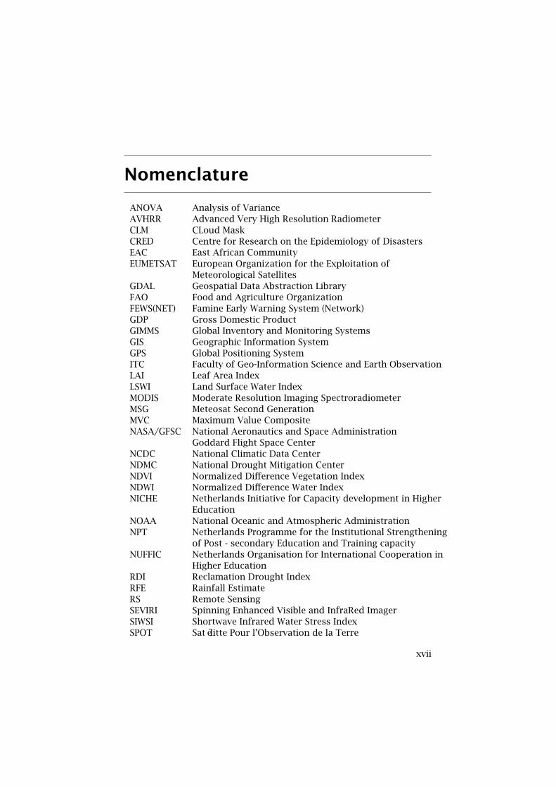
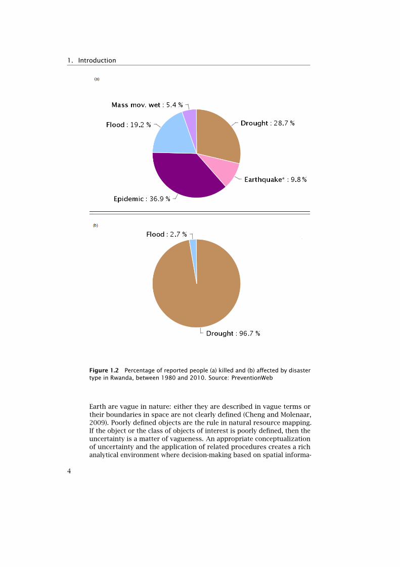
East Africa particularly is a drought prone region characterised by lowrainfall (Gommes and Petrassi, 1994). Since the late 1990s parts of EastAfrica have experienced a decline in rainfall most notably during March-April-May, the “long rain” season in many parts of the region (Bradfield,2011). As most agriculture in the region is dependent on rainfall, droughthas particularly negative impacts on agricultural production. Figure (1.1)shows drying beans in Bugesera, a drought prone region of Rwanda,during a short drought period in April 2008. Agriculture is one of theEast African region’s most important sectors, with about 80 % of thepopulation of the East African Community Partner States living in ruralareas and depending on agriculture for their livelihood (EAC, 2010). Dur-ing the last decade, media have reported many drought episodes in EastAfrica, contributing to humanitarian crises. In 2011, doctors estimatedthat admissions for severe malnutrition in children have risen by atleast 25 % in recent months. Furthermore, the United Nations indicatedthat 9 million people needed humanitarian assistance in the drought-hitcountries of the Horn of Africa. According to PreventionWeb’statistics(www.preventionweb.net), drought in Rwanda for instance has affectedand killed more than any other natural disaster, during the period from1980 to 2010 (Figure 1.2; source PreventionWeb2). The lack of food hascontributed to a surge in people leaving war-torn Somalia for neighboringKenya in search of help. Many tribes across East Africa also had to leavetheir pastoral way of life for urban poverty because of severe droughts[Andrew Wander/Save the Children].
Various national and international institutions are making efforts toreduce the negative impacts of drought in East Africa. It is in thiscontext that the Netherlands Organisation for International Cooperationin Higher Education (NUFFIC, www.nuffic.nl) sponsored this researchthrough the NPT programme. NUFFIC also supports drought related
1EM-DAT, www.emdat.be2http://www.preventionweb.net/english/countries/statistics/?cid=143
2
1.2. Research concepts
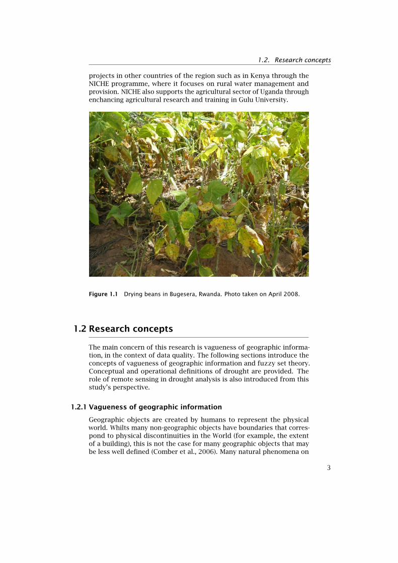
projects in other countries of the region such as in Kenya through theNICHE programme, where it focuses on rural water management andprovision. NICHE also supports the agricultural sector of Uganda throughenchancing agricultural research and training in Gulu University.
Figure 1.1 Drying beans in Bugesera, Rwanda. Photo taken on April 2008.
1.2 Research concepts
The main concern of this research is vagueness of geographic informa-tion, in the context of data quality. The following sections introduce theconcepts of vagueness of geographic information and fuzzy set theory.Conceptual and operational definitions of drought are provided. Therole of remote sensing in drought analysis is also introduced from thisstudy’s perspective.
1.2.1 Vagueness of geographic information
Geographic objects are created by humans to represent the physicalworld. Whilts many non-geographic objects have boundaries that corres-pond to physical discontinuities in the World (for example, the extentof a building), this is not the case for many geographic objects that maybe less well defined (Comber et al., 2006). Many natural phenomena on
3
1. Introduction
Figure 1.2 Percentage of reported people (a) killed and (b) affected by disastertype in Rwanda, between 1980 and 2010. Source: PreventionWeb
Earth are vague in nature: either they are described in vague terms ortheir boundaries in space are not clearly defined (Cheng and Molenaar,2009). Poorly defined objects are the rule in natural resource mapping.If the object or the class of objects of interest is poorly defined, then theuncertainty is a matter of vagueness. An appropriate conceptualizationof uncertainty and the application of related procedures creates a richanalytical environment where decision-making based on spatial informa-
4
1.2. Research concepts
tion is facilitated (Molenaar, 1998).
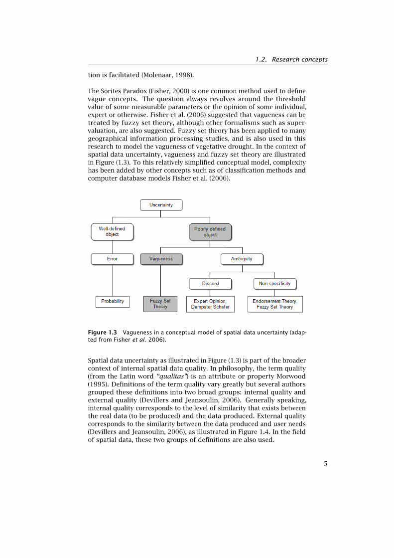
The Sorites Paradox (Fisher, 2000) is one common method used to definevague concepts. The question always revolves around the thresholdvalue of some measurable parameters or the opinion of some individual,expert or otherwise. Fisher et al. (2006) suggested that vagueness can betreated by fuzzy set theory, although other formalisms such as super-valuation, are also suggested. Fuzzy set theory has been applied to manygeographical information processing studies, and is also used in thisresearch to model the vagueness of vegetative drought. In the context ofspatial data uncertainty, vagueness and fuzzy set theory are illustratedin Figure (1.3). To this relatively simplified conceptual model, complexityhas been added by other concepts such as of classification methods andcomputer database models Fisher et al. (2006).
Figure 1.3 Vagueness in a conceptual model of spatial data uncertainty (adap-ted from Fisher et al. 2006).
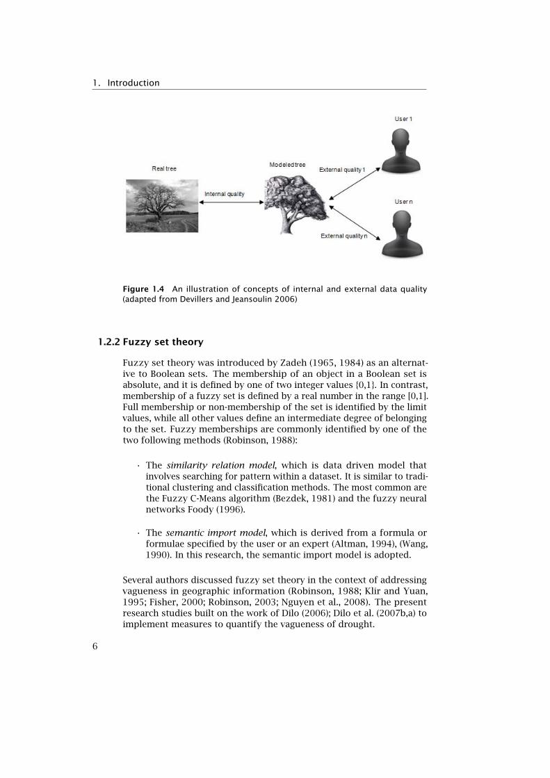
Spatial data uncertainty as illustrated in Figure (1.3) is part of the broadercontext of internal spatial data quality. In philosophy, the term quality(from the Latin word “qualitas”) is an attribute or property Morwood(1995). Definitions of the term quality vary greatly but several authorsgrouped these definitions into two broad groups: internal quality andexternal quality (Devillers and Jeansoulin, 2006). Generally speaking,internal quality corresponds to the level of similarity that exists betweenthe real data (to be produced) and the data produced. External qualitycorresponds to the similarity between the data produced and user needs(Devillers and Jeansoulin, 2006), as illustrated in Figure 1.4. In the fieldof spatial data, these two groups of definitions are also used.
5
1. Introduction
Figure 1.4 An illustration of concepts of internal and external data quality(adapted from Devillers and Jeansoulin 2006)
1.2.2 Fuzzy set theory
Fuzzy set theory was introduced by Zadeh (1965, 1984) as an alternat-ive to Boolean sets. The membership of an object in a Boolean set isabsolute, and it is defined by one of two integer values {0,1}. In contrast,membership of a fuzzy set is defined by a real number in the range [0,1].Full membership or non-membership of the set is identified by the limitvalues, while all other values define an intermediate degree of belongingto the set. Fuzzy memberships are commonly identified by one of thetwo following methods (Robinson, 1988):
• The similarity relation model, which is data driven model thatinvolves searching for pattern within a dataset. It is similar to tradi-tional clustering and classification methods. The most common arethe Fuzzy C-Means algorithm (Bezdek, 1981) and the fuzzy neuralnetworks Foody (1996).
• The semantic import model, which is derived from a formula orformulae specified by the user or an expert (Altman, 1994), (Wang,1990). In this research, the semantic import model is adopted.
Several authors discussed fuzzy set theory in the context of addressingvagueness in geographic information (Robinson, 1988; Klir and Yuan,1995; Fisher, 2000; Robinson, 2003; Nguyen et al., 2008). The presentresearch studies built on the work of Dilo (2006); Dilo et al. (2007b,a) toimplement measures to quantify the vagueness of drought.
6
1.2. Research concepts
1.2.3 Drought definitions
Drought is a weather-related recurrent feature of the climate. It occursin virtually all climatic zones, and its characteristics vary significantlyamong regions. It is related to a deficiency of precipitation over an exten-ded period of time, usually for a season or more. This deficiency resultsin a water shortage for some activity, group, or environmental sector.Drought is also related to the timing of precipitation. Other climaticfactors such as high temperature, high wind, and low relative humidityare often associated with drought. Drought differs from aridity in thatdrought is temporary; aridity is a permanent characteristic of regionswith low rainfall.
Drought is defined in two ways: (1) conceptually, and (2) operationally.Conceptual definitions help understand the meaning of drought and itseffects. Operational definitions help identify the drought’s beginning,end, and degree of severity for a given historical period. To determinethe beginning of drought, operational definitions specify the degree ofdeparture from the average over some time period. The threshold iden-tified as the beginning of a drought is usually established somewhatarbitrarily, hence characterizing the vagueness of operational droughtdefinitions.
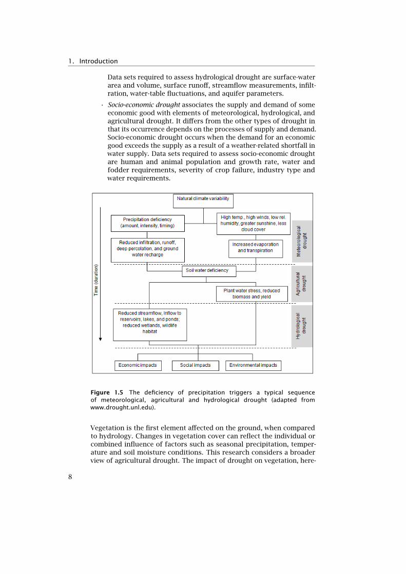
Four operational definitions of drought are commonly used, at variousscales. These occur in sequence as illustarted in Figure 1.5, and are de-scribed according to the US National Drought Mitigation Center (NDMC)as follows:
• Meteorological drought is defined on the basis of the degree of dry-ness, in comparison to a normal or average amount of precipitation,and the duration of the dry period. Definitions of meteorologicaldrought are region-specific, since the atmospheric conditions thatresult in deficiencies of precipitation are highly region-specific.Data sets required to assess meteorological drought are daily rain-fall information, temperature, humidity, wind velocity and pressure,and evaporation.
• Agricultural drought links various characteristics of meteorologicaldrought to agricultural (plant) impacts, focusing on precipitationshortages, differences between actual and potential evapotranspir-ation, soil-water deficits, reduced groundwater or reservoir levels,and so on. Plant water demand also depends on prevailing weatherconditions, biological characteristics of the specific plant, its stageof growth, and the physical and biological properties of the soil.Data sets required to assess agricultural drought are soil texture,fertility and soil moisture, crop type and area, crop water require-ments, pests and climate.
• Hydrological drought refers to a persistently low discharge and/orvolume of water in streams and reservoirs, lasting months or years.
7
1. Introduction
Data sets required to assess hydrological drought are surface-waterarea and volume, surface runoff, streamflow measurements, infilt-ration, water-table fluctuations, and aquifer parameters.
• Socio-economic drought associates the supply and demand of someeconomic good with elements of meteorological, hydrological, andagricultural drought. It differs from the other types of drought inthat its occurrence depends on the processes of supply and demand.Socio-economic drought occurs when the demand for an economicgood exceeds the supply as a result of a weather-related shortfall inwater supply. Data sets required to assess socio-economic droughtare human and animal population and growth rate, water andfodder requirements, severity of crop failure, industry type andwater requirements.
Figure 1.5 The deficiency of precipitation triggers a typical sequenceof meteorological, agricultural and hydrological drought (adapted fromwww.drought.unl.edu).
Vegetation is the first element affected on the ground, when comparedto hydrology. Changes in vegetation cover can reflect the individual orcombined influence of factors such as seasonal precipitation, temper-ature and soil moisture conditions. This research considers a broaderview of agricultural drought. The impact of drought on vegetation, here-
8
1.2. Research concepts
after called vegetative drought, can hence be characterized from thechanges of vegetation conditions in general. The definition of vegetativedrought is also vague, as transition between vegetation condition classesis gradual. Figure 1.5, presents drought in broad terms. Quantificationand uncertainties, although not represented in the figure, are present inall stages and are critical to the definition of each category of drought.To this general view of drought, the present research adds the conceptof vagueness of defining a vegetative drought.
1.2.4 Remote sensing and drought
Satellite images provide an opportunity to determine the rates of changein biotic resources in response to drought influences. Healthy, synthetic-ally active vegetation reflects near infrared light strongly, and it is mainlythis characteristic that enables the sensors to monitor the dynamics ofgreen vegetation from space. Reflectance measurements are transmittedto a ground receiving station where computers record the data. Thepresent research studies focus on processing those recorded data fordrought impact analysis on vegetation, refered to as vegetative drought.
Many studies have shown the efficiency of the use of remote sensing (RS)techniques for drought monitoring and in many regions of the world,images data are used for drought studies. The use of RS techniques tomonitor drought has been seen efficient not only in the use of droughtindices; but with the fact that remote sensing techniques offer the possib-ility to collect much information at a time, of large geographic coverage,and more frequently, with fewer resources compared to ground-basedobservations. Some regions in the world cannot afford necessary ground-based observations (terrain not accessible or resources not available) fordrought studies and as such, RS techniques provide a low cost alternativeway for collecting data. Their main advantage is their rapid and coverageof large land areas.
Drought indices are used to characterize operational droughts. Amongthem are the Percent of Normal Precipitation (PNP), the Standard Precipit-ation Index (SPI), the Deciles (monthly drought) and the Palmer DroughtSeverity Index (PDSI), developed for meteorological drought. The Sur-face Water Supply Index (SWSI) and Reclamation Drought Index (RDI)were designed to be indicators of surface water conditions and combineboth hydrological and climatological features. Vegetation indices (VI) arecommonly used to assess the impact of drought on vegetation. Amongthem are the Normalized Difference Vegetation Index (NDVI), the Veget-ation Condition Index (VCI), the Normanilzed Difference Water Index(NDWI), the Land Surface Water Index (LSWI) and Shortwave InfraredWater Stress Index (SIWSI). The NDWI, LSWI and SIWSI are more sensitiveto liquid water in plants, as compared to NDVI, and less sensitive toatmospheric scattering effects. NDWI (Gao, 1996) for instance showed
9
1. Introduction
a quicker response to drought conditions than NDVI (Gu et al., 2007,2008). These vegetation water indices are more sensitive to crop stagesand both NDWI and LSWI show strong relationships with NDVI (Gu et al.,2007; Chandrasekar et al., 2010). NDVI, although simple, has been usedsuccessfully in drought detection (Moulin et al., 1998), and furthermore,the images needed to implement our approach were available for free.For these reasons, satellite-based NDVI images are selected to illustratethe research’s approach.
1.3 Application
1.3.1 Study area
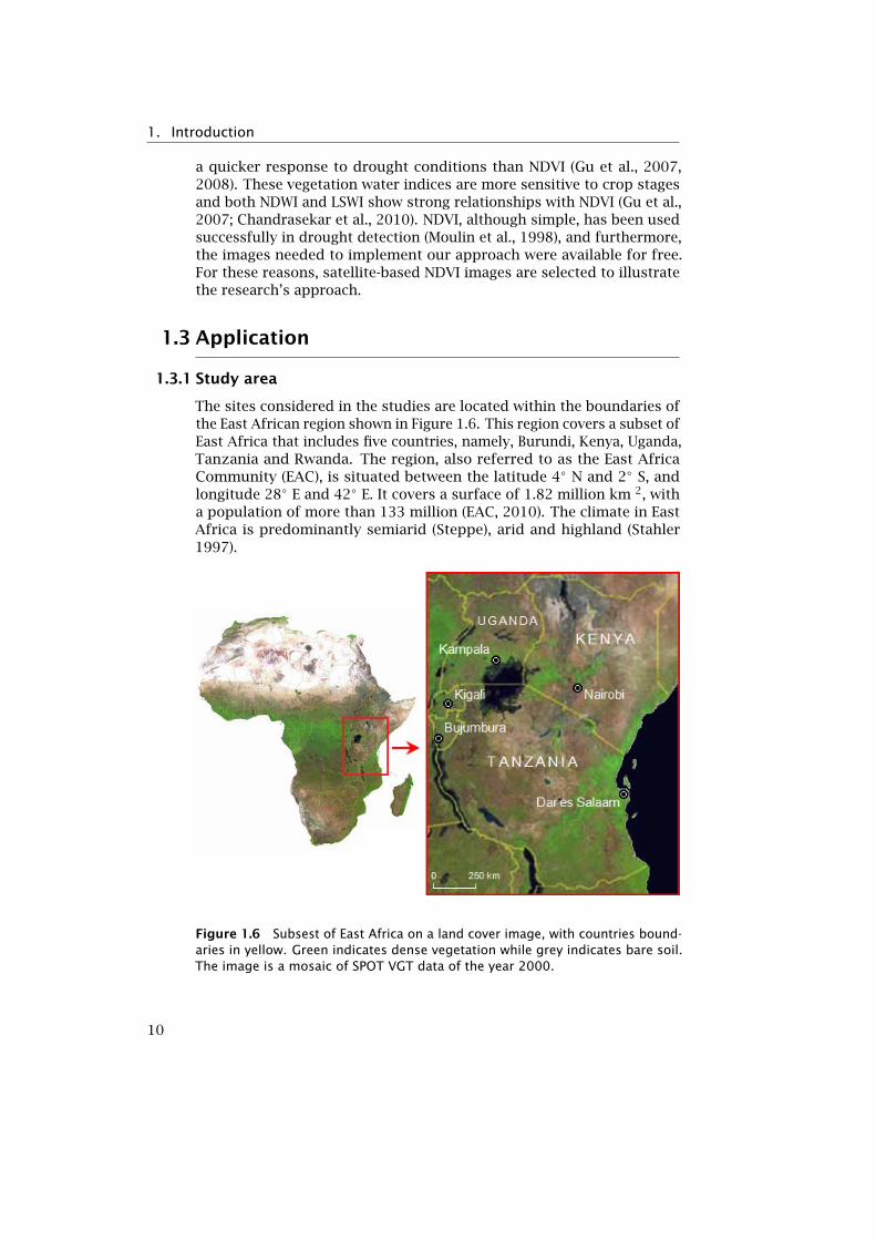
The sites considered in the studies are located within the boundaries ofthe East African region shown in Figure 1.6. This region covers a subset ofEast Africa that includes five countries, namely, Burundi, Kenya, Uganda,Tanzania and Rwanda. The region, also referred to as the East AfricaCommunity (EAC), is situated between the latitude 4◦ N and 2◦ S, andlongitude 28◦ E and 42◦ E. It covers a surface of 1.82 million km 2, witha population of more than 133 million (EAC, 2010). The climate in EastAfrica is predominantly semiarid (Steppe), arid and highland (Stahler1997).
Figure 1.6 Subsest of East Africa on a land cover image, with countries bound-aries in yellow. Green indicates dense vegetation while grey indicates bare soil.The image is a mosaic of SPOT VGT data of the year 2000.
10
1.4. Research objectives
1.3.2 Datasets description
The main dataset used in this research is the NDVI images dataset derivedfrom the National Oceanic and Atmospheric Administration - AdvancedVery High Resolution Radiometer (NOAA-AVHRR). This dataset coveringEast Africa was freely available during most of the research period atthe USGS FEWS NET Data portal 3. The NDVI images are 10-day (dekad)maximum composites, with a pixel size of 8 km. The long-term meanNDVI images are calculated for every dekad from the year 1982 to theyear 2005 at least. Detailed descriptions of the selected time periods andspatial extent are given in specific chapters.
Images from the Meteosat Second Generation - Spinning Enhanced Visibleand InfraRed Imager (MSG-SEVIRI) are also used in this research. The 15-minutes NDVI images were obtained from the first (VIS0.6, red centeredat 0.6 µm) and second (VIS0.8, near infrared centered at 0.8 µm) bands ofthe images 4. These images were imported using the EUMETCast serviceat ITC, via the MSG data retriever tool (Maathuis et al., 2005) developedfor reading the images in Geospatial Data Abstraction Library (GDAL,http://www.gdal.org). Descriptions of the selected time periods andimage characteristics are given in Chapter 2.
The NOAA-AVHRR derived Rainfall Estimate (RFE) images used as input toobtained rainfall deficit images were also imported from the same USGSFEWS NET Data portal. These data have the same spatial and temporalcharacteristics than the NDVI data. Rainfall data were also obtained forEmbu in Kenya, from the National Climatic Data Centre NCDC (2010) andrainfall data for Kigali were obtained from the Rwandan MeteorologicalService, in Kigali, Rwanda.
1.4 Research objectives
1.4.1 General objective
Metrics that allow to represent and reason with vagueness in spatialinformation within a GIS such as in Dilo et al. (2007b,a) have beendeveloped. Although vegetative drought is vague in nature, droughtmonitoring methods have not yet benefited from these advancements.As a result, the vagueness of vegetative drought is not accounted for,leaving out potential information to improve our understanding of thephenomenon.
This research aims principally at developing a methodology to modeland quantify vagueness of vegetative drought in the process of monitor-
3http://earlywarning.usgs.gov/fews/4http://www.eumetsat.int/groups/ops/documents/document/pdf_ten_052561_msg1
_spctrbnds.pdf
11
1. Introduction
ing. The proposed methodology is illustrated on monitoring vegetativedrought in East Africa at a regional level. In particular, five researchobjectives have been devised with related research questions.
1.4.2 Specific objectives
The first objective is to improve the early detection of drought usingNDVI derived Meteosat SEVIRI data in Eastern Africa. In doing so, usinga membership function to account for vagueness in the definition ofvegetative drought. The drought spell in eastern Africa at the end of theyear 2005 is used to illustrate the approach.
The second objective is to validate the observed SEVIRI NDVI values.This is performed by quantifying the spatial variability of vegetationcondition, expressed in chlorophyll content and percentage of vegetationcover. The study is implemented in Bugesera, Rwanda, on SEVIRI pixelsrelated sites. These values are then compared with SEVIRI NDVI values.
The third objective is to improve the quantification of vegetative droughtby taking into account its vagueness. Measures are proposed to quantifythe spatial extent and vagueness of vegetative drought at a regional level,using NOAA-AVHRR derived NDVI data.
The fourth objective is to model the dynamics of vegetative droughtarea. In doing so, exploring the potential of Markov chains to model ofdynamics of areas of vegetative drought at a regional scale. The methodis applied in Eastern Africa, using NOAA-AVHRR derived NDVI data.
The fifth objective is to improve the analysis of the spatio-temporalmovements of vegetative drought modeled as a vague phenomenon.In doing that, it also relates these movements to the spatio-temporalmovement of rainfall deficit. An object-oriented approach is proposedand NOAA-AVHRR derived data are used. The study is implemented inEast Africa.
1.5 Dissertation outline
This dissertation consists of seven chapters. The five core chapters (2-6)focus on the aforementioned five research objectives respectively. Thesefive chapters have either been published or are submitted for publica-tion as peer-reviewed papers in ISI journals or peer-reviewed conferencepapers.
Chapter 1 first describes the rational behind the selection of the researchtopic. The concepts used, the objectives and related research questionsare then presented. The study area and dataset are introduced and lastly,
12
1.5. Dissertation outline
the outline of the dissertation is given.
Chapter 2 addresses the first objective of the research. A method basedon fuzzy set theory is proposed to model vegetative drought and itsvagueness. The method is implemented at selected pixel-location ofvegetated sites in the Kenya and Rwanda.
Chapter 3 relates to the second objective, and describes the method usedto validate NDVI values obtained in Chapter 2. A field data collectionwas conducted in Bugesera, a drought prone-region of Rwanda, using theline transects method. The ground measurements were compared withSEVIRI derived NDVI values.
Chapter 4, related to the third objective, describes methods developedto quantify the spatial extent and vagueness of vegetative drought. Meas-ures for vague objects for continuous space proposed by Dilo (2006);Dilo et al. (2007a) are adapted for raster data.
Chapter 5, related to the fourth objective, explores the potential ofMarkov chains (Balzter, 2000) to model the dynamics of vegetativedrought classes. Markov chains have been used by various authorsto model the dynamics of random processes. In this study, it is used forthe first time to model the dynamics of vegetative drought using NDVIdata. The models are also used to predict the area of vegetative droughtclasses.
Chapter 6 is related to the fifth objective and describes the methodsused to assess the movement of vegetative drought and its relationshipwith rainfall deficit. Objects are extracted and tracked using a region-overlapping method, embedded in the Dynomap software (Turdukolov,2007). The centroids of these objects are plotted in the space-time cube.The direction and speed are further quantified.
Chapter 7 summarizes the results obtained in Chapters 2-6, discussesand conclude the studies. A reflection is provided on the main contribu-tions and limitations of these studies. Opportunities for further studiesare also discussed.
13

2Modeling vegetative drought andvagueness using NDVI data
2.1 Introduction and background 172.2 Study area and period 192.3 Data acquisition and processing 212.4 Experimental results 242.5 Sensitivity analysis 252.6 Discussion and Conclusion 27
This chapter is based on: C.M Rulinda, W. Bijker, A. Stein (2010). Imagemining for drought monitoring in Eastern Africa using Meteosat SEVIRIdata. International Journal of Applied Earth Observation and Geoinform-ation, 12 (Supp. 1), S63-S68.
15
2. Modeling vegetative drought and vagueness using NDVI data
Abstract
Meteosat Spinning Enhanced Visible and InfraRed Imager (SEVIRI) imagedata provide frequent NDVI time series which can be used to assess theevolution of drought from vegetation conditions. Vegetation conditionis characterized in space by the deviation of the current NDVI observa-tions at locations from their temporal mean values. In this study, thegradual evolution of vegetation stress is assumed caused by drought.The vagueness of vegetative drought is modeled with the use of a mem-bership function applied to vegetation stress values. The approach wasimplemented on subset image data of Eastern Africa. Vegetated sitesin a drought prone area of the region serve as an illustration using thedrought spell at the end of 2005. This study showed that the use of amembership function allows capturing the gradual evolution of droughtand can be used to model drought from observed vegetation conditions.
16
2.1. Introduction and background
2.1 Introduction and background
Drought is defined as an extended period of abnormally dry weather thatcauses water shortage and damage to vegetation. It is a creeping andrecurrent natural phenomenon and its impacts, covering large areas, canlast for weeks or months (Wilhite, 2005). The onset, duration and sever-ity of droughts are often difficult to determine and their characteristicsmay vary significantly from one region to another. In systems relyingon rainfall as the sole source of moisture for crop or pasture growth,seasonal rainfall variability is inevitably mirrored in both highly variableproduction levels as well as in the risk-averse livelihoods (Cooper et al.,2008).
Africa has a long history of rainfall fluctuations of varying lengths andintensities Nicholson (1994, 2000). At different spatial and temporalscales, studies showed different behavior of rainfall trends in Africa;while studies by Olsson et al. (2005) and Herman et al. (2005) showed anincrease of rainfall and greenness in parts of the Sahel region, Swensonand Wahr (2009) showed a decrease of water shortage in Eastern Africabetween 2003 and 2008 where drought and famine situations were peri-odically reported (FEWSNETf, 2005) (FEWSNETb, 2006).
Drought has particulary negative impacts on agricultural productionin the Eastern African region, as most of agriculture is dependent onrainfall (Barron et al., 2003), (Slegers, 2008), (Thorton et al., 2009). In thisstudy the focus is on monitoring the impacts of drought on vegetation,referred to as vegetative drought, using a membership function appliedto Meteosat Spinning Enhanced Visible and Infrared Imager (SEVIRI) data.
2.1.1 Vegetation index
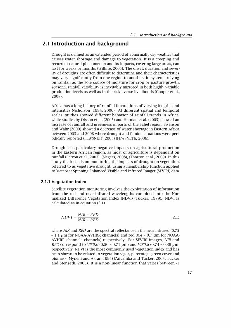
Satellite vegetation monitoring involves the exploitation of informationfrom the red and near-infrared wavelengths combined into the Nor-malized Difference Vegetation Index (NDVI) (Tucker, 1979). NDVI iscalculated as in equation (2.1)
NDVI = NIR − REDNIR + RED (2.1)
where NIR and RED are the spectral reflectance in the near infrared (0.75– 1.1 µm for NOAA-AVHRR channels) and red (0.4 – 0.7 µm for NOAA-AVHRR channels channels) respectively. For SEVIRI images, NIR andRED correspond to VIS0.6 (0.56 – 0.71 µm) and VIS0.8 (0.74 – 0.88 µm)respectively. NDVI is the most commonly used vegetation index and hasbeen shown to be related to vegetation vigor, percentage green cover andbiomass (Myneni and Asrar, 1994) (Anyamba and Tucker, 2005; Tuckerand Stenseth, 2005). It is a non-linear function that varies between -1
17
2. Modeling vegetative drought and vagueness using NDVI data
and +1, and is undefined when both NIR and RED are zero. NDVI valuesfor vegetated land areas generally range from approximately 0.1 to 0.7,with values greater than 0.5 indicating dense vegetation. Values less than0.1 indicate no vegetation but barren area, rock, sand or snow (Tucker,1979).
2.1.2 Monitoring vegetative drought
Monitoring vegetative drought usually requires a large amount of tem-poral data, and Remote Sensing (RS) technologies provide necessarymeans to collect these at regular intervals. NDVI is commonly calculatedusing image data from polar orbiting satellites, which carry sensors de-tecting radiation in red and infrared wavelengths. Despite their dailyimage data acquisitions, it may not be possible to obtain frequent cloudfree image data. In order to minimize the effects of clouds and atmo-spheric influence from aerosols and water vapor, temporal compositesof 10 or 16 days are often used (Holben, 1986). The high temporal fre-quency of SEVIRI data increases the chance to obtain cloud free imagesduring a day and daily NDVI data is now more often available (Fensholtet al., 2006).
Vegetation conditions can be characterized by the deviation of the cur-rent NDVI values from their corresponding temporal mean NDVI values,usually calculated over a long period such as one or more decades. Ateach pixel site, this deviation, referred to in this chapter as DV(t,s), iscalculated as the difference between the current NDVI value and itscorresponding time series mean (equation (2.2)) (Anyamba and Tucker,2005).
DV(t, s) = NDVI(t, s)−NDVI(s) (2.2)
where NDVI(t, s) is the current NDVI at site s and time t, and NDVI (s)is the mean NDVI value for different times, calculated for the timeframe of the data series. When DV(t,s) is negative, it indicates belownormal vegetation conditions and therefore suggests prevailing droughtconditions; a large negative, persistent in time, corresponds with a severedrought. This indicator has been used and discussed in various studies(Anyamba and Tucker, 2005) (Bajgirana et al., 2008).
2.1.3 Vegetative drought and uncertainties
Vegetation condition values, characterized by DV(t,s), are an interpret-ation of quantitative measurements of vegetation conditions. Droughtclasses are traditionally defined based on these quantitative measure-ments and modeled in geographic information systems (GIS) using tra-ditional crisp classification techniques. This approach does not reflectthe transition between the “drought” and “non-drought” classes. For
18
2.2. Study area and period
drought, a gradual transition reflecting its severity is more appropriate.Moreover, at a location, the severity of drought depends not only on theintensity of vegetation stress but also on its duration (IMWI, 2010). Sincevegetation stress caused by drought increases gradually over time, a hardspatial classification cannot discriminate potential information that canlead to a better understanding of drought onset and development. Thecoarse spatial resolution of SEVIRI data, which is 3 km at the sub-satellitepoint, introduces further spatial uncertainties due to the mixture of landcover elements.The aim of this study is to improve the early detection of drought usingMeteosat SEVIRI data in eastern Africa. In doing so, use of a membershipfunction to account for uncertainties in the definition of vegetativedrought. The drought spell in Eastern Africa at the end of the year 2005illustrates our approach.
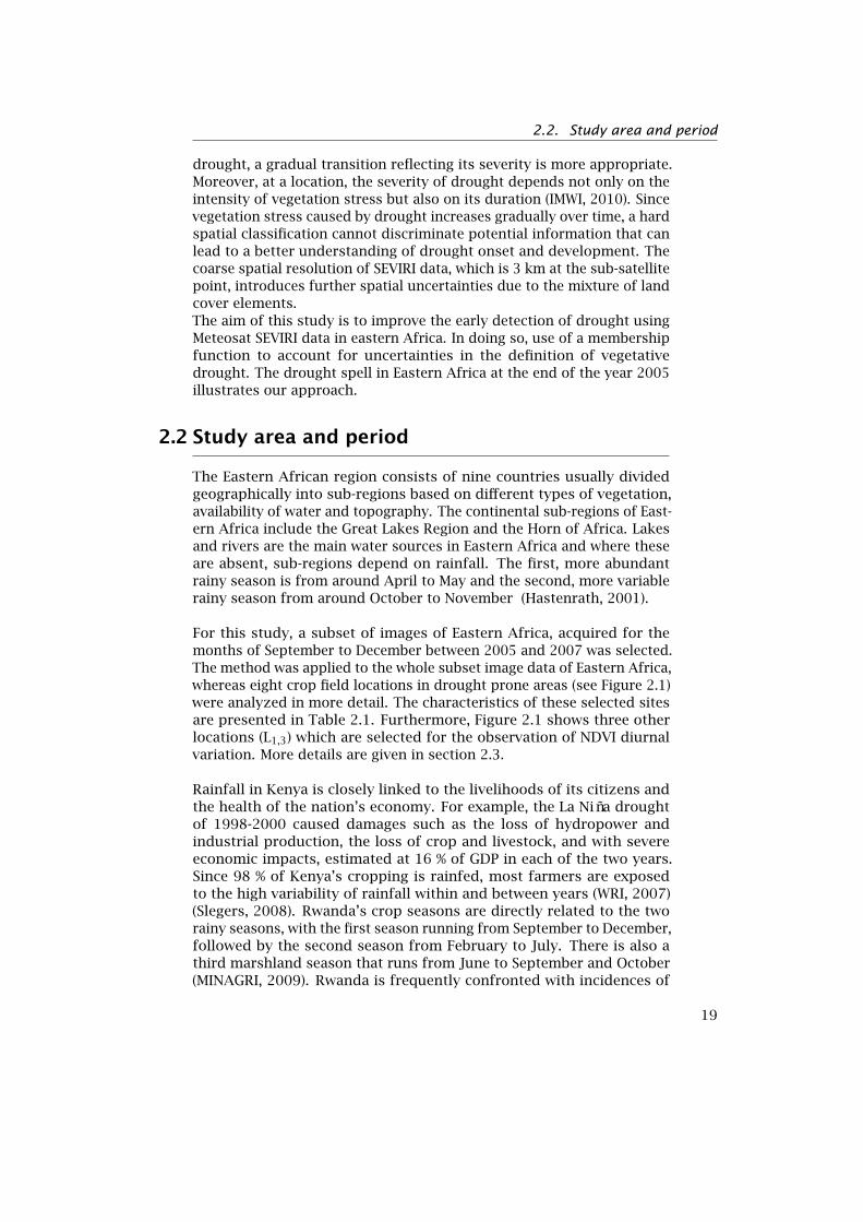
2.2 Study area and period
The Eastern African region consists of nine countries usually dividedgeographically into sub-regions based on different types of vegetation,availability of water and topography. The continental sub-regions of East-ern Africa include the Great Lakes Region and the Horn of Africa. Lakesand rivers are the main water sources in Eastern Africa and where theseare absent, sub-regions depend on rainfall. The first, more abundantrainy season is from around April to May and the second, more variablerainy season from around October to November (Hastenrath, 2001).
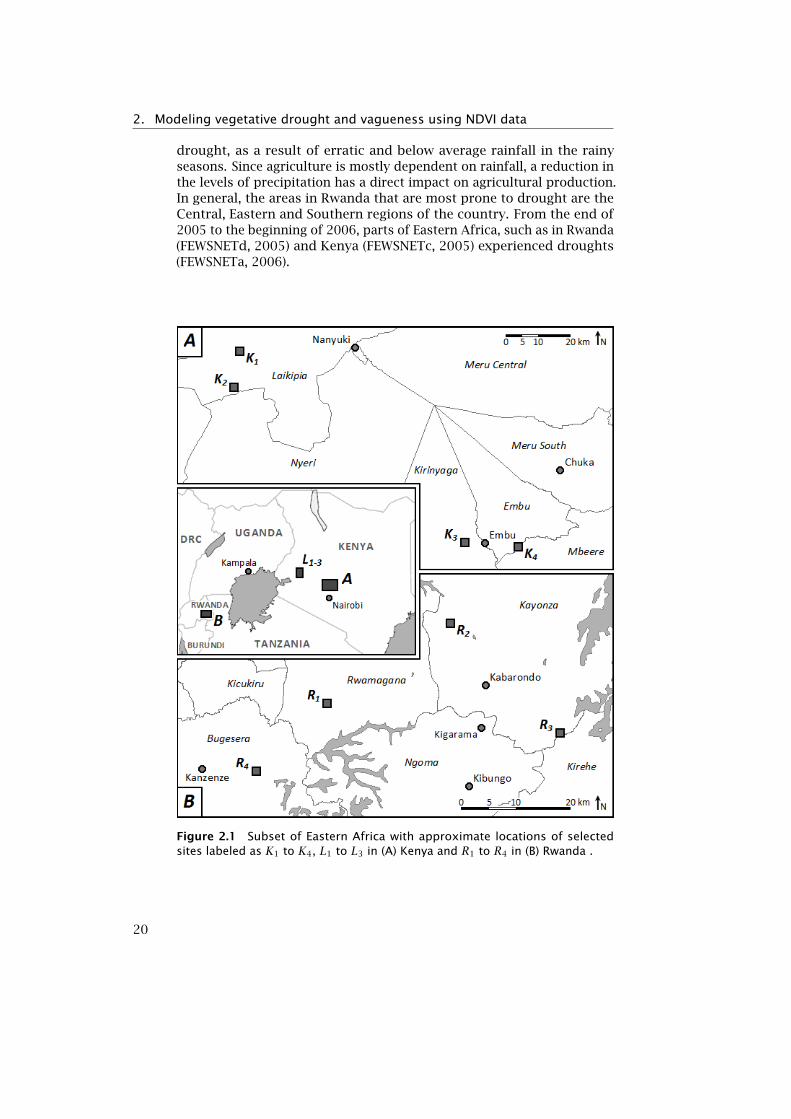
For this study, a subset of images of Eastern Africa, acquired for themonths of September to December between 2005 and 2007 was selected.The method was applied to the whole subset image data of Eastern Africa,whereas eight crop field locations in drought prone areas (see Figure 2.1)were analyzed in more detail. The characteristics of these selected sitesare presented in Table 2.1. Furthermore, Figure 2.1 shows three otherlocations (L1,3) which are selected for the observation of NDVI diurnalvariation. More details are given in section 2.3.
Rainfall in Kenya is closely linked to the livelihoods of its citizens andthe health of the nation’s economy. For example, the La Niña droughtof 1998-2000 caused damages such as the loss of hydropower andindustrial production, the loss of crop and livestock, and with severeeconomic impacts, estimated at 16 % of GDP in each of the two years.Since 98 % of Kenya’s cropping is rainfed, most farmers are exposedto the high variability of rainfall within and between years (WRI, 2007)(Slegers, 2008). Rwanda’s crop seasons are directly related to the tworainy seasons, with the first season running from September to December,followed by the second season from February to July. There is also athird marshland season that runs from June to September and October(MINAGRI, 2009). Rwanda is frequently confronted with incidences of
19
2. Modeling vegetative drought and vagueness using NDVI data
drought, as a result of erratic and below average rainfall in the rainyseasons. Since agriculture is mostly dependent on rainfall, a reduction inthe levels of precipitation has a direct impact on agricultural production.In general, the areas in Rwanda that are most prone to drought are theCentral, Eastern and Southern regions of the country. From the end of2005 to the beginning of 2006, parts of Eastern Africa, such as in Rwanda(FEWSNETd, 2005) and Kenya (FEWSNETc, 2005) experienced droughts(FEWSNETa, 2006).
Figure 2.1 Subset of Eastern Africa with approximate locations of selectedsites labeled as K1 to K4, L1 to L3 in (A) Kenya and R1 to R4 in (B) Rwanda .
20
2.3. Data acquisition and processing
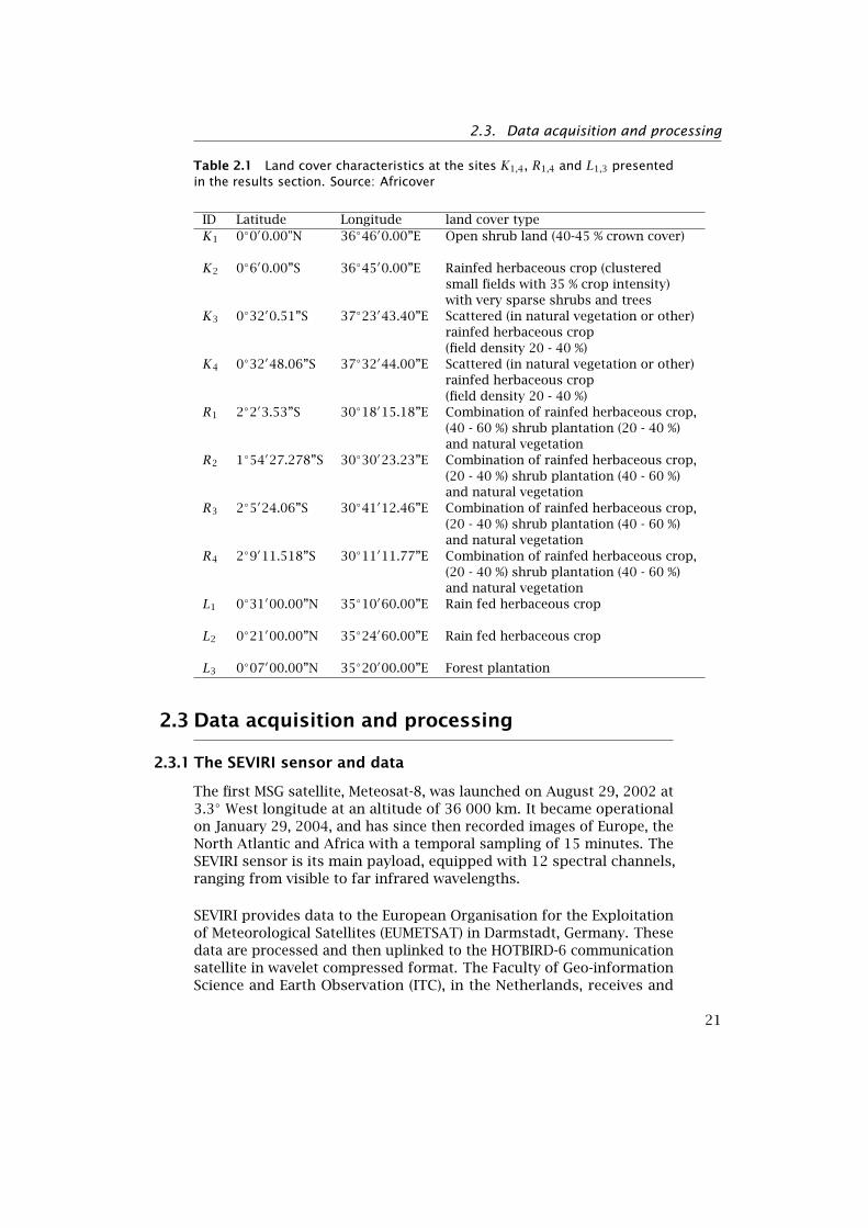
Table 2.1 Land cover characteristics at the sites K1,4, R1,4 and L1,3 presentedin the results section. Source: Africover
ID Latitude Longitude land cover typeK1 0◦0′0.00"N 36◦46′0.00”E Open shrub land (40-45 % crown cover)
K2 0◦6′0.00”S 36◦45′0.00”E Rainfed herbaceous crop (clusteredsmall fields with 35 % crop intensity)with very sparse shrubs and trees
K3 0◦32′0.51”S 37◦23′43.40”E Scattered (in natural vegetation or other)rainfed herbaceous crop(field density 20 - 40 %)
K4 0◦32′48.06”S 37◦32′44.00”E Scattered (in natural vegetation or other)rainfed herbaceous crop(field density 20 - 40 %)
R1 2◦2′3.53”S 30◦18′15.18”E Combination of rainfed herbaceous crop,(40 - 60 %) shrub plantation (20 - 40 %)and natural vegetation
R2 1◦54′27.278”S 30◦30′23.23”E Combination of rainfed herbaceous crop,(20 - 40 %) shrub plantation (40 - 60 %)and natural vegetation
R3 2◦5′24.06”S 30◦41′12.46”E Combination of rainfed herbaceous crop,(20 - 40 %) shrub plantation (40 - 60 %)and natural vegetation
R4 2◦9′11.518”S 30◦11′11.77”E Combination of rainfed herbaceous crop,(20 - 40 %) shrub plantation (40 - 60 %)and natural vegetation
L1 0◦31′00.00”N 35◦10′60.00”E Rain fed herbaceous crop
L2 0◦21′00.00”N 35◦24′60.00”E Rain fed herbaceous crop
L3 0◦07′00.00”N 35◦20′00.00”E Forest plantation
2.3 Data acquisition and processing
2.3.1 The SEVIRI sensor and data
The first MSG satellite, Meteosat-8, was launched on August 29, 2002 at3.3◦ West longitude at an altitude of 36 000 km. It became operationalon January 29, 2004, and has since then recorded images of Europe, theNorth Atlantic and Africa with a temporal sampling of 15 minutes. TheSEVIRI sensor is its main payload, equipped with 12 spectral channels,ranging from visible to far infrared wavelengths.
SEVIRI provides data to the European Organisation for the Exploitationof Meteorological Satellites (EUMETSAT) in Darmstadt, Germany. Thesedata are processed and then uplinked to the HOTBIRD-6 communicationsatellite in wavelet compressed format. The Faculty of Geo-informationScience and Earth Observation (ITC), in the Netherlands, receives and
21
2. Modeling vegetative drought and vagueness using NDVI data
archives these data in compressed form on drivers accessible throughpersonal computers on the network. Level 1.5 data were imported andconverted into Ilwis raster data format using the MSG Data Retriever(Maathuis et al., 2005) tool available at ITC, with the aid of a GeospatialData Abstraction Library (GDAL)-driver that reads raw compressed MSGdata and facilitates easy geometric and radiometric calibrated data re-trieval into formats commonly used by remote sensing packages.
In this study, bands one (VIS 0.6) (red, 0.56 − 0.71µm) and two (VIS0.8) (near infrared, 0.74− 0.88µm), converted into reflectance have beenused to calculate the NDVI. Images covering the region during the cropseason of September to December, for the years 2005, 2006 and 2007,were used. They were recorded between 06:00 UTC and 11:00 UTC,corresponding approximately to 08:00-09:00 to 13:00-14:00 local time,respectively.
The cloud mask product (CLM) distributed by EUMETSAT was appliedon each image. The DV values are calculated as in equation (2.1). Noatmospheric correction was carried out.
2.3.2 Precipitation data
In this study, precipitation data from August to November, 2005 to 2007,aggregated to 10 day period, were used to validate the results. These datawere taken from stations closest to the points selected for the droughtanalysis, i.e. respectively in Embu, Kenya and in Kigali, Rwanda. FromEmbu meteo station, K1 is located at approximately 93 km, K2 at 89 km,K3 at 7.5 km and K4 at 12 km. From Kigali meteo station, R1 is locatedapproximately at 21 km, R2 at 42 km, R3 at 63 km and R4 at 23 km. Datafor Embu were retrieved from the National Climatic Data Centre (NCDC,2010) and data for Kigali from the Rwandan Meteorological Service.Precipitation data for Embu are incomplete in 2005 for the 1st , 2nd and3rd dekad of August, and the 2nd dekad of November; in 2006 for the3rd dekad of August, the 2nd dekad of September, the 2nd dekad ofOctober and the 3rd dekad of November; and in 2007 for the 3rd dekadof October, and the 1st and 2nd dekad of November; as data for one ormore days within these 10-day periods is missing. The data for the 2nd
dekad of November have not been included in the chart of Figure 3.
2.3.3 Generation of the DV(t,s) time series
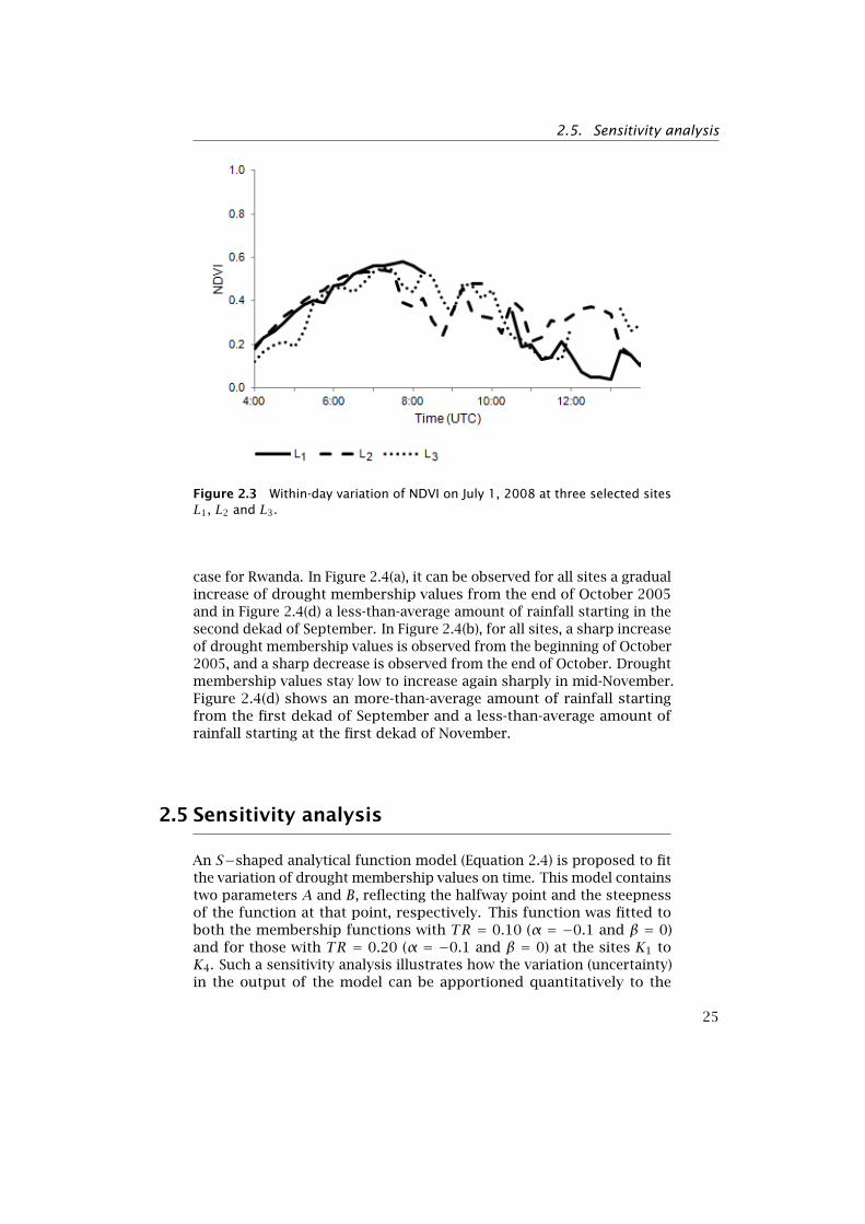
First, an observation of diurnal variation of NDVI was conducted on the01st of July 2008 at three locations (L1, L2 and L3) (Figure 2.1) in Kenyaduring a non-drought season. This particular day and these particularlocations were selected based on the fact that most cloud-free scenescould be obtained. The NDVI was calculated for every 15-minutes timeinterval. The observations, as shown in Figure 2.3, are assumed to bevalid for the eight study sites and as such, a time window between
22
2.3. Data acquisition and processing
06:00 and 11:00 UTC (09:00 and 14:00 local time) was selected to avoidincluding systematic low NDVI values. Second, the daily maximum NDVIcomposite was calculated for each of the selected sites. These dailyNDVI composites were further used to generate the four-days maximumNDVI composites. Daily NDVI time series were generated by determiningthe maximum NDVI value from the available 15 minute images duringa 5 hours observation window between 06:00 and 11:00 UTC, fromSeptember to December. This provided one daily value for these fourmonths over a period of three years. To reduce the number of missingvalues in this series, a period of four day maximum NDVI composites,consisting in total of 90 values was considered. Such a period of fourdays was selected as it was the minimum set with the least missing NDVIvalues. From the four - day maximum values, the mean values over 2005- 2007 for each period of 4 days (30 values from September to December)were calculated. To generate the DV(t,s) time series, these mean valueswere subtracted from the four-day composite time series. Finally, theseries was limited to the months of October and November in 2005, 2006and 2007 (number of images = 48 DV(t,s)).
2.3.4 Spatial modeling of vegetative drought
To model drought from vegetation condition, fuzzy sets theory wasused, thus accounting for the gradual transition between drought andnon-drought classes. Fuzzy sets theory, introduced by Zadeh (1965),provides a conceptual framework for solving knowledge representationand classification in an ambiguous environment. Elements of a fuzzyset can take values ranging from 0 to 1, unlike the traditionally used(boolean) set whose elements take either 0 or 1. This function allowsone to quantify the gradual evolution of vegetative drought at a loca-tion. Fuzzy sets theory has been used and discussed in remote sensingstudies of change detection analysis (Metternicht, 1999, 2001) and tomodel vague geographic entities (Fisher, 2000) (Woodcock and Gopal,2000) (Cheng et al., 2009).
The parameters of the transition range (TR), which should be definedbased on expert knowledge, were estimated arbitrarily in this study toillustrate the function. The shape of the function was selected on thebasis of the following assumptions:
• Vegetation stress observed on DV (t, s) images is caused by droughtcondition
• Variation of intensity of vegetation stress reflects linearly the vari-ation of drought severity
• Under natural conditions, the severity of vegetative drought evolvesgradually in time
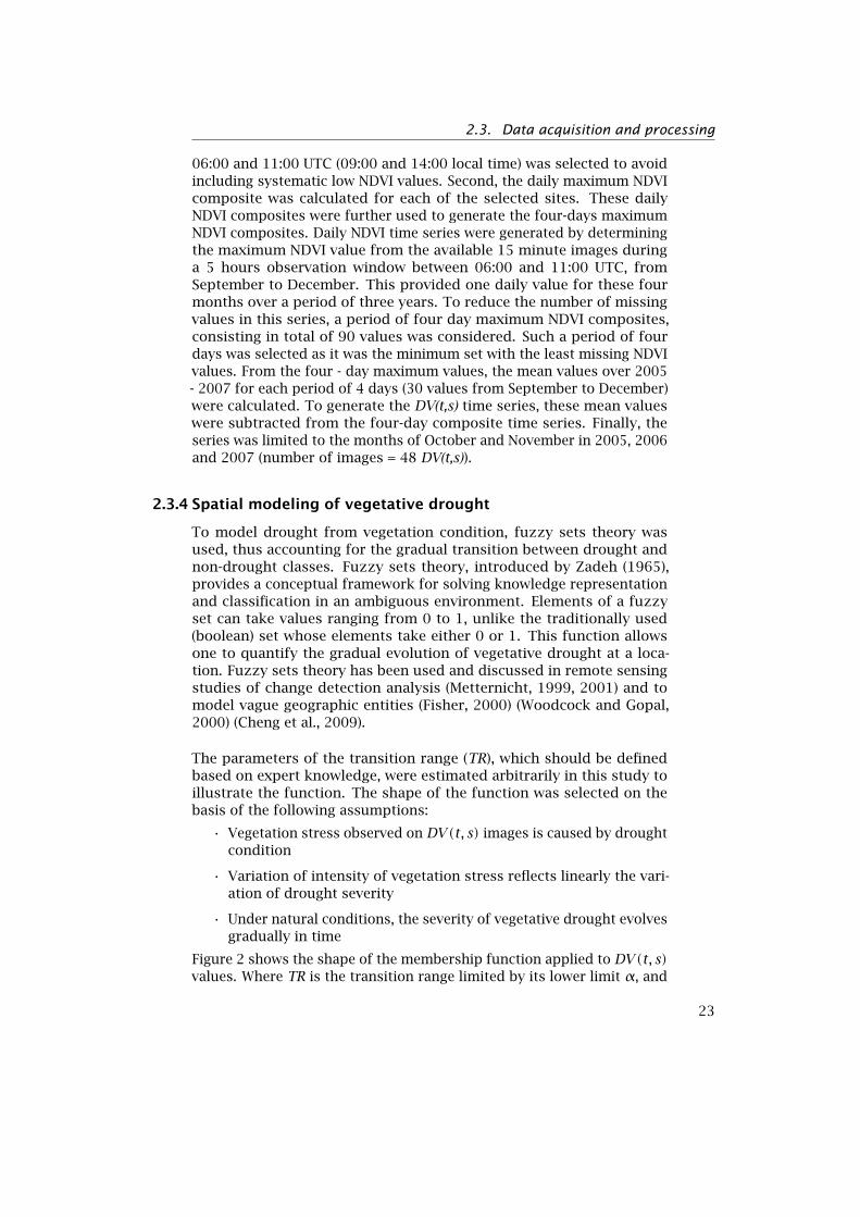
Figure 2 shows the shape of the membership function applied to DV (t, s)values. Where TR is the transition range limited by its lower limit α, and
23
2. Modeling vegetative drought and vagueness using NDVI data
Figure 2.2 Drought membership function d(x) applied to DV values.
its upper limit β. DVmin is the overall minimum DV calculated duringthe study period.
d(x)
1 ∀x : x ≤ αβ−xβ−α ∀x : α < x < β0 otherwise
(2.3)
The one-sided trapezoidal drought membership function, d(x) as definedin (2.3), takes the value 1 (or certain drought) for vegetation conditionvalues below α and the value 0 (or certain non-drought) for vegetationcondition values above β, with a gradual linear transition of droughtmembership values between 0 and 1, for vegetation condition valuesbetween α and β. The function was applied to the time series of DV (t, s).A few pixel locations in field crop areas of Kenya and Rwanda wereextracted and tracked over time. Results are presented and discussedrespectively in sections 2.4 and 2.6.
2.4 Experimental results
Figure 2.3 shows the 15-minutes interval diurnal variation of NDVI at L1,L2 and L3 on the 01st of July 2008. From the graph, an increase of NDVIvalues is observed in the morning between approximately 04:00 and07:00 UTC (07:00 and 10:00 local time), followed by a slow and gradualdecline towards the evening.
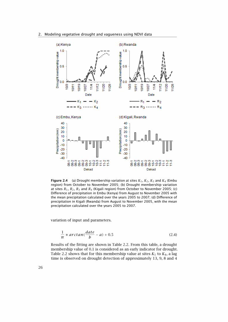
Figure 2.4(a) shows d(x) values calculated at sites K1 to K4 in Kenya,for the period from October to November 2005, in a four-day time scale,and Figure 4(b) shows d(x) values calculated at sites R1 to R4 in Rwanda,for the same period. The parameters α = −0.20 and β = 0 were setfor all sites. Figures 2.4(c) and 2.4(d) are the precipitation differencevalues for August to November 2005, from the mean 2005-2007. It canbe observed that for Embu, the increase in drought membership valuecoincides with less-than-average rainfall conditions, while this is not the
24
2.5. Sensitivity analysis
Figure 2.3 Within-day variation of NDVI on July 1, 2008 at three selected sitesL1, L2 and L3.
case for Rwanda. In Figure 2.4(a), it can be observed for all sites a gradualincrease of drought membership values from the end of October 2005and in Figure 2.4(d) a less-than-average amount of rainfall starting in thesecond dekad of September. In Figure 2.4(b), for all sites, a sharp increaseof drought membership values is observed from the beginning of October2005, and a sharp decrease is observed from the end of October. Droughtmembership values stay low to increase again sharply in mid-November.Figure 2.4(d) shows an more-than-average amount of rainfall startingfrom the first dekad of September and a less-than-average amount ofrainfall starting at the first dekad of November.
2.5 Sensitivity analysis
An S−shaped analytical function model (Equation 2.4) is proposed to fitthe variation of drought membership values on time. This model containstwo parameters A and B, reflecting the halfway point and the steepnessof the function at that point, respectively. This function was fitted toboth the membership functions with TR = 0.10 (α = −0.1 and β = 0)and for those with TR = 0.20 (α = −0.1 and β = 0) at the sites K1 toK4. Such a sensitivity analysis illustrates how the variation (uncertainty)in the output of the model can be apportioned quantitatively to the
25
2. Modeling vegetative drought and vagueness using NDVI data
Figure 2.4 (a) Drought membership variation at sites K1, K2, K3 and K4 (Emburegion) from October to November 2005; (b) Drought membership variationat sites R1, R2, R3 and R4 (Kigali region) from October to November 2005; (c)Difference of precipitation in Embu (Kenya) from August to November 2005 withthe mean precipitation calculated over the years 2005 to 2007; (d) Difference ofprecipitation in Kigali (Rwanda) from August to November 2005, with the meanprecipitation calculated over the years 2005 to 2007.
variation of input and parameters.
1π∗ arctan(date
b− a)+ 0.5 (2.4)
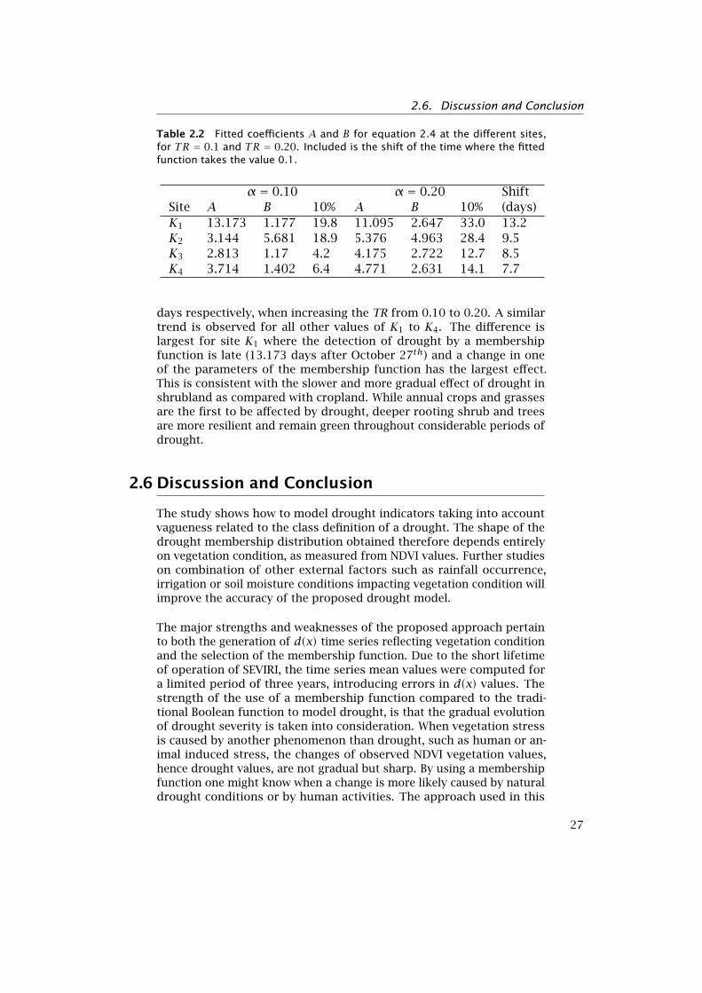
Results of the fitting are shown in Table 2.2. From this table, a droughtmembership value of 0.1 is considered as an early indicator for drought.Table 2.2 shows that for this membership value at sites K1 to K4, a lagtime is observed on drought detection of approximately 13, 9, 8 and 4
26
2.6. Discussion and Conclusion
Table 2.2 Fitted coefficients A and B for equation 2.4 at the different sites,for TR = 0.1 and TR = 0.20. Included is the shift of the time where the fittedfunction takes the value 0.1.
α = 0.10 α = 0.20 ShiftSite A B 10% A B 10% (days)K1 13.173 1.177 19.8 11.095 2.647 33.0 13.2K2 3.144 5.681 18.9 5.376 4.963 28.4 9.5K3 2.813 1.17 4.2 4.175 2.722 12.7 8.5K4 3.714 1.402 6.4 4.771 2.631 14.1 7.7
days respectively, when increasing the TR from 0.10 to 0.20. A similartrend is observed for all other values of K1 to K4. The difference islargest for site K1 where the detection of drought by a membershipfunction is late (13.173 days after October 27th) and a change in oneof the parameters of the membership function has the largest effect.This is consistent with the slower and more gradual effect of drought inshrubland as compared with cropland. While annual crops and grassesare the first to be affected by drought, deeper rooting shrub and treesare more resilient and remain green throughout considerable periods ofdrought.
2.6 Discussion and Conclusion
The study shows how to model drought indicators taking into accountvagueness related to the class definition of a drought. The shape of thedrought membership distribution obtained therefore depends entirelyon vegetation condition, as measured from NDVI values. Further studieson combination of other external factors such as rainfall occurrence,irrigation or soil moisture conditions impacting vegetation condition willimprove the accuracy of the proposed drought model.
The major strengths and weaknesses of the proposed approach pertainto both the generation of d(x) time series reflecting vegetation conditionand the selection of the membership function. Due to the short lifetimeof operation of SEVIRI, the time series mean values were computed fora limited period of three years, introducing errors in d(x) values. Thestrength of the use of a membership function compared to the tradi-tional Boolean function to model drought, is that the gradual evolutionof drought severity is taken into consideration. When vegetation stressis caused by another phenomenon than drought, such as human or an-imal induced stress, the changes of observed NDVI vegetation values,hence drought values, are not gradual but sharp. By using a membershipfunction one might know when a change is more likely caused by naturaldrought conditions or by human activities. The approach used in this
27
2. Modeling vegetative drought and vagueness using NDVI data
study to quantify drought can be used to optimize drought detectionand remove false alarm. To do so, one needs to select the shape ofthe function as well as parameters α and β, which require an a prioriknowledge of characteristics of vegetative drought at study sites. In thisstudy, the shape of the function of the drought membership functionand the parameters α and β have been chosen somewhat arbitrarilyto illustrate the approach. Further research is needed to optimize themodel.
A comparison with rainfall data was performed to assess the validity ofthe drought signal obtained, as NDVI is a response variable to rainfall.For Embu, the increase in drought membership value coincided withless-than-average rainfall conditions, as expected, especially for the twolocations (K3 and K4) closest to the Embu meteo station. However, forsites in Eastern Rwanda, this was not the case. I suppose this could becaused by the large distance between Kigali meteo station and the fourobservation sites, or by the relief difference between Kigali, which ishilly and near the central Plateau, and the South-Eastern part of Rwanda,which is flatter. As no rainfall data were available for areas closer to theobservation sites, this assumption could not be validated.
The high temporal resolution data from instruments such as SEVIRIoffers opportunities to address processes occurring in plants such asduration and intensity of photosynthetic activity and understanding ofplant phenology which previously could not be measured. The exploita-tion of these parameters can provide additional information which canbe beneficial in the context of drought monitoring; this is a potential areaof investigation for future studies. Fensholt et al. (2006) suggested thatthe NDVI bowl-shaped curve observed from the variation of Meteosat -derived NDVI in Senegal during the morning can infer canopy structure.Bijker (2007) found similar results while observing diurnal NDVI vari-ation in the Netherlands, however suggesting this pattern to be relatedto photosynthetic activity. From observations during a day with predom-inant clear sky (results not included in the paper), a similar bowl-shapedNDVI curve was observed on selected sites in Kenya. Future researchmay reveal whether taking such effects into account leads to substan-tial improvement in drought modeling. Fensholt et al. (2006) observedpeak values occurring around 10.45 local time and the study sites inKenya showed peak values of NDVI at around 11.00 am local time (Figure2.3). Future research in that area may also reveal whether taking such ef-fects into account leads to substantial improvement in drought modeling.
A next step in drought modeling could also be an approach focusing onspatial objects. To do so, objects have to be built from collected images.Drought objects will be necessarily vague and uncertain, likely showinglarge spatial within-object variation as well. The method proposed inthis study may serve as a first step into this direction. In fact, what isdone here for individual pixels can also be done for a group of pixels.
28

2.6. Discussion and Conclusion
In principle, these pixels could be combined by considering a series ofimages into a 3-dimensional space-time drought object. An α-cut equalto 0.1 or 0.5 may then delineate the final objects.
29

3Validating MSG-SEVIRI NDVIvalues in East Africa
3.1 Introduction 333.2 Dataset and study site 333.3 Methods 353.4 Results and discussion 383.5 Conclusion 43
This chapter is based on: C.M Rulinda, W. Bijker, A. Stein (2011). Thechlorophyll variability in meteosat derived NDVI in a context of droughtmonitoring. In: Procedia Environmental Sciences, 3, 1st conference onSpatial Statistics 2011 - Mapping Global Change, Enschede, 23-25 March2011.
31
3. Validating MSG-SEVIRI NDVI values in East Africa
Abstract
This study proposes a validation method for the Meteosat SEVIRI derivedNDVI values in regards to vegetation condition from ground observations.The percentage of vegetation cover and the chlorophyll content wereselected as vegetation condition variables and their variability within andbetween SEVIRI pixels were assessed. No significant variability was foundwithin pixels but between pixels for each of the variables. These variableswere compared first separately with NDVI values, and later combined,with the NDVI values composited at different time steps. Results showedthat the combination of variables had a similar trend than the meanNDVI and maximum NDVI values calculated for the whole period of thestudy, as the presence of clouds influenced the daily NDVI values. Thestudy concluded that NDVI values can be used without compromisingthe variability of chlorophyll content and percentage of vegetation coverwithin those pixels. This findings can be used to understand the variationof NDVI which can be observed during a drought period.
32
3.1. Introduction
3.1 Introduction
Remote Sensing images from the Spinning Enhanced Visible and InfraredImager (SEVIRI) sensor onboard the Meteosat Second Generation (MSG)satellites are increasingly being used to monitor vegetation dynamics, aswell as to quantify the impact of drought on vegetation (Fensholt et al.,2006) (Bijker, 2007),(Lacaze and Bergés, 2005). More recently, Rulindaet al. (2010) have used SEVIRI-NDVI images to specifically address veget-ative drought monitoring as a vague phenomenon.
These studies showed that due to their high temporal resolution, SEVIRIimages can offer the opportunity to reduce the effect of cloud contam-ination in NDVI by creating maximum composite values (MVC) over areduced period of time compared to other satellites images. In hetero-geneous vegetated areas, the coarse spatial resolution of these imageshowever can hinder their capacity to capture the spatial variability ofvegetation characteristics within a pixel, hence potentially underestimatevegetation, or particularly vegetative drought, dynamics in a region.
This study aims at validating the observed SEVIRI NDVI values. This isperformed by quantifying the spatial variability of vegetation condition,expressed in chlorophyll content and percentage vegetation cover, inSEVIRI pixels and compare it with NDVI values in order to understandtheir relationship. NDVI is a well known quantitative indicator of therelative abundance and activity of green vegetation and is well correlatedwith several biophysical characteristics of vegetation such as Leaf AreaIndex (LAI), percentage green cover, green biomass and chlorophyll con-tent (Jones and Vaughan, 2010).
In the next Section, the data set and study area are described, andin Section 3.3, the methods are presented. Section 3.4 presents anddiscusses the results of this study, and the last section concludes withrecommendations for future work.
3.2 Data set and Study site
3.2.1 Study area
The study was conducted over the heterogeneously vegetated area ofBugesera, which has also been recurrently affected by drought in the lastdecades. The district of Bugesera is located on the South Eastern plainsof Rwanda’s Eastern Province (Figure 3.1). It has a surface area of 1 337km2 (UNEP/UNDP/GOR, 2007) and is characterized by a large number oflakes, which approximate a total surface area of 106 km2.The altitude of Bugesera ranges between 1 300 m and 1 667 m and theregion is predominantly vegetated by dry savannas characterized byshort grasses, shrubs and short trees. The shrubs and short trees are
33
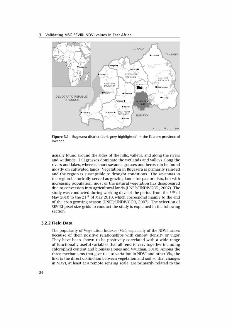
3. Validating MSG-SEVIRI NDVI values in East Africa
Figure 3.1 Bugesera district (dark grey highlighted) in the Eastern province ofRwanda.
usually found around the sides of the hills, valleys, and along the riversand wetlands. Tall grasses dominate the wetlands and valleys along therivers and lakes, whereas short savanna grasses and herbs can be foundmostly on cultivated lands. Vegetation in Bugesera is primarily rain-fedand the region is susceptible to drought conditions. The savannas inthe region historically served as grazing lands for pastoralists, but withincreasing population, most of the natural vegetation has disappeareddue to conversion into agricultural lands (UNEP/UNDP/GOR, 2007). Thestudy was conducted during working days of the period from the 5th ofMay 2010 to the 21st of May 2010, which correspond mainly to the endof the crop growing season (UNEP/UNDP/GOR, 2007). The selection ofSEVIRI-pixel size grids to conduct the study is explained in the followingsection.
3.2.2 Field Data
The popularity of Vegetation Indexes (VIs), especially of the NDVI, arisesbecause of their positive relationships with canopy density or vigor.They have been shown to be positively correlated with a wide rangeof functionally useful variables that all tend to vary together includingchlorophyll content and biomass (Jones and Vaughan, 2010). Among thethree mechanisms that give rise to variation in NDVI and other VIs, thefirst is the direct distinction between vegetation and soil so that changesin NDVI, at least at a remote sensing scale, are primarily related to the
34
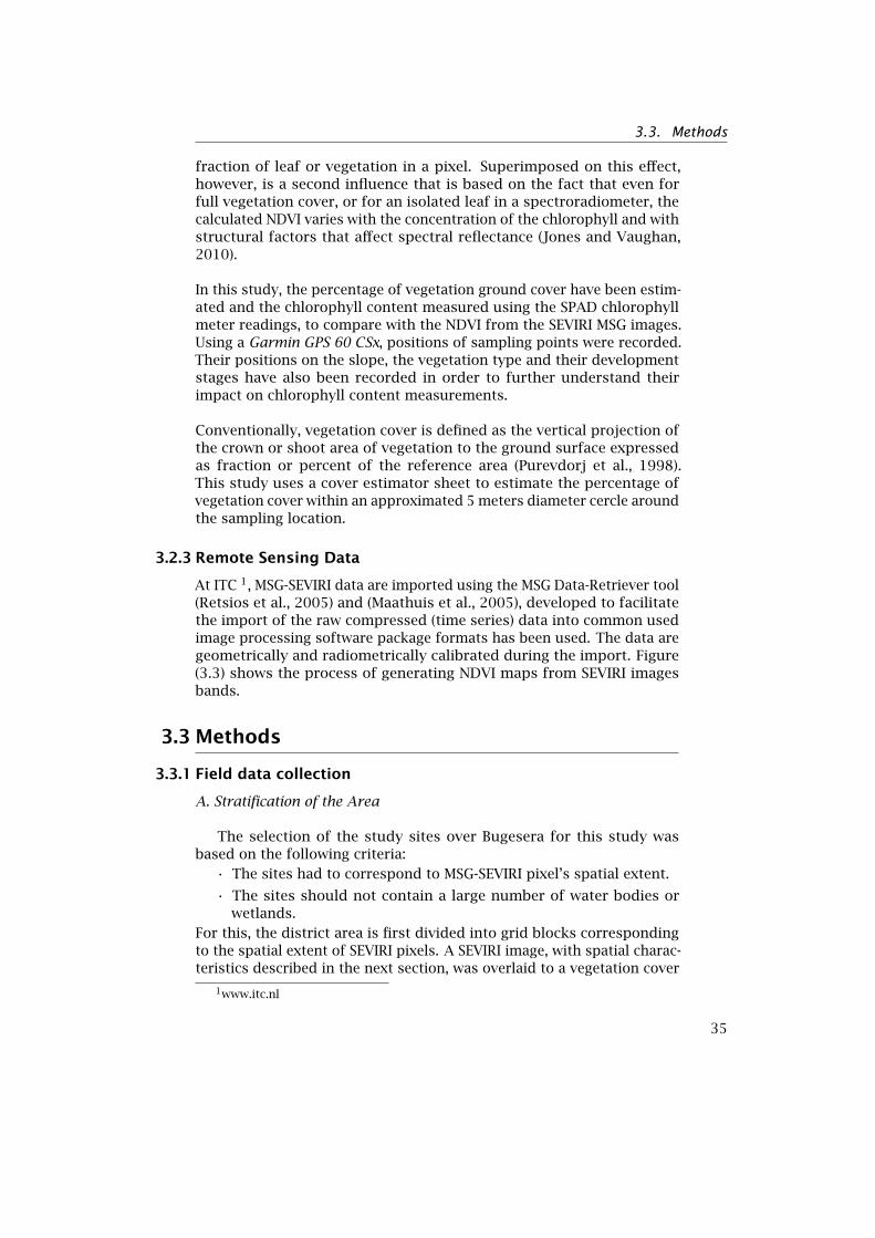
3.3. Methods
fraction of leaf or vegetation in a pixel. Superimposed on this effect,however, is a second influence that is based on the fact that even forfull vegetation cover, or for an isolated leaf in a spectroradiometer, thecalculated NDVI varies with the concentration of the chlorophyll and withstructural factors that affect spectral reflectance (Jones and Vaughan,2010).
In this study, the percentage of vegetation ground cover have been estim-ated and the chlorophyll content measured using the SPAD chlorophyllmeter readings, to compare with the NDVI from the SEVIRI MSG images.Using a Garmin GPS 60 CSx, positions of sampling points were recorded.Their positions on the slope, the vegetation type and their developmentstages have also been recorded in order to further understand theirimpact on chlorophyll content measurements.
Conventionally, vegetation cover is defined as the vertical projection ofthe crown or shoot area of vegetation to the ground surface expressedas fraction or percent of the reference area (Purevdorj et al., 1998).This study uses a cover estimator sheet to estimate the percentage ofvegetation cover within an approximated 5 meters diameter cercle aroundthe sampling location.
3.2.3 Remote Sensing Data
At ITC 1, MSG-SEVIRI data are imported using the MSG Data-Retriever tool(Retsios et al., 2005) and (Maathuis et al., 2005), developed to facilitatethe import of the raw compressed (time series) data into common usedimage processing software package formats has been used. The data aregeometrically and radiometrically calibrated during the import. Figure(3.3) shows the process of generating NDVI maps from SEVIRI imagesbands.
3.3 Methods
3.3.1 Field data collection
A. Stratification of the Area
The selection of the study sites over Bugesera for this study wasbased on the following criteria:
• The sites had to correspond to MSG-SEVIRI pixel’s spatial extent.
• The sites should not contain a large number of water bodies orwetlands.
For this, the district area is first divided into grid blocks correspondingto the spatial extent of SEVIRI pixels. A SEVIRI image, with spatial charac-teristics described in the next section, was overlaid to a vegetation cover
1www.itc.nl
35
3. Validating MSG-SEVIRI NDVI values in East Africa
Figure 3.2 Grid blocks pre-selected based on land cover classification andmatching with SEVIRI images pixel extent. The five grids are displayed overthe land cover map generalized from the AFRICOVER 2000 land cover map ofRwanda.
map of Bugesera, generalized from the Africover land cover map. Gridscontaining the less amount of water bodies and Wetlands are then pre-selected. The region of Bugesera containing a large area of water bodies,only 5 grids are pre-selected (Figure 3.2). Among these five pre-selectedgrids, only four could be sampled as the fifth one was found to be on amilitary property at the time of the field work.
B. Random sampling
A hundred random points were generated for the whole district ofBugesera, using ArcGIS. Two transects were set up deliberately in East-West and North-South directions, each intersecting at one random pointat least, in every grid. These two East-West and North-South transectsper grid are laid in order to account for potential directional influence of
36
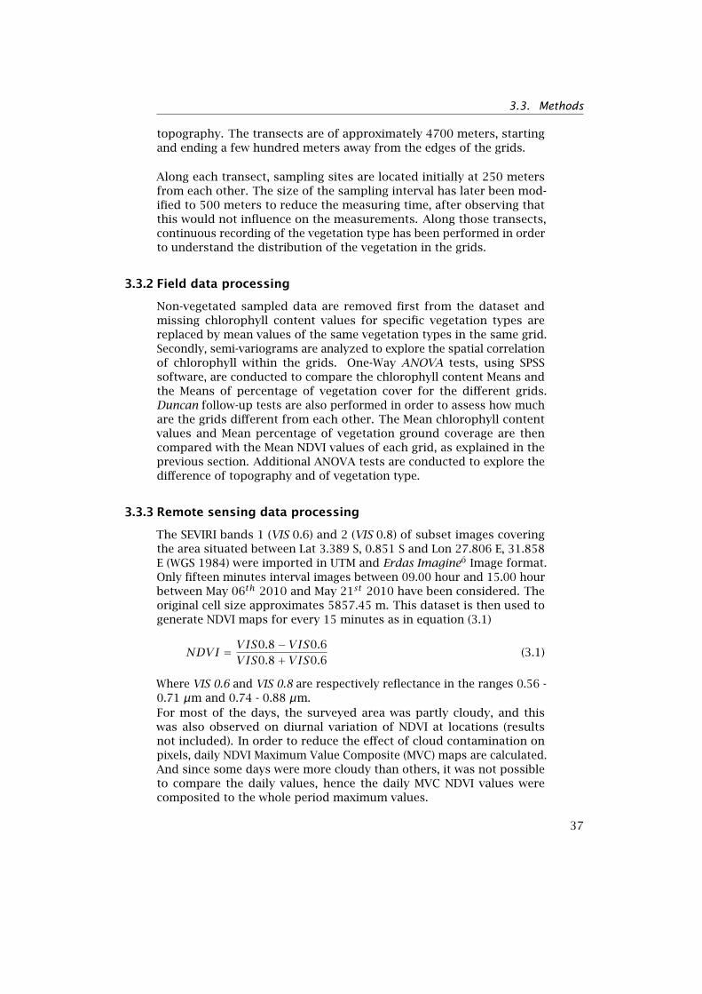
3.3. Methods
topography. The transects are of approximately 4700 meters, startingand ending a few hundred meters away from the edges of the grids.
Along each transect, sampling sites are located initially at 250 metersfrom each other. The size of the sampling interval has later been mod-ified to 500 meters to reduce the measuring time, after observing thatthis would not influence on the measurements. Along those transects,continuous recording of the vegetation type has been performed in orderto understand the distribution of the vegetation in the grids.
3.3.2 Field data processing
Non-vegetated sampled data are removed first from the dataset andmissing chlorophyll content values for specific vegetation types arereplaced by mean values of the same vegetation types in the same grid.Secondly, semi-variograms are analyzed to explore the spatial correlationof chlorophyll within the grids. One-Way ANOVA tests, using SPSSsoftware, are conducted to compare the chlorophyll content Means andthe Means of percentage of vegetation cover for the different grids.Duncan follow-up tests are also performed in order to assess how muchare the grids different from each other. The Mean chlorophyll contentvalues and Mean percentage of vegetation ground coverage are thencompared with the Mean NDVI values of each grid, as explained in theprevious section. Additional ANOVA tests are conducted to explore thedifference of topography and of vegetation type.
3.3.3 Remote sensing data processing
The SEVIRI bands 1 (VIS 0.6) and 2 (VIS 0.8) of subset images coveringthe area situated between Lat 3.389 S, 0.851 S and Lon 27.806 E, 31.858E (WGS 1984) were imported in UTM and Erdas Imagineo Image format.Only fifteen minutes interval images between 09.00 hour and 15.00 hourbetween May 06th 2010 and May 21st 2010 have been considered. Theoriginal cell size approximates 5857.45 m. This dataset is then used togenerate NDVI maps for every 15 minutes as in equation (3.1)
NDVI = VIS0.8− VIS0.6VIS0.8+ VIS0.6
(3.1)
Where VIS 0.6 and VIS 0.8 are respectively reflectance in the ranges 0.56 -0.71 µm and 0.74 - 0.88 µm.For most of the days, the surveyed area was partly cloudy, and thiswas also observed on diurnal variation of NDVI at locations (resultsnot included). In order to reduce the effect of cloud contamination onpixels, daily NDVI Maximum Value Composite (MVC) maps are calculated.And since some days were more cloudy than others, it was not possibleto compare the daily values, hence the daily MVC NDVI values werecomposited to the whole period maximum values.
37
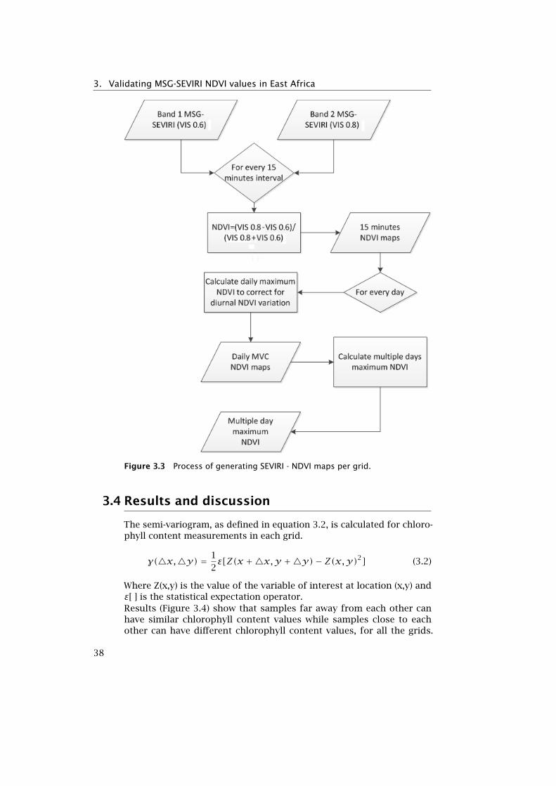
3. Validating MSG-SEVIRI NDVI values in East Africa
Figure 3.3 Process of generating SEVIRI - NDVI maps per grid.
3.4 Results and discussion
The semi-variogram, as defined in equation 3.2, is calculated for chloro-phyll content measurements in each grid.
γ(4x,4y) = 12ε[Z(x +4x,y +4y)− Z(x,y)2] (3.2)
Where Z(x,y) is the value of the variable of interest at location (x,y) andε[ ] is the statistical expectation operator.Results (Figure 3.4) show that samples far away from each other canhave similar chlorophyll content values while samples close to eachother can have different chlorophyll content values, for all the grids.
38
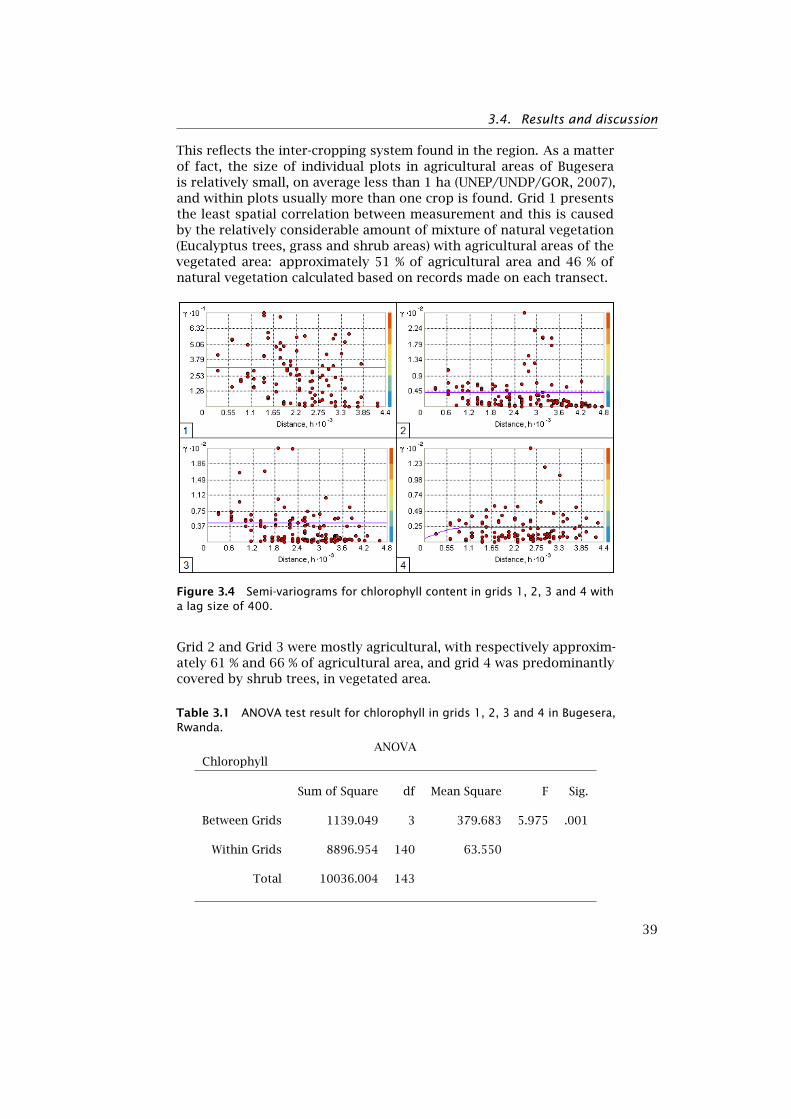
3.4. Results and discussion
This reflects the inter-cropping system found in the region. As a matterof fact, the size of individual plots in agricultural areas of Bugeserais relatively small, on average less than 1 ha (UNEP/UNDP/GOR, 2007),and within plots usually more than one crop is found. Grid 1 presentsthe least spatial correlation between measurement and this is causedby the relatively considerable amount of mixture of natural vegetation(Eucalyptus trees, grass and shrub areas) with agricultural areas of thevegetated area: approximately 51 % of agricultural area and 46 % ofnatural vegetation calculated based on records made on each transect.
Figure 3.4 Semi-variograms for chlorophyll content in grids 1, 2, 3 and 4 witha lag size of 400.
Grid 2 and Grid 3 were mostly agricultural, with respectively approxim-ately 61 % and 66 % of agricultural area, and grid 4 was predominantlycovered by shrub trees, in vegetated area.
Table 3.1 ANOVA test result for chlorophyll in grids 1, 2, 3 and 4 in Bugesera,Rwanda.
ANOVAChlorophyll
Sum of Square df Mean Square F Sig.
Between Grids 1139.049 3 379.683 5.975 .001
Within Grids 8896.954 140 63.550
Total 10036.004 143
39
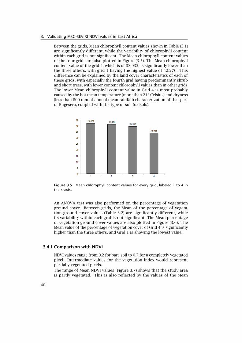
3. Validating MSG-SEVIRI NDVI values in East Africa
Between the grids, Mean chlorophyll content values shown in Table (3.1)are significantly different, while the variability of chlorophyll contentwithin each grid is not significant. The Mean chlorophyll content valuesof the four grids are also plotted in Figure (3.5). The Mean chlorophyllcontent value of the grid 4, which is of 33.935, is significantly lower thanthe three others, with grid 1 having the highest value of 42.276. Thisdifference can be explained by the land cover characteristics of each ofthese grids, with especially the fourth grid having predominantly shruband short trees, with lower content chlorophyll values than in other grids.The lower Mean chlorophyll content value in Grid 4 is most probablycaused by the hot mean temperature (more than 21◦ Celsius) and dryness(less than 800 mm of annual mean rainfall) characterization of that partof Bugesera, coupled with the type of soil (oxisols).
Figure 3.5 Mean chlorophyll content values for every grid, labeled 1 to 4 inthe x-axis.
An ANOVA test was also performed on the percentage of vegetationground cover. Between grids, the Mean of the percentage of vegeta-tion ground cover values (Table 3.2) are significantly different, whileits variability within each grid is not significant. The Mean percentageof vegetation ground cover values are also plotted in Figure (3.6). TheMean value of the percentage of vegetation cover of Grid 4 is significantlyhigher than the three others, and Grid 1 is showing the lowest value.
3.4.1 Comparison with NDVI
NDVI values range from 0.2 for bare soil to 0.7 for a completely vegetatedpixel. Intermediate values for the vegetation index would representpartially vegetated pixels.
The range of Mean NDVI values (Figure 3.7) shows that the study areais partly vegetated. This is also reflected by the values of the Mean
40
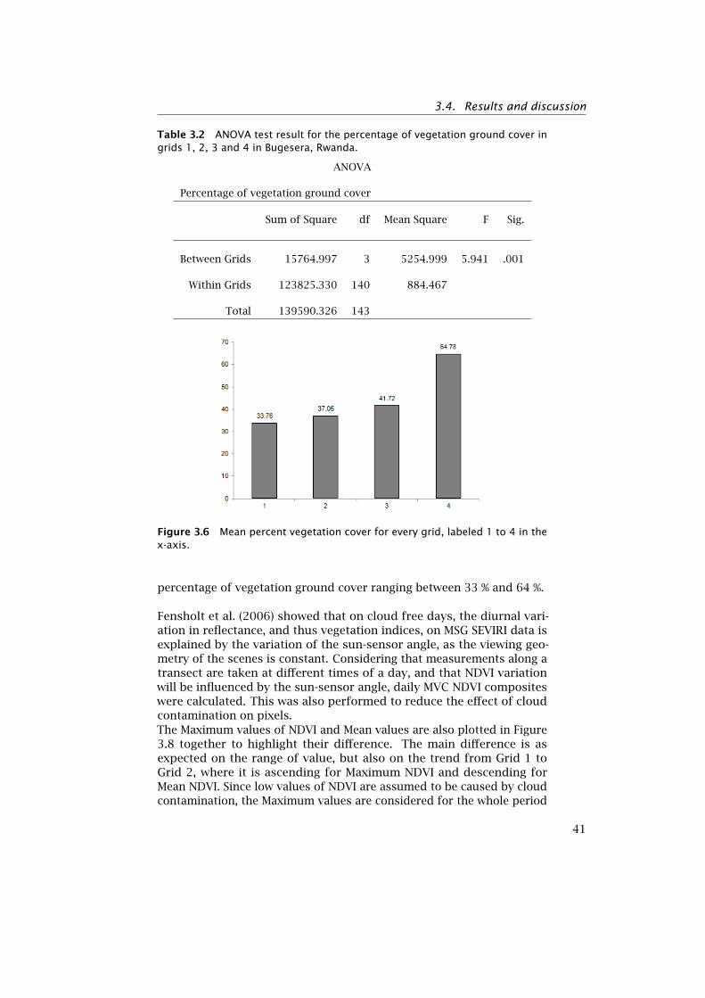
3.4. Results and discussion
Table 3.2 ANOVA test result for the percentage of vegetation ground cover ingrids 1, 2, 3 and 4 in Bugesera, Rwanda.
ANOVA
Percentage of vegetation ground cover
Sum of Square df Mean Square F Sig.
Between Grids 15764.997 3 5254.999 5.941 .001
Within Grids 123825.330 140 884.467
Total 139590.326 143
Figure 3.6 Mean percent vegetation cover for every grid, labeled 1 to 4 in thex-axis.
percentage of vegetation ground cover ranging between 33 % and 64 %.
Fensholt et al. (2006) showed that on cloud free days, the diurnal vari-ation in reflectance, and thus vegetation indices, on MSG SEVIRI data isexplained by the variation of the sun-sensor angle, as the viewing geo-metry of the scenes is constant. Considering that measurements along atransect are taken at different times of a day, and that NDVI variationwill be influenced by the sun-sensor angle, daily MVC NDVI compositeswere calculated. This was also performed to reduce the effect of cloudcontamination on pixels.The Maximum values of NDVI and Mean values are also plotted in Figure3.8 together to highlight their difference. The main difference is asexpected on the range of value, but also on the trend from Grid 1 toGrid 2, where it is ascending for Maximum NDVI and descending forMean NDVI. Since low values of NDVI are assumed to be caused by cloudcontamination, the Maximum values are considered for the whole period
41
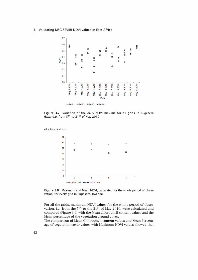
3. Validating MSG-SEVIRI NDVI values in East Africa
Figure 3.7 Variation of the daily NDVI maxima for all grids in Bugesera(Rwanda), from 5th to 21st of May 2010
of observation.
Figure 3.8 Maximum and Mean NDVI, calculated for the whole period of obser-vation, for every grid in Bugesera, Rwanda.
For all the grids, maximum NDVI values for the whole period of obser-vation, i.e. from the 5th to the 21st of May 2010, were calculated andcompared (Figure 3.9) with the Mean chlorophyll content values and theMean percentage of the vegetation ground cover.The comparison of Mean Chlorophyll content values and Mean Percent-age of vegetation cover values with Maximum NDVI values showed that
42
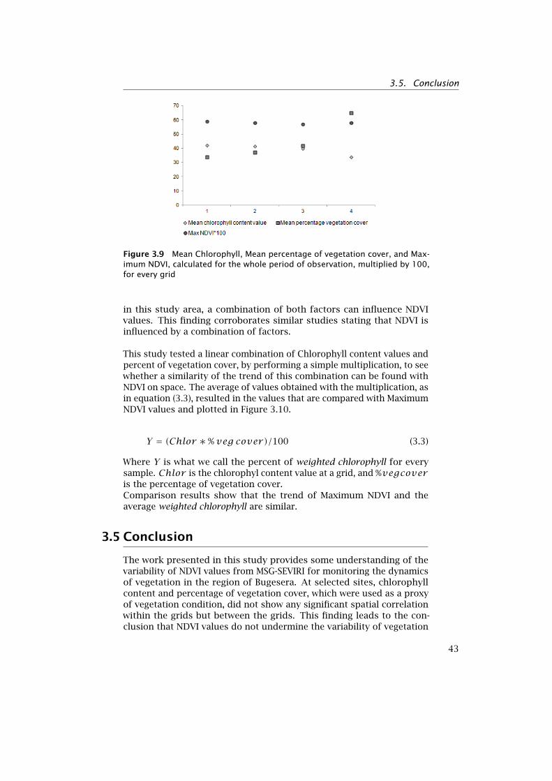
3.5. Conclusion
Figure 3.9 Mean Chlorophyll, Mean percentage of vegetation cover, and Max-imum NDVI, calculated for the whole period of observation, multiplied by 100,for every grid
in this study area, a combination of both factors can influence NDVIvalues. This finding corroborates similar studies stating that NDVI isinfluenced by a combination of factors.
This study tested a linear combination of Chlorophyll content values andpercent of vegetation cover, by performing a simple multiplication, to seewhether a similarity of the trend of this combination can be found withNDVI on space. The average of values obtained with the multiplication, asin equation (3.3), resulted in the values that are compared with MaximumNDVI values and plotted in Figure 3.10.
Y = (Chlor ∗ % veg cover)/100 (3.3)
Where Y is what we call the percent of weighted chlorophyll for everysample. Chlor is the chlorophyl content value at a grid, and %vegcoveris the percentage of vegetation cover.Comparison results show that the trend of Maximum NDVI and theaverage weighted chlorophyll are similar.
3.5 Conclusion
The work presented in this study provides some understanding of thevariability of NDVI values from MSG-SEVIRI for monitoring the dynamicsof vegetation in the region of Bugesera. At selected sites, chlorophyllcontent and percentage of vegetation cover, which were used as a proxyof vegetation condition, did not show any significant spatial correlationwithin the grids but between the grids. This finding leads to the con-clusion that NDVI values do not undermine the variability of vegetation
43
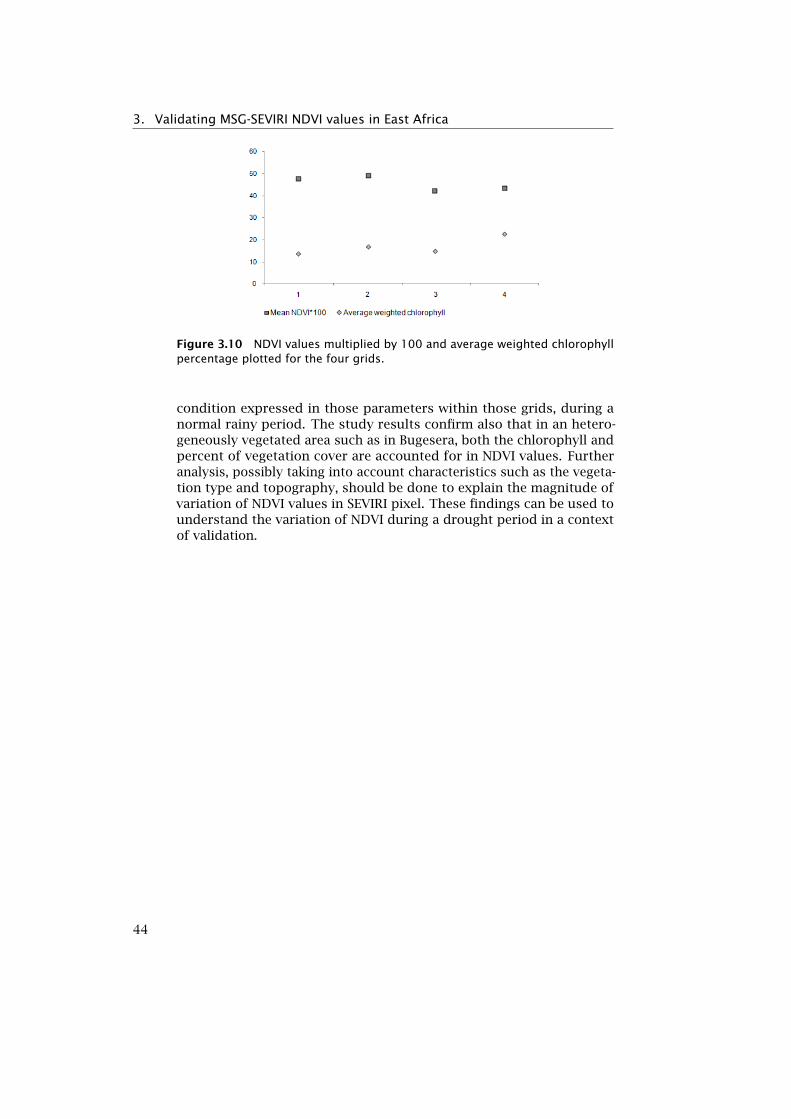
3. Validating MSG-SEVIRI NDVI values in East Africa
Figure 3.10 NDVI values multiplied by 100 and average weighted chlorophyllpercentage plotted for the four grids.
condition expressed in those parameters within those grids, during anormal rainy period. The study results confirm also that in an hetero-geneously vegetated area such as in Bugesera, both the chlorophyll andpercent of vegetation cover are accounted for in NDVI values. Furtheranalysis, possibly taking into account characteristics such as the vegeta-tion type and topography, should be done to explain the magnitude ofvariation of NDVI values in SEVIRI pixel. These findings can be used tounderstand the variation of NDVI during a drought period in a contextof validation.
44
4Quantifying spatial extent andvagueness of vegetative drought
4.1 Introduction 474.2 Previous work 484.3 Study area and data 494.4 Methodology 504.5 Results and discussion 554.6 Conclusion 60
This chapter is based on: C.M. Rulinda, A. Dilo, W. Bijker, A. Stein (2012).Characterizing and quantifying vegetative drought in East Africa usingfuzzy modelling and NDVI data. Journal of Arid Environments, 78, 169-178.
45
4. Quantifying spatial extent and vagueness of vegetative drought
Abstract
This study aims at improving the quantification of vegetative droughtas a vague spatial phenomenon. 10-day NOAA-AVHRR NDVI images ofEast Africa from September 2005 to April 2006 were used. Vegetativedrought was characterised using a membership function to model thegradual transition between drought and non-drought classes. Measureswere implemented to quantify the spatial extent (area) and vaguenessof vegetative drought, and to visualize its evolution in space and time.Results show a severe drought, affecting more than 60 % of the vegetatedarea in the region. Different degrees of vagueness were observed intime, independently of the width of the transition range; the vaguenessremained higher at the onset than at the termination of drought, re-flecting a more gradual onset of drought and a crisper return to normalconditions. The vagueness was the lowest at the drought peak. Themean-area was less vulnerable to the change of the transition range,compared to the core-area. A crisp approach, using the median of thetransition range as the threshold did not quantify its vagueness. Thismethod can also be used in other regions, or adapted to characterize andquantify other vague spatial phenomena.
46
4.1. Introduction
4.1 Introduction
In East Africa, the dynamics of vegetation strongly depend on wateravailability (Unganai and Kogan, 1998),(Sannier et al., 1998),(Nicholsonet al., 1990). Drought episodes reported in the past years have periodic-ally negatively affected the vegetation health in the region. For instance,during the end of the year 2005 and the beginning of the year 2006,the US Famine Early Warning System Network (FEWS NET), the Food andAgriculture Organization (FAO), and local institutions have all reported asevere drought episode that resulted in crop failure, pasture degradation,and water shortage, leading to a severe food insecurity in most parts ofEast Africa 1. In subsequent years, drought episodes were also reportedmostly in parts of Kenya, Somalia and Ethiopia, resulting in food crises.It is in this context that timely and affordable ways to assess the impactof drought on vegetation, especially in regions with limited ground collec-ted data, has been identified as an important factor to improve strategiesof drought mitigation (Ambenje, 2000) and reduce the negative impact.
Droughts are complex to quantify due to their creeping nature; theyaccumulate slowly and extend over long periods of time (Wilhite, 2005).The areas affected by drought evolve gradually as the symptoms of mois-ture stress in plants often develop slowly. In the process of modelingthe impact of drought on vegetation, hereafter referred to as vegetativedrought or drought, it is standard practice to use a crisp classification onvegetation stress values. This approach does not reflect the vague natureof drought, and hence could hinder its detection. Frank (2008) suggestedthat a realistic model could be a more critical issue in improving decisionmaking processes than the quality of input data. In this context wefocus on reflecting the vague nature of vegetative drought using a morerealistic model, hence improve its detection.
This study aims at improving the quantification of vegetative drought bytaking into account its vagueness. Measures are presented to quantifyvegetative drought at a regional scale and using remote sensing data asinput. The proposed measures to quantify vegetative drought are thetotal-area, the core-area, the mean-area and the vagueness, whichare explained in Section 4.4. The study also tracks drought objects in theimages and calculate their centroids, which are used to visualise theirevolution in space and time.
The rest of the chapter is organised in the following way: Section 4.2briefly presents previous work on vegetative drought monitoring; Section4.3 presents the characteristics of the study area and the data; Section4.4 details the methods; Section 4.5 presents and discusses the results,and is followed by a conclusion in Section 4.6.
1www.fews.net: the USAID FEWS NET Weather Hazards Impacts Assessment for Africa
47
4. Quantifying spatial extent and vagueness of vegetative drought
4.2 Previous work
Remote sensing data proved to be of a significant value in monitoringvegetation (Diouf and Lambini, 2001),(Sannier et al., 1998) and more spe-cifically drought (Tucker and Choudhury, 1987), (Liu and Kogan, 1996),(Ambenje, 2000), (Quan and Tenhunen, 2004), (Song et al., 2004),(Gouviaet al., 2009), (Lacaze and Bergés, 2005), (Peters et al., 2002) using multi-temporal data (Kogan, 2001). Although vegetative drought is difficult toidentify, it can be measured using various indicators that provide meansof monitoring (Dracup et al., 1980). In this context, the NormalizedDifference Vegetation Index (NDVI) (Tucker, 1979) is often used (Tuckerand Choudhury, 1987), (Ji and Peters, 2003).
Among the NDVI-based approach studies, Song et al. (2004) produced10-day (dekad) classified drought risk maps using the difference betweenthe current NDVI and the corresponding 3-year average from the Na-tional Oceanic and Atmospheric Administration-Advanced Very HighResolution Radiometer (NOAA-AVHRR). Pixels with difference NDVI val-ues below -0.1 were considered as drought risk areas, while pixels withdifference NDVI values below -0.25 were considered as severe droughtareas. On a monthly basis and using the Satéllite Pour l’Observation dela Terre (SPOT)-Vegetation NDVI data, Gouvia et al. (2009) estimated thearea of stressed vegetation in Portugal based on the number of pixelswith difference NDVI lower than -0.025. These NDVI anomalies werecomputed as the departure from the median of that month calculatedfor 8 years. Generally speaking, the NDVI-based approaches (Sannieret al., 1998), (Leelaruban et al., 2010), (Gouvia et al., 2009), althoughcharacterising and quantifying vegetative drought, are limited in the waythat they use the crisp classification method, hence do not account forthe vague nature of vegetative drought.
Significant progress has been made, using the fuzzy set theory (Zadeh,1965), to describe, store, process, and display vague objects (Dilo et al.,2007b,a), (Cheng et al., 2009), (Schneider, 1999), (Pauly and Schneider,2010), (Kanjilal et al., 2010). Methods were also developed in this per-spective to characterise vague spatial entities such as soil types (Bur-rough, 1989), forests types (Brown, 1998), and land use (Cheng et al.,2001). This study uses a fuzzy approach to model the gradual transitionbetween non-drought and drought. It uses measures developed for vagueobjects (Dilo et al., 2007b,a) modified for raster images. To visualise theevolution of drought in space and time, Dynomap, a software developedby Turdukulov et al. (2005) to track and visualise the evolution of imagefeatures in time-series, is used.
48
4.3. Study area and Data
4.3 Study area and Data
4.3.1 East Africa
This study is conducted over the area of East Africa (Figure 1.6). EastAfrica is situated approximately between 5◦30’N, 12◦S and 28◦05’E,41◦50’E and comprises mainly Burundi, Kenya, Rwanda, Tanzania, andUganda. The images include also the northern part of Zambia, portionsof South Sudan and South Somalia.
East Africa is predominantly semi-arid with an average rainfall amountof less than 800 mm per year; and sub-humid with an average rainfallamount varying between 800 and 1,300 mm per year (Vlek et al., 2008).Most parts of the region experience two rainy seasons per year: the firstone runs from around April to July and the second one, more variable,runs from around October to December.
The vegetation of East Africa is predominantly rain-fed and agriculturehas a key impact on the economy of the region, with approximately 80%of the combined population of Burundi, Kenya, Rwanda, Tanzania, andUganda depending on agriculture for their livelihood.
4.3.2 Drought in East Africa
In January 2006, the US National Aeronautics and Space Administration(NASA) Earth Observatory 2 reported that the failure of the short-seasonrains left large sections of East Africa in severe drought at the end ofthe year 2005 and early 2006. In a normal year, most of these affectedregions experience rainfall from March to May during the long rainyseason, and from October to December during the short rainy season.In 2005, the long rainy season produced little rain while the short rainyseason failed. The FEWSNET reported that as a result, the rainfall totalsfor the year were only 20-60 percent of normal, depending on the region.
The FEWSNET also reported that the impact of drought has been severe,resulting in crop failures, pasture degradation, water shortages, andhas raised serious food security concerns for the region. By the end ofJanuary 2006, millions were in need of food aid, particularly pastoralistswho depend on rain-fed pasture lands to maintain their livestock.
4.3.3 Data
The data used in this study is composed of AVHRR-based NDVI images.These images are processed by the Global Inventory Monitoring and Mod-eling Systems (GIMMS) group (Tucker et al., 2005),(Pinzón et al., 2005) atthe US National Aeronautic Space Agency (NASA/GSFC). They are freely
2http://earthobservatory.nasa.gov/IOTD/view.php?id=6246
49
4. Quantifying spatial extent and vagueness of vegetative drought
available from the Famine Early Warning System/ Africa Data Dissem-ination Service 3. They are selected as they cover the area of interestand the long-term mean NDVI data for the same area are also available.Data from the first dekad of September 2005 to the last dekad of April2006, and long-term mean NDVI data for the same dekads are used.This multi-temporal dataset covers the drought period under study. Thelong term mean NDVI are calculated for each dekad from the year 1982through the year 2008. From the original images, subsets covering theregion under study (Figure 1.6) are extracted.
In these original images, NDVI values in the range [0, 1] are linearlystretched to [0, 250]. Missing and erroneous values are assigned to thevalue 253 and water to the value 250. The pixel resolution of the imagesis 8 km. A total of 42 AVHRR-NDVI images for 21 dekads are used. Threedekads, namely the 2nd dekad of February 2006, the 2nd dekad of March2006 and the 1st dekad of April 2006 only contain the value 0.
4.4 Methodology
The methodology consists of using the difference between the current(i.e. from September 2005 to April 2006) and the long-term mean NDVIof the same period to characterise the state of vegetation, similar toSong et al. (2004) and Anyamba and Tucker (2011). A membership func-tion is then applied to the difference NDVI values to model vegetativedrought. The proposed measures of vegetative drought are calculatedfor all the dekads and the evolution of drought areas is visualised us-ing the Dynomap space-time cube. The subsequent sections detail themethodology.
4.4.1 Characterising vegetative drought
To characterise vegetative drought, a membership function is applied onNDVI anomaly images, called DV. The following subsections explain theprocess.
Generating the difference NDVI maps
NDVI is the most commonly used vegetation index and it is related to ve-getation vigor, percentage green cover and biomass (Tucker and Stenseth,2005). It is calculated as the normalized difference of the spectral reflect-ance of the near infrared NIR (0.73 - 1.1 µm for NOAA-AVHRR channels)and red RED (0.55 - 0.68 µ m for NOAA-AVHRR channels):
NDVI = NIR − REDNIR + RED (4.1)
3FEWS/ADDS, earlywarning.usgs.gov/adds/
50
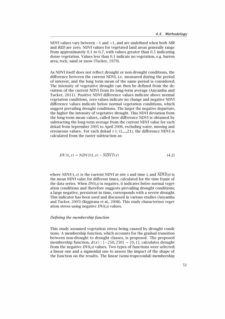
4.4. Methodology
NDVI values vary between −1 and +1, and are undefined when both NIRand RED are zero. NDVI values for vegetated land areas generally rangefrom approximately 0.1 to 0.7, with values greater than 0.5 indicatingdense vegetation. Values less than 0.1 indicate no vegetation, e.g. barrenarea, rock, sand or snow (Tucker, 1979).
As NDVI itself does not reflect drought or non-drought conditions, thedifference between the current NDVI, i.e. measured during the periodof interest, and the long term mean of the same period is considered.The intensity of vegetative drought can then be defined from the de-viation of the current NDVI from its long-term average (Anyamba andTucker, 2011). Positive NDVI difference values indicate above normalvegetation conditions, zero values indicate no change and negative NDVIdifference values indicate below normal vegetation conditions, whichsuggest prevailing drought conditions. The larger the negative departure,the higher the intensity of vegetative drought. This NDVI deviation fromthe long-term mean values, called here difference NDVI is obtained bysubtracting the long-term average from the current NDVI value for eachdekad from September 2005 to April 2006, excluding water, missing anderroneous values. For each dekad i ∈ (1,...,21), the difference NDVI iscalculated from the raster subtraction as:
DV(t, s) = NDVI(t, s)−NDVI(s) (4.2)
where NDVI(t, s) is the current NDVI at site s and time t, and NDVI (s) isthe mean NDVI value for different times, calculated for the time frame ofthe data series. When DV(t,s) is negative, it indicates below normal veget-ation conditions and therefore suggests prevailing drought conditions;a large negative, persistent in time, corresponds with a severe drought.This indicator has been used and discussed in various studies (Anyambaand Tucker, 2005) (Bajgirana et al., 2008). This study characterises veget-ation stress using negative DV(t,s) values.
Defining the membership function
This study assumed vegetation stress being caused by drought condi-tions. A membership function, which accounts for the gradual transitionbetween non-drought to drought classes, is proposed. The proposedmembership function, d(x) : [−250,250] → [0,1], calculates droughtfrom the negative DV(t,s) values. Two types of functions were selected:a linear one and a sigmoidal one to assess the impact of the shape ofthe function on the results. The linear (semi-trapezoidal) membership
51
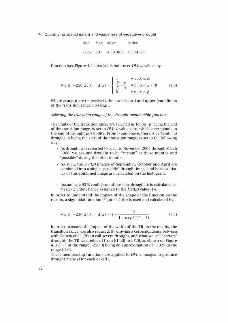
4. Quantifying spatial extent and vagueness of vegetative drought
Min Max Mean Stdev
-225 207 4.397862 9.339158
function (see Figure 4.1 (a)) d(x) is built over DV(t,s) values by:
∀x ∈ [−250,250], d(x) =
1 ∀x : x ≤ αβ− xβ−α ∀x : α < x < β
0 ∀x : x ≥ β(4.3)
Where α and β are respectively the lower (start) and upper (end) limitsof the transition range (TR) ]α,β[.
Selecting the transition range of the drought membership function
The limits of the transition range are selected as follow: β, being the endof the transition range, is set to DV(t,s) value zero, which corresponds tothe end of drought possibility. From 0 and above, there is certainly nodrought. α being the start of the transition range, is set in the followingway:
• As drought was reported to occur in November 2005 through March2006, we assume drought to be “certain” at these months and“possible” during the other months.
• As such, the DV(t,s) images of September, October and April arecombined into a single “possible” drought image and basic statist-ics of this combined image are calculated on the histogram.
• Assuming a 95 % confidence of possible drought, b is calculated as:Mean - 2 Stdev, hence assigned to the DV(t,s) value -14.
In order to understand the impact of the shape of the function on theresults, a sigmoidal function (Figure 4.1 (b)) is used and calculated by:
∀x ∈ [−250,250], d(x) = 1− 2
1+ exp(−2x3 − 5)
(4.4)
In order to assess the impact of the width of the TR on the results, thetransition range was also reduced. By drawing a correspondence betweenwith Gouvia et al. (2009) call severe drought, and what we call “certain”drought, the TR was reduced from ]-14,0[ to ]-7,0[, as shown on Figure4.1(c). -7 in the range [-250,0] being an approximation of -0.025 in therange [-1,0].These membership functions are applied to DV(t,s) images to producedrought maps D for each dekad i.
52
4.4. Methodology
Figure 4.1 (a) Linear drought membership function applied to DV(t,s) images,with the transition range TR = ] − 14,0[; (b) Sigmoidal drought membershipfunction applied to DV(t,s) images, with TR = ] − 14,0[; (c) Linear droughtmembership function applied to DV(t,s) images, with TR = ]− 7,0[.
4.4.2 Quantifying vegetative drought
Quantifying vegetative drought involves using measures adapted fromthe ones proposed by Dilo (2006); Dilo et al. (2007b,a) for continuousspace. These measures are modified for raster images. Visualising theevolution of vegetative drought area in space and time is done using atracking software developed by (Turdukulov et al., 2005) and modifiedto use the proposed measures. The following sections paragraphs details.
Vegetative drought measures
The measures proposed to quantify drought are: the total size of theareas possibly covered by drought, called total-area; the total size ofthe areas certainly covered by drought, called the core-area; and anaverage of the area sizes of drought with the different certainty degrees,called mean-area. This study also quantify the degree of uncertainty
53
4. Quantifying spatial extent and vagueness of vegetative drought
of vegetative drought with a measure called vagueness. These droughtmeasures are built on measures proposed for vague objects in the con-tinuous space IR2 (Dilo, 2006; Dilo et al., 2007b,a), and are adapted toraster data. The following paragraphs detail the process of buildingthese measures.
The total-area of drought is the area size of the possible droughtlocations, i.e. locations with positive membership values. For a vagueregion µ : IR2 → [0,1], the total area is Area (
{(x,y) ∈ IR2|µ(x,y) > 0
}).
The data composed of raster images, Di for each dekad, which areproduced from the data processing of the previous step. In the followingequations we use D to notate the set of pixels in the image, and d(j) toindicate the value of drought in pixel j. The D total-area is calculatedby:
total-area =∑
{j∈D|d(j)>0}pixel-size (4.5)
Thus, the total-area is equal to the pixel size multiplied by the numberof positive pixels.
The core-area is the area size of the certain drought locations. Vegetativedrought can be described in different levels of certainty using the conceptof α-cuts (Klir and Yuan, 1995): µα =
{(x,y) ∈ IR2|µ(x,y) ≥ α
}, where
α ∈]0,1]. The certain drought region is the 1-cut, which area size is thecore-area:Area(
{(x,y) ∈ IR2|µ(x,y) = 1
}). For a raster image D, the core-area is
calculated by:
core-area =∑
{j∈D|d(j)=1}pixel-size (4.6)
Thus, the core-area of drought is equal to the pixel-size multiplied bythe number of 1-valued pixels in D.
The different α-cuts produce different description of drought, each asso-ciated with a different certainty level, α. To get an estimation of the areasize that accounts for all the different descriptions based on α-cut values,the study calculates the arithmetic mean of area sizes of α-cuts. Thismeasure is the mean-area. For a vague region µ in IR2 the mean-area(µ)is equal to
∫∫µ(x,y)dx dy Dilo et al. (2007a,b); Dilo (2006). For a raster
image D, the mean-area is calculated by replacing the integral with thesum:
mean-area =∑{j∈D}
d(j) · pixel-size (4.7)
54
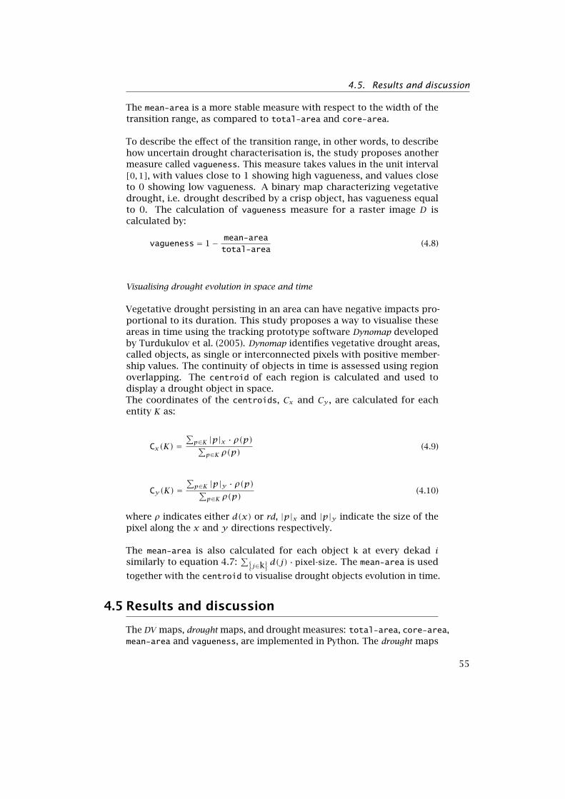
4.5. Results and discussion
The mean-area is a more stable measure with respect to the width of thetransition range, as compared to total-area and core-area.
To describe the effect of the transition range, in other words, to describehow uncertain drought characterisation is, the study proposes anothermeasure called vagueness. This measure takes values in the unit interval[0,1], with values close to 1 showing high vagueness, and values closeto 0 showing low vagueness. A binary map characterizing vegetativedrought, i.e. drought described by a crisp object, has vagueness equalto 0. The calculation of vagueness measure for a raster image D iscalculated by:
vagueness = 1− mean-area
total-area(4.8)
Visualising drought evolution in space and time
Vegetative drought persisting in an area can have negative impacts pro-portional to its duration. This study proposes a way to visualise theseareas in time using the tracking prototype software Dynomap developedby Turdukulov et al. (2005). Dynomap identifies vegetative drought areas,called objects, as single or interconnected pixels with positive member-ship values. The continuity of objects in time is assessed using regionoverlapping. The centroid of each region is calculated and used todisplay a drought object in space.The coordinates of the centroids, Cx and Cy , are calculated for eachentity K as:
Cx(K) =∑p∈K |p|x · ρ(p)∑
p∈K ρ(p)(4.9)
Cy(K) =∑p∈K |p|y · ρ(p)∑
p∈K ρ(p)(4.10)
where ρ indicates either d(x) or rd, |p|x and |p|y indicate the size of thepixel along the x and y directions respectively.
The mean-area is also calculated for each object k at every dekad isimilarly to equation 4.7:
∑{j∈k
} d(j) · pixel-size. The mean-area is used
together with the centroid to visualise drought objects evolution in time.
4.5 Results and discussion
The DV maps, drought maps, and drought measures: total-area, core-area,mean-area and vagueness, are implemented in Python. The drought maps
55
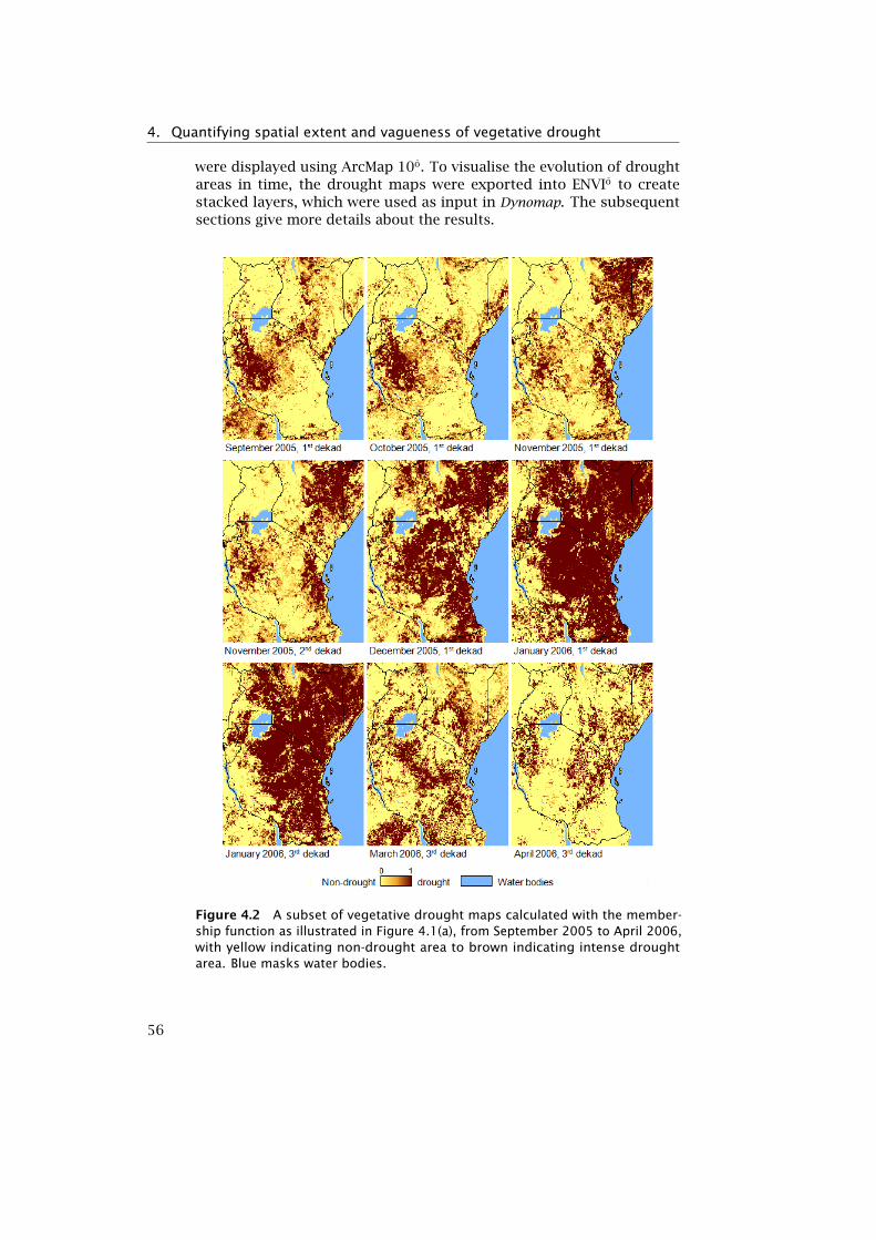
4. Quantifying spatial extent and vagueness of vegetative drought
were displayed using ArcMap 10o. To visualise the evolution of droughtareas in time, the drought maps were exported into ENVIo to createstacked layers, which were used as input in Dynomap. The subsequentsections give more details about the results.
Figure 4.2 A subset of vegetative drought maps calculated with the member-ship function as illustrated in Figure 4.1(a), from September 2005 to April 2006,with yellow indicating non-drought area to brown indicating intense droughtarea. Blue masks water bodies.
56
4.5. Results and discussion
4.5.1 Characterising vegetative drought with vague maps
A subset of drought maps is shown in Figure 4.2. Yellow indicates non-drought areas, i.e. with a drought membership value equal to 0, andbrown indicates severe drought areas, i.e. with a drought membershipvalue equal to 1. Blue indicates water bodies and black lines countries’boundaries (refer to Figure 1.6).
Looking at the maps in Figure 4.2, one observes a moderate drought af-fected area from the first dekad of September through October. Droughtintensified in the region, as indicated by an increase of brown pixels,from the second dekad of November through January. This intensitydecreased in February throughout April, as indicated with a decrease ofbrown pixels.
Figure 4.3 Averaged monthly rainfall anomaly (difference with the long term)from September 2005 to April 2006 for Kenya and Tanzania.
As no ground collected data on vegetation conditions were availableto validate the results, the trend of drought evolution observed in theresults were compared with rainfall anomaly (see Figure 4.3) calculatedfor Kenya and Tanzania, which are the two main countries making upthe study area.
Daily rainfall data for Kenya, and Tanzania from September 2005 toApril 2006 were acquired from the National Climatic Data Center 4. Themonthly long-term rainfall data, for the same stations in these countriesand covering the same period, were acquired from the World Meteoro-logical Organization. Monthly rainfall anomaly was calculated for eachstation and averaged by country. Figure 4.3 shows the deviation of thecurrent (September 2005 to April 2006) amount of rainfall from the cor-responding long-term average, considered as normal. 0 values indicatenormal amount of rainfall, negative values indicate below normal amount
4http://gis.ncdc.noaa.gov/geoportal/catalog/main/home.page
57
4. Quantifying spatial extent and vagueness of vegetative drought
of rainfall and positive values indicate above normal amount of rainfall.
Figure 4.3 shows a below average condition of rainfall from October 2005through February 2006, with a severe lack of rainfall occurring betweenNovember and February, as for drought (Figure 4.2). The lack of rainfallobserved in October 2005 worsened through December and can explainthe level of drought intensification observed in January 2006. In April2006 drought conditions started fading. This can be explained by theslow return to normal rainfall condition observed in March.
4.5.2 Quantifying vegetative drought
Vegetative drought area for the region is measured using the total-area,core-area, and the mean-area. Figure 4.4 shows the areas, expressed inkm2, calculated per dekad and plotted against each other.In all figures, the total-area remains the same as the same end for theTR, 0, was used. These values vary between a minimum of 656 448km2 and a maximum of 1 870 080 km2. The core-area values does notsignificantly change after changing the shape of the function, however itchanges drastically after reducing the transition range, and affects themean ares in Figure 4.4(c). In Figures 4.4(a) and 4.4(b), the core-areavaries between a minimum of 60 096 km2 and a maximum of 1 424 448km2, while in Figure 4.4(c) it varies between 296 640 km2 and 1 647 104km2. The mean-area varies between a minimum of 358 560 km2 and amaximum of 1 637 344 km2 in Figures 4.4(a) and 4.4(b), while it variesbetween 502 198 km2 and 1 756 525 km2 in 4.4(c).
With the difference of the core-area minimum values being 236 544km2, and of the mean-area minimum values being 143 636 km2, it canbe concluded that the mean-area measure is more stable measure ofvegetative drought area, i.e. its values are less affected from the changeof TR than the core.
The difference between the total-area and the core-area values varyfor each dekad. The magnitude of this difference is reduced in Figure4.4(c), as the transition range was reduced. In all the cases though, thedifference remains higher at the beginning of drought than at the end,and was the smallest at the peak of the drought event in January 2006.This variation shows that vegetative drought is more spatially vague atits beginning than at its end, and less vague at its peak.
The degree of vagueness of vegetative drought characterisation is alsoquantified. This uncertainty is quantified using the vagueness measure,as shown in figure 4.5.
The degree of vagueness of vegetative drought is plotted for all thedekads, for both TR. By defining the severity of vegetative drought
58
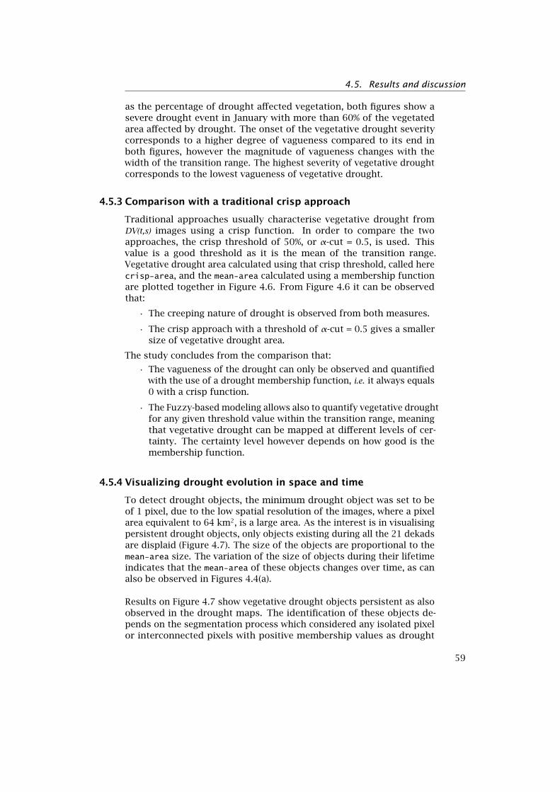
4.5. Results and discussion
as the percentage of drought affected vegetation, both figures show asevere drought event in January with more than 60% of the vegetatedarea affected by drought. The onset of the vegetative drought severitycorresponds to a higher degree of vagueness compared to its end inboth figures, however the magnitude of vagueness changes with thewidth of the transition range. The highest severity of vegetative droughtcorresponds to the lowest vagueness of vegetative drought.
4.5.3 Comparison with a traditional crisp approach
Traditional approaches usually characterise vegetative drought fromDV(t,s) images using a crisp function. In order to compare the twoapproaches, the crisp threshold of 50%, or α-cut = 0.5, is used. Thisvalue is a good threshold as it is the mean of the transition range.Vegetative drought area calculated using that crisp threshold, called herecrisp-area, and the mean-area calculated using a membership functionare plotted together in Figure 4.6. From Figure 4.6 it can be observedthat:
• The creeping nature of drought is observed from both measures.
• The crisp approach with a threshold of α-cut = 0.5 gives a smallersize of vegetative drought area.
The study concludes from the comparison that:
• The vagueness of the drought can only be observed and quantifiedwith the use of a drought membership function, i.e. it always equals0 with a crisp function.
• The Fuzzy-based modeling allows also to quantify vegetative droughtfor any given threshold value within the transition range, meaningthat vegetative drought can be mapped at different levels of cer-tainty. The certainty level however depends on how good is themembership function.
4.5.4 Visualizing drought evolution in space and time
To detect drought objects, the minimum drought object was set to beof 1 pixel, due to the low spatial resolution of the images, where a pixelarea equivalent to 64 km2, is a large area. As the interest is in visualisingpersistent drought objects, only objects existing during all the 21 dekadsare displaid (Figure 4.7). The size of the objects are proportional to themean-area size. The variation of the size of objects during their lifetimeindicates that the mean-area of these objects changes over time, as canalso be observed in Figures 4.4(a).
Results on Figure 4.7 show vegetative drought objects persistent as alsoobserved in the drought maps. The identification of these objects de-pends on the segmentation process which considered any isolated pixelor interconnected pixels with positive membership values as drought
59
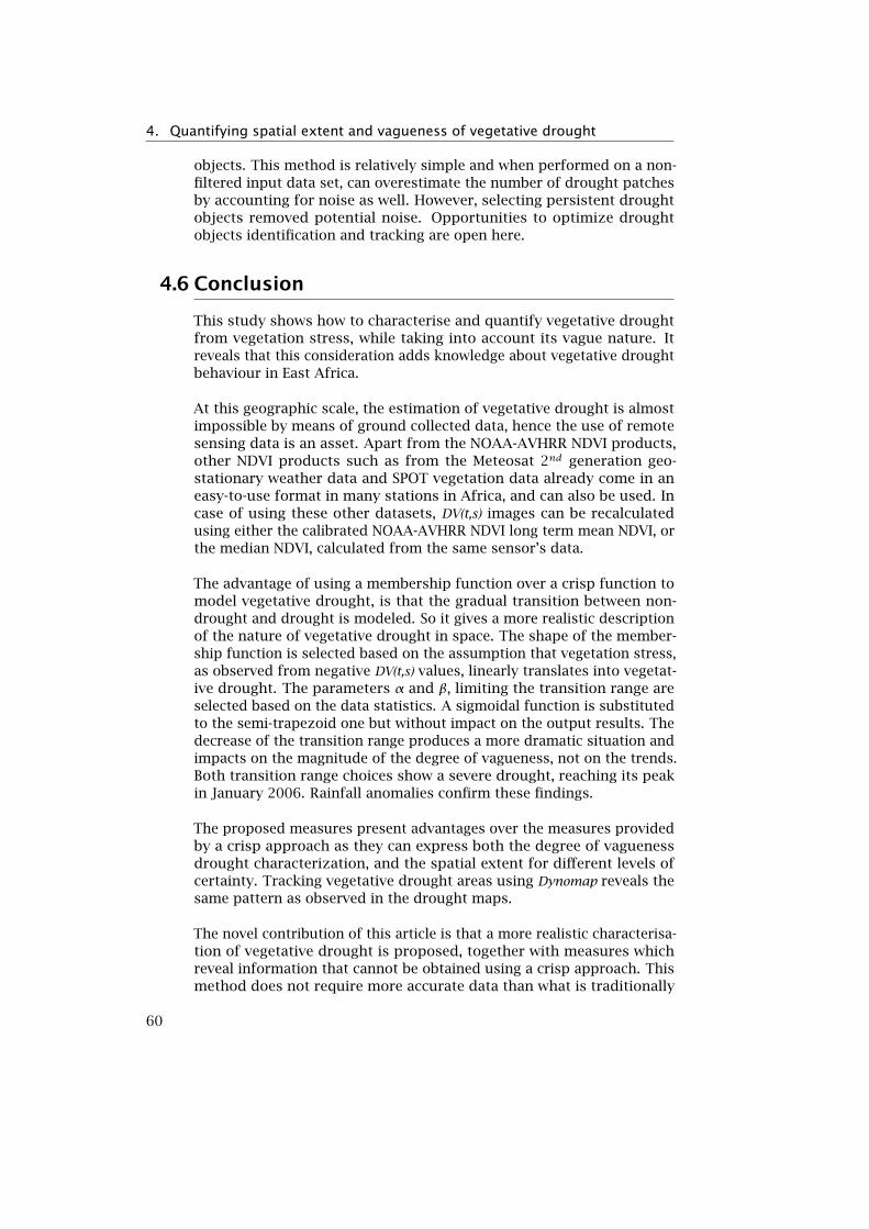
4. Quantifying spatial extent and vagueness of vegetative drought
objects. This method is relatively simple and when performed on a non-filtered input data set, can overestimate the number of drought patchesby accounting for noise as well. However, selecting persistent droughtobjects removed potential noise. Opportunities to optimize droughtobjects identification and tracking are open here.
4.6 Conclusion
This study shows how to characterise and quantify vegetative droughtfrom vegetation stress, while taking into account its vague nature. Itreveals that this consideration adds knowledge about vegetative droughtbehaviour in East Africa.
At this geographic scale, the estimation of vegetative drought is almostimpossible by means of ground collected data, hence the use of remotesensing data is an asset. Apart from the NOAA-AVHRR NDVI products,other NDVI products such as from the Meteosat 2nd generation geo-stationary weather data and SPOT vegetation data already come in aneasy-to-use format in many stations in Africa, and can also be used. Incase of using these other datasets, DV(t,s) images can be recalculatedusing either the calibrated NOAA-AVHRR NDVI long term mean NDVI, orthe median NDVI, calculated from the same sensor’s data.
The advantage of using a membership function over a crisp function tomodel vegetative drought, is that the gradual transition between non-drought and drought is modeled. So it gives a more realistic descriptionof the nature of vegetative drought in space. The shape of the member-ship function is selected based on the assumption that vegetation stress,as observed from negative DV(t,s) values, linearly translates into vegetat-ive drought. The parameters α and β, limiting the transition range areselected based on the data statistics. A sigmoidal function is substitutedto the semi-trapezoid one but without impact on the output results. Thedecrease of the transition range produces a more dramatic situation andimpacts on the magnitude of the degree of vagueness, not on the trends.Both transition range choices show a severe drought, reaching its peakin January 2006. Rainfall anomalies confirm these findings.
The proposed measures present advantages over the measures providedby a crisp approach as they can express both the degree of vaguenessdrought characterization, and the spatial extent for different levels ofcertainty. Tracking vegetative drought areas using Dynomap reveals thesame pattern as observed in the drought maps.
The novel contribution of this article is that a more realistic characterisa-tion of vegetative drought is proposed, together with measures whichreveal information that cannot be obtained using a crisp approach. Thismethod does not require more accurate data than what is traditionally
60

4.6. Conclusion
used. The method is generic in a way that it can also be applied inother regions of the World, and adapted to monitor other vague spatialphenomena such as water pollution in rivers and lakes, or air pollution.
61
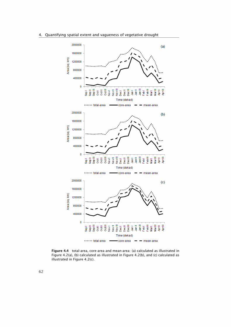
4. Quantifying spatial extent and vagueness of vegetative drought
Figure 4.4 total-area, core-area and mean-area: (a) calculated as illustrated inFigure 4.2(a), (b) calculated as illustrated in Figure 4.2(b), and (c) calculated asillustrated in Figure 4.2(c).
62
4.6. Conclusion
Figure 4.5 Degree of vagueness of vegetative drought for all dekads with TR =]−14,0[ (top image) and ]−7,0[ (bottom image), plotted against the percentageof mean-area of drought and non-drought area respectively.
63
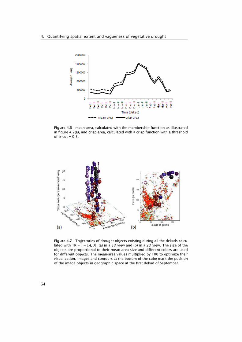
4. Quantifying spatial extent and vagueness of vegetative drought
Figure 4.6 mean-area, calculated with the membership function as illustratedin figure 4.2(a), and crisp-area, calculated with a crisp function with a thresholdof α-cut = 0.5.
Figure 4.7 Trajectories of drought objects existing during all the dekads calcu-lated with TR = ]− 14,0[; (a) in a 3D view and (b) in a 2D view. The size of theobjects are proportional to their mean-area size and different colors are usedfor different objects. The mean-area values multiplied by 100 to optimize theirvisualization. Images and contours at the bottom of the cube mark the positionof the image objects in geographic space at the first dekad of September.
64
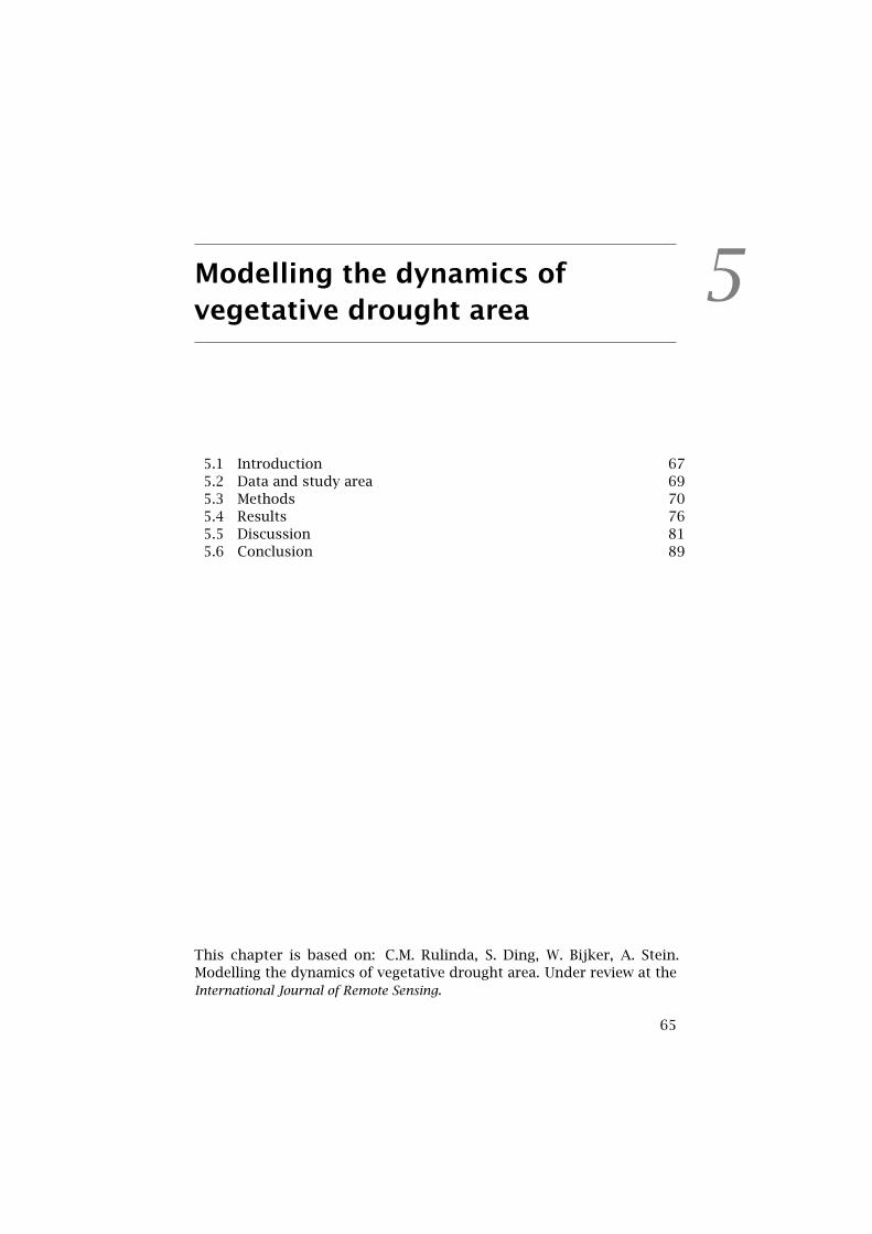
5Modelling the dynamics ofvegetative drought area
5.1 Introduction 675.2 Data and study area 695.3 Methods 705.4 Results 765.5 Discussion 815.6 Conclusion 89
This chapter is based on: C.M. Rulinda, S. Ding, W. Bijker, A. Stein.Modelling the dynamics of vegetative drought area. Under review at theInternational Journal of Remote Sensing.
65
5. Modelling the dynamics of vegetative drought area
Abstract
This chapter explores the potential to model the changes of vegetativedrought areas using NDVI data from NOAA-AVHRR. A fuzzy classificationapproach was used to model the vegetative drought classes and Markovchains were used to model the changes of areas of these classes. Themethod was implemented on the drought prone region of East Africafirst, and in Kenya, using data from March to May, and October toDecember, 1998 to 2008. Three classes were defined and probabilitytransition matrices were calculated per season and per dekad. Thetransition probability matrices showed that in East Africa there is ahigher probability (p � 0.5) to remain or change to the “normal” classfrom either “dry” or “wet” classes. Using the same method, in Kenyathere is a higher probability to remain “wet”. The transition matriceswere further used to predict the areas of the classes. The “normal”class was predicted with less error (mean absolute error = 0.01). ForEast Africa, values were predicted with less errors than in Kenya andthe dekadal matrices perform better than the seasonal matrices. Theproposed method offers for the first time a possibility to quantitativelyassess the dynamics of the area of vegetative drought at a regional level.
66
5.1. Introduction
5.1 Introduction
Drought is a vague concept as it has meanings from different perspect-ives. It can be defined as a natural but temporary water scarcity thatcan have a substantial impact on the ecosystem and agriculture of theaffected region. The prime cause of drought is the occurrence of be-low normal precipitation, which in turn, is caused by various naturalphenomena (Panu and Sharma, 2002). The amount of drought causedby precipitation shortfalls varies according to local topography, soilsand vulnerability. For instance, in areas where most of the vegetationdepends on rainfall, the direct impact of drought is the damage to plants,that usually results in losses of crops and pastures, while in other areasplants might be less affected or not at all. Vegetative drought in thisstudy is associated with the short-term effects of precipitation shortfallson plants in general.
A combination of droughts, or a sequence of droughts, with humanactivities may lead to desertification of vulnerable arid, semi-arid anddry subhumid areas, whereby, soil structure and soil fertility degradeand bio-productive resources decrease or disappear (Kundzewicz, 1997).In East Africa for instance, recurring droughts leading to desertificationhave created grave ecological catastrophes, prompting massive foodshortages in certain areas (Pantuliano and Pavanello, 2009).
Unlike desertification, management of vegetation stress as a consequenceof precipitation shortfalls requires the development and implementationof preparedness and emergency measures to reduce the adverse effectsand minimize for instance crop losses. In this context, preparedness,prediction and early warning system are necessary (Paulo and Ferreira,2007; Pereira et al., 2009). Understanding and predicting the dynam-ics of drought can therefore improve the development of preparadnessmeasures. The lack of clearly agreed definitions and knowledge on theprobability of drought occurences, however, makes it difficult to ad-equately evaluate the impacts and to implement preparedness measureswhen a drought occurs (Rojas et al., 2011).
Considerable efforts to model the dynamics of droughts using stochasticmodels have been made; some references to related studies can be foundin Mishra and Desai (2005). Most of these efforts are focused on meteoro-logical droughts, where Markov chains proved to be useful to predict thechanges of drought classes (Paulo et al., 2005; Paulo and Ferreira, 2007).The Markov chain model is named after the Russian mathematician An-drei Andreevich Markov (1856-1922), who developed the Markov chainas a natural extension of sequences of independent random variables. AMarkov process usually refers to a first-order process of auto-regressiveprocesses. The future development of this process is completely determ-ined by the present state and is independent of the way in which the
67
5. Modelling the dynamics of vegetative drought area
present state has developed, which explains the “first-order” (Chatfield,2004). A Markov chain is a discrete-state random process of a Markovprocess and it is a simple linear model (Meyn and Tweedie, 1993; Sinclair,2005). A Markov chain is also a special case of a Markov process, whichitself is a special case of a random or stochastic process. Mishra and De-sai (2009) combined Joint probability Density Function and Markov chainprocess to characterize drought with SPI. Banik et al. (2002) modeledweekly rainfall data by Markov chain and the results illustrated a betterunderstanding of drought-proneness and identification of the areas for along-term drought mitigation. Paulo and Ferreira (2007) used SPI valuesof 67 years of rainfall data into Markov chain to predict hydrologicaldrought. Results showed that the Markov chain approach applied totime series is proved to be a useful tool to understand the stochasticcharacteristics of drought and for early warning system. Markov chainswere also used for non-drought studies, such as in Balzter (2000) whoused four different locations with different climatic and soil conditionsto examine different grassland species. Results show that Markov chainmodels are sensitive to changes and information from models is valuablefor conservation, land planning and ecology. Compared to regressionvariables in crop field forecasting, the Markov chain proved to be anattractive alternative to regression analysis, because the approach isnon-parametric, simple to implement with Markov property as the onlyrequirement (Matis et al., 1985). In a recent study by Ding et al. (2011),Markov chains have been used to model the dekadal dynamics of vegetat-ive drought classes modelled as vague classes using the fuzzy set theory,for 20 pixels individually. The method showed a potential to predict thefuture vegetative drought class of a pixel on a dekadal basis.
Fuzzy sets were first introduced by Zadeh (1965, 1968, 1984) as an exten-sion of the classical set theory. In classical set theory, the membershipof elements in a set is assessed in binary terms according to a bivalentcondition with only two values: 0 and 1. In fuzzy set theory, classicalbivalent sets are usually called crisp sets. By contrast, fuzzy set theorypermits the gradual assessment of the membership of elements in a set.Each fuzzy set is bounded by transition ranges. A fuzzy membershipfunctions µA(x) has often been regarded as a compatibility function,which denotes the degree in which the proposition “x is A” is true (Drako-poulos, 1995). To define a fuzzy set, values of threshold, dispersionand selection of appropriate membership function are required. Thereare different types of membership functions. Common examples areBoolean, bell-shaped, triangular, Gaussian and trapezoidal. Values ofthreshold can be selected using statistical methods or based on fieldknowledge. In this study, the dynamics of vegetative drought areas aremodeled using Markov chains applied to traingular and trapezoidal fuzzyclasses. In previously mentioned studies, drought classes are modeledas crisp classes. Some authors have developed the concepts of fuzzyMarkov chains, where Markov chains are applied to fuzzy classes orstates. Dilo (2006) used fuzzy Markov chains to model beach erosion
68
5.2. Data and study area
with the ratio of average area. Miao et al. (2005) predicted the futurevalue of cultivated land demand in land use planning using traditionalhomogeneous Markov chains model with fuzzy probabilities. Resultsproved that the accuracy of prediction is improved with fuzzy set theory.
The present work is a continuation of the study by Ding et al. (2011),where a group of homogeneous pixels, called area, is considered insteadof individual pixels. The aim of this study is to explore the potentialof Markov chains for the modelling of dynamics of areas of vegetativedrought at a regional level. The method is applied on the drought proneregion of Eastern Africa.
5.2 Data and study area
5.2.1 Data
A drought variable is responsible for assessing drought effects, and isconsidered a key element in defining drought and deciding on techniquesfor its analysis (Panu and Sharma, 2002). For vegetative drought, theNormalized Difference Vegetation Index (NDVI) is used as an indicator ofvegetation status (Tucker, 1979). The 10-days (dekadal) NOAA-AVHRRNDVI images freely available from the FEWSNET (FEWSNETd, 2005) web-site are used as input. Images covering the two rainy seasons in EastAfrica from 1998 to 2008 are considered. The first season lasts fromMarch to May, and the second one from October to December. The pixelsize is 8 km. The 11 years period is selected as the minimum to capturethe dynamics of vegetative drought, knowing that in most of these yearsthe region experiences drought episodes.
The study applied the Global Land Cover map 2000 (GLC2000) mask(EC-JRC-GEMU, 2000) to exclude non-vegetation classes and vegetationclasses such as forests, swamps and irrigated vegetation. Forests’ classeswere not of interest as they are generally more resilient to precipitationshortfalls and forest drought will have only short term effect on the live-lihoods of the land users. Swamp areas, being on wetland, are expectedto respond differently to drought conditions, and irrigated crops aremore influenced by human activities.
5.2.2 Study area
The study area covers a subset of East Africa as seen on Figure 1.6.The region, also referred to as the Great Lakes region of East Africa, issituated between 5◦ 30” N, 12◦ S, and 28◦ 45” E and 41◦ 50” E. Thesecountries together, currently forming the East Africa Community (EAC),cover a surface of 1.72 million Km2, excluding water, with a populationof more than 133.5 million (EAC, 2010). The climate in the region isdiverse, but predominantly semi-arid. Agriculture is one of the region’s
69
5. Modelling the dynamics of vegetative drought area
most important sectors, with about 80 % of the population of the EastAfrican community partner states living in rural areas and depending onagriculture for their livelihood.
East Africa is a drought prone region at high risk of food insecurity(FEWSNETb, 2011). In general, the growing seasons follow the rainy sea-sons and vegetation dynamics is highly dependent on rainfall (Davenportand Nickolson, 1993). There are two rainy seasons, an abundant rainyseason from March to May and a less abundant season from Octoberto December. Crops and animal pasture are renewed during the rainyseasons. Large precipitation shortfalls in the past decade cause periodicdrought episodes in the region (FEWSNETb, 2011).
The proposed method was also applied to Kenya, covering an area of581 000 km2 excluding water (Figure 1.6). Kenya has been prone todrought episodes in the last dekades, especially in the North wheresevere droughts have led to famine, displacement and death.
5.3 Methods
5.3.1 Vegetative drought parameters
As NDVI itself cannot indicate drought, the study used the NDVI anomalyDV(t,s), calculated per pixel by Equation (5.1), as an indicator of vegetativedrought (Anyamba and Tucker, 2011), (Thenkabail et al., 2004), (Muradand Islam Saiful, 2011). A time series of DV(t,s) images provide there-fore the framework for evaluating the vegetative drought parameters ofinterest.
DV(t, s) = NDVI(t, s)−NDVI(s) (5.1)
where NDVI(t, s) is the current NDVI at site s and time t, and NDVI (s) is themean NDVI value for different times, calculated for the time frame of thedata series. When DV(t,s) is negative, it indicates below normal vegetationconditions and therefore suggests prevailing drought conditions; a largenegative, persistent in time, corresponds with a severe drought.
Important parameters to quantify drought are its duration, its severity,where and when does it occur, and its areal coverage. Also, the ratioof severity to duration, called magnitude or intensity, is used (Dracupet al., 1980). The basic element for deriving the above parameters isthe truncation or the threshold x0 level (Dracup et al., 1980), definedas in equation (5.2). For a pixel over time, xm, s, and cv are the mean,standard deviation and the coefficient of variation of the time series of
70
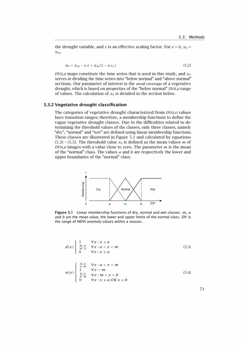
5.3. Methods
the drought variable, and e is an effective scaling factor. For e = 0, x0 =xm.
x0 = xm − e.s = xm(1− e.cv) (5.2)
DV(t,s) maps constitute the time series that is used in this study, and x0
serves at dividing the time series into “below normal” and “above normal”sections. Our parameter of interest is the areal coverage of a vegetativedrought, which is based on properties of the “below normal” DV(t,s) rangeof values. The calculation of x0 is detailed in the section below.
5.3.2 Vegetative drought classification
The categories of vegetative drought characterized from DV(t,s) valueshave transition ranges; therefore, a membership functions to define thevague vegetative drought classes. Due to the difficulties related to de-termining the threshold values of the classes, only three classes, namely“dry”, “normal” and “wet” are defined using linear membership functions.These classes are illustrated in Figure 5.1 and calculated by equations(5.3) – (5.5). The threshold value x0 is defined as the mean values m ofDV(t,s) images with a value close to zero. The parameter m is the meanof the “normal” class. The values a and b are respectively the lower andupper boundaries of the “normal” class.
Figure 5.1 Linear membership functions of dry, normal and wet classes. m, aand b are the mean value, the lower and upper limits of the normal class. DV isthe range of NDVI anomaly values within a season.
d(x)
1 ∀x : x ≤ am−xm−a ∀x : a < x <m0 ∀x : x ≥ a
(5.3)
n(x)
a−xa−m ∀x : a < x <m1 ∀x =mb−xb−m ∀x :m < x < b0 ∀x : x ≤ a OR x ≥ b
(5.4)
71
5. Modelling the dynamics of vegetative drought area
w(x)
0 ∀x : x ≤mm−xm−b ∀x :m < x < b1 ∀x : x ≥ b
(5.5)
Values for m, a and b, are determined from the statistics of dekadalDV(t,s) images. The study assumes the long-term mean NDVI imagesvalues being the normal values for each dekad, and as such, a DV(t,s)mean value of 0 means normal. The study considers K images duringthe rainy seasons of the k years, each covering a decade of days, calleddekadal images. Assuming at least one normal situation in the k years ofthe time series, the following was performed:
1 For each dekadal DV(t,s) image, the meanmd and standard deviationsd values were calculated;
2 The time series obtained in step 1 was divided into two seasons:season 1 from March to May, and season 2 from October to Decem-ber;
3 For each time series, the image of the year with the image md
value closest to 0 was selected. This step produced a time series ofdekadal images with mean values close to 0;
4 For each seasonal time series obtained in step 3, an average seasonalimage (Si), i = 1,2; its mean ms and standard deviation ss werecalculated.
The parameters ms , a and b were calculated by equations (5.6) usingSi images. ms(Si) and s(Si) are respectively the mean and standarddeviation values of the Si image.
m =m(Si)a =m(Si)− 2s(Si)b =m(Si)+ 2s(Si)
(5.6)
where m(Si) = ms and s(Si) = ss . These parameters are used in equations5.3, 5.4 and 5.5 to produce a total of k ·K · C images per season, whereC is the number of classes (C = 3). k is the number of years in the timeseries, K is the number of dekads in a season. In this study, for eachseason 297 images are produced.
5.3.3 Modeling the dynamics of the area of vegetative drought
The changes of vegetative drought classes are modelled using Markovchains that are applied to homogenous group of pixels called area. Asthe classes are defined using membership functions, the area of a classaccounts for all the pixels having positive class membership values. Thefollowing subsections detail the modelling method using Markov chains.
72
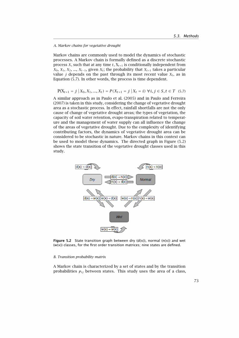
5.3. Methods
A. Markov chains for vegetative drought
Markov chains are commonly used to model the dynamics of stochasticprocesses. A Markov chain is formally defined as a discrete stochasticprocess X, such that at any time t, Xt+1 is conditionally independent fromX0, X1, X2, ..., Xt−1, given Xt ; the probability that Xt+1 takes a particularvalue j depends on the past through its most recent value Xt , as inEquation (5.7). In other words, the process is time dependent.
P(Xt+1 = j∣∣X0, X1, ..., Xt) = P(Xt+1 = j
∣∣Xt = i) ∀i, j ∈ S, t ∈ T (5.7)
A similar approach as in Paulo et al. (2005) and in Paulo and Ferreira(2007) is taken in this study, considering the change of vegetative droughtarea as a stochastic process. In effect, rainfall shortfalls are not the onlycause of change of vegetative drought areas; the types of vegetation, thecapacity of soil water retention, evapo-transpiration related to temperat-ure and the management of water supply can all influence the changeof the areas of vegetative drought. Due to the complexity of identifyingcontributing factors, the dynamics of vegetative drought area can beconsidered to be stochastic in nature. Markov chains in this context canbe used to model these dynamics. The directed graph in Figure (5.2)shows the state transition of the vegetative drought classes used in thisstudy.
Figure 5.2 State transition graph between dry (d(x)), normal (n(x)) and wet(w(x)) classes, for the first order transition matrices; nine states are defined.
B. Transition probability matrix
A Markov chain is characterized by a set of states and by the transitionprobabilities pij between states. This study uses the area of a class,
73
5. Modelling the dynamics of vegetative drought area
denoted ω and calculated here as the sum of pixels x with positive classµ membership values (Equation 5.8), to calculate these probabilities. T isthe number of pixels with positive class membership values in an image.
ωt =T∑i=1
xµ,t|xµ,t > 0 (5.8)
where ωt is the class area at time t and xµ,t is a pixel with a positive classmembership value at time t.
The transition probability pij is the element of the transition probabilitymatrix P where the Markov chain is at the next dekad t+1 in state j, giventhat it is at the present dekad t in state i. It is given by equation (5.9)
P = [pij] (5.9)
where
pij =nij∑j nij
≥ 0,∑jpij = 1 (5.10)
and nij is the total number of pixels (i.e area) in a dekadal image passingfrom class i at time t to class j at time t + 1.
In the present study, the transition probabilities are estimated per seasonby Equation (5.11), based on the area of the different classes for thewhole time series. The class transition probabilities are calculated forthe season as the average of the transition probabilities in consecutivedekads for each season.
pij =p(1,2)ij + p(2,3)ij + · · · + p(K−1,K)
ij
(K − 1)(5.11)
where K is the number of dekads in a season.These transition probabilities with the finite number of states are put
in the 3× 3 matrix P modelling the changes of vegetative drought areas.
P =
pd(x)d(x) pd(x)n(x) pd(x)w(x)
pn(x)d(x) pn(x)n(x) pn(x)w(x)
pw(x)d(x) pw(x)n(x) pw(x)w(x)
To use Markov chain for predicting the changes of vegetative droughtarea, one needs to test that the transition probabilities are time depend-ent, as in equation 5.7. In a homogenous formulation, the seasonal
74
5.3. Methods
transition probability matrix is stationary over time, hence the powern of the matrix, Pn, can be used to predict at time t+n, independentlyof n; n being the number of time steps. If the transition probabilitymatrix is not stationary through time, Tan and Yilmaz (2002) suggestedthat the Markov chain will have no predictive power. The tests of timehomogeneity and time dependence are explained in sections below.
C. Testing time homogeneity
Tests of time homogeneity are performed to determine whether theseasonal transition probability matrices are stationary over time. Foreach season, the test is implemented by dividing the entire sample periodinto M sub-periods and comparing the M first order transition probabilitymatrices with the first order seasonal transition matrix. The comparisonis performed using both the LR and Pearson χ2-tests, respectively givenby equations (5.12) and (5.13):
LR(M) = 2M∑m=1
N∑i=1
∑j∈Ci|m
nij|m logpij|mpij
∼ χ2(N∑i=1
(ci − 1)(di − 1)) (5.12)
Q(M) =M∑m=1
N∑i=1
∑j∈Ci|m
nij|m(pij|m − pij)2
pij∼ χ2(
N∑i=1
(ci − 1)(di − 1)) (5.13)
where N is the number of drought classes at time t − 1; j=1,2,3 at time t,pij|m is the transition probability of the sub-sample m; M is the numberof sub-samples. nij|m is the number of pixels passing from class i toclass j for the sub-sample m. ci is the number of elements in Ci and di isthe number of sub-periods for which a positive number of observationsis available for the ith row. Both of the tests have an asymptotic χ2
distribution with degree of freedom (df ) equal to the number of addi-tional independent restrictions imposed by the null hypothesis H0 ascompared to the alternative hypothesis Ha. For each sub-period m test,the df = N(N−1), LRprob and Qprob are respectively the probability ofLR test and Q test under df (Anderson and Goodman, 1957).
In this study, the sample is divided into dekadal transitionsM ∈ {1,2,3,4,5,6,7,8} within a season.
D. Testing time dependence
Tests of time dependence are performed to test that the process isdependent on the past, i.e. do not constitute a random walk. The studytests the null hypothesis H0 that the Markov chain is of order 0 againstthe alternative hypothesis Ha that the Markov chain is of order 1. If thishypothesis cannot be rejected, then the order is 0. If the hypothesis isrejected, then the transition probabilities are time dependent. In order
75
5. Modelling the dynamics of vegetative drought area
to test the time dependence of the Markov chains for the order 0, underH0 : ∀pij = pj (i, j = 1,2,3) Ha : ∃i : pij ≠ pj , α = 0.05 where pj =
njn ,
nj =∑nj(t). The LR and Pearson χ2 tests are performed as in equations
(5.14) and (5.15) (Bickenbach and Bode, 2003).
LR(O)(0) = 2N∑i=1
∑j∈Ci
nij(t) log(pijpj) ∼ χ2((N − 1)2) (5.14)
Q(O)(0) =N∑i=1
∑j=1
ni(t − 1)(pij − pj)2
pj∼ χ2((N − 1)2) (5.15)
where, ni(t − 1) =∑j nij(t), Ci = j : pij > 0
If the null hypothesis H0 is rejected, the Markov chains is time dependent.
5.3.4 Prediction and validation
For each image at time t+1, the estimated probability transition matrixP of the season can be multiplied by the initial distribution vector ofclasses’ area at time t to forecast the classes’ area at time t+1.
f(x)t+1 = f(x)t · P (5.16)
where f(x)t is the vector of probability distribution of areas at time t.For every dekad, predicted values xp are compared with the actual valuesusing the absolute error ε, given by equation (5.17). The absolute errorcompared predicted value and actual value xr by giving the differencebetween them.
ε =∣∣∣xp − xr∣∣∣ (5.17)
And for every season, the mean absolute error λ given by equation (5.18)is calculated.
λ =∑ni=1 εin
(5.18)
where n is the number of transitions in a season, n = K − 1.The actual values are calculated using the same procedures detailed insection (5.3.2).
5.4 Results
The pre-processing steps involved masking out classes of non-interest.Referring to the GLC2000 Africa-v5-legend, the following classes contain-ing croplands are selected: (7) mosaic forest/croplands, (18) croplands
76
5.4. Results
(>50 %), and (19) Croplands with open woody vegetation. In section 5.4.1,results of the classification process are presented and in section 5.4.2,the estimated transition probability matrices are presented. The resultsof the tests of time homogeneity and time independences are presentedin section 5.4.3, and of the sensitivity analysis in section 5.4.4. Finally,predicted and validation results are presented in section 5.4.5.
5.4.1 Vegetative drought classification
For the East African region, the estimated parameters m, a and a for the2 seasons are shown in Table (5.1).
Table 5.1 The parameters m, a, and b for each season in East Africa in theupper part of the table. The mean, Stdev, the lower (L) and upper (U ) 95%confidence bounds interval of the Difference are shown in the lower part of thetable.
Label m a bSeason 1 -0.54 -39.44 38.36
Season 2 0.46 -42.20 43.02
mean -0.04 -40.82 40.69
Stdev 0.70 1.95 3.29
L -6.39 -58.35 11.08
U 6.31 -23.28 70.29
The parameters of the normal class in both seasons are quite similar.The normal image used for the first season is slighlty drier than the oneof the second season. However the difference is not significant. This canimply that any of these images can be used interchangeability. In thisstudy we use them respectively for season 1 and season 2. These valuesare used in equations (5.3), (5.4) and (5.5) to calculate drought, normaland wet images for each dekad. The areas of each vegetative droughtclass are calculated and used to calculate the transition probabilities.
5.4.2 Transition Probability Matrices
The estimated 1st order 3× 3 transition probability Matrix P1 of season1 for East Africa to model the dynamics of vegetative drought areas isgiven by:
P1 =
0.41 0.48 0.110.22 0.49 0.280.08 0.48 0.44
77
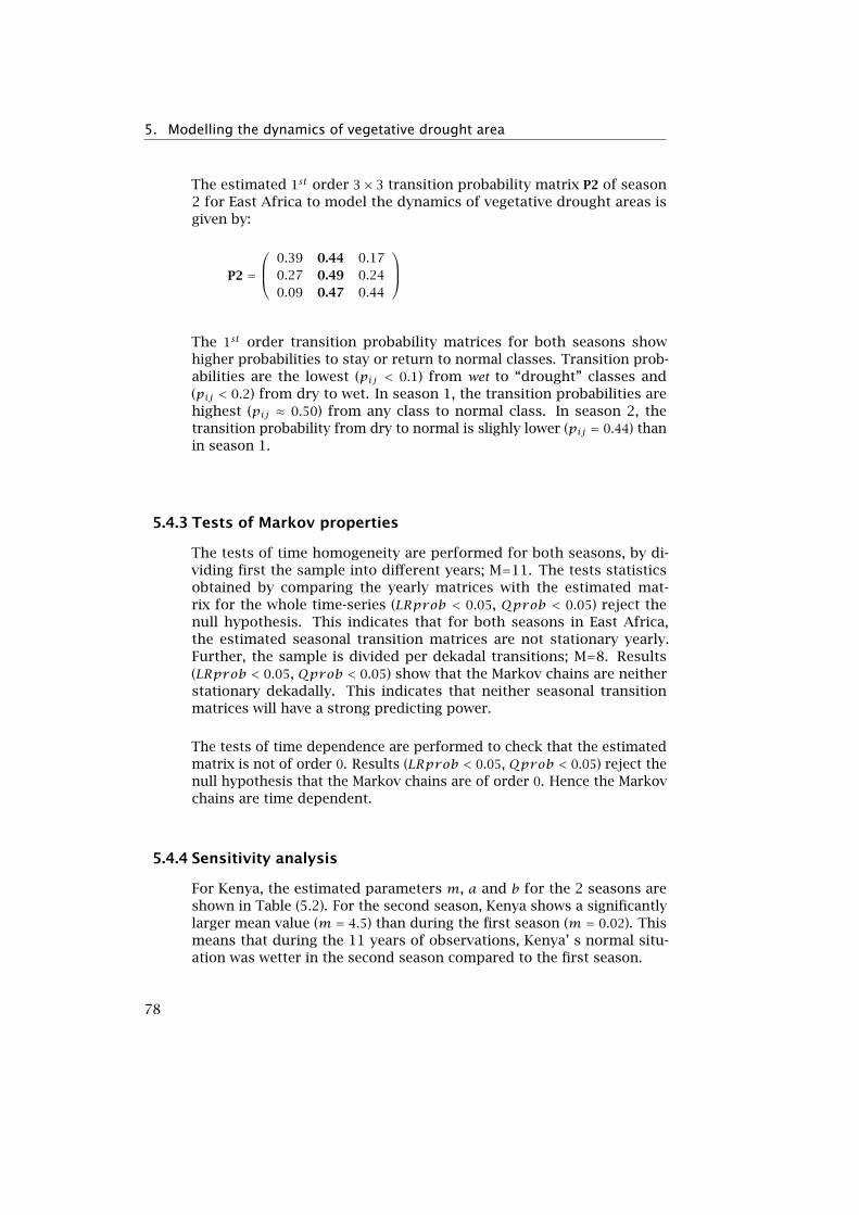
5. Modelling the dynamics of vegetative drought area
The estimated 1st order 3× 3 transition probability matrix P2 of season2 for East Africa to model the dynamics of vegetative drought areas isgiven by:
P2 =
0.39 0.44 0.170.27 0.49 0.240.09 0.47 0.44
The 1st order transition probability matrices for both seasons showhigher probabilities to stay or return to normal classes. Transition prob-abilities are the lowest (pij < 0.1) from wet to “drought” classes and(pij < 0.2) from dry to wet. In season 1, the transition probabilities arehighest (pij ≈ 0.50) from any class to normal class. In season 2, thetransition probability from dry to normal is slighly lower (pij = 0.44) thanin season 1.
5.4.3 Tests of Markov properties
The tests of time homogeneity are performed for both seasons, by di-viding first the sample into different years; M=11. The tests statisticsobtained by comparing the yearly matrices with the estimated mat-rix for the whole time-series (LRprob < 0.05, Qprob < 0.05) reject thenull hypothesis. This indicates that for both seasons in East Africa,the estimated seasonal transition matrices are not stationary yearly.Further, the sample is divided per dekadal transitions; M=8. Results(LRprob < 0.05, Qprob < 0.05) show that the Markov chains are neitherstationary dekadally. This indicates that neither seasonal transitionmatrices will have a strong predicting power.
The tests of time dependence are performed to check that the estimatedmatrix is not of order 0. Results (LRprob < 0.05, Qprob < 0.05) reject thenull hypothesis that the Markov chains are of order 0. Hence the Markovchains are time dependent.
5.4.4 Sensitivity analysis
For Kenya, the estimated parameters m, a and b for the 2 seasons areshown in Table (5.2). For the second season, Kenya shows a significantlylarger mean value (m = 4.5) than during the first season (m = 0.02). Thismeans that during the 11 years of observations, Kenya’ s normal situ-ation was wetter in the second season compared to the first season.
78
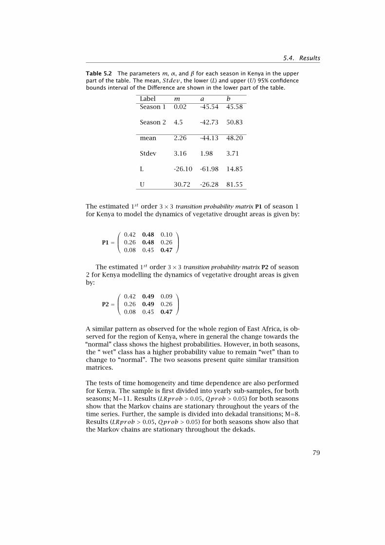
5.4. Results
Table 5.2 The parameters m, α, and β for each season in Kenya in the upperpart of the table. The mean, Stdev, the lower (L) and upper (U ) 95% confidencebounds interval of the Difference are shown in the lower part of the table.
Label m a bSeason 1 0.02 -45.54 45.58
Season 2 4.5 -42.73 50.83
mean 2.26 -44.13 48.20
Stdev 3.16 1.98 3.71
L -26.10 -61.98 14.85
U 30.72 -26.28 81.55
The estimated 1st order 3× 3 transition probability matrix P1 of season 1for Kenya to model the dynamics of vegetative drought areas is given by:
P1 =
0.42 0.48 0.100.26 0.48 0.260.08 0.45 0.47
The estimated 1st order 3× 3 transition probability matrix P2 of season
2 for Kenya modelling the dynamics of vegetative drought areas is givenby:
P2 =
0.42 0.49 0.090.26 0.49 0.260.08 0.45 0.47
A similar pattern as observed for the whole region of East Africa, is ob-served for the region of Kenya, where in general the change towards the“normal” class shows the highest probabilities. However, in both seasons,the “ wet” class has a higher probability value to remain “wet” than tochange to “normal”. The two seasons present quite similar transitionmatrices.
The tests of time homogeneity and time dependence are also performedfor Kenya. The sample is first divided into yearly sub-samples, for bothseasons; M=11. Results (LRprob > 0.05, Qprob > 0.05) for both seasonsshow that the Markov chains are stationary throughout the years of thetime series. Further, the sample is divided into dekadal transitions; M=8.Results (LRprob > 0.05, Qprob > 0.05) for both seasons show also thatthe Markov chains are stationary throughout the dekads.
79
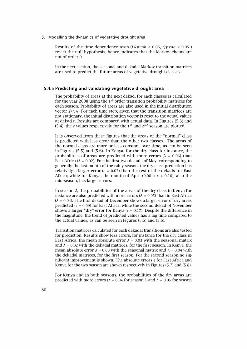
5. Modelling the dynamics of vegetative drought area
Results of the time dependence tests (LRprob < 0.05, Qprob < 0.05 )reject the null hypothesis, hence indicates that the Markov chains arenot of order 0.
In the next section, the seasonal and dekadal Markov transition matricesare used to predict the future areas of vegetative drought classes.
5.4.5 Predicting and validating vegetative drought area
The probability of areas at the next dekad, for each classes is calculatedfor the year 2008 using the 1st order transition probability matrices foreach season. Probability of areas are also used in the initial distributionvector f(x)t . For each time step, given that the transition matrices arenot stationary, the initial distribution vector is reset to the actual valuesat dekad t. Results are compared with actual data. In Figures (5.3) and(5.4), the ε values respectively for the 1st and 2nd season are plotted.
It is observed from these figures that the areas of the “normal” classis predicted with less error than the other two classes. The areas ofthe normal class are more or less constant over time, as can be seenin Figures (5.5) and (5.6). In Kenya, for the dry class for instance, theprobabilities of areas are predicted with more errors (λ = 0.06) thanEast Africa (λ = 0.02). For the first two dekads of May, corresponding togenerally the last month of the rainy season, the dry class prediction hasrelatively a larger error (ε = 0.07) than the rest of the dekads for EastAfrica; while for Kenya, the month of April (0.08 < ε < 0.10), also themid-season, has larger errors.
In season 2, the probabilities of the areas of the dry class in Kenya forinstance are also predicted with more errors (λ = 0.05) than in East Africa(λ = 0.04). The first dekad of December shows a larger error of dry areaspredicted (ε = 0.09) for East Africa, while the second dekad of Novembershows a larger “dry” error for Kenya (ε = 0.17). Despite the difference inthe magnitude, the trend of predicted values has a lag time compared tothe actual values, as can be seen in Figures (5.5) and (5.6).
Transition matrices calculated for each dekadal transitions are also testedfor prediction. Results show less errors, for instance for the dry class inEast Africa, the mean absolute error λ = 0.03 with the seasonal matrixand λ = 0.02 with the dekadal matrices, for the first season. In Kenya, themean absolute error λ = 0.06 with the seasonal matrix and λ = 0.04 withthe dekadal matrices, for the first season. For the second season no sig-nificant improvement is shown. The absolute errors ε for East Africa andKenya for the two season are shown respectively in Figures (5.7) and (5.8).
For Kenya and in both seasons, the probabilities of the dry areas arepredicted with more errors (λ = 0.04 for season 1 and λ = 0.05 for season
80
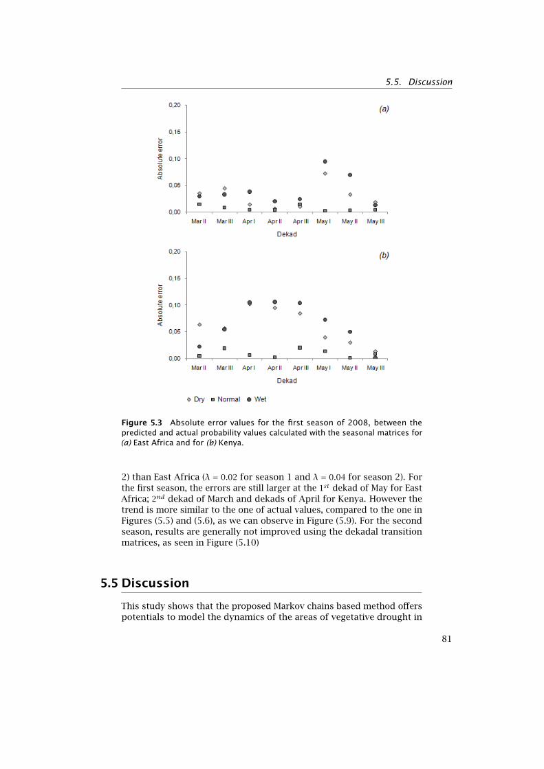
5.5. Discussion
Figure 5.3 Absolute error values for the first season of 2008, between thepredicted and actual probability values calculated with the seasonal matrices for(a) East Africa and for (b) Kenya.
2) than East Africa (λ = 0.02 for season 1 and λ = 0.04 for season 2). Forthe first season, the errors are still larger at the 1st dekad of May for EastAfrica; 2nd dekad of March and dekads of April for Kenya. However thetrend is more similar to the one of actual values, compared to the one inFigures (5.5) and (5.6), as we can observe in Figure (5.9). For the secondseason, results are generally not improved using the dekadal transitionmatrices, as seen in Figure (5.10)
5.5 Discussion
This study shows that the proposed Markov chains based method offerspotentials to model the dynamics of the areas of vegetative drought in
81
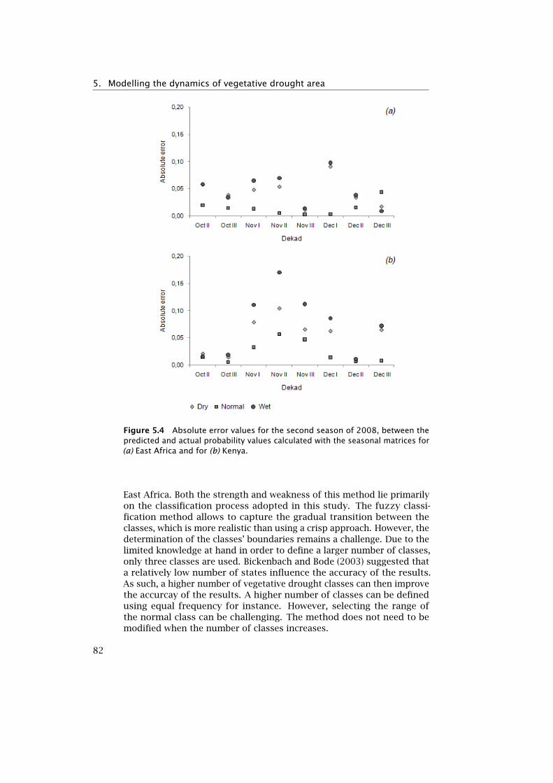
5. Modelling the dynamics of vegetative drought area
Figure 5.4 Absolute error values for the second season of 2008, between thepredicted and actual probability values calculated with the seasonal matrices for(a) East Africa and for (b) Kenya.
East Africa. Both the strength and weakness of this method lie primarilyon the classification process adopted in this study. The fuzzy classi-fication method allows to capture the gradual transition between theclasses, which is more realistic than using a crisp approach. However, thedetermination of the classes’ boundaries remains a challenge. Due to thelimited knowledge at hand in order to define a larger number of classes,only three classes are used. Bickenbach and Bode (2003) suggested thata relatively low number of states influence the accuracy of the results.As such, a higher number of vegetative drought classes can then improvethe accurcay of the results. A higher number of classes can be definedusing equal frequency for instance. However, selecting the range ofthe normal class can be challenging. The method does not need to bemodified when the number of classes increases.
82
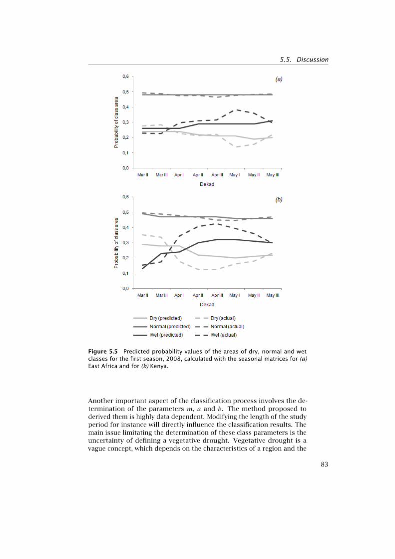
5.5. Discussion
Figure 5.5 Predicted probability values of the areas of dry, normal and wetclasses for the first season, 2008, calculated with the seasonal matrices for (a)East Africa and for (b) Kenya.
Another important aspect of the classification process involves the de-termination of the parameters m, a and b. The method proposed toderived them is highly data dependent. Modifying the length of the studyperiod for instance will directly influence the classification results. Themain issue limitating the determination of these class parameters is theuncertainty of defining a vegetative drought. Vegetative drought is avague concept, which depends on the characteristics of a region and the
83
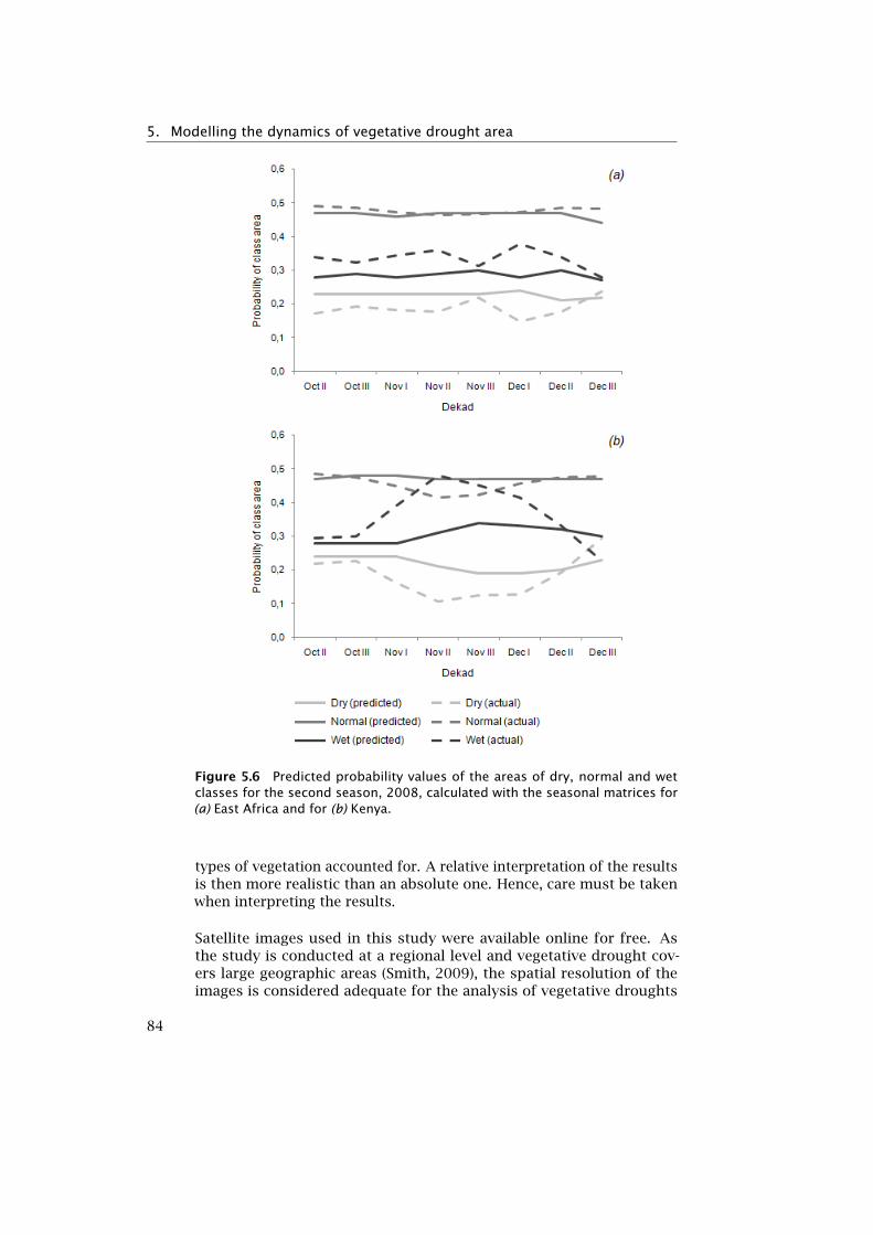
5. Modelling the dynamics of vegetative drought area
Figure 5.6 Predicted probability values of the areas of dry, normal and wetclasses for the second season, 2008, calculated with the seasonal matrices for(a) East Africa and for (b) Kenya.
types of vegetation accounted for. A relative interpretation of the resultsis then more realistic than an absolute one. Hence, care must be takenwhen interpreting the results.
Satellite images used in this study were available online for free. Asthe study is conducted at a regional level and vegetative drought cov-ers large geographic areas (Smith, 2009), the spatial resolution of theimages is considered adequate for the analysis of vegetative droughts
84
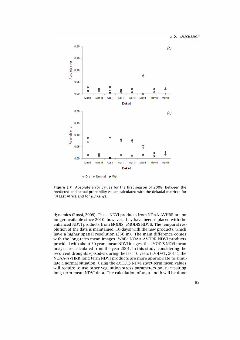
5.5. Discussion
Figure 5.7 Absolute error values for the first season of 2008, between thepredicted and actual probability values calculated with the dekadal matrices for(a) East Africa and for (b) Kenya.
dynamics (Rossi, 2009). These NDVI products from NOAA-AVHRR are nolonger available since 2010, however, they have been replaced with theenhanced NDVI products from MODIS (eMODIS NDVI). The temporal res-olution of the data is maintained (10-days) with the new products, whichhave a higher spatial resolution (250 m). The main difference comeswith the long-term mean images. While NOAA-AVHRR NDVI productsprovided with about 30 years mean NDVI images, the eMODIS NDVI meanimages are calculated from the year 2001. In this study, considering therecurrent droughts episodes during the last 10 years (EM-DAT, 2011), theNOAA-AVHRR long term NDVI products are more appropriate to simu-late a normal situation. Using the eMODIS NDVI short-term mean valueswill require to use other vegetation stress parameters not necessitinglong-term mean NDVI data. The calculation of m, a and b will be done
85
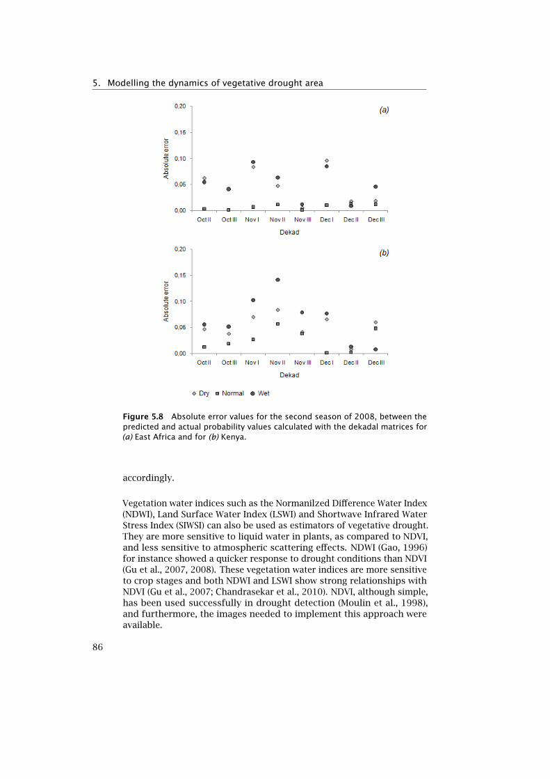
5. Modelling the dynamics of vegetative drought area
Figure 5.8 Absolute error values for the second season of 2008, between thepredicted and actual probability values calculated with the dekadal matrices for(a) East Africa and for (b) Kenya.
accordingly.
Vegetation water indices such as the Normanilzed Difference Water Index(NDWI), Land Surface Water Index (LSWI) and Shortwave Infrared WaterStress Index (SIWSI) can also be used as estimators of vegetative drought.They are more sensitive to liquid water in plants, as compared to NDVI,and less sensitive to atmospheric scattering effects. NDWI (Gao, 1996)for instance showed a quicker response to drought conditions than NDVI(Gu et al., 2007, 2008). These vegetation water indices are more sensitiveto crop stages and both NDWI and LSWI show strong relationships withNDVI (Gu et al., 2007; Chandrasekar et al., 2010). NDVI, although simple,has been used successfully in drought detection (Moulin et al., 1998),and furthermore, the images needed to implement this approach wereavailable.
86
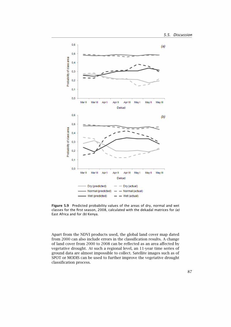
5.5. Discussion
Figure 5.9 Predicted probability values of the areas of dry, normal and wetclasses for the first season, 2008, calculated with the dekadal matrices for (a)East Africa and for (b) Kenya.
Apart from the NDVI products used, the global land cover map datedfrom 2000 can also include errors in the classification results. A changeof land cover from 2000 to 2008 can be reflected as an area affected byvegetative drought. At such a regional level, an 11-year time series ofground data are almost impossible to collect. Satellite images such as ofSPOT or MODIS can be used to further improve the vegetative droughtclassification process.
87
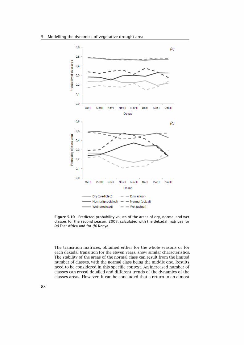
5. Modelling the dynamics of vegetative drought area
Figure 5.10 Predicted probability values of the areas of dry, normal and wetclasses for the second season, 2008, calculated with the dekadal matrices for(a) East Africa and for (b) Kenya.
The transition matrices, obtained either for the whole seasons or foreach dekadal transition for the eleven years, show similar characteristics.The stability of the areas of the normal class can result from the limitednumber of classes, with the normal class being the middle one. Resultsneed to be considered in this specific context. An increased number ofclasses can reveal detailed and different trends of the dynamics of theclasses areas. However, it can be concluded that a return to an almost
88
5.6. Conclusion
normal conditions, no matter the number classes being normal, is mostlikely to happen, as droughts are temporary phenomena.
In Kenya, the higher probability to stay wet can be explained by the factthat Kenya has a different rainfall regime in its north. The local specificityof the vegetation type for instance, not having a significant impact onthe overall East Africa region, can also cause the wet class to remain wetin this study. Although rainfall occurs seasonally throughout most ofKenya, the highlands of western Kenya have a single rainy season, lastingfrom March to September. Hence the importance of selecting seasonshomogenous to the study area, as the parameters a, b and m are derivedfrom the selected seasons.
The use of the dekadal transition matrices rather than the ones estimatedfor the entire seasons better captured the trend of the probabilities ofclass areas. In effect, as for instance rainfall amount varies during a sea-son, the changes of vegetative drought vary throughout the season; usinga seasonal matrix will smooth this effect. The growth cycle of plants canalso play a role. Dekadal matrices are then more accurate to capture thetrend of the dynamics. Results of tests of Markov properties show thatthe transition probabilities in East Africa are not homogeneous, whilefor Kenya they are. In both cases though, the use of dekadal transitionmatrices performed better for prediction, than the seasonal matrices.As the initial distribution vector is reset for every prediction, and thatthe dekadal transition matrices give more details of the changes, thestationarity of the seasonal matrices is not an issue.
The values of the areas predicted differ from the actual values for dif-ferent potential reasons: the change in the land cover since 2000 caninfluence the prediction results as well, and the prediction process mightinvolve more parameters than the transition matrices multiplied by theinitial probability distribution vectors.
With proper consideration of the specificity of a region, the proposedmethods can be used to model the dynamics of vegetative drought inother regions of the World.
5.6 Conclusion
Markov chains offer possibilities to understand and model the dynamicsof vegetative drought classes using the areas. With transition matricescalculated based on 3 classes, East Africa show higher probability valuesto remain or return to normal classes (0.5). Kenya show a similar pattern,with however a slightly higher value to remain wet. The probabilitytransition matrices are multiplied by current probabilities of the size ofarea of the classes and results show that the area of the normal classis predicted with more accuracy (λ = 0.01) than the areas of the other
89
5. Modelling the dynamics of vegetative drought area
classes. The use of the dekadal probability transition matrices reducedthe errors between the predicted and the actual values. These resultscan serve to first understand the dynamics of vegetative drought on adekadal basis, and second to make an early estimate of damages. Whilelong-term prediction results can help drought policies to be implemented,short-term prediction results can help estimating the potential damagein case no drought policies are implemented. This can help in costestimation of losses of crops for instance. Further, these results can beintegrated with long-term drought forecast models’ outputs.
90
6Assessing the spatiotemporalmovement of vegetative drought
6.1 Introduction 936.2 Materials and Methods 946.3 Results 1006.4 Discussion 1066.4 Conclusion 106
This chapter is based on: C.M. Rulinda, A. Stein, U. Turdukulov. Visualiz-ing and quantifying the movement of vegetative drought using remotesensing data and GIS. Under review at the International Journal of Geograph-ical Information Science.
91
6. Assessing the spatiotemporal movement of vegetative drought
Abstract
Remote sensing-based drought monitoring methods provide fast anduseful information for a sustainable management strategy of droughtimpact over a region. Common pixel-based monitoring methods arelimited in the analysis of the dynamics of this impact at regional scale.For instance, these hardly allow to quantify the movement of drought inspace and time, and to compare drought with rainfall deficits withoutloosing the variability of these events within a region. This study pro-posed an object-based approach that allowed us to visualize and quantifythe spatiotemporal movement of drought impact on vegetation, calledvegetative drought, in a region. The GIS software Dynomap was used toextract and track objects. Measures of distance and angle were used fordetermining the speed and direction of vegetative drought and rainfalldeficit objects, calculated from the National Oceanic and AtmosphericAdministration noaa Normalized Difference Vegetation Index (NDVI) andfrom NOAA Rainfall Estimates (RFE) data. The methods were appliedto the two rainy seasons during the drought year 1999 in East Africa.Results showed that vegetative drought objects moved into the South-Western direction at an average angle of -138.5◦ during the first seasonand -144.5◦ during the second season. The speed of objects variedbetween 38 km dekad−1 and 185 km dekad−1 during the first season,and between 33 km dekad−1 and 144 km dekad−1 during the secondseason, reflecting the rate of spread between dekads. Vegetative droughtobjects close to rainfall deficit objects showed similar trajectories andsometimes regions overlapped. This indicated that the two events arerelated. We conclude that a spatio-temporal relationship existed betweenthe two types of events, and that could be quantified.
92
6.1. Introduction
6.1 Introduction
Drought is a temporary, common and recurrent feature of climate. Itoccurs in virtually all regions of the globe, but its characteristics mayvary throughout a region. In general, it originates from a deficiencyof precipitation over an extended period of time resulting in a watershortage for some sectors. Drought can have a substantial impact onthe ecosystem and agriculture of the affected region. Although no uni-versal definition exists, operational definitions are used to analyze thedrought duration, frequency and degree of severity (Whilite and Glantz,1987). These operational definitions are impact-based. The impact ofdrought on vegetation, referred to in this study as vegetative drought, canbe defined as the negative impact of drought on vegetation, and canbe characterized by how far from a determined normal condition, thevegetation condition has been negatively affected.
In vulnerable areas where vegetation health mainly depends upon rainfallsuch as in East Africa, vegetative drought can have a significant negativeimpact on socio-economic aspects. For instance, over the past years,various institutions reported failed, poor or delayed rainfall seasonsaffecting vegetation growth that resulted in famine, displacements, con-flicts and death of people and cattle. As drought develops and intensifies,the impact on vegetation spreads throughout a region. Analyzing thespatio-temporal movement of vegetative drought can improve our under-standing of the phenomena and help reducing the devastating effects.
In recent years, Geographic Information Science (GIS) and Remote Sens-ing (RS) have played a major role in studying drought, such as in studiesby Mokhtari et al. (2011); Murad and Islam Saiful (2011). Remote sensingvegetation indices such as the Normalized Difference Vegetation Index(NDVI) (Tucker, 1979) have been used to monitor the response of ve-getation to climatic fluctuations in East Africa (Nicholson et al., 1990;Davenport and Nickolson, 1993; Eklundh, 1996, 1998), as an indication ofvegetative drought. Furthermore, issues of geospatial data quality havebeen addressed and the vague characterisation of vegetative droughtwas modeled (Rulinda et al., 2012) using a fuzzy classification approach(Wang, 1990). These advancements allowed us to quantify the dynamicsof vegetative drought with measures of certainties, however withoutproviding with an understanding of the spatio-temporal movement ofvegetative drought at a regional scale. For that purpose, an object-basedapproach was proposed. Advancements have also been made during thepast years in the development of object-based image analysis (de Jonget al., 2001; Stein et al., 2009; Blaschke et al., 2008; Blaschke, 2010;Blaschke et al., 2011; Mokhtari et al., 2011). The main difference betweenpixel-based and object-based image analyses is that the object-basedoriented approaches provide output in the form of thematic maps thatare composed of geographical entities. The movement of these entities
93
6. Assessing the spatiotemporal movement of vegetative drought
can be quantified. Among others, Cheng et al. (1997) proposed methodsto identify fuzzy objects from Field observations. According to theirdefinitions, vegetative drought objects can be characterize in space asobjects with crisp boundaries and fuzzy interiors.
Visualization techniques to explore spatial data have been widely dis-cussed by Kraak and MacEachren (1999). As modeling uncertainty ingeospatial data was getting more attention, visualization techniques haveadapted and prototypes have been developed to present and exploreuncertainty in remote sensing data (Lucieer and Kraak (2004)). The propo-type Dynomap developed by Turdukulov et al. (2005); Turdukolov (2007)in envi/idlo is a tool that allows one to visualize the evolution of entitiesin remote sensing images. It can handle entities with crisp boundariesand fuzzy interiors. In this study, we proposed a method to visualizeand quantify the spatiotemporal movement of vegetative drought overEast Africa using satellite data for characterization of entities of interest,and using Dynomap for extraction and tracking of these entities.
6.2 Materials and Methods
6.2.1 Study area
The study area, as shown in Figure 1.6, covers a subset of East Africathat includes five countries namely Burundi, Kenya, Uganda, Tanzaniaand Rwanda. The region, also referred to as the East Africa Community(EAC), is situated between the latitude 4◦ N and 2◦ S, and longitude 28◦ Eand 42◦ E. It covers a surface of 1.82 million km 2, with a population ofmore than 133.5 million. The climate in East Africa is predominantlysemi-arid. The growing season in most of East Africa follows the tworainy season pattern: an abundant rainy season from March to May anda second one less abundant, from October to December.
East Africa is a drought prone region. It has been affected by droughtsince the 1980s. The United Nations Children’s Fund (UNICEF) reporteda serious drought that has been developing in Eastern Africa since early1999 (UNICEF, 2000). The Food and Agriculture Organization (FAO) alsoreported serious crop failures in several regions of Tanzania, in Novem-ber 1999 (FAO/GIEWS, 1999). In Kenya, significant harvest shortfallswere forecast during the same period in several parts due to drought,and worsening nutritional conditions were reported in pastoral and agro-pastoral areas (FAO/GIEWS, 1999). At the same period, in Burundi andRwanda, inadequate rainfall affected the recently harvested crops. In thischapter, the drought year of 1999 is analyzed for different rainy seasons.
94
6.2. Materials and Methods
6.2.2 Data and processing
During the past two decades, vegetation indices data such as the NDVI(Tucker, 1979) have been used in studies to monitor the response ofvegetation to climatic fluctuations in East Africa (Nicholson et al., 1990),(Davenport and Nickolson, 1993) (Eklundh, 1996), (Eklundh, 1998). Thesestudies concluded that temporal variations of NDVI are closely linked toprecipitation with the best correlation between NDVI and the concurrentmonth plus two previous months (Nicholson et al., 1990), (Davenportand Nickolson, 1993).
On the basis of the primary understanding of vegetative drought as aperiod during which vegetation health is below normal due to a waterdeficit (especially rainfall), two datasets were considered for this study:The NDVI and RFE datasets. NDVI and RFE images from the NationalOceanic and Atmospheric Administration (NOAA) were acquired andused with the characteristics show in Table A.1. Vegetative drought (vd)and cumulative RFE deficit (rd) values are calculated from these datasetsand used to analyze the spatio-temporal dynamics of vegetative drought.The process of obtaining vd and rd images is explained in sections below.
A. Vegetative drought images
NOAA-AVHRR derived 10-days (dekad) NDVI products are processed bythe Global Inventory Monitoring and Modeling Systems (GIMMS) group(Tucker et al., 2005), (Pinzón et al., 2005) at the US National AeronauticSpace Agency (NASA/GSFC). The GLC2000 (EC-JRC-GEMU, 2000) LandCover map is used to mask out non-vegetated area and forests. Threeclasses according to the GLC2000 Africa-v5-legend are considered: (7)Mosaic forest/croplands, (18) Croplands ( > 50 %) and (19) Croplandswith open woody vegetation.Data from March to May 1999 and from October 1999 to January 2000are used. The dekadal long-term mean NDVI are calculated from the year1982 through the year 2008. AVHRR NDVI values in the range [0, 1] arelinearly stretched to [0, 250] whereas missing and erroneous values areassigned to the value 253. The pixel resolution of the images is 8 km.From the original images, subsets covering the region of interest (Figure1.6) are extracted.
As low NDVI values do not reflect vegetative drought, but a low density ofvegetation, vegetative drought can be characterized using the departureof the current NDVI values from the concurrent long-term mean NDVIvalues. Values of this departure, referred to as differenceNDVI values,denoted x, are calculated as the difference between current NDVI andlong-term mean NDVI values (Anyamba and Tucker, 2011), (Thenkabailet al., 2004), (Murad and Islam Saiful, 2011). Positive difference valuesindicate above normal conditions. Missing, erroneous or water values areall assigned to 250. Negative difference values, denoted by x, indicate
95
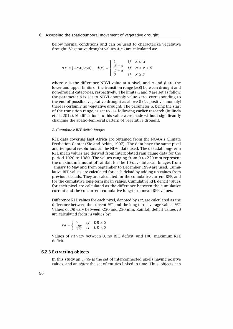
6. Assessing the spatiotemporal movement of vegetative drought
below normal conditions and can be used to characterize vegetativedrought. Vegetative drought values d(x) are calculated as:
∀x ∈ [−250,250], d(x) =
1 if x ≤ αβ− xβ− a if α < x < β
0 if x ≥ β
where x is the difference NDVI value at a pixel, and α and β are thelower and upper limits of the transition range ]α,β[ between drought andnon-drought categories, respectively. The limits α and β are set as follow:the parameter β is set to NDVI anomaly value zero, corresponding tothe end of possible vegetative drought as above 0 (i.e. positive anomaly)there is certainly no vegetative drought. The parameter α, being the startof the transition range, is set to -14 following earlier research (Rulindaet al., 2012). Modifications to this value were made without significantlychanging the spatio-temporal pattern of vegetative drought.
B. Cumulative RFE deficit images
RFE data covering East Africa are obtained from the NOAA’s ClimatePrediction Center (Xie and Arkin, 1997). The data have the same pixeland temporal resolutions as the NDVI data used. The dekadal long-termRFE mean values are derived from interpolated rain gauge data for theperiod 1920 to 1980. The values ranging from 0 to 250 mm representthe maximum amount of rainfall for the 10-days interval. Images fromJanuary to May and from September to December 1999 are used. Cumu-lative RFE values are calculated for each dekad by adding up values fromprevious dekads. They are calculated for the cumulative current RFE, andfor the cumulative long-term mean values. Cumulative RFE deficit values,for each pixel are calculated as the difference between the cumulativecurrent and the concurrent cumulative long-term mean RFE values.
Difference RFE values for each pixel, denoted by DR, are calculated as thedifference between the current RFE and the long-term average values RFE.Values of DR vary between -250 and 250 mm. Rainfall deficit values rdare calculated from ra values by:
rd ={
0 if DR ≥ 0−DR2.5 if DR < 0
Values of rd vary between 0, no RFE deficit, and 100, maximum RFEdeficit.
6.2.3 Extracting objects
In this study an entity is the set of interconnected pixels having positvevalues, and an object the set of entities linked in time. Thus, objects can
96
6.2. Materials and Methods
be quantified and they can be compared in space and time. The object-based approach is used here to analyze the movement of vegetativedrought and rainfall deficit objects in space and time. To do so, Iused the tracking-visualization tool, Dynomap, developed by Turdukulovet al. (2005, 2007) in ENVI/IDL. The tool allows to extract entities withcrisp boundaries and fuzzy interiors, hence accounting for the spatialvariability of values within the entities. As the interest is in extractinggroups of pixels with positive values (> 0) from background values (0),entities with crisp boundaries are the chosen concept. These entities areextracted as objects with the following attributes:
• Entity ID that uniquely identifies an object at time t.
• Time t.
• The total-area, or the spatial coverage of the entity, calculatedas in Equation (6.1) and the mean-area calculated as in Equation(6.2) below. To calculate total-area and mean-area, the study usedmeasures adapted from the ones proposed by Dilo (2006); Diloet al. (2007a) for continuous space. In the following equations, K isused to denote the entity, ρ(p) to indicate either d(x)(p) and rd(p)values for pixel p of the entity. The total-area of K is calculatedby:
total-area(K) =∑p∈K|p| (6.1)
where |p| is the pixel size.
The mean-area of entity (K) is calculated as in equation (6.2), by:
mean-area(K) =∑p∈K
ρ(p) · |p| (6.2)
where ρ(p) indicates either d(x)(p) and rd(p) values for pixel p.The mean-area of entity K is thus equal to the pixel size multipliedby the sum of ρ(p) for all p pixels in K.
• The centroids, or center of mass of entities are extracted to trackobjects. The coordinates of the centroids, Cx and Cy , are calculatedfor each entity K as:
Cx(K) =∑p∈K |p|x · ρ(p)∑
p∈K ρ(p)(6.3)
Cy(K) =∑p∈K |p|y · ρ(p)∑
p∈K ρ(p)(6.4)
where |p|x and |p|y indicate the size of the pixel along the x and ydirections respectively.
97
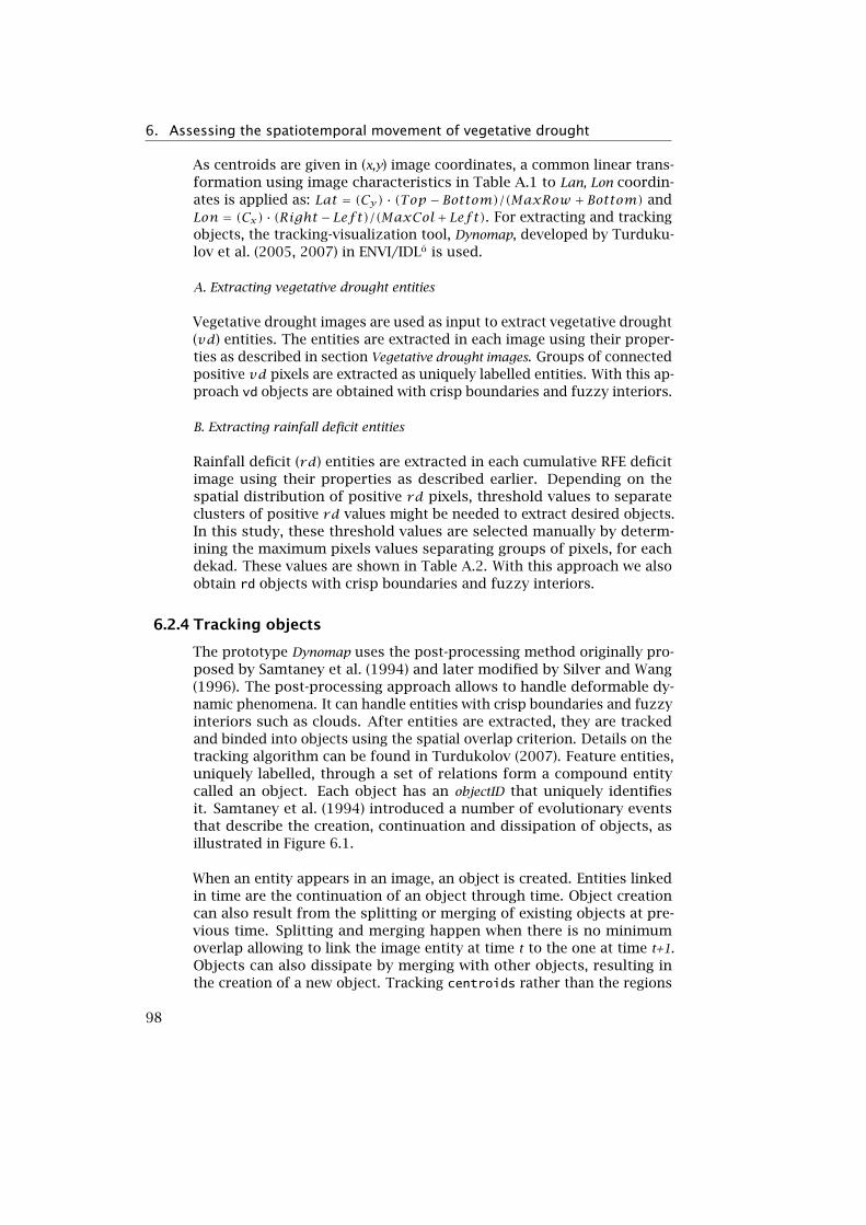
6. Assessing the spatiotemporal movement of vegetative drought
As centroids are given in (x,y) image coordinates, a common linear trans-formation using image characteristics in Table A.1 to Lan, Lon coordin-ates is applied as: Lat = (Cy) · (Top − Bottom)/(MaxRow + Bottom) andLon = (Cx) · (Right−Left)/(MaxCol+Left). For extracting and trackingobjects, the tracking-visualization tool, Dynomap, developed by Turduku-lov et al. (2005, 2007) in ENVI/IDLo is used.
A. Extracting vegetative drought entities
Vegetative drought images are used as input to extract vegetative drought(vd) entities. The entities are extracted in each image using their proper-ties as described in section Vegetative drought images. Groups of connectedpositive vd pixels are extracted as uniquely labelled entities. With this ap-proach vd objects are obtained with crisp boundaries and fuzzy interiors.
B. Extracting rainfall deficit entities
Rainfall deficit (rd) entities are extracted in each cumulative RFE deficitimage using their properties as described earlier. Depending on thespatial distribution of positive rd pixels, threshold values to separateclusters of positive rd values might be needed to extract desired objects.In this study, these threshold values are selected manually by determ-ining the maximum pixels values separating groups of pixels, for eachdekad. These values are shown in Table A.2. With this approach we alsoobtain rd objects with crisp boundaries and fuzzy interiors.
6.2.4 Tracking objects
The prototype Dynomap uses the post-processing method originally pro-posed by Samtaney et al. (1994) and later modified by Silver and Wang(1996). The post-processing approach allows to handle deformable dy-namic phenomena. It can handle entities with crisp boundaries and fuzzyinteriors such as clouds. After entities are extracted, they are trackedand binded into objects using the spatial overlap criterion. Details on thetracking algorithm can be found in Turdukolov (2007). Feature entities,uniquely labelled, through a set of relations form a compound entitycalled an object. Each object has an objectID that uniquely identifiesit. Samtaney et al. (1994) introduced a number of evolutionary eventsthat describe the creation, continuation and dissipation of objects, asillustrated in Figure 6.1.
When an entity appears in an image, an object is created. Entities linkedin time are the continuation of an object through time. Object creationcan also result from the splitting or merging of existing objects at pre-vious time. Splitting and merging happen when there is no minimumoverlap allowing to link the image entity at time t to the one at time t+1.Objects can also dissipate by merging with other objects, resulting inthe creation of a new object. Tracking centroids rather than the regions
98
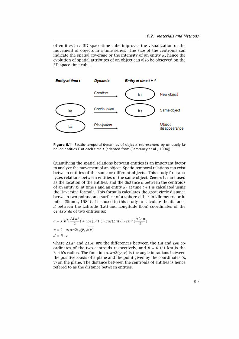
6.2. Materials and Methods
of entities in a 3D space-time cube improves the visualization of themovement of objects in a time series. The size of the centroids canindicate the spatial coverage or the intensity of an entity K, hence theevolution of spatial attributes of an object can also be observed on the3D space-time cube.
Figure 6.1 Spatio-temporal dynamics of objects represented by uniquely la-belled entities E at each time t (adapted from (Samtaney et al., 1994)).
Quantifying the spatial relations between entities is an important factorto analyze the movement of an object. Spatio-temporal relations can existbetween entities of the same or different objects. This study first ana-lyzes relations between entities of the same object. Centroids are usedas the location of the entities, and the distance d between the centroidsof an entity K1 at time t and an entity K2 at time t + 1 is calculated usingthe Haversine formula. This formula calculates the great-circle distancebetween two points on a surface of a sphere either in kilometers or inmiles (Sinnot, 1984) . It is used in this study to calculate the distanced between the Latitude (Lat) and Longitude (Lon) coordinates of thecentroids of two entities as:
a = sin2(∆Lat
2)+ cos(Lat1) · cos(Lat2) · sin2(
∆Lon2
)
c = 2 · atan2(√y,√(x)
d = R · c
where ∆Lat and ∆Lon are the differences between the Lat and Lon co-ordinates of the two centroids respectively, and R = 6.371 km is theEarth’s radius. The function atan2(y,x) is the angle in radians betweenthe positive x-axis of a plane and the point given by the coordinates (x,y) on the plane. The distance between the centroids of entities is hencerefered to as the distance between entities.
99
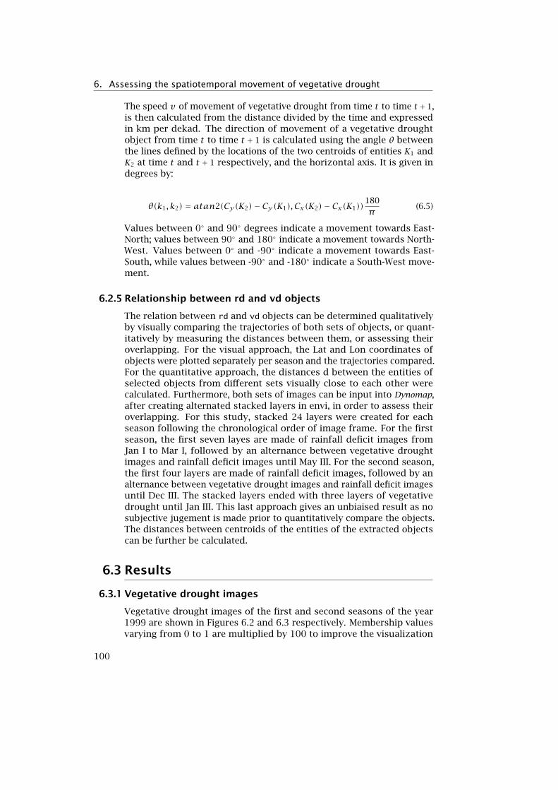
6. Assessing the spatiotemporal movement of vegetative drought
The speed v of movement of vegetative drought from time t to time t+1,is then calculated from the distance divided by the time and expressedin km per dekad. The direction of movement of a vegetative droughtobject from time t to time t + 1 is calculated using the angle θ betweenthe lines defined by the locations of the two centroids of entities K1 andK2 at time t and t + 1 respectively, and the horizontal axis. It is given indegrees by:
θ(k1, k2) = atan2(Cy(K2)− Cy(K1), Cx(K2)− Cx(K1))180π
(6.5)
Values between 0◦ and 90◦ degrees indicate a movement towards East-North; values between 90◦ and 180◦ indicate a movement towards North-West. Values between 0◦ and -90◦ indicate a movement towards East-South, while values between -90◦ and -180◦ indicate a South-West move-ment.
6.2.5 Relationship between rd and vd objects
The relation between rd and vd objects can be determined qualitativelyby visually comparing the trajectories of both sets of objects, or quant-itatively by measuring the distances between them, or assessing theiroverlapping. For the visual approach, the Lat and Lon coordinates ofobjects were plotted separately per season and the trajectories compared.For the quantitative approach, the distances d between the entities ofselected objects from different sets visually close to each other werecalculated. Furthermore, both sets of images can be input into Dynomap,after creating alternated stacked layers in envi, in order to assess theiroverlapping. For this study, stacked 24 layers were created for eachseason following the chronological order of image frame. For the firstseason, the first seven layes are made of rainfall deficit images fromJan I to Mar I, followed by an alternance between vegetative droughtimages and rainfall deficit images until May III. For the second season,the first four layers are made of rainfall deficit images, followed by analternance between vegetative drought images and rainfall deficit imagesuntil Dec III. The stacked layers ended with three layers of vegetativedrought until Jan III. This last approach gives an unbiaised result as nosubjective jugement is made prior to quantitatively compare the objects.The distances between centroids of the entities of the extracted objectscan be further be calculated.
6.3 Results
6.3.1 Vegetative drought images
Vegetative drought images of the first and second seasons of the year1999 are shown in Figures 6.2 and 6.3 respectively. Membership valuesvarying from 0 to 1 are multiplied by 100 to improve the visualization
100
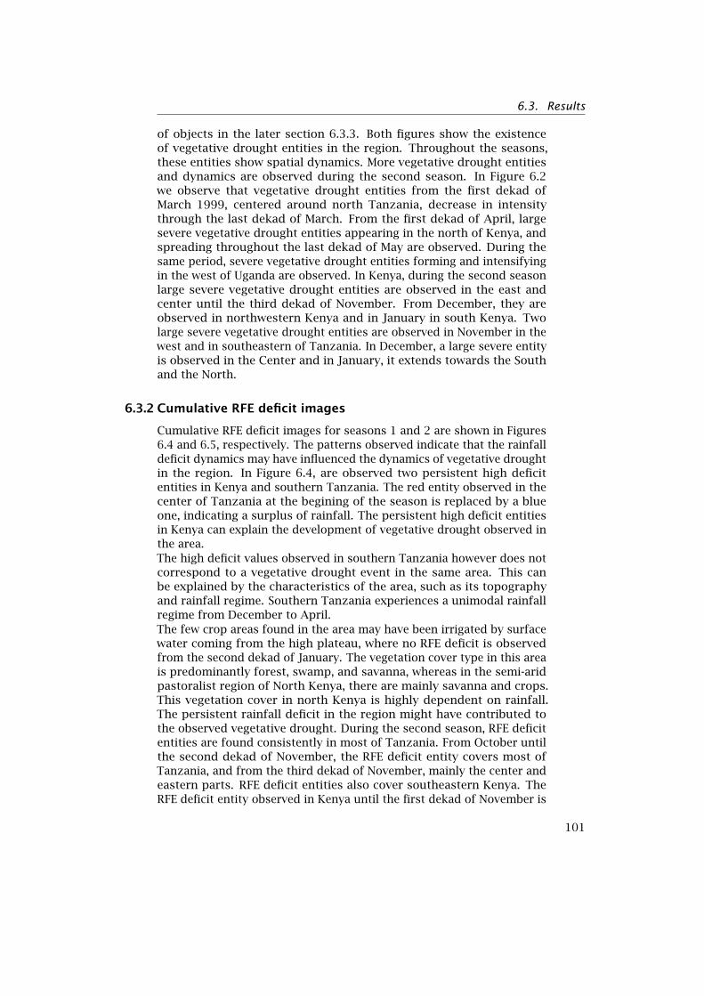
6.3. Results
of objects in the later section 6.3.3. Both figures show the existenceof vegetative drought entities in the region. Throughout the seasons,these entities show spatial dynamics. More vegetative drought entitiesand dynamics are observed during the second season. In Figure 6.2we observe that vegetative drought entities from the first dekad ofMarch 1999, centered around north Tanzania, decrease in intensitythrough the last dekad of March. From the first dekad of April, largesevere vegetative drought entities appearing in the north of Kenya, andspreading throughout the last dekad of May are observed. During thesame period, severe vegetative drought entities forming and intensifyingin the west of Uganda are observed. In Kenya, during the second seasonlarge severe vegetative drought entities are observed in the east andcenter until the third dekad of November. From December, they areobserved in northwestern Kenya and in January in south Kenya. Twolarge severe vegetative drought entities are observed in November in thewest and in southeastern of Tanzania. In December, a large severe entityis observed in the Center and in January, it extends towards the Southand the North.
6.3.2 Cumulative RFE deficit images
Cumulative RFE deficit images for seasons 1 and 2 are shown in Figures6.4 and 6.5, respectively. The patterns observed indicate that the rainfalldeficit dynamics may have influenced the dynamics of vegetative droughtin the region. In Figure 6.4, are observed two persistent high deficitentities in Kenya and southern Tanzania. The red entity observed in thecenter of Tanzania at the begining of the season is replaced by a blueone, indicating a surplus of rainfall. The persistent high deficit entitiesin Kenya can explain the development of vegetative drought observed inthe area.The high deficit values observed in southern Tanzania however does notcorrespond to a vegetative drought event in the same area. This canbe explained by the characteristics of the area, such as its topographyand rainfall regime. Southern Tanzania experiences a unimodal rainfallregime from December to April.The few crop areas found in the area may have been irrigated by surfacewater coming from the high plateau, where no RFE deficit is observedfrom the second dekad of January. The vegetation cover type in this areais predominantly forest, swamp, and savanna, whereas in the semi-aridpastoralist region of North Kenya, there are mainly savanna and crops.This vegetation cover in north Kenya is highly dependent on rainfall.The persistent rainfall deficit in the region might have contributed tothe observed vegetative drought. During the second season, RFE deficitentities are found consistently in most of Tanzania. From October untilthe second dekad of November, the RFE deficit entity covers most ofTanzania, and from the third dekad of November, mainly the center andeastern parts. RFE deficit entities also cover southeastern Kenya. TheRFE deficit entity observed in Kenya until the first dekad of November is
101
6. Assessing the spatiotemporal movement of vegetative drought
Figure 6.2 Vegetative drought images of East Africa from the first dekad ofMarch to the third dekad of May 1999. Vegetative drought membership valuesvary from 0 (no drought) and 100 (severe drought).
replaced by no RFE deficit entities from the second dekad of November,except for the northern part bordering Uganda. Vegetative droughtentities observed in those regions may have resulted from the high RFEdeficit in northen Kenya and in Tanzania.
6.3.3 Vegetative drought objects
Vegetative drought objects, denoted vd, are extracted in a similar wayfor both seasons. The locations of the centroids of extracted objects areshown in Figure 6.6 for both seasons. For the first season, 128 objects
102
6.3. Results
are extracted, while for the second season, 215 objects are extracted.Two large objects that persist throughout most of the seasons are ob-served with dynamics of the centroids corresponding to the patternsobserved in vegetative drought images. Table A.3 gives the locations ofthe centroids of these objects at each dekad.
In Figures 6.6 (a) and (b), the centroids of the vd object vd1 (in blue)are observed in March 1999, around the North of Tanzania. From Aprilonwards the object shifts towards south and its size decreases beforedissipating into the second dekad of May. A smaller object vd77 (inpurple) is observed from April 1999 through the end of the seasonin north Kenya, shifting slightly towards the center. In Figure 6.6 (c)and (d) we observe a vegetative drought object vd24 (in green) startingin eastern Kenya and shifting south towards the center of Tanzania.Another vegetative drought object vd115 (in dark blue) smaller than thefirst one, is also observed around northeastern Kenya from the end ofOctober to the end of November. The change of the size of centroidsindicates the change in the spatial coverage, i.e. shrinkage or expansionof the objects. The shifting of the centroids indicates either that thecenter of intensity of the object has moved to another area of the entity,the entities have shifted, or a combination of the above. In the nextsection these dynamics are analyzed.
6.3.4 Dynamics of vd objects
Distances between the centroids of each entity of the same object arecalculated and shown in Table A.4. On average, objects of longer dura-tions move faster than objects of shorter durations. When consideringsmaller time interval of objects, the speed can vary significantly. Objectvd1, with an average speed of 185 km dekad−1 moves faster than vd77with an average speed of 38 km dekad−1; and vd24, with an average speedof 144 km dekad−1 moves faster than vd115, with an average speed ofonly 33 km dekad−1.When considering vd24 at the time interval between the third dekadof October and the first dekad of November, the speed of movementequals 674 km dekad−1, whereas from the first to the second dekad ofNovember it is 33 km dekad−1. From these results it can be concludedthat the long distances or high speed values of a drought object at atime interval reflect considerable changes of the variability of vegetativedrought intensity in the region.
The directions of the movement of vegetative drought are calculatedas angles on a dekadal basis, and shown in Table A.4. The angles θcalculated between the lines formed by the coordinates of the centroidsof the first and last entities of each vd objects are shown in Table 6.1.These angles indicate that vegetative drought moved South-West fromits origin, when considering these four objects.
103
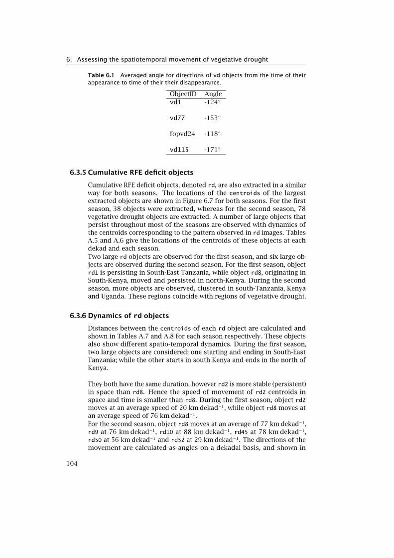
6. Assessing the spatiotemporal movement of vegetative drought
Table 6.1 Averaged angle for directions of vd objects from the time of theirappearance to time of their their disappearance.
ObjectID Anglevd1 -124◦
vd77 -153◦
fopvd24 -118◦
vd115 -171◦
6.3.5 Cumulative RFE deficit objects
Cumulative RFE deficit objects, denoted rd, are also extracted in a similarway for both seasons. The locations of the centroids of the largestextracted objects are shown in Figure 6.7 for both seasons. For the firstseason, 38 objects were extracted, whereas for the second season, 78vegetative drought objects are extracted. A number of large objects thatpersist throughout most of the seasons are observed with dynamics ofthe centroids corresponding to the pattern observed in rd images. TablesA.5 and A.6 give the locations of the centroids of these objects at eachdekad and each season.Two large rd objects are observed for the first season, and six large ob-jects are observed during the second season. For the first season, objectrd1 is persisting in South-East Tanzania, while object rd8, originating inSouth-Kenya, moved and persisted in north-Kenya. During the secondseason, more objects are observed, clustered in south-Tanzania, Kenyaand Uganda. These regions coincide with regions of vegetative drought.
6.3.6 Dynamics of rd objects
Distances between the centroids of each rd object are calculated andshown in Tables A.7 and A.8 for each season respectively. These objectsalso show different spatio-temporal dynamics. During the first season,two large objects are considered; one starting and ending in South-EastTanzania; while the other starts in south Kenya and ends in the north ofKenya.
They both have the same duration, however rd2 is more stable (persistent)in space than rd8. Hence the speed of movement of rd2 centroids inspace and time is smaller than rd8. During the first season, object rd2moves at an average speed of 20 km dekad−1, while object rd8 moves atan average speed of 76 km dekad−1.For the second season, object rd8 moves at an average of 77 km dekad−1,rd9 at 76 km dekad−1, rd10 at 88 km dekad−1, rd45 at 78 km dekad−1,rd50 at 56 km dekad−1 and rd52 at 29 km dekad−1. The directions of themovement are calculated as angles on a dekadal basis, and shown in
104
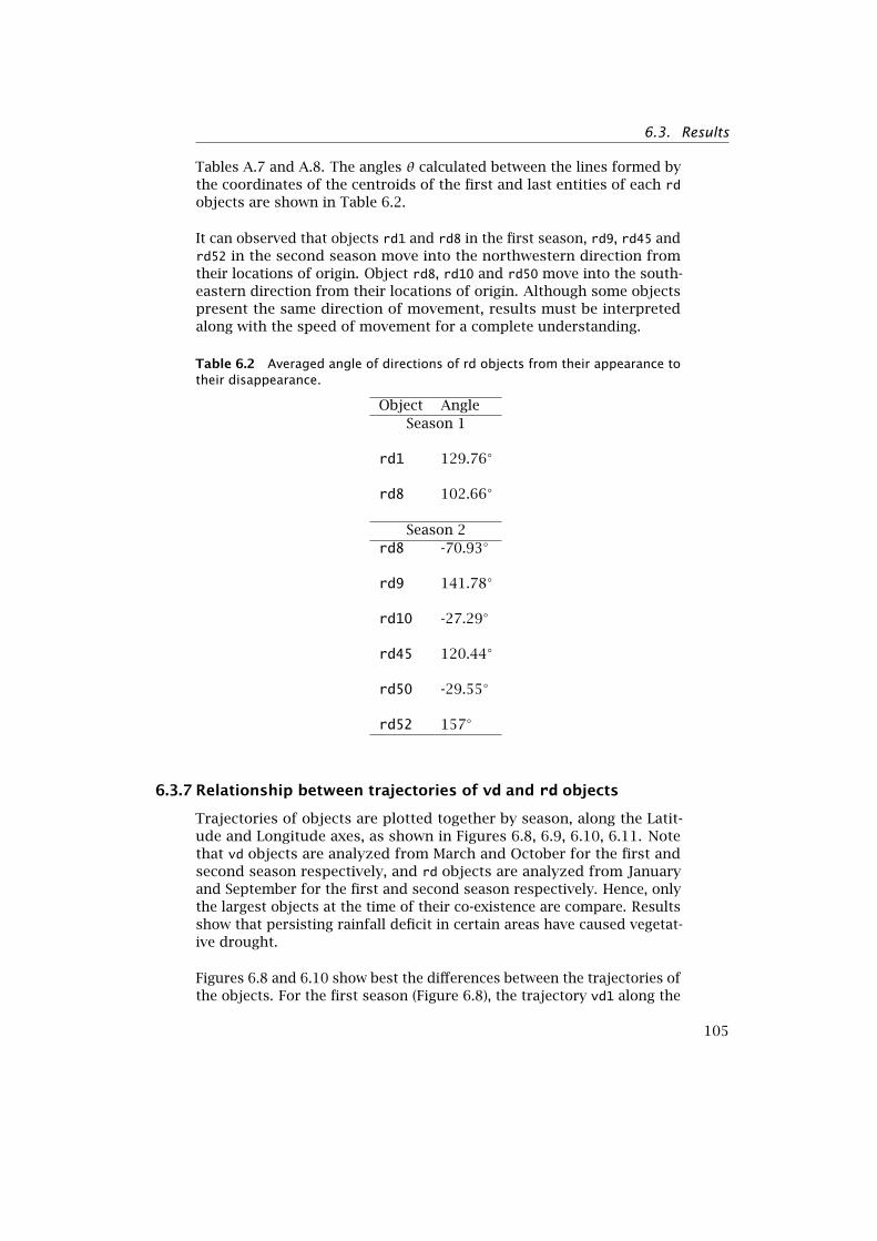
6.3. Results
Tables A.7 and A.8. The angles θ calculated between the lines formed bythe coordinates of the centroids of the first and last entities of each rdobjects are shown in Table 6.2.
It can observed that objects rd1 and rd8 in the first season, rd9, rd45 andrd52 in the second season move into the northwestern direction fromtheir locations of origin. Object rd8, rd10 and rd50 move into the south-eastern direction from their locations of origin. Although some objectspresent the same direction of movement, results must be interpretedalong with the speed of movement for a complete understanding.
Table 6.2 Averaged angle of directions of rd objects from their appearance totheir disappearance.
Object AngleSeason 1
rd1 129.76◦
rd8 102.66◦
Season 2rd8 -70.93◦
rd9 141.78◦
rd10 -27.29◦
rd45 120.44◦
rd50 -29.55◦
rd52 157◦
6.3.7 Relationship between trajectories of vd and rd objects
Trajectories of objects are plotted together by season, along the Latit-ude and Longitude axes, as shown in Figures 6.8, 6.9, 6.10, 6.11. Notethat vd objects are analyzed from March and October for the first andsecond season respectively, and rd objects are analyzed from Januaryand September for the first and second season respectively. Hence, onlythe largest objects at the time of their co-existence are compare. Resultsshow that persisting rainfall deficit in certain areas have caused vegetat-ive drought.
Figures 6.8 and 6.10 show best the differences between the trajectories ofthe objects. For the first season (Figure 6.8), the trajectory vd1 along the
105
6. Assessing the spatiotemporal movement of vegetative drought
Latitude direction is close to rd8, while vd77 is closer to rd8 at the firstdekad of March, and moves towards rd2. The object vd1 can have beeninfluenced first by the rd8, and later on by the object rd2. The distancesd between the co-existing entities of vd and rd objects are calculatedand shown in Table A.9. Results indicate that the distance between vd1and rd8 increased from 298 km to 1094 km through time, while it hasdecreased from 641 km to 512 km through time. The distance betweenvd77 and rd8 also decreased from 389 km to 248 km. This indicates thatpersisting rainfall deficits caused vegetative drought within a maximumdistance of 512 km.
During the second season (Figure 6.11), we observe that the trajectoriesof rd10, rd45 and rd50 objects are closer to the trajectory of vd24, whilethe trajectories of rd9 and rd52 objects are closer to the trajectory ofvd115. Results, as indicated in Table A.9, show that distances betweenvd24 and rd10, vd24 and rd8, vd24 and rd45, vd115 and rd52, vd11 andrd9 decreased trough time, while the distance between vd24 and rd50increased. At the end of the observation period,i.e. co-existing period,persisting rainfall deficits on drought vulnerable areas caused vegetativedrought within a maximum distance of 617 km.
Figure 6.12 show the relationship between the two events, obtainedby alternating rainfall deficit images and vegetative drought images inthe time series. The creation and persistence of objects show that vdand rd objects overlapped in the study area.
6.3.8 Sensitivity analysis of the tracking method
The tracking tool Dynomap allows to define the search radius for over-lapping of entities to form an object. In order to test the sensitivity ofthe vd tracking method, the search radius was set to 50 pixels. In otherwords, the tracking software will look for entities within a maximumradius of 50 pixels from time t to time t+1 to form an object path. Moreobjects are extracted for the first season (191) than without specifyingthe search radius, and the same amount of objects ( i.e. 215) are ex-tracted for the second season. The number of considerable objects ishowever unchanged. Vegetative drought (vd) objects extracted are vd1with unchanged properties, and vd78 with the properties of vd77 forthe first season; vd24 with unchanged properties, and vd137 with theproperties of vd115 for the second season. The locations of centroids ofthese objects are shown in Figure 6.13.
6.4 Discussion
Results indicate the existence of rainfall deficit and vegetative droughtevents in the East African region in 1999. It is expected that if thevegetation stress is caused by a rainfall deficits over the region, thelater covered persistently the areas before vegetative drought occurs. A
106
6.4. Discussion
qualitative analysis by visually comparing images to determine this rela-tion is limited as it can only offer a subjective interpretation, and it canbecome time consuming when many images are used; for instance, whenanalysing a multi-year drought. Existing alternative approaches, whileproviding with quantitative analysis methods, do not consider the spatialvariability of these events in a region of interest. Hence they are limitedin quantitative ways to analyze their spatio-temporal dynamics within aregion of interest. This study proposes an object-oriented analysis ap-proach to extract entities with crisp boundaries and fuzzy (multi-valued)interiors. This allows to capture the spatio-temporal variability of valueswithin each entity, as compared to feautures with crisp (single-valued)interiors. As only one category of an event, either vegetative droughtor cumulative rainfall deficit, is of interest, entities can be extracted onimages with crisp boundaries. The centroids are calculated and plottedto build the trajectories of each objects. Dynomap allows to select thesize of the centroids in regard to one attribute. This approach allowsin this study to visualize not only the movement of vd or rd objectsbut the evolution of the area of these objects as well. Results indicatethat rainfall deficits in East Africa may haved caused vegetative droughtin some areas, as demonstrated by other studies mentioned in section6.2.2. Visually comparing trajectories of both events show that there isa relation between them. Further studies to compare trajectories in aquantitative way can be developed, where the growing seasons are alsotaken into account.
Although the use of a membership function allows to account for thevague nature of vegetative drought, selecting threshold values to limit theclass from difference NDVI values remain a challenge. On the one hand,vegetative drought is characterized from NDVI anomaly values belownormal. In many areas, normal conditions generally mean conditionsthat do not deviate from long-term averages. However, these averagesthemselves can change over time. Results obtained should hence becarefully interpreted, related to the long-term mean period used. On theother hand, even while considering that the normal values are unchanged,selecting a value from which a vegetative drought starts and ends issubjective. In this method however, changing the parameters α and βdid not influence the conclusion about the spatio-temporal dynamics,only about the values of vegetative drought. Extracting and tracking rdobjects presented an additional challenge of segmentation, as the entitiesin the images are smoothed, hence spatially more connected than vdentities. This is caused by the modeled input data: although patches arevisually separable, they are spatially connected with positive rd valuespixels. A manual approach has been adopted here. The long-term meanvalues used to calculate RFE anomaly images are calculated for the yearsbefore 1999. Rainfall anomalies should then be considered relative to thelong-term period used. Results from this study are difficult to validateusing ground collected data due to the large geographical coverage ofvegetative drought and its characterization. Other remote sensing data
107
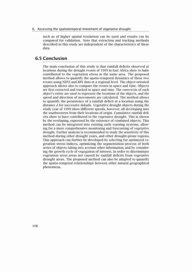
6. Assessing the spatiotemporal movement of vegetative drought
such as of higher spatial resolution can be used and results can becompared for validation. Note that extraction and tracking methodsdescribed in this study are independent of the characteristics of thesedata.
6.5 Conclusion
The main conclusion of this study is that rainfall deficits observed atlocations during the drought events of 1999 in East Africa show to habecontributed to the vegetation stress in the same area. The proposedmethod allows to quantify the spatio-temporal dynamics of these twoevents using NDVI and RFE data at a regional level. The object-orientedapproach allows also to compare the events in space and time. Objectsare first extracted and tracked in space and time. The centroids of eachobject’s entity are used to represent the locations of the objects, and thespeed and direction of movements are calculated. The method allowsto quantify the persistence of a rainfall deficit at a location using thedistance d for successive dekads. Vegetative drought objects during thestudy year of 1999 show different speeds, however, all developing intothe southwestern from their locations of origin. Cumulative rainfall defi-cits show to have contributed to the vegetative drought. This is shownby the overlaping, expressed by the existence of combined objects. Thismethod can be integrated into existing early warning systems, allow-ing for a more comprehensive monitoring and forecasting of vegetativedrought. Further analysis is recommended to study the sensitivity of thismethod during other drought years, and other drought-prone regions.This approach can further be developed by selecting for optimized ve-getation stress indices, optimizing the segmentation process of bothseries of objects taking into account other information, and by consider-ing the growth cycle of vegegation of interest, in order to discriminatevegetation sress areas not caused by rainfall deficits from vegetativedrought areas. The proposed method can also be adapted to quantifythe spatio-temporal relationships between other natural geographicalphenomena.
108
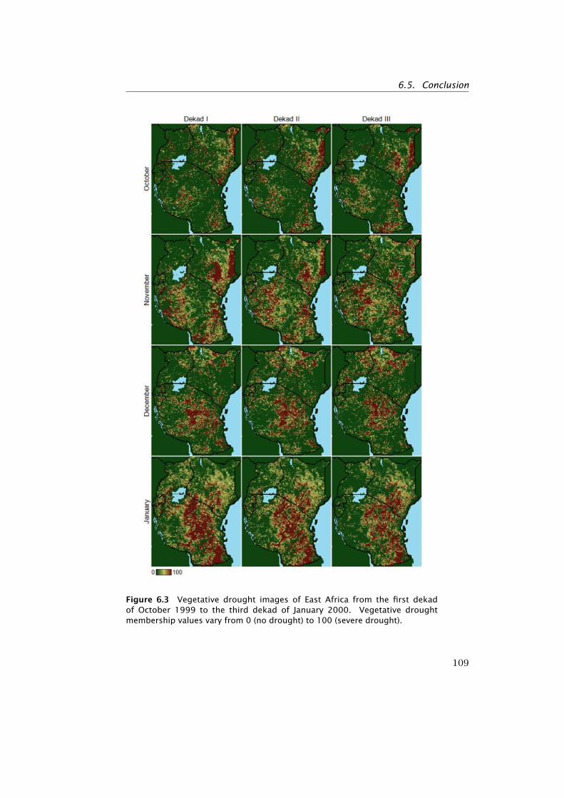
6.5. Conclusion
Figure 6.3 Vegetative drought images of East Africa from the first dekadof October 1999 to the third dekad of January 2000. Vegetative droughtmembership values vary from 0 (no drought) to 100 (severe drought).
109
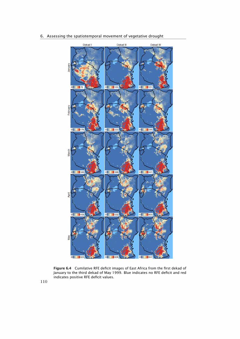
6. Assessing the spatiotemporal movement of vegetative drought
Figure 6.4 Cumilative RFE deficit images of East Africa from the first dekad ofJanuary to the third dekad of May 1999. Blue indicates no RFE deficit and redindicates positive RFE deficit values.
110
6.5. Conclusion
Figure 6.5 Cumilative RFE deficit images of East Africa from the first dekad ofSeptember to the third dekad of December 1999. Blue indicates no RFE deficitand red indicates positive RFE deficit values.
111
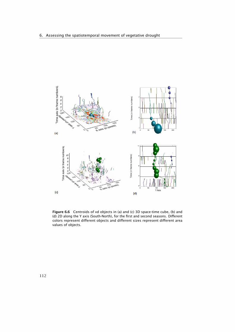
6. Assessing the spatiotemporal movement of vegetative drought
Figure 6.6 Centroids of vd objects in (a) and (c) 3D space-time cube, (b) and(d) 2D along the Y axis (South-North), for the first and second seasons. Differentcolors represent different objects and different sizes represent different areavalues of objects.
112
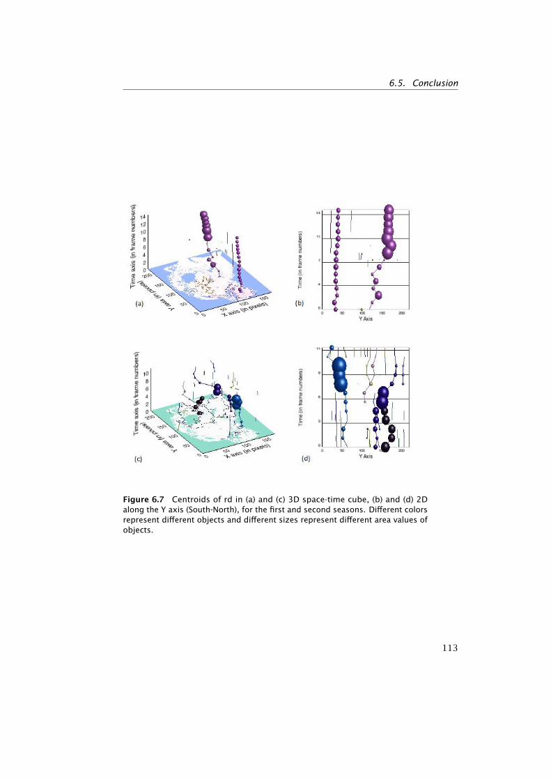
6.5. Conclusion
Figure 6.7 Centroids of rd in (a) and (c) 3D space-time cube, (b) and (d) 2Dalong the Y axis (South-North), for the first and second seasons. Different colorsrepresent different objects and different sizes represent different area values ofobjects.
113
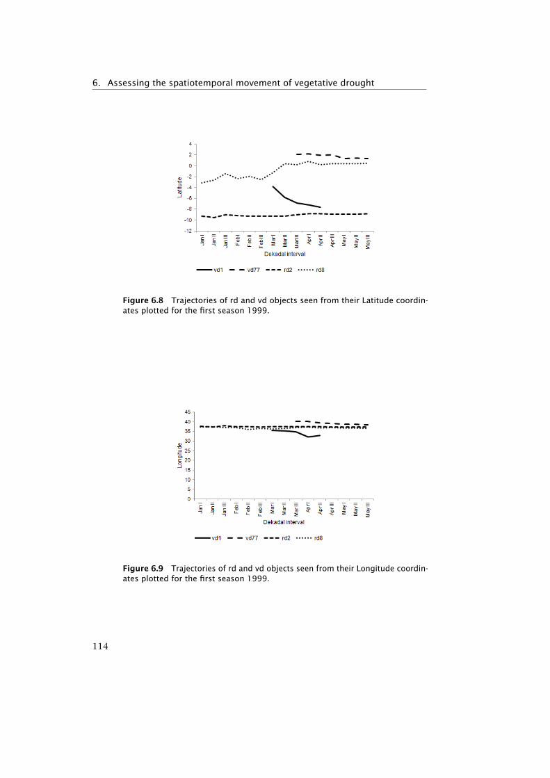
6. Assessing the spatiotemporal movement of vegetative drought
Figure 6.8 Trajectories of rd and vd objects seen from their Latitude coordin-ates plotted for the first season 1999.
Figure 6.9 Trajectories of rd and vd objects seen from their Longitude coordin-ates plotted for the first season 1999.
114
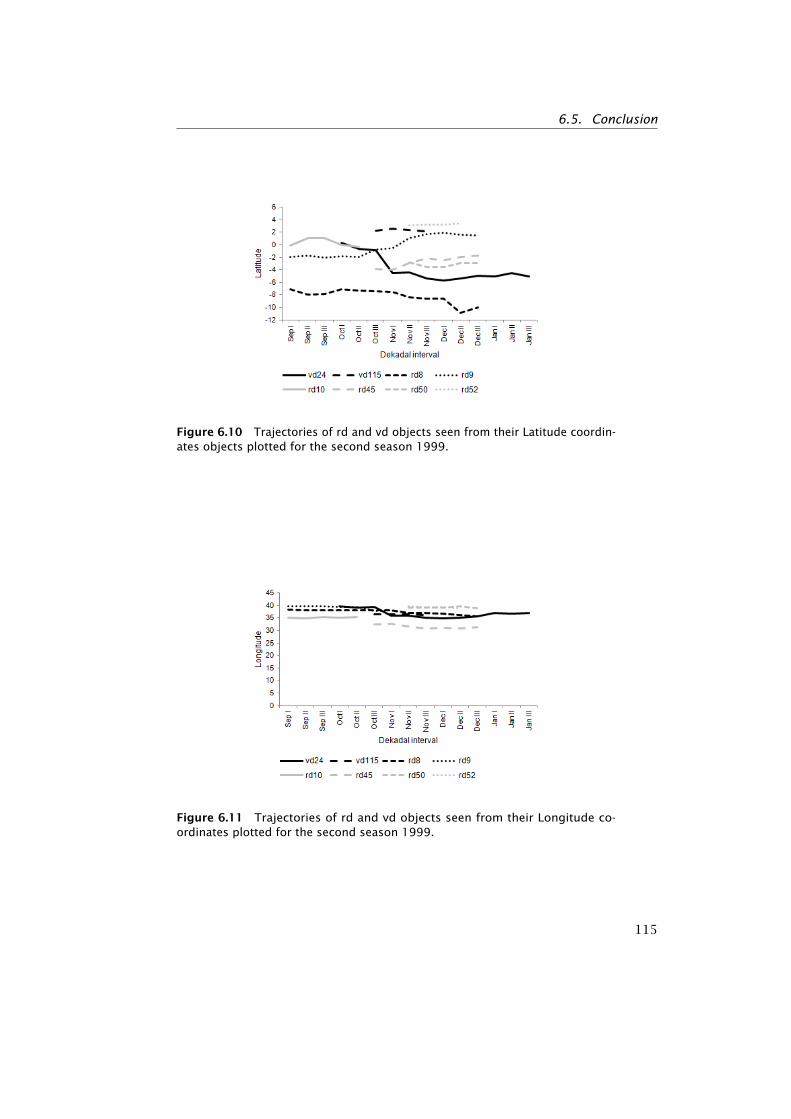
6.5. Conclusion
Figure 6.10 Trajectories of rd and vd objects seen from their Latitude coordin-ates objects plotted for the second season 1999.
Figure 6.11 Trajectories of rd and vd objects seen from their Longitude co-ordinates plotted for the second season 1999.
115
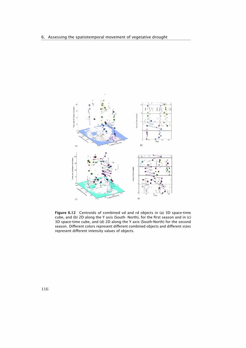
6. Assessing the spatiotemporal movement of vegetative drought
Figure 6.12 Centroids of combined vd and rd objects in (a) 3D space-timecube, and (b) 2D along the Y axis (South- North), for the first season and in (c)3D space-time cube, and (d) 2D along the Y axis (South-North) for the secondseason. Different colors represent different combined objects and different sizesrepresent different intensity values of objects.
116
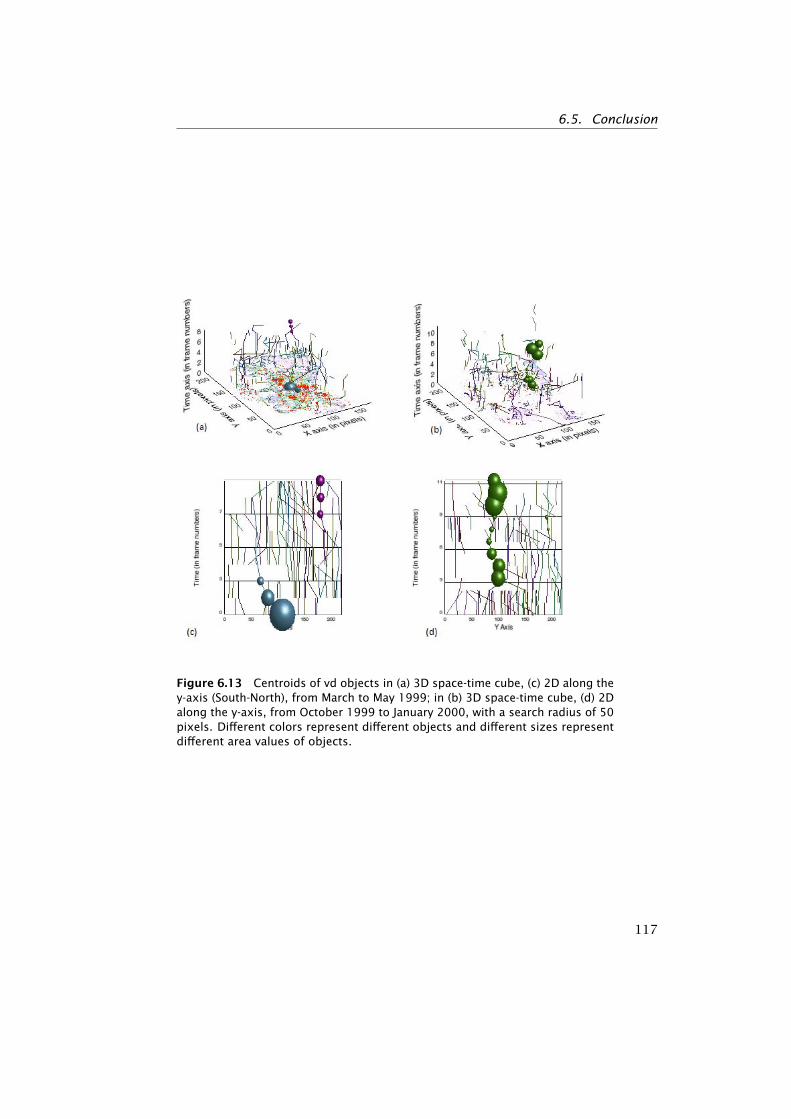
6.5. Conclusion
Figure 6.13 Centroids of vd objects in (a) 3D space-time cube, (c) 2D along they-axis (South-North), from March to May 1999; in (b) 3D space-time cube, (d) 2Dalong the y-axis, from October 1999 to January 2000, with a search radius of 50pixels. Different colors represent different objects and different sizes representdifferent area values of objects.
117

7Synthesis
7.1 Conclusions 1207.2 Reflection 124
7.2.1 Main contribution 1247.2.2 Opportunities for further research 125
119
7. Synthesis
7.1 Conclusions
In this section, the conclusions of research finding are presented assummary of results and discussions for specific research objectives asdescribed in section 1.2
7.1.1 Objective 1
The first objective was to improve the early detection of drought usingNDVI derived Meteosat SEVIRI data in eastern Africa. In doing so, usinga membership function to account for vagueness in the definition ofvegetative drought. In all the studies, vegetation stress was characterizedin space and time using the difference (DV) of current NDVI values fromtheir multi-year averaged values. These DV values were calculated bysubtracting the multi-year mean NDVI values from the current NDVIvalues. The observed vegetation stress is relative to the multi-year periodconsidered. A membership function was defined to model vegetativedrought from the DV values, while accounting for the vagueness resultingfrom its class definition. Results show that vegetative drought mem-bership values gradually increased in time at one selected area, namelyEmbu, in Kenya. This indicated a slow onset of vegetative drought at thelocation.
The major strengths and weaknesses of the proposed approach pertainto both the generation of DV time series and the selection of the member-ship function. Due to the short lifetime of operation of SEVIRI, the timeseries mean values were computed for a limited period of three years,introducing errors in DV values. The strength of the use of a membershipfunction compared to the traditional crisp function to model vegetativedrought, is that the gradual evolution of drought was taken into con-sideration. When vegetation stress is caused by another phenomenonthan drought, such as human or animal induced stress, the changes ofobserved NDVI vegetation values, the onset of vegetative drought, mightnot be gradual but sharp. By using a membership function one mightknow when a change is more likely caused by natural drought conditionsor by human activities. The approach used in this study to quantifydrought can be used to optimize drought detection and remove falsealarm. To do so one needs to select the shape of the function as wellas parameters α and β, which require an a priori knowledge of charac-teristics of vegetative drought at study sites. In this study, the shape ofthe function of the drought membership function and the parameters αand β have been chosen somewhat arbitrarily to illustrate the approach.Further research is needed to optimize the model.
A comparison with rainfall data was performed in selected regions ofRwanda and Kenya to assess the validity of the drought signal obtained,as NDVI is a response variable to rainfall. For Embu, the increase indrought membership value coincided with less-than-average rainfall con-
120
7.1. Conclusions
ditions, as expected, especially for the two locations closest to the Embumeteo station. However, for sites in Eastern Rwanda, this was not thecase. This could be explained by the large distance between Kigali meteostation and the four observation sites, or by the relief difference betweenKigali, which is hilly and near the central Plateau, and the south-easternpart of Rwanda, which is flatter. As no rainfall data were available forareas closer to the observation sites, this assumption could not be valid-ated.
7.1.2 Objective 2
The second objective was to validate MSG-SEVIRI derived NDVI valuesobtained earlier. Ideally, that would be to validite NDVI difference as anindicator of vegetative drought. However, as a this was not feasible dur-ing the study period, the NDVI was validated as an indicator of vegetationcondition. For that purpose, a field work was conducted in Bugesera, adrought prone region of Rwanda. Plant chlorophyll content and percent-age of green cover were measured. Due to the land cover characteristicsof the region and the measures of interest, the line transect methodwas selected to sample locations for validation. The method was imple-mented on four MSG-SEVIRI pixel-grids in Bugesera. The measurementswere compared within and between pixel-grids. Results indicated thatthe variability of the chlorophyll content and the percent of green coverwere not significant within the pixel-grids. Results of comparing themeasurements between grids show that a significant difference existedbetween them. The NDVI variation between the grids was explained bythe variation of the combined variables.
The work presented in this study provided some understanding of thevariability of NDVI values from MSG-SEVIRI for monitoring the dynamicsof vegetation in the region of Bugesera. At selected sites, chlorophyllcontent and percent of green cover, which were used as a proxy of ve-getation health, did not show any significant difference within the gridsbut between the grids. This finding led to the conclusion that NDVIvalues do not undermine the variability of vegetation health expressedin chlorophyll content and percent of green cover within those grids,during a normal rainy period. The results confirmed also that in anheterogeneously vegetated area such as in Bugesera, both the chlorophylland percent of vegetation cover are accounted for in NDVI values. Furtheranalysis, possibly taking into account characteristics such as the vegeta-tion type and topography, should be done to explain the magnitude ofvariation of NDVI in SEVIRI pixel.
7.1.3 Objective 3
The third objective was to improve the quantification of vegetativedrought by taking into account its vagueness. Two measures of areas
121
7. Synthesis
were implemented; the first, namely the core area that accounts only forthe core values of vegetative drought (i.e. vegetative drought membershipvalue = 1), and the second, namely the average area, averaging the areasof all the values of vegetative drought membership. The spatial extent,also referred to as area, of a vegetative drought above a certain mem-bership threshold value could also be quantified. That is, for instancethe area with 50 % of vegetative drought membership values can bequantified using the α-cut value of 0.5.
The vagueness measure quantified the vagueness of vegetative droughtin the range between 0 (no uncertainty or crisp) and 1 (no certainty).The vagueness measure showed that the areas of vegetative droughtwere more vague (uncertain) at the onset than at the termination. Thevagueness was the smallest at the peak of the vegetative drought. Thisindicated the gradual development of vegetative drought conditions, anda crisper return to normal conditions. The proposed measures presentedadvantages over the measures provided by a crisp approach as they canexpress both the degree of vagueness and the spatial extent for differentlevels of certainty.
The novel contribution of this study is that a more realistic character-isation of vegetative drought is proposed, together with measures thatreveal information that cannot be obtained using a crisp approach. Thismethod does not require more accurate data than what is traditionallyused. The method is generic in a way that it can also be applied inother regions of the World, and adapted to monitor other vague spatialphenomena such as water pollution in rivers and lakes, or air pollution.
7.1.4 Objective 4
The fourth objective was to model the dynamics of vegetative droughtclasses. A Markov chain approach was used and implemented at theregional scale to model the dynamics of the areas of vegetative droughtclasses. Three vegetative drought classes were defined and the probabil-ities of the change of areas between the classes were calculated. Seasonaland dekadal transition matrices were obtained for East Africa as a whole,and for Kenya.
Markov chains showed potential to understand and model the dynamicsof vegetative drought classes using the areas. With transition matricescalculated based on 3 classes, the area for the whole East Africa showedhigher probability values to remain or return to normal classes (0.5). Areafor Kenya showed a similar pattern, with however a slightly higher valueto remain wet. The probability transition matrices were multiplied bycurrent probabilities of the size of area of the classes and results showedthat the area of the normal class was predicted with more accuracy(λ = 0.01) than the areas of the other classes. The use of the dekadalprobability transition matrices reduced the errors between the predicted
122
7.1. Conclusions
and the actual values. These results can serve to first understand thedynamics of vegetative drought on a dekadal basis, and second to makean early estimate of damages. While long-term prediction results canhelp drought policies to be implemented, short-term prediction resultscan help estimating the expected damage in case no drought policiesare implemented. This can help in cost estimation of losses of crops forinstance. Further, these results can be integrated with long-term droughtforecast models’ outputs.
7.1.5 Objective 5
The fifth objective was to quantify the movement of vegetative droughtentities in space and time. Vegetative drought objects were identified onspace and time as a group of interconnected positive vegetative droughtpixels. The entities were identified and extracted on vegetative droughtimages as objects with crisp boundaries and fuzzy interiors. This stepresulted in a time series of vegetative drought entities. The vegetativedrought entities at each time were tracked using the maximum over-laping method to form objects in space and time. Vegetative droughtobjects in space and time were then composed of overlaping entities.
Directions of objects were assessed qualitatively by plotting the centroidsin the space time cube. It was further quantified using the angle meas-ure. The method was implemented for the two rainy seasons of thedrought year 1999. Results show that for both seasons in 1999, vegetat-ive drought moved into the south-western direction from its observedorigin. The angles gave additional information on the directions of thespecific objects. Speed was assessed on a dekadal basis using the dis-tances between the centroids. Depending on the objects and the timeinterval considered, the speed varied.
The relationship between vegetative drought and rainfall deficits entitiesin the regions was assessed. First, rainfall deficit objects were identifiedin the following way: cumulative rainfall deficit images were obtained bysubtracting the multi-year averaged cumulative rainfall estimates valuesfrom the current values. Rainfall deficit entities were primarily identifiedon space and time as a group of interconnected positive vegetativedrought pixels. Due to the spatial characteristics of rainfall deficitenttities, a manual thresholding procedure took place to separate theentities. The rainfall deficit objects were extracted and tracked in thesimilar way as the vegetative drought objects. Secondly, the centroids,along the x and y axes respectively, of objects selected from both setswere plotted together. Objects closed to each other showed similartrajectories, indicating a spatiotemporal dependency. The distancesbetween the centroids of the two sets of objects were also calculated toquantify this dependency. Both sets of objects were also combined in asingle time series, extracted and tracked. The combined objects obtainedshow that vegetative drought and rainfall deficit entities overlapped.
123
7. Synthesis
Results showed that there existed a spatiotemporal relationship betweenthese two phenomena, and that this relationship can be quantified.
7.2 Reflection
This section reflects on the findings of the thesis. It structured asa summary of the main contributions and opportunities for furtherresearch.
7.2.1 Main contributions
First of all, in the context of spatial data quality, the thesis work hasmainly contributed with a practical approach to quantify thematic un-certainty of vague spatial phenomena using remote sensing images.Furthermore, the approach was implemented for a vegetative droughtanalysis, where no quantification of vagueness was performed before.This is an important achievement towards the quantification of uncer-tainty in the context of improving spatial data quality on the one hand,and on the other hand, for drought sciences. In the context of droughtmanagement, the use of a membership function to model vegetativedrought can improve its early detection.
The second major contribution is related to drought research, and partic-ularly to the assessment of the relationship between vegetative droughtand rainfall deficit events. In traditional approaches, these relation-ships are assessed either by correlating the amount of both events ata location, or for a region. This study presents an innovative way toassess this relationship qualitatively and quantitatively in space and time.
The third major contibution is the possibility to model the changes ofvegetative drought classes and predict at a location or for the wholearea of a region, using minimum input data. The study showed that thebehavior of vegetative can be modeled, and predicted on a short termbasis using Markoc chains. This can facilitate the implementation ofcrisis management plans, by performing an early assessment of potentialdamage.
A final contribution, is the fact that the evolution of vegetative droughtin a time series can better be visualized. This was made possible bythe use of the 3D space time cube and the visualization of the objectsusing their centroids. One the one hand, without a fuzzy approach, theobjects centroids would have been at the center, hence misrepresentingthe center location of the most affected area. The centroids here givean idea of where vegetative drought is more concentrated. On the otherhand, the centroids allow to easily assess the evolution of the objects inspace and time, as compared to the traditional visualization of drought
124
7.2. Reflection
areas in time series.
Furthermore, given EAC as the new intergovernmental organisation inthe region, and the integration policies, monitoring vegetative droughtat the EAC regional level is a step towards the integration of droughtmonitoring methods.
7.2.2 Opportunities for further research
The high temporal resolution data from instruments such as SEVIRIoffers opportunities to address processes occurring in plants such asduration and intensity of photosynthetic activity and understanding ofplant phenology which previously could not be measured. The exploita-tion of these parameters can provide additional information which canbe beneficial in the context of drought monitoring; this is a potentialarea of investigation for future studies. Fensholt et al. (Fensholt et al.,2006) suggested that the NDVI bowl-shaped curve observed from thevariation of Meteosat - derived NDVI in Senegal during the morning caninfer canopy structure. Bijker Bijker (2007) found similar results whileobserving diurnal NDVI variation in the Netherlands, however suggestingthis pattern to be related to photosynthetic activity. In this study asimilar bowl-shaped NDVI curves on selected sites in Kenya was alsoobserved. Future research may reveal whether taking such effects intoaccount leads to substantial improvement in drought modeling. Fensholtet al. Fensholt et al. (2006) observed peak values occurring around 10.45local time in West Africa, and results in sites of Kenya showed peak val-ues of NDVI at around 11 am local time (see Figure 2.3). Future researchin that area may also reveal whether taking such effects into accountleads to substantial improvement in drought modeling.
At the regional scale, the estimation of vegetative drought is almostimpossible by means of ground collected data, hence the use of remotesensing data is an asset. Apart from the NOAA-AVHRR NDVI, otherNDVI products such as from the Meteosat 2nd generation geostation-ary weather data and SPOT vegetation data also come in a ready-to-useformat in many stations in Africa, and can also be used. In case of usingthese other datasets, Difference NDVI images can be recalculated usingeither the calibrated NOAA-AVHRR NDVI long term mean NDVI, or themedian NDVI, calculated from the same sensor’s data. Other vegetationindices (VI) can also be used to improve the characterization of vegetativedrought. A method merging data of different spatial and/or temporalscales, can also be developed to improve the model of vegetative drought.
The advantage of using a membership function over a crisp function tomodel vegetative drought, is that the gradual transition between non-drought and drought is modeled. So it gives a more realistic descriptionof the vague nature of vegetative drought in space. The shape of the
125
7. Synthesis
membership function was selected on the assumption that vegetationstress, as observed with difference NDVI values, linearly translates intovegetative drought. The parameters a and b, limiting the transition rangeare selected based on the data statistics. Additional expert knowdlegecan further be incorporated in the process to optimize the selection ofthe parameters.
Further opportunities to optimize the segmentation and representationof objects, for instance by including spatial constraints, are also offered.The methods presented in this research can also be tested for othervague spatial phenomena.
126
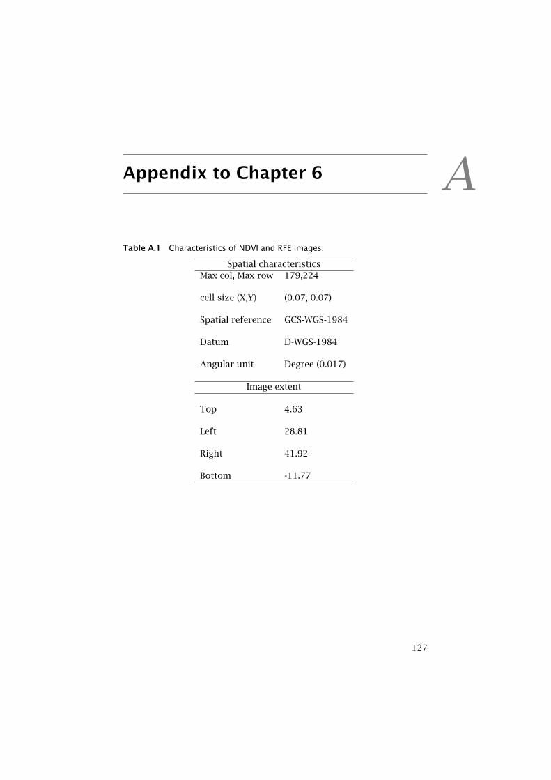
AAppendix to Chapter 6
Table A.1 Characteristics of NDVI and RFE images.
Spatial characteristicsMax col, Max row 179,224
cell size (X,Y) (0.07, 0.07)
Spatial reference GCS-WGS-1984
Datum D-WGS-1984
Angular unit Degree (0.017)
Image extent
Top 4.63
Left 28.81
Right 41.92
Bottom -11.77
127
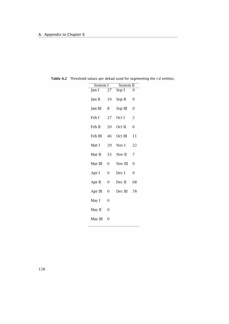
A. Appendix to Chapter 6
Table A.2 Threshold values per dekad used for segmenting the rd entities.
Season I Season IIJan I 27 Sep I 0
Jan II 10 Sep II 0
Jan III 8 Sep III 0
Feb I 27 Oct I 2
Feb II 20 Oct II 6
Feb III 46 Oct III 11
Mar I 29 Nov I 22
Mar II 33 Nov II 7
Mar III 0 Nov III 0
Apr I 0 Dec I 0
Apr II 0 Dec II 68
Apr III 0 Dec III 78
May I 0
May II 0
May III 0
128
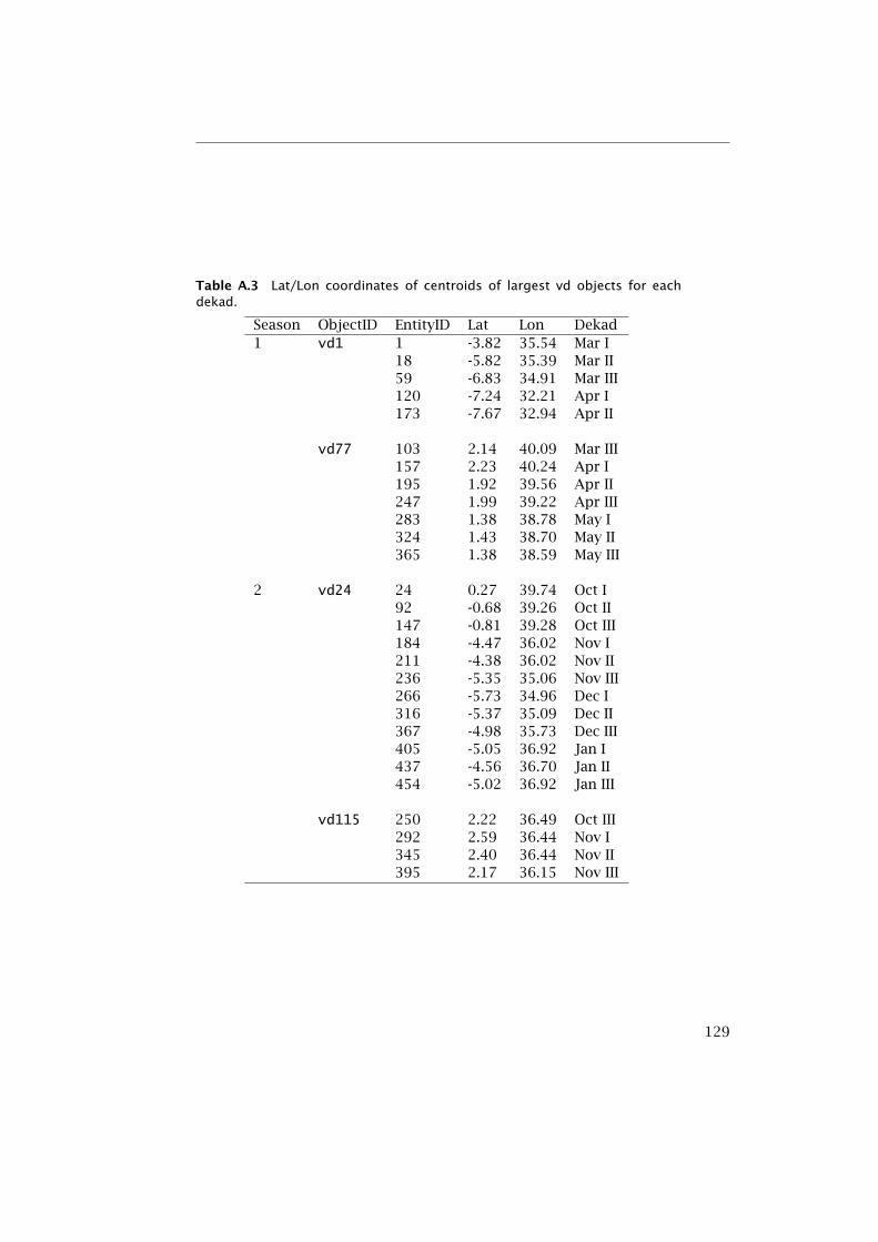
Table A.3 Lat/Lon coordinates of centroids of largest vd objects for eachdekad.
Season ObjectID EntityID Lat Lon Dekad1 vd1 1 -3.82 35.54 Mar I
18 -5.82 35.39 Mar II59 -6.83 34.91 Mar III120 -7.24 32.21 Apr I173 -7.67 32.94 Apr II
vd77 103 2.14 40.09 Mar III157 2.23 40.24 Apr I195 1.92 39.56 Apr II247 1.99 39.22 Apr III283 1.38 38.78 May I324 1.43 38.70 May II365 1.38 38.59 May III
2 vd24 24 0.27 39.74 Oct I92 -0.68 39.26 Oct II147 -0.81 39.28 Oct III184 -4.47 36.02 Nov I211 -4.38 36.02 Nov II236 -5.35 35.06 Nov III266 -5.73 34.96 Dec I316 -5.37 35.09 Dec II367 -4.98 35.73 Dec III405 -5.05 36.92 Jan I437 -4.56 36.70 Jan II454 -5.02 36.92 Jan III
vd115 250 2.22 36.49 Oct III292 2.59 36.44 Nov I345 2.40 36.44 Nov II395 2.17 36.15 Nov III
129
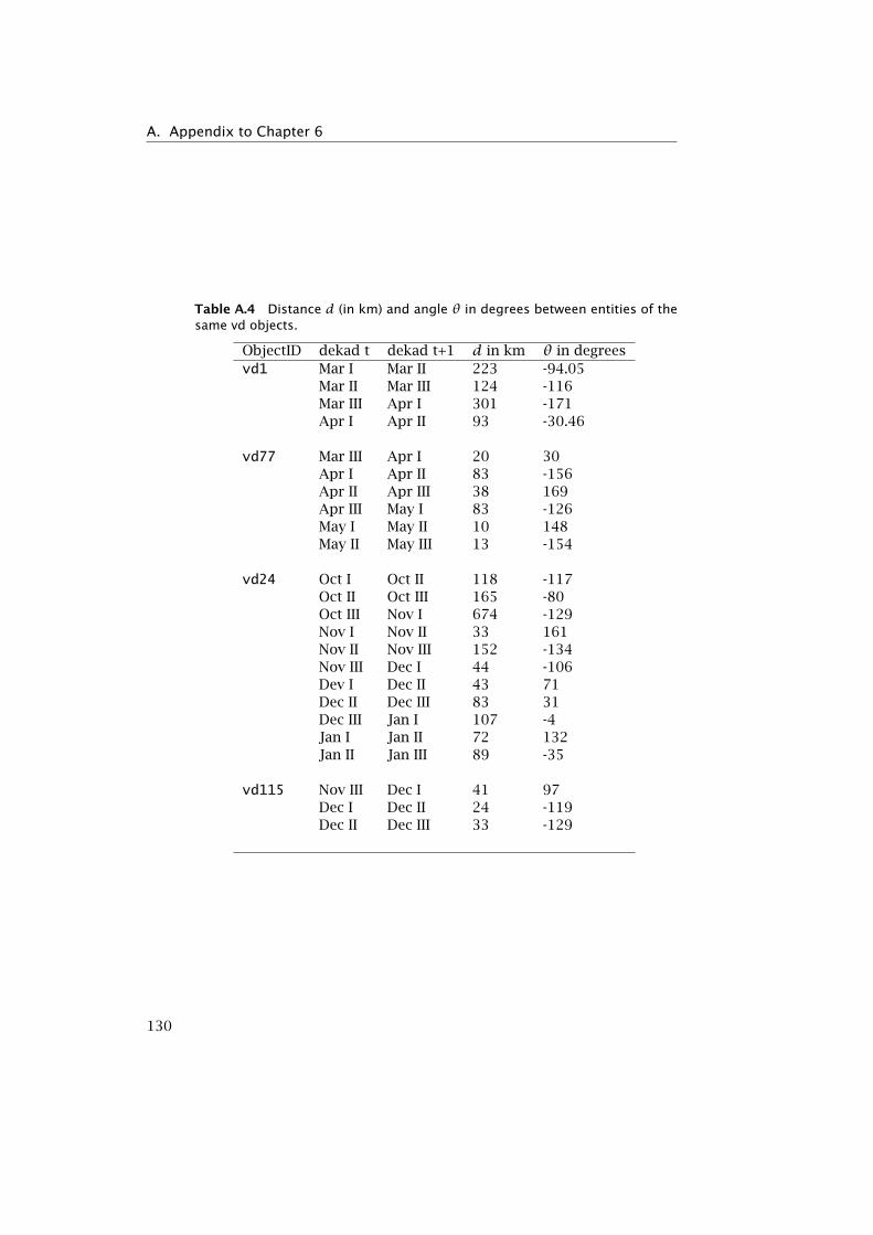
A. Appendix to Chapter 6
Table A.4 Distance d (in km) and angle θ in degrees between entities of thesame vd objects.
ObjectID dekad t dekad t+1 d in km θ in degreesvd1 Mar I Mar II 223 -94.05
Mar II Mar III 124 -116Mar III Apr I 301 -171Apr I Apr II 93 -30.46
vd77 Mar III Apr I 20 30Apr I Apr II 83 -156Apr II Apr III 38 169Apr III May I 83 -126May I May II 10 148May II May III 13 -154
vd24 Oct I Oct II 118 -117Oct II Oct III 165 -80Oct III Nov I 674 -129Nov I Nov II 33 161Nov II Nov III 152 -134Nov III Dec I 44 -106Dev I Dec II 43 71Dec II Dec III 83 31Dec III Jan I 107 -4Jan I Jan II 72 132Jan II Jan III 89 -35
vd115 Nov III Dec I 41 97Dec I Dec II 24 -119Dec II Dec III 33 -129
130
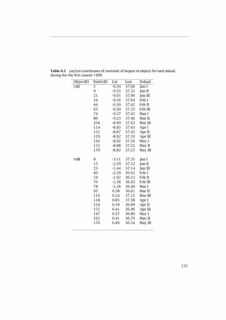
Table A.5 Lat/Lon coordinates of centroids of largest rd objects for each dekad,during the the first season 1999.
ObjectID EntityID Lat Lon Dekadrd2 2 -9.30 37.66 Jan I
9 -9.55 37.33 Jan II21 -9.05 37.90 Jan III34 -9.16 37.64 Feb I44 -9.30 37.42 Feb II63 -9.30 37.35 Feb III74 -9.27 37.42 Mar I86 -9.23 37.46 Mar II104 -8.99 37.43 Mar III114 -8.85 37.43 Apr I121 -8.87 37.43 Apr II129 -8.92 37.33 Apr III142 -8.92 37.26 May I155 -8.88 37.22 May II170 -8.82 37.25 May III
rd8 8 -3.11 37.35 Jan I13 -2.59 37.52 Jan II23 -1.44 37.14 Jan III40 -2.39 36.92 Feb I54 -1.92 36.12 Feb II70 -2.58 36.45 Feb III78 -1.28 36.40 Mar I93 0.38 36.61 Mar II110 0.24 37.15 Mar III118 0.85 37.38 Apr I124 0.18 36.89 Apr II135 0.41 36.96 Apr III147 0.37 36.80 May I162 0.41 36.70 May II176 0.49 36.54 May III
131
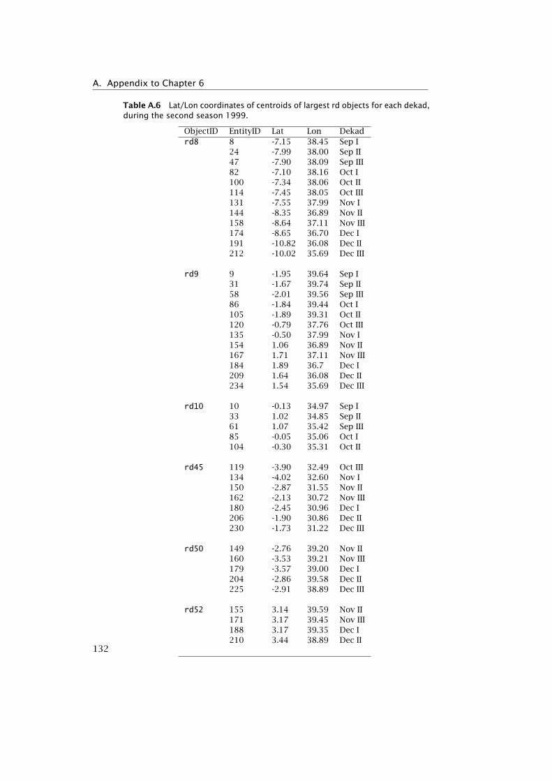
A. Appendix to Chapter 6
Table A.6 Lat/Lon coordinates of centroids of largest rd objects for each dekad,during the second season 1999.
ObjectID EntityID Lat Lon Dekadrd8 8 -7.15 38.45 Sep I
24 -7.99 38.00 Sep II47 -7.90 38.09 Sep III82 -7.10 38.16 Oct I100 -7.34 38.06 Oct II114 -7.45 38.05 Oct III131 -7.55 37.99 Nov I144 -8.35 36.89 Nov II158 -8.64 37.11 Nov III174 -8.65 36.70 Dec I191 -10.82 36.08 Dec II212 -10.02 35.69 Dec III
rd9 9 -1.95 39.64 Sep I31 -1.67 39.74 Sep II58 -2.01 39.56 Sep III86 -1.84 39.44 Oct I105 -1.89 39.31 Oct II120 -0.79 37.76 Oct III135 -0.50 37.99 Nov I154 1.06 36.89 Nov II167 1.71 37.11 Nov III184 1.89 36.7 Dec I209 1.64 36.08 Dec II234 1.54 35.69 Dec III
rd10 10 -0.13 34.97 Sep I33 1.02 34.85 Sep II61 1.07 35.42 Sep III85 -0.05 35.06 Oct I104 -0.30 35.31 Oct II
rd45 119 -3.90 32.49 Oct III134 -4.02 32.60 Nov I150 -2.87 31.55 Nov II162 -2.13 30.72 Nov III180 -2.45 30.96 Dec I206 -1.90 30.86 Dec II230 -1.73 31.22 Dec III
rd50 149 -2.76 39.20 Nov II160 -3.53 39.21 Nov III179 -3.57 39.00 Dec I204 -2.86 39.58 Dec II225 -2.91 38.89 Dec III
rd52 155 3.14 39.59 Nov II171 3.17 39.45 Nov III188 3.17 39.35 Dec I210 3.44 38.89 Dec II
132
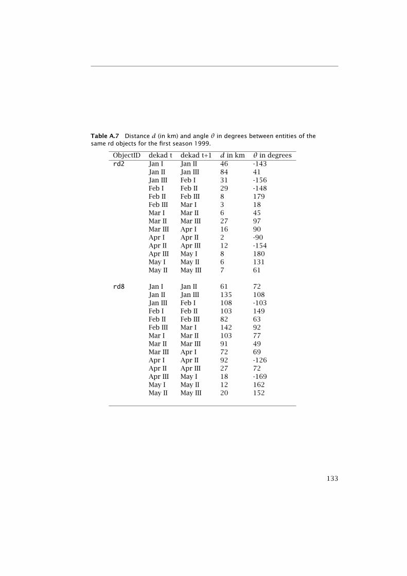
Table A.7 Distance d (in km) and angle θ in degrees between entities of thesame rd objects for the first season 1999.
ObjectID dekad t dekad t+1 d in km θ in degreesrd2 Jan I Jan II 46 -143
Jan II Jan III 84 41Jan III Feb I 31 -156Feb I Feb II 29 -148Feb II Feb III 8 179Feb III Mar I 3 18Mar I Mar II 6 45Mar II Mar III 27 97Mar III Apr I 16 90Apr I Apr II 2 -90Apr II Apr III 12 -154Apr III May I 8 180May I May II 6 131May II May III 7 61
rd8 Jan I Jan II 61 72Jan II Jan III 135 108Jan III Feb I 108 -103Feb I Feb II 103 149Feb II Feb III 82 63Feb III Mar I 142 92Mar I Mar II 103 77Mar II Mar III 91 49Mar III Apr I 72 69Apr I Apr II 92 -126Apr II Apr III 27 72Apr III May I 18 -169May I May II 12 162May II May III 20 152
133
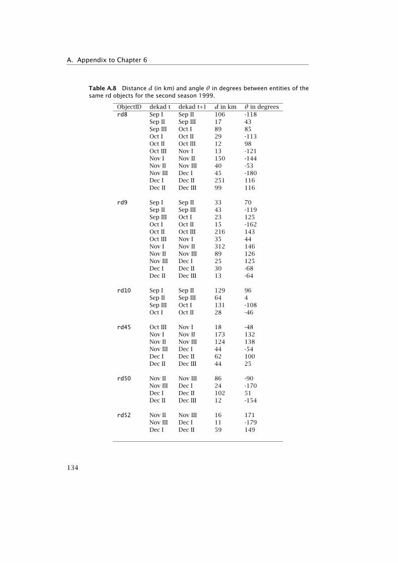
A. Appendix to Chapter 6
Table A.8 Distance d (in km) and angle θ in degrees between entities of thesame rd objects for the second season 1999.
ObjectID dekad t dekad t+1 d in km θ in degreesrd8 Sep I Sep II 106 -118
Sep II Sep III 17 43Sep III Oct I 89 85Oct I Oct II 29 -113Oct II Oct III 12 98Oct III Nov I 13 -121Nov I Nov II 150 -144Nov II Nov III 40 -53Nov III Dec I 45 -180Dec I Dec II 251 116Dec II Dec III 99 116
rd9 Sep I Sep II 33 70Sep II Sep III 43 -119Sep III Oct I 23 125Oct I Oct II 15 -162Oct II Oct III 216 143Oct III Nov I 35 44Nov I Nov II 312 146Nov II Nov III 89 126Nov III Dec I 25 125Dec I Dec II 30 -68Dec II Dec III 13 -64
rd10 Sep I Sep II 129 96Sep II Sep III 64 4Sep III Oct I 131 -108Oct I Oct II 28 -46
rd45 Oct III Nov I 18 -48Nov I Nov II 173 132Nov II Nov III 124 138Nov III Dec I 44 -54Dec I Dec II 62 100Dec II Dec III 44 25
rd50 Nov II Nov III 86 -90Nov III Dec I 24 -170Dec I Dec II 102 51Dec II Dec III 12 -154
rd52 Nov II Nov III 16 171Nov III Dec I 11 -179Dec I Dec II 59 149
134
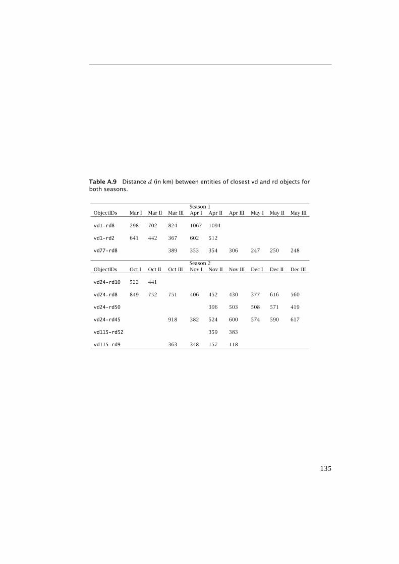
Table A.9 Distance d (in km) between entities of closest vd and rd objects forboth seasons.
Season 1ObjectIDs Mar I Mar II Mar III Apr I Apr II Apr III May I May II May III
vd1-rd8 298 702 824 1067 1094
vd1-rd2 641 442 367 602 512
vd77-rd8 389 353 354 306 247 250 248
Season 2ObjectIDs Oct I Oct II Oct III Nov I Nov II Nov III Dec I Dec II Dec III
vd24-rd10 522 441
vd24-rd8 849 752 751 406 452 430 377 616 560
vd24-rd50 396 503 508 571 419
vd24-rd45 918 382 524 600 574 590 617
vd115-rd52 359 383
vd115-rd9 363 348 157 118
135

Bibliography
Altman, D. (1994). Fuzzy set theoretic approaches for handling impreci-sion in spatial analysis. International Journal of Geographical InformationSystems, 8:271 – 289.
Ambenje, P. (2000). Proceedings of an expert group meeting. In EarlyWarning Systems for Drought Preparedness and Drought Management: Re-gional Drought Monitoring Centres: The Case of Eastern and Southern Africa,Lisbon, Portugal.
Anderson, T. and Goodman, L. (1957). Statistical inference about Markovchains. The annals of Mathematical Statistics, 28(1):98 – 110.
Anyamba, A. and Tucker, C. (2005). Analysis of Sahelian vegetationdynamics using NOAA-AVHRR NDVI data from 1981 U 2003. Journal ofArid Environments, 63:596 – 614.
Anyamba, A. and Tucker, C. (2011). NDVI anomaly patterns over Africaduring the 1997/98 ENSO warm event. International Journal of RemoteSensing, 22:1847 – 1859.
Bajgirana, P., Darvishsefat, A., Khalilic, A., and Makhdoumd, M. (2008).Using AVHRR-based vegetation indices for drought monitoring in theNorthwest of Iran. Journal of Arid Environments, 72:1086 – 1096.
Balzter, H. (2000). Markov chain models for vegetation dynamics. Ecolo-gical Modelling, 126:139 – 154.
Banik, P., Mandal, A., and Rahman, M. (2002). Markov chain analysisof weekly rainfall data in determining drought-proneness. DiscreteDynamics in Nature and Society, 7:231 – 239.
Barron, J., Rockstrom, J., Gichuki, F., and Hatibu, N. (2003). Dry spellanalysis and maize yields for two semi-arid locations in East Africa.Agricultural and Forest Meteorology, 117:23 – 37.
Bezdek, J. (1981). Pattern recognition with fuzzy objective function algorithms.New York, Plenum Press.
Bickenbach, F. and Bode, E. (2003). Evaluating the Markov property instudies of economics convergence. International Regional Science Review,26(3):363 – 392.
Bijker, W. (2007). Diurnal variation in NDVI : implications for seasonalland long-term changes. In 4th International workshop on the analysis ofmulti-temporal remote sensing images, Leuven, Belgium.
137
Bibliography
Blaschke, T. (2010). Object based image analysis for remote sensing.ISPRS Journal of Photogrammetry and Remote Sensing, 65(1):2 – 16.
Blaschke, T., Johansen, K., and Tiede, D. (2011). Advances in EnvironmentalRemote Sensing: Sensors, Algorithms, and Applications, chapter Objectbased image analysis for vegetation mapping and monitoring, pages245 – 276. Boca Raton, FL: CRC Press.
Blaschke, T., Lang, S., and Hay, G., editors (2008). Object-Based ImageAnalysis Spatial Concepts for Knowledge-Driven Remote Sensing ApplicationsSeries. Lecture Notes in Geoinformation and Cartography, Springer.
Bradfield, L. (2011). The recent decline of the long rains in East Africa. In91st American Meteorological Societe Annual Meeting.
Brown, D. (1998). Classification and boundary vagueness in mapping pre-settlement forest types. International Journal of Geographical InformationScience, 12:105 – 129.
Burrough, P. (1989). Fuzzy mathematical methods for soil survey andland evaluation. Journal of Soil Science, 40:477 – 492.
Chandrasekar, K., Sesha Sai, M., Roy, P., and Dwevedi, R. (2010). Landsurface water index (LSWI) response to rainfall and NDVI using theMODIS vegetation index product. International Journal of Remote Sensing,31(15):3987 – 4005.
Chatfield, C. (2004). The analysis of Time series: an introduction, volume 6 ofLectures Notes in Computer Sciences, chapter Autoregressive processes.Boca Raton: Chapman & Hall/CRC.
Cheng, T. and Molenaar, M. (2009). Objects with fuzzy spatial extent.Photogrammetric Engineering and Remote Sensing, 65(7):797 – 801.
Cheng, T., Molenaar, M., and Bouloucos, T. (1997). Spatial informationtheory: a theoretical basis for GIS, chapter Identification of Fuzzy Objectsfrom Field Observation Data, pages 241 – 259. Lectures Notes inComputer Sciences. Spring-Verlag, Berlin.
Cheng, T., Molenaar, M., and Lin, H. (2001). Formalization and applicationof fuzzy objects. International Journal of Geographical Information Science,15(1):27 – 42.
Cheng, T., Molenaar, M., and Stein, A. (2009). Remote Sensing and GeospatialTechnologies for Coastal Ecosystem Assessment and Management, chapterFuzzy Approach for Integrated Costal Zone management, pages 67 –90. Lecture Notes in Geoinformation and Cartography. Springer BerlinHeidelberg.
Comber, A., Wadsworth, R., and Fisher, P. (2006). Fundamentals of spatialdata quality, chapter 7, pages 123 – 139. Geographical informationsystems. ISTE.
Cooper, P., Dimes, J., Rao, K., Shapiro, B., and Twomlow, S. (2008). Copingbetter with current climatic variability in the rain-fed farming systemsof Sub-Saharan Africa: An essential first step in adapting to futureclimate change? Agriculture, Ecosystems & Environment, 126(1 - 2):24 –35.
138
Bibliography
Davenport, M. and Nickolson, S. (1993). On the relation between rainfalland Normalized Difference Vegetation Index for diverse vegetationtypes in East Africa. International Journal of Remote Sensing, 14(12):2369– 2389.
de Jong, S., Hornstra, T., and Maas, H. (2001). An integrated spatial andspectral approach to the classification of Mediterranean land covertypes: the SSC method. International Journal of Applied Earth Observationand Geoinformation, 3(2):176 – 183.
Devillers, R. and Jeansoulin, R. (2006). Fundamentals of spatial data quality,chapter Spatial data quality: concepts, pages 31 – 42. Geographicalinformation systems series. ISTE.
Dilo, A. (2006). Representation of and Reasoning with Vagueness in SpatialInformation. PhD thesis, ITC and Wageningen University.
Dilo, A., de By, R., and Stein, A. (2007a). Metrics for vague spatial objectsbased on the concept of mass. In Proceedings of 2007 IEEE InternationalConference on Fuzzy Systems, pages 804 – 809, Imperial College, London.IEEE Computational Intelligence Society.
Dilo, A., de By, R., and Stein, A. (2007b). A system of types and operatorsfor handling vague spatial objects. International Journal of GeographicalInformation Science, 21(4):397 – 426.
Ding, S., Rulinda, C., Stein, A., and Bijker, W. (2011). NDVI time series andMarkov chains to model the change of vegetative drought classes. InBruzone, L., Bovolo, F. I. o. E., and (IEEE), E. E., editors, 6th internationalworkshop on the analysis of multi-temporal remote sensing images, Multi-Temps, proceedings, Trento Italy.
Diouf, A. and Lambini, E. (2001). Monitoring land-cover changes in semi-arid regions: remote sensing data and field observations in the Ferlo,Senegal. Journal of Arid Environments, 48:129 – 148.
Dracup, A., Lee, K., and Paulson, E. (1980). On the definition of droughts.Water Resources Research, 16(2):291 – 302.
Drakopoulos, J. (1995). Probabilities, possibilities, and fuzzy sets. Fuzzysets and systems, 75(1):1 – 15.
EAC (2010). East african community. http://www.eac.int/.
EC-JRC-GEMU (2000). Global land cover 2000.http://bioval.jrc.ec.europa.eu/products/glc2000/glc2000.php.
Eklundh, L. (1996). AVHRR NDVI for monitoring and mapping vegetation anddrought in East Africa environments. PhD thesis, Lund University.
Eklundh, L. (1998). Estimating relations between AVHRR NDVI andrainfall in East Africa at 10-day and monthly time scales. InternationalJournal of Remote Sensing, 19(3):563 – 570.
EM-DAT (2011). the international disaster database.http://www.emdat.be/.
FAO/GIEWS (1999). Food outlook. Technical Report 5, FAO/GIEWS.http://www.fao.org/docrep/004/x3582e/x3582e07.htm#P722_15990.
139
Bibliography
Fensholt, R., Sandhot, I., Stisen, S., and Tucker, C. (2006). Vegetationmonitoring with the geostationary Meteosat Second Generation SEVIRIsensor. Remote Sensing of Environment, 101:212 – 229.
FEWSNETa (2006). Rwanda food security update. www.fews.net.
FEWSNETb (2006). Africa: Weather hazards assessment: 2-8 feb 2006.www.fews.net.
FEWSNETb (2011). FEWSNET weather hazards impacts assessment forAfrica. www.fews.net.
FEWSNETc (2005). Kenya food security update. www.fews.net.
FEWSNETd (2005). Rwanda food security update. www.fews.net.
FEWSNETf (2005). Africa: Weather hazards assessment: 15-21 december2005. www.fews.net.
Fisher, P. (2000). Sorites paradox and vague geographies. Fuzzy Sets andSystems, 12:47 – 62.
Fisher, P., Comber, A., and Wadsworth, R. (2006). Fundamentals of spatialdata quality, chapter Approaches to uncertainty in spatial data, pages43 – 59. ISTE.
Foody, G. (1996). Approaches to the production and evaluation offuzzy land cover classification from remotely-sensed data. Interna-tional Journal of Remote Sensing, 17:1317 – 1340.
Frank, A. (2008). Analysis of dependence of decision quality on dataquality. Journal of Geographical Systems, 10(1):71 – 88.
Gao, B.-C. (1996). NDWI – a normalized difference water index for re-mote sensing of vegetation liquid water from space. Remote Sensing ofEnvironment, 58:257 – 268.
Gommes, R. and Petrassi, F. (1994). Rainfall variability and droughtin Sub-Saharan Africa since 1960. Technical Report 9, FAO/GIEWS.http://www.fao.org/waicent/faoinfo/sustdev/EIdirect/EIan0004.htm.
Gouvia, C., Trigo, R., and DaCamara, C. (2009). Drought and vegetationstress monitoring in Portugal using satellite data. Natural Hazards andEarth System Sciences, 9:185 – 195.
Gu, Y., Brown, J., Verdin, J., and Wardlow, B. (2007). A five-year analysisof MODIS NDVI and NDWI for grassland drought assessment over thecentral great plains of the United States. Geophysical Research Letters,34.
Gu, Y., Hunt, E., Wardlow, B., Basara, J., Brown, J., and Verdin, J. (2008).Evaluation of MODIS NDVI and NDWI for vegetation drought monitor-ing using Oklahoma Mesonet soil moisture data. Geophysical ResearchLetters, 35.
Hastenrath, S. (2001). Variations of East African climate during the pasttwo centuries. Climate Change, 50:209 – 217.
Herman, S., Anyamba, S., and Tucker, C. (2005). Recent trends in vegeta-tion dynamics in the African Sahel and their relationship to climate.Global Environment Changes, 15:394 – 404.
140
Bibliography
Holben, B. (1986). Characteristics of maximum-value composite imagesfor temporal AVHRR data. International Journal of Remote Sensing, 7:1435– 1445.
IMWI (2010). IWMI drought information center: Understanding drought.Technical report, International Water Management Institute.
Ji, L. and Peters, A. (2003). Assessing vegetation response to drought inthe Northern Great Plains using vegetation and drought indices. RemoteSensing of Environment, 87:85 – 98.
Jones, H. and Vaughan, R., editors (2010). Remote sensing of vegetation:Principles, techniques, and applications. Spectral indices. Oxford UniversityPress.
Kanjilal, V., Liu, H., and Schneider, M. (2010). 13th International Confer-ence on Information Processing and Management of Uncertainty, IPMU 2010,volume 6178 LNAI of Lecture Notes in Computer Science, chapter Plat-eau regions: An implementation concept for fuzzy regions in spatialdatabases and GIS, pages 624 – 633. Springer, Heidelberg.
Klir, G. and Yuan, B. (1995). Fuzzy Sets and Fuzzy logic: Theory and Applica-tion. Prentice-Hall, New Jersey.
Kogan, F. (2001). Operational space technology for global vegetationassessment. Remote Sensing of Environment, 82:1949 – 1964.
Kraak, M.-J. and MacEachren, A. (1999). Visualization for exploration ofspatial data. first editorial of a special issue. International Journal ofGeographical Information Science, 13:285 – 287.
Kundzewicz, Z. (1997). Water resources for sustainable development.Hydrological Sciences Journal, 42(4):467 – 480.
Lacaze, B. and Bergés, J.-C. (2005). Contribution of Meteosat SecondGeneration (MSG) to drought early warning. In Proceedings of the Inter-national Conference: Remote Sensing and Geoinformation Processing in theAssessment and Monitoring of Land Degradation and Desertification: State ofthe Art and Operational Perspectives, Trier, Germany.
Leelaruban, N., Akyuz, A., Oduor, P., and Padmanabhan, G. (2010). Geo-spatial analysis of drought impact and severity in North Dakota, USAusing remote sensing and GIS. In American Meteorological Society: 18th
Conference on Applied Climatology.
Liu, W. and Kogan, F. (1996). Monitoring regional drought using theVegetation Condition Index. International Journal of Remote Sensing,17(14):2761 – 2782.
Lucieer, A. and Kraak, M.-J. (2004). Interactive and visual fuzzy clas-sification of remotely sensed imagery for exploration of uncertainty.International Journal of Geographical Information Science, 18:491 – 512.
Maathuis, B., Gieske, A., Restios, B., Hendrikse, J., and Leeuwen, B. (2005).MSG data retriever: Tool for converting raw MSG SEVIRI L 1.5 files intoraster-GIS or raster image file format. ITC, Enschede, The Netherlands.
141
Bibliography
Matis, J., Saito, T., Grand, W., Iwig, W., and Richie, J. (1985). A Markovchain approach to crop yield forecasting. Agricultural systems, 18:171 –187.
Metternicht, G. (1999). Change detection assessment using fuzzy setsand remotely sensed data: an application of topographic map revision.ISPRS Journal of Photogrammetry and Remote Sensing, 4:221 – 223.
Metternicht, G. (2001). Assessing temporal and spatial changes of salinityusing fuzzy logic, remote sensing and GIS: foundations of an expertsystem. Ecological Modelling, 144(2 - 3):163 – 179.
Meyn, S. and Tweedie, R. (1993). Markov Chains and Stochastic Stability,chapter 2, pages 24 – 56. Springer-Verlag.
Miao, Z., Liu, Y., and Wang, H. (2005). Fuzzy-Markov chain model withweights for prediction of cultivated land demand. Geomatics and Inform-ation Science of Wuhan University, 30:305 – 308.
MINAGRI (2009). Farming. Technical report, Ministry of Agriculture andAnimal Resources.
Mishra, A. and Desai, V. (2005). Drought forecasting using stochasticmodels. Stochastic Environment Research and Risk Assessment, 19:326 –339.
Mishra, A. and Desai, V. (2009). Drought characterization: a probabilisticapproach. Stochastic Environment Research and Risk Assessment, 23:41 –55.
Mokhtari, A., Mansor, S., Mahmud, A., and Helmi, Z. (2011). Monitoringthe impacts of drought on land use/cover: A developed object-basedalgorithm for NOAA AVHRR time series data. Journal of Applied Sciences,11:3089 – 3103.
Molenaar, M. (1998). An introduction to the theory of spatial object modellingfor GIS. Taylor & Francis.
Morwood, J., editor (1995). The Pocket Oxford Latin Dictionary. Oxford.
Moulin, S., Bondeau, A., and Delecolle, R. (1998). Combining agriculturalcrop models and satellite observation: from field to regional scales.International Journal of Remote Sensing, 19:1021 – 1036.
Murad, H. and Islam Saiful, A. (2011). Drought assessment using remotesensing and GIS in North-West region of Bangladesh. In 3rd internationalconference on water & flood management (ICWFM).
Myneni, R. and Asrar, G. (1994). Atmospheric effects and spectral vegeta-tion indices. Remote Sensing of Environment, 47(3):390 – 402.
NCDC (2010). NCDC geodata portal. Technical report, NOAA’s Nationalclimatic data centre. http://gis.ncdc.noaa.gov/.
Nguyen, T., Peterson, J., Gordon-Brown, L., and Wheeler, P. (2008). Coastalchanges predictive modelling: a fuzzy set approach. World Academy ofScience, Engineering and Technology, 48.
142
Bibliography
Nicholson, S. (1994). Recent rainfall fluctuations in Africa and their rela-tionship to past conditions over the continent. The Holocene, 4(2):121 –134.
Nicholson, S. (2000). The nature of rainfall variability over Africa on timescales of decades to millenia. Global and Planetary Change, 26:137 – 158.
Nicholson, S., Davenport, M., and Malo, A. (1990). A comparison ofthe vegetation response to rainfall in the Sahel and East Africa, usingnormalized difference vegetation index from NOAA-AVHRR. Climaticchange, 17:209 – 241.
Olsson, L., Eklundh, L., and Ard, J. (2005). A recent greening of the Sahel– trends, patterns and potential causes. Journal of Arid Environment,63:556 – 566.
Pantuliano, S. and Pavanello, S. (2009). Taking drought into accountaddressing chronic vulnerability among pastoralists in the Horn ofAfrica. HPG Policy Briefs, 35.
Panu, U. and Sharma, T. (2002). Challenges in drought research: someperspectives and future directions. Hydrological Sciences. Special issue:Towards integrated water resources management for sustainable development,S47.
Paulo, A. and Ferreira, E. (2007). Prediction of SPI drought class trans-itions using Markov chains. Water Resources Management, 21:1813 –1827.
Paulo, A., Ferreira, E., Coelho, C., and Pereira, L. (2005). Drought classtransition analysis through Markov and Loglinear models, an approachto early warning. Agricultural Water Management. Special issue on Land andWater Use: Environmental Management Tools and Practices, 77(1 - 3).
Pauly, A. and Schneider, M. (2010). VASA: An algebra for vague spatialdata in databases. Information Systems, 35:111 – 138.
Pereira, L., Cordery, I., and Iacovides, I. (2009). Coping with Water Scarcity.Springer Netherlands.
Peters, A., WalterShea, E., Ji, L., Viña, A., Hayes, M., and Svoboda, M.(2002). Drought monitoring with NDVI-based Standardized VegetationIndex. Photogrammetric Engineering & Remote Sensing, 68(1):71 – 75.
Pinzón, J., Brown, M., and Tucker, C. (2005). Hilbert-Huang transform:Introduction and Applications, chapter Satellite time series correction oforbital drift artifacts using empirical mode decomposition, pages 167– 186. World Scientific.
Purevdorj, T., Tatelshi, R., Ishiyama, T., and Honda, Y. (1998). Relation-ships between percent vegetation cover and vegetation indices. Interna-tional Journal of applied earth observation and geoinformation, 19(18):3519– 3535.
Quan, W. and Tenhunen, J. (2004). Vegetation mapping with multitem-poral NDVI in North Eastern China Transect (NECT). International Journalof applied earth observation and geoinformation, 6(1):17 – 31.
143
Bibliography
Retsios, B., Hendrikse, J., Gieske, A., van Leeuwen, B., and Maathuis, B.(2005). MSG data retriever, version 1.2. Technical report, ITC, Enschede,The Netherlands.
Robinson, V. (1988). Some implications of fussy set theory applied togeographic databases. Computers, Environment and Urban Systems, 12:89– 98.
Robinson, V. (2003). A perspective on the fundamentals of fuzzy setsand their use in geographic information systems. Transactions in GIS,7(1):3 – 30.
Rojas, O., Vrieling, A., and Rembold, F. (2011). Assessing drought prob-ability for agricultural areas in Africa with coarse resolution remotesensing imagery. Remote Sensing of Environement, 115:343 – 352.
Rossi, S. (2009). Remote sensing for drought monitoring. In 1st jointDMCSEE-JRC workshop on drought monitoring, Ljubljiana, 21-25 Septem-ber.
Rulinda, C., Bijker, W., and Stein, A. (2010). Image mining for droughtmonitoring in Eastern Africa using Meteosat SEVIRI data. InternationalJournal of Applied Earth Observation and Geoinformation, 12(1):S63 – S68.
Rulinda, C., Dilo, A., Bijker, W., and Stein, A. (2012). Characterising andquantifying vegetative drought in East Africa using fuzzy modelingand NDVI data. Journal of Arid Environment, 78:169 – 178.
Samtaney, R., Silver, D., Zabusky, N., and Cao, J. (1994). Visualizingfeatures and tracking their evolution. IEEE Computer, 27(7):20 – 27.
Sannier, C., Taylor, J., du Plessis, W., and Campbell, K. (1998). Realtime vegetation monitoring with NOAA-AVHRR in Southern Africafor wildlife management and food security assessment. InternationalJournal of Remote Sensing, 19(4):621 – 639.
Schneider, M. (1999). Advances in Spatial Databases, SSD’99, volume 1651 ofLecture Notes in Computer Science, chapter Uncertainty management forspatial data in databases: Fuzzy spatial data types, pages 330 – 351.Springer, Heidelberg.
Silver, D. and Wang, X. (1996). Volume tracking. In Yagel, R. and Neilson,G., editors, Seventh IEEE Visualization 1996 (VIS’96), pages 157 – 164,California, United States.
Sinclair (2005). Markov chains. Technical report, NDMC.
Sinnot, R. (1984). Virtues of the haversine. Sky and Telescope, 68(2):159.
Slegers, M. (2008). “if only it would rain”: Farmers perceptions of rainfalland drought in semi-arid central Tanzania. Journal of Arid Environment,72:2106 – 2123.
Smith, K. (2009). Environmental Hazards: assessing risk and reducing disaster,chapter Hydrological Hazards: Drought, pages 262 – 280.
Song, X., Saito, G., Kodama, M., and Sawada, H. (2004). Early detectionsystem of drought in East Asia using NDVI from NOAA/AVHRR data.International Journal of Remote Sensing, 25(16):3105 – 3111.
144
Bibliography
Stein, A., Hamm, N., and Qinghua, Y. (2009). Handling uncertainties inimage mining for remote sensing studies. International Journal of RemoteSensing, 30(20):5365 – 5382.
Swenson, S. and Wahr, J. (2009). Monitoring the water balance of lakeVictoria, East Africa, from space. Journal of Hydrology, 370:123 – 176.
Tan, B. and Yilmaz, K. (2002). Markov chain test for time dependenceand homogeneity: an analytical and empirical evaluation. EuropeanJournal of Operational Research, 137(3):524 – 543.
Thenkabail, P., Gamage, M., and Smakhtin, V. (2004). Use of remotesensing data for drought assessment and monitoring in SouthwestAsia. Technical Report 85, International Water Management Institute(IWMI).
Thorton, P., Jones, P., Alagarswamy, G., and Andresen, J. (2009). Spatialvariation of crop yield response to climate change in East Africa. GlobalEnvironmental Change, 19:54 – 65.
Tucker, C. (1979). Red and photographic infrared linear combinationsfor monitoring vegetation. Remote Sensing of Environment, 8:127 – 150.
Tucker, C. and Choudhury, B. (1987). Satellite remote sensing of droughtconditions. Remote Sensing of Environment, 23:243 – 251.
Tucker, C., Pinzón, J., Brown, M., Slayback, D., E.W., Pak, E., Mahoney,R., Vermote, E., and El Saleous, N. (2005). An extended AVHRR 8-kmNDVI data set compatible with MODIS and SPOT vegetation NDVI data.International Journal of Remote Sensing, 26(20):4485 – 4498.
Tucker, C. and Stenseth, N. (2005). Using the satellite-derived NDVI toassess ecological responses to environmental change. Trends in Ecology& Evolution, 20(9):503 – 510.
Turdukolov, U. (2007). Visualizing the evolution of image features in time-series: supporting the exploration of sensor data. PhD thesis, InternationalInstitute of Geoinformation Science and Earth Observation, UniversiteitUtrecht (UU-ITC).
Turdukulov, U., Block, C., Ruessink, B., and Turner, I. (2007). Connectingusers with their data: An environment to explore the morphodynamicsof rip channels. Cartographica, 42:139 – 151.
Turdukulov, U., Tolpekin, V., and Kraak, M.-J. (2005). Visual exploration oftime series of remote sensing data. In Spatial-temporal Modeling, SpatialReasoning, Analysis, Data Mining and Data Fusion (ISPRS-WG/II), Beijing,China 27-29 August, 2005.
UNEP/UNDP/GOR (2007). Pilot integrated ecosystem assessment ofBugesera. poverty and environment initiative project (PEI). Technical re-port, UNEP/UNDP/GOR. http://www.unpei.depiweb.org/PDF/Bugesera-Rwanda.pdf.
Unganai, L. and Kogan, F. (1998). Drought monitoring and corn yieldestimation in Southern Africa from AVHRR data. Remote sensing ofenvironment, 63(3):219 – 232.
145
Bibliography
UNICEF (2000). Drought in East Africa. Technical report, UNICEF.http://www.unicef.org/africadrought/.
Vlek, P., Le, Q., and Tamene, L. (2008). Land decline in land-rich Africa - acreeping disaster in the making. Technical report, Rome, Italy: CGIARScience Council Secretariat.
Wang, F. (1990). Improving remote sensing image analysis through fuzzyinformation representation. Photogrammetric Engineering and RemoteSensing, 56:1163 – 1169.
Whilite, D. and Glantz, M. (1987). Understainding the drought phe-nomenon: the role of definitions. Water International, pages 111 – 120.
Wilhite, D. (2005). Drought and water crisis: science, technology and manage-ment issues. Taylor & Francis Group.
Woodcock, E. and Gopal, S. (2000). Fuzzy set theory and thematic maps:accuracy assessment and area estimation. International Journal of Geo-graphical Information Science, 14(2):153 – 172.
WRI (2007). Nature’s Benefits in Kenya. An Atlas of Ecosystems and HumanWell-Being. World Resources Institute, Washington DC and Nairobi.
Xie, P. and Arkin, P. (1997). A 17-year monthly analysis based on gaugeobservations, satellite estimates, and numerical model outputs. Bulletinof the American Meteorological Society, 11:2539 – 2558.
Zadeh, L. (1965). Fuzzy sets. Information and Control, 8:338 – 353.
Zadeh, L. (1968). Probability measures of fuzzy events. Journal of Math-ematical Analysis and Applications, 23(2):421 – 427.
Zadeh, L. (1984). Fuzzy sets as a basis for a theory of possibility. FuzzySets and Systems, 1:3 – 28.
146

Biography
Coco G. Musaningabe Rulinda was born on February 9, 1979 in Kinshasa,Democratic Republic of Congo. From 1998, she studied in the Facultyof Applied Sciences, University of Rwanda (Rwanda), where she receivedher BSc. degree with distinction in Computer Science. After her studiesshe joined the Center for GIS and Remote Sensing (CGIS) of the NationalUniversity of Rwanda, where she worked as the IT officer. From 2005,she joined the department of Computer Science,Faculty of Applied Sciences, as an assistant lec-turer, while also being appointed as a trainer andresearch assistant at the CGIS. In 2005 she wasgranted a NPT/RWA/071 scholarship to pursueher MSc degree in Geo-Information Science andEarth Observation at ITC in Enschede, with a spe-cialization in geoinformatics. Her MSc thesis,completed with distinction, was on modelingdrought uncertainty using fuzzy set theory. FromSeptember 2007, she pursued a PhD researchwithin the same research context. Her researchinterests in remote sensing include uncertaintymodeling and spatiotemporal change analysis.
147


Author’s Publications
Published ISI Journal Articles
C.M. Rulinda, W. Bijker, A. Stein (2010). Image mining for drought monit-oring in Eastern Africa using Meteosat SEVIRI data. International Journal ofApplied Earth Observation and Geoinformation, 12 (Supp. 1), S63-S68.
C.M. Rulinda, A. Dilo, W. Bijker, A. Stein (2012). Characterizing andquantifying vegetative drought in East Africa using fuzzy modelling andNDVI data. Journal of Arid Environments, 78, 169-178.
ISI Journal Articles Under Review
C.M. Rulinda, S. Ding, W. Bijker, A. Stein. Modelling the dynamics ofvegetative drought area. International Journal of Remote Sensing.
C.M. Rulinda, A. Stein, U. Turdukulov. Visualizing and quantifying themovement of vegetative drought using remote sensing data and GIS.International Journal of Geographical Information Science.
Conference Papers
C.M. Rulinda, W. Bijker, A. Stein (2011). The chlorophyll variability inmeteosat derived NDVI in a context of drought monitoring. In: ProcediaEnvironmental Sciences, 3, 1st conference on Spatial Statistics 2011 -Mapping Global Change, Enschede, 23-25 March 2011.
S. Ding, C.M. Rulinda, A. Stein, W. Bijker (2011). NDVI time series andMarkov chains to model the change of vegetative drought classes. In:6th international workshop on the analysis of multi - temporal remotesensing images, Multi - Temp, proceedings, 12-14 July 2011, Trento, Italy/ ed. by L. Bruzozne and F. Bovolo: Institute of Electrical and ElectronicsEngineers (IEEE).
149

ITC dissertations
A complete list of ITC dissertations is online on the ITC website:
www.itc.nl/research/phd/phd_graduates.aspx.
151