A Memory-Efficient Finite Volume Method forAdvection-Diffusion-Reaction Systems withNon-Smooth SourcesJonas Schafer,1 Xuan Huang,2 Stefan Kopecz,1,0 Philipp Birken,1

Matthias K. Gobbert,2 and Andreas Meister1

1Institute of Mathematics, University of Kassel, 34132 Kassel, Germany2Department of Mathematics and Statistics, University of Maryland, Baltimore County, Baltimore,MD 21250, USA

We present a parallel matrix-free implicit finite volume scheme for the solution of unsteadythree-dimensional advection-diffusion-reaction equations with smooth and Dirac-Delta sourceterms. The scheme is formally second order in space and a Newton-Krylov method is employedfor the appearing nonlinear systems in the implicit time integration. The matrix-vector productrequired is hardcoded without any approximations, obtaining a matrix-free method that needslittle storage and is well suited for parallel implementation. We describe the matrix-free imple-mentation of the method in detail and give numerical evidence of its second order convergencein the presence of smooth source terms. For non-smooth source terms the convergence orderdrops to one half. Furthermore, we demonstrate the method’s applicability for the long timesimulation of calcium flow in heart cells and show its parallel scaling.

Keywords: Finite volume method; Dirac delta distribution; Matrix-free Newton-Krylov method;Calcium waves; Parallel computing

I INTRODUCTION

Advection-diffusion-reaction systems occur in a wide variety of applications, as for instance heattransfer or transport-chemistry problems. Long-time simulations of such real-life applicationsoften require implicit methods on very fine computational grids, to resolve the desired accuracy,especially in three dimensions. When performing such simulations with methods storing systemmatrices, the availability of memory becomes an issue already on relatively coarse meshes. Oneway to address this problem is the use of parallel methods, which distribute the workloadamong several CPUs and use the memory associated with these CPUs to solve larger systems.If this approach does not provide enough memory to obtain the desired resolution, parallelmatrix-free methods are an excellent choice, since in general most of the memory is used tostore system matrices. In addition, matrix-free methods require less communication comparedto classical schemes, thus these are more suited for use on parallel architectures and allow forbetter scalability.

To solve linear systems most matrix-free methods use Krylov subspace methods, whichonly require the results of matrix-vector products in every iteration. If these can be providedwithout storing the matrix, this leads to significant savings of memory and computations onhigh resolution meshes become feasible. A prominent example are Jacobian-free Newton Krylov(JFNK) methods, which approximate the Jacobian matrix by finite differences via functionevaluations [1]. In the following we present another type of matrix-free Newton-Krylov method,which provides the matrix-vector products with the exact Jacobian by hardcoding the product.This method is thus specific to a given class of equations and grids and particularly suitablefor computations on structured grids.

0Correspondence to: Stefan Kopecz, Institute of Mathematics, University of Kassel, Heinrich-Plett-Str. 40,34132 Kassel, Germany (e-mail: kopecz@mathematik.uni-kassel.de)

1

In [2] (see also [3] for details) a matrix-free Newton-Krylov method for the simulation ofcalcium flow in heart cells was presented. The underlying model of calcium flow is given bya system of three coupled diffusion-reaction equations, in which the occurring source termscan be divided into linear and nonlinear parts, as well as point sources. Due to the elongatedshape of a heart cell and the focus of the work on physiological parameter values, a rectangulardomain with a structured grid is a natural choice. The method is based on a finite elementdiscretization and implemented in a matrix-free manner. Good parallel scalability of the parallelimplementation was demonstrated in [2]. The convergence of the finite element method inpresence of measure valued source terms, as they occur in the calcium model, was rigorouslyshown in [4], and numerical results agree well with the theoretical predictions.

In this paper we show the performance of a formally second order finite volume schemein the framework of the matrix-free method from [2]. Since we intend to consider advectiondominated systems in the future, this is done for the more general class of equation systems ofadvection-diffusion-reaction (ADR) type. For this type of problems finite volume methods area natural choice as opposed to finite element methods which would need additional stabilizationterms [5]. Additionally, we deal with point sources generated by Dirac delta distributions, asthey occur in the calcium flow equations. There is very little convergence theory in this case. In[6], convergence of a finite volume method is shown for hyperbolic scalar conservation laws withpoint sources, but no order of convergence is proved. The negative-norm convergence order ofDG schemes for problems containing Dirac sources was investigated in [7].

In the absence of a general convergence theory we demonstrate convergence of the methodnumerically and compare the results to those obtained by the finite element method from [2],for which a rigorous convergence theory is available. To demonstrate the method’s powerin real life applications, we show results of long-time simulations of calcium flow in heartcells, the motivating application problem from [2]. Furthermore, a parallel performance studydemonstrates the good scalability of the parallel implementation and we show that the overallperformance of the finite volume scheme is comparable to the finite element method withcomparable errors and runtimes. As Krylov subspace method, BiCGSTAB is employed.

The outline of this paper is as follows. Section II introduces the system of ADR equationsand gives a short description of the equations modeling the calcium flow in heart cells as well asthe test cases that will be used to demonstrate the convergence of numerical method. In Sec-tion III we derive the finite volume method and describe its parallel matrix-free implementationin detail. In Section IV various convergence studies are presented to give numerical evidenceof the convergence of the finite volume scheme. This includes test cases with smooth and non-smooth source terms. Whenever possible, the results are compared to those obtained by thefinite element scheme of [2]. Section V illustrates the applicability of the method to long timesimulations of calcium in heart cells and compares the finite volume results to those obtainedby the finite element method. Finally, the scalability of the scheme in parallel computationswill be presented in Section VI.

II GOVERING EQUATIONS

We consider the three-dimensional system of advection-diffusion-reaction equations

u(i)t −∇ · (D

(i)∇u(i) − u(i)β(i)) + a(i)u(i) = q(i)(u(1), . . . , u(ns)) (2.1)

of i = 1, . . . , ns species with u(i) = u(i)(x, t) representing functions of space x ∈ Ω ⊂ R3

and time 0 < t ≤ tfin. Without loss of generality, the components of the constant ve-locity vectors β(i) ∈ R3 are non-negative. The entries of the diffusive diagonal matricesD(i) = diag (D(i)

11 , D(i)22 , D

(i)33 ) ∈ R3×3 are positive constants, and the reactive parameter a(i) ≥ 0

is a constant as well. The source terms q(i) represent different types of sources. In the follow-ing we consider source terms which depend on space and time solely, nonlinear reaction terms

2

depending on u(1), . . . , u(ns), and point sources containing Dirac delta distributions.To describe the problem completely initial conditions u(i)|t=0 = u

(i)ini as well as boundary

conditions on the domain’s boundary ∂Ω are necessary. We employ homogeneous Neumannboundary conditions D(i)∇u(i) · n = 0 for i = 1, . . . , ns, in which n is the outward pointingnormal vector on ∂Ω.

II.A Calcium Flow Model

Within the general system (2.1) a model for the calcium flow in heart cells is included, see [2]and the references therein for details. This model consists of ns = 3 equations corresponding tocalcium (i = 1), an endogenous calcium buffer (i = 2) and a fluorescent indicator dye (i = 3).It is obtained by neglecting advective effects, i.e. β(i) = 0 for i = 1, 2, 3, and setting

q(i)(u(1), u(2), u(3)) = r(i)(u(1), u(2), u(3)) + (−Jpump(u(1)) + Jleak + JSR(u(1)))δi1.

The reaction terms r(i) are nonlinear functions of the different species and couple the threeequations. Terms belonging only to the first equation are multiplied with the Kronecker deltafunction δi1. These are the nonlinear drain term Jpump, the constant balance term Jleak, andthe key of the model in JSR. This term, which is given by

JSR(u(1),x, t) =∑

x∈Ωs

σSx(u(1), t)δ(x− x),

models the release of calcium into the cell at special locations called calcium release units(CRUs). The indicator function Sx determines whether a CRU is open or not, σ controls theamount of calcium injected into the cell and Ωs represents the set of all CRUs. Furthermore,δ(x − x) denotes a Dirac delta distribution for a CRU located in x. Thus, JSR models thesuperposition of point sources at the locations of all CRUs. A complete list of the model’sparameter values is given in Table 2.1.

II.B Scalar Test Cases

In order to demonstrate the convergence of the method presented in Section III we will considera number of test cases, which are simplifications of the system (2.1) or the calcium model fromSection II.A, respectively.

II.B.1 ADR Equation with Smooth and Non-Smooth Source Term

The first test case is the unsteady scalar ADR equation (with superscript dropped)

ut −∇ · (D∇u) + β · ∇u+ au = f.

The domain and diffusive matrix D = D(1) are chosen as for the calcium model, see Table 2.1.The velocity is set to β = (0.1, 0.2, 0.3)T and the reactive parameter is a = 0.1. Thus, advection,diffusion and reaction are of equal order of magnitude.

With respect to the right hand side, we consider a smooth and a non-smooth f . In the firstcase, the initial condition uini and right hand side f are chosen such that

u(x, y, z, t) = (1/8)(1 + cos(λxx)e−Dxλ2xt)(1 + cos(λyy)e−Dyλ

2yt)(1 + cos(λzz)e−Dzλ

2zt) (2.2)

with λx = λy = π/6.4 and λz = π/32 is the true solution. To show the method’s convergenceeven in the presence of point sources, we also consider

f = σSx(t)δ(x− x),

3

Table 2.1: Parameters of the calcium flow model with ns = 3 species. The concentration unitM is short for mol/L (moles per liter).

Domains in space and timeΩ = (−6.4, 6.4)× (−6.4, 6.4)× (−32.0, 32.0) in units of µm0 < t ≤ tfin with tfin = 1,000 in units of ms

Advection-diffusion-reaction equationD(1) = diag(0.15, 0.15, 0.30) µm2 / msD(2) = diag(0.01, 0.01, 0.02) µm2 / msD(3) = diag(0.00, 0.00, 0.00) µm2 / msβ(i) = (0, 0, 0), a(i) = 0, f (i) ≡ 0 for all iu

(1)ini = 0.1 µM, u

(2)ini = 45.9184 µM, u

(3)ini = 111.8182 µM

CRU coefficients∆xs = 0.8 µm, ∆ys = 0.8 µm, ∆zs = 2.0 µmσ = 110.0 µM µm3, F = 96,485.3 C / mol (Faraday constant)Pmax = 0.3 / ms, Kprob = 2.0 µM, nprob = 4.0∆ts = 1.0 ms, topen = 5.0 ms, tclosed = 100.0 ms

Reaction termsk+

1 = 0.08 / (µM ms), k−1 = 0.09 / ms, u1 = 50.0 µMk+

2 = 0.10 / (µM ms), k−2 = 0.10 / ms, u2 = 123.0 µMPump and leak terms

Vpump = 4.0 µM / ms, Kpump = 0.184 µM, npump = 4Jleak = 0.320968365152510 µM / ms

with σ and uini = u(1)ini chosen as in Table 2.1. The intention is to simplify the calcium problem

by modelling a single CRU in the center of the domain, which opens at time t = 1 and remainsopen ever after. Therefore, we set x = (0, 0, 0) and

Sx(t) =

0, t < 1,1, t ≥ 1.

Numerical results with the smooth as well as the non-smooth source are shown in Section IV.B.

II.B.2 Diffusion with Homogeneous and Non-Smooth Source Term

To be able to compare finite volume results to those computed with the finite element schemefrom [2], we consider the test case from Section II.B.1 without advection. This means we setβ = 0 and a = 0 and obtain

ut −∇ · (D∇u) = f.

Again, we allow for the two different source terms, but due to the absence of advection andreaction the smooth source term, which is chosen such that the true solution is given by (2.2),becomes f = 0. See Section IV.A for the numerical results.

II.B.3 Pure Advection

Finally, we consider the linear advection equation

ut + β · ∇u = 0,

4

−6.40

6.4

−6.40

6.4

−32

−16

0

16

32

xy

z

−6.40

6.4

−6.40

6.4

−32

−16

0

16

32

xy

z

Figure 3.1: Regular mesh (left) and dual mesh (right).

with β = (1, 1, 1)T on the domain Ω = (0, 10) × (0, 10) × (0, 10). Since this is a hyperbolicproblem, we only need to specify boundary conditions on the inflow portion ∂Ωin ⊂ ∂Ω of theboundary. In this test case ∂Ωin is given by the intersection of ∂Ω with the (x,y), (x,z) and(y,z) hyperplanes and we assume homogeneous Neumann boundary conditions on ∂Ωin. Theproblem’s true solution is given by

u(x, y, z, t) = exp(−5((x− β1t− 2)2 + (y − β2t− 2)2 + (z − β3t− 2)2

)),

when starting with initial data uini(x, y, z) = u(x, y, z, 0). The numerical results of this testare shown in Section IV.C.

III NUMERICAL METHOD

In this section we describe the numerical method for the solution of the system of ADR equa-tions (2.1). In Section III.A the finite volume space discretization is explained. This alsoincludes a discussion of the treatment of Dirac delta sources. A brief description of the timeintegration and the matrix-free method is given in Section III.B and the matrix-free implemen-tation of the method is presented in detail in III.C. Finally, Section III.D discusses the parallelimplementation of the method.

III.A Space Discretization

To derive the finite volume discretization, let Th = K1, . . . ,KM be a mesh such that Ω =⋃Ml=1Kl. Each Kl ∈ Th is an open subset of Ω and referred to as cell or control volume.

Integration of (2.1) over an arbitrary cell Kl ∈ Th and application of the divergence theoremyields

d

dt

∫Kl

u(i) dx−∫∂Kl

(D(i)∇u(i) − u(i)β(i)) · nl ds+∫Kl

a(i)u(i) dx =∫Kl

q(i) dx, (3.1)

where ∂Kl denotes the boundary of Kl and nl its outward normal. This is the equation we areactually trying to solve, since it imposes less regularity on the solution. In particular, solutionswith discontinuities are now admissible. Denoting the volume of Kl by |Kl|, the spatial meanvalue of u(i) over Kl is given by

u(i)l (t) =

1|Kl|

∫Kl

u(i)(x, t) dx.

5

l + 1

l +Mx

l −MxMy

l+MxMy

l−Mx

l− 1

Figure 3.2: Control volume

With this notation, (3.1) can be rewritten as

d

dtu

(i)l −

1|Kl|

∫∂Kl

(D(i)∇u(i) − u(i)β(i)) · nl ds+ a(i)u(i)l =

1|Kl|

∫Kl

q(i) dx. (3.2)

This is a system of ordinary differential equations for the temporal evolution of the meanvalues u(i)

l . In this regard, the crucial part is the computation of the boundary fluxes in termsof neighboring mean values.

In the following we only consider brick shaped domains. Thus, it is convenient to discussthe flux approximation in a one-dimensional context and without species index i, which willthen be generalized to higher dimensions. Therefore, we condsider Ω = (Xmin, Xmax) and themesh

Th =Kl|Kl = (xl, xl+1), l = 1, . . . ,M

,

with x1 = Xmin and xM+1 = Xmax. The center of a cell Kl is given by ml = (1/2)(xl + xl+1).Since the superscripts (i), the right hand side and the reactive term, are of no importance forthe discussion of the flux approximation, we drop them and (3.2) can be written as

d

dtul −

1∆xl

(du′(xl+1)− βu(xl+1)− (du′(xl)− βu(xl))) = 0,

with ∆xl = xl+1 − xl.In order to approximate the advective flux βu(xl+1) by the mean values ul with l = 1, . . . ,M

we introduce a numerical flux function H = H(u+l , u

−l+1). The values u+

l and u−l+1 are approxi-mations to the unknown values of u on either side of xl+1. Assuming that β ≥ 0 as before, theupwind flux function for the advective flux is given by

Hupw(u+l , u

−l+1) = βu+

l . (3.3)

It respects the direction of velocity and thus avoids instabilities in purely advective situations.Assuming a constant distribution of u in Kl and Kl+1 leads to the definitions u+

l = ul andu−l+1 = ul+1. Using these values as input of the upwind flux function, results in a method of firstorder convergence. The order can be increased using a ENO or WENO approach and providinginput data based on a linear distribution of u within the cells. See [8] and the literature citedtherein for details on WENO schemes. Since we consider linear advection there is no differencebetween ENO and WENO and the input for the flux function is given by

u+l = ul +

ul − ul−1

ml −ml−1(xl+1 −ml). (3.4)

6

The choice of this particular linear distribution comes from the upwind idea that no informationto the right of xl+1 should be used in the flux computation. Note that the value of u−l+1 has noinfluence when using the upwind flux function (3.3).

To approximate the diffusive flux du′(xl+1), we use a central difference of the neighboringmean values and define the diffusive flux function as

Hdiff (ul, ul+1) = dul+1 − ulml+1 −ml

.

In this case, the mean values on either side of xl+1 are sufficient to obtain a scheme of secondorder.

So far, we have omitted the discussion of the homogeneous Neumann boundary conditions,which become du′(x1) = du′(xM+1) = 0 in this one-dimensional context. In particular, thecondition is equivalent to u′(x1) = u′(xM+1) = 0. The incorporation of this boundary conditionis done by setting Hdiff (u0, u1) = Hdiff (uM , uM+1) = 0 (or u0 = u1 and uM+1 = uM ,respectively). The situation becomes more delicate for the advective flux, where two criticalsituations occur. These are the computations of Hupw(u+

0 , u−1 ) and Hupw(u+

1 , u−2 ), for which

it is unclear how to choose the linear distribution in K1, since no Dirichlet data is availableat the boundary. The simple remedy which we are pursuing here, is the assumption of aconstant distribution in K1 and thus setting u+

1 = u1 in Hupw(u+1 , u

−2 ). Furthermore, we set

u+0 = u−1 = u1 in Hupw(u+

0 , u−1 ) to incorporate the boundary condition u′(x1) = 0. Note that

there are no difficulties with Hupw(u+M , u

−M+1), since u+

M can be computed from (3.4) withoutany problems and the chosen value of u−M+1 has no further influence.

Now, we extend this approach to three dimensions and define the mesh which is used forthe discretization. In [2] a regular mesh Ωh ⊂ Ω with constant mesh spacings ∆x, ∆y and∆z was used for the finite element space discretization. Here we employ the correspondingdual mesh Th, which is constructed by connecting all inner nodes of Ωh with lines parallelto the coordinate axes and extending these lines in a straight manner to the boundary. Thedual mesh is a rectilinear mesh and each inner node of Ωh is the center of a cell of Th withvolume ∆x∆y∆z. Furthermore, the volume of a cell is reduced to ∆x∆y∆z/2, ∆x∆y∆z/4or ∆x∆y∆z/8, whether this cell has a common face, edge or corner with the boundary ∂Ω.The exterior view on a typical regular mesh and the corresponding dual mesh is depicted inFigure 3.1. By construction the number of nodes of Ωh equals the number of cells in Th. Inthe following we assume that Th consists of M = MxMyMz control volumes, with Mx, My andMz denoting the number of cells in each direction and introduce the enumeration scheme

l = i+ (j − 1)Mx + (k − 1)MxMy (3.5)

for 1 ≤ i ≤Mx, 1 ≤ j ≤My and 1 ≤ k ≤Mz, which is indicated in Figure 3.2. Thus, a controlvolume Kl has the neighbors Kl−1 and Kl+1 in x-direction, Kl−Mx and Kl+Mx in y-directionand Kl−MxMy

and Kl+MxMyin z-direction.

For a given control volume Kl = (xL, xR) × (yL, yR) × (zL, zR) ∈ Th with spacings ∆xl =xR − xL,∆yl = yR − yL,∆zl = zR − zL the boundary fluxes from (3.2) can be written as∫

∂Kl

(D∇u− uβ) · nl ds

=∫ zR

zL

∫ yR

yL

(d11∂xu− β1u)|x=xR− (d11∂xu− β1u)|x=xL

dydz

+∫ zR

zL

∫ xR

xL

(d22∂yu− β2u)|y=yR− (d22∂yu− β2u)|y=yL

dxdz

+∫ yR

yL

∫ xR

xL

(d33∂zu− β3u)|z=zR− (d33∂zu− β3u)|z=zL

dxdy.

7

Here we exploited the fact, that the faces of Kl are parallel to the planes defined by thecoordinate axes and thus only one entry of the corresponding normal vectors is non-zero. Notealso that the superscripts (i) were dropped and that the above equation is valid for one of then species of the system. Using the midpoint rule and setting

Ha,j(uL, uR) = βj uL, Hd,j(uL, uR) = djjuR − uL|mR −mL|

, (3.6)

with mL and mR denoting the centers of the cells belonging to uL and uR, the boundary fluxescan be approximated as∫

∂Kl

(D∇u− uβ) · nl ds

≈ ∆yl∆zl(Hd,1(ul, ul+1)−Ha,1(u1,+

l , u1,−l+1)− (Hd,1(ul−1, ul)−Ha,1(u1,+

l−1, u1,−l ))

)+ ∆xl∆zl

(Hd,2(ul, ul+Mx

)−Ha,2(u2,+l , u2,−

l+Mx)− (Hd,2(ul−Mx

, ul)−Ha,2(u2,+l−Mx

, u2,−l ))

)+∆xl∆yl

(Hd,3(ul, ul+MxMy

)−Ha,3(u3,+l , u3,−

l+MxMy)− (Hd,3(ul−MxMy

, ul)−Ha,3(u3,+l−MxMy

, u3,−l ))

),

where the enumeration scheme (3.5) was used to describe the location of the input data of theflux functions. The notation uj,±l indicates that the approximation to the value of u lives inKl and belongs to the face which is between Kl and the element which lies in positive (+) ornegative (−) direction of the j-th coordinate. The computation of uj,±α and the treatment ofboundary conditions can be carried out as in the one-dimensional case.

The last step of the discretization is the treatment of the volume integral on the right handside of (3.2). This can be approximated sufficiently using the midpoint rule∫

Kl

q(x, t, u(1), . . . , u(n)) dx ≈ |Kl| q(ml, t, u(1)l , . . . , u

(ns)l ),

with ml denoting the center of Kl. In the special case of a Dirac delta function as source term,i.e. q(x) = δ(x − x), the volume integral can be computed exactly. The Dirac delta functionis defined by requiring δ(x − x) = 0 for all x 6= x and

∫R3 ψ(x)δ(x − x) dx = ψ(x) for any

function ψ ∈ C0(Ω). Thus, we obtain∫Kl

q(x) dx =∫Kl

1 δ(x− x) dx =

1, x ∈ Kl

0, x 6∈ Kl.

This completes the description of the finite volume discretization and after division by thelocal volume |Kl| = ∆xl∆yl∆zl, (3.2) can now be written as

d

dtul −

1∆xl

(Hd,1(ul, ul+1)−Ha,1(u1,+

l , u1,−l+1)− (Hd,1(ul−1, ul)−Ha,1(u1,+

l−1, u1,−l ))

)− 1

∆yl

(Hd,2(ul, ul+Mx

)−Ha,2(u2,+l , u2,−

l+Mx)− (Hd,2(ul−Mx

, ul)−Ha,2(u2,+l−Mx

, u2,−l ))

)− 1

∆zl

(Hd,3(ul, ul+MxMy

)−Ha,3(u3,+l , u3,−

l+MxMy)− (Hd,3(ul−MxMy

, ul)−Ha,3(u3,+l−MxMy

, u3,−l ))

)+ aul = q(ml, t, u

(1)l , . . . , u

(ns)l ). (3.7)

Setting

u(i) = (u(i)1 , . . . , u

(i)M )T , q(i) = (q(i)

1 , . . . , q(i)M )T , q

(i)l = q(i)(ml, t, u

(1)l , . . . , u

(ns)l ), (3.8)

8

this readsd

dtu(i) = (H(i)

diff −H(i)adv − a

(i)I)u(i) + q(i)(u(1), . . . , u(ns)), (3.9)

where I ∈ RM×M is the identity matrix and the flux matrices Hdiff ,Hadv ∈ RM×M will bederived in Section III.C. Their derivation is the key step towards a matrix-free implementationof the method.

Finally, collecting all ns vectors u(i) in U ∈ RnsM the system (3.9) can be written as

d

dtU(t) = fode(t, U(t)) (3.10)

with fode = (f (1), . . . , f (ns))T ∈ RnsM and components

f (i) = A(i)u(i) + q(i)(u(1), . . . , u(ns)), (3.11)

withA(i) = H(i)

diff −H(i)adv − a

(i)I.

III.B Time Integration and Matrix-Free Krylov Subspace Method

To solve the ODE system (3.10) we use the numerical differentiation formulas (NDFk) withvariable order 1 ≤ k ≤ 5 and adaptively chosen time step size, see [9, 10] for details. The timestep and order selection is based on controlling the estimated truncation error [9] to tolerancesof εoderel and εodeabs.

This implicit method demands the solution of a nonlinear system Fnewt(U) = 0 in eachtime step. For its solution a matrix-free method is applied, which means that results of theJacobian-vector products needed in the Krylov subspace method are provided directly withoutstoring the Jacobian. This is possible since the Jacobian Jnewt has the form

Jnewt(t, U(t)) = I− cJode(t, U(t)), (3.12)

with the identity I ∈ RnsM×nsM , the Jacobian Jode of fode, a constant c ∈ R, and we are ableto compute all terms of (3.7) analytically. The purpose of this approach is to save memoryand hence to allow for computations on very fine meshes. In addition, the usage of the exactJacobian should lead to quadratic convergence of the Newton method. The iteration is stoppedif ‖Fnewt(U)‖ < εnewt.

From (3.11) we see that the Jacobian Jode has the structure

Jode =

A(1)

. . .A(n)

+

∂q(1)

∂u(1) . . . ∂q(1)

∂u(n)

.... . .

...∂q(n)

∂u(1) . . . ∂q(n)

∂u(n)

and due to (3.8) each of the blocks ∂q(i)

∂u(j) is a diagonal matrix. Thus, the matrix-free imple-mentation of the blocks A(i), which contain the advective and diffusive flux matrices, is theessential part of a matrix-free implementation of the Jacobian Jnewt.

The Krylov subspace method used to obtain the results presented in the following sections isBiCGSTAB. Numerical experiments have shown that this method is at preferable over GMRESas well as to QMR, which has been used with the finite element method in [2]. We stop theiteration if the residual r satisfies the condition ‖r‖2 < εlin ‖b‖2 with b denoting the righthand side of the linear system and a given tolerance εlin. For an overview of Krylov subspacemethods see [11].

9

III.C Matrix-free Implementation of Diffusive and Advective Flux Matrices

We start with the derivation of H(i)diff for some i = 1, . . . , ns. Again the index (i) is dropped for

clarity. From (3.7) and (3.6) we see, that multiplication of Hdiff (l, :), the l-th row of Hdiff ,with u gives

Hdiff (l, :)u =1

∆xl(Hd,1(ul, ul+1)−Hd,1(ul−1, ul))+

1∆yl

(Hd,2(ul, ul+Mx)−Hd,2(ul−Mx

, ul))

+1

∆zl(Hd,3(ul, ul+MxMy

)−Hd,3(ul−MxMy, ul))

=d11

∆xl

(ul+1 − ul|ml+1 −ml|

− ul − ul−1

|ml −ml−1|

)+d22

∆yl

(ul+Mx − ul|ml+Mx

−ml|− ul − ul−Mx

|ml −ml−Mx|

)+d33

∆zl

(ul+MxMy

− ul|ml+MxMy

−ml|−

ul − ul−MxMy

|ml −ml−MxMy|

). (3.13)

Since in most cases the distances between cell centers and the mesh widths ∆xl, ∆yl and ∆zlare equal to the mesh widths ∆x, ∆y and ∆z of the regular mesh Ωh, it is convenient to expressthe matrix entries in terms of ∆x, ∆y and ∆z. For an inner control volume whose neighborshave no common boundary with the domain, i.e.

Kl ∈Kl|l = i+ (j − 1)Mx + (k− 1)MxMy, 3 ≤ i ≤Mx− 2, 3 ≤ j ≤My − 2, 3 ≤ k ≤Mz − 2

,

equation (3.13) leads to the classic 7-point finite difference stencil

d33

∆z2ul−MxMy +

d22

∆y2ul−Mx +

d11

∆x2ul−1 − 2

(d11

∆x2+

d22

∆y2+

d33

∆z2

)ul

+d11

∆x2ul+1 +

d22

∆y2ul+Mx +

d33

∆z2ul+MxMy ,

since the local mesh widths and the distance between cell centers are of size ∆x, ∆y or ∆z.Thus, the only non-zero entries in the l-th row of H(i)

diff are

(h(i)diff )l,l = −2

(d

(i)11

∆x2+d

(i)22

∆y2+d

(i)33

∆z2

), (h(i)

diff )l,l−1 = (h(i)diff )l,l+1 =

d(i)11

∆x2,

(h(i)diff )l,l−Mx = (h(i)

diff )l,l+Mx =d

(i)22

∆y2, (h(i)

diff )l,l−MxMy= (h(i)

diff )l,l+MxMy=

d(i)33

∆z2.

If for instance Kl−1 has a common boundary with the domain, the distance between the cellcenters reduces to |ml −ml−1| = (3/4)∆x, which changes the entries belonging to u

(i)l and

u(i)l−1 to

(h(i)diff )l,l = −

(73d

(i)11

∆x2+

2d(i)22

∆y2+

2d(i)33

∆z2

), (h(i)

diff )l,l−1 =43d

(i)11

∆x2.

If even Kl has a common boundary with ∂Ω, boundary conditions have to be taken into account.

If for instance Kl−1 does not exist, the term d(i)11

∆xl

ul−ul−1|ml−ml−1| vanishes due to the treatment of

boundary conditions described in Section III.A. This leads to

(h(i)diff )l,l = −

(83d

(i)11

∆x2+ 2

d(i)22

∆y+ 2

d(i)33

∆z2

), (h(i)

diff )l,l−1 = 0,

(h(i)diff )l,l+1 =

83d

(i)11

∆x2.

10

Similar modifications are required if one of the other neighbors of Kl has a common boundarywith the domain or if Kl is a boundary cell at another boundary. Particulary, near edges andcorners of the domain several of these changes have to be considered.

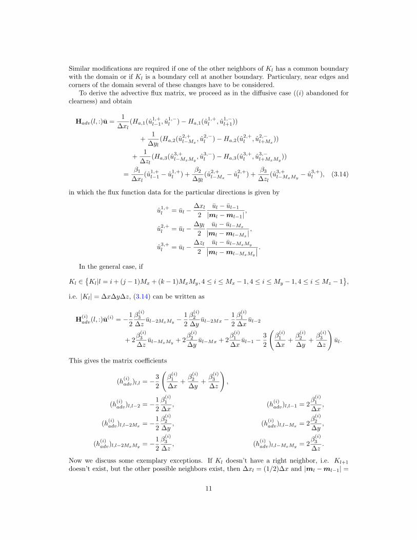
To derive the advective flux matrix, we proceed as in the diffusive case ((i) abandoned forclearness) and obtain

Hadv(l, :)u =1

∆xl(Ha,1(u1,+

l−1, u1,−l )−Ha,1(u1,+

l , u1,−l+1))

+1

∆yl(Ha,2(u2,+

l−Mx, u2,−l )−Ha,2(u2,+

l , u2,−l+Mx

))

+1

∆zl(Ha,3(u3,+

l−MxMy, u3,−l )−Ha,3(u3,+

l , u3,−l+MxMy

))

=β1

∆xl(u1,+l−1 − u

1,+l ) +

β2

∆yl(u2,+l−Mx

− u2,+l ) +

β3

∆zl(u3,+l−MxMy

− u3,+l ), (3.14)

in which the flux function data for the particular directions is given by

u1,+l = ul −

∆xl2

ul − ul−1

|ml −ml−1|,

u2,+l = ul −

∆yl2

ul − ul−Mx

|ml −ml−Mx|,

u3,+l = ul −

∆zl2

ul − ul−MxMy∣∣ml −ml−MxMy

∣∣ .In the general case, if

Kl ∈Kl|l = i+ (j − 1)Mx + (k− 1)MxMy, 4 ≤ i ≤Mx − 1, 4 ≤ i ≤My − 1, 4 ≤ i ≤Mz − 1

,

i.e. |Kl| = ∆x∆y∆z, (3.14) can be written as

H(i)adv(l, :)u

(i) = −12β

(i)3

∆zul−2MxMy

− 12β

(i)2

∆yul−2Mx −

12β

(i)1

∆xul−2

+ 2β

(i)3

∆zul−MxMy

+ 2β

(i)2

∆yul−Mx + 2

β(i)1

∆xul−1 −

32

(β

(i)1

∆x+β

(i)2

∆y+β

(i)3

∆z

)ul.

This gives the matrix coefficients

(h(i)adv)l,l = −3

2

(β

(i)1

∆x+β

(i)2

∆y+β

(i)3

∆z

),

(h(i)adv)l,l−2 = −1

2β

(i)1

∆x, (h(i)

adv)l,l−1 = 2β

(i)1

∆x,

(h(i)adv)l,l−2Mx

= −12β

(i)2

∆y, (h(i)

adv)l,l−Mx= 2

β(i)2

∆y,

(h(i)adv)l,l−2MxMy

= −12β

(i)3

∆z, (h(i)

adv)l,l−MxMy= 2

β(i)3

∆z.

Now we discuss some exemplary exceptions. If Kl doesn’t have a right neighbor, i.e. Kl+1

doesn’t exist, but the other possible neighbors exist, then ∆xl = (1/2)∆x and |ml −ml−1| =

11

(3/4)∆x, which leads to

(h(i)adv)l,l = −1

6

(16β

(i)1

∆x+ 9

β(i)2

∆y+ 9

β(i)3

∆z

),

(h(i)adv)l,l−1 =

113β

(i)1

∆x, (h(i)

adv)l,l−2 = −β(i)1

∆x,

while the remaining matrix entries are left unchanged. On the other side, if Kl−2 has a commonboundary with the domain, then |ml−1 −ml−2| = (3/4)∆x and so we have

(h(i)adv)l,l = −3

2

(β

(i)1

∆x+β

(i)2

∆y+β

(i)3

∆z

),

(h(i)adv)l,l−1 =

136β

(i)1

∆x, (h(i)

adv)l,l−2 = −23β

(i)1

∆x.

In the case that Kl−2 does not exist, since Kl−1 has a common boundary with the domain, wehave to take the boundary condition into account. As discussed above we set u1,+

l−1 = ul−1 andget

(h(i)adv)l,l = −1

6

(10β

(i)1

∆x+ 9

β(i)2

∆y+ 9

β(i)3

∆z

),

(h(i)adv)l,l−1 =

53β

(i)1

∆x, (h(i)

adv)l,l−2 = 0.

Finally, ifKl has a common boundary with the domain on the left, we have |Kl| = (1/2)∆x∆y∆zand u1,−

l = ul−1 = ul, which leads to

(h(i)adv)l,l = −3

(β

(i)2

∆y+β

(i)3

∆z

),

(h(i)adv)l,l−2 = 0, (h(i)

adv)l,l−1 = 0.

Considering these exceptional cases additionally in the y- and z-direction, completes the deriva-tion of the matrix structure.

In order to use QMR as linear solver the transpose (Jnewt)T must be available. Numericalexperiments have shown that there is no benefit from using QMR, since for instance BiCGSTABand GMRES are faster solvers which do not require matrix-vector products with the transpose.Hence, there is no benefit from an implementation of the matrix-vector product with (Jnewt)T .

III.D Parallel Implementation

The code used to perform the parallel computations presented in this paper is an extensionof the one described in [2], which uses MPI for parallel communications. Please note that theresults in this paper were computed on a newer cluster than used in [2].

In order to distribute the vector of unknowns (3.8) among P processes, we split the mesh inz-direction and distribute the unknowns accordingly. In the following, we call a submesh of sizeMxMy with only one cell in z-direction a slice. Given a mesh with Mz cells in z-direction, eachof the P parallel processes contains the data of a submesh of size MxMy(Mz/P ), i.e. Mz/Pslices of the original mesh.

To compute the matrix-vector products needed in the Krylov subspace method, communi-cation between neighboring processes is required. Denoting the portion of u which is available

12

on process 0 ≤ p < P by up = (u(p−1)MxMy(Mz/P )+1, . . . , upMxMy(Mz/P ))T , we see from Sec-tion III.C that the computation of (Hdiff u)p can be accomplished locally on process p if andonly if the first slice of up+1 and the last slice of up−1 are available besides up.

Regarding the advective matrix, Section III.C shows that the computation of (Hadvu)pneeds the last two slices of up−1, but none of up+1. Thus, one additional slice if needed fromprocess p− 1.

On interconnect networks in clusters, latency is a much more significant issue than band-width. Therefore, the cost associated with communicating two slices from process p − 1 andone slice from process p+1 in the finite volume method will not measurably change the parallelbehavior of the code, compared to one slice only from each for the finite element method. Thus,we expect parallel performance of the finite volume method to be as good as that of the finiteelement method.

IV CONVERGENCE STUDIES

Here we present convergence studies for the test cases of Section II. Particularly, we show theconvergence of the finite volume scheme, when point sources are present. In addition, we list theresults obtained by the finite element scheme from [2] whenever possible, i.e. if the advectionterm is dropped.

For both methods, the L2-norm ‖u− uh‖L2(Ω) is used. The true solution is denoted by uand uh is its numerical approximation. Classical results for the spatial error in this norm havethe form

‖u(·, t)− uh(·, t)‖L2(Ω) ≤ C hq for all 0 < t ≤ tfin, (4.1)

where the constant C is independent of the mesh size h. The number q is the convergence orderof the spatial discretization. For the finite element method, the classical theory for trilinearbasis functions specifies q = 2, see, e.g., [12]. The classical theory requires the source terms tobe in the function space L2(Ω), which is not true for the Dirac delta distribution. The heuristicarguments and computational results of [2] indicate q = 0.5 in three spatial dimensions, whichhas recently been rigorously confirmed [4]. For the finite volume method presented in theprevious section, one would expect q = 2 for smooth source terms, as well. For non-smoothsources however, there is no clear heuristic argument. It is the purpose of the following studiesto determine this order.

Here we use this strategy for the test cases with nonsmooth source terms, otherwise wecompare to the true solution.

All errors were measured in the L2-norm and the error is computed as the difference of thenumerical solution and a representation of the exact solution on a finer mesh. When usingfinite elements this representation is the trilinear nodal interpolant. In the finite volume case,we use the piecewise linear representation described in Section III.A.

In Sections IV.A and IV.B the finite element reference solution was computed on a meshwith 256 × 256 × 1024 equidistant cells and the finite volume reference on the correspondingdual mesh. Besides the errors, the following tables show the estimated convergence order, whichwas calculated using the formula

qest = log2

(‖e2h‖‖eh‖

),

in which eh denotes the error computed with respect to a numerical solution on a mesh withmaximum mesh width h. For the finite volume results the mesh size given in the tables is thesize of the primal mesh, instead of the size of the dual mesh.

To stop the BiCGSTAB iterations we choose εlin = 10−2. The parameters to control thetime step selection in the NDFk method are εoderel = 10−6 and εodeabs = 10−8 and the tolerance forthe Newton solver is εnewt = 10−4.

13

Table 4.1: L2-error on Ω against the true solution for the diffusive test problem with homoge-neous right hand side for FE and FV method.

t = 2 t = 3 t = 416× 16× 64 2.4312e–01 2.1704e–01 1.9429e–01

32× 32× 128 6.0228e–02 (2.0132) 5.3671e–02 (2.0157) 4.7955e–02 (2.0184)64× 64× 256 1.4390e–02 (2.0654) 1.2805e–02 (2.0674) 1.1416e–02 (2.0706)

128× 128× 512 2.9260e–03 (2.2981) 2.5918e–03 (2.3046) 2.2940e–03 (2.3152)(a) Finite element method

t = 2 t = 3 t = 416× 16× 64 4.1603e–01 4.0114e–01 3.8584e–01

32× 32× 128 1.0678e–01 (1.9620) 1.0243e–01 (1.9695) 9.8288e–02 (1.9729)64× 64× 256 2.6435e–02 (2.0142) 2.5353e–02 (2.0144) 2.4333e–02 (2.0141)

128× 128× 512 6.2654e–03 (2.0769) 6.0116e–03 (2.0763) 5.7763e–03 (2.0747)(b) Finite volume method

IV.A Diffusion with Homogeneous and Non-Smooth Source Term

Here we consider the unsteady scalar diffusive test problems from Section II.B.2. The errorsof both the finite element method and the finite volume method can be seen in Table 4.1(homogeneous right hand side) and Table 4.2 (point source).

With respect to the homogeneous right hand side we observe second order convergence forboth schemes, as expected by construction.

For the test problem with a point source, the convergence theory from [4] shows that sucha source term reduces the convergence order of the finite element method to q = 0.5 in threedimensions. For the finite volume method there is no such convergence theory available (atleast not to our knowledge), but we can expect the order to be equally reduced.

This is confirmed by the numerical results shown in Table 4.2. We see that for both meth-ods the convergence order is reduced from q = 2 to q = 0.5. In particular, we observe theconvergence of the finite volume scheme in the presence of point sources.

IV.B Advection-Diffusion-Reaction Equation

We now consider the advection-diffusion reaction equation with different source terms. Inparticular this equation contains an advective term. Since the finite element method from [2] isnot applicable to problems including advection, we only present results obtained with the finitevolume scheme. We consider the two different source terms, namely the smooth source termand the non-smooth source term, from Section II.B.1. The results can be found in Table 4.3.

As before in the purely diffusive test case, we observe second order convergence for thesmooth source terms, whereas the convergence order drops to 0.5 for the non-smooth sourceterm.

IV.C Pure Advection

This Section shows the errors and the convergence order for the pure advection test case fromSection II.B.3. From Table 4.4 we observe second order convergence.

In order to solve this problem with a finite element method an extra stabilization mecha-nism would need to be introduced to avoid oscillations. There is a vast amount of literatureconcerning this problem, see [5] for example, but due to the upwind flux function this is not anissue regarding the finite volume method.

14

Table 4.2: L2-error on Ω against the reference solution for the diffusive test problem withnon-smooth source term for FE and FV method.

t = 2 t = 3 t = 416× 16× 64 5.4249e+01 5.0676e+01 5.0706e+01

32× 32× 128 3.6689e+01 (0.5643) 3.7651e+01 (0.4286) 3.7806e+01 (0.4235)64× 64× 256 2.6378e+01 (0.4760) 2.6396e+01 (0.5124) 2.6400e+01 (0.5181)

128× 128× 512 1.6083e+01 (0.7138) 1.6083e+01 (0.7147) 1.6084e+01 (0.7149)(a) Finite element method

t = 2 t = 3 t = 416× 16× 64 7.6451e+01 8.5493e+01 8.8933e+01

32× 32× 128 6.4231e+01 (0.2513) 6.5344e+01 (0.3877) 6.5578e+01 (0.4395)64× 64× 256 4.6063e+01 (0.4797) 4.6135e+01 (0.5022) 4.6152e+01 (0.5068)

128× 128× 512 3.0898e+01 (0.5761) 3.0903e+01 (0.5781) 3.0905e+01 (0.5786)(b) Finite volume method

Table 4.3: Finite volume L2-error on Ω for the advection-diffusion-reaction problem with dif-ferent source terms.

t = 2 t = 3 t = 416× 16× 64 4.3545e–01 4.3988e–01 4.4475e–01

32× 32× 128 1.1677e–01 (1.8988) 1.2002e–01 (1.8738) 1.2341e–01 (1.8495)64× 64× 256 2.9780e–02 (1.9713) 3.1088e–02 (1.9489) 3.2453e–02 (1.9271)

128× 128× 512 7.2491e–03 (2.0385) 7.7004e–03 (2.0134) 8.1655e–03 (1.9907)(a) Smooth source term, error compared to true solution

t = 2 t = 3 t = 416× 16× 64 6.4421e+01 6.6058e+01 6.6523e+01

32× 32× 128 5.2605e+01 (0.2923) 5.2981e+01 (0.3183) 5.3058e+01 (0.3263)64× 64× 256 4.0491e+01 (0.3776) 4.0534e+01 (0.3863) 4.0543e+01 (0.3881)

128× 128× 512 2.8725e+01 (0.4953) 2.8728e+01 (0.4967) 2.8729e+01 (0.4969)(b) Non-smooth source term, error compared against reference solution

Table 4.4: Finite volume L2-error on Ω for the pure advection problem with homogeneoussource term.

t = 2 t = 3 t = 4128× 128× 128 1.0605e–01 1.4547e–01 1.7831e–01256× 256× 256 3.1166e–02 (1.7667) 4.5994e–02 (1.6612) 6.0303e–02 (1.5641)512× 512× 512 7.9835e–03 (1.9649) 1.1946e–02 (1.9449) 1.5895e–02 (1.9237)

1024× 1024× 1024 1.9993e–03 (1.9975) 2.9984e–03 (1.9943) 3.9971e–03 (1.9915)(a) Error compared to true solution

15

V SIMULATION OF CALCIUM WAVES

The convergence tests of the Section IV had the purpose of ensuring that the implementednumerical method is reliable and trustworthy for the application problem with point sources.This section reports one set of results for the problem of self-initiated calcium waves, whosemodel was detailed in Section II.A as motivation. Table 2.1 lists the model parameters. Recallfrom there the spatial domain Ω = (−6.4, 6.4)× (−6.4, 6.4)× (−32.0, 32.0) in units of µm and alarge final time of tfin = 1, 000 ms for long-time simulations. Simulations of this problem havetwo purposes: One is to determine if a given set of model parameters allows for self-initiationof a calcium wave. The other is to determine if self-initiation repeats, for an overall effect ofseveral waves of increasing calcium concentration. To this end, it is vital that the final time belarge enough to allow for several waves in the duration of the simulation.

The following results were obtained with the mesh size 128 × 128 × 512 using the finitevolume method. Corresponding studies on other meshes with both the finite volume and finiteelement methods, except on very coarse meshes, gave equivalent results; due to the pseudorandom number generator in the probabilistic term that determines the opening or closing ofeach calcium release unit (CRU), some variation in detail from run to run is expected.

Figures 5.1, 5.2, and 5.3 each show snapshots of time-dependent simulations at ten pointsin time. Figure 5.1 plots open calcium release units throughout the cell, each marked by a fatdot (the size of the dot does not have meaning). The simulation starts with no open CRUsat t = 0 ms. By time t = 100 ms, a few CRUs are open, as shown in the first sub-plot ofFigure 5.1. They form a small cluster, as far as visible from this plot (but see Figure 5.3below), which is consistent with the mechanism modeled: Once a CRU happens to open andit injects calcium into the cell, diffusion carries the calcium to its neighboring CRUs, whoseprobability for opening increasing with the increasing calcium concentration. This is how entirewaves can self-initiate, which is born out by the second sub-plot for t = 200 ms, in which theoriginal wave has traveled in both directions through the cell. Moreover, we can see that anew wave is about to initiate at approximately the same location as the one for t = 100 ms.The following sub-plots in Figure 5.1 bear out the repeated self-initiation and travel of wavesthrough the cell. This confirms that the model is behaving correctly and the parameters inTable 2.1 are meaningful. Recall that there is a lattice of 15 × 15 × 31 CRUs throughout theinterior of the cell. Of these 6,975 CRUs, on the order of hundreds are typically open at anygiven point in time.

Figure 5.2 presents isosurface plots of the calcium concentration at the same ten points intime. The critical value used in these plots is 65 µM, which is above the rest value of 0.1 µMand safely below the maximum value of several hundreds reached at an open CRU location. Itis expected that the calcium concentration is high (above the critical value) around open CRUs.But what is also crucial to determine by this simulation is that the calcium concentration returnto its rest value after a wave has passed and in between waves. This is clearly born out by thesub-plots at latter points in time. Notice that long-time simulations are necessary to confirmthis fact; a short study up to, say, 200 ms can by contrast only confirm the self-initiation of awave, not that the concentration returns to rest values repeatedly.

Figure 5.3 depicts confocal images of the simulation results at the ten points in time, whichshow the calcium concentration in a two-dimensional x-z-cross-section of the domain at theplane y = 0. These images are designed to emulate the appearance of experimental results.They can provide additional detailed understanding of the shape of a wave. Recall that inFigure 5.1 at t = 100 ms, one can only make out a cluster of open CRUs, and at t = 200 ms,Figures 5.1 and 5.2 essentially show two blobs without discernable shape. By contrast, the sub-plots in Figure 5.3 present the shape of the CRU waves as spirals (top and bottom of domaincut off a portion). This confirms experimentally observed results and demonstrates that oursimulator can reproduce this effect.

16

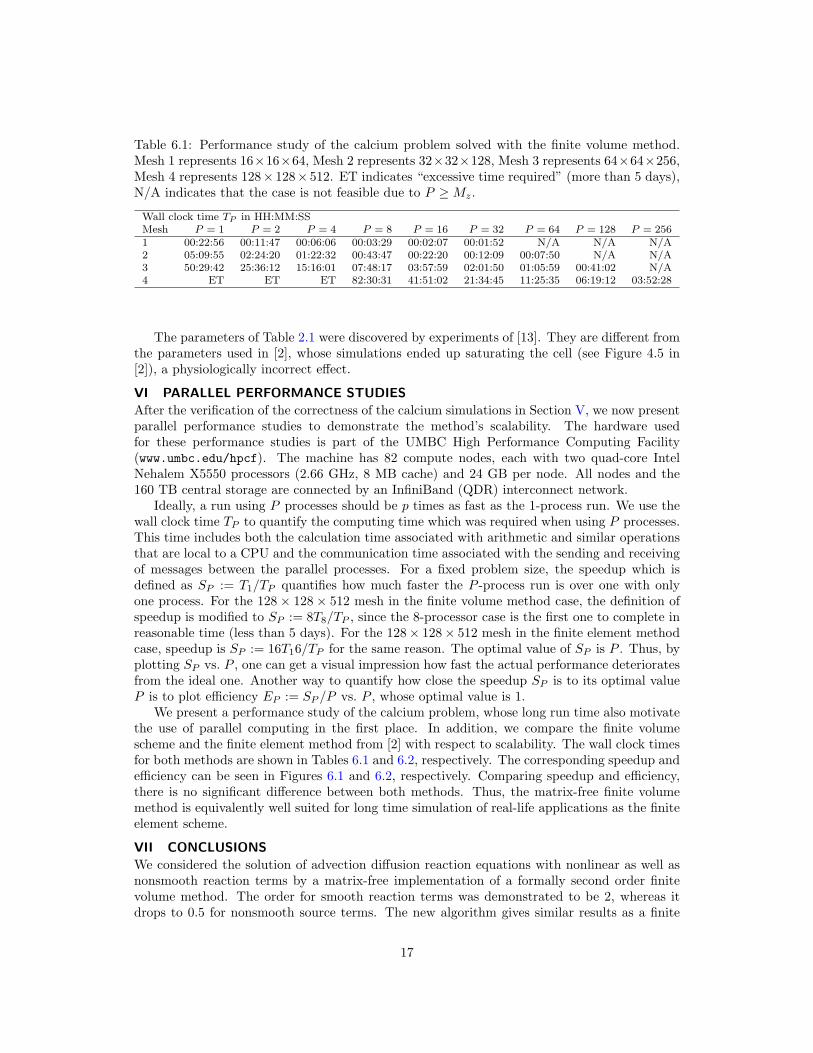
Table 6.1: Performance study of the calcium problem solved with the finite volume method.Mesh 1 represents 16×16×64, Mesh 2 represents 32×32×128, Mesh 3 represents 64×64×256,Mesh 4 represents 128× 128× 512. ET indicates “excessive time required” (more than 5 days),N/A indicates that the case is not feasible due to P ≥Mz.

Wall clock time TP in HH:MM:SSMesh P = 1 P = 2 P = 4 P = 8 P = 16 P = 32 P = 64 P = 128 P = 2561 00:22:56 00:11:47 00:06:06 00:03:29 00:02:07 00:01:52 N/A N/A N/A2 05:09:55 02:24:20 01:22:32 00:43:47 00:22:20 00:12:09 00:07:50 N/A N/A3 50:29:42 25:36:12 15:16:01 07:48:17 03:57:59 02:01:50 01:05:59 00:41:02 N/A4 ET ET ET 82:30:31 41:51:02 21:34:45 11:25:35 06:19:12 03:52:28

The parameters of Table 2.1 were discovered by experiments of [13]. They are different fromthe parameters used in [2], whose simulations ended up saturating the cell (see Figure 4.5 in[2]), a physiologically incorrect effect.

VI PARALLEL PERFORMANCE STUDIES

After the verification of the correctness of the calcium simulations in Section V, we now presentparallel performance studies to demonstrate the method’s scalability. The hardware usedfor these performance studies is part of the UMBC High Performance Computing Facility(www.umbc.edu/hpcf). The machine has 82 compute nodes, each with two quad-core IntelNehalem X5550 processors (2.66 GHz, 8 MB cache) and 24 GB per node. All nodes and the160 TB central storage are connected by an InfiniBand (QDR) interconnect network.

Ideally, a run using P processes should be p times as fast as the 1-process run. We use thewall clock time TP to quantify the computing time which was required when using P processes.This time includes both the calculation time associated with arithmetic and similar operationsthat are local to a CPU and the communication time associated with the sending and receivingof messages between the parallel processes. For a fixed problem size, the speedup which isdefined as SP := T1/TP quantifies how much faster the P -process run is over one with onlyone process. For the 128× 128× 512 mesh in the finite volume method case, the definition ofspeedup is modified to SP := 8T8/TP , since the 8-processor case is the first one to complete inreasonable time (less than 5 days). For the 128× 128× 512 mesh in the finite element methodcase, speedup is SP := 16T16/TP for the same reason. The optimal value of SP is P . Thus, byplotting SP vs. P , one can get a visual impression how fast the actual performance deterioratesfrom the ideal one. Another way to quantify how close the speedup SP is to its optimal valueP is to plot efficiency EP := SP /P vs. P , whose optimal value is 1.

We present a performance study of the calcium problem, whose long run time also motivatethe use of parallel computing in the first place. In addition, we compare the finite volumescheme and the finite element method from [2] with respect to scalability. The wall clock timesfor both methods are shown in Tables 6.1 and 6.2, respectively. The corresponding speedup andefficiency can be seen in Figures 6.1 and 6.2, respectively. Comparing speedup and efficiency,there is no significant difference between both methods. Thus, the matrix-free finite volumemethod is equivalently well suited for long time simulation of real-life applications as the finiteelement scheme.

VII CONCLUSIONS

We considered the solution of advection diffusion reaction equations with nonlinear as well asnonsmooth reaction terms by a matrix-free implementation of a formally second order finitevolume method. The order for smooth reaction terms was demonstrated to be 2, whereas itdrops to 0.5 for nonsmooth source terms. The new algorithm gives similar results as a finite

17

t = 100 t = 200

t = 300 t = 400

t = 500 t = 600

t = 700 t = 800

t = 900 t = 1,000

Figure 5.1: Open calcium release units throughout the cell using finite volume method withmesh size 128× 128× 512.

18

t = 100 t = 200

t = 300 t = 400

t = 500 t = 600

t = 700 t = 800

t = 900 t = 1,000

Figure 5.2: Isosurface plots of the calcium concentration using finite volume method with meshsize 128× 128× 512.

19

t = 100 t = 200

t = 300 t = 400

t = 500 t = 600

t = 700 t = 800

t = 900 t = 1,000

Figure 5.3: Confocal image plots of the calcium concentration using finite volume method withmesh size 128× 128× 512.

20

(a) Observed speedup SP (b) Observed efficiency EP

Figure 6.1: Performance study of the calcium problem solved with finite volume method.

Table 6.2: Performance study of the calcium problem solved with the finite element method.Mesh 1 represents 16×16×64, Mesh 2 represents 32×32×128, Mesh 3 represents 64×64×256,Mesh 4 represents 128× 128× 512. ET indicates “excessive time required” (more than 5 days),N/A indicates that the case is not feasible due to P > Mz.

Wall clock time TP in HH:MM:SSMesh P = 1 P = 2 P = 4 P = 8 P = 16 P = 32 P = 64 P = 128 P = 2561 00:08:41 00:04:37 00:02:13 00:01:20 00:00:46 00:00:31 00:00:24 N/A N/A2 09:23:19 04:43:52 02:33:54 01:19:35 00:40:40 00:21:53 00:12:57 00:08:45 N/A3 67:04:28 32:09:20 18:10:07 09:17:32 04:42:50 02:25:47 01:19:28 00:45:09 00:29:064 ET ET ET ET 74:11:02 38:00:33 19:57:57 10:49:08 06:16:11

element scheme considered in previous articles but can handle advection dominated problems.Finally, strong parallel scaling for up to 256 processes was demonstrated.

(a) Observed speedup SP (b) Observed efficiency EP

Figure 6.2: Performance study of the calcium problem solved with finite element method.

21

ACKNOWLEDGMENTS

Xuan Huang acknowledges support from the UMBC High Performance Computing Facility(HPCF). The hardware used in the computational studies is part of HPCF. The facility is sup-ported by the U.S. National Science Foundation through the MRI program (grant nos. CNS–0821258 and CNS–1228778) and the SCREMS program (grant no. DMS–0821311), with addi-tional substantial support from the University of Maryland, Baltimore County (UMBC). Seewww.umbc.edu/hpcf for more information on HPCF and the projects using its resources. Fur-thermore, the work of the authors Birken, Gobbert and Meister was supported by the GermanResearch Foundation as part of the SFB/TRR TR 30, project C2.

References

[1] D. A. Knoll, D. E. Keyes, Jacobian-free Newton-Krylov methods: a survey of approachesand applications, J. Comput. Phys. 193 (2004) 357–397.

[2] M. K. Gobbert, Long-time simulations on high resolution meshes to model calcium wavesin a heart cell, SIAM J. Sci. Comput. 30 (6) (2008) 2922–2947.

[3] A. L. Hanhart, M. K. Gobbert, L. T. Izu, A memory-efficient finite element method forsystems of reaction-diffusion equations with non-smooth forcing, J. Comput. Appl. Math.169 (2) (2004) 431–458.

[4] T. I. Seidman, M. K. Gobbert, D. W. Trott, M. Kruzık, Finite element approximationfor time-dependent diffusion with measure-valued source, Numer. Math. 122 (4) (2012)709–723.

[5] H.-G. Roos, M. Stynes, L. Tobiska, Robust Numerical Methods for Singularly PerturbedDifferential Equations, 2nd Edition, Vol. 24 of Springer Series in Computational Mathe-matics, Springer-Verlag, 2008.

[6] J. Santos, P. de Oliveira, A converging finite volume scheme for hyperbolic conservationlaws with source terms, J. Comput. Appl. Math. 111 (1-2) (1999) 239–251.

[7] Y. Yang, C.-W. Shu, Discontinuous galerkin method for hyperbolic equations involvingδ-singularities: negative-order norm error estimates and applications, Numerische Mathe-matik (2013) 1–29.URL http://dx.doi.org/10.1007/s00211-013-0526-8

[8] C.-W. Shu, High order weighted essentially nonoscillatory schemes for convection domi-nated problems, SIAM Rev. 51 (1) (2009) 82–126.

[9] L. F. Shampine, M. W. Reichelt, The MATLAB ODE suite, SIAM J. Sci. Comput. 18 (1)(1997) 1–22.

[10] L. F. Shampine, Numerical Solution of Ordinary Differential Equations, Chapman & Hall,1994.

[11] Y. Saad, Iterative Methods for Sparse Linear Systems, 2nd Edition, SIAM, 2003.

[12] V. Thomee, Galerkin Finite Element Methods for Parabolic Problems, 2nd Edition, Vol. 25of Springer Series in Computational Mathematics, Springer-Verlag, 2006.

[13] Z. A. Coulibaly, B. E. Peercy, M. K. Gobbert, Spontaneous spiral wave initiation in a 3-Dcardiac cell, in preparation.

22