lecture 12: advection and diffusion in environmental flows · lecture 12: advection and diffusion...

OCEN 678 Fluid Dynamics for Ocean and Environmental Engineering

S. Socolofsky 1

Lecture 12: Advection and Diffusion in Environmental Flows

Learning Objectives:

1. List and apply the basic assumptions used in classical fluid dynamics for ocean

engineering

2. Identify and formulate the physical interpretation of the mathematical terms in solutions

to fluid dynamics problems

Topics/Outline:

1. Solution for an instantaneous point source

2. Distributed source solutions

3. Examples

Reading:

Socolofsky, S.A. and Jirka, G.H. (2004). Special Topics on Mixing and Transport Processes

in the Environment.

Chapter 2: Advection-diffusion equation. Available on-line from:

https://ceprofs.civil.tamu.edu/ssocolofsky/OCENx89/book.html

2. Advective Diffusion Equation

In nature, transport occurs in fluids through the combination of advection and diffusion. The

previous chapter introduced diffusion and derived solutions to predict diffusive transport in

stagnant ambient conditions. This chapter incorporates advection into our diffusion equation

(deriving the advective diffusion equation) and presents various methods to solve the resulting

partial differential equation for different geometries and contaminant conditions.

2.1 Derivation of the advective diffusion equation

Before we derive the advective diffusion equation, we look at a heuristic description of the effect

of advection. To conceptualize advection, consider our pipe problem from the previous chapter.

Without pipe flow, the injected tracer spreads equally in both directions, describing a Gaussian

distribution over time. If we open a valve and allow water to flow in the pipe, we expect the

center of mass of the tracer cloud to move with the mean flow velocity in the pipe. If we move

our frame of reference with that mean velocity and assume the inviscid case, then we expect the

solution to look the same as before. This new reference frame is

η = x − (x0 + ut) (2.1)

where η is the moving reference frame spatial coordinate, x0 is the injection point of the tracer,

u is the mean flow velocity, and ut is the distance traveled by the center of mass of the cloud

in time t. If we substitute η for x in our solution for a point source in stagnant conditions we

obtain

C(x, t) =M

A√

4πDtexp

(

−(x − (x0 + ut))2

4Dt

)

. (2.2)

To test whether this solution is correct, we need to derive a general equation for advective

diffusion and compare its solution to this one.

2.1.1 The governing equation

The derivation of the advective diffusion equation relies on the principle of superposition: ad-

vection and diffusion can be added together if they are linearly independent. How do we know

if advection and diffusion are independent processes? The only way that they can be dependent

is if one process feeds back on the other. From the previous chapter, diffusion was shown to be

a random process due to molecular motion. Due to diffusion, each molecule in time δt will move

Copyright c© 2004 by Scott A. Socolofsky and Gerhard H. Jirka. All rights reserved.

30 2. Advective Diffusion Equation

Jx,in Jx,out

x

-y

z

δxδy

δz

u

Fig. 2.1. Schematic of a control volume with crossflow.

either one step to the left or one step to the right (i.e. ±δx). Due to advection, each molecule

will also move uδt in the cross-flow direction. These processes are clearly additive and indepen-

dent; the presence of the crossflow does not bias the probability that the molecule will take a

diffusive step to the right or the left, it just adds something to that step. The net movement of

the molecule is uδt ± δx, and thus, the total flux in the x-direction Jx, including the advective

transport and a Fickian diffusion term, must be

Jx = uC + qx

= uC − D∂C

∂x. (2.3)

We leave it as an exercise for the reader to prove that uC is the correct form of the advective

term (hint: consider the dimensions of qx and uC).

As we did in the previous chapter, we now use this flux law and the conservation of mass

to derive the advective diffusion equation. Consider our control volume from before, but now

including a crossflow velocity, u = (u, v, w), as shown in Figure 2.1. Here, we follow the derivation

in Fischer et al. (1979). From the conservation of mass, the net flux through the control volume

is

∂M

∂t=∑

min −∑

mout, (2.4)

and for the x-direction, we have

δm|x =

(

uC − D∂C

∂x

)∣

∣

∣

∣

1δyδz −

(

uC − D∂C

∂x

)∣

∣

∣

∣

2δyδz. (2.5)

As before, we use linear Taylor series expansion to combine the two flux terms, giving

uC|1 − uC|2 = uC|1 −(

uC|1 +∂(uC)

∂x

∣

∣

∣

∣

1δx

)

= −∂(uC)

∂xδx (2.6)

2.1 Derivation of the advective diffusion equation 31

and

− D∂C

∂x

∣

∣

∣

∣

1+ D

∂C

∂x

∣

∣

∣

∣

2= −D

∂C

∂x

∣

∣

∣

∣

1+

(

D∂C

∂x

∣

∣

∣

∣

1+

∂

∂x

(

D∂C

∂x

)∣

∣

∣

∣

1δx

)

= D∂2C

∂x2δx. (2.7)

Thus, for the x-direction

δm|x = −∂(uC)

∂xδxδyδz + D

∂2C

∂x2δxδyδz. (2.8)

The y- and z-directions are similar, but with v and w for the velocity components, giving

δm|y = −∂(vC)

∂yδyδxδz + D

∂2C

∂y2δyδxδz (2.9)

δm|z = −∂(wC)

∂zδzδxδy + D

∂2C

∂z2δzδxδy. (2.10)

Substituting these results into (2.4) and recalling that M = Cδxδyδz, we obtain

∂C

∂t+ ∇ · (uC) = D∇2C (2.11)

or in Einsteinian notation

∂C

∂t+

∂uiC

∂xi= D

∂2C

∂x2i

, (2.12)

which is the desired advective diffusion (AD) equation. We will use this equation extensively in

the remainder of this text.

Note that these equations implicitly assume that D is constant. When considering a variable

D, the right-hand-side of (2.12) has the form

∂

∂xi

(

Dij∂C

∂xj

)

. (2.13)

2.1.2 Point-source solution

To check whether our initial suggestion (2.2) for a solution to (2.12) was correct, we substitute

the coordinate transformation for the moving reference frame into the one-dimensional version

of (2.12). In the one-dimensional case, u = (u, 0, 0), and there are no concentration gradients in

the y- or z-directions, leaving us with

∂C

∂t+

∂(uC)

∂x= D

∂2C

∂x2. (2.14)

Our coordinate transformation for the moving system is

η = x − (x0 + ut) (2.15)

τ = t, (2.16)

and this can be substituted into (2.14) using the chain rule as follows


0 1 2 3 4 5 6 7 8 9 100

0.5

1

1.5Solution of the advective−diffusion equation

Position

Con

cent

ratio

n

t1

t2 t

3

Cmax

Fig. 2.2. Schematic solution of the advective diffusion equation in one dimension. The dotted line plots themaximum concentration as the cloud moves downstream.

∂C

∂τ

∂τ

∂t+

∂C

∂η

∂η

∂t+ u

(

∂C

∂η

∂η

∂x+

∂C

∂τ

∂τ

∂x

)

=

D

(

∂

∂η

∂η

∂x+

∂

∂τ

∂τ

∂x

)(

∂C

∂η

∂η

∂x+

∂C

∂τ

∂τ

∂x

)

(2.17)

which reduces to

∂C

∂τ= D

∂2C

∂η2. (2.18)

This is just the one-dimensional diffusion equation (1.29) in the coordinates η and τ with solution

for an instantaneous point source of

C(η, τ) =M

A√

4πDτexp

(

− η2

4Dτ

)

. (2.19)

Converting the solution back to x and t coordinates (by substituting (2.15) and (2.16)), we

obtain (2.2); thus, our intuitive guess for the superposition solution was correct. Figure 2.2

shows the schematic behavior of this solution for three different times, t1, t2, and t3.

2.1.3 Incompressible fluid

For an incompressible fluid, (2.12) can be simplified by using the conservation of mass equation

for the ambient fluid. In an incompressible fluid, the density is a constant ρ0 everywhere, and

the conservation of mass equation reduces to the continuity equation

∇ · u = 0 (2.20)

(see, for example Batchelor (1967)). If we expand the advective term in (2.12), we can write

∇ · (uC) = (∇ · u)C + u · ∇C. (2.21)

by virtue of the continuity equation (2.20) we can take the term (∇·u)C = 0; thus, the advective

diffusion equation for an incompressible fluid is

2.1 Derivation of the advective diffusion equation 33

∂C

∂t+ ui

∂C

∂xi= D

∂2C

∂x2i

. (2.22)

This is the form of the advective diffusion equation that we will use the most in this class.

2.1.4 Rules of thumb

We pause here to make some observations regarding the AD equation and its solutions.

First, the solution in Figure 2.2 shows an example where the diffusive and advective transport

are about equally important. If the crossflow were stronger (larger u), the cloud would have less

time to spread out and would be narrower at each ti. Conversely, if the diffusion were faster

(larger D), the cloud would spread out more between the different ti and the profiles would

overlap. Thus, we see that diffusion versus advection dominance is a function of t, D, and u,

and we express this property through the non-dimensional Peclet number

Pe =D

u2t, (2.23)

or for a given downstream location L = ut,

Pe =D

uL. (2.24)

For Pe � 1, diffusion is dominant and the cloud spreads out faster than it moves downstream;

for Pe � 1, advection is dominant and the cloud moves downstream faster than it spreads out.

It is important to note that the Peclet number is dependent on our zone of interest: for “large”

times or distances, the Peclet number is small and advection dominates.

Second, the maximum concentration decreases in the downstream direction due to diffusion.

Figure 2.2 also plots the maximum concentration of the cloud as it moves downstream. This is

obtained when the exponential term in (2.2) is 1.0. For the one-dimensional case, the maximum

concentration decreases as

Cmax(t) ∝ 1√t. (2.25)

In the two- and three-dimensional cases, the relationship is

Cmax(t) ∝ 1

tand (2.26)

Cmax(t) ∝ 1

t√

t, (2.27)

respectively.

Third, the diffusive and advective scales can be used to simplify the equations and make ap-

proximations. One of the most common questions in engineering is: when does a given equation

or approximation apply? In contaminant transport, this question is usually answered by com-

paring characteristic advection and diffusion length and time scales to the length and time scales

in the problem. For advection (subscript a) and for diffusion (subscript d), the characteristic

scales are


La = ut ; ta =L

u(2.28)

Ld =√

Dt ; td =L2

D. (2.29)

These scales can be used as a rule-of-thumb estimate for when or where certain events take

place. For instance, for a point source released in the middle of a region of width L and bounded

at ±L/2 by impermiable boundaries, the time required before the cloud can be considered well-

mixed over the region by diffusion is tm,d = L2/(8D). The coefficient value 8 is derived by

requiring that the concentration at ±L/2 be at least 97% of the maximum concentration Cmax.

These characteristic scales (easily derivable through dimensional analysis) should be memorized

and used extensively to get a rough solution to transport problems.

2.2 Solutions to the advective diffusion equation

In the previous chapter we presented a detailed solution for an instantaneous point source in a

stagnant ambient. In nature, initial and boundary conditions can be much different from that

idealized case, and this section presents a few techniques to deal with other general cases. Just as

advection and diffusion are additive, we will also show that superpostion can be used to build up

solutions to complex geometries or initial conditions from a base set of a few general solutions.

The solutions in this section parallel a similar section in Fischer et al. (1979). Appendix B

presents analytical solutions for other initial and boundary conditions, primarily obtained by

extending the techniques discussed in this section. Taken together, these solutions can be applied

to a wide range of problems.

2.2.1 Initial spatial concentration distribution

A good example of the power of superposition is the solution for an initial spatial concentration

distribution. Since advection can always be included by changing the frame of reference, we will

consider the one-dimensional stagnant case. Thus, the governing equation is

∂C

∂t= D

∂2C

∂x2. (2.30)

We will consider the homogeneous initial distribution, given by

C(x, t0) =

{

C0 if x ≤ 0

0 if x > 0(2.31)

where t0 = 0 and C0 is the uniform initial concentration, as depicted in Figure 2.3. At a point

x = ξ < 0 there is an infinitesimal mass dM = C0Adξ, where A is the cross-sectional area δyδz.

For t > 0, the concentration at any point x is due to the diffusion of mass from all the differential

elements dM . The contribution dC for a single element dM is just the solution of (2.30) for an

instantaneous point source

dC(x, t) =dM

A√

4πDtexp

(

−(x − ξ)2

4Dt

)

, (2.32)

2.2 Solutions to the advective diffusion equation 35

C

x

dM = C0Ad

C0

d x

ξ

ξFig. 2.3. Schematic of an instantaneous initial concentration distribution showing the differential element dM atthe point −ξ.

and by virtue of superposition, we can sum up all the contributions dM to obtain

C(x, t) =

∫ 0

−∞

C0dξ√4πDt

exp

(

−(x − ξ)2

4Dt

)

(2.33)

which is the superposition solution to our problem. To compute the integral, we must, as usual,

make a change of variables. The new variable ζ is defined as follows

ζ =x − ξ√

4Dt(2.34)

dζ = − dξ√4Dt

. (2.35)

Substituting ζ into the integral solution gives

C(x, t) =C0√

π

∫ x/√

4Dt

∞− exp(−ζ2)dζ. (2.36)

Note that to obtain the upper bound on the integral we set ξ = 0 in the definition for ζ given

in (2.34). Rearranging the integral gives

C(x, t) =C0√

π

∫ ∞

x/√

4Dtexp(−ζ2)dζ (2.37)

=C0√

π

[

∫ ∞

0exp(−ζ2)dζ −

∫ x/√

4Dt

0exp(−ζ2)dζ

]

. (2.38)

The first of the two integrals can be solved analytically—from a table of integrals, its solution

is√

π/2. The second integral is the so called error function, defined as

erf(ϕ) =2√π

∫ ϕ

0exp(−ζ2)dζ. (2.39)

Solutions to the error function are generally found in tables or as built-in functions in a spread-

sheet or computer programming language. Hence, our solution can be written as

C(x, t) =C0

2

(

1 − erf

(

x√4Dt

))

. (2.40)

Figure 2.4 plots this solution for C0 = 1 and for increasing times t.


−5 −4 −3 −2 −1 0 1 2 3 4 50

0.2

0.4

0.6

0.8

1Solution for instantaneous step function for x < 0

Position

Con

cent

ratio

n

Increasing t

Fig. 2.4. Solution (2.40) for an instantaneous initial concentration distribution given by (2.31) with C0 = 1.

Example Box 2.1:Diffusion of an intravenous injection.

A doctor administers an intravenous injection ofan allergy fighting medicine to a patient sufferingfrom an allergic reaction. The injection takes a to-tal time T . The blood in the vein flows with meanvelocity u, such that blood over a region of lengthL = uT contains the injected chemical; the concen-tration of chemical in the blood is C0 (refer to thefollowing sketch).

L

-x x

x = 0

What is the distribution of chemical in the vein whenit reaches the heart 75 s later?

This problem is an initial spatial concentrationdistribution, like the one in Section 2.2.1. Take thepoint x = 0 at the middle of the distribution andlet the coordinate system move with the mean bloodflow velocity u. Thus, we have the initial concentra-tion distribution

C(x, t0) =

{

C0 if −L/2 < x < L/20 otherwise

where t0 = 0 at the time T/2.Following the solution method in Section 2.2.1,

the superposition solution is

C(x, t) =

∫ L/2

−L/2

C0dξ√4πDt

exp

(

− (x − ξ)2

4Dt

)

which can be expanded to give

C(x, t) =C0√4πDt

·[∫ L/2

−∞

exp

(

− (x − ξ)2

4Dt

)

dξ −∫

−L/2

−∞

exp

(

− (x − ξ)2

4Dt

)

dξ

]

.

After substituting the coordinate transformation in(2.34) and simplifying, the solution is found to be

C(x, t) =C0

2

(

erf

(

x + L/2√4Dt

)

−

erf

(

x − L/2√4Dt

))

.

Substituting t = 75 s gives the concentration distri-bution when the slug of medicine reaches the heart.

2.2.2 Fixed concentration

Another common situation is a fixed concentration at some point x1. This could be, for example,

the oxygen concentration at the air-water interface. The parameters governing the solution are

the fixed concentration C0, the diffusion coefficient D, and the coordinates (x − x0), and t.

Again, we will neglect advection since we can include it through a change of variables, and we

2.2 Solutions to the advective diffusion equation 37

0 0.5 1 1.5 2 2.5 3 3.5 4 4.5 50

0.2

0.4

0.6

0.8

1Solution for fixed concentration at x = 0

Position

Con

cent

ratio

n

Increasing t

Fig. 2.5. Solution (2.43) for a fixed concentration at x = 0 of C0 = 1.

will take x0 = 0 for simplicity. As we did for a point source, we form a similarity solution from

the governing variables, which gives us the solution form

C(x, t) = C0f

(

x√Dt

)

. (2.41)

If we define the similarity variable η = x/√

Dt and substitute it into (2.30) we obtain, as

expected, an ordinary differential equation in f and η, given by

d2f

dη2+

η

2

df

dη= 0 (2.42)

with boundary conditions f(0) = 1 and f(∞) = 0. Unfortunately, our ordinary differential

equation is non-linear. A quick look at Figure 2.4, however, might help us guess a solution. The

point at x = 0 has a fixed concentration of C0/2. If we substitute C0 as the leading coefficient

in (2.40) (instead of C0/2), maybe that would be the solution. Substitution into the differential

equation (2.42) and its boundary conditions proves, indeed, that the solution is correct, namely

C(x, t) = C0

(

1 − erf

(

x√4Dt

))

(2.43)

is the solution we seek. Figure 2.5 plots this solution for C0 = 1. Important note: this solution

is only valid for x > x0.

2.2.3 Fixed, no-flux boundaries

The final situation we examine in this section is how to incorporate no-flux boundaries. No-flux

boundaries are any surface that is impermeable to the contaminant of interest. The discussion

in this section assumes that no chemical reactions occur at the surface and that the surface is

completely impermeable.

As you might expect, we first need to find a way to specify a no-flux boundary as a boundary

condition to the governing differential equation. This is done easily using Fick’s law. Since no-

flux means that q = 0 (and taking D as constant), the boundary conditions can be expressed


Example Box 2.2:Dissolving sugar in coffee.

On a cold winter’s day you pour a cup of coffee andadd 2 g of sugar evenly distributed over the bottomof the coffee cup. The diameter of the cup is 5 cm;its height is 7 cm. If you do not stir the coffee, whendoes the concentration boundary layer first reach thetop of the cup and when does all of the sugar dis-solve? How would these answers change if you stirthe coffee?

The concentration of sugar is fixed at the satu-ration concentration at the bottom of the cup andis initially zero everywhere else. These are the sameconditions as for the fixed concentration solution;thus, the sugar distribution at height z above thebottom of the cup is

C(z, t) = C0

(

1 − erf

(

z√4Dt

))

.

The characteristic height of the concentrationboundary layer is proportional to σ =

√2Dt. As-

sume the concentration boundary layer first reachesthe top of the cup when 2σ = h = 7 cm. Solving fortime gives

tmix,bl =h2

8D.

For an order-of-magnitude estimate, take D ∼10−9 m2/s, giving

tmix,bl ≈ 6 · 105 s.

To determine how long it takes for the sugar todissolve, we must compute the mass flux of sugar atz = 0. We already computed the derivative of theerror function in Example Box 1.1. The mass flux ofsugar at z = 0 is then

m(0, t) =ADCsat√

πDt

where A is the cross-sectional area of the cup. The to-tal amount of dissolved sugar Md is the time-integralof the mass flux

Md =

∫ t

0

ADCsat√πDτ

dτ

Integrating and solving for time gives

td =M2

d π

4A2DC2sat

where td is the time it takes for the mass Md todissolve. This expression is only valid for t < tmix,bl;for times beyond tmix,bl, we must account for theboundary at the top of the cup. Assuming Csat =0.58 g/cm3, the time needed to dissolve all the sugaris

td = 5 · 104 s.

By stirring, we effectively increase the value of D.Since D is in the denominator of each of these timeestimates, we shorten the time for the sugar to dis-solve and mix throughout the cup.

as

q|Sb· n = 0

(

∂C

∂x,∂C

∂y,∂C

∂z

)∣

∣

∣

∣

Sb

· n = 0 (2.44)

where Sb is the function describing the boundary surface (i.e. Sb = f(x, y)) and n is the unit vec-

tor normal to the no-flux boundary. In the one-dimensional case, the no-flux boundary condition

reduces to

∂C

∂x

∣

∣

∣

∣

xb

= 0, (2.45)

where xb is the boundary location. This property is very helpful in interpreting concentration

measurements to determine whether a boundary, for instance, the lake bottom, is impermeable

or not.

To find a solution to a bounded problem, consider an instantaneous point source injected

at x0 with a no-flux boundary a distance L to the right as shown in Figure 2.6. Our standard

solution allows mass to diffuse beyond the no-flux boundary (as indicated by the dashed line in

2.3 Application: Diffusion in a Lake 39

Boundary

Imagesource

Realsource

Superpositionsolution

2L

C

x

x0

Fig. 2.6. Schematic of a no-flux boundary with real instantaneous point source to the left and an imaginarysource to the right. The dotted lines indicate the individual contributions from the two sources; the solid lineindicates the superposition solution.

the figure). To replace this lost mass, an image source (imaginary source) is placed to the right

of the boundary, such that it leaks the same amount of mass back to left of the boundary as

our standard solution leaked to the right. Superposing (adding) these two solutions gives us the

desired no-flux behavior at the wall. The image source is placed L to the right of the boundary,

and the solution is

C(x, t) =M

A√

4πDt

(

exp

(

−(x − x0)2

4Dt

)

+ exp

(

−(x − xi)2

4Dt

))

(2.46)

where xi = x0 + 2L. Naturally, the solution given here is only valid to the left of the boundary.

To the right of the boundary, the concentration is everywhere zero. Compute the concentration

gradient ∂C/∂x at x = 0 to prove to yourself that the no-flux boundary condition is satisfied.

The method of images becomes more complicated when multiple boundaries are concerned.

This is because the mass diffusing from the image source on the right eventually will penetrate a

boundary on the left and need its own image source. In general, when there are two boundaries,

an infinite number of image sources is required. In practice, the solution usually converges after

only a few image sources have been included (Fischer et al. 1979). For the case of an instantaneous

point source at the origin with boundaries at ±L, Fischer et al. (1979) give the image source

solution

C(x, t) =M

A√

4πDt

∞∑

n=−∞exp

(

−(x + 2nL)2

4Dt

)

. (2.47)

Obviously, the number of image sources required for the solution to converge depends on the

time scale over which the solution is to be valid. These techniques will become more clear in the

following examples and remaining chapters.

2.3 Application: Diffusion in a Lake

We return here to the application of arsenic contamination in a small lake presented in Chapter 1

(adapted from Nepf (1995)). After further investigation, it is determined that a freshwater spring

flows into the bottom of the lake with a flow rate of 10 l/s.


Example Box 2.3:Boundaries in a coffee cup.

In the previous example box we said that we haveto account for the free surface boundary when theconcentration boundary layer reaches the top of thecoffee cup. Describe the image source needed to ac-count for the free surface and state the image-sourcesolution for the concentration distribution.

We can ignore the boundaries at the sides of thecup because sugar is evenly distributed on the bot-tom of the cup. This even distribution results in∂C/∂x = ∂C/∂y = 0, which results in no net dif-fusive flux toward the cup walls.

To account for the free surface, though, we mustadd an image source with a fixed concentration ofCsat somewhere above the cup. Taking z = 0 at thebottom of the cup, the image source must be placedat z = 2h, where h is the depth of coffee in the cup.

Taking care that C(z,∞) → Csat, the superposi-tion solution for the sugar concentration distributioncan be found to be

C(z, t) = Csat

(

1 + erf

(

2h√4Dt

)

−

erf

(

z√4Dt

)

− erf

(

2h − z√4Dt

))

.

Advection. Advection is due to the flow of spring water through the lake. Assuming the spring

is not buoyant, it will spread out over the bottom of the lake and rise with a uniform vertical

flux velocity (recall that z is positive downward, so the flow is in the minus z-direction)

va = −Q/A

= −5 · 10−7 m/s. (2.48)

The concentration of arsenic at the thermocline is 8 µg/l, which results in an advective flux of

arsenic

qa = Cva

= −4 · 10−3 µg/(m2s). (2.49)

Thus, advection caused by the spring results in a vertical advective flux of arsenic through the

thermocline.

Discussion. Taking the turbulent and advective fluxes of arsenic together, the net vertical flux

of arsenic through the thermocline is

Jz = −4.00 · 10−3 + 2.93 · 10−3

= −1.10 · 10−3 µg/(m2s) (2.50)

where the minus sign indicates the net flux is upward. Thus, although the net diffusive flux is

downward, the advection caused by the stream results in the net flux at the thermocline being

upward. We can conclude that the arsenic source is likely at the bottom of the lake. The water

above the thermocline will continue to increase in concentration until the diffusive flux at the

thermocline becomes large enough to balance the advective flux through the lake, at which time

the system will reach a steady state.

2.4 Application: Fishery intake protection 41

Fisheryintake

Dam (A = 3000 m2)

L = 700 m

Qr

QfQr

Fig. 2.7. Schematic diagram of the reservoir and fish farm intake for the copper contamination example.

2.4 Application: Fishery intake protection

As part of a renovation project, the face of a dam is to be treated with copper sulfate to remove

unsightly algae build-up. A fish nursery derives its water from the reservoir upstream of the

dam and has contracted you to determine if the project will affect their operations. Based on

experience, the fish nursery can accept a maximum copper concentration at their intake of

1.5 · 10−3 mg/l. Refer to Figure 2.7 for a schematic of the situation.

The copper sulfate is applied uniformly across the dam over a period of about one hour. Thus,

we might model the copper contamination as an instantaneous source distributed evenly along

the dam face. After talking with the renovation contractor, you determine that 1 kg of copper

will be dissolved at the dam face. Because the project is scheduled for the spring turnover in the

lake, the contaminant might be assumed to spread evenly in the vertical (dam cross-sectional

area A = 3000 m2). Based on a previous dye study, the turbulent diffusion coefficient was

determined to be 2 m2/s. The average flow velocity past the fishery intake is 0.01 m/s.

Advection or diffusion dominant. To evaluate the potential risks, the first step is to see how

important diffusion is to the transport of copper in the lake. This is done through the Peclet

number, giving

Pe =D

uL= 0.3 (2.51)

which indicates diffusion is mildly important, and the potential for copper to migrate upstream

remains.

Maximum concentration at intake. Because there is potential that copper will move upstream

due to diffusion, the concentration of copper at the intake needs to be predicted. Taking the

dam location at x = 0 and taking x positive downstream, the concentration at the intake is

C(xi, t) =M

A√

4πDtexp

(

−(xi − ut)2

4Dt

)

. (2.52)


0 0.5 1 1.5 2 2.5 3 3.5 4 4.5 50

0.5

1

1.5

2

2.5

x 10−3 Copper concentration at fishery intake

Time [days]

Con

cent

ratio

n [m

g/l]

Contamination threshold

Fig. 2.8. Concentration of copper at the fishery intake as a function of time. The dotted line indicates themaximum allowable concentration of 1.5 · 10−3 mg/l.

where xi is the intake location (-700 m). Figure 2.8 shows the solution for the copper con-

centration at the intake from (2.52). From the figure, the maximum allowable concentration is

expected to be exceeded for about 1 day between the times t = 0.3 and t = 1.3 days. The

maximum copper concentration at the intake will be about 2.4 · 10−3 mg/l. Thus, the fish farm

will have to take precautions to prevent contamination. What other factors do you think could

increase or decrease the likelihood of copper poisoning at the fish farm?

Summary

This chapter derived the advective diffusion equation using the method of superposition and

demonstrated techniques to solve the resulting partial differential equation. Solutions for a stag-

nant ambient were shown to be easily modified to account for advection by solving in a moving

reference frame. Solutions for distributed and fixed concentration distributions were presented,

and the image-source method to account for no-flux boundaries was introduced. Engineering

approximations should be made by evaluating the Peclet number and characteristic length and

time scales of diffusion and advection.

Exercises

2.1 Superposition. If there are two point sources released simultaneously, how do you obtain

the concentration field as a function of space and time? You need to prove why your particular

method can be applied. If one point source is at x = −L while the other is at x = L, what is

the concentration at x = 0 (write the equation you would use to solve for C given D, M , A, and

t)? Plot your result as a function of time with the values of D, M and A set as 1.0.

Exercises 43

2.2 Integral evaluation. Define an appropriate coordinate transformation and show that

I =1√π

∫ 4Dt+x2/√

Dt

−∞2x

√Dt exp

−(

x2

√Dt

+ 4Dt

)2

dx (2.53)

can also be written as

I =Dt

2

(

erf

(

x2

√Dt

+ 4Dt

)

− 1

)

(2.54)

2.3 Non-dimensionalization. Non-dimensionalize the three-dimensional diffusion equation and

find the important parameter(s) in the equation. Use a single length scale for all three dimensions.

Discuss your parameter(s) in a brief paragraph.

2.4 Peclet number. A river with cross section A = 20 m2 has a flow rate of Q = 1 m3/s. The

effective mixing coefficient is D = 1 m2/s. For what distance downstream is diffusion dominant?

Where does advection become dominant? What is the length of stream where diffusion and

advection have about equal influence?

2.5 Advection in a stream. To estimate the mixing characteristics of a small stream, a scientist

injects 5 g of dye instantaneously and uniformly over the river cross section (A = 5 m2) at the

point x = 0. A measurement station is located 1 km downstream and records a river flow rate

of Q = 0.5 m3/s. In order to design the experiment, the scientist assumed that D = 0.1 m2/s.

Use this value to answer the following equations.

• The fluorometer used to measure the dye downstream at the measuring station has a detection

limit of 0.1 µg/l. When does the measuring station first detect the dye cloud?

• When does the maximum dye concentration pass the measuring station, and what is this

maximum concentration?

• After the maximum concentration passes the measuring station, the measured concentration

decreases again. When is the measuring station no longer able to detect the dye?

• Why is the elapsed time between first detection and the maximum concentration different

from the elapsed time between the last detection and the maximum concentration?

2.6 Fixed concentration. A beaker in a laboratory contains a solution with dissolved methane

gas (CH4). The concentration of methane in the atmosphere Ca is negligible; the concentration

of methane in the uniformly-mixed portion of the beaker is Cw. The methane in the beaker

dissolves out of the water and into the air, resulting in a fixed concentration at the water surface

of Cws = 0. Assume this process is limited by diffusion of methane through the water.

• Write an expression for the vertical concentration distribution of methane in the beaker.

Assume the bottom boundary does not affect the profile (concentration at the bottom is Cw)

and that methane is uniformly distributed in the horizontal (use the one-dimensional solution).

• Use the expression found above to find an expression for the flux of methane into the atmo-

sphere through the water surface.

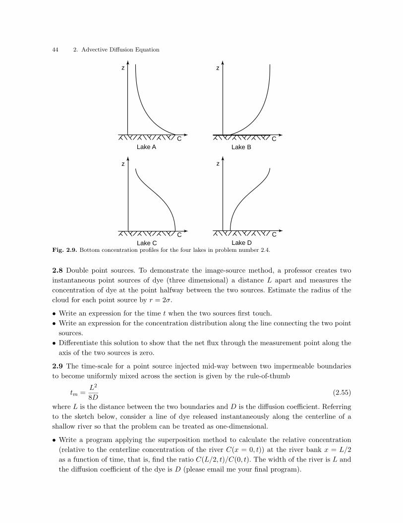
2.7 Concentration profiles. Figure 2.9 shows four concentration profiles measured very carefully

at the bottom of four different lakes. For each profile, state whether the lake bottom is a no-flux

or flux boundary and describe where you think the source is located and why.


z

Lake CC

z

Lake DC

z

Lake AC

z

Lake BC

Fig. 2.9. Bottom concentration profiles for the four lakes in problem number 2.4.

2.8 Double point sources. To demonstrate the image-source method, a professor creates two

instantaneous point sources of dye (three dimensional) a distance L apart and measures the

concentration of dye at the point halfway between the two sources. Estimate the radius of the

cloud for each point source by r = 2σ.

• Write an expression for the time t when the two sources first touch.

• Write an expression for the concentration distribution along the line connecting the two point

sources.

• Differentiate this solution to show that the net flux through the measurement point along the

axis of the two sources is zero.

2.9 The time-scale for a point source injected mid-way between two impermeable boundaries

to become uniformly mixed across the section is given by the rule-of-thumb

tm =L2

8D(2.55)

where L is the distance between the two boundaries and D is the diffusion coefficient. Referring

to the sketch below, consider a line of dye released instantaneously along the centerline of a

shallow river so that the problem can be treated as one-dimensional.

• Write a program applying the superposition method to calculate the relative concentration

(relative to the centerline concentration of the river C(x = 0, t)) at the river bank x = L/2

as a function of time, that is, find the ratio C(L/2, t)/C(0, t). The width of the river is L and

the diffusion coefficient of the dye is D (please email me your final program).

Exercises 45

• Plot your result with C(L/2, t)/C(0, t) as the y-axis and t/(L2/D) as the x-axis using the

values L = 10 m and D = 0.01 m2/s.

• What is the relative concentration when t = tm?

x = -L/2 x = L/2x = 0

2.10 How is the three-dimensional point-source solution derived. You don’t need to show the

details of the derivation. Just explain the methodology with a minimum number of equations.

2.11 Smoke stack. A chemical plant has a smoke stack 75 m tall that discharges a continuous

flux of carbon monoxide (CO) of 0.01 kg/s . The wind blows with a velocity of 1 m/s due east

(from the west to the east) and the transverse turbulent diffusion coefficient is 4.5 m2/s. Neglect

longitudinal (downwind) diffusion.

• Write the unbounded solution for a continuous source in a cross wind.

• Add the appropriate image source(s) to account for the no-flux boundary at the ground and

write the resulting image-source solution for concentration downstream of the release.

• Plot the two-dimensional concentration distribution downstream of the smoke stack for the

plane 2 m above the ground.

• For radial distance r away from the smoke stack, where do the maximum concentrations occur?

2.12 Damaged smoke stack. After a massive flood, the smoke stack in the previous problem

developed a leak at ground level so that all the exhaust exits at z = 0.

• How does this new release location change the location(s) of the image source(s)?

• Plot the maximum concentration at 2 m above the ground as a function of distance from the

smoke stack for this damaged case.

• If a CO concentration of 1.0 µg/l of CO is dangerous, should the factory be closed until repairs

are completed?

2.13 Boundaries in a boat arena. A boat parked in an arena has a sudden gasoline spill. The

arena is enclosed on three sides, and the spill is located as shown in Figure 2.10. Find the

locations of the first 11 most important image sources needed to account for the boundaries and

incorporate them into the two-dimensional instantaneous point-source solution.

2.14 Image sources in a pipe. A point source is released in the center of an infinitely long round

pipe. Describe the image source needed to account for the pipe walls.


Open boundary

x

y

(0,0)

L(0.5L,0.75L)

Spill

No-flux boundariesFig. 2.10. Sketch of the boat arena and spill location for problem number 2.4.

2.15 Vertical mixing in a river. Wastewater from a chemical plant is discharged by a line diffuser

perpendicular to the river flow and located at the bottom of the river. The river flow velocity is

15 cm/s and the river depth is 1 m.

• Find the locations of the first four most important image sources needed to account for the

river bottom and the free surface.

• Write a spreadsheet program that computes the ratio of C(x, z = h, t = x/u) to Cmax(t =

x/u), where u is the flow velocity in the river and h is the water depth; x = z = 0 at the

release location.

• Use the spreadsheet program to find the locations where the concentration ratio is 0.90, 0.95,

and 0.98.

• From dimensional analysis we can write that the time needed for the injection to mix in the

vertical is given by

tmix =xmix

u=

h2

αD(2.56)

where D is the vertical diffusion coefficient. Compute the value of α for the criteria Cmin/Cmax =

0.95.

• Why is the value of α independent of D?

2.16 Mixing of joining rivers. One river (left) with a high concentration of sediment joins another

river (right) with a negligible sediment concentration. The width of the low concentration river

near their union is 40 m while the high concentration river is 80 m wide. Assume the river width

and depth do not change much after the union, and both rivers are shallow and have the same

velocity. At one particular day the mean velocity downstream of the union is 1 m/s and the

diffusion coefficient is 0.1 m2/s.

• Estimate the time required tmix and the distance downstream xmix until the low sediment con-

centration river is considered to be well-mixed with the sediment from the high concentration

river. Use a relative concentration of 95% as the criteria for the well-mixed condition.

• If there is a water intake located on the low-sediment side of the river at 3 km downstream

from the river union, do you expect the water taken from the intake to contain a significant

amount of sediment? Justify your answer.

Exercises

47

Table 2.1: Table of solutions to the diffusion equation

Schematic and Solution

Instantaneous point source, infinite domain

C

x

C(x,t = 0) =

x0

δ (x-x0)MA

8

C

x

Cmax

2σ1

4σ2

C(x, t) =M

A√

4πDtexp

[

− (x − x0)2

4Dt

]

Cmax(t) =M

A√

4πDt

qx(x, t) =M(x − x0)

2At√

4πDtexp

[

− (x − x0)2

4Dt

]

Let σ =√

2Dt and(2σ)2 = 8Dt.For x0 = 0:C(±σ, t) = 0.61Cmax(t)

Let σ =√

2Dt and(4σ)2 = 32Dt.For x0 = 0:C(±2σ, t) = 0.14Cmax(t)

Instantaneous distributed source, infinite domain

C

x

C(x,t = 0) =

x0

C

x

2σ1

C0, x < x0

0, x > x0

C02

4σ2

C(x, t) =C0

2

[

1 − erf

[

(x − x0)√4Dt

]]

Cmax(t) = C0

qx(x, t) =C0

√D√

4πtexp

[

− (x − x0)2

4Dt

]

Let σ =√

2Dt and(2σ)2 = 8Dt.For x0 = 0:C(+σ, t) = 0.16C0

C(−σ, t) = 0.84C0

Let σ =√

2Dt and(4σ)2 = 32Dt.For x0 = 0:C(+2σ, t) = 0.02C0

C(−2σ, t) = 0.98C0

48

2.

Advectiv

eD

iffusio

nE

quatio

nTable 2.1: (continued)

Schematic Solution

Fixed concentration, semi-infinite domain

C

x

C(x=x0,t ) = C0

x0

C

x

σ

C0

C0

2σ

C(x > x0, t) = C0

[

1 − erf

[

(x − x0)√4Dt

]]

Cmax(t) = C0

qx(x > x0, t) =2C0

√D√

4πtexp

[

− (x − x0)2

4Dt

]

Let σ =√

2Dt andσ2 = 2Dt.For x0 = 0:C(+σ, t) = 0.32C0

C(−σ, t) = Undefined

Let σ =√

2Dt and(2σ)2 = 8Dt.For x0 = 0:C(+2σ, t) = 0.05C0

C(−2σ, t) = Undefined

Instantaneous point source, bounded domain

C

x

C(x,t = 0) =

x0

δ (x-x0)MA

8

C

x

Cmax

dCdx

= 0xb

2Lb

C(x, t) =M

A√

4πDt

∞∑

n=−∞

exp

[

− (x − x0 + 2nLb)2

4Dt

]

Cmax(t) =M

A√

4πDt

∞∑

n=−∞

exp

[

− (2nLb)2

4Dt

]

qx(x, t) =M

2At√

4πDt

∞∑

n=−∞

(x − x0 + 2nLb) exp

[

− (x − x0 + 2nLb)2

4Dt

]

Using the image-sourcemethod, the first imageon the opposite side ofthe boundary is atx0 ± 2Lb.

Exercises

49

Table 2.1: (continued)

Schematic Solution

Instantaneous 2-D point source, infinite domain

y

x

C(x,y,t = 0) = δ (x-x0)MH

y

x

δ (y-y0)

(x0,y0)

σ

C(x, y, t) =M

4πHt√

DxDy

exp

[

− (x − x0)2

4Dxt

− (y − y0)2

4Dyt

]

Cmax(t) =M

4πHt√

DxDy

q(x, y, t) =M

8πHt2√

DxDy

exp

[

− (x − x0)2

4Dxt

− (y − y0)2

4Dyt

]

((x − x0)i + (y − y0)j)

Let Dx = Dy,σ =√

2Dt,(2σ)2 = 8Dt, andr2 = (x−x0)

2+(y−y0)2.

For r = σ:C(σ, t) = 0.61Cmax(t)

Let Dx = Dy,σ =

√2Dt,

(4σ)2 = 32Dt, andr2 = (x−x0)

2+(y−y0)2.

For r = 2σ:C(2σ, t) = 0.14Cmax(t)

Instantaneous 3-D point source, infinite domain

z

x

C(x,y,t = 0) = δ (x-x0)MH

z

x

δ (y-y0)

(x0,y0,z0)

δ (z-z0)

Iso-concentrationsurface

y

y

C(x, y, z, t) =M

4πt√

4πtDxDyDz

exp

[

− (x − x0)2

4Dxt

− (y − y0)2

4Dyt− (z − z0)

2

4Dzt

]

Cmax(t) =M

4πt√

4πtDxDyDz

q(x, y, z, t) =M

8πt2√

4πtDxDyDz

exp

[

− (x − x0)2

4Dxt

− (y − y0)2

4Dyt− (z − z0)

2

4Dzt

]

·

((x − x0)i + (y − y0)j + (z − z0)k)

Let Dx = Dy = Dz,σ =

√2Dt, (2σ)2 = 8Dt,

andr2 = (x − x0)

2 + (y −y0)

2 + (z − z0)2.

For r = σ:C(σ, t) = 0.61Cmax(t)

Let Dx = Dy = Dz,σ =

√2Dt,

(4σ)2 = 32Dt, andr2 = (x − x0)

2 + (y −y0)

2 + (z − z0)2.

For r = 2σ:C(2σ, t) = 0.14Cmax(t)

lecture 12: advection and diffusion in environmental flows · lecture 12: advection and diffusion...

Documents