a general-purpose finite-volume advection … general-purpose finite-volume advection scheme for...

Journal of Computational Physics 180, 559–583 (2002)doi:10.1006/jcph.2002.7105

A General-Purpose Finite-Volume AdvectionScheme for Continuous and Discontinuous

Fields on Unstructured Grids

E. D. Dendy, N. T. Padial-Collins, and W. B. VanderHeyden

Los Alamos National Laboratory, Theoretical Division, Fluid Dynamics Group (T-3), and Los AlamosComputer Science Institute, Los Alamos, New Mexico 87545

E-mail: [email protected], [email protected], and [email protected]

Received March 30, 2001; revised April 1, 2002

We present a new general-purpose advection scheme for unstructured meshesbased on the use of a variation of the interface-tracking flux formulation recently putforward by O. Ubbink and R. I. Issa (J. Comput. Phys. 153, 26 (1999)), in combi-nation with an extended version of the flux-limited advection scheme of J. Thuburn(J. Comput. Phys. 123, 74 (1996)), for continuous fields. Thus, along with a high-order mode for continuous fields, the new scheme presented here includes optionalintegrated interface-tracking modes for discontinuous fields. In all modes, the methodis conservative, monotonic, and compatible. It is also highly shape preserving. Thescheme works on unstructured meshes composed of any kind of connectivity element,including triangular and quadrilateral elements in two dimensions and tetrahedral andhexahedral elements in three dimensions. The scheme is finite-volume based and isapplicable to control-volume finite-element and edge-based node-centered computa-tions. An explicit–implicit extension to the continuous-field scheme is provided onlyto allow for computations in which the local Courant number exceeds unity. Thetransition from the explicit mode to the implicit mode is performed locally and in acontinuous fashion, providing a smooth hybrid explicit–implicit calculation. Resultsfor a variety of test problems utilizing the continuous and discontinuous advectionschemes are presented. c© 2002 Elsevier Science (USA)

Key Words: advection; reconstruction; interface tracking; volume of fluid; unstruc-tured meshes; unstructured grids; finite-volume method.

1. INTRODUCTION

The development of accurate, conservative, monotonic, compatible, shape-preservingnumerical advection schemes has been the subject of intense study for several decades.Despite this effort, the quest for improved techniques continues. Leveque [5] provides an

559

0021-9991/02 $35.00c© 2002 Elsevier Science (USA)

All rights reserved.

560 DENDY, PADIAL-COLLINS, AND VANDERHEYDEN

extensive survey of the literature on this topic. Let us begin our discussion here with somedefinitions. In this paper conservative denotes an advection scheme that guarantees no lossof conserved quantities, such as mass, in the operation of moving material from one conser-vation volume to another under the action of advection. We use the modifier monotonic todenote an advection operator or scheme, which does not produce any unphysical extremain the updated density field. This property is also sometimes referred to as total variationdiminishing, or TVD. Similarly, we use the modifier compatible to denote an advectionoperator or scheme which does not produce any unphysical extrema in the updated mass-specific or “mixing ratio” quantities, such as specific internal energy or velocity. Finally,we use the modifier shape preserving to refer to a scheme that minimizes the distortionof the shape of features in the conserved field in multidimensional flows. An advectionscheme that is shape preserving is sometimes also said to provide corner coupling. Thistypically means that material from a given donor cell is transported, in a single applicationof the advection scheme, to a neighboring cell, or “corner cell,” which has only a vertexin common with the donating cell. Doing this corner-cell transport correctly leads to shapepreservation. All of these characteristics are essential for accurate Eulerian flow physicssimulation schemes.

Our goal here is to provide an advection scheme that is conservative, monotonic, com-patible, and shape preserving for the cases of both continuous and discontinuous densityfields in an integrated treatment. Furthermore, our goal is also to provide this scheme forunstructured grids. An example of the continuous-field case emerges in the simulation of alow Mach number compressible gas flow where the mass density fields, for example, aresmooth continuous functions of space. An example of the discontinuous case would be thesimulation of a free surface flow such as the sloshing of a liquid in a partially filled tank. Suchan integrated scheme would be an attractive candidate in many of today’s general-purposeflow simulation software, particularly those that address multimaterial and multifield flowproblems.

Thus, we present in this paper a new general-purpose advection scheme for unstructuredmeshes based on the use of an interface-tracking flux formulation recently put forward byUbbink and Issa [10], in combination with an extended version of the flux-limited advectionscheme of Thuburn [8], for continuous fields. In what follows, we provide a brief reviewof the key features of the methods of Thuburn and Ubbink and Issa. Following this, weoutline our scheme and then provide results on a variety of advection examples to showits accuracy and robustness. The examples include continuous-field advection, interfacetracking, and explicit–implicit advection on quadrilateral and triangular element grids (alltreated internally as unstructured grids). We conclude with a discussion of future work,including an outline of the use of our scheme in a continuous-remapping, Lagrangian–Eulerian scheme to accommodate right-hand-side physics.

2. OVERVIEW OF PRIOR WORK

Thuburn [8] developed a multidimensional flux-limiting scheme which ensures mono-tonic, compatible continuum advection with shape preservation. A key aspect of Thuburn’smethod is his criterion for the selection of limiting values for fluxed quantities based oninformation from both face and vertex neighbors. The inclusion of the vertex neighborvalues provides the shape-preservation or corner-coupling properties of his scheme. Another

A GENERAL-PURPOSE FINITE-VOLUME SCHEME 561

powerful aspect of Thuburn’s method derives from the fact that as a flux-limiting scheme,it can accommodate a wide variety of fluxed field reconstruction techniques. Thuburn useda third-order UTOPIA scheme appropriate to structured meshes for many of his examplecalculations. However his limiting scheme accommodates the use of alternatives. We willexploit this flexibility in the scheme presented in this paper and provide a simplification toThuburn’s limiting procedure that makes it computationally more efficient on unstructuredgrids.

Thuburn’s scheme also ensures the compatibility of mixing ratio quantities such as tem-perature and velocity, so it is applicable to a wide variety of applications. Finally, Thuburndescribes how his scheme can be used on quantities such as mass density, which can ex-hibit new extrema as the result of nonsolenoidal transport velocity fields. Thus, the Thuburnscheme can be applied to virtually any advection task in a coupled simulation involving con-servation of mass, momentum, energy, etc. Our second extension of the Thuburn’s schemewill be to regularize his advection and limiting equations so that they maintain compatibilityeven in the limit of vanishing mass density. This extension is particularly important for thecases of multimaterial and multifield flow simulations.

Following up on the original volume-of-fluid (VOF) scheme of Hirt and Nichols [3], andon ideas for compressive reconstruction by Gaskell and Lau [2], Ubbink and Issa [10] haverecently published a novel interface-tracking scheme. In their method they compute fluxedquantities from a weighted average of estimates based on continuous-field reconstructionand one based on simple compressive reconstruction. Ubbink and Issa’s weighting factor isbased on the angle between the interface surface normal and the conservation cell face sur-face normal and is astutely chosen to avoid the interface-wrinkling effects seen in previousversions of the VOF method. Ubbink and Issa use this reconstruction strategy for the com-putation of fluxed quantities inside a Crank–Nicholson time discretization of the advectionoperator to provide good shape preservation properties for interface-tracking simulations.To enforce monotonicity, they introduce a correction step to their scheme applied aftereach successive solution of the Crank–Nicolson system until they have a monotone futurefield.

We have developed two variations of the Ubbink–Issa method for use in our general–purpose scheme. Our first variation is completely explicit; the second utilizes Ubbink andIssa’s Crank–Nicolson scheme. For the explicit scheme, we first modify the Ubbink–Issaflux quantity formulation to include our multidimensional continuous-field flux formula-tion in place of their use of the ULTIMATE-QUICKEST [4], high-order, one-dimensionalformulation. This allows us to integrate our interface-tracking formulation neatly with ourcontinuous-field formulation. We find that this formulation works well on both triangu-lar and quadrilateral element meshes. In this mode, we apply our modified version ofThuburn’s multidimensional limiter to ensure monotonicity. In our second variation, weuse Ubbink and Issa’s Crank–Nicolson approach to obtain the fluxed quantities and re-place their iterative correction with an application of our modified version of Thuburn’slimiter. This yields bounded future values without the need for an iterative correctionscheme to enforce monotonicity. Thus, the properties of conservation, monotonicity, com-patibility, and shape preservation are enforced simultaneously with the solution of theequations.

Finally, we also develop in our scheme an explicit/implicit capability by coupling ourflux formulations for low Courant numbers to a fully implicit flux formulation, in a smoothfashion, to provide a continuously applicable method for virtually all Courant numbers.


3. ADVECTION SCHEME

In the scheme presented in this paper, we adopt and extend the flux-limiting scheme ofThuburn. We use both continuous-field reconstruction and our two modified versions ofthe reconstruction strategy of Ubbink and Issa to provide an integrated advection schemeapplicable to both continuous-field advection and interface tracking for a wide variety ofapplications. For maximum flexibility, we provide some modest extensions to the Thuburnlimiting scheme to accommodate fully unstructured grids and smooth compatible advectioneven in the limit of vanishing mass densities.

3.1. Conservation Equations

Without sacrificing generality, we start with the following prototypical pure-advectionconservation system for mass with density � and an additional conserved quantity withdensity �q . The equations are

∂�

∂t+ ∇ · (� �u) = 0 (1)

and

∂�q

∂t+ ∇ · (�q�u) = 0. (2)

Here �u is the velocity field and q is a mass specific quantity sometimes called a mixingratio. It is useful to consider the advective forms of these equations. Equation (1) can bewritten as

D�

Dt= −�∇ · �u, (3)

and Eq. (2) as

Dq

Dt= 0, (4)

where

D

Dt≡ ∂

∂t+ �u · ∇

is the familiar material derivative which gives the time rate of change following the materialmotion. We can now more precisely discuss the concepts of monotonicity and compatibility.First, from Eq. (3) we can see that only velocity divergence can cause changes in massdensity. So a monotonic advection scheme is one that does not introduce any artificialextrema into the mass density field due to numerical inaccuracies. In particular, for the caseof incompressible or divergence-free velocity fields, a monotonic field should ensure thatno new mass density extrema are created.

As for compatibility, we can see from Eq. (4) that mixing ratio quantities should remainconstant following the fluid motion even for cases in which the velocity field has a diver-gence. Thus a compatible advection scheme is one in which no new extrema are artificially


created due to numerical inaccuracies even for the cases in which the velocity divergenceis nonzero.

We now develop the discrete finite-volume versions of Eqs. (1) and (2). In preparation,let us define several quantities. Let Vk be the volume corresponding to the kth node of agiven mesh. Let the average mass density and mixing ratio for that node be defined as

�k ≡ 1

Vk

∫Vk

� dV ,

qk ≡ 1

�k Vk

∫Vk

�q dV .

Then, following Thuburn, we can integrate Eqs. (1) and (2) over the control volume and, overa time interval, apply the divergence theorem and discretize the resulting surface integralsto obtain the finite-volume versions of Eqs. (1) and (2),

�m+1k = �m

k +∑

f

Cink− f �̂ f −

∑f

Coutk− f �̂ f (5)

and

�m+1k qm+1

k = �mk qm

k +∑

f

Cink− f �̂ f q̂ f −

∑f

Coutk− f �̂ f q̂ f , (6)

respectively. The superscripts m and m + 1 denote the known and unknown time levels,respectively, separated by a time interval, �t . The summations in Eqs. (5) and (6) arecarried out over all faces of the control volume. The quantities Cin

k− f and Coutk− f are inflow

and outflow Courant numbers for face f of the kth control volume and are defined as

Cink− f = H (−�u f · n̂k− f )

V̂ f

Vk(7)

and

Coutk− f = H (�u f · n̂k− f )

V̂ f

Vk, (8)

where H is the Heaviside function, �u f is the average velocity on face f , n̂k− f is the outwardsurface unit normal of face f for the kth control volume, and V̂ f is the volume of materialthat passes through face f over the time interval �t given by the formula

V̂ f = �t |�u f · n̂ f |A f , (9)

where A f is the area of face f and n̂ f is either one of the face normal vectors for theadjacent control volumes. The quantity V̂ f is often referred to as the flux volume.

The quantities �̂ f and q̂ f in Eqs. (5) and (6) are the average values of the � and q overthe flux volumes for face f. We will refer to these quantities as fluxed values or fluxedquantities.


In order to compute the updated values of q we follow Thuburn [8] and divide the left-and right-hand side of Eq. (5) into the respective left and right sides of Eq. (6) and thendivide the resulting right-hand side numerator and denominator by �m

k to obtain

qm+1k = qm

k + ∑f Cin

k− f

(�̂ f

/�m

k

)q̂ f − ∑

f Coutk− f

(�̂ f

/�m

k

)q̂ f

1 + ∑f Cin

k− f

(�̂ f

/�m

k

) − ∑f Cout

k− f

(�̂ f

/�m

k

) . (10)

Equation (10) is the final update formulation presented by Thuburn [8] for the mixing ratioquantity. While this form was suitable to Thuburn’s purposes, we must modify it in orderto ensure smooth calculations in the limit as �m

k → 0. This limit is ubiquitous in multifieldflows. Consider, for example, the simple case of a sedimenting two-phase flow. The densityof the settling material is zero above the two-phase region. In computations of such a flow,we would like mixing ratio quantities to take on sensible values and not simply “blow up.”Accordingly, we recast Eq. (10) by extracting qm

k from the right-hand side as a separateterm and then by multiplying the numerator and denominator of the remainder by �m

k . Thisleaves Eq. (10) in the form

qm+1k = qm

k +∑

f Cink− f �̂ f

(q̂ f − qm

k

) − ∑f Cout

k− f �̂ f(q̂ f − qm

k

)�m+1

k + ε. (11)

Here we have used Eq. (5) to further simplify the denominator of the second right-hand-sideterm. Note that we have also added the quantity ε to the denominator of the second termin Eq. (11). This is intended to be a small positive parameter that will be used to preventdivision by zero in numerical computations. Now consider what happens in the event of�m+1

k approaching zero. In this case, as long as the numerator of the second right-hand-sideterm approaches zero, the mixing ratio, qk , will simply not change. This is automatic forthe cases in which both inflow and outflow masses are zero. For other cases, this desirablebehavior will emerge from the application of Thuburn’s flux limiter with a few minorextensions. This is the subject of the next section.

3.2. Modified Thuburn Flux Limiter

In this section we discuss our modifications to Thuburn’s flux limiter for the fluxedquantities in Eq. (11). Since Thuburn’s limiting procedure is indifferent to the method used tocompute fluxed quantities, we delay discussion of the formulations for the unlimited fluxedquantities to the next section. Note that, as Thuburn [8] teaches, his flux limiter can be usedto limit both the mass density fluxed values, �̂ f , as well as the mixing ratio fluxed values,q̂ f . We continue to use this approach. We will elaborate more on this later. For now, wewill discuss our modifications to Thuburn’s limiting scheme to accommodate unstructuredmeshes and to allow for vanishing mass densities. We will confine our attention here onlyto our modifications and point the reader to Thuburn’s paper [8] for the full explanation ofhis method.

3.2.1. Upstream-neighbor effects. The first modification of Thuburn’s limiting proce-dure that we have introduced generalizes a particular aspect of his method to unstructuredgrids. One of the steps in Thuburn’s limiting procedure involves widening the limitingbounds on fluxed quantities to reflect contributions from inflows from control volumes ad-jacent to the control volume upwind from a given face. This is the part of Thuburn’s scheme


that provides the shape-preservation characteristics. In Thuburn’s original prescription, onlyface neighbors from the upwind control volume that had a common vertex with the flux facein question were included. Thus, for a quadrilateral, the face neighbor opposite the flux facein question was excluded. For unstructured meshes, this exclusion, while not impossible, isquite onerous. It is much easier in, for example, the edge-based data structures that we usedin many of our computations to simply include the effect of all face neighbors from the up-stream control volume. This allowed us to accumulate the upstream-neighbor information ateach node about upstream-face or, equivalently, edge-neighbor values simply using a sweepthrough all mesh edges. Then, when performing Thuburn’s technique of widening boundson fluxed quantities for a given face, we can simply look to this accumulated informationon the upwind node for the face. We found that our results were not affected by includingthis additional information.

3.2.2. Protection against division by zero in the limiter. The second modification toThuburn’s limiting procedure is introduced to protect against division-by-zero problemswhen no outflow exists. Thuburn provides formulas for bounds on outflow fluxed quantitiesusing the conservation equations and information from surrounding neighbor node data.Our alternative forms for these formulas are

(q̂ (out)

k

)min = qm

k +∑

f

{C in

k− f �̂ f[(

q (in)f

)max − qm

k

]} − {(qm+1

k

)max − qm

k

}�m+1

k∑f Cout

k− f �̂ f + ε, (12)

(q̂ (out)

k

)max = qm

k +∑

f

{C in

k− f �̂ f[(

q (in)f

)min − qm

k

]} − {(qm+1

k

)min − qm

k

}�m+1

k∑f Cout

k− f �̂ f + ε, (13)

where (q̂ (out)k )min and (q̂ (out)

k )max are the minimum and maximum bounds for the outflow fluxedvalues for q for the kth control volume that ensure compatible advection. The quantities(q (in)

f )max and (q (in)f )min are the maximum and minimum inflow values for the fluxed quantities

for face f based on upstream data, including the effect of the nodes adjacent to upstreamcontrol volumes, as discussed in [8], and including our own modifications, discussed inSection 3.2.1 of this paper. Finally, (qm+1

k )max and (qm+1k )min are the maximum and minimum

future values for the quantity q based on the values from upstream neighbors [8].With the exception of the additional term, ε, in the denominators of Eqs. (12) and (13),

these equations are algebraically identical to Eqs. (42) and (43) in [8]. (Note, the smallquantity ε in Eqs. (12) and (13) is not necessarily the same as the ε in Eq. (11).) In ourform, we have separated the right-hand side into two parts: the first being the time m value,qm

k , which would correspond to explicit donor-cell advection, and the second containingthe high-order correction. We have added the small positive quantity ε to the denominatorsimply to protect from division by zero in machine computations when no outflow exists.In this limit, (q̂ (out)

k )max and (q̂ (out)k )min may have large values but will not be used since there

is no ouflow.

3.2.3. Clipping to enforce future bounds. In principle, the use of Thuburn’s limiter withthe extensions outlined above should result in computed future values of q that are boundedby (qm+1

k )max and (qm+1k )min, that is, compatible. In practice, particularly for the case of

vanishing mass densities, we have found that round-off errors can produce unboundedresults. We therefore introduce an additional step to Thuburn’s scheme after the updateusing Eq. (11), which clips any result that is out of bounds. We feel justified in doing


this because the results should be bounded. Any bounds violation is due only to round-offproblems. Specifically, we perform the following operations at each node:

qm+1k → min

[qm+1

k ,(qm+1

k

)max

]

and

qm+1k → max

[qm+1

k ,(qm+1

k

)min

].

This then provides a compatible advection scheme. This only seems necessary in the limitof vanishing mass density and thus should not introduce any substantial conservation errors.

3.3. Limiting Mass Densities for Monotonic Advection

As Thuburn has pointed out [8], we can use his limiting scheme to place bounds on thefluxed mass densities themselves to avoid unphysical extrema. Thuburn’s strategy is simplyto replace q with � and the product C �̂ with C in his limiting procedure. (Here C standsfor either Cin

k− f or Coutk− f .) By doing this, the limited mass densities are bounded by the

surrounding mass density data after including the effects of compression and expansion bythe divergent velocity field. The same strategy applies to our modified version of Thuburn’slimiter presented above.

3.4. Fluxed Quantity Formulation

Now that we have outlined our modifications to the Thuburn limiting scheme, we arein a position to discuss our formulation for the computation of the flux quantities beforelimiting. Our approach here is first to provide an alternative to the third-order UTOPIAscheme used by Thuburn to one that is more appropriate to unstructured grids. Followingthis we then provide an overview of our modified version of the Issa–Ubbink flux formulationfor interface-tracking computations.

3.4.1. Continuous field flux formulation. For the examples considered in this paper, weapproximate the variation of a given field, �, in the kth control volume as a linear function,

�k(�x) =�k + (∇�)k · (�x − �xk) + · · · , (14)

where �k is the average value of � in the control volume, (∇�)k is its gradient, and �xk is thecell centroid. The use of the linear function (14) provides more accuracy than a first-orderdonor cell scheme, as is well-known. We therefore term this our higher order formulation.Note also that we are not limited to a linear function; the formulation admits even higherorder expressions. Finally, note that for some meshes, �xk is not always the same as theposition of the node. In the examples that follow, for simplicity, we used the node positioninstead of the centroid and accept the error. We then obtain an estimate of the average valueof � in the flux volume by evaluating Eq. (14) at a point half way up the characteristic (backin time) following the fluid motion from the centroid of the face f, �x f . That is,

�̂ f =�u

(�x f − 1

2�u�t

), (15)

where the subscript u denotes the upwind control volume.


The gradient in Eq. (14) must be supplied to the method by some suitable numericaldifferencing scheme. In our work we used a simple, so-called, Green–Gauss method

(∇�)k ≈ 1

Vk

∑f

� f A f �nk− f , (16)

where the quantity � f is the average value of � for face f . We employ two methods tocompute this average value from surrounding nodal data. In the first method, we simply usethe average of the two node values across the face f . In the second method, we computeaverage values of � for each of the vertices of face f . These vertex values are computedas averages of local surrounding data. Since each face vertex corresponds to a unique meshelement and is approximately at the center of this element, we use the element node dataas the surrounding data. These face vertex values are then averaged with the two valuesacross the face to give the final face value. For example, the first method corresponds to afive-point stencil on structured quadrilaterals, while the second method corresponds to thatof a nine-point stencil.

This approach is general and works for all element types. In our computations, thefirst method was used for continuous-field advection and the second method was used forinterface tracking advection. This was done because we found that the second method gaveimproved shape preservation properties to the interface tracking calculations.

3.4.2. Discontinuous-field flux formulation. We now address the case of discontinuousfields. Specifically, we are interested in cases in which we are trying to track interfaces inour calculations. In these cases, the discontinuous-field is a volume fraction. In multifieldflow simulations, the volume fraction, �, is related to the conserved macroscopic density,� , and the microscopic intrinsic material density, �o as � = �/�o. We now discuss ourmodified formulation of the Ubbink–Issa formulation for volume fraction fluxes, �̂. Oncethese volume fraction fluxes are computed we may then reconstruct the mass density fluxesas �̂ = �̂�̂o.

3.4.3. Modified Ubbink–Issa formulation. Let us now consider directly the flux formu-lation for a volume fraction field. We assume that we are completely resolving materialinterfaces and the volume fraction is either 0 or 1 at any point in space in the continuouslimit. Of course, in the numerical calculation, the average volume fraction in a controlvolume can be fractional if the volume is only partially filled with the material in question.This means that the nodal values for volume fraction can vary continuously between 0 and1 over three contiguous control volumes. This is the case that Ubbink and Issa [10] haverecently addressed.

The original VOF method by Hirt and Nichols [3] made use of the combination of acompressive reconstruction and a continuous-field reconstruction in order to maintain thesharp step profile of a discontinuous-field such as a fluid interface. Ubbink and Issa [10]recently provided a very effective means of smoothly varying between the compressiveand continuous-field schemes by taking the weighted average between the two. They makeuse of a locally bounded, one-dimensional, differencing scheme first described by Gaskelland Lau [2] for the compressive reconstruction, and Leonard’s one-dimensional, high-orderULTIMATE-QUICKEST [4] for their continuous-field reconstruction. The weighting be-tween the compressive and continuous-field reconstruction is a function of the angle betweeninterface normal vectors, as determined from upstream volume fraction gradients and cell


face normal vectors. Ubbink and Issa extend these hybrid one-dimensional treatments tomultiple dimensions by time centering the fluxed values using a Crank–Nicolson scheme.That is, they apply their hybrid flux formulation to the time m and m + 1 data separatelyand then average to obtain the final flux values for volume fraction that are used in theconservation equation. Thus, their method has an implicit component, so finding the timem + 1 solution requires a system solver. To enforce monotonicity, Ubbink and Issa applya correction between successive linear solutions to fix out-of-bounds values. For a moredetailed description of their algorithm see [9, 10].

We employ the bulk of Ubbink and Issa’s scheme here in our general-purpose frame-work. We make, however, two separate modifications to produce two alternative variationsmore suitable to our needs. In the first variation, we replace the use of the ULTIMATE-QUICKEST, one-dimensional high-order formulation for the continuous-field flux valuewith our multidimensional reconstruction scheme outlined above. We then use a weightingof this high-order flux value, �̂ho, with the one-dimensional compressive, �̂c, reconstructionas outlined in [10],

�̂ f = ��̂c + (1 − �)�̂ho. (17)

The weighting � [10] varies smoothly between 1 and 0 as the angle between the facenormal and the interface normal varies between 0 and 90◦. We then use this flux formu-lation in a fully explicit mode and employ our modified version of Thuburn’s limiter onthe resulting fluxed values, �̂ f , to ensure monotonocity. In our second variation of theUbbink–Issa scheme, we use a slightly modified version of their Crank–Nicolson formula-tion wherein we replace their iterative correction scheme with an a posteriori applicationof our modified version of Thuburn’s limiting scheme [8], ensuring only one linear solutionper time step. In the remainder of this paper the first method will be referred to as the“explicit” scheme while the latter will be referred to as the “implicit” or “Crank–Nicolson”scheme.

In Ubbink and Issa’s scheme, the volume fraction flux is computed as a weighted averageof the upwind and downwind node volume fractions

�̂ f = (1 − � f )�D + � f �A, (18)

where �D and �A are the downwind and upwind node volume fractions. The weight factor� f is a complicated function of the surrounding volume fractions and the material interfaceand control volume face surface unit normal vectors [10]. In order to avoid introducing anonlinear system for the new time volume fraction, Ubbink and Issa advocate time laggingthe weight factors in their Crank–Nicolson formulation for multidimensional computations.Thus, their final expression for the fluxed volume fraction is

�̂ f = (1 − � f )�m

D + �m+1D

2+ � f

�mA + �m+1

A

2, (19)

where � f is evaluated with time m data. Ubbink and Issa imply that the fully nonlinearfluxing value, with � f values evaluated with both time m and m + 1 data, would actuallydo a better job of representing the time average of volume fluxes through a given timestep. We initially implemented the full nonlinear version. Since we are now routinely solv-ing nonlinear systems using the Jacobian–free Newton–Krylov solution methods [1], this


extension of their method did not place any additional requirements on our solution soft-ware. However, we did not see any appreciable additional benefit of the nonlinear fluxingvalues. Since the linear fluxing values are more computationally economical, we chose toretain these in our work.

We now deviate from [10], as mentioned above, by applying our modified version ofThuburn’s limiter to the resulting converged time-centered, Crank–Nicolson flux values fordensity. These limited fluxing quantities are then used to obtain the future values of densityfrom Eq. (5).

3.4.4. Explicit–implicit flux value formulation. Although we have not performed a VonNeumann stability analysis, our scheme appears to be stable as long as the sum of all outflowface Courant numbers is less than 1.0 for any node. We can, however, combine our explicitscheme with implicit schemes in order to compute at higher Courant numbers. We do thisby combining flux values computed using our high-order explicit formulation with explicitupwind and a fully implicit flux value in a smooth continuous fashion. Let us denote theexplicit first-order upwind flux value �̂f-donor, the implicit flux value �̂f-ss, and the limitedexplicit high-order continuous field flux �̂f-ho. In this paper, we used the upwind node timem + 1 value for �̂f-ss. Implicit donor-cell advection, while inaccurate, is known to be stablefor all Courant numbers. This choice can, of course, be generalized to more sophisticatedoptions in the future. Then our combined expression for the explicit–implicit fluxed valueis

�̂ f = �̂f-implicit + �̂f-explicit, (20)

where

�̂f-implicit = max

[0, 1 − Cmax

CD f

]�̂f-ss (21)

and where the explicit fluxed value is a combination of the explicit first-order and high-ordervalues

�̂f-explicit = min

[1,

Cmax

CD f

]{min

[1,

(CD f

Cmax

)�]�̂f-donor

+(

1 − min

[1,

(CD f

Cmax

)�])�̂f-ho

}, (22)

where CD f is the sum of all outflow Courant numbers for the upwind control volume forface f ,

CD f =∑

fu

CoutD− fu

. (23)

The quantity Cmax is introduced as a maximum value for the sum of the outflow face Courantnumbers, CD f , which can be controlled by the user. For stability Cmax should be set to avalue less than 1.0.

Equation (22) was obtained by blending the high-order and donor-cell fluxes so thatthe explicit flux tends toward the explicit donor-cell value as the Courant number sum,CD f , approaches Cmax. This is done to keep high-order flux values from introducing noise


as the evaluation point on the characteristic moves farther back and potentially outsidethe upstream control volume. The exponent � controls the rate of transition between thehigh-order flux values and the explicit donor value. As � approaches infinity the transitionbetween the two schemes becomes a step function with the change occurring abruptly atCD f equals Cmax. In our calculations we chose a value of � equals 50 to ensure a smoothtransition. This value for CD f delayed the onset of transition from high-order to first-orderupwind such that it occurred between Cmax − 0.05 and Cmax. In our calculations, we setCmax to 0.85, which is safely away from the apparent stability limit of 1.0 for the explicitpart of the scheme.

As an example of how this scheme works, consider the case CD f equals 2. For this casethe final fluxed quantity is weighted as 0.425 from the explicit donor cell and 0.575from the implicit value. Notice also that in the limit, as the Courant number tends to infinity,the explicit flux value tends to zero and the implicit flux value tends to the steady-stateflux value. This property can be exploited so that the advection scheme can work in both atime-dependent and a steady-state service (see Section 5).

4. RESULTS AND DISCUSSION

In this section we present several test cases that exhibit the accuracy of the variouscomponents of our new integrated advection scheme. In each of the examples the density,� , is updated at each time step with Eq. (5). In several of the examples we also compute atemperature field, q (with unit specific heat), that is transported with the material according toEq. (11). With this choice of variables, the product �q can be usefully considered a mixturetemperature. (For example, if we have the special case of a two-phase, nonconductingmixture, with each phase having unit microscopic material density, one phase with zerotemperature, and the other with temperature q, then �q would be the mixture temperature.) Inall cases, we compute with flux values computed with the reconstruction methods discussedin this paper and limit them with our modified version of Thuburn’s limiter [8]. We firstshow continuous-field advection on structured and unstructured meshes. Shape preservationon both quadrilateral and triangular element meshes is demonstrated. Our next two examplecalculations demonstrate the accuracy of our interface-tracking mode for the cases of simpletranslation and deformation in a vortical shear field. Both of these are common test problemsused in validating interface-tracking methods. The simple translation test case includes thetransport of a temperature field with the material as well. Here we demonstrate good shapepreservation as well as compatible advection of a mass specific quantity, temperature. Inthe case of vortical shear flow, under time reversal, we show that we essentially recoverthe initial conditions. Error norms from these simulations on quadrilateral and triangularelement meshes are tabulated along with those of [7, 10]. Finally, we show a computationof advection of concentration in a jet flow field, which shows the efficacy and utility of ourexplicit–implicit formulation.

Two domains, a unit square and a rectangle, have been used to compute the resultspresented in this section. Each domain is discretized, with structured quadrilateral elementsand unstructured triangular elements having approximately the same number of nodes.Figure 1 shows a coarse representative example of the types of triangular meshes used forthe example calculations in this paper. The quadrilateral meshes have a grid spacing of 0.01for the unit square and 0.02 for the rectangular mesh in each coordinate direction.


FIG. 1. Coarse representative example of a triangular element mesh.

4.1. Shape-Preserving Continuous-Field Advection

We first demonstrate the accuracy of our scheme for continuous-field advection on bothstructured quadrilateral and unstructured triangular grids. The domain for the computationis the unit square.

We start with an initial condition in which the density field is initialized with the distri-bution

� = 1

2

{1 + cos

[�√

(x − 0.2)2 + (y − 0.2)2

0.2

]for

√(x − 0.2)2 + (y − 0.2)2 < 0.2,

0 otherwise.

The temperature of this material is simply set to one where there is material and zero wherethere is not. That is,

T ={

1 for√

(x − 0.2)2 + (y − 0.2)2 < 0.2,

0 otherwise.

The existence of zero material density on the mesh provides us with a good test of ourmodifications to Thuburn’s limiter. At time zero, the material is subjected to a velocityfield along the diagonal of the unit square with unit velocities along the two coordinatedirections. The Courant number for these computations, based on the node volumes, was0.5. The computations were carried out over 240 time steps. The results of the computationsare shown in Figs. 2–7.

Figures 2 and 3 show the initial and final density resulting from advection using thepresent scheme and the first-order donor cell scheme. Figure 2 shows peak heights whileFig. 3 shows shape preservation. In both figures, a is the initial configuration, b is the resultusing the current scheme on the quadrilateral element mesh, c is the result using the currentscheme on the triangular element mesh, and d is the result for first-order donor cell as a


FIG. 2. Continuous-field advection results demonstrating peak preservation for density. (a) Initial condition;(b) quadrilateral element mesh results using current scheme; (c) triangular element mesh results using currentscheme; (d) quadrilateral element mesh results using first-order donor cell.

comparison. Figures 3a–3d show the same results in contour form. Here, for Figs. 3a–3c,the inner and outer contour values are 0.0625 and 0.9775 respectively. In Fig. 3d, wehave inner and outer contour values of 0.0625 and 0.5. The results in these figures showthe monotonicity, the good peak preservation, and the shape-preservation capabilities of thescheme.

As a point of reference for these results, we show in Fig. 3d the corresponding results for afirst-order upwind method on the quadrilateral mesh. These results show considerable peak

FIG. 3. Continuous-field advection results demonstrating shape preservation for density. (a) Initial condition;(b) quadrilateral element mesh results using current scheme; (c) triangular element mesh results using currentscheme; (d) quadrilateral element mesh results using first-order donor cell.


FIG. 4. Line contour plot of the final temperature field for quadrilateral mesh computation. The temperatureinside tightly packed contour lines is one; the temperature on the outside is zero.

height loss due to numerical diffusion and loss of shape. The percentage difference betweenthe initial and final peak values are 1.2, 1.5, and 45.4% for Figs. 2b–2d, respectively.

Figures 4 and 5 show line contour plots of the temperature fields, q, resulting fromthe advection computations. In each case, the temperature is one over the entire path of thematerial. This is expected by the design of our update, Eq. (11), which leaves the temperatureof a node unchanged if it empties or is empty. This is an artifact of having a zero-densitymaterial in the background. In a real multiphase flow calculation, for example, this sort ofthing would not happen because the temperature of the material outside the plume wouldbe dictated by the physics of the other material. We saw no compatibility problems with thetemperatures remaining bounded between zero and one.

A more useful way to look at the temperature in this case is to look at what we calledthe mixture temperature, �q , as shown in Figs. 6 and 7. The layout of these figures is thesame is in Fig. 2, with the exclusion of the donor cell results. In these figures, we see a morephysically intuitive temperature pattern with the mixture temperature nonzero only wherethe material is.


FIG. 5. Line contour plot of the final temperature field for triangular mesh computation. The temperatureinside tightly packed contour lines is one; the temperature on the outside is zero.

Finally, we also performed these computations on two unit square meshes with dis-cretizations twice and four times as coarse as the base meshes used in the above exam-ples. From these computations we obtained error norms which showed that the methoddisplays second-order convergence for both the quadrilateral and the triangular elementmeshes.

4.2. Compatible, Shape-Preserving Interface Tracking Advection

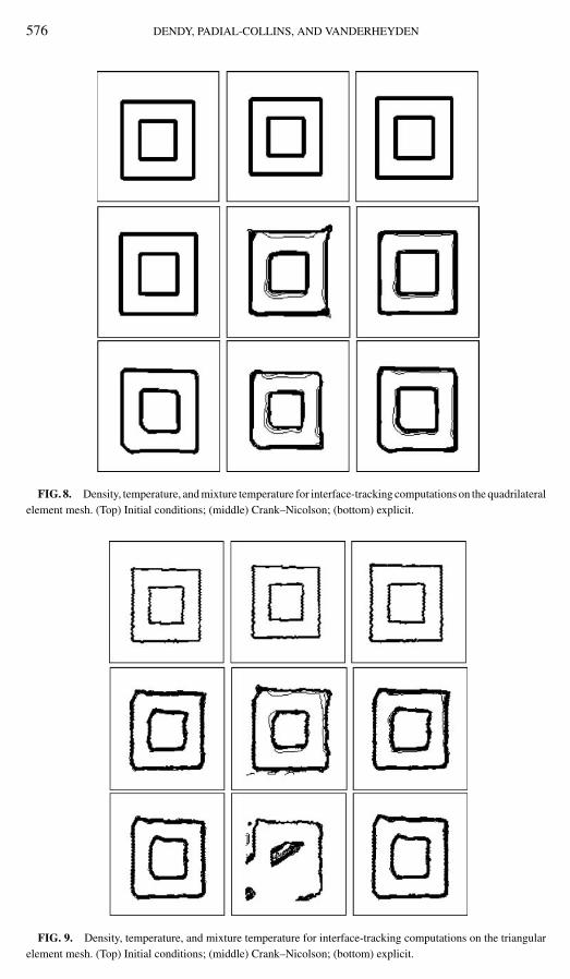
We now demonstrate the accuracy of the interface-tracking component of the new scheme.For the translation of material in a constant velocity field we start with a unit step in theshape of a hollow square for both density and temperature in the lower left corner of therectangular domain, centered at (x, y) = (0.48, 0.48). The internal width of the square is 0.4and the external width is 0.8. This is the same prescription used by Ubbink and Issa [10]. Wecompute on both the quadrilateral and triangular element meshes of the rectangular domain


FIG. 6. Continuous-field advection results demonstrating peak preservation for the mixture temperature (�q).(a) Initial condition; (b) quadrilateral element mesh results using current scheme; (c) triangular element mesh resultsusing current scheme.

discussed in Section 4. In this case we advect with a velocity field of (u, v) = (2.0, 1.0) andcompute at a Courant number of 0.25 over 750 time steps.

The results from these computations for both quadrilateral and triangular meshes areshown in Figs. 8 and 9. The “explicit” and “Crank–Nicolson” methods are as described inSection 3.4.3.

As with the continuous-field advection, we saw no noncompatible temperatures, nor anynonmonotonic density results for all cases. The shape-preservation characteristics of the ourschemes look very good as well. To quantify the accuracy of the calculation we computed

FIG. 7. Continuous-field advection results demonstrating shape presevation for the mixture temperature (�q)(a) Initial condition; (b) quadrilateral element mesh results using current scheme; (c) triangular element meshresults using current scheme.


FIG. 8. Density, temperature, and mixture temperature for interface-tracking computations on the quadrilateralelement mesh. (Top) Initial conditions; (middle) Crank–Nicolson; (bottom) explicit.

FIG. 9. Density, temperature, and mixture temperature for interface-tracking computations on the triangularelement mesh. (Top) Initial conditions; (middle) Crank–Nicolson; (bottom) explicit.


TABLE I

L1-Error Norms for the Box Translation Problem

Method L1-error norm

SLIC [6] 0.1320Hirt–Nichols [3] 0.0069FCT-VOF [7] 1.63e-8Youngs [11] 0.0258Ubbink and Issa, structured [10] 0.0250Ubbink and Issa, unstructured [10] 0.0397Present Crank–Nicolson scheme, quadrilaterals 0.0182Present Crank–Nicolson, triangles 0.0512Present explicit scheme, quadrilaterals 0.0311Present explicit scheme, triangles 0.0800

the L1-error norm of the final state as defined in [10]. Table I shows the L1-error normsas presented in [7, 10], as well as those for the current scheme for this example problem.We see that both our implicit and our explicit schemes on the quadrilateral element meshare comparable to those of Ubbink and Issa’s. Note that Rudman’s FCT–VOF and Hirtand Nichol’s method do exceedingly well for quadrilaterals. This is an artifact due to thealignment of the interface with cell faces and the one-dimensional, direction-split natureof these two schemes. As is seen in the next section the order of these errors is not typicalof these schemes for general problems. Shortcomings of our two new methods show up interms of the L1-error norms for the triangular element mesh. However, the contour plotsshow acceptable shape preservation for this problem. As in Section 4.1 it is important notto be confused by the temperature plots in Figs. 8 and 9. This pattern is expected by thedesign of our update, Eq. (11), as explained in Section 4.1.

4.3. Interface Tracking in a Vortical Shear Field

Here we perform a calculation of the deformation of a circular unit step of materialin a vortical shear field on the quadrilateral and triangular element meshes with both theC–N and explicit methods. This is a common test problem for interface tracking. In thecomputation, we advect the material with a prescribed shear velocity field for one rotation.We then reverse the velocity field and advect the material back to the original state. Theexact solution to the problem has the material returning to its original position and circularshape. The x component of velocity for the forward rotation is

u(x, y) = +sin(�x)cos(�y). (24)

The corresponding y component of velocity is

v(x, y) = −cos(�x)sin(�y). (25)

The signs of the expressions are flipped for the reverse-rotation part of the computation.The initial and final position of the material is (x, y) = (0.5, 0.2 1 + �

�) with a radius of 0.2.

We performed our computation with a time step such that the maximum Courant numberon the quadrilateral element mesh was no greater than 0.25. This corresponds to 2000


FIG. 10. Contour plot of density for interface-tracking in a vortical shear. The top row shows plots at timesof 0.0, 0.048, and 0.08 for the Crank–Nicolson scheme on the quadrilateral mesh. The bottom shows the finalresult at time 0.08 from left to right for the Crank–Nicolson interface-tracking scheme on the triangular mesh,the explicit interface-tracking scheme on the quadrilateral mesh, and the explicit interface-tracking scheme on thetriangular mesh.

total time steps. The number of time steps was retained for the triangular element meshcomputation; the maximum Courant number was 0.3. The results of the computations areshown in Fig. 10. The L1-error norms from Refs. [7, 10], along with those of our methods,are given in Table II.

As seen in the contour plots, the original circular shape is very nearly recovered in allcases. For quadrilateral element meshes the error norms reveal that our explicit methodis more accurate than all other methods, except for Young’s method. This is not whollyunexpected since the Young scheme involves considerable geometric reconstruction. Theresults on the triangular element meshes are very promising. The error norms are acceptableand no “flotsam” [7] was generated.

TABLE II

L1-Error Norms for the Vortical Shear Problem

Method L1-error norm

SLIC [6] 0.0459Hirt–Nichols [3] 0.0660FCT-VOF [7] 0.0314Youngs [11] 0.0086Ubbink and Issa, structured [10] 0.0290Ubbink and Issa, unstructured [10] 0.0182Present implicit scheme, quadrilaterals 0.0181Present implicit scheme, triangles 0.0388Present explicit scheme, quadrilaterals 0.0155Present explicit scheme, triangles 0.0346


4.4. Explicit–Implicit Advection in a Jet Flow Field

To test our explicit–implicit advection scheme a velocity field with varying Courantnumbers was necessary. In this final example, we perform a simulation of the transportof a concentration pulse in a two-dimensional jet in which the velocity decreases by 90%over the computational domain. We take our velocity field from the velocity potential for atwo-dimensional, inviscid-flow source doublet where the potential is given by

� = −

2�

cos

r,

where r, are polar coordinates and is a source strength. On the unit square, the velocitycomponents, (u, v), are

u =

2�

�2 − �2

r4

and

v =

�

��

r4,

where r2 = �2 + �2 and � and � are scaled and shifted spatial coordinates given by � =sx (x + x ) and � = sy(y + y). For our example problem, we took, x = 0.46, y = −0.5,sx = 1.0, sy = 2�( x )2, and = 1, so that u = 1 at (x, y) = (0, 0.5). The velocity field andsome corresponding streamlines are shown in Fig. 11. The coordinate (x, y) = (0, 0.5) is

FIG. 11. Velocity field and stream lines for jet flow advection problem.


noted as well. The analytical solution for the location of a particle after time (t − t0) hasbeen found to be in cylindrical coordinates

t − t0 =(

r0

sin �0

)3 �

{� − �0 + 1

2(sin 2�0 − sin 2�)

}

for the � component and

r = r0sin �

sin �0

for the radial component, where r0 and �0 are the radial and angular position of the particleat time t0. The relations

cos � = �2√�2 + �2

and

r = �

cos �,

where � and � are defined as above, are used to transform between the Cartesian andcylindrical locations of the particle.

In the example calculations, the density field was constant, and initially, the temper-ature field was zero. At time zero, the temperature of the inflowing material between(x, y) = (0, 0.45) and (x, y) = (0, 0.55) was set to one for a period of 0.5 time units, af-ter which the inflow temperature was set back to zero. Thus, a finite pulse of temperaturewas introduced into the flow. The results of the computations are shown in Fig. 12 forthe quadrilateral element mesh and Fig. 13 for the triangle element mesh. The analyticalsolution is shown by the solid lines, where the value inside the enclosed curve is one andzero elsewhere.

In the each of the figures, the top two graphics are from a simulation in which the time stepwas such that the Courant number was below one for all nodes. The bottom two graphics,on the other hand, were from computations in which the Courant number for the node at(x, y) = (0.0, 0.5) was 7.5 and decreased across the mesh to 0.075. The two graphics onthe left side of each figure show the temperature at a time of 0.5 after the initial injection.The two graphics on the right side of each figure show the temperature at a time of 5 afterthe initial injection. From the figures, we can see that the high Courant number results,which were computed using the explicit–implicit extension of our scheme, discussed inSection 3.4.4, are qualitatively similar to the fully explicit, low-Courant-number results.The most obvious discrepancy is in the early results in the left graphics, where numericalspreading is apparent. Although there are still differences at later time, the results are quitesimilar and there is no evidence of instabilities in our calculations. This similarity andstability suggests that our explicit–implicit scheme would be a useful technique to use inproblems in which localized high-velocity regions exist and computer resource constraintsprohibit a fully explicit computation. While there are inaccuracies associated with theexplicit–implicit technique, qualitatively realistic results can be obtained.


FIG. 12. Temperature contours for jet flow advection problem on quadrilateral element mesh. The solid linesare from the analytical solution.

4.5. Discussion

The motivation for the work presented in this paper was to develop an accurate general-purpose advection scheme for unstructured, as well as structured, meshes for both contin-uous and discontinuous fields. For the case of continuous-field advection, fluxed quantitiesare computed from an upstream, time-centered evaluation of the reconstructed field basedon node data and node-centered gradients. The use of our extended version of Thuburn’slimiter ensures monotonic and compatible future values of mass and mass-specific quanti-ties. This scheme has been determined to have second-order convergence on quadrilateraland triangular element meshes. For discontinuous fields, two variations of the Ubbink–Issa [10] method have been developed. The first is a fully explicit scheme that combines ourcontinuous-field face quantities with those obtained by the compressive difference scheme.These are then limited with our extended Thuburn limiter. In the second variation, we solvefor the face flux quantities using Ubbink and Issa’s Crank–Nicolson formulation but followthis with an a posteriori application of our extended version of Thuburn’s limiter insteadof their iterative correction scheme to enforce monotonicity. This ensures only one linearsolution per time step. Both methods have been shown to do quite well on both quadrilateraland triangular element meshes. Of particular note was the ability of our explicit schemeto out-perform all other methods except for Young’s method on the vortical shear flow


FIG. 13. Temperature contours for jet flow advection problem on triangular element mesh. The solid linesare from the analytical solution.

problem on quadrilateral element meshes. This is extremely promising, particularly for amethod that does not use directionally split advection nor interface reconstruction.

5. FUTURE WORK—LAGRANGIAN–EULERIAN FORMULATION

We conclude our discussion here with a look toward the use of our advection scheme ina general-purpose flow simulation code. For such a role, we must be able to use the schemein equations more complicated than Eqs. (1) and (2), specifically for the case in which theright-hand sides are not zero. For these cases, our plan is to use a Lagrangian–Eulerianintegration approach to solving the equations. Let us briefly illustrate what we mean on thegeneric equation

∂�

∂t+ ∇ · ��u = f (�), (26)

where f (�) is any Lagrangian physics, such as diffusion or pressure gradient acceleration,for example. We can apply the Lagrangian–Eulerian scheme in two steps by discretizing intime as follows. We first perform the Lagrangian step where we include the implicit flux


part of the advection operator as Aimpl,

�L =�m + �t Aimpl(�L ) + �t f (�L ). (27)

We then follow this with the Eulerian advection step

�m+1 =�L + �t Aexp l(�L ), (28)

where Aimpl(�L ) is the advection operator using only implicit flux values as defined byEq. (21) and Aexp l(�L ) is the advection operator with fluxed quantities computed usingEq. (22) and using the Lagrangian data as the known nodal data. This formulation has thedesirable property that it interpolates from a fully explicit Langrangian–Eulerian schemeto a fully implicit scheme. Thus the formulation will handle high-accuracy time-dependentproblems and steady-state problems. Moreover, the algorithm will handle problems withboth high- and low-Courant-number nodes simultaneously.

ACKNOWLEDGMENT

We gratefully acknowledge support for this work from the U.S. Department of Energy.

REFERENCES

1. P. N. Brown and Y. Saad, Hybrid Krylov methods for non-linear systems of equations, SIAM J Sci. Stat.Comput. 11, 450 (1990).

2. H. Gaskell and A. K. C. Lau, Curvature-compensated convective transport: SMART, a new boundedness-preserving transport algorithm., Int. J. Numer. Methods Fluids 8, 617 (1988).

3. C. W. Hirt and B. D. Nichols, Volume of fluid (VOF) method for the dynamics of free boundaries, J. Comput.Phys. 39, 201 (1981).

4. B. P. Leonard, Stable and accurate convective modeling procedure based on quadratic upstream interpolation,Comput. Methods Appl. Mech. Eng. 19, 59 (1979).

5. R. J. Leveque, High-resolution conservative algorithms for advection in incompressible flow, SIAM J. Numer.Anal. 33, 627 (1996).

6. W. F. Noh and P. Woodward, SLIC (Simple Line Interface Calculation), Lecture Notes in Physics (Springer-Verlag, New York, 1976), Vol. 59.

7. M. Rudman, Volume-tracking methods for interfacial flow calculations, Int. J. Numer. Methods Fluids 24,671 (1997).

8. J. Thuburn, Multidimensional flux-limited advection schemes, J. Comput. Phys. 123, 74 (1996).

9. O. Ubbink, Numerical Prediction of Two Fluid Systems with Sharp Interfaces, Ph.D. thesis (University ofLondon, 1997).

10. O. Ubbink and R. I. Issa, A method for capturing sharp interfaces on arbitrary meshes, J. Comput. Phys.153, 26 (1999).

11. D. L. Youngs, Time-dependent multi-material flow with large fluid distortion, in Numerical Methods forFluid Dynamics, edited by K. W. Morton and M. J. Baines (Academic, New York, 1982), p. 273.

a general-purpose finite-volume advection … general-purpose finite-volume advection scheme for...

Documents