a hierarchical markov model to understand the behaviour...

A Hierarchical Markov Model to Understandthe Behaviour of Agents in Business Processes

Diogo R. Ferreira1, Fernando Szimanski2, Celia Ghedini Ralha2

1 IST – Technical University of Lisbon, [email protected]

2 Universidade de Brasılia (UnB), [email protected], [email protected]

Abstract. Process mining techniques are able to discover process mod-els from event logs but there is a gap between the low-level nature ofevents and the high-level abstraction of business activities. In this workwe present a hierarchical Markov model together with mining techniquesto discover the relationship between low-level events and a high-level de-scription of the business process. This can be used to understand howagents perform activities at run-time. In a case study experiment usingan agent-based simulation platform (AOR), we show how the proposedapproach is able to discover the behaviour of agents in each activity ofa business process for which a high-level model is known.

Key words: Process Mining, Agent-Based Simulation, Markov Models,Expectation-Maximization, Agent-Object-Relationship (AOR)

1 Introduction

If one would try to understand a business process by observing people at workin an organization, the apparently chaotic nature of events would be quite con-fusing. However, if a high-level description of the business process is provided(for example, one that partitions the process into two or three main stages) thenit becomes much easier to understand the sequence of events.

Using process mining techniques [1], it is possible to analyse the low-levelevents that are recorded in information systems as people carry out their work.However, there is often a gap between the granularity of the recorded low-levelevents and the high level of abstraction at which processes are understood, doc-umented and communicated throughout an organisation. Process mining tech-niques are able to capture and analyse behaviour at the level of the recordedevents, whereas business analysts describe the process in terms of high-levelactivities, where each activity may correspond to several low-level events.

Some techniques have already been proposed to address this gap by producingmore abstract models from an event log. Basically, existing approaches can bedivided into two main groups:

2 D.R. Ferreira, F. Szimanski, C.G. Ralha

(a) Those techniques that work on the basis of models, by producing a minedmodel from the event log and then trying to create more abstract represen-tations of that model. Examples are [2] and [3].

(b) Those techniques that work on the basis of events, by translating the eventlog into a more abstract sequence of events, and then producing a minedmodel from that translated event log. Examples are [4] and [5].

In this work, we consider that the event log is produced by a number ofagents who collaborate when performing the activities in a business process.Here, an agent is understood in the sense of intelligent agent [6], and it is usedto represent a human actor in agent-based simulations. Each activity may involveseveral agents, and every time an agent performs some action, a new event isrecorded. Therefore, each activity in the process may be the origin of severalevents in the event log. The way in which agents collaborate is assumed to benon-deterministic, and process execution is assumed to be non-deterministic aswell. While the business process is described in terms of high-level activities thatare familiar to business users, the collaboration of agents at run-time is recordedin the event log as a sequence of low-level events.

In general, both the macro-level description of the business process and themicro-level sequence of events can be obtained: the first is provided by businessanalysts or process documentation, and the second can be found in event logs.However, the way in which micro-level events can be mapped to macro-levelactivities is unknown, and this is precisely what we want to find out. Given amicro-level event log and a macro-level model of the business process, our goalis to discover: (1) a micro-level model for the behaviour of agents and also (2)how this micro-level model fits into the macro-level description of the businessprocess. For this purpose, we develop a hierarchical Markov model that is ableto capture the macro-behaviour of the business process, the micro-behaviour ofagents as they work in each activity, and the relationship between the two.

2 An Example

Consider a business process that can be described on a high level as comprisingthe three main activities A, B, and C. Also, consider that three agents X, Y and Z

collaborate in order to perform each activity. In particular, activity A leads to asequence of actions by the three agents that can be represented by the sequenceof events XYZ. In a similar way, activity B leads to a sequence of events in theform YZZ(Z)..., where there may be multiple actions of agent Z until a certaincondition holds. Finally, activity C leads to a sequence of events in the form ZXY.This process is represented in Figure 1.

Executing this simple process corresponds to performing the sequence ofactivities ABC. However, in the event log we find traces such as XYZYZZZXY

without having any idea of how this sequence of events can be mapped to thesequence of activities ABC. The sequence ABC will be called the macro-sequenceand the high-level model for the business process is referred to as the macro-model. On the other hand, the sequence of events XYZYZZZXY will be called

A Hierarchical Markov Model to Understand the Behaviour of Agents 3

A B C

ZYYX Z XZ Y

Fig. 1. A simple example of a hierarchical process model

the micro-sequence and the behaviour of agents during each high-level activityis referred to as a micro-model. The problem addressed in this work is how todiscover the macro-sequence and the micro-models from a given macro-model andmicro-sequence, where these models (both macro and micro) are represented asMarkov chains.

3 Definitions

Let S be the set of possible states in a Markov chain, and let i and j be anytwo such states. Then P(j | i) is the transition probability from the currentstate i to a subsequent state j. In this work, as in [7], we extend the set S withtwo special states – a start state (◦) and an end state (•) – in order to includethe probability of the Markov chain starting and ending in certain states. Werepresent this augmented set of states as S = S∪ {◦, •}. For example, P(i | ◦) isthe probability of the Markov chain starting in state i. Similarly, P(• | i) is theprobability of the Markov chain ending in state i.

By definition, P(◦ | i) , 0,∀i∈S since nothing can come before the start state.

In the same way, P(i | •) , 0,∀i∈S since nothing can come after the end state.

Also, P(• | ◦) , 0 since the Markov chain cannot start and end immediatelywithout going through an observable state.

A Markov chain is represented by a matrix T = {pij} of transition probabil-ities, where pij = P(j | i),∀i,j∈S. More formally, a Markov chain M = 〈S,T〉 is

defined as a tuple where S is the augmented set of states and T is the transi-tion matrix between those states. The nature of the Markov chain is such that∑

j∈S P(j | i) = 1 for all states i ∈ S \ {•}. In other words, there is always somesubsequent state to the current state i, except when the end state has beenreached; in this case, we have

∑j∈S P(j | •) = 0.

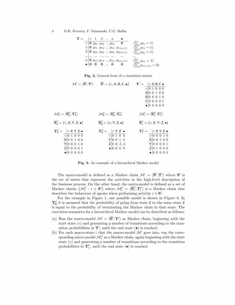
The fact that ∀j∈S : P(j | •) = 0 means that the last row in matrix T is zero.Also, the fact that ∀i∈S : P(◦ | i) = 0 means that the first column in matrix T iszero. Finally, the fact that P(• | ◦) = 0 means that the last element in the firstrow of the matrix is zero. These facts are illustrated in Figure 2.

In a hierarchical Markov model, there is a Markov chain to describe themacro-model (upper level in Figure 1), and there is a set of Markov chains todescribe the micro-model for each activity (lower level in Figure 1).


T = ◦ 1 2 ... n •◦ 0 p01 p02 ... p0n 01 0 p11 p12 ... p1n p1(n+1)

2 0 p21 p22 ... p2n p2(n+1)

... ... ... ... ... ... ...n 0 pn1 pn2 ... pnn pn(n+1)

• 0 0 0 ... 0 0

(∑

j p0j = 1)

(∑

j p1j = 1)

(∑

j p2j = 1)

...(∑

j pnj = 1)

(∑

j p(n+1)j = 0)

Fig. 2. General form of a transition matrix

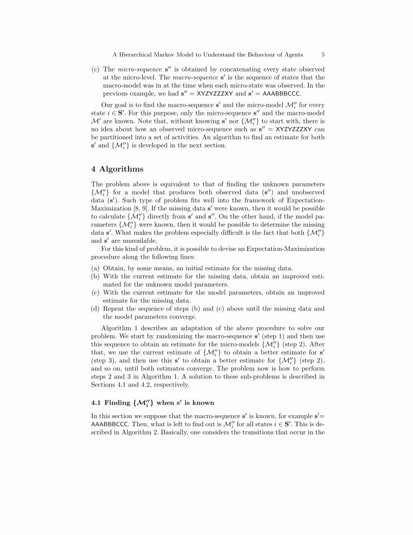
M′ = 〈S′,T′〉 S′ = {◦,A,B,C, •} T′ = ◦ A B C •◦ 0 1 0 0 0A 0 0 1 0 0B 0 0 0 1 0C 0 0 0 0 1• 0 0 0 0 0

M′′A = 〈S′′

A,T′′A〉 M′′

B = 〈S′′B,T

′′B〉 M′′

C = 〈S′′C ,T

′′C〉

S′′A = {◦,X,Y,Z, •} S′′

B = {◦,Y,Z, •} S′′C = {◦,X,Y,Z, •}

T′′A = ◦ X Y Z •

◦ 0 1 0 0 0X 0 0 1 0 0Y 0 0 0 1 0Z 0 0 0 0 1• 0 0 0 0 0

T′′B = ◦ Y Z •

◦ 0 1 0 0Y 0 0 1 0Z 0 0 .5 .5• 0 0 0 0

T′′C = ◦ X Y Z •

◦ 0 0 0 1 0X 0 0 1 0 0Y 0 0 0 0 1Z 0 1 0 0 0• 0 0 0 0 0

Fig. 3. An example of a hierarchical Markov model

The macro-model is defined as a Markov chain M′ = 〈S′,T′〉 where S′ isthe set of states that represent the activities in the high-level description ofthe business process. On the other hand, the micro-model is defined as a set ofMarkov chains {M′′

i : i ∈ S′} where M′′i = 〈S′′

i ,T′′i 〉 is a Markov chain that

describes the behaviour of agents when performing activity i ∈ S′.For the example in Figure 1, one possible model is shown in Figure 3. In

T′′B it is assumed that the probability of going from state Z to the same state Z

is equal to the probability of terminating the Markov chain in that state. Theexecution semantics for a hierarchical Markov model can be described as follows:

(a) Run the macro-model M′ = (S′,T′) as Markov chain, beginning with thestart state (◦) and generating a number of transitions according to the tran-sition probabilities in T′, until the end state (•) is reached.

(b) For each macro-state i that the macro-model M′ goes into, run the corre-sponding micro-modelM′′

i as a Markov chain, again beginning with the startstate (◦) and generating a number of transitions according to the transitionprobabilities in T′′

i , until the end state (•) is reached.


(c) The micro-sequence s′′ is obtained by concatenating every state observedat the micro-level. The macro-sequence s′ is the sequence of states that themacro-model was in at the time when each micro-state was observed. In theprevious example, we had s′′ = XYZYZZZXY and s′ = AAABBBCCC.

Our goal is to find the macro-sequence s′ and the micro-modelM′′i for every

state i ∈ S′. For this purpose, only the micro-sequence s′′ and the macro-modelM′ are known. Note that, without knowing s′ nor {M′′

i } to start with, there isno idea about how an observed micro-sequence such as s′′ = XYZYZZZXY canbe partitioned into a set of activities. An algorithm to find an estimate for boths′ and {M′′

i } is developed in the next section.

4 Algorithms

The problem above is equivalent to that of finding the unknown parameters{M′′

i } for a model that produces both observed data (s′′) and unobserveddata (s′). Such type of problem fits well into the framework of Expectation-Maximization [8, 9]. If the missing data s′ were known, then it would be possibleto calculate {M′′

i } directly from s′ and s′′. On the other hand, if the model pa-rameters {M′′

i } were known, then it would be possible to determine the missingdata s′. What makes the problem especially difficult is the fact that both {M′′

i }and s′ are unavailable.

For this kind of problem, it is possible to devise an Expectation-Maximizationprocedure along the following lines:

(a) Obtain, by some means, an initial estimate for the missing data.(b) With the current estimate for the missing data, obtain an improved esti-

mated for the unknown model parameters.(c) With the current estimate for the model parameters, obtain an improved

estimate for the missing data.(d) Repeat the sequence of steps (b) and (c) above until the missing data and

the model parameters converge.

Algorithm 1 describes an adaptation of the above procedure to solve ourproblem. We start by randomizing the macro-sequence s′ (step 1) and then usethis sequence to obtain an estimate for the micro-models {M′′

i } (step 2). Afterthat, we use the current estimate of {M′′

i } to obtain a better estimate for s′

(step 3), and then use this s′ to obtain a better estimate for {M′′i } (step 2),

and so on, until both estimates converge. The problem now is how to performsteps 2 and 3 in Algorithm 1. A solution to these sub-problems is described inSections 4.1 and 4.2, respectively.

4.1 Finding {M′′i } when s′ is known

In this section we suppose that the macro-sequence s′ is known, for example s′=AAABBBCCC. Then, what is left to find out isM′′

i for all states i ∈ S′. This is de-scribed in Algorithm 2. Basically, one considers the transitions that occur in the


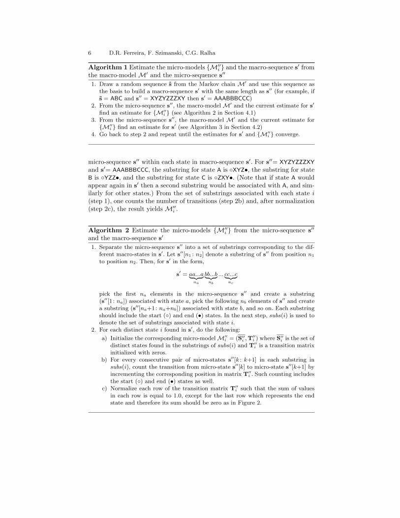
Algorithm 1 Estimate the micro-models {M′′i } and the macro-sequence s′ from

the macro-model M′ and the micro-sequence s′′

1. Draw a random sequence s from the Markov chain M′ and use this sequence asthe basis to build a macro-sequence s′ with the same length as s′′ (for example, ifs = ABC and s′′ = XYZYZZZXY then s′ = AAABBBCCC)

2. From the micro-sequence s′′, the macro-model M′ and the current estimate for s′

find an estimate for {M′′i } (see Algorithm 2 in Section 4.1)

3. From the micro-sequence s′′, the macro-model M′ and the current estimate for{M′′

i } find an estimate for s′ (see Algorithm 3 in Section 4.2)4. Go back to step 2 and repeat until the estimates for s′ and {M′′

i } converge.

micro-sequence s′′ within each state in macro-sequence s′. For s′′= XYZYZZZXY

and s′= AAABBBCCC, the substring for state A is ◦XYZ•, the substring for stateB is ◦YZZ•, and the substring for state C is ◦ZXY•. (Note that if state A wouldappear again in s′ then a second substring would be associated with A, and sim-ilarly for other states.) From the set of substrings associated with each state i(step 1), one counts the number of transitions (step 2b) and, after normalization(step 2c), the result yields M′′

i .

Algorithm 2 Estimate the micro-models {M′′i } from the micro-sequence s′′

and the macro-sequence s′

1. Separate the micro-sequence s′′ into a set of substrings corresponding to the dif-ferent macro-states in s′. Let s′′[n1 : n2] denote a substring of s′′ from position n1

to position n2. Then, for s′ in the form,

s′ = aa...a︸︷︷︸na

bb...b︸︷︷︸nb

... cc...c︸︷︷︸nc

pick the first na elements in the micro-sequence s′′ and create a substring(s′′[1 : na]) associated with state a, pick the following nb elements of s′′ and createa substring (s′′[na+1: na+nb]) associated with state b, and so on. Each substringshould include the start (◦) and end (•) states. In the next step, subs(i) is used todenote the set of substrings associated with state i.

2. For each distinct state i found in s′, do the following:

a) Initialize the corresponding micro-modelM′′i = (S′′

i ,T′′i ) where S′′

i is the set ofdistinct states found in the substrings of subs(i) and T′′

i is a transition matrixinitialized with zeros.

b) For every consecutive pair of micro-states s′′[k : k+1] in each substring insubs(i), count the transition from micro-state s′′[k] to micro-state s′′[k+1] byincrementing the corresponding position in matrix T′′

i . Such counting includesthe start (◦) and end (•) states as well.

c) Normalize each row of the transition matrix T′′i such that the sum of values

in each row is equal to 1.0, except for the last row which represents the endstate and therefore its sum should be zero as in Figure 2.


4.2 Finding s′ when {M′′i } are known

In this section, we suppose that the micro-model M′′i for each state i ∈ S′ is

available, but the macro-sequence s′ is unknown, so we want to determine s′

from s′′, {M′′i } and M′. Note that the macro-sequence s′ is produced by the

macro-modelM′, which is a Markov chain, so there may be several possibilitiesfor s′. In general, we will be interested in finding the most likely solution for s′.

The most likely s′ is given by the sequence of macro-states that is ableto produce s′′ with highest probability. In the example above, we had s′′ =XYZYZZZXY. We know that s′′ begins with X and therefore the macro-sequences′ must be initiated by a macro-state whose micro-model can begin with X. Asit happens, there is a single such macro-state in Figure 3, and it is A. So nowthat we have begun with A, we try to parse the following symbols in s′′ with themicro-model M′′

A. We find that this micro-model can account for the substringXYZ, after which it ends, so a new macro-state must be chosen to account forthe second Y in s′′.

In Figure 3, the only micro-model that begins with Y is M′′B. Therefore, the

second macro-state is B. We now use M′′B to parse the following symbols of s′′,

taking us all the way through YZZZ, when M′′B cannot parse the following X. A

third macro-state is needed to parse the final XY but no suitable solution canbe found, because the micro-model M′′

A begins with X but does not end in Y.The problem is that the parsing of micro-modelM′′

B went too far. It should havestopped on YZZ and let the final ZXY be parsed by micro-model M′′

C. In thiscase we would have s′ = AAABBBCCC.

This simple example is enough to realize that there may be the need tobacktrack and there may be several possible solutions for s′. With both s′ ands′′, together with M′ and {M′′

i }, it is possible to calculate the probability ofobserving a particular micro-sequence s′′. This is the product of all transitionprobabilities in the macro- and micro-models. Let T(i, j) denote the transitionprobability from state i to state j in a transition matrix T. Then, in the exampleabove, we have:

s′[1] = A s′′[1] = X T′(◦,A)×T′′A(◦,X) = 1.0× 1.0

s′[2] = A s′′[2] = Y T′′A(X,Y) = 1.0

s′[3] = A s′′[3] = Z T′′A(Y,Z) = 1.0

s′[4] = B s′′[4] = Y T′′A(Z, •)×T′(A,B)×T′′

B(◦,Y) = 1.0× 1.0× 1.0s′[5] = B s′′[5] = Z T′′

B(Y,Z) = 1.0s′[6] = B s′′[6] = Z T′′

B(Z,Z) = 0.5s′[7] = C s′′[7] = Z T′′

B(Z, •)×T′(B,C)×T′′C(◦,Z) = 0.5× 1.0× 1.0

s′[8] = C s′′[8] = X T′′C(Z,X) = 1.0

s′[9] = C s′′[9] = Y T′′C(X,Y)×T′′

C(Y, •)×T′(C, •) = 1.0× 1.0× 1.0

The product of all these probabilities is p = 0.25. For computational reasons,we use the log probability log(p) instead. In general, we choose the solution for s′

which yields the highest value for the log probability. The procedure is describedin Algorithm 3. In particular, step 2 in Algorithm 3 is a recursive functionthat explores all possibilities for s′ with non-zero probability. Such recursive


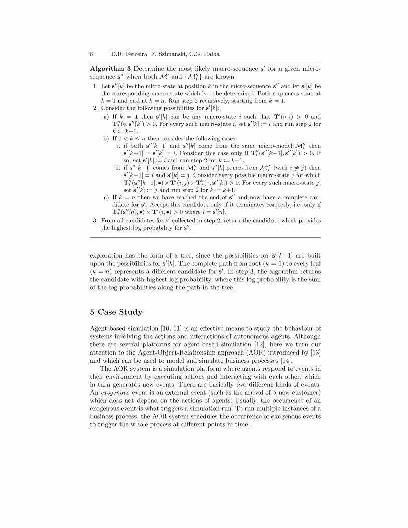
Algorithm 3 Determine the most likely macro-sequence s′ for a given micro-sequence s′′ when both M′ and {M′′

i } are known

1. Let s′′[k] be the micro-state at position k in the micro-sequence s′′ and let s′[k] bethe corresponding macro-state which is to be determined. Both sequences start atk = 1 and end at k = n. Run step 2 recursively, starting from k = 1.

2. Consider the following possibilities for s′[k]:

a) If k = 1 then s′[k] can be any macro-state i such that T′(◦, i) > 0 andT′′

i (◦, s′′[k]) > 0. For every such macro-state i, set s′[k] := i and run step 2 fork := k+1.

b) If 1 < k ≤ n then consider the following cases:i. if both s′′[k−1] and s′′[k] come from the same micro-model M′′

i thens′[k−1] = s′[k] = i. Consider this case only if T′′

i (s′′[k−1], s′′[k]) > 0. Ifso, set s′[k] := i and run step 2 for k := k+1.

ii. if s′′[k−1] comes from M′′i and s′′[k] comes from M′′

j (with i 6= j) thens′[k−1] = i and s′[k] = j. Consider every possible macro-state j for whichT′′

i (s′′[k−1], •)×T′(i, j)×T′′j (◦, s′′[k]) > 0. For every such macro-state j,

set s′[k] := j and run step 2 for k := k+1.c) If k = n then we have reached the end of s′′ and now have a complete can-

didate for s′. Accept this candidate only if it terminates correctly, i.e. only ifT′′

i (s′′[n], •)×T′(i, •) > 0 where i = s′[n].

3. From all candidates for s′ collected in step 2, return the candidate which providesthe highest log probability for s′′.

exploration has the form of a tree, since the possibilities for s′[k+1] are builtupon the possibilities for s′[k]. The complete path from root (k = 1) to every leaf(k = n) represents a different candidate for s′. In step 3, the algorithm returnsthe candidate with highest log probability, where this log probability is the sumof the log probabilities along the path in the tree.

5 Case Study

Agent-based simulation [10, 11] is an effective means to study the behaviour ofsystems involving the actions and interactions of autonomous agents. Althoughthere are several platforms for agent-based simulation [12], here we turn ourattention to the Agent-Object-Relationship approach (AOR) introduced by [13]and which can be used to model and simulate business processes [14].

The AOR system is a simulation platform where agents respond to events intheir environment by executing actions and interacting with each other, whichin turn generates new events. There are basically two different kinds of events.An exogenous event is an external event (such as the arrival of a new customer)which does not depend on the actions of agents. Usually, the occurrence of anexogenous event is what triggers a simulation run. To run multiple instances of abusiness process, the AOR system schedules the occurrence of exogenous eventsto trigger the whole process at different points in time.


The second kind of event is a message and it is the basis of simulation in theAOR system. Agents send messages to one another, which in turn generates newmessages. For example, if agent X sends a message M1 to agent Y, then this mayresult in a new message M2 being sent from Y to Z. Such chaining of messageskeeps the simulation running until there are no more messages to be exchanged.At that point, a new exogenous event is required to trigger a new simulationrun. In this work, we represent the exchange of a message M being sent from

agent X to agent Y as: XM−−−−→ Y.

Our case study is based on the implementation of a purchasing scenario inthe AOR system. On a high (macro) level, the process can be represented as inFigure 4 and can be described as follows. In a company, an employee needs acertain commodity (e.g. a printer cartridge). If the product is available at thewarehouse, then the warehouse dispatches the product to the employee. Other-wise, the product must be purchased from an external supplier. All purchasesmust be previously approved by the purchasing department. If the purchase isnot approved, the process ends immediately. If the purchase is approved, theprocess proceeds with the purchasing department ordering and paying for theproduct from the supplier. The supplier delivers the product to the warehouse,and the warehouse dispatches the product to the employee.

Fig. 4. Macro-level description of a purchase process

This process was implemented in the AOR system using the AOR SimulationLanguage (AORSL) [15] to specify the message exchanges between agents. Thereare four types of agent: Employee, Warehouse, Purchasing, and Supplier. There is oneinstance of the Warehouse agent and one instance of the Purchasing agent. However,


there are multiple instances of the Employee agent (each instance exists during asimulation run; it is created at the start of the run and destroyed when the runfinishes). We could have done the same for the Supplier agent, but for simplicitywe considered only one instance of Supplier.

The process includes the following message exchanges:

Requisition

{Employee

StockRequest−−−−−−−−−−→ Warehouse

WarehouseStockResponse−−−−−−−−−−−→ Employee

Dispatch product

Employee

FetchProduct−−−−−−−−−−→ Warehouse

WarehouseProductReady−−−−−−−−−−→ Employee

EmployeeProductReceived−−−−−−−−−−−−→ Warehouse

Approve purchase

Employee

PurchaseRequest−−−−−−−−−−−−→ Purchasing

PurchasingInfoRequest−−−−−−−−−→ Employee

EmployeeInfoResponse−−−−−−−−−−→ Purchasing

PurchasingApprovalResult−−−−−−−−−−−→ Employee

Order product

Purchasing

PurchaseOrder−−−−−−−−−−−→ Supplier

SupplierPaymentTerms−−−−−−−−−−−→ Purchasing

PurchasingPaymentVoucher−−−−−−−−−−−−→ Supplier

Receive product

{Supplier

DeliveryNote−−−−−−−−−−→ Warehouse

WarehouseProductAvailable−−−−−−−−−−−−→ Employee

It should be noted that the AOR system has no knowledge about the macro-level activities on the left-hand side. Instead, the agents have rules to implementthe message exchanges on the right-hand side. In addition, we suppose that:

– For the purchase request to be approved, the purchasing department mayenquire the employee an arbitrary number of times to obtain further infoabout the purchase request. This means that the exchanges InfoRequest andInfoResponse may occur multiple times (or even not occur at all).

– The purchasing department may not be satisfied with the payment termsrequested by a particular supplier, and may choose to negotiate those termsor get in contact with another supplier. This means that PurchaseOrder andPaymentTerms may occur multiple times (but they must occur at least once).

Simulating this process in AOR produces an event log with an AOR-specificXML structure. From this event log, it is possible to recognize each new instanceof the Employee agent as a different instance of the process. Therefore, we collectedthe sequence of events for each Employee agent; these represent our traces, i.e.the micro-sequences. The process in Figure 4 represents the macro-model, andit was converted to a Markov chain representation. Feeding the micro-sequences


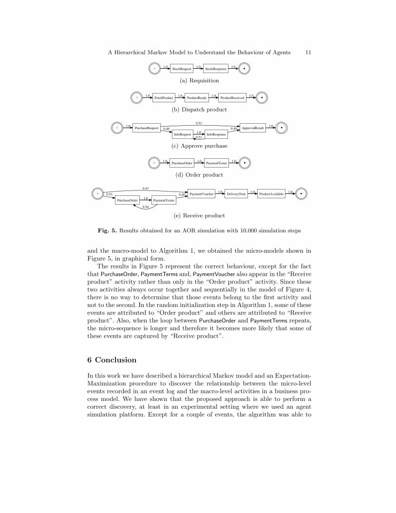
(a) Requisition

(b) Dispatch product

(c) Approve purchase

(d) Order product

(e) Receive product

Fig. 5. Results obtained for an AOR simulation with 10.000 simulation steps

and the macro-model to Algorithm 1, we obtained the micro-models shown inFigure 5, in graphical form.

The results in Figure 5 represent the correct behaviour, except for the factthat PurchaseOrder, PaymentTerms and, PaymentVoucher also appear in the “Receiveproduct” activity rather than only in the “Order product” activity. Since thesetwo activities always occur together and sequentially in the model of Figure 4,there is no way to determine that those events belong to the first activity andnot to the second. In the random initialization step in Algorithm 1, some of theseevents are attributed to “Order product” and others are attributed to “Receiveproduct”. Also, when the loop between PurchaseOrder and PaymentTerms repeats,the micro-sequence is longer and therefore it becomes more likely that some ofthese events are captured by “Receive product”.

6 Conclusion

In this work we have described a hierarchical Markov model and an Expectation-Maximization procedure to discover the relationship between the micro-levelevents recorded in an event log and the macro-level activities in a business pro-cess model. We have shown that the proposed approach is able to perform acorrect discovery, at least in an experimental setting where we used an agentsimulation platform. Except for a couple of events, the algorithm was able to


associate the micro-events with the correct macro-activity, while also providinga micro-model for the behaviour of agents in each of those activities. In futurework, we will be looking into the problems that arise when applying the approachto real-world event logs with noise. The approach can be applied in scenarioswhere a macro-level description of the business process is available.

References

1. van der Aalst, W.M.P.: Process Mining: Discovery, Conformance and Enhancementof Business Processes. Springer (2011)

2. Greco, G., Guzzo, A., Pontieri, L.: Mining hierarchies of models: From abstractviews to concrete specifications. In: 3rd International Conference on BusinessProcess Management. Volume 3649 of LNCS. Springer (2005) 32–47

3. Gunther, C.W., van der Aalst, W.M.P.: Fuzzy mining – adaptive process simpli-fication based on multi-perspective metrics. In: 5th International Conference onBusiness Process Management. Volume 4714 of LNCS. Springer (2007) 328–343

4. Gunther, C.W., Rozinat, A., van der Aalst, W.M.P.: Activity mining by globaltrace segmentation. In: BPM 2009 International Workshops. Volume 43 of LNBIP.Springer (2010) 128–139

5. Bose, R.P.J.C., Verbeek, E.H.M.W., van der Aalst, W.M.P.: Discovering hierar-chical process models using ProM. In: CAiSE Forum 2011. Volume 107 of LNBIP.Springer (2012) 33–48

6. Wooldridge, M., Jennings, N.R.: Intelligent agents: Theory and practice. Knowl-edge Engineering Review 10(2) (1995) 115–152

7. Veiga, G.M., Ferreira, D.R.: Understanding spaghetti models with sequence clus-tering for ProM. In: BPM 2009 International Workshops. Volume 43 of LNBIP.Springer (2010) 92–103

8. Dempster, A.P., Laird, N.M., Rubin, D.B.: Maximum likelihood from incompletedata via the EM algorithm. Journal of the Royal Statistical Society 39(1) (1977)1–38

9. McLachlan, G.J., Krishnan, T.: The EM Algorithm and Extensions. Wiley Seriesin Probability and Statistics. Wiley-Interscience (2008)

10. Bonabeau, E.: Agent-based modeling: Methods and techniques for simulating hu-man systems. PNAS 99(Suppl 3) (2002) 7280–7287

11. Davidsson, P., Holmgren, J., Kyhlback, H., Mengistu, D., Persson, M.: Applicationsof agent based simulation. In: 7th International Workshop on Multi-Agent-BasedSimulation. Volume 4442 of LNCS. Springer (2007)

12. Railsback, S.F., Lytinen, S.L., Jackson, S.K.: Agent-based simulation platforms:Review and development recommendations. Simulation 82(9) (2006) 609–623

13. Wagner, G.: AOR modelling and simulation: Towards a general architecture foragent-based discrete event simulation. In: 5th International Bi-Conference Work-shop on Agent-Oriented Information Systems. Volume 3030 of LNCS. Springer(2004) 174–188

14. Wagner, G., Nicolae, O., Werner, J.: Extending discrete event simulation by addingan activity concept for business process modeling and simulation. In: Proceedingsof the 2009 Winter Simulation Conference. (2009) 2951–2962

15. Nicolae, O., Wagner, G., Werner, J.: Towards an executable semantics for activitiesusing discrete event simulation. In: BPM 2009 International Workshops. Volume 43of LNBIP. Springer (2010) 369–380

a hierarchical markov model to understand the behaviour...

Documents