Duquesne University • 1-19Draft IV

Duquesne University

Bayesian Hierarchical ModelsResearch and Development

Steve Bronder1∗,

1 Department of Economics, Duquesne University, 600 Forbes Avenue, 15282, Pittsburgh, PA

Abstract: The problem with marketing data is that it is characterized by many ’units’ of analysis (many respondents,households, customers), with just a few observations each. Desire for heterogeneity among respondent pre-dictions causes a challenge. The purpose of this documentation is to present a practical understanding andimplimentation of a Bayesian Hierarchical model. Bayesian Hierarchical models allow analysts to accountfor endogeneity. A Bayesian Hierarchical model is a Bayesian network, a probabilistic graphical model thatrepresents a set of random variables and their conditional dependencies via a directed acyclic graph . BayesianHierarchical models subset themselves by containing three or more levels of random variables or use latentvariables. One level uses within-unit analysis and another level for across-unit analysis. Within-unit model de-scribes individual respondents over time. Across-unit analysis is used to describe the diversity, or heterogeneity,of the units.

MSC: 62C10, 62-01

Keywords: Bayesian • MCMC • Hierarchical© For use with Demand Elasticity Research

12

1. Introduction

The problem with marketing data is that it is characterized by many ’units’ of analysis (many respondents,

households, customers), with just a few observations each. Desire for heterogeneity among respondent predictions

causes a challenge. The purpose of this documentation is to present a practical understanding and implimentation

of a Bayesian Hierarchical model. Bayesian Hierarchical models allow analysts to account for endogeneity. A

Bayesian Hierarchical model is a Bayesian network, a probabilistic graphical model that represents a set of

random variables and their conditional dependencies via a directed acyclic graph . Bayesian Hierarchical models

contain three or more levels of random variables or use latent variables. One level uses within-unit analysis and

another level for across-unit analysis. Within-unit model describes individual respondents over time. Across-unit

analysis is used to describe the diversity, or heterogeneity, of the units.

∗ E-mail: Bronder1@duq.edu

1

Bayesian Hierarchical Models

2. Framework

Suppose we measure price sensitivity with the following model where yt is dependent on an intercept β0, coefficient

β1, and error that is distributed (∼) by a normal distribution (N) with mean zero and variance σ2:

yt = β0 + β1pricet + ε ; ε ∼ Normal(0, σ2) (1)

Given the price at any time, t, one can compute β0 +β1pricet and find the expected demand yt. the parameter σ2

measures the variance of the error term. Large variances mean less accurate predictions and if variances are not

constant you break the homoskedastic assumption of least squares methods. This problem of heteroskedasticity

in marketing data forces a censored approach such that

yt =

1 ⇐⇒ β0 + β1pricet + ε > 0

0 ⇐⇒ β0 + β1pricet + ε < 0(2)

Models like equation 2 allow market researchers to quantify expected demand rather than use qualitative methods

such as crosstabs and graphics.

2.1. Hierarchical Bayes

Consider equation 2 where demand is distributed by a censored realization of an underlying continuous process.

The censoring mechanism can be written as a hierarchical model by introducing a latent variable1, zt.

yt =

1 ⇐⇒ zt > 0

0 ⇐⇒ zt < 0zt = β0 + β1pricet + εt ; εt ∼ Normal(0, σ2) (3)

Note that the latent variable allows us to make inferences about β0, β1, and σ2 that are independent of yt given

zt.

Equation 3 Examples

• A purchased is made (yt = 1) if the value of an offering is sufficiently large (Zt = 0)

• Data from multiple respondents modeled with equations 3 and 4.

– distribution of coefficients (β0, β1) distributed in the population according to a distribution whose

parameters can be estimated

– e.g. bivariate normal distribution explained by random-effects model

1 A latent variable is simply a made up variable that concactenates the hierarchical model

2

S. Bronder

Uses for Hierarchical Models

In marketing, hierarchical models are used to describe:

1. The behavior of a specific respondents in a study (within-unit behavior)

2. The distribution of responses among respondents (cross-sectional variation in parameters) 2

3. Bayesian Analysis

Bayesian methods are based on the assumption that probability is operationalized as a degree of belief, and not

a frequency such as is in classical or frequentist statistics. This is built on the idea that even though the data

given to us is a fixed time frame, the possibility of other realizations of the data have to be included. Without

observing the multiple realizations of the data required to construct measures of uncertainty we cannot be sure

of the true value of the expected variability of the statistic.

3.1. Bayes Theorem

Bayes theorem gives the ability to reverse conditionality from Pr(T |H) to Pr(H|T ) by taking the posterior odds

and making them equal to a likelihood ratio times prior odds. Equation seven comes from an example heart test.

the expression on the left hand side is the posterior odds of a heart attack given a positive test result, the first

factor on the right hand side is the likelihood ratio, and the second factor on the right is the prior odds.

Pr(H + |T+)Pr(H − |T+) = Pr(T + |H+)

Pr(T + |H−) ×Pr(H+)Pr(H−) (4)

Bayes theorem moves away from the likelihood, which conditions on presence of the disease, to a statistic that

is relevant and allows the updating of prior beliefs. The numerator of the likelihood ratio is the sensitivity of

the laboratory test, and the denominator is equal to one minus the specificity. Due to computational constraints

until the last decade bayesian models were unpopular. Recently however, statistical packages have been given the

ability to calculate these conditionals much quicker.Another way to write bayesian models is to say the posterior

is proportional3 to the likelihood times prior, or:

Posterior α Likelihood× Prior (5)

2 This is also called the distribution of heterogeneity3 The posterior is proportional because Pr(T+) does not cancel out

3

Bayesian Hierarchical Models

4. MCMC Methods

Monte Carlo Markov Chain methods work to randomly sample from the supposed marginal distribution. MCMC

methods substitute a set of repetitive calculations that, in effect, simulate draws from each variables marginal

distribution. These Monte Carlo draws can then be used to calculate statistics of interest such as parameter

estimates and confidence intervals. MCMC works like this:

1. Draw β given the data Y = yt, xt and the most recent draw of σ2

2. Draw σ2 given the data Y = yt, xt and the most recent draw of β

3. repeat

and the Markov chain for the model described by equations 1.3 and 1.4 are:

1. Draw zt given the data yt, xt and most recent draws of other model parameters

2. Draw β0 given zt and most recent draws of other model parameters

3. Draw β1 given zt and most recent draws of other model parameters

An advantage of estimating hierarchical bayes models with Markov Chain Monte Carlo methods is that it yields

estimates of all model parameters, including estimates of model parameters associated with specific respondents.

In addition, the use of simulation-based estimation methods, such as MCM, facilitate the study of functions of

model parameters that are closely related to decisions faced by management. In short, MCMC allows us to

analyze extreme cases. Cases in which people highly value a new product or lowly value their current product.

5. Interpreting MCMC R code

This section will use the packages MCMCpack and coda to perform a Bayesian hierarchical regression. The

function MCMChregress() simulates from the posterior distribution sample using the blocked Gibbs sampler of

Chib and Carlin (1999), Algorithm 2. MCMCpack was compiled in optimized C++ code to maximize efficieny,

leading to much faster resampling times relative to packages such as bayesm.

The model takes the following form:

yi = Xiβ +Wibi + εi (6)

Where each group i have ki observations.

Where the random effects:

bi ∼ Np(0, Vb) (7)

4

S. Bronder

And the errors:

ε ∼ N(0, σ2Iki ) (8)

Assume standard, conjugate priors:

β ∼ Np(µβ , Vβ) (9)

And:

σ2 ∼ IGamma(v, 1/ζ) (10)

And:

Vb ∼ IWishart(r, rR) (11)

In summary, the function MCMChregress is a random and fixed effects model. The random effects are distributed

by an inverse wishart distribution and the fixed effects are distributed by an inverse gamma distribution4. The

inverse gamma distribution allows the fixed effects prior to be uninformative. The Inverse-Wishart distribution

is the multivariate extension of the inverse chi-square. In the above, rR is a covariance matrix with r degrees of

freedom. The output can be though of as a covariance matrix, or a precision matrix.

We will first start with a modified example from the MCMCpack vignette. We will generate some random

correlated data, place it in a dataframe,and perform an MCMC hierarchical regression. Simple summary tables

and graphs will be pulled for analysis and convergence testing. To perform this example download the pacakges

ggplot2, MCMCpack, coda, and nlme.

# ==========================================# Hierarchical Gaussian Linear

# Regression # ==========================================#

library(ggplot2)

library(MCMCpack)

library(nlme)

# ===============# Generating Data# ===============#

4 While the error term is actually distributed by the inverse gamma the prior selection for this distribution changethe outcome of the fixed effects model.

5

Bayesian Hierarchical Models

# Constants

nobs <- 1000

nspecies <- 20

# Groups

species <- c(1:nspecies, sample(c(1:nspecies), nobs - nspecies, replace = TRUE))

# Covariates

X1 <- runif(n = nobs, min = 0, max = 10)

X2 <- runif(n = nobs, min = 0, max = 10)

X <- cbind(rep(1, nobs), X1, X2)

W <- X

# Target parameters beta

beta.target <- matrix(c(0.1, 0.3, 0.2), ncol = 1)

# Vb

Vb.target <- c(0.5, 0.2, 0.1)

# b

b.target <- cbind(rnorm(nspecies, mean = 0, sd = sqrt(Vb.target[1])), rnorm(nspecies,

mean = 0, sd = sqrt(Vb.target[2])), rnorm(nspecies, mean = 0, sd = sqrt(Vb.target[3])))

# sigma2

sigma2.target <- 0.02

# Response

Y <- vector()

for (n in 1:nobs) {

Y[n] <- rnorm(n = 1, mean = X[n, ] %*% beta.target + W[n, ] %*% b.target[species[n],

6

S. Bronder

], sd = sqrt(sigma2.target))

}

# Data-set

Data <- as.data.frame(cbind(Y, X1, X2, species))

qplot(X1, Y, data = Data, colour = species, size = X2)

0

5

10

15

0.0 2.5 5.0 7.5 10.0X1

Y

X2

2.5

5.0

7.5

5

10

15

20species

The above code is used to generate groups, independent variables and the dependent variable5. The dataset is

comprised of two dependent variables, a group of species catagorized from 1 to 20, and a dependent variable that

is our target. Our next step is to specify a prior.

To perform a hierarchical analysis we have to create two models. One model will contain the fixed effects, the

effects that cause shifts in the intercept term. The other model will contain the random effects, the effects

that allows each species to take on a different shape. The two variables in this example have been purposely

built to model random and fixed effects in one equation. A general rule of thumb is to establish priors based

off of a frequentist model. This example will use the function lme() from the package nlme to estimate a

5 The group is called species. X1 and X2 are independent variables. Y is the dependent. For questions aboutspecific functions in the section above use ?function

7

Bayesian Hierarchical Models

linear mixed effect model based on restricted maximum likelyhood. The first parameter of the linear mixed

effect model is the fixed effects written in standard formula syntax. On the left is the dependent variable with

independent variables to the right. Notice the zero in the formula specifies no intercept is to be included. The

data parameter specifies the object that contains our data. The next parameter is the random effect model

we wisht to specify. In this section only the right hand side is filled with independent variables. After the

random effect variables are specified use the | to name the column containing the factors describing your hierarchy.6

To establish a prior for the Bayesian Hierarchical model take the covariance variance matrix of the random effects

as the scale matrix for the inverse wishart distribution. Repeatedly sample from the wishart distribution with

the function rrgrab(). This function takes the iterates over the inverse wishart and aggregates an array into

the means of x samples. The variable df represents the degrees of freedom when pulling from the Wishart. As

a general rule of thumb, a higher confidence in a prior, the higher the degrees of freedom. We save memory by

using the function rm() to remove objects z and a from the enviroment.

prior.lm <- lme(Y ˜ X1 + X2 + 0, data = Data, ˜X1 + X2 | species)

prior.cov <- getVarCov(prior.lm)

rrgrab <- function(x, samp, samples = NULL, df = NULL) {

for (i in 1:samp) {

samples[[i]] <- rwish(df, x)

}

a <- simplify2array(samples)

b <- apply(a, c(1, 2), mean)

6 It’s essential to understand the why and when to use mixed models and what type of mixed model you need.Please read ”Mixed Effect Models in S and S-PLUS” for an in depth discussion on building linear and nonlinearmixed models.

8

S. Bronder

return(b)

}

z <- rrgrab(prior.cov, samp = 10000, df = 1000)

a <- rrgrab(prior.cov, samp = 10000, df = 1000)

bb <- (z + a)/2

rm(z)

rm(a)

6. MCMChregress Function

The next section will perform the MCMChregress and generate plots to measure prediction. MCMChregress(),

from the package MCMCpack performs the Bayesian Hierarchical model. Fixed is our fixed effects model written

in standard formula syntax. On the left is our dependent variable and on the right is our independent variable.

Random contains our random effects model, or the model we use to estimate our group differences. Notice this

is also written in standard formula syntax, but because a latent variable is predicted here we leave the left side

of the tilde blank. Group will contain the name of the column which holds the factors the random effects model

is used on. Data specifies your dataset, burnin is the number of iterations to perform before the sampling of the

MCMC starts. The mcmc parameter specifies how many iterations the function will pull values from. In the

code below, thin tells the function to only take one out of every five of the mcmc iterations as values. Thinning

helps to improve the odds that our final MCMC chain will be stationary. Verbose can be set to 1 or 0. If 1, the

function will output where it is in the resampling process. seed is used to specify which random number bank to

start with. NA in seed will use seed = (1234), the default seed.

The rest of the parameters are all for specifying our priors for the random and fixed effects. If set to NA,

beta.start and sigma2.start will use the OLS regression betas and residual error variance, respectively. beta.start

can also accept a scalar or custom vector. Vb.start contains starting values for variance matrix of the random

effects. This must be a qxq dimension matrix where q is the number of coefficients7. Default value of NA uses

7 including the intercept

9

Bayesian Hierarchical Models

an identity matrix. mubeta and Vbeta are the mean and variance of the fixed effect coefficients. You can use

random samplings like above, but for an inverse gaussian distribution to receive the mean and variance. Leave

these as 0 and 1 for a less informative prior. For an uninformative prior, set r equal to q. The parameter r is the

shape parameter for the Inverse-Wishart prior on variance matrix for the random effects. r must be superior or

equal to q. R is the scale matrix for the Inverse-Wishart prior on variance matrix for the random effects. This

must be a square q-dimension matrix. For R use the term bb we found from the inverse wishart sampling. nu and

delta specify the shape and rate parameter for the inverse gamma prior for the residual error variance. Leaving

these out or setting them each to .001 will give you an uninformative prior.

# =====================# Call to MCMChregress# =====================#

model <- MCMChregress(fixed = Y ˜ X1 + X2, random = ˜X1 + X2, group = "species",

data = Data, burnin = 30000, mcmc = 20000, thin = 5, verbose = 0, seed = NA,

beta.start = 0, sigma2.start = 1, Vb.start = prior.cov, mubeta = 0, Vbeta = 1e+06,

r = 3, R = bb, nu = 0.001, delta = 0.001)

##

## Running the Gibbs sampler. It may be long, keep cool :)

a <- Data$Y - model$Y.pred

StateplotError <- qplot(a, colour = species, data = Data, xlab = "Error", ylab = "Count",

geom = "density", size = X1) + guides(colour = guide_legend(ncol = 2))

Stateplot <- qplot(model$Y.pred, Y, colour = species, data = Data, xlab = "Bayesian Prediction",

ylab = "True Value of Y", size = X2) + guides(colour = guide_legend(ncol = 2))

a <- Data$Y - model$Y.pred

StatebyplotError <- qplot(a, colour = species, data = Data, facets = ˜species,

xlab = "Error", ylab = "Count", geom = "density", size = X1) + guides(colour = guide_legend(ncol = 2))

Statebyplot <- qplot(model$Y.pred, Y, colour = species, facets = ˜species, data = Data,

xlab = "Bayesian Prediction", ylab = "True Value of Y") + guides(colour = guide_legend(ncol = 2))

StateplotError

10

S. Bronder

0

1

2

3

−0.25 0.00 0.25Error

Cou

nt

Stateplot

0

5

10

15

0 5 10 15Bayesian Prediction

True

Val

ue o

f Y

X2

2.5

5.0

7.5

species

5

10

15

20

11

Bayesian Hierarchical Models

StatebyplotError

1 2 3 4 5

6 7 8 9 10

11 12 13 14 15

16 17 18 19 20

0

1

2

3

0

1

2

3

0

1

2

3

0

1

2

3

−0.250.00 0.25 −0.250.00 0.25 −0.250.00 0.25 −0.250.00 0.25 −0.250.00 0.25Error

Cou

nt

species

5

10

15

20

Statebyplot

1 2 3 4 5

6 7 8 9 10

11 12 13 14 15

16 17 18 19 20

05

1015

05

1015

05

1015

05

1015

0 5 10 15 0 5 10 15 0 5 10 15 0 5 10 15 0 5 10 15Bayesian Prediction

True

Val

ue o

f Y

species

5

10

15

20

12

S. Bronder

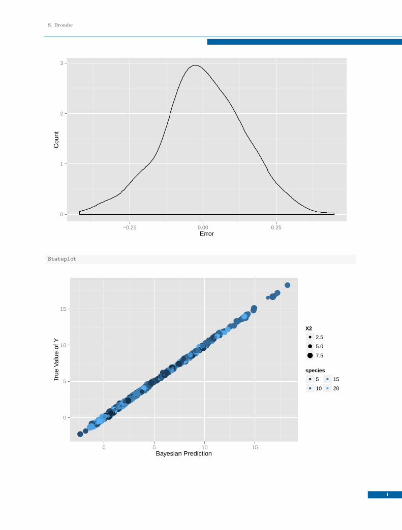
The plots above makes a rough visual examination of the model possible. The graphs plot density distributions

of the error terms, model prediction versus real Y values, the densities of the error term for each species, and

the model prediction versus real Y values for each species. The predicted Y values are already generated by the

model list as Y.pred.

7. Model Evaluation

7.1. Convergence

To check convergence of the markov chain we use the functions in the coda package. In the example below plots

are made to check the autocorrelation, cross-correlation, and the Geweke convergence diagnostic. Consider an

MCMC that is strongly autocorrelated. Autocorrelation produces clumpy samples that are unrepresentative of

the true underlying posterior distributions. Thinning the sample helps reduce the autocorrelation, but it is still

important to examine autocorrelation plots and diagnostics.

When performing a summary on the chain you will receive the mean, standard deviation, naive standard

deviation, and time series adjusted standard deviation. This is the go-to diagnostic and end result for most users.

However, it is necessary to know that these numbers are generated under the assumption that each variable

is ”marginalized”, i.e. other parameters having any values according to their posterior probabilities. If some

variables are correlated with one another than parameter uncertainties appear much greater in the marginals

than they actually are. Making a plot of the cross-correlations allows examination of the pair-wise correlation.

Its important to be careful when simply taking the mean and standard deviation of the chains as this is not what

the analysis is built for8

The last plot in this set of convergence tests is the Geweke diagnostic. The Geweke diagnostic takes two nonover-

lapping parts of the chain, usually near the beginning and end, and comparest the means of both parts. This test

attempts to reveal whether the whole chain has converged by performing a z-test on the means with standard

errors adjusted for autocorrelation. Failing this test implies the entirety of the chain has not converge and the

lowest 10 percent should be cut off. This is repeated until convergence is satisfied or only 50 percent of the chain

remains. At the 50 percent mark the chain is considered a failure. The plots below perform this process for the

chain. As long as your marks stay mostly inside of the dotted line your chain is considered sufficient.

8 In fact, for models where that is the main interest the lme function would suffice.

13

Bayesian Hierarchical Models

autocorr.plot(model$mcmc[, 1:3])

0 50 100 150

−1.

00.

01.

0

Lag

Aut

ocor

rela

tion

beta.(Intercept)

0 50 100 150

−1.

00.

01.

0

Lag

Aut

ocor

rela

tion

beta.X1

0 50 100 150

−1.

00.

01.

0

Lag

Aut

ocor

rela

tion

beta.X2

crosscorr.plot(model$mcmc)

bt.(In) b.(I).3 b.X1.19 b.X2.17 sigma2

Dev

ianc

b.X

2.2

b.X

1.5

b.(I

).9

b.(I

).12 1

−1

0

14

S. Bronder

geweke.plot(model$mcmc[, 1:2])

30000 34000 38000

−2

−1

01

2

First iteration in segment

Z−

scor

e

beta.(Intercept)

30000 34000 38000

−2

−1

01

2

First iteration in segment

Z−

scor

e

beta.X1

7.2. Summary Evaluation

After testing for convergence the chain can be evaluated. However, keep in mind the limitations in interpretation

due to possible cross-correlation. The following code outputs the summary statistics, plots the marginal density

and trace plots, and outputs the credible intervals9. After noticing the cross-correlation we can look at our mean

and time series standard errors knowing there may be a bias in shrinking the numbers down to single terms.

summary(model$mcmc[, 1:6])

##

## Iterations = 30001:49996

## Thinning interval = 5

## Number of chains = 1

## Sample size per chain = 4000

##

9 removing the [,1:n] in each function will give all of the output. To save space only a portion of it is retrievedhere.

15

Bayesian Hierarchical Models

## 1. Empirical mean and standard deviation for each variable,

## plus standard error of the mean:

##

## Mean SD Naive SE Time-series SE

## beta.(Intercept) 0.319 0.286 0.00452 0.00452

## beta.X1 0.466 0.175 0.00276 0.00276

## beta.X2 0.259 0.144 0.00228 0.00234

## b.(Intercept).1 0.509 0.292 0.00462 0.00462

## b.(Intercept).10 0.233 0.290 0.00458 0.00458

## b.(Intercept).11 0.993 0.294 0.00465 0.00465

##

## 2. Quantiles for each variable:

##

## 2.5% 25% 50% 75% 97.5%

## beta.(Intercept) -0.2538 0.1378 0.318 0.500 0.884

## beta.X1 0.1208 0.3546 0.464 0.580 0.816

## beta.X2 -0.0186 0.1625 0.257 0.353 0.555

## b.(Intercept).1 -0.0689 0.3252 0.507 0.696 1.091

## b.(Intercept).10 -0.3460 0.0546 0.235 0.418 0.807

## b.(Intercept).11 0.4140 0.8054 0.991 1.184 1.578

plot(model$mcmc[, 1:3])

16

S. Bronder

30000 35000 40000 45000 50000

−0.

51.

0

Iterations

Trace of beta.(Intercept)

−1.0 −0.5 0.0 0.5 1.0 1.5

0.0

1.0

Density of beta.(Intercept)

N = 4000 Bandwidth = 0.0546

30000 35000 40000 45000 50000

0.0

1.0

Iterations

Trace of beta.X1

0.0 0.5 1.0

0.0

1.5

Density of beta.X1

N = 4000 Bandwidth = 0.03398

30000 35000 40000 45000 50000

−0.

40.

6

Iterations

Trace of beta.X2

−0.5 0.0 0.5 1.0

0.0

2.0

Density of beta.X2

N = 4000 Bandwidth = 0.02873

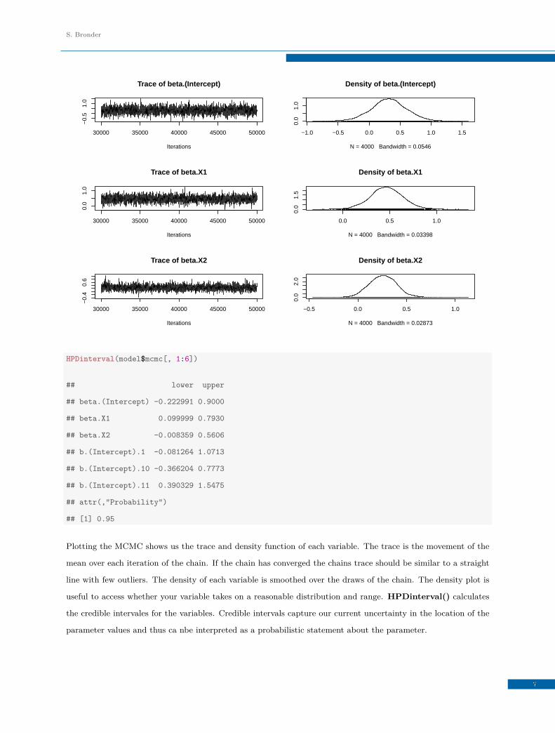
HPDinterval(model$mcmc[, 1:6])

## lower upper

## beta.(Intercept) -0.222991 0.9000

## beta.X1 0.099999 0.7930

## beta.X2 -0.008359 0.5606

## b.(Intercept).1 -0.081264 1.0713

## b.(Intercept).10 -0.366204 0.7773

## b.(Intercept).11 0.390329 1.5475

## attr(,"Probability")

## [1] 0.95

Plotting the MCMC shows us the trace and density function of each variable. The trace is the movement of the

mean over each iteration of the chain. If the chain has converged the chains trace should be similar to a straight

line with few outliers. The density of each variable is smoothed over the draws of the chain. The density plot is

useful to access whether your variable takes on a reasonable distribution and range. HPDinterval() calculates

the credible intervales for the variables. Credible intervals capture our current uncertainty in the location of the

parameter values and thus ca nbe interpreted as a probabilistic statement about the parameter.

17

Bayesian Hierarchical Models

8. Conclusion

The purpose of this documentation is to present a practical understanding and implimentation of a Bayesian

Hierarchical model. Bayesian Hierarchical models allow analysts to account for endogeneity. A Bayesian

Hierarchical model is a Bayesian network, a probabilistic graphical model that represents a set of random

variables and their conditional dependencies via a directed acyclic graph . Bayesian Hierarchical models contain

three or more levels of random variables or use latent variables. One level uses within-unit analysis and another

level for across-unit analysis. Within-unit model describes individual respondents over time. Across-unit analysis

is used to describe the diversity, or heterogeneity, of the units.

The rule of thumb when choosing between a Bayesian or Frequentist model is this. A good Frequentist model is

much better than a bad Bayesian model, but a good Bayesian model will be better than a good Frequentist model.

The ability to impliment priors in the likelihood function creates the opportunity for a statistician to impose their

bias on the model. Priors for hierarchical models most certainly matter. A bias in the wrong direction could

easily sway research towards the wrong conclusion. Further research could focus on mixed model formulation,

hierarchical structure identification, and satisfactory convergence criterion. Packages also exist for R that allow

parallel computation MCMC methods on GPUs. Parallel processing of chains increases speed dramatically.

18

S. Bronder

References

[1] Steven W. Nydick,The Wishart and Inverse Wishart Distributions, In: http://www.tc.umn.edu/˜nydic001/

docs/unpubs/Wishart_Distribution.pdf, May 25th, 2012

[2] Craigmile, Peter. ”Hierarchical Model Building, Fitting, and Checking: A Behind-the-Scenes Look at a

Bayesian Analysis of Arsenic Exposure Pathways.” Bayesian Analysis 4 (2009): 1-36. Print.

[3] Martin, Andrew , Kevin Quinn, and Jong Hee Park. ”MCMCpack: Markov Chain Monte Carlo in R.” Journal

of Statistical Software 42.9 (2011): 1-16. Jstatsoft.org. Web. 21 July 2014.

[4] Resnik, Philip , and Eric Hardisty. ”Gibbs Sampling for the Uninitiated.” Umd.edu. N.p., n.d. Web. 21 July

2014. ¡http://www.umiacs.umd.edu/ resnik/pubs/gibbs.pdf¿.

[5] Draper, David . Bayesian hierarchical Modeling. Santa Cruz: Department of Applied Statistics University of

California, Santa Cruz, 2001. Print.

[6] Rossi, Peter E., Greg M. Allenby, and Robert E. McCulloch. Bayesian statistics and marketing. Hoboken,

NJ: Wiley, 2005. Print.

[7] R Core Team (2014). R: A language and environment for statistical computing. R Foundation for Statisti-

calComputing, Vienna, Austria. URL http://www.R-project.org/.

[8] Andrew D. Martin, Kevin M. Quinn, Jong Hee Park (2011). MCMCpack: Markov Chain Monte Carlo in R.

Journal of Statistical Software. 42(9): 1-21. URL http://www.jstatsoft.org/v42/i09/.

[9] Peter Rossi. (2012). bayesm: Bayesian Inference for Marketing/Micro-econometrics. R package version 2.2-5.

http://CRAN.R-project.org/package=bayesm

[10] H. Wickham. ggplot2: elegant graphics for data analysis. Springer New York, 2009.

[11] Pinheiro, Jose , and Douglas Bates. Mixed Effect Models in S and S-PLUS. New York: Springer, 2000. Print.

[12] Pinheiro J, Bates D, DebRoy S, Sarkar D and R Core Team (2014). nlme: Linear and Nonlinear Mixed

Effects Models. R package version 3.1-117.

[13] Martyn Plummer, Nicky Best, Kate Cowles and Karen Vines (2006). CODA: Convergence Diagnosis and

Output Analysis for MCMC, R News, vol 6, 7-11.

[14] Cowles, Mary Kathryn, and Bradley P. Carlin. ”Markov Chain Monte Carlo Convergence Diagnostics: A

Comparative Review.” Journal of the American Statistical Association 91.434 (1996): 883. Print.

19