a geophysical delineation of a normal fault within the
TRANSCRIPT

Stephen F. Austin State University Stephen F. Austin State University
SFA ScholarWorks SFA ScholarWorks
Electronic Theses and Dissertations
5-12-2018
A Geophysical Delineation of A Normal Fault Within the Gulf A Geophysical Delineation of A Normal Fault Within the Gulf
Coastal Plain, Montgomery County, Texas Coastal Plain, Montgomery County, Texas
Danielle Minteer [email protected]
Follow this and additional works at: https://scholarworks.sfasu.edu/etds
Part of the Geology Commons, and the Geophysics and Seismology Commons
Tell us how this article helped you.
Repository Citation Repository Citation Minteer, Danielle, "A Geophysical Delineation of A Normal Fault Within the Gulf Coastal Plain, Montgomery County, Texas" (2018). Electronic Theses and Dissertations. 153. https://scholarworks.sfasu.edu/etds/153
This Thesis is brought to you for free and open access by SFA ScholarWorks. It has been accepted for inclusion in Electronic Theses and Dissertations by an authorized administrator of SFA ScholarWorks. For more information, please contact [email protected].

A Geophysical Delineation of A Normal Fault Within the Gulf Coastal Plain, A Geophysical Delineation of A Normal Fault Within the Gulf Coastal Plain, Montgomery County, Texas Montgomery County, Texas
Creative Commons License Creative Commons License
This work is licensed under a Creative Commons Attribution-Noncommercial-No Derivative Works 4.0 License.
This thesis is available at SFA ScholarWorks: https://scholarworks.sfasu.edu/etds/153

A GEOPHYSICAL DELINEATION OF A NORMAL FAULT WITHIN THE GULF
COASTAL PLAIN, MONTGOMERY COUNTY, TEXAS
By
Danielle Renee Minteer, Bachelor of Science
Presented to the Faculty of the Graduate School of
Stephen F. Austin State University
In Partial Fulfillment
Of the Requirements
For the Degree of Master of Science
STEPHEN F. AUSTIN STATE UNIVERSITY
May, 2018

ii
A GEOPHYSICAL DELINEATION OF A NORMAL FAULT WITHIN THE GULF COASTAL PLAIN, MONTGOMERY COUNTY, TEXAS
By
DANIELLE RENEE MINTEER, Bachelor of Science
APPROVED:
______________________________________
Dr. Wesley Brown, Thesis Director
______________________________________
Dr. Melinda Faulkner, Committee Member
______________________________________
Dr. Chris Barker, Committee Member
______________________________________
Dr. Joseph Musser, Committee Member
____________________________________
Pauline Sampson, Ph.D.
Dean of the Graduate School
i
ABSTRACT
The Gulf Coast of Texas has been a known hydrocarbon basin for many
years with various structural trapping mechanisms such as anticlines, faults and
salt domes. While most large salt domes have been extensively studied in the
Gulf Coastal Plain, many smaller normal faults have not been studied in detail.
This research study employs an integrated geophysical approach to mapping the
Big Barn fault in Montgomery County, Texas. This fault is located on the Gulf
Coastal Plain and is approximately 20 miles north of Houston, Texas. Most
normal faults in the Gulf Coastal Plain formed as a result of the Gulf of Mexico
basin which started during the Jurassic Period as a result of the breakup of
Pangea and the rifting of North and South America. The Big Barn fault formed
during the Jurassic but there is evidence that the fault plane has been recently
reactivated. Within the past 20 years, extensive deformation and fractures within
the vicinity of the fault have formed on Interstate Highway 45 (IH 45) and caused
damage to nearby businesses and residences. In this study gravity, electrical
resistivity surveys and traditional mapping techniques were conducted to
determine the cause of deformation and the extent of faulting. Two-dimensional
inverted resistivity models were made to determine the structures and
stratigraphy of the area.

ii
ACKNOWLEDGEMENT
I would like to thank the many people that have helped me complete my
thesis work. I first thank my thesis advisor Dr. Brown for being supportive of my
research and for being a great mentor. I am also sincerely grateful to all of the
committee members who oversaw my thesis work.
I am thankful to the many friends and family that helped me complete my
field work, including Justin Chavez, Melanie Seymour, Adam Chavez and
Monique Gonzales. I am thankful for the Callahan family and their endearing
support of my thesis work. I am also thankful to the friends that critiqued my
work, Kayleigh Davis and Daniel Savarese.
I am also deeply grateful for the help and encouragement from my parents
Cheryl Lambeth and James Minteer. Finally, I would finally like to thank my
husband Joe Callahan and my son, William Callahan for their endless faith and
love for me and support for my fieldwork.

iii
TABLE OF CONTENTS
ABSTRACT ...................................................................................................................... i
ACKNOWLEDGEMENT .................................................................................................. ii
TABLE OF CONTENTS ................................................................................................. iii
CHAPTER 1 ................................................................................................................... 1
1.1 INTRODUCTION ........................................................................................................... 1
1.2 PREVIOUS WORKS .......................................................................................................... 5
CHAPTER 2 ..................................................................................................................13
2.1 REGIONAL GEOLOGY ................................................................................................... 13
2.2 STRUCTURE .................................................................................................................... 15
2.2.1 IAPETAN RIFTED MARGIN .................................................................................... 18
2.2.2 GULFIAN TECTONIC CYCLE ................................................................................ 20
2.2.3 GULF COAST GEOSYNCLINE .............................................................................. 23
2.2.4 THE SABINE UPLIFT ............................................................................................... 25
2.2.5 LULING-MEXIA-TALCO FAULT ZONE ................................................................. 28
2.2.6 BALCONES FAULT ZONE ...................................................................................... 30
2.2.7 MOUNT ENTERPRISE FAULT ZONE .................................................................. 32
2.2.8 EAST TEXAS EMBAYMENT................................................................................... 33
2.2.9 RIO GRANDE EMBAYMENT .................................................................................. 34
2.2.10 SALT DOMES .......................................................................................................... 34
2.3 STRATIGRAPHY .............................................................................................................. 37
2.3.1 PRE-JURASSIC ........................................................................................................ 39
2.3.2 JURASSIC .................................................................................................................. 40

iv
2.3.3 CRETACEOUS .......................................................................................................... 40
2.3.4 EOCENE TO MIOCENE .......................................................................................... 43
2.3.5 PLEISTOCENE AND HOLOCENE ......................................................................... 46
2.3.5.1 LISSIE FORMATION ............................................................................................. 46
2.3.5.2 WILLIS FORMATION ............................................................................................ 48
CHAPTER 3 ..................................................................................................................49
3.1 GRAVITY THEORY .................................................................................................49
3.1.1 APPLIED GRAVITY CORRECTIONS ....................................................................... 53
3.1.2 DRIFT CORRECTION .............................................................................................. 53
3.1.3 ELEVATION CORRECTION ................................................................................... 54
3.2 ELECTRICAL RESISTIVITY THEORY ....................................................................57
CHAPTER 4 ..................................................................................................................66
4.0 METHODOLOGY ............................................................................................................. 66
4.1 GRAVIMETRY METHODOLOGY .................................................................................. 67
4.1.1 LiDAR .......................................................................................................................... 70
4.1.2 DATA COLLECTION AND PROCESSING ........................................................... 70
4.2 CAPACITIVELY COUPLED RESISTIVITY METHODOLOGY .................................. 76
4.2.1 FIELD SETUP ............................................................................................................ 79
4.2.2 DATA PROCESSING ............................................................................................... 80
4.2.3 PSEUDOSECTIONS ................................................................................................ 82
4.2.4 DATA MISFIT ............................................................................................................. 85
4.3 MULTI-ELECTRODE ELECTRICAL RESISTIVITY METHODOLOGY ................... 89
4.3.1 COMMAND FILES .................................................................................................... 91
4.3.2 DATA ACQUISITION ................................................................................................ 94
4.3.3 FIELD SETUP ............................................................................................................ 94
v
4.3.4 DATA PROCESSING AND PSEUDOSECTIONS ............................................... 98
CHAPTER 5 ..................................................................................................................99
5.0 RESULTS .......................................................................................................................... 99
5.1 GRAVIMETRY ............................................................................................................ 102
5.2 CAPACITIVELY COUPLED RESISTIVITY ............................................................ 109
5.3 MULTI-ELECTRODE RESISTIVITY ........................................................................ 113
CHAPTER 6 ................................................................................................................ 119
6.0 DISCUSSION .................................................................................................................. 119
CHAPTER 7 ................................................................................................................ 134
7.0 LIMITATIONS .................................................................................................................. 134
7.1 CONCLUSION ................................................................................................................ 135
7.2 FUTURE WORK ............................................................................................................. 137
REFERENCES ............................................................................................................ 138
APPENDIX .................................................................................................................. 144
A.1 DATA REMOVAL ........................................................................................................... 144
A.2 GRAVIMETRY CORRECTIONS ................................................................................. 146
A.3 CROSSPLOT OF MEASURED VS APPARENT RESISTIVITY ............................. 149
VITA ............................................................................................................................ 153

vi
LIST OF FIGURES
Figure 1. Study Area ..................................................................................................................... 2
Figure 2. Observed Faulting Location ........................................................................................ 4
Figure 3. Big Barn Fault ............................................................................................................... 6
Figure 4. Listric Faulting Model ................................................................................................... 8
Figure 5. Fault Model .................................................................................................................... 9
Figure 6. Gravity Study on Hockley Fault ................................................................................ 10
Figure 7. Electrical Resistivity Study on the Hockely Fault ................................................... 11
Figure 8. Glide and Shear Tectonic Models ............................................................................ 17
Figure 9. Palinspastically Restored Margin of Southern Laurentia ..................................... 19
Figure 10. Tectonic Stages of the Evolution of the Gulf of Mexico...................................... 22
Figure 11. Gulf Coast Geosyncline .......................................................................................... 24
Figure 12. Regional Structures in the Texas Gulf Coast ....................................................... 26
Figure 13. Major Regional Fault Zones ................................................................................... 27
Figure 14. Cross Section of Mexia-Talco Graben .................................................................. 29
Figure 15. Cross Section of Balcones Fault Zone ................................................................. 31
Figure 16. Cross Section of the Mount Enterprise Fault Zone ............................................. 33
Figure 17. Faulting Around Salt Domes................................................................................... 36
Figure 18. Stratigraphic Column of the Texas Gulf Coast .................................................... 37
Figure 19. Stratigraphic Atlas of the Texas Gulf Coast ......................................................... 38
Figure 20. North American Intercontinental Seaway (Midway Sea).................................... 43
Figure 21. Modern Free-Fall Method for Determining Absolute Gravity ............................. 51
Figure 22. Conceptual Model of Capacitively Coupled Resistivity ...................................... 60
Figure 23. Electrical Resistivity Current Flow Paths .............................................................. 61
Figure 24. Common Electrical Resistivity Array Configurations .......................................... 63
Figure 25. Apparent Resistivity for 2D Pseudosections for Various Arrays ....................... 64
Figure 26. Trimble NOMAD GPS Unit ..................................................................................... 69
Figure 27. Gravity Field Survey Lines ...................................................................................... 71
Figure 28. Field Setup of Gravimeter ....................................................................................... 73
Figure 29. Absolute Gravity Base Station ............................................................................... 75
Figure 30. Field Setup for OhmMapper ................................................................................... 77
Figure 31. Grid Orientation for OhmMapper Surveys ............................................................ 80
Figure 32. Grid Orientation for OhmMapper Surveys ............................................................ 81
Figure 33. Capacitively Coupled Resistivity Pseudosection from Field Site 2 .................. 83
Figure 34. Initial Settings in Earth Imager 2D for OhmMapper Survey .............................. 84
Figure 35. Resistivity Inversion Settings in Earth Imager 2D Software .............................. 86

vii
Figure 36. Data Misfit Histogram for CCR Field Survey Site 2 ............................................ 87
Figure 37. Crossplot of Measured vs. Predicted Apparent resistivity for CCR Surveys .. 88
Figure 38. Super Sting Field Sites ............................................................................................ 90
Figure 39. SuperSting R2 Electrical Resistivity Meter Setup ............................................... 90
Figure 40. Parameters for a Dipole-Dipole Electrical Resistivity Survey ............................ 92
Figure 41. Dipole-Dipole Electrode Configuration .................................................................. 93
Figure 42. Schematic of Field Surveying with SuperSting .................................................... 95
Figure 43. Field Setup of 28-Electrode SuperSting Survey .................................................. 95
Figure 44. Pseudosection Monitored During SuperSting Field Survey .............................. 97
Figure 45. Study Area Regional Location .............................................................................. 100
Figure 46. Gravity Data from Field Site 1 .............................................................................. 103
Figure 47. Gravity Data from Field Site 2 .............................................................................. 104
Figure 48. Gravity Data from Field Site 3 .............................................................................. 105
Figure 49. Gravity Data from Field Site 4 .............................................................................. 106
Figure 50. Gravity Data from Field Site 5 .............................................................................. 107
Figure 51. Gravity Data from Field ......................................................................................... 108
Figure 52. CCR Survey Site 2 Data ....................................................................................... 110
Figure 53. CCR Survey Site 3 Data ....................................................................................... 111
Figure 54. CCR Survey Site 7 Data ....................................................................................... 112
Figure 55. Multi-electrode Resistivity Survey Site 1 ............................................................ 114
Figure 56. Multi-electrode Resistivity Survey Site 2 (4 Meter Survey) .............................. 115
Figure 57. Multi-electrode Resistivity Survey Site 2 (6.5 Meter Survey) .......................... 116
Figure 58. Multi-electrode Resistivity Survey Site 5 ............................................................ 117
Figure 59. Multi-electrode Resistivity Survey Site 7 ............................................................ 118
Figure 60. All Geophysical Data from Field Site 1 ............................................................... 121
Figure 61. All Geophysical Data from Field Site 2 ............................................................... 123
Figure 62. All Geophysical Data from Field Site 3 ............................................................... 125
Figure 63. All Geophysical Data from Field Site 4 ............................................................... 127
Figure 64. All Geophysical Data from Field Site 5 ............................................................... 129
Figure 65. All Geophysical Data from Field Site 6 ............................................................... 131
Figure 66. All Geophysical Data from Field Site 7 ............................................................... 133
Figure 67. Crossplot from CCR Survey Site 2 ...................................................................... 149
Figure 68. Crossplot from CCR Survey Site 3 ...................................................................... 150
Figure 69. Crossplot from CCR Survey Site 7 ...................................................................... 150
Figure 70. Crossplot from Multi-electrode Resistivity Survey Site 1.................................. 151
Figure 71. Crossplot from Multi-electrode Resistivity Survey Site 2 .................................. 151
Figure 72. Crossplot from Multi-electrode Resistivity Survey Site 5 ................................. 151
Figure 73. Crossplot from Multi-electrode Resistivity Survey Site 7 ................................. 152

viii
LIST OF TABLES
Table 1. Regional Faulting Data ....................................................................................12
Table 2. Gravity Field Site Information ...........................................................................72
Table 3. OhmMapper Specifications ..............................................................................78
Table 4. SuperSting Survey Sites and Field Parameters ...............................................91
Table 5. Techniques Used and Fault Trends at Each Field Site................................... 101
Table 6. Capacitively Coupled Electrical Resistivity Data Removal Percentages ......... 144
Table 7. Multi-Electrode Electrical Resistivity Removal Percentages ........................... 145

ix
LIST OF EQUATIONS
Equation 1 F =Gm1m2
r2 .................................................................................... 49
Equation 2 F = mg = -k(s-so) ............................................................................. 52
Equation 3 Free-air correction (FAC) = 0.3086 h ........................................... 55
Equation 4 Bouguer correction (BC)S = 0.4193ph ......................................... 56
Equation 5 R = ∆VI ......................................................................................... 57
Equation 6 resistance, R = resistivity () × length
area of cross−section ......................... 58
Equation 7 resistivity, = resistance (×) × area of cross−section
length ............................ 58

1
CHAPTER 1
1.1 INTRODUCTION
The study area is located approximately 6.5 miles north of the Woodlands
on Interstate 45, Montgomery County, Texas (Figure 1). This study examined a
northeast trending fault line through the study area that caused fractures on the
freeway and frontage roads. Residential homes and commercial businesses
situated within the vicinity of the fault line have also been affected in many cases.
The primary goal of this study was to use an integrated geophysical approach to
map and produce a model for this previously unstudied fault line.
This research study employed traditional geological mapping, gravitational
and resistivity surveys to map a fault line in Montgomery County, Texas. Two of
the main fault lines within the study area have not been formally named or
entered by United State Geological Survey (USGS), in their database but are
referred to by Fugro Consultants as the Big Barn fault and the Egypt fault (Fugro
Consultants, Inc., 2012).

2
Figure 1. Study Area
The study area extends from Interstate Highway 45 (IH 45) to U.S. Route 59 (US 59) and is
shown with a black rectangular box. The upper map shows the location of major faults in Texas
recognized by the United States Geological Survey (USGS), Texas Natural Resources
Information System (TNRIS) and the Bureau of Economic Geology (BEG). Montgomery County is
outlined in purple and the thick red lines represent recognized fault lines. The lower figure shows
the study area, the primary geologic units and the major highways within the study area. The
primary geologic units in the study are the Lissie Sand (Ql) and the Willis Clay (Pow).

3
This study focused on the Big Barn fault, which is located in Montgomery
County, Texas. In the Texas Coastal Zone, there have been over 450 active
surface faults identified, but no recorded geophysical studies have been done in
southern Montgomery County, Texas. Some of the faults in the Texas Coastal
Zone were first identified by Norman and Britt, 1991, where the general trends
and the start of deformation were recorded. The Big Barn fault and Egypt fault
have not been extensively studied; however these faults have been mentioned in
multiple articles (Fugro Consultants, Inc., 2012; Norman and Britt, 1991). A
detailed fault study has been done on the Hockley fault system in Harris County,
which is located to the southwest of the study area. It is a reference for the Big
Barn fault and is a source of geophysical information on the area (Khan, et. al.,
2013; Saribudak, 2011).
The study area was selected because the Big Barn fault has caused
extensive damage to residential homes, commercial businesses and roadways in
the area (Figure 2). Commercial businesses located within the vicinity of the fault
line have experienced damaged parking lots and buildings, while residents in the
area have also experienced damage to their homes due to recent activity
associated with movement along the fault line. A field survey was conducted in
the study area to delineate the extent of the fault. The location of field sites
displaying the most pronounced deformation are shown in Figure 2.

4
Figure 2. Observed Faulting Location
This figure shows the primary field sites (1-7) where gravity and electrical resistivity
measurements were done. These field sites were chosen based on observed surficial
deformation and have the most pronounced deformation of the areas examined. The length of the
fault line that runs through the primary field sites is 5.86 miles long. The map was made using
Google Maps.
This recent reactivation of the fault plane could possibly be caused by
factors such as salt dome intrusion or regional subsidence. Electrical resistivity
and gravity measurements were used to study the extent of faulting and help
establish the mechanism of faulting. A Houston Geological Society field trip guide
of the study area noted that core data showed that the Big Barn fault has caused
an offset in lithology of 300-400 feet at a depth of 5000 feet (Norman and Britt,
1991). Since the study area was in close proximity to the active Conroe oil field,

5
core data from wells in the area could not be obtained because the data is
proprietary. Subsidence, possibly occurring due to movement toward the Gulf
Coast geosyncline, or from over pumping, has been a known problem in the
Houston area for many years and could be partially responsible for reactivation of
the Big Barn fault. Norman (2005), postulated that groundwater extraction could
be a source of reactivation of the fault planes.
1.2 PREVIOUS WORKS
While the Big Barn fault has not been extensively studied, it was
mentioned in a field trip guide book by the Houston Geological Society (Norman
and Britt, 1991) and in a study completed by Fugro Consultants in 2012. Fugro
Consultants acknowledged the presence of faulting in a small portion of the study
area; however surficial observations for this study show that the fault line extends
a minimum of five miles and potentially extends farther (Figure 3) (Fugro
Consultants, Inc., 2012). The maps produced by Fugro Consultants, 2012, also
have variability on where the faulting occurred. This study expands upon the
earlier study by Fugro Consultants to determine the extent of the fault line.

6
Figure 3. Big Barn Fault
Faulting in the southwestern part of the study area as shown in a previous study completed by
Fugro Consultants. Fugro Consultants mapped surficial deformation in association with the Big
Barn Fault along with the Egypt Fault and Panther Branch Fault. The red rectangular box shows
the southwestern part of the study area for this study compared to the faulting locations outlined
by Fugro Consultants (Modified from Fugro Consultants, Inc., 2012).

7
Previous authors described most these faults as listric normal faults with a
curved fault plane that formed due to the opening of the Gulf of Mexico (Norman
and Britt, 1991; Hosman, 1996). Norman and Britt, 1991, were able to associate
these faults with the opening of the Gulf of Mexico because the faults strike
parallel to the coast of Texas and the downthrown side of the fault is toward the
coast in most cases. Nearby salt domes could have affected some faults that
have differing dip and strike directions. A model of listric normal faulting can be
seen in Figure 4.

8
Figure 4. Listric Faulting Model
Listric normal faults have curved fault planes as shown in (a). The curved fault plane can cause
the beds to be rotated and rollover structures can form as shown in (b). Rollover structures can
be a hydrocarbon trapping mechanism, while the listric fault plane can be a migration pathway for
hydrocarbons (Brun and Mauduit, 2008).
Listric normal faults are abundant along the Gulf Coastal Plain of Texas,
but the Big Barn fault has other notable features associated with it. The Big Barn
fault was found to trend along the truncation of the Lissie Sand and Willis Clay
formations, but stratigraphically the Lissie Sand should overly the Willis Clay.
This can be explained by erosion removing the Lissie Sand from the upthrown
block and exposing the Willis Clay. A model of faulting in the study area can be
seen in Figure 5.

9
Figure 5. Fault Model
This figure shows a model of the faulting in the study area. (A) shows normal faulting occurring in
an area with sand as the upper lithologic unit and shale lying conformably beneath it. (B) shows
what the area would look like after erosion has removed overlying material on the upthrown block.
The Willis Clay is the upper lithologic unit on the upthrown side of the fault, while the Lissie Sand
is the upper lithologic unit on the downthrown side of the fault. In the study area the Willis Clay
was found on the upthrown side of the fault, while the Lissie Sand was found on the downthrown
side of the fault (modified after Billings, 1972).
Khan et. al., 2013 and Saribudak, 2011 examined the Hockley fault line,
located 40 miles to the west of the study area and trends the same as the Big
Barn fault (Figure 6). These authors used gravity and electrical resistivity imaging
techniques to delineate the Hockey fault and their studies were used as an
analog for faulting in the study area (Khan et. al., 2013; Saribudak, 2011). Khan
et. al., 2013 delineated the Hockley fault using gravity techniques (Figure 6). The
survey revealed higher gravity values on the downthrown side of the fault. This
was attributed to the denser Lissie Sand being on the downthrown side of the

10
fault and juxtaposed against the less dense Willis Clay on the upthrown side of
the fault.
Figure 6. Gravity Study on Hockley Fault
Gravity study done on the Hockley Fault in Harris County, Texas. (A) shows the location of the
Hockey Fault compared to the Big Barn Fault. (B) shows a graph of the Bouguer anomaly
conducted perpendicular to the Hockley Fault. Higher gravity readings were found on the
downthrown side of the fault and lower gravity readings were found on the upthrown side of the
fault. The authors concluded that there is higher gravity on the upthrown side of the fault because
of a change in surficial lithology. The upthrown side of the fault was found to indicate the denser
sandy Lissie Formation and the downthrown side of the fault composed of the less dense clayey
Willis Formation (Khan et. al., 2013).
(A)
(B)

11
Saribudak, 2011, examined the Hockley fault using electrical resistivity
imaging techniques. The authors were able to map to 130m depth and image the
Hockley Fault along with the contact between the Willis Clay and the Lissie Sand
(Figure 7). The higher resistivity sand was shown with brighter red coloring and
the lower resistivity clay was shown with darker blue coloring.
Figure 7. Electrical Resistivity Study on the Hockely Fault
This figure shows an electrical resistivity survey that used Advanced Geosciences, Inc. (AGI) Super R1 Sting/Swift resistivity meter with the dipole-dipole resistivity technique over the Hockley Fault in west Harris County, Texas. Higher resistivity was represented by orange to red colors, while lower resistivity was represented by blue to green colors. The three graphs are representative of three different field sites and the surveys were conducted perpendicular to the Hockley Fault (Saribudak, 2011).

12
The Houston Geological Society led a field trip in the northern part of the
Gulf Coastal plain and noted 11 fault sites, including the Big Barn fault. (Norman
and Britt, 1991) (Table 1).
The guidebook published by the Houston Geological Society also
mentioned that the Big Barn fault has been recently reactivated (Norman and
Britt, 1991). Their guidebook mentioned that some of the faults in the area have
been reactivated, with minimal fault movement prior to 1987 and accelerated
movement since 1987 (Norman and Britt, 1991; Table 1).
Table 1. Regional Faulting Data
This table shows the rate of movement of fault lines in south Montgomery County and Harris
County. The Big Barn fault showed no movement prior to February, 1987. After February, 1987
the rate of movement was two to three time that of other faults in the area, except for the Conroe
fault (Norman and Britt, 1991).
Fault Number Fault Name Strike
Downthrown Side
Rate of Movement (in/yr) Date
1 Long Point N45-N75E SE 0.5
2 Brittmoore N55-60E SE 0.47
3 Woodgate N52E SE 0.35
4 Hardy N45E SE 0.24
5 Lee N53E NW 0.27
6 Jetero N72E NW 0.25
7 Cantertrot N75W NE 0.22
8 Navarro N52E SE 0.43
9 Big Barn N40E SE 0 8/85-9/86
0.64 2/87-9/87
10 Conroe N55E SE 0 8/85-2/87
0.74 2/87-9/87
11 Grangerland N83W NE N/A
13
CHAPTER 2
2.1 REGIONAL GEOLOGY
The relevant regional geology of the Gulf Coast includes parts of Texas,
Arkansas, Oklahoma and the Gulf of Mexico. Texas is underlain by Precambrian
rocks that are primarily volcanic and intrusive igneous rocks that formed early in
the Earth’s history. The rocks are mostly buried; however, they are exposed in
the Llano Uplift and in a few geographically isolated areas in Trans-Pecos Texas.
These basement rocks are referred to as the Texas Craton. During the early
Paleozoic, broad inland seas inundated the stable West Texas region, depositing
widespread limestones and shales (Bureau of Economic Geology, 1992). The
Texas Craton was bordered on the east and south by the Ouachita Trough, a
deep-marine basin extending along the Paleozoic continental margin from
Arkansas and Oklahoma to Mexico (Bureau of Economic Geology, 1992).
Sediments accumulated in the Ouachita Trough until late in the Paleozoic Era
when the European and African continental plates collided with the North
American plate. Convergence of the North and South American plates during the
assembly of Pangea in this area produced fault-bounded mountainous uplifts (the
14
Ouachita Mountains) and small basins filled by shallow inland seas that
constituted the West Texas Basin (Bureau of Economic Geology, 1992).
The Gulf Coast geosyncline began with rifting of Pangea and deformation
of the Paleozoic surface in the Early Mesozoic. The geosyncline served as a
catch basin for sediments eroded from the North American plate. Down-warping
and down-faulting proceeded further in response to the weight of sediment
accumulation (Hosman, 1996). Faulting in this area has been active since the
Mesozoic and is still occurring. Mesozoic deposition caused vast accumulations
of sediments to form in the Gulf Coast geosyncline, which continued to deepen
during the Jurassic (Hosman, 1996). Advances of Cretaceous seas left marine
deposits as far as the northern limit of the Mississippian embayment (Hosman,
1996). Deposition expanded northward during the Cretaceous Period when the
sea inundated the Mississippi embayment. The early Cenozoic Mississippi River
flowed across East Texas, and a large delta occupied the region north of
Houston. Smaller deltas and barrier islands extended southwestward into
Mexico, very much like the present Texas coast (Hosman, 1996). In the Gulf
Coast Basin, deeply buried Jurassic salt moved upward to form domes and
anticlinal structures (Hosman, 1996). At present, Cenozoic strata are exposed
throughout East Texas and in broad belts in the coastal plain that become
younger toward the Gulf of Mexico. The isolated High Plains were eroded by
several Texas rivers during and since the Pleistocene Ice Age, causing the
15
eastern margin to retreat westward to its present position. While the northern part
of the continent was covered by thick Pleistocene ice caps, streams meandered
southeastward across a cool, humid Texas carrying great volumes of water to the
Gulf of Mexico. Those rivers, the Colorado, Brazos, Red, and Canadian, slowly
entrenched their meanders as gradual uplift occurred across Texas during the
last 1 million years (Hosman, 1996). Sea-level changes during the Ice Age
alternately exposed and inundated the continental shelf. River, delta, and coastal
sediments deposited during interglacial (high-sea-level) stages are exposed
along the outer 80 kilometers of the coastal plain. Sea level reached its
approximate present position about 3,000 years ago, and thin coastal-barrier,
lagoon, and delta sediments have been continually deposited along the Gulf
Coast (Hosman, 1996).
2.2 STRUCTURE
The structure of the Texas Gulf Coast is a broad homocline dipping
gulfward. Some regional structural features that alter the general attitude and
stratigraphy of the plain are the Sabine uplift, the East Texas basin, the San
Marcos arch, and the Rio Grande embayment. In part, the physiography reflects
the regional structure (Waters, McFarland and Lea, 1955). The Gulf Coast of
Texas has many structural features such as listric normal faulting from the

16
opening of the Gulf of Mexico to salt dome intrusions and subsequent faulting
(Hosman, 1996). The three major regional fault zones in proximity to the study
area are the Luling-Mexia-Talco fault zone, the Balcones fault zone and the Mt.
Enterprise fault zone. The Luling-Mexia-Talco and Mt. Enterprise fault zones are
composed of grabens while the Balcones fault zone is comprised of en echelon
faults.
Of the active faults in nearby Harris County, many of them have been
correlated with subsurface faults (Van Siclen, 1967). Verbeek et al. (1978)
recognized that these faults are growth faults. The main structures in
Montgomery County are normal faulting and salt domes. The regional Gulf Coast
structural features are formed by salt diapirism and glide and shear tectonics
related to the opening of the Gulf of Mexico (Waters, McFarland and Lea, 1955).
The Gulf of Mexico Coastal Plain contains sediments that glide downslope
toward the coast (0.5 ˚ -4.0˚) (Figure 8). The shearing resistance must be small,
but the detachment may form a thin shear zone or fault (Mourgue and Cobbold,
2006).

17
Figure 8. Glide and Shear Tectonic Models
This figure shows how faulting occurs over brittle materials and in ductile layers. Typical ductile
layers are shale or salt domes and a natural example along with an analog model are shown.
Faulting over brittle sediments tends to happen on over pressured shales where you have sharp
detachment faulting occurring. A natural example is shown, but the authors did not have an
analog model (Mourgue and Cobbold, 2006).
18
2.2.1 IAPETAN RIFTED MARGIN
During the late Precambrian to Early Cambrian the Iapetan rifted margin
formed in the southeastern part of Laurentia. It is now covered by late Paleozoic
Ouachita-Appalachian allochthonous rocks and Mesozoic-Cenozoic synrift and
passive-margin strata of the Gulf Coastal Plain (Thomas, 2011). In southern
Laurentia, the Alabama-Oklahoma transform fault intersect with the Blue Ridge
strata and the Texas Transform fault intersects with the Ouachita and Marathon
rift segments. This intersection outlined the Alabama and Texas promontory and
the Ouachita and Marathon embayment (Thomas, 2011) (Figure 9). In Central
Texas, the Waco uplift is a subsurface basement structure with significantly
uplifted basement rocks relative to rocks beneath the leading edge of the
Ouachita thrust belt. The Luling uplift, southeast of the Llano uplift has a similar
geometry and composition as the Waco uplift and was interpreted to suggest an
alignment of basement thrust ramp anticlines (Thomas, 2011).

19
Figure 9. Palinspastically Restored Margin of Southern Laurentia
This figure shows the palinspastically restored Iapetan rifted margin of southern Laurentia, synrift
intracratonic basement faults, and palinspastic site of Argentine Precordillera terrane.
Intracratonic basement fault systems are labeled in green letters, abbreviation: Bhm—
Birmingham graben. Locations of Ouachita-Appalachian basement uplifts (thrust-ramp anticlines)
are shown by abbreviations in blue letters: DR—Devils River uplift; Lu—Luling uplift; Wa—Waco
uplift; BB—Broken Bow uplift; Bt—Benton uplift; and PM—Pine Mountain internal basement
massif. Locations of Ouachita-Appalachian late Paleozoic synorogenic foreland basins are shown
by names in red letters. Locations of intracratonic basement domes are shown by names in black
letters (Thomas, 2011). Black lines labeled A through G show locations of cross sections found in
Thomas, 2011.

20
2.2.2 GULFIAN TECTONIC CYCLE
The Gulf of Mexico began forming in the Late Triassic to Early Jurassic
Period (190 Ma) and continued until the Early Cretaceous period (132 Ma). The
Gulf of Mexico basin formed through the down-warping of Paleozoic basement
rocks during the break up of Pangea. These processes were a result of the
opening of the North Atlantic Ocean and then the Gulf of Mexico basin in the late
Triassic and Early Jurassic (Byerly, 1991; Hosman & Weiss, 1991). The exact
kinematics of the opening of the Gulf of Mexico are still debated; however, the
main stages of tectonic evolution are generally agreed upon. The main stages
are: (1) Northwest–southeast Triassic continental rifting between North America,
the Yucatan continental block, and South America (Marton and Buffler, 1994;
Pindell and Keenan, 2009; Kneller and Johnson, 2011; Hudec et al., 2013; Eddy
et al., 2014; Nguyen and Mann, 2016). (2) Syn-rift salt deposition occurred in the
late Middle Jurassic Period (163-161 Ma). The opening of the oceanic crust in
the center of the Gulf of Mexico caused the salt basin to separate into two
basins. The Louann salt basin and the Campeche salt basin formed at the end of
the Middle Jurassic Period (~152 Ma) (Hudec et al., 2013; Nguyen and Mann,
2016). (3) Ocean spreading and transform faulting occurred and rotated the
Yucatan block 40˚ counterclockwise (Marton and Buffler, 1994; Pindell and
Keenan, 2009; Nguyen and Mann, 2016). The spreading of the seafloor
continued until the Early Cretaceous (~138 Ma) (Eddy et al., 2014; Nguyen and

21
Mann, 2016). After this time, the Gulf of Mexico began subsiding with passive
margins that were covered by thick accumulations of clastic sediment (Marton
and Buffler, 1994; Hudec et al., 2013; Nguyen and Mann, 2016). The tectonic
stages of evolution of the Gulf of Mexico can be seen in Figure 10 below.

22
Figure 10. Tectonic Stages of the Evolution of the Gulf of Mexico
(a-c) Early continental rifting in the Late Triassic to Early Jurassic (190-170Ma) between North
America and the Yucatan-South American Plates. The black crosses show a magmatic belt that
erupted in the early stages of rifting. (d) In the Middle Jurassic, a layer of salt was deposited in
the basin over the rifted continental crust. (e) Late Jurassic, the direction of extension changed
from northwest-southeast to north-south as the Yucatan block rotated in a counterclockwise
direction and formed the Western Main Transform along the continental margin of Mexico. The
oceanic crust opened in the center of the Gulf of Mexico and separated the salt basin into the
Louann salt basin and the Campeche salt basin. (f) Early Cretaceous seafloor spreading and
strike-slip motion along the Western Main Transform stopped (Nguyen and Mann, 2016).

23
2.2.3 GULF COAST GEOSYNCLINE
The Gulf Coast geosyncline is a major structural feature located along the
coast of the Gulf of Mexico. After Pangea broke apart, North and South America
began spreading away from each other and the Gulf of Mexico Basin formed.
This basin became a topographic low and filled with water. To the north and
south of the basin, normal faults formed parallel to the coast. These normal faults
caused the downthrown, southern portion of the Gulf Coastal Plain to dip toward
the coast. Folding associated with the Ouachita orogeny formed the Gulf Coast
geosyncline and formed a catch basin for subsequent sedimentation, and
downfaulting continued in response to the weight of sediment accumulation
(Hosman, 1996). The geosyncline continued to subside throughout Mesozoic and
Cenozoic time. The Gulf of Mexico basin gained sediment through shifting
alluvial source areas which provided deposits along unstable faulted shelf
margins (McGookey, 1975; Winker, 1982). The geosyncline is defined by mainly
Cretaceous and Tertiary beds dipping and thickening gulfward. The stratigraphic
thickness of the geosyncline in Houston is at least 20,000 feet (Barton, Ritz and
Hickey, 1933) (Figure 11). Other authors have concluded that stratigraphic
deposits along the coastline are 50,000-60,000 feet thick (Baker, 1994).
24
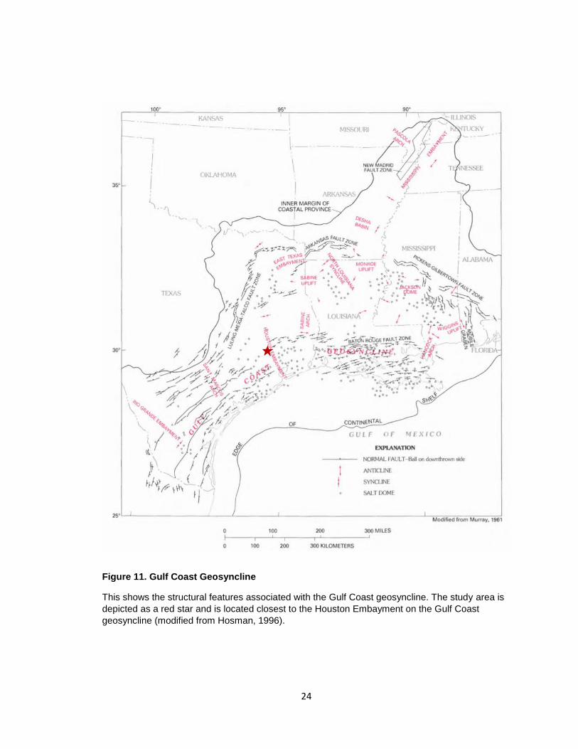
Figure 11. Gulf Coast Geosyncline
This shows the structural features associated with the Gulf Coast geosyncline. The study area is
depicted as a red star and is located closest to the Houston Embayment on the Gulf Coast
geosyncline (modified from Hosman, 1996).
25
2.2.4 THE SABINE UPLIFT
The Sabine uplift formed just northward of the Gulf Coast geosyncline
and represents a structural high that formed during the Jurassic (Figure 12). The
uplift was submerged during the Tertiary due to the deposition marine clay in the
Midway group associated with a shallow marine environment. The Wilcox group
forms the surface and has remained a structural high since the Tertiary (Lea,
McFarland and Waters, 1955). There are also many structural elements
superimposed upon the uplift, but they are not significant regionally.

26
Figure 12. Regional Structures in the Texas Gulf Coast
This figure shows the primary regional structures within the Gulf Coast, including salt domes and
nearby uplifts. The red star represents the approximate location of the study area (Modified from
Lea, McFarland and Waters, 1955).
One of the major regional structures along the Texas Gulf Coast are
normal faults. There are three major fault systems located near the study area
and they are the Luling-Mexia-Talco fault zone, Balcones fault zone and the Mt.
Enterprise fault zone (Figure 13).

27
Figure 13. Major Regional Fault Zones
The Luling-Mexia-Talco fault zone, Balcones fault zone and Mt. Enterprise fault zone are shown
with dark black lines that mark the northern extent of the Gulf of Mexico. These fault zones are
located in central Texas near Austin and San Antonia and extend westward to Del Rio, northward
to Dallas and east into Louisiana. The study area is represented by a red star (Modified from
Ferrill and Morris, 2008).
Mt. Enterprise
Fault Zone

28
2.2.5 LULING-MEXIA-TALCO FAULT ZONE
An important fault zone in the area is the Luling-Mexia-Talco fault zone
which extends northeastward across southern and southeastern Texas (Hosman,
1996). In northeastern Texas the trend of the zone turns eastward. The major
faulting episodes occurred during the Early Cretaceous and Miocene (Woodruff
Jr., 1980). These faults are associated with the Gulf Coast geosyncline. The
zone is a system of en-echelon grabens several miles across and normal faults
(Hosman, 1996). The normal faults in the system mark the boundary between the
Edwards plateau uplands and the Gulf Coast plains (Woodruff Jr., 1980). Strike-
oriented growth faulting also occurs in zones of varying extent throughout the
Gulf Coastal Plain. All are associated with subsidence of the Gulf Coast
geosyncline, and at least some are still active. A few faults, mostly in the
southeastern part of the Gulf Coastal Plain, are at approximate right angles to the
general strike of the growth-fault system (Hosman, 1996). The reasons for the
origin and orientation of these faults are not known but could be caused by salt
movement because they mark the updip limit of the Louann salt (Hosman, 1996;
Figure 14).

29
Figure 14. Cross Section of Mexia-Talco Graben
This figure shows the Mexia-Talco graben which is also the updip limit of the Louann Salt. The
graben system was facilitated by the southward extension caused by salt gliding (Wood and
Giles, 1982).
30
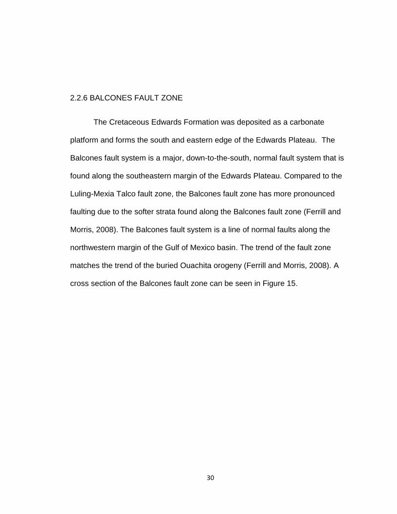
2.2.6 BALCONES FAULT ZONE
The Cretaceous Edwards Formation was deposited as a carbonate
platform and forms the south and eastern edge of the Edwards Plateau. The
Balcones fault system is a major, down-to-the-south, normal fault system that is
found along the southeastern margin of the Edwards Plateau. Compared to the
Luling-Mexia Talco fault zone, the Balcones fault zone has more pronounced
faulting due to the softer strata found along the Balcones fault zone (Ferrill and
Morris, 2008). The Balcones fault system is a line of normal faults along the
northwestern margin of the Gulf of Mexico basin. The trend of the fault zone
matches the trend of the buried Ouachita orogeny (Ferrill and Morris, 2008). A
cross section of the Balcones fault zone can be seen in Figure 15.

31
Figure 15. Cross Section of Balcones Fault Zone
This figure shows a cross section of normal faults within the Balcones Fault Zone. These faults
offset the Trinity Group, Edwards Group along with the Upper confining unit. Groundwater flow
patterns and aquifers are also shown (Modified from Barker and Ardis, 1996).
NW SE
32
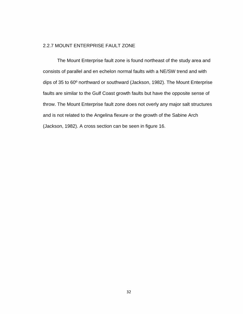
2.2.7 MOUNT ENTERPRISE FAULT ZONE
The Mount Enterprise fault zone is found northeast of the study area and
consists of parallel and en echelon normal faults with a NE/SW trend and with
dips of 35 to 60º northward or southward (Jackson, 1982). The Mount Enterprise
faults are similar to the Gulf Coast growth faults but have the opposite sense of
throw. The Mount Enterprise fault zone does not overly any major salt structures
and is not related to the Angelina flexure or the growth of the Sabine Arch
(Jackson, 1982). A cross section can be seen in figure 16.

33
Figure 16. Cross Section of the Mount Enterprise Fault Zone
This figure shows the Mount Enterprise Fault Zone which is an east-west oriented graben that runs through southern Rusk County. There is a greater thickness of the Louann Salt in the southern portion of the graben which could have been caused by upwelling of salt by sediment load (Wood and Giles, 1982).
2.2.8 EAST TEXAS EMBAYMENT
The East Texas embayment and the North Louisiana syncline form a
single major geosyncline that arcs around the northern half of the Sabine uplift
(Figure 11). The initial deformation that produced this large regional depression
was likely associated with the Ouachita orogeny. The Gulf Coast Geosyncline

34
has not received sedimentation since the withdrawal of the sea in the Tertiary
(Hosman, 1996).
2.2.9 RIO GRANDE EMBAYMENT
The Rio Grande embayment in southern Texas is a more pronounced
depression than the Houston embayment and these two embayments are
separated by the San Marcos arch (Figure 11 and 12). The axis of the Rio
Grande embayment trends east-southeast, whereas the axis of the San Marcos
arch strikes more southeast. During the late Mesozoic uplift the Rio Grande
embayment became a primary source of syntectonic sedimentation (Oldani,
1986). Tectonic sediment also accumulated in the embayment in the Oligocene
when basin and range deformation was occurring (Oldani, 1986).
2.2.10 SALT DOMES
Salt domes are common in the Gulf Coastal Plain. Hosman says that the
largest concentration of domes extends along the coast from the southeastern
corner of Texas to the southeastern tip of Louisiana (Hosman, 1996). The salt
domes formed from the Louann Salt and its age is estimated to range from

35
Triassic to Late Jurassic. Salt accumulation occurred in East Texas and incipient
Gulf of Mexico basins from Triassic to the Middle Jurassic time (Garrison, 1973).
Garrison postulated that the thick accumulations of salt led to a tectonically
unstable area where there is a high degree of mobility. The plastic flow of bedded
salt into pillows or similar structures began in the Late Jurassic and Early
Cretaceous time in response to density differences between the salt and the
accumulating overburden (Hosman, 1996). The pillows of salt moved upward in
the form of diapirs, domes or ridges and gained and gave continuing relief from
growing pressure of the overburden. Salt domes then grew
penecontemporaneously with surrounding sedimentation. The domes grew and
moved in a series of pulses of isostatic adjustments as changing equilibriums
were met (Hosman, 1996). The underlying salt flowed toward the top of the dome
and this process is known as the rim-syncline effect (Hosman, 1996). Faulting
then formed adjacent to the dome (Figure 17). A cap rock overlies the salt domes
and can show impurities in the salt that remained after salt dissolution by
groundwater (Hosman, 1996).

36
Figure 17. Faulting Around Salt Domes
This model shows the relationship between faulting and rising salt domes. This model is an
analog for the faults found around salt domes in north Harris County, not far from the study area
(Engelkemeir et al., 2010).

37
2.3 STRATIGRAPHY
The stratigraphy of the eastern Gulf Coastal Plain of Texas is very similar
to the stratigraphy in other parts of the Gulf of Mexico. The following figure shows
the stratigraphy of the Gulf of Mexico through the Cenozoic (Figure 18).
Figure 18. Stratigraphic Column of the Texas Gulf Coast
This figure shows the Stratigraphic Column of the Gulf Coast of Texas. The surficial lithologic
units can be seen outlined in red. The main units in the study area are the Lissie Formation and
the Willis Formation (Baker, 1994).

38
A stratigraphic atlas of the surface geology in the study area can be seen
in Figure 19 below. The two primary units in the study area are the Lissie Sand
and the Willis Clay.
Figure 19. Stratigraphic Atlas of the Texas Gulf Coast
This shows surficial geology of Texas along with the outline of the Gulf Coast. The red star shows where the study area is located. Modified from USGS.
Qal
Qal
Qd
Qbs
Ql Qwc
Pg
Mf
Mo
Mc

39
The study area specifically involves the eastern Gulf Coast Plain in
Montgomery, Texas. The oldest sediments were deposited in the Paleozoic and
include the Ouachita facies, but have been deeply buried. The youngest
sediments were deposited in the Quaternary and include alluvium. Drilling
downward, a well in this area would penetrate over 100 different stratigraphic
units from the Mesozoic and Cenozoic eras (Baker, 1994). Baker postulated that
these deposits are estimated to be 50,000-60,000 feet thick near the coastline
and are disrupted by fault systems.
2.3.1 PRE-JURASSIC
Any knowledge of pre-Jurassic geology in the Gulf Coastal Plain is very
limited, especially in the southern part of the area where the extreme depths of
these strata place them beyond the interest of petroleum exploration drillers and
often beyond the reach of their equipment. Paleozoic and Mesozoic rocks
underlie Cenozoic coastal deposits at the surface (Waters, McFarland and Lea,
1955). No rocks from the Triassic have been found in the Texas Gulf Coastal
plains, northern Mexico or Louisiana, but it is possible that they may be
underneath the younger strata.
40
2.3.2 JURASSIC
Jurassic deposits underlie the inner margin of the Texas Coastal Plain but
are not exposed. The principal rocks are sandstone, shale, limestone, dolomite,
and evaporites, which suggest deposition under varied environments (Waters,
McFarland and Lea, 1955). Gulfward tilting was nearly continuous although there
were unconformities that indicate periods of uplift and erosion. Thickening of the
marine facies suggests deepening of the East Texas basin during Late Jurassic
to Early Cretaceous time. In the basin there are more than 5,800 feet of Jurassic
sediments which pinch out before reaching the surface (Waters, McFarland and
Lea, 1955). During this time the Cotton Valley group formed and extended from
east Texas to Alabama. The Cotton Valley group consisted of sandstone, shale
and limestone and now underlies the northern coastal plain of the Gulf of Mexico
(Dyman and Condon, 2006).
2.3.3 CRETACEOUS
During the Cretaceous Period carbonates such as the Edwards Group,
Glen Rose Formation, Georgetown Formation, Del Rio Formation, Buda
Limestone, Eagle Ford Formation and the Austin Group were deposited in south-
central Texas as a part of a regionally extensive carbonate-dominated sequence
(Ferrill and Morris, 2008).

41
In the lower Cretaceous, sediments were deposited by a northwestward
transgressing sea. This resulted in the deposition of Trinity, Fredericksburg, and
Washita strata in the coastal province and further inland. The sediments reflect
varied environmental conditions, but the dominant rocks are limestones in the
upper part and clastics in the lower part (Waters, McFarland and Lea, 1955).
In the upper Cretaceous, the primary lithologies that were deposited were
sandstone, shale, marl, and chalk. These beds rest on the Washita group
throughout most of the Texas Coastal Plain and in the northeast, they are on
older Comanche strata (Waters, McFarland and Lea, 1955). The Woodbine
Group, described as having alternating layers of sandstone and shale is the
oldest of the Upper Cretaceous groups in the Gulf of Mexico. The Woodbine has
been traced in the subsurface as far south as Brazos and Grimes counties. The
overlying unit is the Eagle Ford, which is absent on the Sabine uplift and is
thickest in the East Texas basin. The Eagle Ford thins over the San Marcos arch
and thickens southwestward to the Mexican border. The Austin group consists of
chalk and marl over most of Texas, but in the northeastern part the dominant
lithologic types are chalk, clay, and sand (Waters, McFarland and Lea, 1955).
The thickness of the Austin group varies from 1,400 feet on the western flank of
the Sabine uplift to more than 3,600 feet in the East Texas basin. Southwestward
it varies in thickness from 1,900 feet on the San Marcos arch to more than 4,300
feet in the Rio Grande embayment (Waters, McFarland and Lea, 1955). The

42
distribution of the clastic Woodbine suggests deposition in a shallow basin with
the maximum percentage of sandstone occurring on the west flank of the Sabine
uplift. Volcanic activity outside Texas supplied large amounts of ash in northeast
Texas during this time (Leah, McFarland and Waters, 1955).
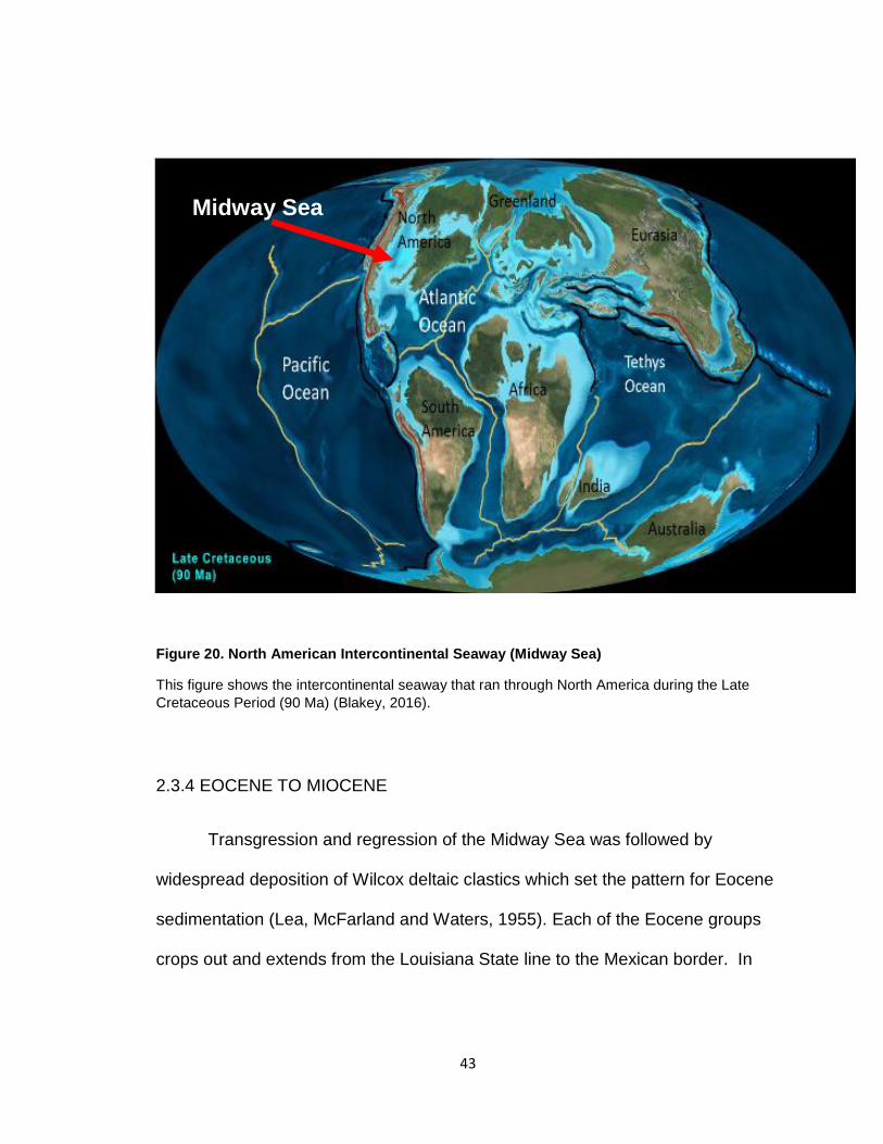
The encroachment of the Midway Sea at the close of the Cretaceous
Period began a succession of alternating marine and non-marine depositional
cycles that lasted throughout the Paleocene and Eocene Epochs (Hosman,
1996) (Figure 20). This can also be seen through the varying lithologies present
in the area. The marine interval during which sediments of the Midway Group
were deposited lasted the entire Paleocene Epoch. This was the longest and
most expansive of the Cenozoic depositional cycles (Hosman, 1995). The
maximum point of withdrawal was the Gulf Coast geosyncline, and marine
deposition there was continuous. Thus, a marine facies equivalent exists for the
entire continental sequence (Hosman, 1996).
43
Figure 20. North American Intercontinental Seaway (Midway Sea)
This figure shows the intercontinental seaway that ran through North America during the Late
Cretaceous Period (90 Ma) (Blakey, 2016).
2.3.4 EOCENE TO MIOCENE
Transgression and regression of the Midway Sea was followed by
widespread deposition of Wilcox deltaic clastics which set the pattern for Eocene
sedimentation (Lea, McFarland and Waters, 1955). Each of the Eocene groups
crops out and extends from the Louisiana State line to the Mexican border. In
Midway Sea

44
the subsurface of the Texas Coastal Plain, the Wilcox increases from 767 feet
updip in Zavala County to nearly 7,000 feet downdip in Harris County (Lea,
McFarland and Waters, 1955). Unconformably above the Wilcox is the Mount
Selman Formation, which is divided into three members (Figure 18). The oldest
is the marine Reklaw that thickens abruptly downdip across a zone of strike
parallel normal faults in the San Marcos arch area, indicating a Wilcox flexure
(Stoneham, 1953). The Queen City deltaic sand thickens from Polk County
southwestward to more than 3,400 feet in McMullen County. This suggests that
the source of Gulf Coastal Plain sediments has shifted from northeastward to
northwestward. The fossiliferous Weches is the top member of the Mount
Selman. The Sparta Formation thickens from the southwest toward the east into
South Louisiana where it is an important oil-producing formation. It is overlain by
the glauconitic fossiliferous brown shales of the Cook Mountain which in turn is
overlain by the marine sands and shales of the Yegua. The Jackson marly shales
and marine sandstone layers are the youngest Eocene group (Figure 18).
Eocene sediments thicken gulfward and the predominant down dip lithology is
shale. One well in Goliad County penetrated 10,000 feet of Eocene section
without reaching the Midway, and other areas may be underlain by greater
thicknesses (Stoneham, 1953).

45
The only strata of Oligocene age in the Texas Coastal Plain are beds
forming a marine wedge overlying the Jackson and underlying the lower
Catahoula-Frio sandstone (Figure 18).
The Miocene sediments of Texas primarily consist of ashy clay, shale, and
sand. Miocene aged strata are the most productive units in the Gulf of Mexico
(Hentz and Zeng, 2003). Southward-flowing streams transported heavy loads of
sediments and volcanic material and the ultimate deposition took place in
marshes, lagoons, and along beaches forming barrier islands and deltas, which
approached or were on the continental shelf (Berryhill et. al, 1987). In ascending
order, the Miocene units are: lower Catahoula-Frio, marine Catahoula, upper
Catahoula, Oakville, and Lagarto (Berryhill et. al, 1987; Figure 18). Miocene
sediments thicken greatly gulfward and in the subsurface it is difficult to establish
the upper and lower boundaries of the Oakville and Lagarto Formations. The
Catahoula group is 3,600 feet thick in Jackson County and 5,300 feet in Refugio
County (Berryhill et. al, 1987). Many of the major down-to-the-coast faults show a
greater thickness of Miocene on the downthrown side. This thickening indicates
movement contemporaneous with deposition. In the Gulf Coast salt-dome area
these fault zones are less prominent and local structural features are more
generally related to salt movement (Berryhill et. al, 1987).

46
2.3.5 PLEISTOCENE AND HOLOCENE
On the surface, the primary formations found in the study area were the
Pleistocene aged Lissie Sand Formation and Willis Clay Formation (Figure 18).
The Pleistocene gravels were also found in the study area and are associated
with the stream channels of the Coastal Plain. Recent sediments have been
deposited along the coast as sand dunes, beach sands, terrace material and
alluvium. In part, these units extend out under the Gulf of Mexico. The continental
shelf narrows from 13 miles at the Louisiana-Texas line to 50 miles at the
Mexican border (Lea, McFarland and Waters, 1955).
2.3.5.1 LISSIE FORMATION
Pleistocene deposits units constituted the last major depositional episodes
in the northwestern Gulf Coast Basin. The Pleistocene highstand fluviodeltaic
progradation deposited the Lissie Sand and terminated during pre-Holocene
sedimentation. The early phase of the Lissie deposition was initiated by a sudden
flexing of the coastal area which produced an even sheet of gravel, sand, sandy
clay, and much ferruginous material in the form of concretionary nodules and
cementing material (Metcalf, 1940). The second phase of the cycle began when
the streams started to in-trench into this plain, and to erode and transport the
interior portions of the Lissie toward the coast. This process gradually developed

47
channels which cut deeper into the up-dip phases of the Lissie and into older
formations (Metcalf, 1940). The type locality is at the town of Lissie, in Wharton
County, Texas. The Lissie Formation (Pleistocene) consists of thick beds of
sands with lens-shaped bodies of gravel, interspersed with clay beds (Doering,
1935). The maximum outcrop thickness for the Lissie Formation is estimated to
be about 600ft. Lissie sediments consist of reddish, orange and gray, fine-to
coarse-grained and cross-bedded sands, and include abraded fossils and lentils
of gravel of varied composition. In the subsurface, Lissie floodbasin sediments
are bluish and greenish gray (Solis, 1981). Doering also says that the slope of
the top surface of the Lissie is about 5 feet per mile, while that of its base, which
is the top of the Willis, averages about 20 feet per mile. This discordance in rate
of dip gives the Lissie a coastward thickening of about 15 feet per mile (Doering,
1935). At the surface, the Lissie Sand was found to cover 30% of Montgomery
County (USGS, 2018).

48
2.3.5.2 WILLIS FORMATION
The Willis Formation is primarily composed of clay and secondarily
composed of silt. The major lithologic constituents are coarse-to-fine grained
detrital sediments with some gravels intermixed. The gravels formed from
channel facies and the formation itself was orange-brown colored, gravelly,
coarse-to-fine sand with lenses of red, sandy silt and gray clay that is
approximately 30-200 feet thick (Moore and Wermund, 1993). The type locality
for the Willis Clay is Willis, Texas which is approximately 10 miles north of the
study area. At the surface, the Willis Clay covers 50% of Montgomery County
(USGS, 2018). Stratigraphic studies of the Willis Formation have been very
limited and future work could be done to expand upon the stratigraphy of the
formation and its depositional history.

49
CHAPTER 3
3.1 GRAVITY THEORY
Gravity surveys are conducted to determine variations in the gravitational
field of the Earth. Isaac Newton first theorized about gravity in 1687 and
formulated Newton’s Law of Universal Gravitation shortly after (Lowrie, 2007).
Newton’s Law of Universal Gravitation states that the force of attraction between
two masses (m1 and m2) is directly proportional to the product of their masses
and is inversely proportional to the square of the distances between the two
masses (Telford, et. al., 1990; Okocha, 2016). This can be defined by the
following equation:
Equation 1 𝑭 =𝑮𝒎𝟏𝒎𝟐
𝒓𝟐
G is defined as the universal gravitational constant 6.673 X 10⁻¹¹m3kg-1s-2, m1
and m2 are two masses in kilograms and r is the distance between the centers of
the masses.
Gravity is not constant throughout the Earth because the Earth is not a
perfect sphere and is not made of a homogenous material. The main factors that
influence gravity measurements are: elevation, latitude, topography, tidal

50
influence and density variations in the surface of the Earth (Telford, et. al., 1990;
Okocha, 2016).
Gravity measurements are typically measured in two ways: absolute and
relative gravity measurements. Absolute gravity measurements determine the
absolute gravity at any place while relative gravity measurements consist of
measuring the change in gravity from one place to another (Lowrie, 2007).
Absolute measurements of gravity are classically conducted with a
pendulum. Gravitational acceleration can be determined by measuring the time
of an oscillating pendulum (Telford, et. al., 1990; Okocha, 2016). More modern
methods of determining gravitation acceleration are based on observations of
free falling objects. The absolute value of gravity can be determined by fitting a
quadratic to the position of the object versus time (Lowrie, 2007). Modern
equipment uses a Michelson interferometer to accurately measure the change of
position of a free-falling object. A simplistic model of the modern free-fall method
can be seen in Figure 21. Absolute gravity methods are usually not practical for
field surveys because the absolute gravity measurements need to be conducted
over a smaller area than relative gravity measurements.

51
Figure 21. Modern Free-Fall Method for Determining Absolute Gravity
Absolute measurements of gravity can be conducted using the free-fall method. A laser beam is split along two paths to form a Michelson interferometer. The horizontal path is a fixed length while the vertical path is reflected off a corner cube retroreflector. The corner cube retroreflector is released at a known time and falls freely in an evacuated chamber to reduce air resistance. The detector determines the position of the corner cube retroreflector and the time it takes to fall (Lowrie, 2007).
The second method of measuring gravity is through relative gravity
measurements. A gravimeter is typically used in these surveys and is described
as a very sensitive balance (Lowrie, 2007). The most basic gravimeter is called a
stable type gravimeter and is comprised of a mass “m” that is suspended from a
spring with a length “so”. The force of gravity weighing down on the spring
52
causes the spring to stretch to a new length “s”. The change of length in the
spring is proportional to the restoring force of the spring and the value of gravity.
The elastic constant of the spring “k” must also be known and is usually provided
by the manufacturer of the gravimeter (Lowrie, 2007; Equation 2). This can be
defined by the following equation:
Equation 2 F = mg = -k(s-so)
Where the force of gravity in a gravimeter is defined by the elastic constant of a spring multiplied by the change in length of the spring (Lowrie, 2007).
Modern gravimeters have replaced the basic stable type gravimeter with
more sensitive types that have an additional force that acts in the same direction
as gravity and opposes the restoring force of the spring. This causes an unstable
equilibrium and is realized in the design of the spring. If the length “so” can be
made as small as possible, then the restoring force will be proportional to the
physical length of the spring instead of its extension (Lowrie, 2007). The
LaCoste-Romberg gravimeter first introduced the zero-length spring and is still
used in most modern gravimeters (Lowrie, 2007). An example of a modern
gravimeters that utilize the zero-length spring is the CG-5 Scintrex Autograv.
At any given time, a gravimeter can only measure absolute gravity or the
change in gravitational variation, because it is not possible to measure both at
the same time. Absolute and relative gravity instruments can only measure the

53
maximum of the total gravitational fields, which is the vertical component
(Telford, et. al., 1990; Okocha, 2016).
3.1.1 APPLIED GRAVITY CORRECTIONS
Gravity surveys measure the gravitational field in the Earth and are a
passive method for geophysical investigation. Passive geophysical techniques do
not input any kind of energy into the ground; instead these techniques measure
physical properties naturally occurring in the subsurface. Since the Earth is an
oblate spheroid instead of a perfect sphere there are variations in gravitational
acceleration that differ from one location to another. Gravity corrections remove
unwanted components of gravity readings that are collected in the field. Various
gravity corrections are applied to the raw gravity dataset and are discussed
further below.
3.1.2 DRIFT CORRECTION
Drift corrections account for changes caused by the instrument itself. If a
gravimeter is placed at a stationary point and readings are taken over a period of
time the gravity readings will not be consistent. The CG-5 Autograv used in this
study automatically corrects for tide and drift on measured gravity readings. Tide
corrections account for changes in gravity due to the movement of the sun and

54
the moon. Tidal corrections are also dependent on time (Telford, et. al., 1990;
Okocha, 2016).
The CG-5 Autograv gravimeter is equipped with a senor made of non-
magnetic fused quartz that is not affected by the magnetic field of variation of
less than ten times the Earth’s magnetic field ±0.5mT (Scintrex, 2012; Okocha,
2016). The quartz elastic system is a stable operating environment that allows for
long term drift of the senor to be predicted accurately and the software applies
the drift corrections to be less than 0.02 mGal per day. It is recommended that a
12-24 hour instrument drift calibration be carried out on the instrument prior to
doing any field surveying.
3.1.3 ELEVATION CORRECTION
Elevation corrections are needed to correct for topographic effects
resulting from the difference in elevation between the base station and the field
stations. Typically, there are three types of elevation corrections applied during
gravity corrections: Free-air, Bouguer and terrain corrections.
(a) Free-air correction: This corrects for variations in elevation from one
field station to another. Newton’s Law of Universal Gravitation (Equation 1)
shows that gravity decreases with the square of the distance. This means that
gravity readings will change when the gravimeter is raised or lowered; because
55
of this, the gravity data must be reduced to a datum in order to compare gravity
readings taken at various elevations within the study area. When the elevation
increases, the observed gravity readings are decreased by a vertical gradient of
0.3086 mGal/m (Telford, et. al., 1990; Okocha, 2016). The Free-air correction is
added to the observed gravity data if the field station is above the datum and is
subtracted if the observed gravity data is below the datum. The datum used in
this study was the elevation of the base station because it had a lower elevation
than all of the field stations in the study area. Since all elevation values were
above the datum, they were added to the measured gravity readings. All
elevation values for this study were extracted from LiDAR. Free-air corrections
(mGal) were calculated using the following equation:
Equation 3 Free-air correction (FAC) = 0.3086 h
Where h is defined as the elevation in meters (Telford et. al., 1990, Okocha, 2016).
(b) Bouguer correction (BC): Another type of elevation correction applied
to the observed gravity data was the Bouguer correction. The Bouguer correction
removed the effect of rock density between the measured gravity point and the
reference datum. The mass effect, or density of the rock causes measured
gravity to be greater at higher elevations than at lower elevation. Pierre Bouguer
first applied this type of correction to his work by using an assumed horizontal

56
slab with an average density of rock that was added to his observed gravity
measurements (Telford, et. al., 1990; Okocha, 2016). The equation for the
Bouguer correction is shown below:
Equation 4 Bouguer correction (BC)S = 0.4193ph
Where “p” is the average density of the surrounding Bouguer slab and “h” is the elevation in meters. An average rock density value of 2.65g/m3 was assigned to the Bouguer slab based on the geologic composition (sand and silt) of the study area (Telford et. al., 1990, Okocha, 2016).
(c) Terrain correction: The terrain correction accounts for the effect
of topography by considering the irregularities in terrain from one location to
another. Topographic highs that are located above the elevation of the gravity
base station exert an upward force on the gravimeter, which decreases the
gravitational acceleration. Valleys and topographic lows that are below the
gravity base station fails to apply a downward force on the gravimeter (Telford,
et. al., 1990; Okocha, 2016). Without terrain corrections, readings taken on top of
a mountain would have much higher gravity readings than those taken in a valley
because there is a vast difference in the amount of material beneath the
gravimeter between both locations. Topographic highs and lows effect gravity
readings, so terrains corrections must be made to account for these variations.
Since the study area was in the Gulf Coastal Plain the topography is
characterized by flat-low lying topography, so terrain corrections were not

57
necessary for this study. Gravity corrections for each survey site can be seen in
Appendix A.2.
3.2 ELECTRICAL RESISTIVITY THEORY
Electrical resistivity can be defined as “the electrical resistance per unit
length of a unit cross-sectional area of material” (Bates and Jackson, 1984).
Electrical resistivity is measured in ohm-m (Cardimona, 2002). Ohm’s law
describes the relationship between resistance, the change in surficial voltage and
the current transmitted into the subsurface by electrodes.
The relationship is shown in the equation:
Equation 5 𝑹 =∆𝑽
𝑰
(𝑅) is the resistance value, (∆𝑉) is the change in voltage at the surface and (𝐼) is the current (Ball et. al., 2004).
Direct electrical current is propagated in rocks and minerals by electrolytic
means and electronic conduction occurs where free electrons are available
(Rucker, et. al., 2010). Electrical resistivity methodology injects an electrical
current (I) into the Earth through one pair of electrodes (transmitting dipole) and

58
measures the resulting voltage potential (V) across another pair of electrodes
(receiving dipole) (Rucker, et. al., 2010). Resistance can be defined as the
amount of current flowing through a material and can vary depending on
materials and dimensions. For example, a copper wire would have less
resistance than a lead wire of the same dimensions and a short thick wire would
have less resistance than a long thin wire (Mussett and Khan, 2000; Majzoub,
2016) (Equation 2 and 3). These equations are shown below:
Equation 6 𝐫𝐞𝐬𝐢𝐬𝐭𝐚𝐧𝐜𝐞, 𝐑 = 𝐫𝐞𝐬𝐢𝐬𝐭𝐢𝐯𝐢𝐭𝐲 () × 𝐥𝐞𝐧𝐠𝐭𝐡
𝐚𝐫𝐞𝐚 𝐨𝐟 𝐜𝐫𝐨𝐬𝐬−𝐬𝐞𝐜𝐭𝐢𝐨𝐧
Equation 7 resistivity, = resistance (×) × 𝐚𝐫𝐞𝐚 𝐨𝐟 𝐜𝐫𝐨𝐬𝐬−𝐬𝐞𝐜𝐭𝐢𝐨𝐧
𝐥𝐞𝐧𝐠𝐭𝐡
The purpose of electrical resistivity surveying is to measure the distribution
of resistivity in the subsurface. Certain geologic parameters such as lithology, soil
content, water saturation and porosity influence the resistivity measurements
(Loke, 1999; Majzoub, 2016). Electrical resistivity can be measured through
multi-electrode resistivity techniques or through capacitively coupled resistivity
techniques. The OhmMapper was used in this study to image the shallow
subsurface structures and to delineate the surficial lithologic unit. The
OhmMapper computer console was worn by the operator and the dipole cables

59
were towed behind the operator. The main operating principal of the OhmMapper
is constant-current that is capacitively-coupled. Capacitively coupled resistivity
(CCR) is a method that uses a set of cables or capacitive plates instead of metal
stakes in the ground (Figure 22). When CCR is used, a voltage is applied to the
conductor inside the CCR transmitter and an electric charge forms between the
conductor and the ground (Yamashita, et. al., 2004). Insulation separates the
ground and conductor. In a CCR system, two cables are used for the transmitter
dipole and two cables are used for the receiver dipole. The Earth acts as half of a
capacitor while the cable acts as the other half of the capacitor. The insulating
jacket around the cable acts as the dielectric that separates the two halves of the
cable-earth capacitor. An AC current passes through a capacitor and a DC
current is blocked. In a CCR resistivity meter an AC current is applied to the
cable, which then passes through the earth-cable capacitor into the ground. At
the receiver side, the AC voltage is measured on the receiver cables
(Geometrics, Capacitively Coupled Resistivity).
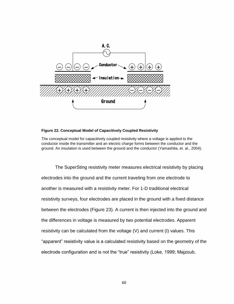
60
Figure 22. Conceptual Model of Capacitively Coupled Resistivity
The conceptual model for capacitively coupled resistivity where a voltage is applied to the
conductor inside the transmitter and an electric charge forms between the conductor and the
ground. An insulation is used between the ground and the conductor (Yamashita, et. al., 2004).
The SuperSting resistivity meter measures electrical resistivity by placing
electrodes into the ground and the current traveling from one electrode to
another is measured with a resistivity meter. For 1-D traditional electrical
resistivity surveys, four electrodes are placed in the ground with a fixed distance
between the electrodes (Figure 23). A current is then injected into the ground and
the differences in voltage is measured by two potential electrodes. Apparent
resistivity can be calculated from the voltage (V) and current (I) values. This
“apparent” resistivity value is a calculated resistivity based on the geometry of the
electrode configuration and is not the “true” resistivity (Loke, 1999; Majzoub,
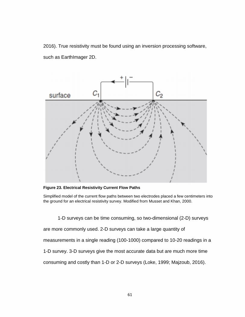
61
2016). True resistivity must be found using an inversion processing software,
such as EarthImager 2D.
Figure 23. Electrical Resistivity Current Flow Paths
Simplified model of the current flow paths between two electrodes placed a few centimeters into
the ground for an electrical resistivity survey. Modified from Musset and Khan, 2000.
1-D surveys can be time consuming, so two-dimensional (2-D) surveys
are more commonly used. 2-D surveys can take a large quantity of
measurements in a single reading (100-1000) compared to 10-20 readings in a
1-D survey. 3-D surveys give the most accurate data but are much more time
consuming and costly than 1-D or 2-D surveys (Loke, 1999; Majzoub, 2016).
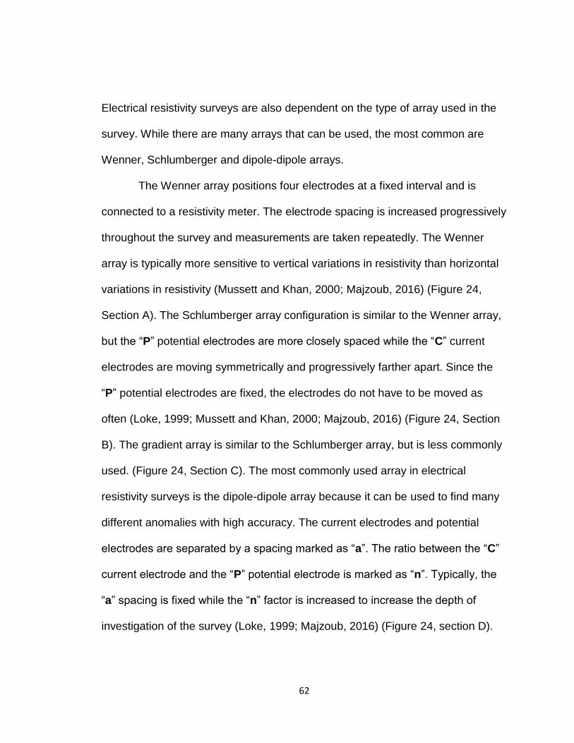
62
Electrical resistivity surveys are also dependent on the type of array used in the
survey. While there are many arrays that can be used, the most common are
Wenner, Schlumberger and dipole-dipole arrays.
The Wenner array positions four electrodes at a fixed interval and is
connected to a resistivity meter. The electrode spacing is increased progressively
throughout the survey and measurements are taken repeatedly. The Wenner
array is typically more sensitive to vertical variations in resistivity than horizontal
variations in resistivity (Mussett and Khan, 2000; Majzoub, 2016) (Figure 24,
Section A). The Schlumberger array configuration is similar to the Wenner array,
but the “P” potential electrodes are more closely spaced while the “C” current
electrodes are moving symmetrically and progressively farther apart. Since the
“P” potential electrodes are fixed, the electrodes do not have to be moved as
often (Loke, 1999; Mussett and Khan, 2000; Majzoub, 2016) (Figure 24, Section
B). The gradient array is similar to the Schlumberger array, but is less commonly
used. (Figure 24, Section C). The most commonly used array in electrical
resistivity surveys is the dipole-dipole array because it can be used to find many
different anomalies with high accuracy. The current electrodes and potential
electrodes are separated by a spacing marked as “a”. The ratio between the “C”
current electrode and the “P” potential electrode is marked as “n”. Typically, the
“a” spacing is fixed while the “n” factor is increased to increase the depth of
investigation of the survey (Loke, 1999; Majzoub, 2016) (Figure 24, section D).

63
As the “n” factor gets larger, the resolution of the survey gets poorer. This is one
of the main disadvantages of the dipole-dipole array.
Figure 24. Common Electrical Resistivity Array Configurations
The most common electrical resistivity array configurations are Wenner, Schlumberger, gradient
and dipole-dipole arrays. C is the current electrode and P is the potential electrode. Current
travels from the C current electrode while resistivity is measured by the P electrode (from Mussett
and Khan, 2000).

64
The differences in resistivity readings on a 2D pseudosection
between the different arrays can be seen below in Figure 25.
Figure 25. Apparent Resistivity for 2D Pseudosections for Various Arrays
The apparent resistivity for a 2D pseudosection over a rectangular block differs for the Wenner,
Pole-pole and Diople-dipole array. The Wenner array does not clearly define the block and
projects the block to be wider than it is. The Pole-pole array defines the block more clearly than
the Wenner array but underestimates the size of the block. The dipole-dipole array defines the
block better than the other arrays even though it overestimates the horizontal depth of the block
(Loke, 1999).
When selecting an array configuration for an electrical resistivity survey it
is important to consider the size of the target along with the shape, depth and

65
resistivity contrast between the surrounding rocks (Mussett and Khan, 2000;
Majzoub, 2016). The dipole-dipole array was used in this survey due to its high
resolution and multi-channel capability.

66
CHAPTER 4
4.0 METHODOLOGY
Geophysical research was conducted on the Big Barn fault in Montgomery
County, Texas. A CG-5 gravity meter was used to measure gravity and an TR4
OhmMapper and an R2 SuperSting resistivity meters were used to measure
electrical resistivity. Field observations were first completed to determine areas
with visible surface deformation. Broken up roadways that occurred within the
trend of the fault and displayed a noticeable decrease/increase in elevation were
examined. A Brunton compass was used to determine the trend of fault scarps. A
Brunton compass is a clinometer that has hand level capabilities and is
commonly used to determine the trend and dip of regional geologic structures.
Gravity data was acquired using the CG-5 Autograv and was used along
various roadways that bisect the fault line. The CG-5 Autograv has a resolution of
1 microGal with a standard deviation of <5 microGals. The gravitational force
exerted on the mass inside the instrument is balanced by a spring and an
electrostatic restoring force (Scintrex, 2008). Since faults commonly juxtapose
67
rocks of different densities, gravity surveying can be a viable tool for the
identification and detection of subsurface faults (Hatherton and Hunt, 1968).
Traditional electrical resistivity with a dipole-dipole array was used for both
the capacitively coupled and multi-electrode electrical resistivity surveys. Data
was first collected from the OhmMapper with a TR4 setup. Electrical resistivity
was also collected using a Super Sting R2 resistivity meter.
4.1 GRAVIMETRY METHODOLOGY
In this study gravity data was collected along traverses that were
perpendicular to the suspected fault line. The Scintrex CG-5 Autograv gravimeter
was used in this study. The CG-5 Autograv has a sensing element that is based
on a fused quartz spring system. The spring had a spring coefficient of -130
mGal /ºK. This coefficient allowed the spring to become stronger as the
temperature increased. The spring itself was protected from ambient
temperature, so that it maintained its spring temperature constant to within 0.5
mK under normal operating conditions (Okocha, 2016; Scintrex, 2012). The
gravimeter had an electric tilt sensor built into it that automatically compensated
for errors in instrument tilt during measurements. The CG-5 Autograv applied real
time tidal corrections based on the geographic location and the time zone
entered by the operator. A seismic filter was also incorporated into the CG-5

68
Autograv which removed micro-seismic noise due to locally induced shocks
(Okocha, 2016; Scintrex, 2012).
Measurements taken from the CG-5 Autograv provided information
pertaining to the density of the rocks underneath the surface. Variations in gravity
are due to lateral changes in the density of subsurface rocks. These variations
are very small and are typically measured in milligals (mGal). The CG-5 Autograv
also had a microprocessor-based automated gravity meter >8000mGal without
reset. The reading resolution was 0.001 mGal with a standard deviation <5
(Okocha, 2016; Scintrex, 2002).

69
A Trimble NOMAD was used as a handheld computer with an integrated
GPS receiver for navigation. The unit used Marvell PXA320 XScale 806 MHz
processor and Windows Mobile 6.1 software. It was also integrated with
quadband GSM GPRS/EDGE and GPS (WAAS / SBAS) capability (Okocha,
2016; Trimble, 2011). The main feature used on the Trimble NOMAD was the
GPS. The GPS was used to determine exact coordinates of field stations
throughout the survey (Figure 26).
Figure 26. Trimble NOMAD GPS Unit
The Trimble NOMAD handheld GPS Unit was used throughout the ssurvey to accurately determine the location of every field station.

70
4.1.1 LiDAR
LiDAR (Light Detection and Ranging) was used in this survey to determine
the elevation at every field station in order to make terrain corrections. LiDAR is a
remote sensing technology that illuminates a target area with a laser and
analyzes the reflected light in order to measure vertical distances (Okocha,
2016). The LiDAR data was collected in 2008 using Merrick's ALS50 Phase 2
sensor and the survey had a 1-meter resolution. The raw data was verified in
MARS software for complete coverage of the project area. The Houston-
Galveston Area Council contracted with Merrick & Company to fly the study area,
which exceeded 3,500 square miles. The purpose of collecting the LiDAR data
was for numerous GIS applications including flood modeling and prevention
along with general educational purposes. The dataset was in an. laz file format
and it contains elevation estimated values (in meters) using LiDAR technology.
4.1.2 DATA COLLECTION AND PROCESSING
Gravity data was collected using the CG-5 Scintrex Autograv and field
surveys were conducted from May to August, 2017 (Figure 27). A local gravity
base station was established and was visited before and after every day of field
surveying. Local base station visitations were necessary to ascertain the degree
of accuracy of the automatically applied drift corrections. The gravimeter was

71
programmed to collect three gravity readings per gravity station which were
collated together. Prior to field surveying, a walk-through was done at every field
site to determine the maximum length of surveying and other survey parameters.
The gravity surveys were conducted perpendicular to the fault line in order to
show a change in gravity from one side of the fault to the other. The survey
stations at every field site started at the upthrown side of the fault and extended
past the fault to the downthrown side of the fault.
Figure 27. Gravity Field Survey Lines
This shows the 6 field locations for the gravity studies conducted in this survey. The survey lines were conducted perpendicular to the fault line and went from the upthrown to the downthrown side of the fault. Map made in Google MyMaps.

72
The survey line lengths were at various lengths due to the presence of
anthropogenic features at each field site (Table 2). Planned survey lines were
adjusted where necessary to make accommodations for busy roadways, dense
forests and other obstructing features. An example of the field setup can be seen
in Figure 28.
Table 2. Gravity Field Site Information
The following table shows the various line lengths for each of the 6 field sites examined in this
survey.
Field Site Line Length (m) Station Spacing
(m) Number of Station Readings per
Field Site
1 150 25 7
2 90 15 7
3 150 25 7
4 125 25 6
5 200 25 9
6 200 25 9

73
Figure 28. Field Setup of Gravimeter
The CG-5 Gravimeter was used in this study to complete field work. In this picture the surveyor is
leveling the gravimeter by adjusting the dials at the bottom of the stand. The right figure shows
the faceplate of the CG-5 Autograv (Scintrex, 2012).
All relative gravity readings measured for this survey were tied to a pre-
established absolute gravity base station. The absolute gravity base station was
located at latitude N 29° 44.2’ and longitude W 95° 25.1'. This absolute gravity
base station is located southwest of downtown Houston (Figure 31). The
absolute gravity information of the base station was retrieved from the
International Gravimetric Bureau website, http://bgi.omp.obs-mip.fr/data-
Gravimeter
Stand
CG-5 Autograv
Gravimeter

74
products/Gravity-Databases/Reference-Gravity-53-Stations (Figure 29). This
absolute base station is the closest one to the study area and it is an open and
easily accessible. The absolute gravity was measured in July of 1967 and was
found to be 979283.720 mGal with an estimated accuracy of ± 0.1mGal. A local
gravity base station was also established and was visited before and after every
survey to ensure accuracy of the gravimetry data.

75
Figure 29. Absolute Gravity Base Station
Information about the absolute gravity base station used in this study is shown.

76
4.2 CAPACITIVELY COUPLED RESISTIVITY METHODOLOGY
A multichannel OhmMapper was used that had one transmitter and four
receivers (TR4). The OhmMapper consists of transmitter electronics and
batteries along with two transmitting dipole cables. The transmitter was towed by
a non-conductive tow link that was connected to the receivers. The receivers
consisted of the transmitter electronics, batteries and dipole cables. The received
voltage level was converted into a digital signal by an optical wand and was
transmitted to the data logger that was carried by the operator. The data logging
console (DataMapper) was attached to the operator at the waist (Figure 30). The
dipole-dipole array was selected for this survey because the data is plotted in a
pseudosection with each measurement having apparent resistivity data plotted at
the midpoint between two poles and a depth half the distance between two poles
(AGI, 2005). The main advantage of the dipole-dipole array is its high resolution
and multi-channel capability.

77
Figure 30. Field Setup for OhmMapper
This study used the TR4 setup which had one transmitter and four receivers. The transmitter had
dipole cables on either side of it and a non-conductive tow-link cable that attached another dipole
cable to the four receivers. The last receiver was attached to a dipole cable that attached to a
weight that then attached to a fiber optic isolator cable. The fiber optic isolator cable was attached
to the DataMapper that was worn at the waist of the operator (Modified from Geometrics
Operation Manual, 2001).

78
The specifications for the OhmMapper resistivity meter include the main
operating principle, operating range, cycle rate, data storage capacity, transmitter
specifications and receiver specifications (Table 3).
Table 3. OhmMapper Specifications
Specifications for the OhmMapper include operating principle, operating range, cycle rate, data
storage, transmitter specifications and receiver specification. A TR4 setup was used in this study
which used one transmitter and four receivers.
In this study the dipole-dipole array was exclusively used to measure
electrical resistivity. Not all eight field sites were accessible with the OhmMapper
resistivity meter due to a large amount of traffic in an urban environment and
anthropogenic barriers such as buildings and houses. Three of the eight field
sites were suitable for data collection using the OhmMapper resistivity meter.

79
4.2.1 FIELD SETUP
For each of the three surveys conducted with the OhmMapper resistivity
meter a specific grid orientation had to be considered. For each field site, data
collection was initiated on the downthrown side of fault and progressed to the
upthrown side of the fault. This was done to keep consistency throughout the
surveys. The signal sample and data logging rate was set to two times per
second with an operating range of less than one Ohm Meter to greater than
100,000 Ohm Meters. The Data Mapper console was attached to the operator at
the waist and the resistivity system was towed behind the operator as the
operator walked the survey line. Once the entire traverse has been surveyed to
include at least 25 meters past the suspected fault, data collection ceased. For
the second line of data collected at each field site, the line was relocated by a
distance of 5 meters along the fault line (in the x-direction). The line was then
dragged to the downthrown side of the fault and entire line was dragged at least
25 meters past the suspected fault line (Figure 31).

80
Figure 31. Grid Orientation for OhmMapper Surveys
For every field site that used the OhmMapper, the line was pulled from the downthrown to the upthrown side of the fault and was then moved over 5 meters and surveying continued.
4.2.2 DATA PROCESSING
All data stored on the console was downloaded to a desktop computer via
PC communication cables. Individual datasets from the capacitively coupled
resistivity surveys were then uploaded to the MagMap 2000 software, which
intakes raw resistivity data and outputs representative pseudosections. Once the
data files were uploaded to Magmap2000 software, survey orientation and data
type were selected (Figure 32). All surveys were conducted in a bidirectional
orientation along the Y axis.

81
Figure 32. Grid Orientation for OhmMapper Surveys
The grid orientation was chosen for every field site once it was uploaded into the MagMap 2000
software. The first position and position spacing were set based on each field site and the
surveys were always bidirectional along the Y-axis.

82
4.2.3 PSEUDOSECTIONS
After the grid orientation was selected, the survey lines were highlighted
and pseudosections were created for each field site (Figure 33). All
pseudosections were oriented along the Y-axis, which correlated to the
orientation of the appropriate survey lines. The pseudosections were then
exported to Earth Imager 2D in the RES2DINV output and formatted to create an
inverted resistivity section, which represents the resistivity variation across each
field site. Each line of resistivity data was uploaded into the Earth Imager 2D
software and was further processed to reduce noise and error.

83
Figure 33. Capacitively Coupled Resistivity Pseudosection from Field Site 2
Raw data is shown as depth (y-axis) vs. the length of the line (x-axis). The darker blue color represented lower resistivity readings, while darker red colors represented higher resistivity readings.
The pseudosection represented a relative distribution model of the
apparent resistivity values collected during the field survey. The data had to be
inverted in order to produce a true Earth resistivity model. Uploaded data was
inverted using the smooth model inversion or Occam’s inversion that finds the
smoothest model to fit the collected data. Surface settings were used for all data
collected in the survey (Figure 34).

84
Figure 34. Initial Settings in Earth Imager 2D for OhmMapper Survey
The Smooth Model Inversion was selected as the inversion method for all data collected by the SuperSting resistivity meter. EarthImager 2D utilized this and the Surface setting was always selected as the default.

85
4.2.4 DATA MISFIT
The percentage of mismatch between data collected in the field and the
resulting inversion model was calculated by the inversion software and reported
as mismatched or the Root Mean Square (RMS). Noise data collected during the
survey could be attributed to surface background resistance or anthropogenic
features such as telephone poles, wire fences and pipelines. Noise is
automatically accounted for in the initial settings and less weight is given to it in
the inverted section. A 3% maximum repeat error was applied in the Resistivity
Inversion settings (Figure 35). While this setting helps reduce noise, it does not
completely remove it.

86
Figure 35. Resistivity Inversion Settings in Earth Imager 2D Software
The estimated noise for all surveys was set to 3% under the Resistivity Inversion settings in the
Earth Imager 2D software. All other amounts were set to the default amounts for all surveys.
Data that was poorly fitted was manually removed based on the relative
misfit observed in the data misfit histogram (Figure 36). A data misfit histogram
for each data set allows the operator to remove small amounts of noisy data to

87
lower the RMS value of the survey. The histogram is automatically generated
after every inversion was fully converged.
Figure 36. Data Misfit Histogram for Capacitively Coupled Resistivity Field Survey Site 2
A screenshot was taken of the data misfit histogram for the capacitively coupled resistivity survey
site 2. The figure shows the relative data misfit % (x-axis) versus the number of data (y-axis). In
the above example, 3 out of a total 111 noisy data points were removed.
Any misfit data was removed incrementally before running the inversion
processes again. The maximum data removed for all conductively coupled
resistivity surveys was 15%. This process was repeated until the Root Mean
Squared Error was reduced to <10%. A data misfit crossplot was examined for
every field site to see the measured vs. apparent resistivity data (Figure 37).

88
Figure 37. Crossplot of Measured vs. Predicted Apparent resistivity for Capacitively Coupled Resistivity Surveys
This shows the measured apparent resistivity (x-axis) versus the predicted apparent resistivity (y-axis) for field site 2. The green line represents the predicted apparent resistivity while the data points overlain on top of it.

89
4.3 MULTI-ELECTRODE ELECTRICAL RESISTIVITY METHODOLOGY
The electrical resistivity data was collected using a Super Sting R2 two-
channel resistivity meter produced by Advanced Geosciences, Inc. that utilized
the dipole-dipole array type with 28 electrodes at 4-meter or 6.5-meter spacing.
Resistivity data was collected at Field Sites 1, 2, 5 and 7 (Figure 38). Resistivity
data could not be collected at other sites (3, 4 and 6) because the survey cables
would have intersected busy driveways or intersections. The dipole-dipole array
was selected for this survey because the data is plotted in a pseudosection with
each measurement having apparent resistivity data plotted at the midpoint
between two poles and a depth half the distance between two poles (AGI, 2005).
The main advantage of the dipole-dipole array is its high resolution and multi-
channel capability. The Super Sting resistivity meter was powered by two twelve-
volt batteries and the surveys were conducted in Boost mode for faster surveying
time (Figure 39).
The survey length varied depending on the electrode spacing used and
were chosen based on the desired depth of investigation and the resolution
required to delineate a fault plane (Table 4). Smaller electrode spacing was not
considered because it would have given a much shallower depth of investigation
of the subsurface. All of the data were processed using EarthImager 2D software
by Advanced Geosciences, Inc.

90
Figure 38. Super Sting Field Sites
Survey sites examined with the R2 SuperSting. Field Sites 1, 2, 5 and 7 were examined in this
study. Map created in Google Maps.
Figure 39. SuperSting R2 Electrical Resistivity Meter Setup
The SuperSting R2 electrical resistivity meter is produced by Advances
Geosciences Inc. This image shows the SuperSting console, switchbox and power supply.
Electrode cables are attached to the switchbox and are not shown.

91
Table 4. SuperSting Survey Sites and Field Parameters
4.3.1 COMMAND FILES
Command files were made prior to conducting the multichannel resistivity
surveys and were created in the administrator software on the tablet associated
with the SuperSting and produced by Advanced Geosciences (Figure 40). The
R2 SuperSting unit used in the survey was Wi-Fi enabled and was synchronized
with the AGI SuperSting Manager application pre-installed on the tablet. The
application included a Command Creator option that allowed command files to be
produced. The command file for the 28-electrode dipole-dipole survey was
created in the mobile application and was downloaded to the SuperSting
resistivity meter via Wi-Fi___33. The command file contained the survey
Field Site Electrode Spacing Survey Length Array Maximum Depth of
Investigation
1 6.5 meters 176 meters Dipole-Dipole 32 meters
2 4 meters 108 meters Dipole-Dipole 26.1 meters
2 6.5 meters 176 meters Dipole-Dipole 42.5 meters
5 6.5 meters 176 meters Dipole-Dipole 24.7 meters
7 6.5 meters 176 meters Dipole-Dipole 42.5 meters
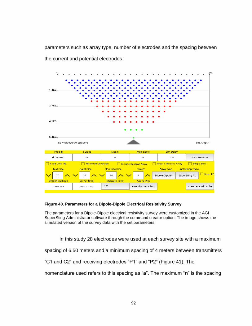
92
parameters such as array type, number of electrodes and the spacing between
the current and potential electrodes.
Figure 40. Parameters for a Dipole-Dipole Electrical Resistivity Survey
The parameters for a Dipole-Dipole electrical resistivity survey were customized in the AGI SuperSting Administrator software through the command creator option. The image shows the simulated version of the survey data with the set parameters.
In this study 28 electrodes were used at each survey site with a maximum
spacing of 6.50 meters and a minimum spacing of 4 meters between transmitters
“C1 and C2” and receiving electrodes “P1” and “P2” (Figure 41). The
nomenclature used refers to this spacing as “a”. The maximum “n” is the spacing

93
ratio between “C1 and P1” electrodes to the “C2 and C1” or “P1 and P2” dipole
separation. For this survey the “n” spacing was set to 8. For dipole-dipole arrays,
the “a” spacing is initially kept fixed and gradually increased along with the “n”
factor to allow for greater depth penetration (Loke, 1999; Majzoub, 2016). The
spacing between the dipole-dipole pairs was dependent on the electrode spacing
used in the field. The parameters set in the command file automatically dictate
the geometry of the survey (Figure 41). Since the software dictates the geometry
of the survey automatically it is not necessary to move the electrodes during the
survey.
Figure 41. Dipole-Dipole Electrode Configuration
The Dipole-Dipole array is shown as a simplified model of the electrode configuration for the
survey. “n” is the distance ratio between the dipole separation and “a” is the spacing between the
transmitting and receiving electrodes (Majzoub, 2016).

94
4.3.2 DATA ACQUISITION
Survey sites and lengths were limited by their access to long stretches of
roadways without intersecting driveways. A tape measure was used to measure
the correct spacing in between the electrodes. The surficial deformation was first
identified at each field site and then a flag was placed along the tape measure at
the predetermined interval to mark the proper electrode spacing for each survey.
Stainless steel stakes were hammered at the predetermined interval depending
on the length of the survey. The goal of each survey was to have the fault plane
as close as possible to the center of the survey line to attain maximum efficiency.
The two sets of cable were connected together and then the electrodes were
attached to the stainless-steel stakes. All data was collected using 28 electrodes
and a dipole-dipole array.
4.3.3 FIELD SETUP
For this study, two cable sections with 14 electrodes per cable and 28
electrodes total were used. Cable sections with electrodes 1-14 represented the
low-address section and 15-28 represented the high address section. The
SuperSting resistivity meter was placed at the high address for all surveys, as
per the recommendation of the manufacturer (Figure 42) (AGI, 2015). Two 12-
volt batteries were used in this survey and allowed the SuperSting to operate in

95
Boost mode, which has a range of 0-200 Watt instead of the main mode that is
powered by one 12-volt battery and has a range of 0-100 Watt (Figure 43).
Figure 42. Schematic of Field Surveying with SuperSting
The SuperSting was placed at the end of the high-address of the cable sections and was
attached to a switchbox and two 12-volt batteries that were the power supply. The switchbox was
used at the end of the survey since there were no further cables sections to attach together.
Figure 43. Field Setup of 28-Electrode SuperSting Survey
A 28-electrode survey was completed using electrode cables, a switchbox, a tablet that
connected to the SuperSting system and the power supply. The low-address electrode cables
were attached to the high-end address electrode cables which was then connected to the
switchbox. The SuperSting system was connected to a switchbox and two 12-volt batteries. The
SuperSting was Wi-Fi enabled so a tablet was used to remotely control the SuperSting and
monitor the survey.

96
For this survey, inversion settings were set to 1.2 second measurement
time with two measurement cycles at each electrode pair. The maximum error
percentage between measurements was set to 2% and injected current
maximum to 2000 Ma. A contact resistance test was performed at each field site
in order to ensure quality control of the survey. A contact resistance test is an
option when an automatic survey is selected and is a feature on the SuperSting
that allows the user to check the quality of the electrode coupling with the
ground. If the contact resistance was greater than 1500 ohms than the electrode
cable was repositioned, or the metal stake was hammered farther into the
ground. As the data was collected it was monitored on the tablet that was synced
to the SuperSting (Figure 44).
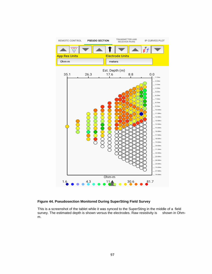
97
Figure 44. Pseudosection Monitored During SuperSting Field Survey
This is a screenshot of the tablet while it was synced to the SuperSting in the middle of a field survey. The estimated depth is shown versus the electrodes. Raw resistivity is shown in Ohm-m.
98
4.3.4 DATA PROCESSING AND PSEUDOSECTIONS
For the multi-electrode electrical resistivity surveys the electrical resistivity
data was processed using AGI’s Earth Imager 2D version 2.4.4. All data
collected from the field site was uploaded to a personal computer from the tablet
synchronized with the SuperSting resistivity meter or through a PC Com cable
produced by AGI that was attached to a Brainbox adapter for a computer. Raw
data uploaded into the Earth Imager 2D software was displayed as a
pseudosection. The pseudosection represented a relative distribution model of
the apparent resistivity values collected during the field survey. The data had to
be inverted in order to produce a true Earth resistivity model and noise was
removed incrementally before running the inversion processes again. All data
was inverted using the smooth model inversion or Occam’s inversion that finds
the smoothest model to fit the collected data. Surface settings were used for all
data collected in the survey. The maximum data removed for all multi-electrode
electrical resistivity surveys was 15%. This process was repeated until the Root
Mean Squared Error was reduced to <10%. A data misfit crossplot was examined
for every field site to see the measured vs. apparent resistivity data.
EarthImager2D was used also used for the multi-electrode resistivity data so the
software methodology is the same as what was previously mentioned in the
capacitively coupled resistivity data processing section (Figure 32-35).
99
CHAPTER 5
5.0 RESULTS
For this study three geophysical techniques were used to delineate the Big
Barn fault in Montgomery County, Texas. The first geophysical technique used
was gravity surveying and the CG-5 Autograv was used to conduct the surveys.
Gravity measurements were taken at 25m intervals six different traverses
oriented roughly perpendicular to the apparent fault line. The second geophysical
technique used in this study was a conductively coupled resistivity (CCR) survey
using the OhmMapper resistivity meter. The CCR survey was conducted at three
of the seven predetermined field sites along traverses perpendicular to the
apparent fault line. The third and final geophysical technique used was multi-
electrode electrical resistivity survey, utilizing the SuperSting R2 Wi-Fi
RES/IP/SP resistivity meter. The SuperSting resistivity meter was used at four
field sites and along traverses established in the CCR and gravity section of the
study. The location of the seven field sites are shown in figure 45.

100
Figure 45. Study Area Regional Location
The study area is shown relative to the city of the Conroe and the Woodlands, Texas. Field stations are shown with blue icons and the approximate strike of the fault line was determined to be approximately N62⁰E.
1 2 3
4 5
6 7
0.5 0 1 Mi
N
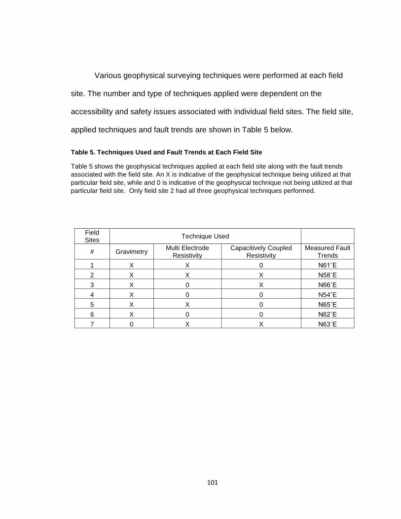
101
Various geophysical surveying techniques were performed at each field
site. The number and type of techniques applied were dependent on the
accessibility and safety issues associated with individual field sites. The field site,
applied techniques and fault trends are shown in Table 5 below.
Table 5. Techniques Used and Fault Trends at Each Field Site
Table 5 shows the geophysical techniques applied at each field site along with the fault trends
associated with the field site. An X is indicative of the geophysical technique being utilized at that
particular field site, while and 0 is indicative of the geophysical technique not being utilized at that
particular field site. Only field site 2 had all three geophysical techniques performed.
Field Sites
Technique Used
# Gravimetry Multi Electrode
Resistivity Capacitively Coupled
Resistivity Measured Fault
Trends
1 X X 0 N61˚E
2 X X X N58˚E
3 X 0 X N66˚E
4 X 0 0 N54˚E
5 X X 0 N65˚E
6 X 0 0 N62˚E
7 0 X X N63˚E
N

102
5.1 GRAVIMETRY
Gravimetry was used in this study to delineate differences in rock
densities within the study area. A previous study (Khan et. al., 2013) of the
geology of the area showed that the Lissie Sand was suspected to be on the
downthrown (southern) end of the fault line while the Willis Clay was suspected
to be on the upthrown (northern) end of the fault line. Field sites 1-6 were
examined using the CG-5 Autograv and the results of the gravity survey is shown
below for each field site (Figures 46-51).

103
Figure 46. Gravity Data from Field Site 1
(A) Study area for field site 1 along with the N 61ºE trend of the fault line measured at this field site
with a Brunton compass. This location is along Kuykendahl Road in Montgomery County, Texas. Note
that North is to the right in this image (Photo from Google Earth). (B) Plotted corrected gravity data
from field site 1. Using gravimetry, it was determined that the (southern) downthrown side of the fault
had higher gravity readings than the (northern) upthrown side of the fault. The data for this survey is
anomalous to typical gravity surveys that have higher gravity readings on the upthrown side of the
fault. This anomalous result could be due to a higher accumulation of the denser Lissie Sand on
downthrown side of the fault and the less dense Willis Clay on the upthrown side of the fault. The
Lissie Sand could also be pinching out at the fault line, leaving only the Willis Clay on the upthrown
side of the fault. Khan et. al., 2013, also had anomalous gravity data that he attributed to the density
differences between the Lissie Sand and Willis Clay near the Hockley Fault.
S N
Downthrown Upthrown
(A)
(B)

104
3726.65
3726.7
3726.75
3726.8
3726.85
3726.9
3726.95
3727
0 10 20 30 40 50 60 70 80 90 100
Co
rrec
ted
Gra
vity
(m
Gal
)
Distance (m)
Field Site 2
StationsUpthrown
Downthrown
(A) Study area for field site 2 along with the N 58ºE trend of the fault line measured at this field site
with a Brunton compass. This site was located along Cochrans Crossing Dr. in Montgomery County,
Texas (Photo from Google Maps). (B) Plotted corrected gravity data from field site 2. Using
gravimetry, it was determined that the (southern) downthrown side of the fault had higher gravity
readings than the (northern) upthrown side of the fault. The data for this survey is anomalous to
traditional gravity surveys that have higher gravity readings on the upthrown side of the fault. This
anomalous behavior could be due to a higher accumulation of the denser Lissie Sand on downthrown
side of the fault and the less dense Willis Clay on the upthrown side of the fault. Gravity readings
taken 30-40 meters along the survey line could represent the Lissie Sand interfacing with the Willis
Clay along the fault line or it may be pinching out along the fault line. Khan et. al., 2013, also had
anomalous gravity data that he attributed to the density differences between the Lissie Sand and
Willis Clay near the Hockley Fault.
Figure 47. Gravity Data from Field Site 2
N
N S
(A)
(B)

105
3697.4
3697.45
3697.5
3697.55
3697.6
3697.65
3697.7
3697.75
0 20 40 60 80 100 120 140 160
Co
rrec
ted
Gra
vity
(m
Gal
)
Distance (m)
Field Site 3
Stations
Downthrown
Upthrown
Figure 48. Gravity Data from Field Site 3
(A) Study area for field site 3 along with the N 66ºE trend of the fault line measured at this field site with a
Brunton compass. This site was located along the other side of Cochrans Crossing Dr. in Montgomery
County, Texas (Photo from Google Maps). (B) Plotted corrected gravity data from field site 3. Using
gravimetry, it was determined that the (southern) downthrown side of the fault had higher gravity readings
than the (northern) upthrown side of the fault. The data for this survey is anomalous to traditional gravity
surveys that have higher gravity readings on the upthrown side of the fault. This anomalous behavior could
be due to a higher accumulation of the denser Lissie Sand on downthrown side of the fault and the less
dense Willis Clay on the upthrown side of the fault. Khan et. al., 2013, also had anomalous gravity data that
he attributed to the density differences between the Lissie Sand and Willis Clay near the Hockley Fault.
N S (B)
(A)

106
Figure 49. Gravity Data from Field Site 4
3701.35
3701.4
3701.45
3701.5
3701.55
3701.6
0 20 40 60 80 100 120 140
Co
rrec
ted
Gra
vity
(m
Gal
)
Distance (m)
Field Site 4
Stations
Downthrown
Upthrown
(A) Study area for field site 2 along with the N 54ºE trend of the fault line measured at this field site
with a Brunton compass. This site was located at Summer Haze Circle and Green Bridge Dr. in
Montgomery County, Texas (Photo from Google Maps). (B) Plotted corrected gravity data from field
site 2. Using gravimetry, it was determined that the (southern) downthrown side of the fault had higher
gravity readings than the (northern) upthrown side of the fault. The data for this survey is anomalous
to traditional gravity surveys that have higher gravity readings on the upthrown side of the fault. This
anomalous behavior could be due to a higher accumulation of the denser Lissie Sand on downthrown
side of the fault and the less dense Willis Clay on the upthrown side of the fault. Khan et. al., 2013,
also had anomalous gravity data that he attributed to the density differences between the Lissie Sand
and Willis Clay near the Hockley Fault.
N S (B)
(A)

107
Figure 50. Gravity Data from Field Site 5
3709.35
3709.4
3709.45
3709.5
3709.55
3709.6
3709.65
0 50 100 150 200 250
Co
rrec
ted
Gra
vity
(m
Gal
)
Distance (m)
Field Site 5
Stations
Downthrown
Upthrown
(A) Study area for field site 2 along with the N 54ºE trend of the fault line measured at this field site
with a Brunton compass. This site was located along TX-242 in Montgomery County, Texas (Photo
from Google Maps). (B) Plotted corrected gravity data from field site 2. Using gravimetry, it was
determined that the (southern) downthrown side of the fault had higher gravity readings than the
(northern) upthrown side of the fault. The data for this survey is anomalous to traditional gravity
surveys that have higher gravity readings on the upthrown side of the fault. For this field site, the
variance in the gravity from the upthrown to downthrown side is minimal and could be caused by the
Lissie Sand being overlain on top of the Willis Clay throughout the field site with offset of the layers
near the vicinity of the fault. If faulting caused the layers to offset, then a slightly higher accumulation
of the Lissie Sand will be seen on the downthrown side and a higher accumulation of the Willis Clay
on the upthrown side of the fault. Khan et. al., 2013, also had anomalous gravity data that he
attributed to the density differences between the Lissie Sand and Willis Clay near the Hockley Fault.
N S (B)
(A)
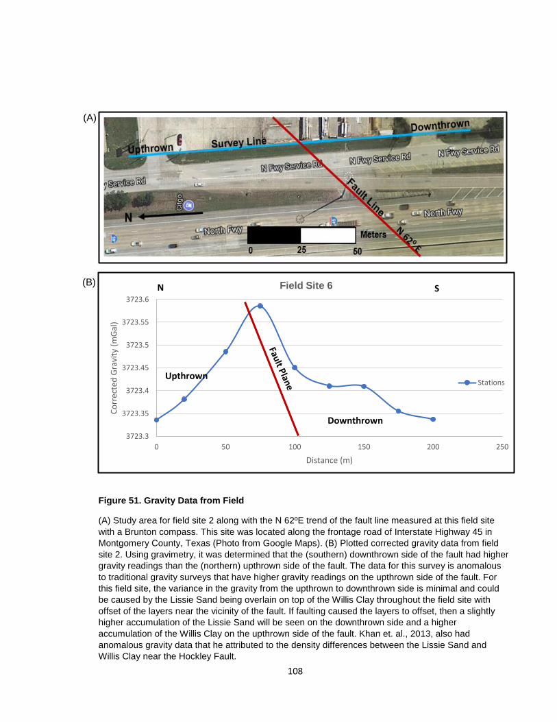
108
Figure 51. Gravity Data from Field
Electrical Resistivity Data
Ohm \
3723.3
3723.35
3723.4
3723.45
3723.5
3723.55
3723.6
0 50 100 150 200 250
Co
rrec
ted
Gra
vity
(m
Gal
)
Distance (m)
Field Site 6
Stations
N S
Downthrown
Upthrown
(A) Study area for field site 2 along with the N 62ºE trend of the fault line measured at this field site
with a Brunton compass. This site was located along the frontage road of Interstate Highway 45 in
Montgomery County, Texas (Photo from Google Maps). (B) Plotted corrected gravity data from field
site 2. Using gravimetry, it was determined that the (southern) downthrown side of the fault had higher
gravity readings than the (northern) upthrown side of the fault. The data for this survey is anomalous
to traditional gravity surveys that have higher gravity readings on the upthrown side of the fault. For
this field site, the variance in the gravity from the upthrown to downthrown side is minimal and could
be caused by the Lissie Sand being overlain on top of the Willis Clay throughout the field site with
offset of the layers near the vicinity of the fault. If faulting caused the layers to offset, then a slightly
higher accumulation of the Lissie Sand will be seen on the downthrown side and a higher
accumulation of the Willis Clay on the upthrown side of the fault. Khan et. al., 2013, also had
anomalous gravity data that he attributed to the density differences between the Lissie Sand and
Willis Clay near the Hockley Fault.
(A)
(B)

109
5.2 CAPACITIVELY COUPLED RESISTIVITY
The second geophysical technique used in this study utilized capacitively
coupled resistivity and was completed using the OhmMapper TR4 resistivity
system. The OhmMapper resistivity meter measured electrical resistivity at
shallow depths and was used to delineate the varying rock types on either side of
the fault. The downthrown side of the fault contained the Lissie Sand which
showed a higher resistivity and was shown as a warmer color (orange-red). The
upthrown side of the fault was characterized by the Willis Clay which showed a
lower resistivity and was shown as a cooler color (blue-purple). The OhmMapper
resistivity meter was used at three field sites but had multiple lines completed at
each field site. The OhmMapper resistivity meter was used at field sites 2, 3 and
7. The data collected for the OhmMapper resistivity meter is shown below for
each field site (Figures 52-54). The OhmMapper resistivity meter was not used at
field sites 1, 4, 5 & 6 due to busy roadways and driveway intersections along the
prospective survey lines.
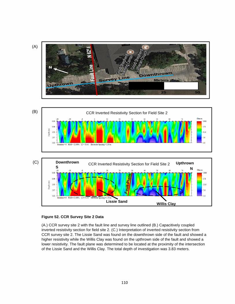
110
Figure 52. CCR Survey Site 2 Data
(A.) CCR survey site 2 with the fault line and survey line outlined (B.) Capacitively coupled
inverted resistivity section for field site 2. (C.) Interpretation of inverted resistivity section from
CCR survey site 2. The Lissie Sand was found on the downthrown side of the fault and showed a
higher resistivity while the Willis Clay was found on the upthrown side of the fault and showed a
lower resistivity. The fault plane was determined to be located at the proximity of the intersection
of the Lissie Sand and the Willis Clay. The total depth of investigation was 3.83 meters.
(A)
Upthrown
Downthrown
S
N
Lissie Sand
Willis Clay
CCR Inverted Resistivity Section for Field Site 2
CCR Inverted Resistivity Section for Field Site 2 (B)
(C)

111
Figure 53. CCR Survey Site 3 Data
(A.) CCR survey site 3 with the fault line and survey line outlined (B.) Capacitively coupled
inverted resistivity section for field site 3. (C.) Interpretation of inverted resistivity section from
CCR survey site 3. The Lissie Sand was found on the downthrown side of the fault and showed a
higher resistivity while the Willis Clay was found on the upthrown side of the fault and showed a
lower resistivity. The fault plane was determined to be at the to be located at the proximity of the
intersection of the Lissie Sand and the Willis Clay. The Lissie Sand also appears to be pinching
out above the Willis Clay on the upthrown side of the fault. The total depth of investigation was
3.83 meters.
(A)
(B)
(C)
Lissie Sand
Willis Clay
Downthrown
Upthrown
S
N
CCR Inverted Resistivity Section for Field Site 3
CCR Inverted Resistivity Section for Field Site 3

112
Figure 54. CCR Survey Site 7 Data
(A.) CCR survey site 7 with the fault line and survey line outlined (B.) inverted resistivity section
for field site 7. (C.) Interpretation of inverted resistivity section from CCR survey site 7. The
downthrown side of the fault line showed a lower resistivity while the upthrown side of the fault
showed a higher resistivity which is opposite of the trend in CCR survey site 2 and 3. This change
in lithology could be due to the nearby San Jacinto river that is located to the Northeast of the
study area. Clays from the Beaumont Formation could have accumulated on the downthrown side
of the fault. The Lissie Sand was found on the upthrown side of the survey line, but it could also
be found deeper on the downthrown side of the fault. The total depth of investigation was 3.83
meters.
(A)
(B)
(C)
CCR Inverted Resistivity Section for Field Site 7

113
5.3 MULTI-ELECTRODE RESISTIVITY
The third geophysical technique used in this study utilized multi-electrode
resistivity and was conducted using the R2 SuperSting resistivity meter. The
SuperSting resistivity meter used electrical resistivity to delineate deeper
subsurface features than the OhmMapper resistivity meter. The OhmMapper
resistivity meter had a maximum depth of four meters while the SuperSting had a
maximum depth of 32 meters. Multi-electrode resistivity was used at field sites 1,
2, 5 and 7. The data collected from the SuperSting resistivity meter at each field
location is shown below (Figures 55-59).

114
55. Multi-electrode Resistivity Survey Site 1
(A) Multi-electrode Resistivity survey site 1 with the fault line highlighted in blue red and
the survey line highlighted in blue. (B) Inverted resistivity section from survey site 1 (C)
Interpretation of the inverted resistivity section. Higher resistivity readings were shown in
red, while lower resistivity readings were shown in blue. The upper most lithologic unit in
this area was the Lissie sand and was in higher accumulation on the downthrown side of
the fault. The Willis Clay laid conformably underneath the Lissie Sand with offset in the
layers in the vicinity of the fault plane. The approximated offset of the Willis Clay was
found to be 2.8 meters. The Lissie Sand pinches out to the North on the upthrown side of
the fault. The maximum depth of the survey was 32 meters.
N
(B)
(A)
(C) Multi-electrode Inverted Resistivity Section for Field Site 1
Multi-electrode Inverted Resistivity Section for Field Site 1
S
Downthrown Upthrown
N

115
Figure 56. Multi-electrode Resistivity Survey Site 2 (4 Meter Survey)
(A) Multi-electrode resistivity survey site 2 with a NW-SE trending survey line shown in
blue and a NE striking fault trend shown in red. (B) Inverted resistivity section from field
site 2, with higher resistivity readings shown in red and lower resistivity readings shown in
blue. The electrode spacing for this survey was set to 4 meters. (C) Interpretation of
inverted resistivity section from field site 2. A normal fault was found near the center of
the survey line with the Lissie Sand being dropped down to the South. The Willis Clay
was found on the upthrown side of the fault line with an interfingering of the Lissie Sand.
The offset of the Lissie Sand at this field site was found to be 2 meters. The total depth
of this survey was 26.1 meters.
(C)
(B)
(A)
Multi-electrode Inverted Resistivity Section for Field Site 2 (4 Meter Survey)
Multi-electrode Inverted Resistivity Section for Field Site 2 (4 Meter Survey)

116
57. Multi-electrode Resistivity Survey Site 2 (6.5 Meter Survey)
(A) Multi-electrode resistivity survey site 2 with the NW-SE trending survey line outlined in
blue and the NE trending fault line outlined in red. (B) Inverted resistivity section for field
site 2 with higher resistivity readings shown in red and lower resistivity readings shown in
blue. The electrode spacing for this survey was set to 6.5 meters. (C) Interpretation of
inverted resistivity section from field site 2. A normal fault was found near the center of
the survey line with the Lissie Sand being dropped down to the South. The Willis Clay
was found on the upthrown side of the fault line with an interfingering of the Lissie Sand.
The offset of the Lissie Sand at this field site was found to be 2 meters. The total depth
of this survey was 26.1 meters.
Multi-electrode Inverted Resistivity Section for Field Site 2 (6.5 Meter Survey)
Multi-electrode Inverted Resistivity Section for Field Site 2 (6.5 Meter Survey)
(A)
(B)
(C)
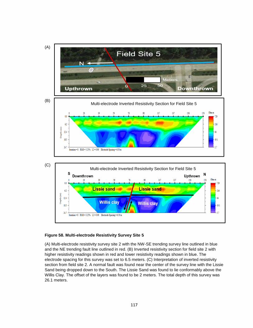
117
(A)
(B)
(C)
Figure 58. Multi-electrode Resistivity Survey Site 5
(A) Multi-electrode resistivity survey site 2 with the NW-SE trending survey line outlined in blue
and the NE trending fault line outlined in red. (B) Inverted resistivity section for field site 2 with
higher resistivity readings shown in red and lower resistivity readings shown in blue. The
electrode spacing for this survey was set to 6.5 meters. (C) Interpretation of inverted resistivity
section from field site 2. A normal fault was found near the center of the survey line with the Lissie
Sand being dropped down to the South. The Lissie Sand was found to lie conformably above the
Willis Clay. The offset of the layers was found to be 2 meters. The total depth of this survey was
26.1 meters.
Multi-electrode Inverted Resistivity Section for Field Site 5
Multi-electrode Inverted Resistivity Section for Field Site 5

118
(A)
(B)
(C)
Figure 59. Multi-electrode Resistivity Survey Site 7
(A) Multi-electrode resistivity survey site 2 with the NW-SE trending survey line outlined in
blue and the NE trending fault line outlined in red. (B) Inverted resistivity section for field
site 2 with higher resistivity readings shown in red and lower resistivity readings shown in
blue. The electrode spacing for this survey was set to 6.5 meters. (C) Interpretation of
inverted resistivity section from field site 2. A normal fault was found near the center of
the survey line with the Lissie Sand being dropped down to the South. The Lissie Sand
was found to lie conformably above the Willis Clay and the offset of the layers was found
to be 5 meters. The total depth of this survey was 42.5 meters.
Multi-electrode Inverted Resistivity Section for Field Site 7

119
CHAPTER 6
6.0 DISCUSSION
For this study gravity and electrical resistivity methods were used to
delineate the Big Barn fault in Montgomery County, Texas. After examining
existing geologic maps and through gravity and electrical resistivity techniques,
the Big Barn fault was interpreted to truncate the Lissie Sand and the Willis Clay.
Gravity data showed that the majority of the field sites (field sites 1, 2, 3, 4 and 5)
showed a higher gravity on the downthrown side of the fault than on the
upthrown side of the fault. The downthrown side of the fault was interpreted to
contain higher accumulations of the Lissie Sand. Since sandstones are generally
denser than claystones, they will naturally result in higher gravity readings.
Electrical resistivity correlated well to the gravimetry data and also showed that
the downthrown side of the fault had a higher resistivity consistent with the Lissie
Sand, while the upthrown side of the fault had a lower resistivity consistent with
the Willis Clay. The offset between the Lissie Sand and Willis Clay was found in
field sites 1, 2, 5 and 7 through multi-electrode electrical resistivity techniques.
Interpretations of the data collected at different field sites are discussed below.

120
Field Site 1
Field site 1 (Figure 60) utilized gravity and multi-electrode resistivity
techniques to delineate faulting. At this field site, the downthrown side of the fault
had higher gravity readings than the upthrown side. This contrast in gravity
readings was likely due to a higher accumulation of the denser Lissie Sand on
the downthrown side of the fault. The upthrown side of the fault had a higher
accumulation of the less dense Willis Clay. Through multi-electrode resistivity
imaging, a two-dimensional inverted resistivity section was created. The Lissie
Sand was shown as light green- red in color and represented a higher resistivity.
The Willis Clay was shown as light purple-blue in color and represented a lower
resistivity. A normal fault offset the Lissie Sand and Willis Clay by 2 meters and
the total survey depth was 32 meters.
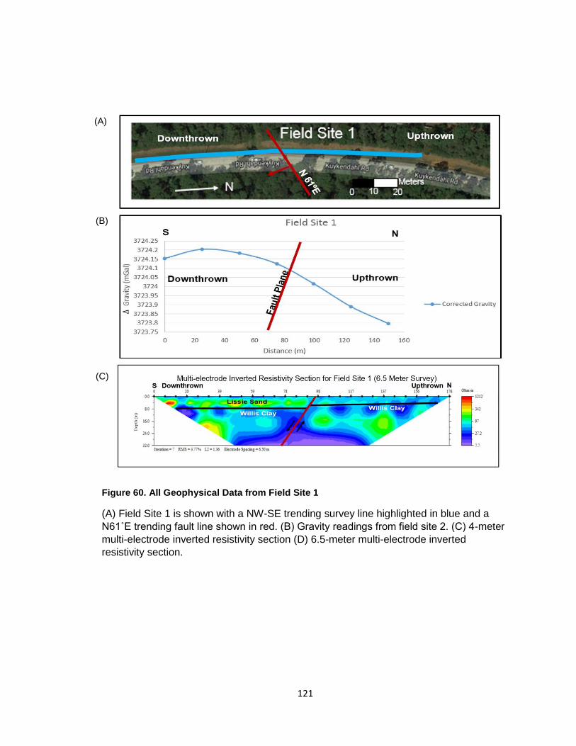
121
Figure 60. All Geophysical Data from Field Site 1
(A) Field Site 1 is shown with a NW-SE trending survey line highlighted in blue and a
N61˚E trending fault line shown in red. (B) Gravity readings from field site 2. (C) 4-meter
multi-electrode inverted resistivity section (D) 6.5-meter multi-electrode inverted
resistivity section.
(A)
(B)
(C)

122
Field Site 2
Field site 2 (Figure 61) utilized gravimetery, capacitively coupled resistivity and
multi-electrode resistivity techniques to delineate the faulting. Gravimetry readings from
field site 2 showed a higher gravity on the downthrown side of the fault and a lower
gravity on the upthrown side of the fault. Capacitively coupled resistivity readings were
displayed as an inverted resistivity section and had a total depth of 3.8 meters. The
capacitively coupled inverted resistivity section showed a higher accumulation of the
Lissie Sand on the downthrown side of the fault and a higher accumulation of the Willis
Clay on the upthrown side of the fault. The multi-electrode inverted resistivity section
showed the Lissie Sand in higher accumulation on the downthrown side of the fault and
the Willis Clay in higher accumulation on the upthrown side of the fault. The offset of the
layers was found to be 2 meters at this field site. A small accumulation of the Lissie
Sand was found in the center of the survey line and is reflected in the gravity data with
higher readings and in the multi-electrode inverted resistivity section with higher
resistivity readings.

123
Figure 61. All Geophysical Data from Field Site 2
(A) Survey site 2 with the NW-SE trending survey line highlighted in blue and a N58˚E trending
fault line highlighted in red. (B) Plotted gravimetry readings from field site 2 (C) CCR inverted
resistivity section (D) Multi-electrode inverted resistivity section.
3726.6
3726.7
3726.8
3726.9
0 20 40 60 80 100
Gra
vity
(m
Gal
)
Distance (m)
Gravity Data for Field Site 2
Stations
Downthrown Upthrown
(C)
(D)
(B)
(A)
6.5-Meter Multi-Electrode Inverted Resistivity Section for Field Site 2
Field Site 2

124
Field Site 3
Field Site 3 (Figure 62) utilized gravity and capacitively coupled resistivity
techniques to delineate the fault line. Plotted gravimetery readings from field site
3 showed higher gravity readings on the downthrown side of the fault and lower
gravity readings on the upthrown side of the fault. Capacitively coupled resistivity
section with the Lissie Sand found in higher accumulation on the downthrown
side of the fault and the Willis Clay in higher accumulation on the upthrown side
of the fault. The total depth of the capacitively coupled resistivity survey was 3.83
meters. The plotted gravimetery readings correlated well with the capacitively
coupled resistivity section for field site 3.

125
(B)
(A)
Figure 62. All Geophysical Data from Field Site 3
(A) Survey site 3 with the NW-SE trending survey line highlighted in blue and the N66˚E
trending fault line highlighted in red. (B) Gravimetry readings from field site 3. (C)
Capacitively-coupled inverted resistivity section.

126
Field Site 4
Field site 4 (Figure 63) only utilized gravimetry readings to
delineate the fault. Anthropogenic barriers such as busy roadways,
businesses and residences prevented any electrical resistivity techniques
to be used at this field site. Using gravimetry, it was determined that the
downthrown (southern) side of the fault had higher gravity readings than
the (northern) upthrown side of the fault. The denser Lissie Sand was
found to be in higher accumulation on the downthrown side of the fault
and the less dense Willis Clay was found in higher accumulation on the
upthrown side of the fault.

127
Figure 63. All Geophysical Data from Field Site 4
(A) Study area for field site 2 with the N54ºE trend of the fault line highlighted in red and
the survey line highlighted in blue. (B) Plotted gravimetery readings from field site 4.

128
Field Site 5
Field site 5 (Figure 64) utilized gravimetry and multi-electrode electrical
resistivity techniques to delineate the fault. The plotted gravimetry readings with
the upthrown side of the fault were found to have slightly lower gravity readings
than the upthrown side of the fault. The lowest gravity readings were found in the
center of the survey. The multi-electrode inverted resistivity section showed the
Lissie Sand being the upper lithologic unit and the Willis Clay lying conformably
underneath it. Normal faulting offset the Willis Clay and Lissie Sand by 2 meters.
The changes in gravity match the faulting patterns shown in the inverted
resistivity section. The anomalously low gravity readings at the center of the
survey corresponded well to the multi-electrode electrical resistivity inverted
resistivity section.
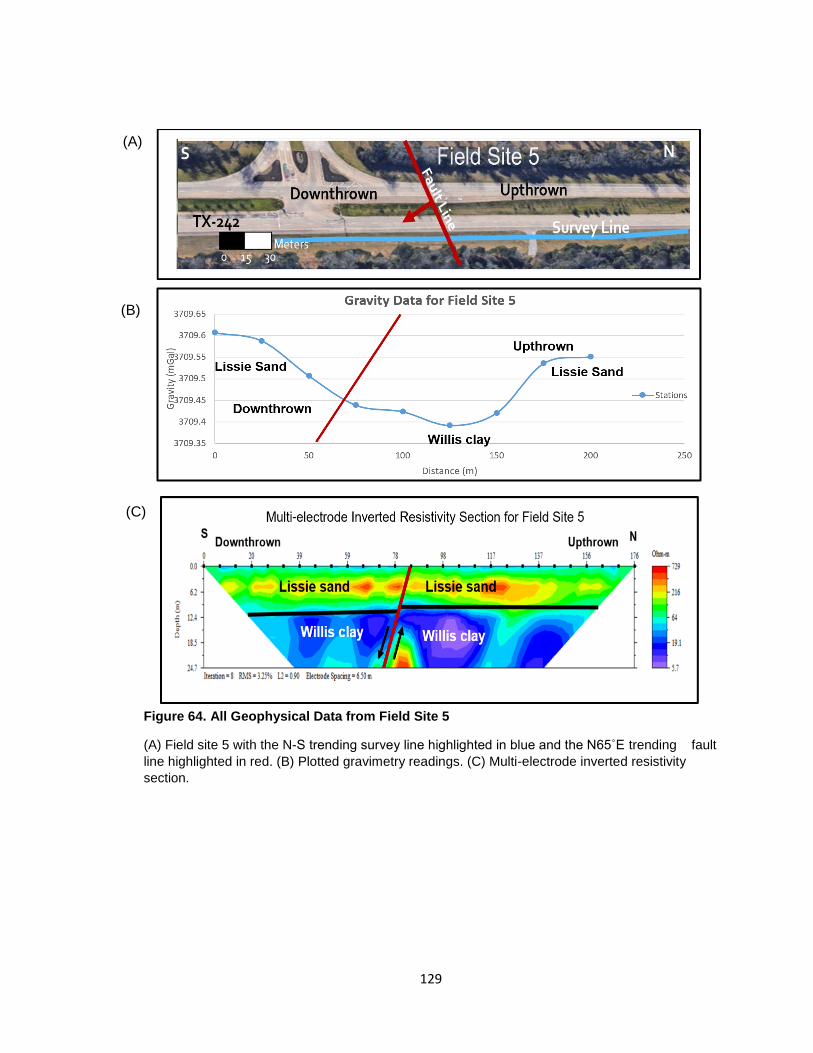
129
Figure 64. All Geophysical Data from Field Site 5
(A) Field site 5 with the N-S trending survey line highlighted in blue and the N65˚E trending fault
line highlighted in red. (B) Plotted gravimetry readings. (C) Multi-electrode inverted resistivity
section.
(B)
(A)
(C)

130
Field Site 6
Field site 6 (Figure 65) only utilized gravimetry techniques due to the field
site being located on the frontage road of Interstate Highway 45. Commercial
driveways intersected the prospective survey line so neither electrical resistivity
technique could be utilized. Using gravimetry techniques, it was determined that
the downthrown side of the fault had higher gravity readings than the upthrown
side of the fault. The denser Lissie Sand was found to be in higher accumulation
on the downthrown side of the fault and the less dense Willis Clay was found in
higher accumulation on the upthrown side of the fault. Anomalously high gravity
readings were found near the center of the survey, which is also where the
suspected fault line crossed the survey line. This anomaly could due to a higher
concentration of Lissie Sand near the fault plane, but further studies should be
done to confirm this.

131
Figure 65. All Geophysical Data from Field Site 6
(A) Study area for field site 6 with the N62ºE trend of the fault line highlighted in red and the
survey line highlighted in blue. (B) Plotted corrected gravity data from field site 6.
N S Gravity Readings from Field Site 6
132
Field Site 7
Field site 7 (Figure 66) utilized capacitively coupled electrical resistivity
techniques and multi-electrode resistivity techniques to delineate the fault.
Gravimetery techniques were not utilized at this field site due to equipment
malfunctions in the field. The capacitively coupled inverted resistivity section
showed higher resistivity Lissie Sand on the upthrown side of the fault and the
lower resistivity Beaumont Clay on the downthrown side of the fault. The depth of
the survey was 3.83 meters. The multi-electrode inverted resistivity section
corresponded well to this and showed the Beaumont Clay as the upper geologic
unit on the downthrown side of the fault and the Lissie Sand as the upper
geologic unit on the upthrown side of the fault. The fault was determined to be a
normal fault dipping toward the Gulf of Mexico. The Lissie Sand and Willis Clay
were offset at this field site by 5 meters. The depth of the survey was 42.5
meters.

133
(A)
(C)
Figure 66. All Geophysical Data from Field Site 7
(A) Field site 7 with the NW-SE trending survey line highlighted in blue and the N65˚E trending
fault line highlighted in red. (B) CCR inverted resistivity section (C) Multi-electrode inverted
resistivity section.
Beaumont Clay
(B)
(A)

134
CHAPTER 7
7.0 LIMITATIONS
The field sites for this study were all located in urban environments which
caused many challenges in conducting geophysical field work. Some field sites
were located on busy roadways, such as field site 6 which was located on the
frontage road of Interstate Highway 45. Field site 6 was limited to using
gravimetry techniques because of these anthropogenic barriers and problems
with gaining access to private properties. Capacitively coupled resistivity
techniques could only be used on three field sites because of anthropogenic
barriers such as woods or busy driveways The OhmMapper resistivity meter is a
very long apparatus that had to be pulled by the surveyor, which caused further
limitations in line length and survey location. The RMS error associated with
capacitively coupled resistivity techniques was higher than the multi-electrode
resistivity techniques which could have been caused by variance in the field
setup. Since the equipment for the capacitively coupled resistivity surveys were
being towed, any bump or depression in the roadways could have caused extra
noise in the survey.

135
7.1 CONCLUSION
For this study the Big Barn fault was examined using electrical resistivity
and gravimetry techniques. Seven field sites were examined in total and each
site used varying methodologies to delineate the fault and define the geology of
the upper rock units. All field sites showed significant fractures in roadways along
with a sharp contrast in elevation from the upthrown side of the fault to the
downthrown side. The N62ºE trending fault line was interpreted to trend along the
same strike as the intersection of the Lissie Sand and Willis Clay, in most cases.
Gravimetry techniques were first used to delineate the fault because of the
varying densities of the Lissie Sand and Willis Clay. The Lissie Sand was denser
than the Willis Clay, so it had higher gravity readings. The gravity data was
compared to the electrical resistivity data to determine the subsurface features in
each field sites. The capacitively coupled and multi-electrode electrical resistivity
data correlated well to the gravimetry data.
Field sites 1, 2, 5 and 7 showed a 2-5-meter offset between the
interpreted Lissie Sand and Willis Clay. Field site 2 was the only field site that
was able to utilize gravimetry, capacitively coupled resistivity and multi-electrode
resistivity techniques to delineate the Big Barn fault and identify other subsurface
features. All three geophysical techniques showed the Lissie Sand in higher
accumulation on the downthrown side of the fault and the Willis Clay in higher

136
accumulation on the upthrown side of the fault. This corresponds to the geologic
contact of the Lissie Sand and Willis Clay initially determined by previous
geologic mapping. This truncation could have been caused normal faulting
(Figure 4). Gravimetry and electrical resistivity data from the field sites correlated
well and defined a higher resistivity anomaly in the Willis Clay on the upthrown
side of the fault. Field sites 1 and 5 also showed an offset of the Lissie Sand and
the Willis Clay layers in the proximity of a normal fault. Field site 7 showed the
greatest offset of approximately 5m and showed a higher concentration of the
Lissie Sand on the downthrown side of the fault and the Willis Clay on the
upthrown side of the fault. For this field site another low resistivity layer was
found to be above the Lissie Sand on the downthrown side which could be
attributed to the field site’s close location to the East Fork of the San Jacinto
River. This layer was determined to be the Beaumont Clay. The USGS reported
the Beaumont Clay in the same area as field site 7, which could account for the
layer above the Lissie Sand.

137
7.2 FUTURE WORK
Future work could be done by utilizing more geophysical techniques along
the fault line. Field investigations for this survey were extended past the seven
field locations but anthropogenic barriers limited the extent of the study. More
extensive field mapping could be done to more precisely define where the Lissie
Sand truncates the Willis Clay and to determine the extent of the Beaumont Clay.
Further work could be completed by extending the length of the fault line to the
southwest and northeast.
Subsidence is a known problem in the Gulf Coastal Plain and could have
been caused by a variety of factors. Conducting subsidence studies through time
using LiDAR elevation maps could determine the reactivation of the fault line.
Saribudak et. al., 2018, used LiDAR elevation maps along with other geophysical
methods to further characterize the Hockley fault. Examining elevations in the
study area throughout time could be useful in determining the timing of faulting,
which could be correlated to a specific cause of reactivation. This timing could be
correlated to subsidence rates in the city of Houston, which could be caused by
anthropogenic or natural causes. To further prevent damages to residences,
businesses and roadways it is important that continuous studies be done on
faults throughout the greater Houston area to pinpoint the cause of reactivation of
faulting and to map the true extent of the fault lines.

138
REFERENCES
AGI, 2005. Instruction manual for the SuperSting with Swift automatic resistivity and IP
system: Austin, TX, Advanced Geosciences, Inc., 87 p. AGI, 2017. Seminar on resistivity imaging, AGI Resistivity Imaging Seminar, Nov. 6-8,
Austin, TX. Aronow, S., Fisher, W.L., McGowen, J.H., and Barnes, V.E. (V.E. Barnes, Project Director), 1982,
Geologic atlas of Texas, Houston sheet: Austin, University of Texas, Bureau of Economic
Geology, scale 1:250,000.
Baker, E.T., 1994, "Stratigraphic Nomenclature and Geologic Sections of the Gulf Coastal Plains
Barker, R. A., and Ardis, A. F., 1996, Hydrogeologic framework of the Edwards-Trinity Aquifer System, west-central Texas: U.S. Geological Survey Professional Paper 1421-B, 61 p.
with plates.of Texas" U.S. Geological Survey Open-File Report 94-461.
Ball, L., Kress, W., Steele, G., Cannia, J., and Andersen, M., 2004, Determination of canal
leakage potential using continuous resistivity profiling techniques, Interstate and Tri-State
Canals, Western Nebraska and Eastern Wyoming: U.S. Department of the Interior, U.S.
Geological Survey Open-File Report 2006-5032, p. 8.
Barton, D.C., Ritz, C., and Hickey, M., 1933, Gulf Coast geosyncline: Am. Assoc. Petroleum
Geologists Bull., v. 17, p. 1446-1458.
Bates, R.L., and Jackson, J.A., 1984, Dictionary of geologic terms: The American
Institute, Anchor Books, New York.
Bauer, P., 1999, The Gravity Geophysical Method, Astronaut Geophysical Training, New Mexico
Bureau of Geology and Mineral Resources, New Mexico Technical University,
https://geoinfo.nmt.edu/geoscience/projects/astronauts/gravity_method.html.
Bebout, D.G., Luttrell, P.E., and Seo, J.H., 1976, Regional Tertiary cross sections Texas Gulf
Coast: Austin, University of Texas, Bureau of Economic Geology Geological Circular 76-
5, 10 p.
Beckman, J.D. and Williamson, A.K., 1990, Salt-Dome Locations in the Gulf Coastal Plain, South-
Central United States, U.S. Geological survey water-Resources Investigations Report 90-
4060.

139
Berryhill, H.L., Jr., Suter, J.R., and Hardin, N.S., 1987, Late Quaternary Facies and Structure,
Northern Gulf of Mexico Interpretations from Seismic Data, American Association of
Petroleum Geologists Studies in Geology no. 23, 289 p.
Billings, M.P., 197, Structural Geology, 3rd Edition, London, Prentice-Hall International, Inc,
ISBN: 0-13-853846-8, print.
Bird, D., Burke, K., Hall, S., and Casey, J., 2005, Gulf of Mexico Tectonic History: Hotspot Tracks,
Crustal Boundaries, and Early Salt Distribution, American Association of Petroleum
Geologists Bulletin, v. 89, p. 311–328, doi: 10.1306/10280404026.
Blakey, R., 2016, Paleogeography and Geologic Evolution of North America:
www.jan.ucc.nau.edu/rcb7/nam.html. Accessed April, 10 2016.
Braile, L.W., Hinze W.J., Geller G.R., Lidiak E.G., and Sexton J.L., 1986 Tectonic Development of the New Madrid Rift Complex, Mississippi Embayment, North America,
Tectonophysics, 131, p. 1-21. Brun, J., and Mauduit, T., Rollovers in salt tectonics: The inadequacy of the listric fault model, 2008, Tectonophysics, 457, p. 1-11.
Bureau of Economic Geology., 1992, Geology of Texas, University of Texas at Austin, 2 p.
Byerly, G.R., 1991, Igneous activity, in Salvador, A., editor, The Gulf of Mexico Basin: Boulder, Colorado, Geological Society of America, The Geology of North America, v. J., p. 91-108.
Cardimona, S., 2002, Electrical resistivity techniques for subsurface investigation: Department of
Geology and Geophysics, University of Missouri Rolla, Rolla, MO, p. 1-10.
Carpenter, P.J., 1997, Use of resistivity and EM Techniques to Map Subsidence Fractures in
Glacial Drift, Association of Environmental and Engineering Geologists, v. 8, doi:
10.2113/gseegeosci.III.4.523.
Campbell, M.D., Wise, H.M., and Bost, R.C., 2015, Growth Faulting and Subsidence in the
Houston, Texas Area: Guide to the Origins, Relationships, Hazards, Potential Impacts
and Methods of Investigation, Institute of Environmental Technology, Technical Report,
doi: 10.13140.
Chowdhury, A.H., Boghici, R., and and Hopkins, J., 2006, Hydrochemistry, Salinity Distribution,
and Trace Constituents: Implications for Salinity Sources, Geochemical Evolution, and
Flow Systems Characterization, Gulf Coast Aquifer, Texas. Texas Water Development
Board, Report R365, ch. 5.

140
Doering, J., “Post Fleming Surface Formations of Coastal Southeast Texas and South Louisiana,
Bulletin of the North American Association of Petroleum Geologists, Vol. 19. No. 5 (May,
1935), p. 651-688.
Engelkemeir, R.E., and Khan, S.D., 2007, Near surface geophysical studies of Houston faults:
The Leading Edge, v. 26, no. 8, p. 1004–1008, doi: 10.1190/1.2769557.
Engelkemeir, R., S. Khan, and Kevin Burke, 2010, Surface Deformation in Houston, Texas using
GPS, Tectonophysics, Vol. 490, p. 47–54.
Ferrill, D.A., Morris, A., 2008, Fault Zone Deformation Controlled by Carbonate Mechanical
Stratigraphy, Balcones Fault System, Texas, AAPG Bulletin 92(3):359-380.
Fugro Consultants, Inc., 2012, Geologic Fault Delineation Study SJRA Distribution Lines, Route
W1, San Jacinto River Authority, Montgomery County, Texas.
Garrison, L.E., and Martin, R.G., Jr., 1973, Geologic structures in the Gulf of Mexico basin: U.S.
Geological Survey Professional Paper 773, 85 p.
Geometrics, Geophysical Methods, Capacitively Coupled Resistivity,
http://www.geometrics.com/applications/geophysical-methods/capacitively-coupled-
resistivity/.
Halbouty, M. T., 1967, Salt Domes, Gulf Coast region, United States and Mexico: Gulf Publishing
Company, Houston, Texas, 425 p.
Hatherton, T., and Hunt, T.M., 1968, Gravity Profiles across the Alpine Fault, New Zealand,
Journal of Geophysical Research, Vol. 73, No. 16, August 15, 1968.
Hentz, T.F., and Zeng, H., 2003, High-frequency Miocene sequence stratigraphy, offshore
Louisiana: Cycle framework and influence on production distribution in a mature shelf
province, AAPG Bulletin, v. 87, no. 2 (February 2003), p. 197–230.
Hosman, R.L., 1996, "Regional Stratigraphy and Subsurface Geology of Cenozoic Deposits, Gulf
Coastal Plain, South-Central United States" U.S. Geological Survey Professional Paper
1416-G.
Hosman, R.L. and Weiss, J.S., 1991, Geohydrologic units of the Mississippi Embayment and Texas Coastal Uplands Aquifer Systems, South-Central United States – Regional aquifer system analysis-G.
Hudec, M. R., Norton N. O., Jackson, M. P. A., and Peel F. J., 2013, Jurassic evolution of the Gulf of Mexico salt basin: AAPG Bulletin, 97, p. 1683–1710, doi: 10.1306/04011312073. Jackson, M.P.A., 1982, Fault tectonics of the East Texas Basin: Texas Bureau of Economic Geology, Geologic Circular 82-4, Austin, p. 31.

141
Khan, S.D., Stewart, R.R., Otoum, M., et. al., 2013, A geophysical investigation of the active
Hockley Fault System near Houston, Texas, Geophysics, Vol. 78, No. 4, pp. B177-B185.
Kneller, E. A., and C. A. Johnson, 2011, Plate kinematics of the Gulf of Mexico based on integrated observations from the Central and South Atlantic: Gulf Coast Association of Geological Societies Transactions, 61, p. 283–299. Kolay, K.K., Sandeep, B.G., and Sanjeev, K. 2016, Effect of Salt and NAPL on electrical
resistivity of fine-grained soil-sand mixtures: International Journal of Geotechnical
Engineering, pp. 1-7, doi:10.1080/19386362.2016.1239378.
Loke, M.H.,1999, Electrical imaging surveys for environmental and engineering studies: A practical guide to 2-D and 3-D surveys. 63 p.
Lowrie, W., 2007, Fundamentals of Geophysics, Second Edition: Cambridge University Press.
Marton, G., and R. T. Buffler, 1994, Comment on Jurassic reconstruction of the Gulf of Mexico Basin: International Geology Review, 36, p. 545–586, doi: 10.1080/00206819409465475. Majzoub, A.F., 2016, Characterization and Delineation of Karst Geohazards Along RM652 Using Electrical Resistivity Tomography, Culberson County, Texas, Stephen F. Austin State University, Electronic Theses and Dissertations.
McGookey, D.P., 1975, Gulf Coast Cenozoic sediments and structure: An excellent
example of extra-continental sedimentation: Gulf Coast Association of Geological Societies Transactions, v. 25, p. 104-120.
Metcalf, R.J., “Deposition of Lissie and Beaumont Formations of Gulf Coast of Texas”, Bulletin of the American Association of Petroleum Geologists, Vol. 24, No. 4 (April, 1940), p. 693-700. Moore, D.W. and Wermund, E.G., Jr., 1993a, Quaternary geologic map of the Austin 4 x 6 degree quadrangle, United States: U.S. Geological Survey Miscellaneous Investigations Series Map I-1420 (NH-14), scale 1:1,000,000. Mussett, A.E., and Khan, A.M., 2000, Looking into the earth: An introduction to
geological geophysics: Cambridge, Cambridge University Press. Norman, C. E., and Britt, P.W., 1991, Active Faults in North Harris County and South Central Montgomery County, Texas, in Environmental and Engineering Geology of North Harris and South Montgomery Counties, Texas, Houston Geological Society Guidebook 91-1, Field Trip of October 19, p. 13-27. Norman, C.E., 2005, Ground subsidence and active faults in the Houston metropolitan area: Coastal subsidence, sea level and the future of the Gulf Coast: Houston Geological Society/Engineering, Science and Technology Council of Houston Conference, Field Trip Guide.

142
Nguyen, L.C., and Mann, P., 2016, Gravity and magnetic constraints on the Jurassic opening of the oceanic Gulf of Mexico and the location and tectonic history of the Western Main transform fault along the eastern continental margin of Mexico, Interpretation, Vol. 4, No. 1 (February 2016); p. SC23–SC33. Okocha, F.C., 2016, Gravitational Study of the Hastings Salt Dome and Associated Faults in Brazoria and Galveston Counties, Texas, Master’s thesis, Stephen F. Austin State University, http://scholarworks.sfasu.edu/etds/80. Oldani, M.J., 1986, Episodic Sedimentation in the Rio-Grande-Trans Pecos Region as Related to Periods of Tectonic Activity, Houston Geological Society, Field Seminar of the Big Bend, Trans-Pecos Region, Texas. Pindell, J. L., andKennan L., 2009, Tectonic evolution of the Gulf of Mexico, Caribbean and northern South America in the mantle reference frame: An update, in K. H. James, M. A. Lorente, and J. L. Pindell, eds., SC32 Interpretation / February 2016, the origin and evolution of the Caribbean Plate: Geological Society of London, 1–5. Pratsch, J.C., 1997 Relationship of Gulf Coast Basement Tectonics to Present and Future Oil and
Gas Fields, Houston Geological Society, June 1997 Issue.
Rucker, D.F., Noonan, G.E., and Greenwood, W.J., 2011, Electrical resistivity in support of
geological mapping along the Panama Canal, Engineering Geology 117, p. 121-133.
Saribudak, M., 2011, Geophysical mapping of the Hockley growth fault in northwest Houston,
USA, and recent surface observations, the Leading Edge, Near-Surface Geophysics, p.
936-943.
Saribudak, M., Ruder, M., and Nieuwenhuise, B.V., 2018, Hockley Fault revisited: More
geophysical data and new evidence on the fault location, Houston, Texas, Geophysics,
Vol. 83, No.3, p. 1-10.
Scintrex, 2008, CG-5 Scintrex Autograv System Operation Manual, part # 867700 Revision 5.
Scintrex, 2012, www.scintrexltd.com [Retrieved December, 2017].
Solis, , R.F., “Upper Tertiary and Quaternary Depositional Systems, Central Coastal Plain, Soli
Texas”, 1981, Bureau of Economic Geology, Report of Investigations, No. 108.
Stoneham, S. L., 1953, A Generalized Geologic North-South Cross Section from Hays County,
Texas, to the Gulf of Mexico, Guidebook, A.A.P.G. Annual Meeting, Houston, Texas
(March), p. 24-25.
USGS, 2018, Geologic Units of Montgomery County, https://mrdata.usgs.gov/geology/state/fips-
unit.php?code=f48339. [Retrieved January 2018].
Telford, W.M., Geldart, L.P., and Sheriff, R.E., Applied Geophysics, Second Edition: Cambridge, Cambridge University Press, 1990.

143
Thomas, W. A., 2011, The Iapetan rifted margin of southern Laurentia, Geosphere, vol. 7, p. 97-
120.
Thompson, W.C., 1937, Geologic sections in Texas and adjoining states: American Association
of Petroleum Geologists Bulletin, v. 21, no. 8, p. 1,083-1,087.
Trimble Inc., 2011, NOMAD 9000 Series Users Guide: www.Trimble.com [Accessed January,
2018].
Van Siclen, D. C., 1967, The Houston fault problem: American Institute of Professional
Geologists, Texas Section: Third Annual Meeting Proceedings, p. 9–31.
Verbeek, E. R., 1978, Quaternary fault activity in Texas Gulf Coast: American Association of
Petroleum Geologists Bulletin, v. 63, p. 545–545.
Verbeek, E. R., and Clanton U. S., 1981, historically active faults in the n
metropolitan area, Texas, Houston area environmental geology, in E. M. Etter, ed.,
Houston area environmental geology: Surface faulting, ground subsidence, and hazard
liability: Houston Geological Society, Texas, p. 28–68.
Wada, S., Sawada, A., Hiramatsu, Y., et. al., 2017, Continuity of subsurface fault structure
revealed by gravity anomaly: the eastern boundary fault zone of the Niigata plain, central
Japan, Earth, Planets and Space, 69:15, doi: 10.1186/s40623-017-0602-x.
Waters, P. W. McFarland, and J. W. Lea, 1955, Geologic Framework of Gulf Coastal Plain of
Texas, Bulletin, A.A.P.G. Vol. 39. NO. 9 (September, 1955). p. 1821-1850.
Williamson, J.D.M., 1959, Gulf Coast Cenozoic history: Gulf Coast Association of Geological
Societies Transactions, v. 9, p. 15-29.
Winker, C.D., 1982, Cenozoic shelf margins, northwestern Gulf of Mexico: Gulf Coast Association
of Geological Societies Transactions, v.32, p.427 – 448.
Wood, D.H. and Giles, A.B., 1982, Hydrocarbon Accumulation Patterns in the East Texas Salt
Dome Province, Bureau of Economic Geology, Geological Circular, 82-6.
Woodruff, C.M. Jr., 1980, Regional Tectonic Features of the Inner Gulf Coast Basin and the
Mississippi Embayment, Gulf Coast Associations of Geologic Societies.
Yamashita, Y., Groom, D., Inazaki, T., and Hayashi, K., 2004, Rapid near surface resistivity
survey using the capacitively-coupled resistivity system: OhmMapper, OYO Corporation,
Japan, Geometrics, Public Works Research Institute, Japan.
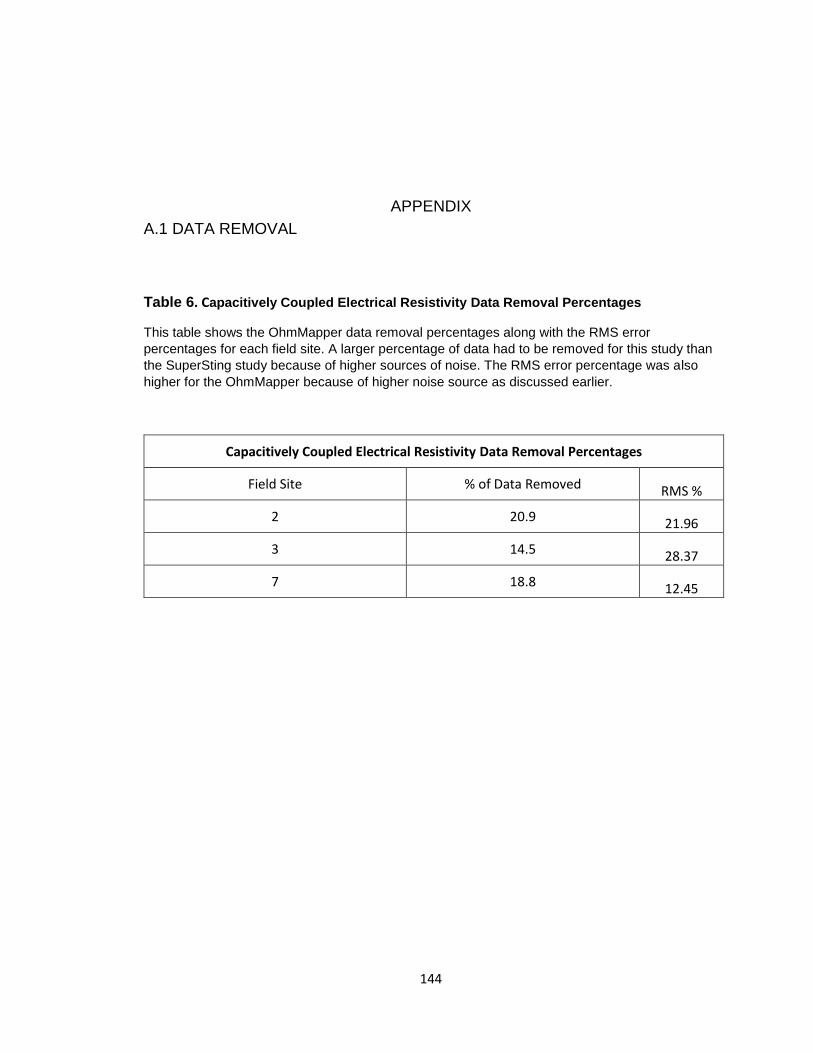
144
APPENDIX
A.1 DATA REMOVAL
Table 6. Capacitively Coupled Electrical Resistivity Data Removal Percentages
This table shows the OhmMapper data removal percentages along with the RMS error
percentages for each field site. A larger percentage of data had to be removed for this study than
the SuperSting study because of higher sources of noise. The RMS error percentage was also
higher for the OhmMapper because of higher noise source as discussed earlier.
Capacitively Coupled Electrical Resistivity Data Removal Percentages
Field Site % of Data Removed RMS %
2 20.9 21.96
3 14.5 28.37
7 18.8 12.45

145
Table 7. Multi-Electrode Electrical Resistivity Removal Percentages
This table shows the percentage of data removed from each field site for all multi-electrode
electrical resistivity surveys. The RMS (Root Mean Squared) percentage is also shown for each
field site. The maximum amount of data removed at any field site was 14.3% while the highest
RMS was found to be 9.93%.
Multi-Electrode Electrical Resistivity Removal Percentages
Field Site % of Data Removed RMS %
1 (6.5m) 8.1 3.77
2 (4.0m) 10.1 3.34
2 (6.5m) 11.3 5.69
5 (6.5m) 5.6 3.25
7 (6.5m) 14.3 9.93
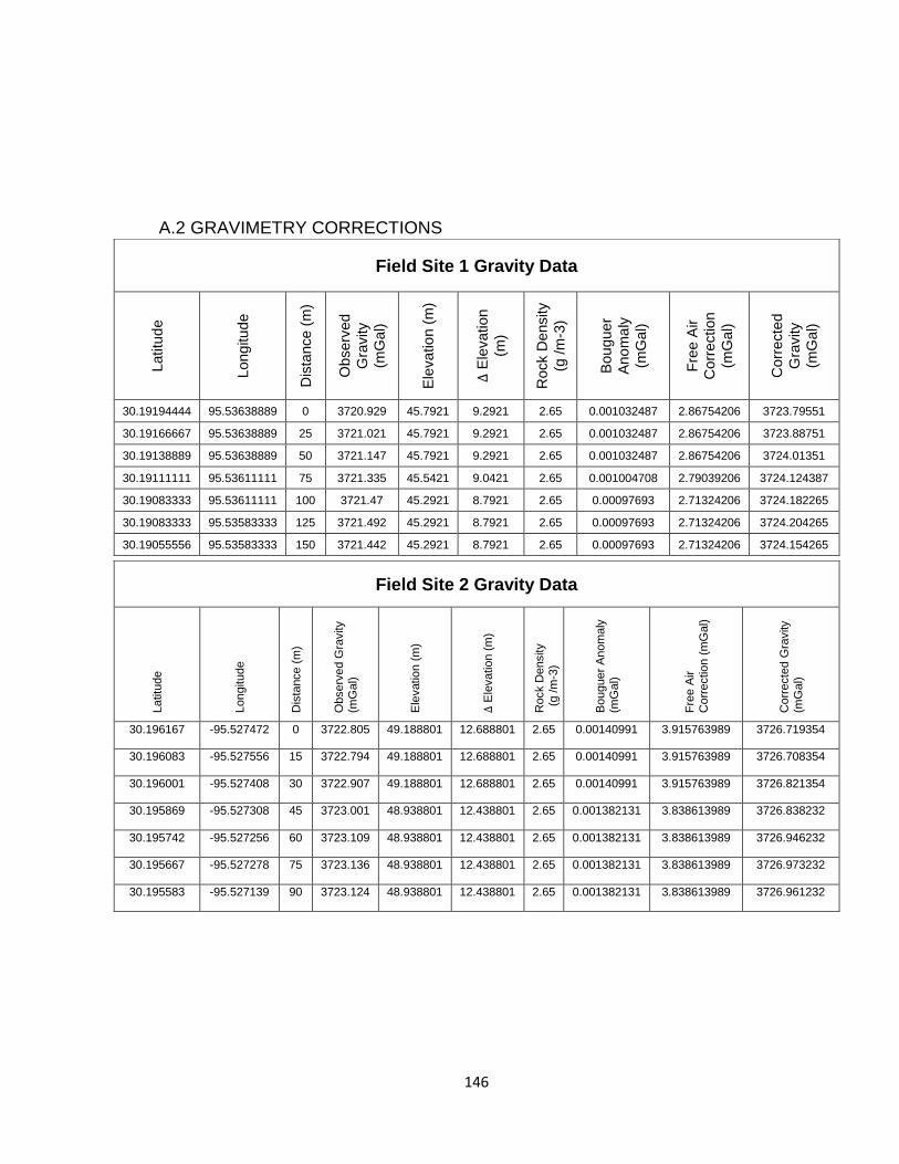
146
A.2 GRAVIMETRY CORRECTIONS
Field Site 1 Gravity Data
Latitu
de
Long
itu
de
Dis
tance (
m)
Observ
ed
Gra
vity
(mG
al)
Ele
va
tio
n (
m)
∆ E
levation
(m)
Rock D
ensity
(g /m
-3)
Bou
guer
Ano
ma
ly
(mG
al)
Fre
e A
ir
Corr
ection
(mG
al)
Corr
ecte
d
Gra
vity
(mG
al)
30.19194444 95.53638889 0 3720.929 45.7921 9.2921 2.65 0.001032487 2.86754206 3723.79551
30.19166667 95.53638889 25 3721.021 45.7921 9.2921 2.65 0.001032487 2.86754206 3723.88751
30.19138889 95.53638889 50 3721.147 45.7921 9.2921 2.65 0.001032487 2.86754206 3724.01351
30.19111111 95.53611111 75 3721.335 45.5421 9.0421 2.65 0.001004708 2.79039206 3724.124387
30.19083333 95.53611111 100 3721.47 45.2921 8.7921 2.65 0.00097693 2.71324206 3724.182265
30.19083333 95.53583333 125 3721.492 45.2921 8.7921 2.65 0.00097693 2.71324206 3724.204265
30.19055556 95.53583333 150 3721.442 45.2921 8.7921 2.65 0.00097693 2.71324206 3724.154265
Field Site 2 Gravity Data
Latitu
de
Longitude
Dis
tance (
m)
Observ
ed G
ravity
(mG
al)
Ele
vatio
n (
m)
∆ E
levatio
n (
m)
Rock D
ensity
(g /m
-3)
Bouguer
Anom
aly
(m
Ga
l)
Fre
e A
ir
Corr
ectio
n (
mG
al)
Corr
ecte
d G
ravity
(mG
al)
30.196167 -95.527472 0 3722.805 49.188801 12.688801 2.65 0.00140991 3.915763989 3726.719354
30.196083 -95.527556 15 3722.794 49.188801 12.688801 2.65 0.00140991 3.915763989 3726.708354
30.196001 -95.527408 30 3722.907 49.188801 12.688801 2.65 0.00140991 3.915763989 3726.821354
30.195869 -95.527308 45 3723.001 48.938801 12.438801 2.65 0.001382131 3.838613989 3726.838232
30.195742 -95.527256 60 3723.109 48.938801 12.438801 2.65 0.001382131 3.838613989 3726.946232
30.195667 -95.527278 75 3723.136 48.938801 12.438801 2.65 0.001382131 3.838613989 3726.973232
30.195583 -95.527139 90 3723.124 48.938801 12.438801 2.65 0.001382131 3.838613989 3726.961232

147
Field Site 3 Gravity Data
Latitu
de
Longitude
Dis
tance (
m)
Observ
ed G
ravity
(mG
al)
Ele
vatio
n (
m)
∆ E
levatio
n (
m)
Rock D
ensity
(g /m
-3)
Bouguer
Anom
aly
(m
Ga
l)
Fre
e A
ir
Corr
ectio
n (
mG
al)
Corr
ecte
d G
ravity
(mG
al)
30.201053 -95.519806 0 3693.38 49.624363 13.124363 2.65 0.001458307 4.050178422 3697.42872
30.200647 -95.519606 25 3693.398 49.624363 13.124363 2.65 0.001458307 4.050178422 3697.44672
30.200583 -95.519556 50 3693.506 49.624363 13.124363 2.65 0.001458307 4.050178422 3697.55472
30.200442 -95.519403 75 3693.74 49.124363 12.624363 2.65 0.00140275 3.895878422 3697.634476
30.200269 -95.519403 100 3693.82 48.874363 12.374363 2.65 0.001374971 3.818728422 3697.637353
30.200106 -95.519228 125 3693.897 48.874363 12.374363 2.65 0.001374971 3.818728422 3697.714353
30.199925 -95.519069 150 3693.825 48.874363 12.374363 2.65 0.001374971 3.818728422 3697.642353

148
Field Site 5 Gravity Data
Latitu
de
Longitude
Dis
tance (
m)
Observ
ed G
ravity
(mG
al)
Ele
vatio
n (
m)
∆ E
levatio
n (
m)
Rock D
ensity
(g
/m
-3)
Bouguer
Anom
aly
(mG
al)
Fre
e A
ir
Corr
ectio
n (
mG
al)
Corr
ecte
d G
ravity
(mG
al)
30.211833 -95.501011 0 3704.229 53.752323 17.252323 2.65 0.001916983 5.324066878 3709.55115
30.211639 -95.500806 25 3704.214 53.750323 17.250323 2.65 0.001916761 5.323449678 3709.535533
30.211417 -95.500761 50 3704.176 53.500313 17.000313 2.65 0.001888981 5.246296592 3709.420408
30.211253 -95.500667 75 3704.147 53.500313 17.000313 2.65 0.001888981 5.246296592 3709.391408
30.211056 -95.500572 100 3704.256 53.250313 16.750313 2.65 0.001861203 5.169146592 3709.423285
30.210917 -95.500406 125 3704.333 53.050313 16.550313 2.65 0.00183898 5.107426592 3709.438588
30.210694 -95.500344 150 3704.402 53.048313 16.548313 2.65 0.001838758 5.106809392 3709.506971
Field Site 6 Gravity Data
Latitu
de
Longitude
Dis
tance (
m)
Observ
ed G
ravity
(mG
al)
Ele
vatio
n (
m)
∆ E
levatio
n (
m)
Rock D
ensity
(g
/m
-3)
Bouguer
Anom
aly
(mG
al)
Fre
e A
ir
Corr
ectio
n (
mG
al)
Corr
ecte
d G
ravity
(mG
al)
30.229975 -95.457725 0 3722.55 39.047815 2.547815 2.65 0.000283032 0.786255709 3723.335973
30.229850 -95.457694 20 3722.596 39.045315 2.545315 2.65 0.000282754 0.785484209 3723.381201
30.229611 -95.457669 50 3722.708 39.020315 2.520315 2.65 0.000279977 0.777769209 3723.485489
30.229386 -95.457667 75 3722.809 39.017815 2.517815 2.65 0.000279699 0.776997709 3723.585718
30.229197 -95.457667 100 3722.828 38.517815 2.017815 2.65 0.000224155 0.622697709 3723.450474
30.228972 -95.457611 125 3722.865 38.267815 1.767815 2.65 0.000196383 0.545547709 3723.410351
30.228775 -95.457583 150 3722.872 38.242815 1.742815 2.65 0.000193606 0.537832709 3723.409639

149
A.3 CROSSPLOT OF MEASURED VS APPARENT RESISTIVITY
Figure 67. Crossplot of Measured vs. Apparent Resistivity from CCR Survey Site 2

150
Figure 68. Crossplot of Measured vs. Apparent Resistivity from CCR Survey Site 3
Figure 69. Crossplot of Measured vs. Apparent Resistivity from CCR Survey Site 7
Multi-electrode Resistivity Data Crossplot

151
Figure 70. Crossplot of Measured vs. Apparent Resistivity from Multi-electrode Resistivity Survey Site 1
Figure 71. Crossplot of Measured vs. Apparent Resistivity from Multi-electrode Resistivity
Survey Site 2
Figure 72. Crossplot of Measured vs Predicted Apparent Resistivity from Multi-electrode Resistivity Field Site 5

152
Figure 73. Crossplot of Measured vs Predicted Apparent Resistivity from Multi-electrode Resistivity Field Site 7

153
VITA
After graduating from Klein Collins High School, Spring, TX, in 2011,
Danielle Minteer entered Stephen F. Austin State University in Nacogdoches, TX.
She received the degree of Bachelor of Science from Stephen F. Austin State
University in August, 2016. In January 2017, she entered the Graduate School of
Stephen F. Austin State University, and received the degree of Master of Science
in May of 2018.
Permanent Address: 523 Willow Wisp Circle Spring, TX 77388
Style manual designation: Geological Society of America
This thesis was typed by Danielle R. Minteer