a generalized system dynamics model for managing
TRANSCRIPT

A Generalized System Dynamics Model for Managing Transition-Phases in Healthcare
Environments
By
Javier Calvo-Amodio, M.Sc. BM, BS ISE
A Dissertation
In
SYSTEMS AND ENGINEERING MANAGEMENT
Submitted to the Graduate Faculty
of Texas Tech University in
Partial Fulfillment of
the Requirements for
the Degree of
DOCTOR OF PHILOSOPHY
Approved
Patrick Patterson, Ph.D., P.E.
Chairperson of the Committee
Milton L. Smith, Ph.D.
Co-Chairperson of the Committee
James R. Burns Ph.D.
William J. Conover Ph.D.
David A. Wyrick, Ph.D., P.E.
Dominic Cassadonte
Interim Dean of the Graduate School
December, 2012

Copyright 2012, Javier Calvo-Amodio

Texas Tech University, Javier Calvo Amodio, December 2012
ii
ACKNOWLEDGMENTS
I am deeply thankful for those who stood by me throughout this long journey that
culminates with this dissertation. Ma, Ana, thanks for your understanding and
unconditional love and support.
I am very grateful to everyone who helped develop and complete this dissertation. The
following is a list of who I am in debt:
Dr. Patrick Patterson and Dr. Milton Smith for their guidance and trust.
Drs. James Burns, Jay Conover, and David Wyrick for their valuable insights.
Joe Mays, Michael Sullivan, Brent Magers and Dr. Pat Conover for their
unconditional support, time and insight.
Dr. Simon Hsiang and Ganapathy Natarajan for their invaluable support.
The Department of Industrial Engineering, Graduate School, Waterman Mexican-
American Scholarship and CONACYT for their financial support.
‘
To Ean.

Texas Tech University, Javier Calvo Amodio, December 2012
iii
TABLE OF CONTENTS
ACKNOWLEDGEMENTS……………………………………………………...ii
ABSTRACT…………………………………………………………………..ix
LIST OF TABLES……………………………………………………………..x
LIST OF FIGURES….………………………………………………………...xi
I. INTRODUCTION ........................................................................................... 1
History and Background ...................................................................................... 1
Problem Statement ............................................................................................... 4 Research Questions .............................................................................................. 5
First Research Question................................................................................................ 6 Second Research Question (Experiment 1) .................................................................. 6 Third Research Question (Experiment 2) ..................................................................... 7
Tasks .................................................................................................................... 8 Task 1: .......................................................................................................................... 8 Task 2: .......................................................................................................................... 8 Task 3: .......................................................................................................................... 8
Hypotheses ........................................................................................................... 8 General hypothesis for Experiment 1: .......................................................................... 8 General hypothesis for Experiment 2: .......................................................................... 9
Research Purpose ................................................................................................. 9 Theoretical Purpose ...................................................................................................... 9 Practical Purpose ........................................................................................................ 10
Research Objectives ........................................................................................... 11
Limitations ......................................................................................................... 11 Assumptions ....................................................................................................... 12
Relevance of this Study ..................................................................................... 12 Need for this Research ............................................................................................... 12 Benefits of this Research ............................................................................................ 13
Research Outputs and Outcomes ....................................................................... 13
II. LITERATURE REVIEW ..............................................................................15
Introduction ........................................................................................................ 15 Primary Theories and Historical Background .................................................... 15
Industrial engineering and engineering management tools in healthcare ................... 15 Lean in healthcare ............................................................................................................ 16

Texas Tech University, Javier Calvo Amodio, December 2012
iv
Complementary use of methodologies with lean thinking ......................................... 17 Lean Six Sigma .................................................................................................................. 18 Socio-technical systems - lean thinking ............................................................................ 20
Action Research ......................................................................................................... 20 Learning Curve ........................................................................................................... 21
Basics of Learning Curve ................................................................................................. 21 Relevant learning curve theory to this research work ...................................................... 21 Adaptation Function Learning Model .............................................................................. 23 Knowledge Production as a Control Variable .................................................................. 25
Learning Loop Model ................................................................................................. 26 Learning Curves and System dynamics ..................................................................... 27 Systems Thinking ....................................................................................................... 28 Critical Systems Thinking .......................................................................................... 29 System dynamics ........................................................................................................ 29
Causal loop diagrams as mental models .......................................................................... 32 Efficiency, efficacy, and effectiveness of a model ............................................................. 32 Model Validity in a System dynamics Model .................................................................... 34 System dynamics in healthcare ......................................................................................... 37
Electronic Health Records (EHR) .............................................................................. 37 Complementarist Approach ........................................................................................ 39
Theoretical Model .............................................................................................. 40
III. METHODOLOGY .......................................................................................49
Introduction ........................................................................................................ 49 Rationale ............................................................................................................ 49
Research Design................................................................................................. 49 Type of Research ........................................................................................................ 51 Research Focus ........................................................................................................... 52 Research Hypotheses Restated ................................................................................... 52
Tasks ................................................................................................................................. 53 Hypotheses ........................................................................................................................ 53
General hypothesis for Experiment 1: ........................................................................ 54 General hypothesis for Experiment 2: ........................................................................ 54
Collection and Treatment of Data ...................................................................... 56 Data Collection ........................................................................................................... 56
Quantitative Data ............................................................................................................. 56 Qualitative Data ............................................................................................................... 56
Simulation .................................................................................................................. 56 Case Study .................................................................................................................. 57 Treatment of Data ....................................................................................................... 57
Methodological Issues ....................................................................................... 57 Reliability ................................................................................................................... 57 Validity ....................................................................................................................... 58

Texas Tech University, Javier Calvo Amodio, December 2012
v
Replicability ............................................................................................................... 59 Bias ............................................................................................................................. 59 Representativeness ..................................................................................................... 60
Research Constraints .......................................................................................... 60 Model Development, and Validation ................................................................. 60
IV. A PROPOSED CONCEPTUAL SYSTEM DYNAMICS MODEL FOR MANAGING
TRANSITION-PHASES IN HEALTHCARE ENVIRONMENTS ........................62
Abstract .............................................................................................................. 62 Introduction. ....................................................................................................... 62 Background ........................................................................................................ 63
Methodology ...................................................................................................... 66 Adaptation Function. .................................................................................................. 66 System Dynamics. ...................................................................................................... 67
Operational Definitions ...................................................................................... 67 Problem Context. .............................................................................................................. 67 Generalized Model. ........................................................................................................... 68 Transition-Phase Management. ........................................................................................ 68
Transition-Phase Management Model (TPMM) ................................................ 68 Exploratory Study .............................................................................................. 71 Conclusions ........................................................................................................ 74
References. ......................................................................................................... 74
V. A GENERALIZED SYSTEM DYNAMICS MODEL FOR MANAGING
TRANSITION-PHASES IN HEALTHCARE ENVIRONMENTS ........................76
Abstract .............................................................................................................. 76
Introduction ........................................................................................................ 76 Systems Thinking ....................................................................................................... 78 Critical Systems Thinking .......................................................................................... 79 System dynamics ........................................................................................................ 79
Causal loop diagrams as mental models .......................................................................... 83 Efficiency, efficacy, and effectiveness of a model ............................................................. 83 Model Validity in a System dynamics Model .................................................................... 85
Learning Curve Theory ...................................................................................... 87 Relevant learning curve theory to this research work ................................................ 88 Adaptation Function Learning Model ........................................................................ 90
Efficiency of the Process ................................................................................... 96
Process rate of adaptation .................................................................................. 97 Unintended consequences (or damping factors) ................................................ 97 Research Question ............................................................................................. 97 Model Development – System Identification .................................................... 97
Efficiency of the Process substructure (a) .................................................................. 98
Texas Tech University, Javier Calvo Amodio, December 2012
vi
Adequacy of Technology in Company ............................................................................... 99 Adequacy of Technology for Project ................................................................................. 99 Training Frequency ........................................................................................................ 100 Training Duration ........................................................................................................... 100 Business Seasonality ....................................................................................................... 100 Organizational Culture ................................................................................................... 100 Maximum delay expected ................................................................................................ 100
Process Rate of Adaptation substructure (µ) ............................................................ 101 Feedback Turnover Time ................................................................................................ 102 Implementation Team Effectiveness ................................................................................ 102 Staff Learning Rate ......................................................................................................... 102 Communication Skills ..................................................................................................... 102 Staff Experience .............................................................................................................. 102 Staff Educational Level ................................................................................................... 103 Feedback Turnover Time ................................................................................................ 103
Damping Factors Sub-Structure ............................................................................... 103 Forgetting ....................................................................................................................... 104 Existence of SOPs (Standard Operating Procedures) .................................................... 104
Model Validation - Simulation ........................................................................ 104 Extremes tests ........................................................................................................... 105 Substructures effect on Qt......................................................................................... 110 Bias analysis ............................................................................................................. 113
Conclusions ...................................................................................................... 119 Dampened Oscillation .............................................................................................. 119 Path Forecasting ....................................................................................................... 119 Effects of the substructures on the percentage of errors per day .............................. 120 Model behavior in pessimistic, moderate and optimistic scenarios ......................... 120
Future Work ..................................................................................................... 121
VI. APPLICATION OF TRANSITION-PHASE MANAGEMENT MODEL IN
BILLING HEALTHCARE ENVIRONMENT ................................................123
Abstract ............................................................................................................ 123
Introduction ...................................................................................................... 123 Background ...................................................................................................... 123 Action Research ............................................................................................... 125
Problem Context .............................................................................................. 125 Data Collection Procedure ........................................................................................ 126
Long-term multi-phase project ........................................................................ 131
Conclusions ...................................................................................................... 134 Future Work ..................................................................................................... 135
Forecasting capabilities ............................................................................................ 135 Further investigation on the meaning of the histogram and R
2 ................................ 135
Detailed measurement methods ................................................................................ 135

Texas Tech University, Javier Calvo Amodio, December 2012
vii
Forecasting ability .................................................................................................... 136
VII. APPLICATION OF TRANSITION-PHASE MANAGEMENT MODEL FOR AN
ELECTRONIC HEALTH RECORD SYSTEM IMPLEMENTATION ...............137
Abstract ............................................................................................................ 137 Introduction ...................................................................................................... 137 Background ...................................................................................................... 137
Lean Six Sigma ........................................................................................................ 138 Socio-technical systems - lean thinking ................................................................... 140 Knowledge Production as a Control Variable .......................................................... 140 Learning Loop Model ............................................................................................... 141
Problem Context .............................................................................................. 142 Data Collection Procedure ........................................................................................ 142
Short-term project ............................................................................................ 147
Mid-Term Project............................................................................................. 150 Conclusions ...................................................................................................... 155
Short-term project .................................................................................................... 155 Mid-term project ...................................................................................................... 156
Future research ................................................................................................. 157 Dynamic equilibrium determination ........................................................................ 157 Further investigation on the meaning of the histogram and R
2 ................................ 157
Dynamic equilibrium ................................................................................................ 157
VIII. CONCLUSION ..........................................................................................160
Features of this Research ................................................................................. 160
Findings from this Research ............................................................................ 162 Complementarist Approach: ..................................................................................... 162 Validity of the model:............................................................................................... 162 Dynamic Hypotheses ................................................................................................ 162
Research applicability ...................................................................................... 163
Future Research Needs .................................................................................... 163 Detailed measurement methods ................................................................................ 163 Further investigation on the meaning of the histogram and R
2 ................................ 163
Forecasting capabilities ............................................................................................ 164 Training duration and frequency .............................................................................. 164 Parameter optimization............................................................................................. 164

Texas Tech University, Javier Calvo Amodio, December 2012
viii
REFERENCES ..........................................................................................166
APPENDICES
APPENDIX A ............................................................................................171
APPENDIX B ............................................................................................189
Long-Term Multi-Phase Project ...................................................................... 189 Model for Experiment 1: .......................................................................................... 189 Equations for Long-term multi-phase project: ......................................................... 191
Short-Term Project........................................................................................... 200 Model for Experiment 2: .......................................................................................... 200 List of Equations for short-term project: .................................................................. 202
Mid-Term Project............................................................................................. 208 Model for Experiment 2 part II: ............................................................................... 208 Equations for Mid-Term project: ............................................................................. 210

Texas Tech University, Javier Calvo Amodio, December 2012
ix
ABSTRACT
Learning curve theory, and in particular adaptation function have proven useful to
identify organizational learning patterns. Yet they are limited in the information they
provide in that they provide a general understanding on how long it will take to reach a
desired outcome level. The adaptation function is to be employed to plan a transition-
phase, and is capable of helping managers to balance quality, time and resource cost,
along with determining periods of instability and of dynamic equilibrium. The adaptation
function theory is strengthened by combining it with systems thinking principles and a
simulation model based on system dynamics be developed as a result. The purpose of
this dissertation is to develop a transition phase management model based on a
complementarist approach.
The development process encompasses 1) the analysis of systems thinking, system
dynamics and adaptation function characteristics and how they can be combined, 2) the
development of the simulation model, 3) extreme values tests (sensitivity analysis) and 4)
validation of the model in real world projects.
Healthcare managers can benefit from the model in two ways: 1) the model is developed
into a simulation model that possesses a user friendly interface; 2) Managers are able to
forecast implementation quality, time and resource costs, identify variables that can be
modified to obtain a better outcome by reducing periods of instability or accelerating the
learning process.

Texas Tech University, Javier Calvo Amodio, December 2012
x
LIST OF TABLES
TABLE 2-1 ORGANIZATIONAL LEAN SIX SIGMA CHARACTERISTICS ...............................19
TABLE 3-1 RESEARCH DESIGN STEPS .......................................................................50
TABLE 3-2 MODEL VALIDATION MATRIX .....................................................................52
TABLE 3-3 OUTPUTS AND TARGET PUBLICATIONS ......................................................53
TABLE 3-4 GENERAL TESTABLE HYPOTHESES MATRIX ...............................................55
TABLE 3-5 DETAILED MODEL VALIDATION MATRIX ......................................................58
TABLE 3-6 MODEL VALIDATION - CHAPTER RELATION .................................................61
TABLE 4-1 GRID OF PROBLEM CONTEXTS ..................................................................65
TABLE 5-1 GENERAL RUBRIC TO EVALUATE FACTORS ................................................98
TABLE 5-2 RELATION OF VALIDATION TESTS, PARAMETERS AND CORRESPONDING
FIGURE.................................................................................................. 105
TABLE 6-1 SUMMARY OF DATA ................................................................................ 126
TABLE 6-2 SHORT-TERM LIVED PROJECT PARMETERS ............................................... 131
TABLE 6-3 MULTIPLE-PHASE FACTOR VALUES ......................................................... 131
TABLE 7-1 ORGANIZATIONAL LEAN SIX SIGMA CHARACTERISTICS ............................. 139
TABLE 7-2 SUMMARY OF DATA ................................................................................ 142
TABLE 7-3 SHORT-TERM LIVED PROJECT PARMETERS ............................................... 147
TABLE 7-4 SHORT-TERM LIVED PROJECT PARMETERS ............................................... 151

Texas Tech University, Javier Calvo Amodio, December 2012
xi
LIST OF FIGURES
FIGURE 1-1 GRID OF PROBLEM CONTEXTS ................................................................... 3
FIGURE 1-2 INITIAL TRANSITION-PHASE MANAGEMENT MODEL ...................................... 6
FIGURE 2-1 THE APPEARANCE OF LEAN HEALTHCARE. ..................................................17
FIGURE 2-2 NATURE OF COMPETITIVE ADVANTAGE. ......................................................19
FIGURE 2-3 LEARNING PROCESSS MODEL ...................................................................23
FIGURE 2-4 IDEALIZED LEARNING LOOPS. ....................................................................26
FIGURE 2-5 A MODEL OF LEARNING BY DOING UNDER CONSTRAINTS. .............................27
FIGURE 2-6 CAUSAL LOOP DIAGRAM ...........................................................................30
FIGURE 2-7 RATE AND LEVEL DIAGRAM .......................................................................31
FIGURE 2-8 MENTAL DATA BASE AND DECREASING CONTENT OF WRITTEN AND
NUMERICAL DATA BASES ..........................................................................31
FIGURE 2-9 RATIO RELATIONSHIP BETWEEN RESOURCES AND BENEFITS TO ACHIEVE
EFFICIENCY ..............................................................................................33
FIGURE 2-10 OVERALL NATURE AND SELECTED TESTS OF FORMAL MODEL VALIDATION .....36
FIGURE 2-11 LEVY'S ADAPTATION FUNCTION SEEN AS BEHAVIOR OVER TIME GRAPH ........41
FIGURE 2-12 ‘BALANCING LOOP’ CAUSAL LOOP DIAGRAM AND BEHAVIOR OVER TIME
GRAPH ....................................................................................................41
FIGURE 2-13 ‘DRIFTING GOALS’ CAUSAL LOOP AND BEHAVIOR OVER TIME GRAPH ..........42
FIGURE 2-14 ‘FIXES THAT FAIL’ CAUSAL LOOP AND BEHAVIOR OVER TIME GRAPHS .........43
FIGURE 2-15 ADAPTATION FUNCTION CAUSAL LOOP DIAGRAM .......................................44
FIGURE 2-16 BALANCING LOOP INCORPORATING EQUATION 2-3 ......................................45
FIGURE 2-17 ADAPTED BALANCING LOOP ......................................................................45
FIGURE 2-18 INITIAL TRANSITION-PHASE MANAGEMENT MODEL .....................................46
FIGURE 2-19 OBJECTIVE FUNCTION FOR TRANSITION PHASE MANAGEMENT MODEL ........47
FIGURE 3-1 MODEL VALIDATION PROCESS ..................................................................59
FIGURE 4-1 GRAPHICAL REPRESENTATION OF LEVY'S ADAPTATION FUNCTION AS
BEHAVIOR OF QT OVER TIME ....................................................................69
FIGURE 4-2 TRANSITION-PHASE MANAGEMENT MODEL CAUSAL LOOP DIAGRAM ...........70
FIGURE 4-3 STOCK AND FLOW DIAGRAM FOR OF THE TRANSITION-PHASE MANAGEMENT .. ...............................................................................................................71
FIGURE 4-4 BEHAVIOR OF QT & P-QT OVER TIME ........................................................72
FIGURE 4-5 SENSITIVITY RESULTS FOR QT ..................................................................73
FIGURE 4-6 SENSITIVITY RESULTS FOR P-QT ...............................................................73
FIGURE 5-2 RATE AND LEVEL DIAGRAM .......................................................................81
FIGURE 5-1 CAUSAL LOOP DIAGRAM ...........................................................................81

Texas Tech University, Javier Calvo Amodio, December 2012
xii
FIGURE 5-3 MENTAL DATA BASE AND DECREASING CONTENT OF WRITTEN AND
NUMERICAL DATA BASES ..........................................................................82
FIGURE 5-4 RATIO RELATIONSHIP BETWEEN RESOURCES AND BENEFITS TO ACHIEVE
EFFICIENCY ..............................................................................................84
FIGURE 5-5 OVERALL NATURE AND SELECTED TESTS OF FORMAL MODEL VALIDATION .....86
FIGURE 5-6 LEARNING PROCESSS MODEL ..................................................................89
FIGURE 5-7 LEVY'S ADAPTATION FUNCTION SEEN AS BEHAVIOR OVER TIME GRAPH ........92
FIGURE 5-8 ‘BALANCING LOOP’ CAUSAL LOOP DIAGRAM AND BEHAVIOR OVER TIME
GRAPH ....................................................................................................93
FIGURE 5-9 ‘DRIFTING GOALS’ CAUSAL LOOP AND BEHAVIOR OVER TIME GRAPH ..........94
FIGURE 5-10 ‘FIXES THAT FAIL’ CAUSAL LOOP AND BEHAVIOR OVER TIME GRAPHS .........95
FIGURE 5-11 ADAPTATION FUNCTION CAUSAL LOOP DIAGRAM .......................................96
FIGURE 5-12 EFFICIENCY OF THE PROCESS SUB-STRUCTURE (A) ...................................99
FIGURE 5-13 PROCESS RATE OF ADAPTATION SUB-STRUCTURE .................................. 101
FIGURE 5-14 DAMPING FACTORS SUB-STRUCTURE ..................................................... 103
FIGURE 5-15 SENSITIVITY ANALYSIS VARYING P0 AND Q0 USING UNIFORM DISTRIBUTION. THE REST OF THE PARAMETERS ARE SET TO A MODERATE SCENARIO (VALUE
OF 3). .................................................................................................... 106
FIGURE 5-16 SENSITIVITY ANALYSIS VARYING ALL FACTORS IN SUBSTRUCTURES USING A
RANDOM UNIFORM DISTRIBUTION P0 AND Q0 FIXED.................................... 107
FIGURE 5-17 SENSITIVITY ANALYSIS VARYING ALL FACTORS IN SUBSTRUCTURES AND P0
AND Q0 USING A RANDOM UNIFORM DISTRIBUTION. ................................... 108
FIGURE 5-18 DISCRETE ANALYSIS SETTING ALL FACTORS IN TO A PESSIMISTIC (A), MODERATE (B), AND OPTIMISTIC (C) SCENARIOS WITH P0=10% AND Q0=50%. . ............................................................................................................. 109
FIGURE 5-19 A SUBSTRUCTURE IMPACT ON QT ............................................................. 110
FIGURE 5-20 µ SUBSTRUCTURE IMPACT ON QT ............................................................. 111
FIGURE 5-21 F SUBSTRUCTURE IMPACT ON QT ............................................................. 112
FIGURE 5-22 SENSITIVITY ANALYSIS USING TRIANGULAR DISTRIBUTION WITH PEAK SET TO
PESSIMISTIC SCENARIO VARYING ALL FACTORS IN SUBSTRUCTURES (VALUE OF
1). ......................................................................................................... 113
FIGURE 5-23 SENSITIVITY ANALYSIS USING TRIANGULAR DISTRIBUTION WITH PEAK SET TO
PESSIMISTIC SCENARIO VARYING ALL FACTORS IN SUBSTRUCTURES (VALUE OF
1) PLUS VARYING P0 AND Q0.................................................................... 114
FIGURE 5-24 SENSITIVITY ANALYSIS USING TRIANGULAR DISTRIBUTION WITH PEAK SET TO
MODERATE SCENARIO VARYING ALL FACTORS IN SUBSTRUCTURES(VALUE OF
3). ......................................................................................................... 115

Texas Tech University, Javier Calvo Amodio, December 2012
xiii
FIGURE 5-25 SENSITIVITY ANALYSIS USING TRIANGULAR DISTRIBUTION WITH PEAK SET TO
MODERATE SCENARIO VARYING ALL FACTORS IN SUBSTRUCTURES (VALUE OF
3) PLUS P0 AND Q0. ................................................................................ 116
FIGURE 5-26 SENSITIVITY ANALYSIS USING TRIANGULAR DISTRIBUTION WITH PEAK SET TO
OPTIMISTIC SCENARIO (VALUE OF 5) ........................................................ 117
FIGURE 5-27 SENSITIVITY ANALYSIS USING TRIANGULAR DISTRIBUTION WITH PEAK SET TO
OPTIMISTIC SCENARIO (VALUE OF 5) INCLUDING P0 AND Q0. ..................... 118
FIGURE 6-1 THE APPEARANCE OF LEAN HEALTHCARE. ................................................ 124
FIGURE 6-2 CONTROL PANEL VIEW ........................................................................... 130
FIGURE 6-3 HISTORICAL DATA PLOT AS PRCENTAGE OF ERRORS PER DAY ................. 132
FIGURE 6-4 MODEL GENERATED DATA PLOT AS PRCENTAGE OF ERRORS PER DAY ..... 132
FIGURE 6-5 MODEL GENERATED DATA VS. HISTORICAL DATA PLOT AS PERCENTAGE OF
ERRORS PER DAY .................................................................................. 133
FIGURE 6-6 HISTORICAL AND MODEL GENERATED DATA VARIANCES PLOT .................. 133
FIGURE 6-7 HISTOGRAM OF DIFFERENCES BETWEEN HISTORICAL AND MODEL
GENERATED DATA PLOT ......................................................................... 134
FIGURE 7-1 NATURE OF COMPETITIVE ADVANTAGE. .................................................... 139
FIGURE 7-2 IDEALIZED LEARNING LOOPS. .................................................................. 141
FIGURE 7-3 CONTROL PANEL VIEW ........................................................................... 146
FIGURE 7-4 HISTORICAL DATA PLOT AS PRCENTAGE OF ERRORS PER DAY ................. 148
FIGURE 7-5 MODEL GENERATED DATA PLOT AS PRCENTAGE OF ERRORS PER DAY ..... 148
FIGURE 7-6 MODEL GENERATED DATA VS. HISTORICAL DATA PLOT AS PERCENTAGE OF
ERRORS PER DAY .................................................................................. 149
FIGURE 7-7 HISTORICAL AND MODEL GENERATED DATA VARIANCES PLOT .................. 149
FIGURE 7-8 HISTOGRAM OF DIFFERENCES BETWEEN HISTORICAL AND MODEL
GENERATED DATA PLOT ......................................................................... 150
FIGURE 7-9 CONTROL PANEL VIEW ........................................................................... 152
FIGURE 7-10 HISTORICAL DATA PLOT AS PRCENTAGE OF ERRORS PER DAY ................. 153
FIGURE 7-11 MODEL GENERATED DATA PLOT AS PRCENTAGE OF ERRORS PER DAY ..... 153
FIGURE 7-12 MODEL GENERATED DATA VS. HISTORICAL DATA PLOT AS PERCENTAGE OF
ERRORS PER DAY .................................................................................. 154
FIGURE 7-13 HISTORICAL AND MODEL GENERATED DATA VARIANCES PLOT .................. 154
FIGURE 7-14 HISTOGRAM OF DIFFERENCES BETWEEN HISTORICAL AND MODEL
GENERATED DATA PLOT ......................................................................... 155
FIGURE 7-15 INSTABILITY PERIOD END CONCEPT FOR PROPOSED TEST ....................... 158
FIGURE 8-1 OBJECTIVE FUNCTION FOR TRANSITION PHASE MANAGEMENT MODEL
(FIGURE 2-19) ....................................................................................... 160
FIGURE 8-2 HYPOTHESIZED OPTIMAL RANGE GRAPH ................................................. 164

Texas Tech University, Javier Calvo Amodio, December 2012
1
CHAPTER I
1. INTRODUCTION
Simulations provide consistent stories about the future, but not
predictions(Morecroft & Sterman, 2000, p. xvii).
History and Background
Frederick Winslow Taylor laid out the road map for the industrial engineering and
engineering management professions. He stated that:
It is true that whenever intelligent and educated men find that the responsibility
for making progress in any of the mechanic arts rests with them, instead of upon
the workmen who are actually laboring at the trade, that they almost invariably
start on the road which leads to the development of a science where, in the past,
has existed mere traditional or rule-of-thumb knowledge (Levy, 1965; Taylor,
1911, p. 52).
As the 20th century wrapped and the 21st century started, industrial engineering and
engineering management practitioners kept developing more and more methods and
methodologies to improve the "laboring trade" as Taylor stated. Most industrial
engineering and engineering management methodologies were developed after Taylor
published his book “The Principles of Scientific Management” (Taylor, 1911).
Engineering Management methods once deployed have demonstrated great levels of
efficiency, efficacy, and/or effectiveness. However, as they become more widespread in
use and knowledge, the effect that they can have on a problem situation is minimized. As
a result, philosophies or toolboxes such as Lean and Six Sigma have been developed.
However, the existing methodologies that advocate for the use of many of industrial
engineering and engineering management together lack a systemic approach (Calvo,
Tercero, Beruvides, Hernandez, 2011).
The approach to understanding a system’s behavior can be traced in the western world all
the way back to the Greek philosophers. Over the centuries, isolated efforts were made

Texas Tech University, Javier Calvo Amodio, December 2012
2
by philosophers and thinkers alike. Yet, there were no strong advancements to unify the
field. The dawn of the twentieth century yielded structured efforts to develop an applied
holistic approach –known as systems thinking for better understanding a system’s
behavior. Systems thinking as a science arose as the result of the efforts from researchers
from varied backgrounds such as biology, sociology, philosophy and cybernetics to
explain holistically the systems they studied (Jackson, 2000). Amongst the best known
and influential authors we find Ludwig von Bertalanffy, Charles West Churchman,
Russell Ackoff, Jay Forrester, Humberto Maturana and Francisco Varela, Stafford Beer,
and Peter Checkland.
Applied systems thinking methodologies started to appear as early as the mid-1950s with
the early efforts from Russell Ackoff and Jay Forrester. Applied systems methodologies
started to be developed to solve particular problems observed or encountered by their
authors. Each methodology was developed under particular assumptions that would not
necessarily be consistent or commensurable with the others. Robert L. Flood and
Michael C. Jackson from the University of Hull in the U.K. recognized this as a problem.
They developed a System of Systems Methodologies to help the user match a particular
methodology to the problem context they were interested in acting upon. They also
developed a meta-methodology called Total Systems Intervention that allows the
practitioner to combine incommensurable methodologies together. Flood and Jackson
state that problems can be classified in a grid of problem contexts that contains two
dimensions: one dimension to evaluate the relationship between the participants in the
system; the second dimension to assess the complexity of the system (Flood & Jackson,
1991). Figure 1-1 shows an adaptation of the grid of problem contexts.
Notice how the applied systems thinking methodologies have been classified according to
the problem context they are best suited to be used (for more details on the grid of
problem contexts refer to chapter 2). The grid of problem contexts provides a very useful

Texas Tech University, Javier Calvo Amodio, December 2012
3
approach to identify within each problem context, which methodology is the best suited
to tackle it.
Another contribution by Flood and Jackson is a meta-methodology called Total Systems
Intervention (TSI). It allows the user to combine methodologies within or with different
problem contexts at the same time. However, there have been no attempts to provide
more detailed methodologies to combine particular tools, in a complementary way, into
more detailed approaches to modeling.
Relationship Between participants
Syst
em C
om
ple
xit
y
Unitary Pluralist Coercive
Simple
Systems
Engineering,
Operations Research,
Statistical Quality
Control, System
dynamics
General Systems
Theory, Social
Systems Design,
Strategic
Assumption
Surfacing and
Testing
Creative Problem Solving, Critical
Systems Heuristics
Complex
System dynamics,
Viable System
Model, Socio-
technical Systems
Interactive
Planning,
Interactive
Management, Soft
Systems
Methodology,
Not Defined
Traditional industrial engineering and engineering management tools such as statistical
process control, design of experiments, operations research, etc., can help engineers
identify the current state of a system and develop solutions to potential or existing
problems in a particular setting. However, these tools are handicapped in their scope and
approach. Their handicap in scope is that they are only effective in a small range of
problem types where data is available and the complexity of the system is low. The
Figure 1-1 Grid of Problem Contexts
(adapted from Flood & Jackson, 1991, p. 42)

Texas Tech University, Javier Calvo Amodio, December 2012
4
handicap on approach is within their logical positivistic nature. These tools are designed
to tackle one problem at a time and by nature ignore the emergent properties of the
system (in most cases).
Systems thinking on the other hand offers a holistic view of the real world and brings a
complementarist approach through creative systems thinking that can benefit the
industrial engineering and engineering management practitioner.
Problem Statement
Combining industrial engineering and engineering management tools to improve a
particular problem situation in the healthcare industry has proven successful. The use of
industrial engineering and engineering management tools (scientific management
approach) to improve operation conditions and maximize revenue has been gaining
popularity in the health care environment. Examples range from the implementation of
the TQM model, to the incorporation of Lean thinking and Six Sigma methodologies.
The healthcare industry also is faced with Electronic Health Records systems
implementation and constant changes in billing processes. The implementation of these
methodologies requires changes in processes, and at times of organizational cultures.
The processes through which these changes happen are called transition-phases in this
research. Research of transition-phases in a healthcare environment, using a holistic
scientific management approach, has received little attention. The estimation of time and
resources required to conduct a transition-phase, usually employs “rule of thumb”
approaches based on simple calculations– rather than a holistic scientific management
method. A systemic approach to manage transition-phases brings a dynamic approach to
manage transition-phases during planning and implementation stages.

Texas Tech University, Javier Calvo Amodio, December 2012
5
Research Questions
The management of these transition-phases has yet to be explored under a holistic
scientific management perspective. A transition-phase management methodology allows
managers to make better use of their resources, and to identify potential problems before
they become too costly. A methodology using a complementarist approach that
combines the adaptation function theory (Levy, 1965) with system dynamics brings about
a suitable model.
While a system dynamics model is unique to the problem context it is developed for, it
may share core structures with a broader spectrum of similar problem contexts. System
dynamics researchers have identified 11 systems archetypes (Bellinger, 2004) that depict
behaviors that repeat within different contexts over time. By considering classification of
problems within contexts, and using different applied systems thinking methodologies
within contexts (Flood & Jackson, 1991; Jackson, 1990, 1991, 2000, 2003; Jackson &
Keys, 1984) then a generalized transition-phase management that measures errors per day
can be developed (see Equation 1-1 and Figure 1-2).
∫
Equation 1-1. Initial Transition-Phase
Management Model Until
where
Qt = percentage of errors per day
a = initial efficiency of the process = f(organizational culture, training. time)
µ = process rate of adaptation= f(experience, learning ability, feedback, time)
and
∫
{ | |
| |

Texas Tech University, Javier Calvo Amodio, December 2012
6
P
|Q(t)-P|
a
Q(t)+ -
+
+
F+
-
B
-
µ
++
+
Po
First Research Question
Research Question 1: Can a generalized system dynamics transition-phase management
model be developed by combining adaptation function theory and system dynamics?
Second Research Question (Experiment 1)
Billing departments in hospitals have to deal with constant changes coming from
regulatory agencies, government, insurance companies and electronic health records
implementations. Many times, more than one change to the system have to be
implemented as different rollout dates are specified to for different areas. Significant
resources and time are invested in each implementation.
Research Question 2: Can a system dynamics transition-phase management model
provide an efficacious solution to manage short-term multi-phase transition-phases in a
healthcare billing department?
Sub-question 2.1: Can the model help billing department managers define policies to
better allocate available resources?
Figure 1-2 Initial Transition-Phase Management Model

Texas Tech University, Javier Calvo Amodio, December 2012
7
Sub-question 2.1.1: Can the model effectively identify deviations from the original
plan throughout the transition-phase?
Sub-question 2.1.2: Can the model provide policy modification strategies throughout
the transition-phase?
Sub-question 2.2: Can the model provide an accurate depiction of real world behaviors
over time with limited access to quantitative data?
Third Research Question (Experiment 2)
The implementation of an electronic health records system in hospital clerical areas
requires important changes in procedures. The implementation periods span from one to
several months. This process requires careful allocation of resources and policy making.
Research Question 3: Can a system dynamics transition-phase management model
provide an efficacious solution to manage transition-phases required by electronic health
records system implementation?
Sub-question 3.1: Can the model help health care managers define policies to better
allocate available resources?
Sub-question 3.1.1: Can the model effectively identify deviations from the original
plan throughout the transition-phase?
Sub-question 3.1.2: Can the model provide policy modification strategies throughout
the transition-phase?
Sub-question 3.2: Can the model provide accurate depiction of real world behaviors
over time?
In order to answer the research questions, three were performed before the model was
validated in real life situations.
Texas Tech University, Javier Calvo Amodio, December 2012
8
Tasks
Task 1:
Develop a pilot study to translate the initial Transition-Phase Management Model
(see Figure 1-2 and Equation 1-1) into a stock and flow diagram (will translate
into a conference paper).
Task 2:
Further define the model by developing the sub-structures for a, µ, Damping
Factor and B.
Task 3:
Test the model for inputs limits and validity of outputs ( tasks 2 and 3 will translate
into a peer reviewed journal paper).
The variable of interest in this research is the percentage of errors per day. A transition-
phase is considered to be concluded once the percentage of errors committed by
employees reaches the desired or specified level.
Hypotheses
The model developed in tasks 1, 2, and 3 will be used as the template to run experiments
1 and 2, as presented below.
General hypothesis for Experiment 1:
The transition-phase errors per day in a hospital billing process necessary as a result of an
electronic health records system implementation can be depicted with the transition-phase
management model.
a) The information available (quantitative and qualitative) to the manager at a
local healthcare center is adequate to generate the desired behavior over time.
b) The model is capable of identifying the path that the percentage of errors per

Texas Tech University, Javier Calvo Amodio, December 2012
9
day will follow during the implementation process
c) The model is able to identify when and if dynamic equilibrium is reached
General hypothesis for Experiment 2:
The changes to a hospital’s clerical processes induced by the implementation of an
electronic health records system can be depicted with the transition-phase management
model.
a) The information available (quantitative and qualitative) to the manager at
Community Health Center of Lubbock is adequate to generate the desired
behavior over time.
b) The model is capable of identifying the path that the percentage of errors per
day will follow during the implementation process
c) The model is able to identify when and if dynamic equilibrium is reached
Research Purpose
The purpose for this research is to develop a generalized transition-phase management
model methodology based on Levy’s (1965) adaptation function and system dynamics
applicable to healthcare environments. The model will provide healthcare managers with
an easy to use tool that does not require historical data to generate future scenarios. The
purpose of this dissertation does not include the development of techniques for data
collection, or analysis.
Theoretical Purpose
Systemic principles are universal and can be applied within any scientific (von
Bertalanffy, 1968) or human activity endeavor. The theoretical purpose of this research
is to contribute to the industrial engineering, engineering management, and healthcare
fields by enriching their practice with systems thinking concepts with an engineering
perspective. This dissertation will also serve bring into engineering practice the use of a

Texas Tech University, Javier Calvo Amodio, December 2012
10
complementarist approach, through Midgley’s (1990, 1997) creative methodology design
approach by combining adaptation function theory and system dynamics. In particular, it
testes the concept that system dynamics can be applied to low-level problems (system
dynamics is traditionally applied to macro-level problems).
Practical Purpose
To provide a simple but accurate model for managers capable of evaluating the capacity
of an organization’s structure and resources to conduct new process implementations.
This is accomplished through the development of a generalized methodology to combine
system dynamics concepts with industrial engineering and engineering management tools
will enhance the practitioner’s ability to understand the effects that policies have on
transition phases. The development of a generalized system dynamics model with pre-
built sub-structures can benefit industrial engineering, engineering management
practitioners, and healthcare managers by reducing model development time. In this
way, it is possible to justify the use of a simulation model in small-scale process
implementations.
The model can also aid healthcare managers to optimize their resources depending on
their particular contexts. Examples of possible instances that managers might want to
explore are given below:
a) Minimize the amount of resources to be used to reach the desired state (% errors
per day) given a set project completion start time (t0) and end time (tf).
b) Minimize the project completion time (tf- t0) given a set of available resources and
a desired state (% errors per day).
c) Minimize the potential of shocks and undesirable reactions due to the selection of
certain policy levels to reach a desired state (% errors per day).
d) Maximize the use of the resources available given a desired state (% errors per
day) and target end date (tf).
e) Evaluate if the target end date (tf) is feasible with the available resources and

Texas Tech University, Javier Calvo Amodio, December 2012
11
desired state (% errors per day).
f) Determine periods of instability during an implementation process.
Research Objectives
The main objectives of this research are:
i. To incorporate system dynamics into industrial engineering and engineering
management tools when feedback and time delays have a direct impact in the
process behavior.
ii. To develop a decision-making tool based on system dynamics software
(Vensim) to aid healthcare managers manage transition phases.
Limitations
a. All models will be developed using managers’ estimations of the factors
(determined by assessments or policies) and compared against historical data from
process change projects. Therefore, the expected behavior over time targeted in
all hypotheses is measured against historical data.
b. Accuracy of the model is dependent on the manager’s understanding of their own
system. At this point there is no methodology to evaluate quantitatively the
factors (this is future work – see chapter 8).
c. The models created are subjected to the best judgment of the researcher.
d. The generalized methodology is adequate for the problem context it was
developed for –healthcare transition-phase management.
e. This research does not provide an alternative method to Total Systems
Intervention; it only used its principles, in particular through the creative
methodology design perspective.
f. The level of detail of the models is dependent on the accuracy reached and data
availability.
g. Model validation is bounded by techniques provided by Barlas (1996).
h. The analysis of adequateness of techniques required for data collection, and

Texas Tech University, Javier Calvo Amodio, December 2012
12
analysis are beyond the scope of this research.
i. All data related to staff or personnel provided by the Community Health Center of
Lubbock and the Health Sciences Center is codified, and it is not possible to relate
an individual with its data.
Assumptions
a. The data provided by the Community Health Center of Lubbock and the Health
Sciences Center is reliable and does not require major adjustments.
b. All terms and concepts used in this study represent the common usage as found in
the related literature, except when specified otherwise.
c. The model presented in the dissertation proposal does not consider cost variables
since financial cost issues are considered outside the scope of the dissertation
work and are deferred to future work.
Relevance of this Study
This research is relevant to the systems thinking, industrial engineering, engineering
management, and healthcare communities. The user of the transition-phase management
model can take full advantage of the power that system dynamics brings in terms of
organizational learning and forecasting of effects that policies will have on processes. In
particular, the methodology presented in this research, posits that the system under study
does not have to possess a high degree of complexity, as traditional system dynamics
applications suggest, for it to be worth it to use system dynamics.
Need for this Research
Industrial engineering and engineering management tools have been implemented with
success in the healthcare industry (Benneyan, 1996, 1998a, 1998b, 2001; Berwick,
Kabcenell, & Nolan, 2005; Callender & Grasman, 2010; de Souza, 2009; Laursen,
Gertsen, & Johansen, 2003; Young, 2005). However, the study of transition-phases still

Texas Tech University, Javier Calvo Amodio, December 2012
13
needs to be explored. Using a systems thinking complementarist approach to the
implementation of industrial engineering and engineering management concepts into
healthcare provides more robust tools when feedback and time delays have a direct
impact on the process behavior.
Benefits of this Research
The generalized transition-phase management methodology will provide industrial
engineering and engineering management practitioners, and healthcare managers the
ability to build decision making models when feedback and time delays have a direct
impact in transition phases process behavior.
Research Outputs and Outcomes
i. A generalized methodology to develop transition-phase management system
dynamics models in healthcare environments (tasks 2 and 3, and paper 1).
ii. A transition-phase management model (in Vensim format) of changes in billing
processes at Health Sciences Center as part of experiment 1 (paper 2).
iii. A transition-phase management model (in Vensim format) of changes in
operating processes derived from the implementation of an Electronic Health
Records system at the Community Health Center of Lubbock as part of
experiment 2 (paper 3).
iv. One peer-reviewed conference paper, containing the theoretical model, and a pilot
study. Target Conference: 2012 American Society for Engineering Management
International Annual Conference.
v. One peer-reviewed journal paper containing the transition-phase management
model for the Health Sciences Center. Target Paper: IIE Transactions in
healthcare, or a healthcare management journal.
vi. One peer-reviewed journal paper containing the transition-phase management
model for the Community Health Center of Lubbock. Target Paper: the

Texas Tech University, Javier Calvo Amodio, December 2012
14
Engineering Management Journal.
vii. One peer-reviewed journal paper containing the generalized transition-phase
management model methodology for healthcare contexts. Target Paper: the
Engineering Management Journal.

Texas Tech University, Javier Calvo Amodio, December 2012
15
CHAPTER II
2. LITERATURE REVIEW
Introduction
This literature review serves the purpose to provide the basic principles and concepts that
will be used in tasks 1, 2, 3, and experiments 1 and 2. An overview of the healthcare
industry, learning curve relevant theory, systems thinking relevant theory, and model
validation is provided, concluding by introducing the theoretical model for this
dissertation work.
Primary Theories and Historical Background
Industrial engineering and engineering management tools in healthcare
The literature mainly points at the use of statistical process control (SPC), total quality
management (TQM), six sigma, lean thinking, and simulation as the main industrial
engineering and engineering management tools and philosophies employed in healthcare.
Many levels of success are reported, but in general, the literature suggests there have
been more partial successes and failures in implementing these methods and philosophies
than successes in healthcare and reflects on the possible causes. For instance, Benneyan
(1996) offers an overview of the possible benefits that SPC could bring to healthcare. He
warns about mistakes –such as using the wrong charts and using shortcut formulas –that
can be committed if SPC tools and their application are not understood correctly.
Benneyan (1998a, 1998b, 2001) talks about control charts and their potential uses in
medical environment providing useful theoretical guidelines on how to implement them,
and analyzes their accuracy.
Callender and Grasman (Callender & Grasman, 2010) identify the following barriers to
implementation of supply chain management: Executive Support, Conflicting Goals,
Skills and Knowledge, Constantly Evolving Technology, Physician Preference, Lack of

Texas Tech University, Javier Calvo Amodio, December 2012
16
Standardized Codes, and Limited Information Sharing. It is possible to extrapolate their
reasoning to lean thinking implementation, as they are new or foreign "industrial
engineering tools" for the medical community considering that acceptance of new ways is
always a challenge. The best practices offered can be lessened by good Lean practices
and especially with the electronic health records implementation.
Towill and Christopher (2005) advocate for the analog use of industrial logistics and
supply chain management in the National Health Service (NHS) in the United Kingdom.
They argue that material flow and pipeline concepts should be applied to the healthcare
delivery context to better match demand and the need for a more cost-effective practice.
Young (2005) proposes simulation as a tool to re-structure healthcare delivery on a
macro-level by researching patient flow, as the big hospitals go against Lean thinking
principles by promoting big queues. Young also suggests that system dynamics and
theory of constraints could work together since system dynamics is well suited to identify
bottlenecks in a process (p. 192).
Lean in healthcare
De Souza (2009) proposes a taxonomy of the application of Lean thinking on healthcare
through a literature review. De Souza divides the lean healthcare literature into two
categories: case studies and theoretical, concluding that lean healthcare appears to be an
effective way to better healthcare organizations. He argues that lean is a better fit to
healthcare as it is more adaptable in healthcare settings than other management
philosophies, the potential it has to empower staff along with the concept of continuous
improvement. He states that it “is believed that lean healthcare is gaining acceptance not
because it is a ‘new movement’ or a ‘management fashion’ but because it does lead to
sustainable results” (p. 122). Lean healthcare is a relatively new concept, as can be seen
in the history of lean thinking in a Figure De Souza adapted from Laursen et al. (2003, p.
3) (Figure 2-1).

Texas Tech University, Javier Calvo Amodio, December 2012
17
Figure 2-1. The appearance of lean healthcare.
As can observed in Figure 2-1 (de Souza, 2009, p. 123), lean healthcare is relatively a
new practice and research area. As would be expected, there is still much work to be
done. Berwick, Kabcenell, & Nolan (2005) mention that lean healthcare, although is on
the right path, still has a long way to go to be comparable with mainstream applications
of lean thinking.
De Souza concludes that the majority of the literature is theoretical, with 30% being
speculative and less than 20% being methodological in nature, and expects the field to
grow in the near future.
Complementary use of methodologies with lean thinking
Several attempts to combine methodologies, such as managerial philosophies like total
quality management, six sigma, theory of constraints, reengineering, and discrete event
simulation(de Souza, 2009, p. 125) to overcome their inherent limitations have been
attempted, all arising from the authors' observations that single methodologies are rarely
a one-size-fits-all solution. Yasin et al (Yasin, Zimmerer, Miller, & Zimmerer, 2002)

Texas Tech University, Javier Calvo Amodio, December 2012
18
conducted an investigation to evaluate the effectiveness of some managerial philosophies
applied into a healthcare environment. The authors report that "it is equally clear from
the data that some tools and techniques were more difficult to implement than others"
(Yasin et al., 2002, p. 274), implying that many of the failures were due to inadequate
implementations or lack of understanding of the scope. From a systems thinking
perspective, these two types of failures in implementing a methodology are explained by
the methodology's inability to deal with very specific problem situations. This supports
the point that a complementarist industrial engineering and engineering management -
systems thinking approach can be explored by taking an atypical approach by tackling
""small"" problems, instead of large and complex problems. This approach should
convince management of the effectiveness of a complementarist managerial philosophy
using systems thinking.
Lean Six Sigma
Consider the case of the Lean Six Sigma (LSS) philosophy as an example of a
methodology that was built to enhance its constituent methodologies strengths and further
their scope. On one end we have a six sigma focus on the "lowest hanging apples"
(Arnheiter & Maleyeff, 2005, p. 12), which may not be the best place to start. On the
other end, lean thinking focuses on waste reduction from the consumer perspective,
without consideration of quality or stability of processes. The complementarist Lean Six
Sigma approach suggests that Lean organizations can gain “a good balance between an
increase in value of the product (as viewed by the customer) and cost reduction in the
process [as] an outcome of combining Lean and SS” (Arnheiter & Maleyeff, 2005, p. 16).
The authors suggest that an organization that follows the Lean Six Sigma philosophy
would possess key characteristics belonging to both philosophies, as stated in Table 2-1
(Arnheiter & Maleyeff, 2005)

Texas Tech University, Javier Calvo Amodio, December 2012
19
Table 2-1 Organizational Lean Six Sigma Characteristics
Lean Six Sigma
(1) It would incorporate an overriding
philosophy that seeks to maximize the
value-added content of all operations.
(1) It would stress data-driven
methodologies in all decision making, so
that changes are based on scientific rather
than ad hoc studies.
(2) It would constantly evaluate all
incentive systems in place to ensure that
they result in global optimization instead of
local optimization.
(2) It would promote methodologies that
strive to minimize variation of quality
characteristics.
(3) It would incorporate a management
decision-making process that bases every
decision on its relative impact on the
customer.
(3) It would design and implement a
company-wide and highly structured
education and training regimen.
The authors also posit how a LSS approach would balance value and costs as perceived
by the customer and producer respectively (see Figure 2-2 (Arnheiter & Maleyeff, 2005,
p. 16).
Figure 2-2 Nature of competitive advantage.

Texas Tech University, Javier Calvo Amodio, December 2012
20
Socio-technical systems - lean thinking
Joosten, Bongers and Janssen (2009, p. 344) take a socio-technical systems approach to
lean thinking. They suggest that value in lean thinking “is not seen as an individual level
concept, but as a system property. According to lean, a system has an inherent, maximal
value that is bounded by its design, rather than by the will, experience or attitude of
individual members”. They state that socio-technical systems can provide a framework
to improve healthcare delivery by complementing the intrinsic operational approach of
lean thinking with the social aspect of implementations.
Action Research
Action research “results from an involvement with members of an organization over a
matter which is of genuine concern to them” (Eden & Huxham, 1996, p. 75). Action
research was developed for research in management sciences. However, it should also
provide a great tool for industrial engineering and engineering management research
where a significant part of the focus on research is on problem solving applications.
Action research is adequate for situations when the application of some knowledge (new
or existing) into a particular problem context can have wider research consequences that
are worth investigating. A practitioner can apply an industrial engineering and
engineering management tool to a particular system. However, without a systemic
thinking mode, the solution may end up causing some undesired effects within the same
system and/or on a seemingly unrelated system. This can bring a methodological debate
between practitioners and researcher as to how to address such vicissitudes.
Rosmulder et al (2011) explore the use of simulation models while conducting action
research. They conclude that “the design of the simulation model would play a crucial
role in the AR experiment” (p. 400). They stress that in order to have all the stakeholders

Texas Tech University, Javier Calvo Amodio, December 2012
21
willing to take action during the action research process; they should accept the model
and have confidence in the structure and outcomes it generates.
Learning Curve
Basics of Learning Curve
The organizational learning curve was first explored by Wright-Patterson (1936), who
observed that unit labor costs in air-frame fabrication declined with cumulative output.
From Levy (1965), Newnan, Eschenbach, and Lavelle (2004), and Yelle (1979) the
general form of the learning curve model is extracted and presented in Equation 2-1:
Equation 2-1
where
and TN = time requirement for the Nth unit of production
TInitial = time requirement for the initial unit of production
N = number of completed units (cumulative production)
θ = learning rate expressed as a decimal
1- θ = The progress ratio
Relevant learning curve theory to this research work
Argote and Epple (1990) identified that organizational forgetting, employee turnover,
transfer of knowledge across products and organizations, incomplete transfer within
organizations, and economies of scale are factors that produce variability in learning
curves across organizations.
Wyer and Lundberg (1956; 1953) propose that the learning curve slope is affected by the
amount of planning put forward by management. Adler and Clark (1991) propose a
model that focuses on single -traditional experience variables and double loop learning -

Texas Tech University, Javier Calvo Amodio, December 2012
22
two key managerial variables (engineering change and training). The authors conclude
that the learning process can vary significantly between departments and that learning can
be intensive in labor and capital intensive operations. Adler and Clark (1991) first
proposed and Lapré, Mukherjee, & Van Wassenhove (2000) confirmed that induced
learning can facilitate or disrupt the learning, stressing the importance that management
involvement has.
Adler and Clark (1991) posit that the “human learning process model begins with the
relationship between experience and the generation of data driven by that experience” (p.
270). As more data is generated, it is processed by the organization leading to the
creation of new knowledge, which in turn leads to a change in the production process.
Part of this new knowledge directly affects single-loop learning based on repetition and
on the associated incremental development of expertise. This learning helps workers or
direct laborers be more effective at their jobs. The other part of the knowledge generated
will affect the double loop learning process. Here, the learning takes place in the
management environment, where decision rules, data interpretation and data generation
are adapted to be in line with newly acquired knowledge to increment output. The
authors caution that even though a double loop-learning model is certainly a facilitator of
learning, it can disrupt knowledge either temporarily or permanently depending on
management’s understanding of the learning system. It is worth noting that Adler and
Clark’s model is consistent with the double loop-learning model presented in section
2.2.5.
Formal training and equipment replacement illustrate how managerial decision making is
improved due to a better understanding of past behavior (Yelle, 1979, p. 309), as a result
of double loop learning. Adler and Clark also express that training time should lead to
improvement in worker performance concluding that experience is also affected by
training. Learning in management is prompted by the problems encountered throughout
the production process. The new policies generated by management should result in

Texas Tech University, Javier Calvo Amodio, December 2012
23
improved productivity. Figure 2.3 presents Adler and Clark’s (1991, p. 278) learning
process model.
Adaptation Function Learning Model
Levy (1965) believes that the planning process can be improved through a better
understanding of how the individual worker, as well as the firm, have historically adapted
to past learning situations. Furthermore, Levy posits that the lack of a goal seeking
behavior in traditional learning curves is not realistic. For that reason, Levy proposes an
alternative to the traditional learning curve model:
[ ] Equation 2-2
where Q(q) = the rate of output Q after q units have been produced
P = desired rate of output
a = initial efficiency of the process
µ = process rate of adaptation = f(y1, y2, y3 … yn)
q = cumulative number of units produced
Figure 2-3 Learning Processs Model

Texas Tech University, Javier Calvo Amodio, December 2012
24
We suggest that the firm's cumulated experience or stock of knowledge on a particular
job at a specified time can be summarized in the stock of the product it has produced up
to that time. Thus, as the firm produces more and more of a given product, it increases its
stock of knowledge on that product and is able to come closer to the desired rate of
output (Levy, 1965, pp. B-137).
The model assumes that there is a known, or expected, level of performance P=desired
rate of output. It also assumes that the process will start at an unwanted or initial rate of
output Q(q) with q=0. As q starts to increase, Q(q) will approach P at a rate determined
by a and µ. Levy suggests that the initial efficiency of the process (a) is an estimation of
the amount of training provided to the worker. The process rate of adaptation (µ) is a
function of different y variables that influence the rate at which an organization can learn.
The process rate of adaptation then is influenced by the experience the worker has in
similar job functions. That is, the more experienced a worker is, the faster he/she will be
able to identify problems with the process and find solutions. With that, Levy suggests
that learning can happen in three different ways: autonomous learning, planned or
induced learning, and random or exogenous learning. Induced learning is influenced by
pre-planning activities such as mock runs, pre-production models, tooling determination,
etc, and by industrial engineering tools such as time and motion studies, and control
charts after the process starts. Random or exogenous learning happens when the form
gains knowledge of the process from unexpected sources such as new materials
characteristics, suppliers, government, etc. Finally, autonomous learning happens as the
worker gains more experience with the actual process and identifies ways to improve or
make more efficient his/her tasks.
Carrillo and Gaimon (2000) introduce a dynamic model to maximize profit in a process
change strategy. The model seeks to identify optimal process rate change (and when the
change should start – rate and timing for investment in process change) subject to the
ratio of cost to marginal contribution of preparation/training times to effective capacity,
cumulative knowledge, and marginal revenues produced by the new process. The authors

Texas Tech University, Javier Calvo Amodio, December 2012
25
state that the input parameters can be adjusted to run different scenarios to select the
appropriate process change alternative.
Knowledge Production as a Control Variable
Dorroh, Gulledge, and Womer (1994) state that at the beginning of a new process
implementation, education and training are the primary tasks performed by the worker,
and as the project advances then production becomes dominant (p. 947). Their model is
different from a learning-by-doing model because “knowledge is produced independent
of production experience” (p. 952). Dorroh, Gulledge, and Womer (1994) state that
higher levels of knowledge allow for easier knowledge production, resulting in more
resources allocated for learning, and a faster rate of knowledge production –or a sharper
learning curve. They conclude that knowledge creation is a managerial decision, and that
the rate of knowledge production is a control variable (p.957). As the process
implementation advances, the need to generate more knowledge (knowledge value)
decreases, reducing the resources devoted to knowledge generation (Dorroh et al., 1994,
p. 955; Epple, Argote, & Devadas, 1991, p. 65).
According to Epple, Argote, & Devadas (1991), learning from the experience of others
can benefit an organization. It is worth noting that knowledge acquired through learning
will depreciate at a relatively fast rate. Epple, Argote, & Devadas (1991) also state that
when learning caused by the use/implementation of new technologies, then learning will
transfer –at least partially from one department to another, from one shift to another as
long as that technology is used within.
For further reference, read Yelle (1979) and Levy (1965) for reviews of the learning
curve literature.
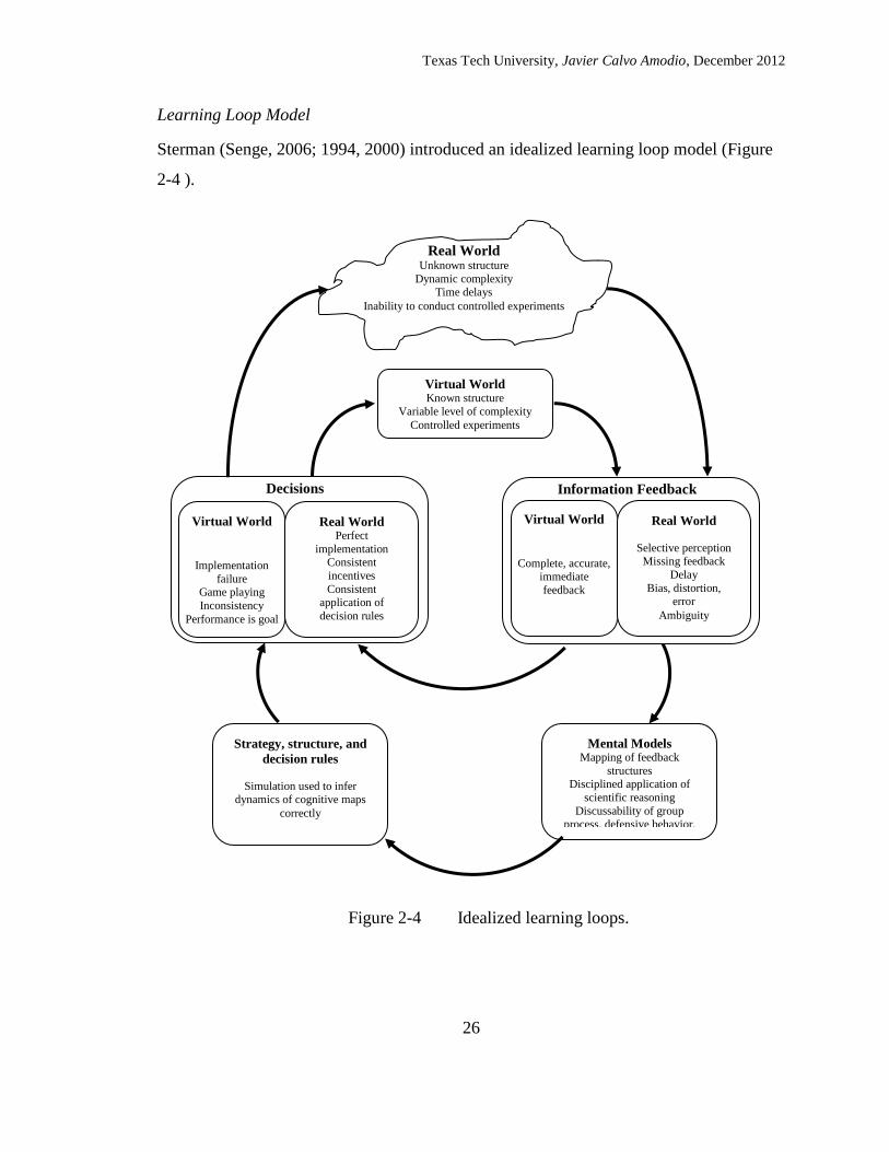
Texas Tech University, Javier Calvo Amodio, December 2012
26
Learning Loop Model
Sterman (Senge, 2006; 1994, 2000) introduced an idealized learning loop model (Figure
2-4 ).
Real World Unknown structure
Dynamic complexity Time delays
Inability to conduct controlled experiments
Virtual World Known structure
Variable level of complexity
Controlled experiments
Virtual World
Implementation
failure Game playing
Inconsistency
Performance is goal
Real World Perfect
implementation Consistent
incentives
Consistent application of
decision rules
Learning can be goal
Decisions
Virtual World
Complete, accurate,
immediate
feedback
Real World
Selective perception Missing feedback
Delay
Bias, distortion, error
Ambiguity
Information Feedback
Strategy, structure, and
decision rules
Simulation used to infer dynamics of cognitive maps
correctly
Mental Models Mapping of feedback
structures Disciplined application of
scientific reasoning
Discussability of group process, defensive behavior.
Figure 2-4 Idealized learning loops.

Texas Tech University, Javier Calvo Amodio, December 2012
27
The validity of the model Sterman introduces is that it provides a good justification for
the use of simulation models as learning tools. By simplifying reality and putting it into a
virtual world, it is possible to perform experiments within it. Policies and approaches can
be challenged without having to wait for feedback from reality, which can be expensive.
Learning Curves and System dynamics
Carrillo and Gaimon (2000), and Morrison (2008) mention that productivity in early
stages suffers even if the new process is supposed to improve productivity, and that it is
strictly related to the learning curve process. That process is also congruent with the
system dynamics principle which states that when there is an intervention on a system it
can get worse before it gets better (Sterman, 2000). Morrison (2008) also states that
cumulative production is a reflection of knowledge of the process, and that according “to
learning curve theory, the accumulation of experience increases productivity, or
alternatively reduces costs” (p. 1184). Thus identifying characteristics that are shared
with system dynamics simulation models can bring better light to the study of learning
curves. Morrison proposed the following model shown in Figure 2-5 (Morrison, 2008, p.
1185) of learning under constraints:
Figure 2-5 A model of learning by doing under constraints.
Extracted from

Texas Tech University, Javier Calvo Amodio, December 2012
28
The model stresses that the learning process is enhanced by the amount of time spent
with a new skill, which in turn increases the cumulative experience. Morrison posits that
forgetting is an intrinsic part of learning, but that enough time spent with a new skill will
offset the effects of forgetting.
Systems Thinking
Formalized systems science theory, and applied methodologies date back to the middle of
the 1900’s with the strong contributions by Ludwig von Bertalanffy’s general system
theory, Jay Forrester’s system dynamics, Russell Ackoff’s , Churchman’s and Maturana
and Varela’s autopoiesis.
The Engineering Management practice is teleologically oriented. That means that the
focus on the development of theories and their application is goal-seeking or purposeful.
Systems thinking is also teleologically oriented. Engineering management and systems
thinking are oriented to provide solutions for systems that can display choice of means
and/or ends.
[The systems age] is interested in purely mechanical systems only insofar as they
can be used as instruments of purposeful systems. Furthermore, the Systems Age
is most concerned with purposeful systems, some of whose parts are purposeful;
these are called social groups. The most important class of social groups is the
one containing systems whose parts perform different functions, that have a
division of functional labor; these are called organizations. Systems-Age man is
most interested in groups and organizations that are themselves parts of larger
purposeful systems. All the groups and organizations, including institutions, that
are part of society can be conceptualized as such three-level purposeful systems.
There are three ways in which such systems can be studied. We can try to
increase the effectiveness with which they serve their own purposes, the self-
control problem; the effectiveness with which they serve the purposes of their
parts, the humanization problem; and the effectiveness with which they serve the
purposes of the systems of which they are a part, the environmentalization
problem. These are the three strongly interdependent organizing problems of the
Systems Age (Ackoff, 1973, p. 666).
When healthcare managers embark on the implementation of a EHR, or a new billing
procedure –large purposeful systems, change management is a key element of such
purposeful system.

Texas Tech University, Javier Calvo Amodio, December 2012
29
Critical Systems Thinking
Critical systems thinking embraces five major commitments by seeking to demonstrate
critical awareness, showing social awareness, dedication to achieve human emancipation,
commitment to the development of complementary and informed development of
systems thinking methodologies at the theoretical level, and commitment to the
complementary and informed use and application of methodologies (Flood, 2010, p. 279;
Jackson, 1991, pp. 184-187).
System dynamics
System dynamics creates diagrammatic and mathematical models of feedback
processes of a system of interest. Models represent levels of resources that vary
according to rates at which resources are converted between these variables.
Delays in conversion and resulting side-effects are included in models so that
they capture in full the complexity of dynamic behaviour. Model simulation
then facilitates learning about dynamic behaviour and predicts results of various
tactics and strategies when applied to the system of interest (Flood, 2010, p.
273).
System dynamics was developed by Jay W. Forrester to model feedback loops in systems
where non-linear time dependent interactions are present. System dynamics presents a
powerful approach to modeling complex systems in accordance to what their internal
structure and interactions actually are, and not in accordance to what statistics and/or
mathematical models suggest alone. Feedback is present in non-linear systems where its
components sustain complex interactions and that emergent properties arise from such
interactions. With the use of level and rate variables, it is possible to model the
interactions and feedback loops between system components. Dynamic modeling can
help identify lack of understanding of a process or system, and to identify what are the
most important variables in a process or system (Hannon & Ruth, 2001, p. 10).
Senge (2006) advocated for the use of systems thinking as the quintessential tool to
enhance the efficacy of managerial endeavors. As Forrester’s disciple, Senge’s approach
is focused on the use of system dynamics, and causal loop models.

Texas Tech University, Javier Calvo Amodio, December 2012
30
The foundation blocks, or the common structures that describe all systems are the level
and rate equations (J.W. Forrester, 1961, 1968; 1971). Level equations result from
integrations of flows proceeding from rate inflow equations minus the integration of rate
outflows equations over time (see Equation 2-4). In its simplest form, a rate equation
depends on the state of the level variable. A rate equation regulates, depending on the
state of the level variable the flow rate (see Equations 2-3 and 2-4).
There are two graphical tools to represent the relationships expressed in Equations 2-3
and 2-4: Causal Loop Diagrams, and Level and Rate diagrams. A causal loop diagram is
a graphical representation of the interactions between the level and rate variables in the
system. In Figure 2-6 we can see the graphical representation of Equations 2-4 and 2-5.
The state of the level is determined by the inflow and outflow rates. The arrows
connecting the variables indicate the nature of the relationship (feedback) between them.
A positive feedback means that the rate change will be in the same direction as the
change observed in the level. A negative feedback means that the rate change will be in
the opposite direction of the change observed in the level. For instance, if the state of the
level increases, the inflow rate will decrease.
Inflow Rate. Level.
+
-
Outflow
Rate.
+
-
𝐿𝑒𝑣𝑒𝑙𝑡 ∫ 𝐼𝑛𝑓𝑙𝑜𝑤 𝑅𝑎𝑡𝑒 ∫ 𝑂𝑢𝑡𝑓𝑙𝑜𝑤 𝑅𝑎𝑡𝑒𝑛
𝑡=
𝑛
𝑡= Equation 2-3
𝑅𝑎𝑡𝑒𝑡
𝑑𝐿𝑒𝑣𝑒𝑙
𝑑𝑡 𝐼𝑛𝑓𝑙𝑜𝑤 𝑅𝑎𝑡𝑒𝑡 𝑂𝑢𝑡𝑓𝑙𝑜𝑤 𝑅𝑎𝑡𝑒𝑡 Equation 2-4
Figure 2-6 Causal Loop Diagram

Texas Tech University, Javier Calvo Amodio, December 2012
31
Figure 2-7 shows a Level and Rate diagram where the rate of flow and stock of goods,
materials, money, information, etc. is represented by valves and stock components. The
valves (Inflow and Outflow Rates) are controlled by the feedback received from the stock
variable (Level).
Figure 2-7 Rate and Level Diagram
A system dynamics model is constructed using, according to Forrester (1971; 1961,
1968) from the use of mental, written, and numerical databases (see Figure 2-8).
Different components of the model are extracted from these databases allowing the model
to replicate the real system characteristics accurately.
LevelInflow Rate
-
Outflow Rate
+
Policies, expectations and
structure,
Cause-to-effect direction
between variables
Concepts and abstractions,
Characteristics of learning
abilities, training sessions, etc.
Mental Data Base
Observation Experience
Written
Data Base
Numerical
Data Base
Figure 2-8 Mental Data Base and Decreasing Content of Written and Numerical
Data Bases

Texas Tech University, Javier Calvo Amodio, December 2012
32
Barlas (1996) presents a guideline on generalized steps employed to develop a system
dynamics model:
1. Problem identification
2. Model conceptualization (construction of a conceptual model)
3. Model formulation (construction of a formal model)
4. Model analysis and validation
5. Policy analysis and design
6. Implementation
The construction of a conceptual model is generally aided by the use of causal loop
diagrams.
Causal loop diagrams as mental models
Systems thinking authors such as Peter Checkland (1979a, 1979b, 1981, 1985, 1988,
1999, 2000; Checkland, Forbes, & Martin, 1990; Checkland & Scholes, 1990) and
Forrester (1961, 1971a, 1971b, 1980, 1987a, 1987b, 1991, 1992, 1994, 1995, 1999; J.
Forrester, Low, & Mass, 1974; J. Forrester & Senge, 1980) advocate for the use of mental
models to better understand, or learn about the system at hand. ‘‘The real value of
modeling is not to anticipate and react to problems in the environment, but to eliminate
the problems by changing the underlying structure of the system’’ (Sterman, 2000, pp.
655-656). Causal loop diagrams help the practitioner to uncover the underlying structure
of the system.
Efficiency, efficacy, and effectiveness of a model
When creating any model, the purpose, objectives, and benefits expected—or ends—and
the resources available – or means—must be clearly stated. Proper allocation of means
and ends can be balanced through their efficient, efficacious, and effective use within a
model. Efficiency refers to the ratio between resources used and their product (or what

Texas Tech University, Javier Calvo Amodio, December 2012
33
the outcome is). A system is efficient if the value of the outcome or the benefit is
perceived to be higher than the value of the resources employed to produce/generate it.
An efficient model should minimize efforts while maximizing the value of outcomes.
Unfortunately when special attention is paid to the means to achieve the ends a paradox
arises. This contradiction takes place because as more resources are invested to increase
the value of the benefits, those resources become more costly, making it impossible to
reach a superior model, leading to a compromise in end quality so that the feasibility of a
model is maintained ( see Figure 2-9)
∑
∑
Efficacy refers to the ability a system has to perform as and/or do what it is designed to
do. That is, the ends are what matters, regardless of the means employed. It is then, as
Figure 2-9 Ratio relationship between Resources and Benefits to achieve efficiency Resources allocated
1
0 →
Efficiency
Equation 2-3 Efficiency in model
development

Texas Tech University, Javier Calvo Amodio, December 2012
34
presented in the previous section, that achieving efficacy in a model results in a paradox,
but nonetheless is a highly desired characteristic.
Effectiveness refers to the alignment of what the system actually does and what the
system is supposed to do. That is, it questions the adequateness of the outcome produced
by the system. A system may be efficient and/or efficacious within its own design but
still fail to perform as desired, not effective1. Hence, a model is only effective if its
performance –regardless of its complexity—is aligned with what it is expected to do.
Thus, efficiency, efficacy and effectiveness, can be used to validate a model.
Procedure depends on the purpose, so the procedure presented here is valid within that
premise.
Model Validity in a System dynamics Model
C.I. Lewis (1924), states that knowledge is probable only if our experiences and/or
interpretations of the object (what we are studying, a model for instance) and the a priori
(knowledge of the real world) –through our senses are in accordance to each other. Also
that empirical truth is possible through conceptual interpretation of the given, hence we
can have an empirical object, an imaginary construct of a reality extrapolated from our
own past experiences – an a priori. Hence, a model is a valid construct to depict a
system, a selected set of parts, interactions, and characteristics of a particular given.
Validity means “adequacy with respect to a purpose” (Barlas, 1996, p. 188). Thus, if a
model is efficient, efficacious, and effective, it is valid. However, the process of model
validation has to use semi-formal and subjective components (Barlas, 1996, pp. 183,
184). For instance, a white-box model –a system dynamics model, is built to
reproduce/predict the real world behavior, and to explain how the behavior germinates.
1 It is important to note that defining efficiency and efficacy carefully is important to approach the expected
behavior of the model.

Texas Tech University, Javier Calvo Amodio, December 2012
35
Ideally, the model should also suggest ways of changing the existing behavior (Barlas,
1996, p. 186).
System dynamic models are built to assess the effectiveness of alternative policies or
design strategies on improving the behavior of a given system. Therefore, “a valid model
[is] one of many possible ways of describing a real situation” (Barlas, 1996, p. 187).
Barlas (1996) presents a summary of activities that can be used to validate a system
dynamics model based on a literature review (see Figure 2-10).
The structure confirmation test, requires comparison of the form of the equations of the
model against the real system (J. Forrester & Senge, 1980) as part of the mental database
and correspondence with the numerical database (as presented in Figure 2-8). The
comparison to the written database is called a theoretical structure test. It is conducted by
comparing the model equations with knowledge found in the literature (Barlas, 1996, p.
190).
The information used to validate the structure of the model is qualitative in nature, a
process similar to the validation of computer models in that the structures and data flows
are compared to the real world. It is important to test individual expressions to extreme
conditions and see if they still behave in a manner that could be expected in the real
world. Structural tests should be applied to the whole model and to subsections of the
model through simulation of normal and extreme conditions. With these tests, the
sensitivity of the model is to be uncovered, changes can be made, or at least unreliable
operation conditions are uncovered.

Texas Tech University, Javier Calvo Amodio, December 2012
36
Figure 2-10 Overall nature and selected tests of formal model validation

Texas Tech University, Javier Calvo Amodio, December 2012
37
System dynamics in healthcare
Homer (J. Homer & Oliva, 2001)has advocated the use of system dynamics in healthcare
environment. In particular, Homer advocated the use of System dynamics as a tool to
identify and control chronic illness underlying structures (J. B. Homer & Hirsch, 2006).
Electronic Health Records (EHR)
The Electronic Health Record (EHR) is a longitudinal electronic record of patient health
information generated by one or more encounters in any care delivery setting. Included
in this information are patient demographics, progress notes, problems, medications, vital
signs, past medical history, immunizations, laboratory data, and radiology reports. The
EHR automates and streamlines the clinician's workflow. The EHR has the ability to
generate a complete record of a clinical patient encounter - as well as supporting other
care-related activities directly or indirectly via interface - including evidence-based
decision support, quality management, and outcomes reporting
(http://www.himss.org/ASP/topics_ehr.asp).
Miller and Sim (2004) present some barriers to the implementation of an electronic health
records system. Their research showed that high initial financial costs, slow and
uncertain financial payoffs, and high initial physician time costs are barriers to
implementing electronic health records. They add that difficulties with technology,
complementary changes and support, electronic data exchange, financial incentives, and
physicians’ attitudes are also underlying barriers.
Yoon-Flannery et al (2008) identified six themes that are important to an EHR
implementation: 1. communication, 2. system migration, 3. technical equipment, support
and training, 4. patient privacy, 5. efficiency, and 6. financial considerations.
Communication must be fluid between executives, practitioners, and vendors; with clear
leadership, and communication of performance expectations. System migration must be
smooth and avoid loops or gaps in information access, as these could be critical in
treating patients. Technical equipment, support, and training are viewed as a pivotal
element of an EHR implementation. Support is vital to help practitioners, for instance,
equipment must be available at all times; if that is not possible, contingency plans must
be in place to minimize potential problems. Patient privacy is considered to be a priority

Texas Tech University, Javier Calvo Amodio, December 2012
38
and there is a belief that it can help increase patient privacy; however there is a concern
that the electronic health records system may be vulnerable to unauthorized access to
patients data. Since the implementation of the electronic health records requires some
changes to be made to the workflow and processes, there is a concern of whether the
efficiency will be affected negatively by its implementation. Finally, expenses to install
and operate the system, and how the new system will affect the personal incomes must be
clarified to the users.
Zandieh et al (2008) report that communication with patients and access to more
complete data to make more knowledgeable diagnoses, is an advantage of an electronic
health records system. They also report that a more streamlined process can be a result of
an EHR implementation after a period of 4-6 months of inefficiency (specifying 2-3
weeks of disastrous inefficiency).
Adler (2007) suggests that successful electronic health records system implementations
are influenced by three dimensions: teams, tactics and technology. He posits that teams
may suffer in large or small organizations because it is hard to form synergy and in small
organizations they may suffer due to lack of experience. Regarding tactics, he says that
they affect both large and small organizations due to planning, workflow redesign, data
entry, interfaces, training, going live, and big bang versus phased type implementations.
Technology also has an impact if networking, speed of data transfer, IT support, and
maintenance are not properly catered for.
McGowan, Cusack, and Poon (2008) state that the system selection in an electronic
health records system implementation should be driven by organizational issues and the
desired outcomes. These desired outcomes should be incorporated into a formative
evaluation plan. They define formative evaluation as “an iterative assessment of a
project’s viability through meeting defined benchmarks, can mean the difference between

Texas Tech University, Javier Calvo Amodio, December 2012
39
success and failure in EHR implementation” (p. 297). This effort aligns with lean
thinking’s continuous improvement approach.
Lo et al (2007) conducted a time and motion study to evaluate whether an electronic
health records system would add time to practitioners’ activities compared to traditional
paper forms. They concluded that there is a non-significant increase in the overall time
practitioners spend given enough time (they mention 9 months of learning). They also
found that there is no need to develop particular versions of the software for specialists
(cardiologist, ophthalmologists, etc.) since a generalized version will perform as well.
Pizziferri et al (2005) conducted a time motion and study in an oncologist setting and
concluded that an EHR system will not take more time than the traditional paper records
keeping method.
Terry et al (2008) state that finding the time to train, practice and learn the EHR is the
biggest problem physicians identified. The authors also mention that the level of
computer literacy has an effect on how fast of the user will transition to the new system.
Yoon-Flannery et al (2008) report that improved access and completeness of patient
records is an advantage of EHR use. Another advantage to the use of EHR is the
capability to record more data that can lead to better reports and population analyses, all
of which will help with compliance with regulations and can help increase quality of
healthcare.
Complementarist Approach
Midgley (1990, 1997) introduces an evolution of total systems intervention, called
creative methodology design. The premise is to identify the problem context, revise
suitable methodologies, and select all, or parts of the methodology that fit the problem
context. Many methodologies are comprised of parts that may each be suitable separately

Texas Tech University, Javier Calvo Amodio, December 2012
40
to different problem contexts. However, it is possible to use commensurable2
methodology parts to create an ad hoc methodology that fits the problem context of
interest. This approach will be employed in the development of the theoretical model.
The approach will also serve as the foundation for the remainder of this work.
Theoretical Model
In this chapter, relevant theoretical foundations to build the proposed theoretical model
have been presented. It is the intention of this section to provide the theoretical
foundations to the methodologies to be presented in chapter III, and used in chapters IV,
V, VI, and VII. Systems archetypes provide generalized structures that describe common
behaviors over time on a wide array of contexts and settings. Levy’s adaptation function
(1965) introduces a goal-seeking behavior to the learning curve body of knowledge.
Equation 2-4 is adapted from Equation 2-3 to include errors per day as the variable of
interest.
[ ] Equation 2-4
where Q(t) = percentage of errors per day at time t
P = desired rate of output expressed in errors per day
a = initial efficiency of the process expressed in percentage of
errors
µ = process rate of adaptation expressed in percentage of errors
t = cumulative time
Equation 2-5 generates an exponential decay goal-seeking behavior until the initial
percentage of errors per day reaches the desired percentage of errors per day. Figure 2-11
presents the expected behavior over time as expressed by Equation 2-6.
2 Commensurble refers the compatibility that a methodology has with a problem context. In the context
above: A section of a methodology may be commensurable to a different problem context than the parent
methodology; and different commensurable parts of methodologies can be used to create a new ad hoc
methodology. See Midgley (1990, 1997) and Wilby (1997) for details.

Texas Tech University, Javier Calvo Amodio, December 2012
41
The initial approach to link the adaptation function behavior over time to a system
archetype is to look at the ‘balancing loop’ structure and its corresponding behavior over
time (see Figure 2-12). The action causes the current state to move towards the desired
state.
Figure 2-12 ‘Balancing Loop’ Causal Loop Diagram and Behavior Over Time
Graph
Desired State Gap
ActionCurrent State
+-
+
+
Current State
Desired State Gap
Qt=state of the system at time t
Q0=Initial
State
P = Desired
state
Original State
Training
Period t0
Transition Phase tf Successful Implementation
t
% e
rro
rs
per
day
Figure 2-11 Levy's Adaptation Function seen as behavior over time graph

Texas Tech University, Javier Calvo Amodio, December 2012
42
At first glance, the ‘balancing loop’ appears to be a good fit to the behavior over time
described in Figure 2-11. However, in reality a transition-phase will not occur without
glitches or inconsistencies. For instance, the balancing loop ignores the effects of factors
like forgetting, employee absenteeism, different levels of experience, varying learning
abilities, pressure to manage resources, and pressure to complete the project on time.
The ‘drifting goals’ archetype can model the pressure generated by any deviations from
the original plan, which may result in changes on deadlines, or target state. Figure 2-13
presents the ‘drifting goals’ archetype using causal loops.
Figure 2-13 ‘Drifting Goals’ Causal Loop and Behavior Over Time Graph
Notice how the lack of convergence from the current state concerning the desired state
generates pressure to adjust either the target percentage of errors per day or the deadline.
Desired State
Gap
Action
Current State
+
-
+
+Pressure to
adjust desire
-
+
% errors
t
Current State
Desired
State
Gap
Pressure to Adjust

Texas Tech University, Javier Calvo Amodio, December 2012
43
The current state may differ from the desired state due to errors in planning that cause
unintended consequences. The ‘fixes that fail’ archetype would be the option. Figure 2-
14 presents the ‘fixes that fail’ archetype in causal loop format.
Figure 2-14 ‘Fixes that Fail’ Causal Loop and Behavior Over Time Graphs
Desired State
Gap
Action
Current State
+
-
+
+
UnintendedConsequences
+
-
Current State
Desired
State
Gap
% e
rro
rs
t
Current State
Desired
State
Gap
%
erro
rs
t
Current State
Desired
% of errors
Gap
% e
rro
rs
t
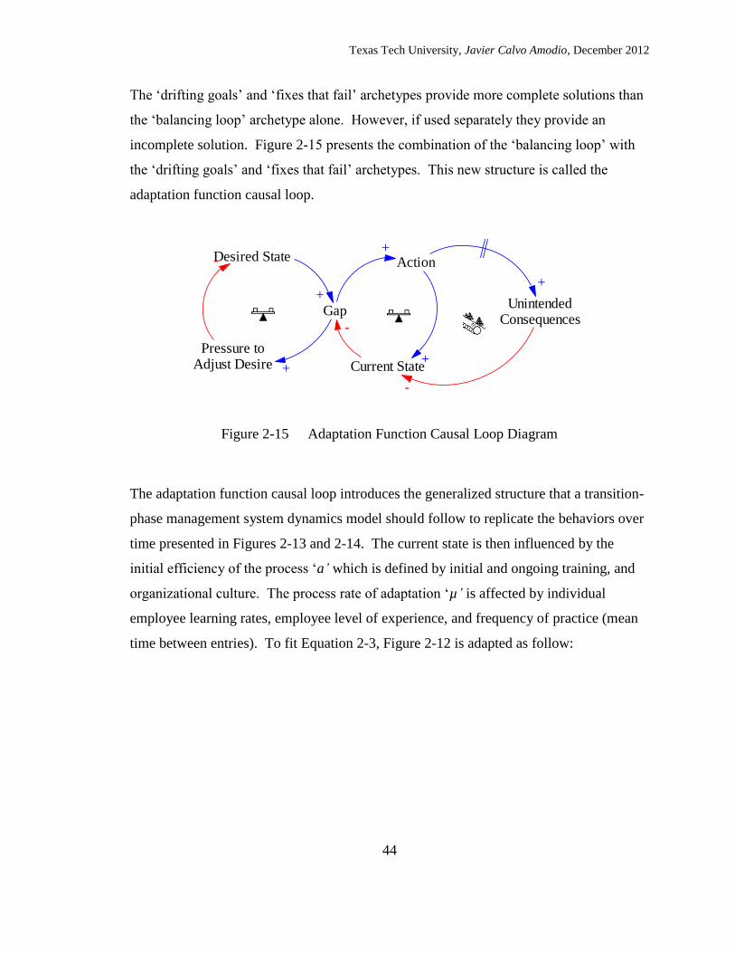
Texas Tech University, Javier Calvo Amodio, December 2012
44
The ‘drifting goals’ and ‘fixes that fail’ archetypes provide more complete solutions than
the ‘balancing loop’ archetype alone. However, if used separately they provide an
incomplete solution. Figure 2-15 presents the combination of the ‘balancing loop’ with
the ‘drifting goals’ and ‘fixes that fail’ archetypes. This new structure is called the
adaptation function causal loop.
The adaptation function causal loop introduces the generalized structure that a transition-
phase management system dynamics model should follow to replicate the behaviors over
time presented in Figures 2-13 and 2-14. The current state is then influenced by the
initial efficiency of the process ‘a’ which is defined by initial and ongoing training, and
organizational culture. The process rate of adaptation ‘µ’ is affected by individual
employee learning rates, employee level of experience, and frequency of practice (mean
time between entries). To fit Equation 2-3, Figure 2-12 is adapted as follow:
Desired State
Gap
Action
Current State
+
-
+
+
UnintendedConsequences
+
-
Pressure toAdjust Desire
-
+
Figure 2-15 Adaptation Function Causal Loop Diagram
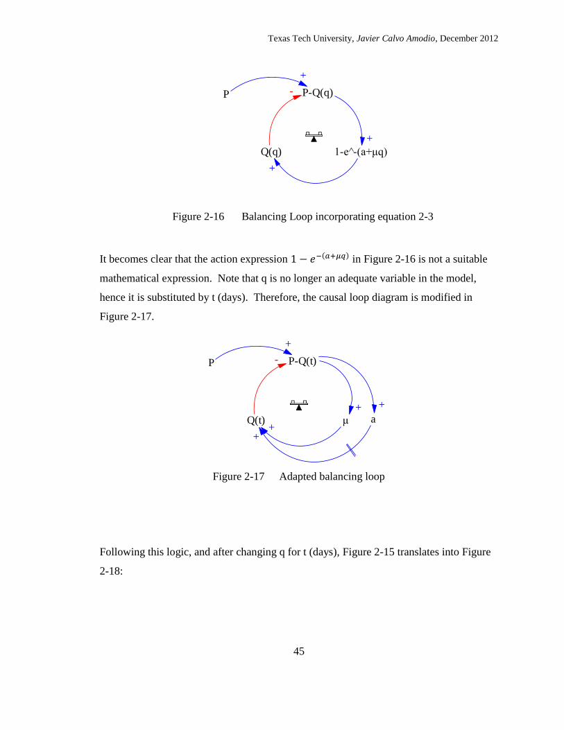
Texas Tech University, Javier Calvo Amodio, December 2012
45
It becomes clear that the action expression in Figure 2-16 is not a suitable
mathematical expression. Note that q is no longer an adequate variable in the model,
hence it is substituted by t (days). Therefore, the causal loop diagram is modified in
Figure 2-17.
Following this logic, and after changing q for t (days), Figure 2-15 translates into Figure
2-18:
P P-Q(q)
1-e -(a+μq)Q(q)
+
-
+
+
Figure 2-16 Balancing Loop incorporating equation 2-3
Figure 2-17 Adapted balancing loop
P P-Q(t)
μQ(t)
+
-
+
+a
+
+
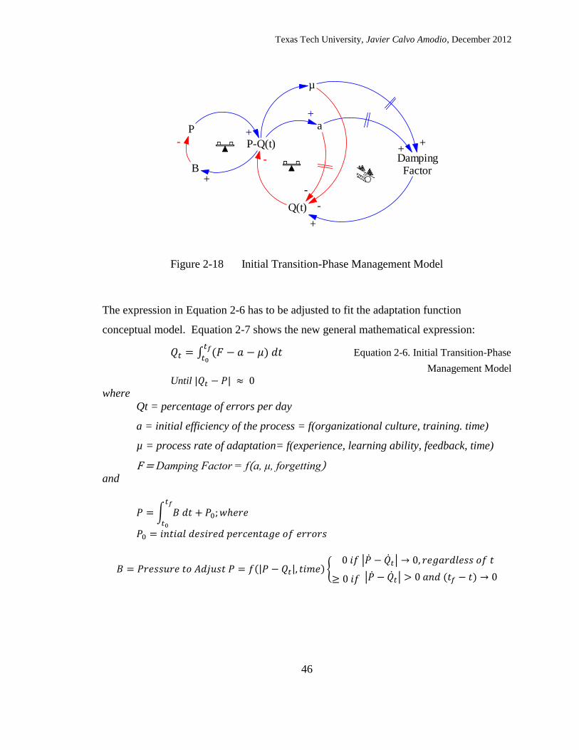
Texas Tech University, Javier Calvo Amodio, December 2012
46
The expression in Equation 2-6 has to be adjusted to fit the adaptation function
conceptual model. Equation 2-7 shows the new general mathematical expression:
∫
Equation 2-6. Initial Transition-Phase
Management Model Until
where
Qt = percentage of errors per day
a = initial efficiency of the process = f(organizational culture, training. time)
µ = process rate of adaptation= f(experience, learning ability, feedback, time)
and
∫
{ | |
| |
Figure 2-18 Initial Transition-Phase Management Model
P
P-Q(t)
a
Q(t)
+
-
+
-
DampingFactor
+
+
B
-
µ
+
-
+
Desired Percentageof Errors per Day

Texas Tech University, Javier Calvo Amodio, December 2012
47
P is a variable that determines the desired percentage of errors per day set at an expected
completion time or tf, therefore:
Equation 2-5 Desired State
Pressure to Adjust P (B) is a dimensionless function based on the relationship between
time remaining to complete the project (tf−tobs), a time determined by manager’s policy to
start evaluating the progress (Panic Time) and the difference between the percentage of
errors per day and the desired state at time t (Qt−P).
Equation 2-6 Pressure to Adjust
Where
The model is capable of providing the following alternatives as objective functions
(Figure 2-19).
Figure 2-19 Objective Function for Transition Phase Management Model
Quality
min P-Qt
Time
min tf-t0
Cost
min a + µ

Texas Tech University, Javier Calvo Amodio, December 2012
48
Balance between vertices in the triangle means that in order to optimize one apex, one of
the two remaining vertices cannot be optimized.
It is hypothesized then that the model is capable of helping healthcare managers to:
1. Maximize the quality of a new process implementation through the balance of
resource cost allocation and time to complete the project.
2. Minimize the use of resources through the balance of time to complete the project
and quality.
3. Optimize the time required to complete the project through balancing quality and
use of resources.
Section 8.1 presents the conclusions on how to Figure 2-19 relates to the work presented
in this dissertation.

Texas Tech University, Javier Calvo Amodio, December 2012
49
CHAPTER III
3. METHODOLOGY
Introduction
The purpose of this chapter is to provide an outline of the research methodology used in
this research. The chapter provides details on how the research methodology will be
divided into three tasks and two experiments. The chapter explains how the tasks and
experiments are allocated into one conference paper and three different peer reviewed
journal research papers.
Rationale
The rationale for this research is to increase the understanding of the dynamic
interactions that occur during transition-phases in healthcare projects.
Research Design
Barlas (1996, p. 185) provides a list of six major steps typically followed in the
construction of a system dynamics model.
1. Problem identification
2. Model conceptualization (construction of a conceptual model)
3. Model formulation (construction of a formal model)
4. Model analysis and validation
5. Policy analysis and design
6. Implementation
This dissertation will focus on steps one through four as specified in Table 3-1 as steps 5
and 6 are left for the healthcare managers that will use it.

Texas Tech University, Javier Calvo Amodio, December 2012
50
Table 3-1 Research Design Steps
Step Research Scope Design Overview
1. Problem identification Chapter 1 Described through problem statement,
research questions, and hypotheses.
2. Model conceptualization
(construction of a
conceptual model)
Theoretical Model
presented in
section 2-3.
Developed after adaptation function,
and system dynamics theories.
The model will be included in a
conference paper.
3. Model formulation
(construction of a formal
model)
Task 1
The generalized model formulation
after the theoretical model in section
2-3 will start with a pilot study
presented in a conference paper.
It will develop sub-structures in paper
one and will be validated with real
world data in papers two and three.
4. Model analysis and
validation
Tasks 2 and 3
Experiments 1 and
2.
For paper 1, a double loop learning
process will be followed.
For papers 2 and 3, the process
presented in Figure 2-10 will be
employed.
5. Policy analysis and
design
Outside the scope
of this
dissertation.
Future work.
6. Implementation Outside the scope
of this
dissertation.
Future work.
Texas Tech University, Javier Calvo Amodio, December 2012
51
This dissertation follows a four-paper format. The theoretical model presented in section
2-3 will serve as the starting dynamic structure from which tasks 1, 2 and 3 are derived.
The recognition of the problem is stated in section 1-2, and it reads:
Combining industrial engineering and engineering management tools to improve
a particular problem situation in the healthcare industry has proven successful.
The use of industrial engineering and engineering management tools (scientific
management approach) to improve operation conditions and maximize revenue
has been gaining popularity in the health care environment. Examples range
from the implementation of the TQM model, to the incorporation of Lean
thinking and Six Sigma methodologies. However, research of transition-phases
in a healthcare environment, using a holistic scientific management approach, has
received little attention. The estimation of time and resources required to
conduct a transition-phase, usually employs “rule of thumb” approaches based on
simple calculations– rather than a holistic scientific management method. A
systemic approach to manage transition-phases will bring a dynamic approach to
manage transition-phases during planning and implementation stages.
Task 1 will conclude as a conference paper presented in chapter 4. Tasks 2 and 3 will
result in a peer reviewed journal paper and will be included in chapter 5. Experiments 1
and 2 will result in two peer reviewed journal papers and will be presented in chapter 6
and 7 respectively. Chapter 7 will present general findings applicable to the dissertation,
and chapter 8 will introduce conclusions and future work analysis derived from chapter 7.
Type of Research
The research type followed in this research follows the standard approach to system
dynamics model development as presented by Barlas (1996)and Sterman (2000) but can
be best exemplified by a matrix presented by Dr. Simon Hsiang3 in his design of
experiments class as he proposed the following model for model validation:
3 From IE5342 Design of Experiments class, Fall 2011.

Texas Tech University, Javier Calvo Amodio, December 2012
52
Table 3-2 Model Validation Matrix
Characteristic Order
of first
run
Input Model Output Verification
Stage
System Identification 1 Known Unknown Known
Simulation 2 Known Known Unknown
Control 3 Unknown Known Known
The process is iterative and non-linear, as with any simulation model. For illustration
purposes, the first iteration is described. The first step is to develop the dynamic
hypotheses (identify expected behaviors over time) through the system identification.
The first attempt is presented in section 2-3 as the theoretical model. The second step
requires the translation of the theoretical model into a simulation model in a pilot study
form. The pilot study will then lead to step three, where the identification of inputs will
aid the data collection for experiments 1 and 2. After that point, steps one through three
will alternate until a validated structure, within the parameters defined in the testable
hypothesis, are rejected, or fail to be rejected.
Research Focus
The creative methodology design approach to total systems intervention is based –as
specified in section 2-3, on Levy’s adaptation function. The adaptation function is
interpreted as behavior over time under a system dynamics framework. The focus in this
dissertation is to develop a transition-phase management system dynamics model that is
capable of replicating real world behavior over time in a healthcare transition-phases.
Research Hypotheses Restated
In chapter I, three tasks and two general research hypotheses were stated. Each of these
hypotheses belongs to one experiment. This dissertation follows the three papers format,
hence tasks 2 and 3, and experiments 1 and 2 will result in research papers.

Texas Tech University, Javier Calvo Amodio, December 2012
53
Table 3-3 Outputs and Target Publications
Activity/Test Output Target Publication
Task 1 Conference Paper 2012 ASEM International
Annual Conference
Tasks 2 and 3 Peer Reviewed Journal Paper Engineering Management
Journal
General Research
Hypothesis 1
Peer Reviewed Journal Paper IIE Transactions in healthcare,
or a healthcare management
journal
General Research
Hypothesis 2
Peer Reviewed Journal Paper Engineering Management
Journal, or System Dynamics
Review
Tasks
Task 1: Develop a pilot study to translate the initial Transition-Phase
Management Model (see Figure 1-2 and Equation 1-1) into a stock and flow
diagram (will translate into a conference paper).
Task 2: Further define the model by developing the sub-structures for a, µ,
Damping Factor and B.
Task 3: Test the model for inputs limits and validity of outputs ( tasks 2 and 3 will
translate into a peer reviewed journal paper).
Hypotheses
The model developed in tasks 1, 2, and 3 will be used as the template to run experiments
1 and 2, as presented below.

Texas Tech University, Javier Calvo Amodio, December 2012
54
General hypothesis for Experiment 1:
The transition-phase errors per day in a hospital billing process necessary as a result of an
electronic health records system implementation can be depicted with the transition-phase
management model.
d) The information available (quantitative and qualitative) to the manager at a
local healthcare center is adequate to generate the desired behavior over time.
e) The model is capable of identifying the path that the percentage of errors per
day will follow during the implementation process
f) The model is able to identify when and if dynamic equilibrium is reached
General hypothesis for Experiment 2:
The changes to a hospital’s clerical processes induced by the implementation of an
electronic health records system can be depicted with the transition-phase management
model.
d) The information available (quantitative and qualitative) to the manager at
Community Health Center of Lubbock is adequate to generate the desired
behavior over time.
e) The model is capable of identifying the path that the percentage of errors per
day will follow during the implementation process
f) The model is able to identify when and if dynamic equilibrium is reached
a) the expected effects that the feedback structures have on errors per day.
Tasks 1, 2 and 3, and experiments 1 and 2 serve to generate a model that will facilitate
the double loop learning process in an organization (see Figure 2-4) by reducing the time
to develop a virtual world and providing a reliable structure to analyze the real world.
According to these general hypotheses and Table 3-3, the general hypotheses that deal
with model validity are presented in Table 3-4. Table 3.5 presents specific testable
hypotheses for experiments 1 and 2.

Texas Tech University, Javier Calvo Amodio, December 2012
55
Table 3-4 General Testable Hypotheses Matrix
Tests for Hypothesis Hypothesis Proposed Test
Task 3
1
H0: The µ substructures have no effect on
the percentage of errors per day for all t:
1. Extreme
values test using
built in
sensitivity
analysis in
Vensim using
uniform and
triangular
distributions
2. Data sub-set
Variance Plot
2
H0: The a substructures have no effect on
the percentage of errors per day for all t:
3
H0: The F substructures have no effect on
the percentage of errors per day for all t:
4
H0: The B substructures have no effect on
the percentage of errors per day for all t:
Experiments
1 and 2
5
H0: Percentage of errors per day (Qt) model
generated data replicates the behavior of the
real world percentage of errors per day (QRt)
for short, mid and long-term projects:
1. Paired Two
Sample for
Means R2
2. Histogram of
Differences QR -
Q
3. Graphical
comparison
between Q and
QR
6
H0: Percentage of errors per day (Qt) model
generated data predicts the path of the real
world percentage of errors per day (QRt) for
short, mid and long-term projects:
tH
H
ta
tttt f
allfor 0:
0 :2100
taH
aaaaH
ta
tttt f
allfor 0:
0 :2100
tFH
FFFFH
ta
tttt f
allfor 0:
0 :2100
tBH
BBBBH
ta
tttt f
allfor 0:
0 :2100
Texas Tech University, Javier Calvo Amodio, December 2012
56
Collection and Treatment of Data
Two sources of data were employed: a local healthcare clinic’s clerical processes and a
local healthcare center’s billing department. The data used is historical in nature, aiding
in the validation process for the models.
Data Collection
Quantitative Data
Per Internal Review Board (IRB) requirements, all quantitative data were to be retrieved
by personnel from each organization, and any identifiers were to be coded, so that no
individuals’ data could be traced back (see appendix A for IRB proposal). System
dynamics model-building strategies suggest starting with simple structures and increasing
complexity gradually until the desired levels of accuracy are reached. In the case of this
research two levels of resolution were deemed sufficient.
Qualitative Data
System dynamics models allow the use of qualitative data when quantitative data is not
available, or when it is necessary to define some behavior over time parameters.
Collection of qualitative data followed the same process described in section 3.4.1.1, with
the distinction that the data was recorded directly from informal interviews with the
managers.
Simulation
Model calibration followed Table 3-3. Once the parameters replicated the expected
behavior over time after goal programming-style calibration, a sensitivity analysis of all
variables was conducted through the built in sensitivity function in the simulation
package (Vensim Professional) and are presented in chapter 5.

Texas Tech University, Javier Calvo Amodio, December 2012
57
Case Study
A pilot study was developed –and presented in chapter 4 using the theoretical model
presented in section 2-3 to complete task 1. Parameters were adjusted based on mental
and written databases (see Figure 2-8) following a goal programming approach. The
pilot study’s objective is to observe if the structure replicates the expected behaviors over
time of the initial transition-phase management model structure. Tasks 2, and 3 propose
specific structures for efficiency of the process, process rate of adaptation, and Damping
Factors substructures introduced in task 1. The objective is to produce a model that can
be applied within a healthcare context when managing changes brought by electronic
health records system implementation and changes in billing procedures are of interest.
Treatment of Data
The data obtained was utilized “as is” to compare it versus the model. Some outlier data
points were removed due to special circumstances such as capture errors or data
generated under special circumstances such as holidays or weekends. The justification to
minimize as much as possible data treatment follows two points:
1. The data collected is the data managers work and make decisions with.
2. System dynamics can help detect errors in data collection if the expected
behavior over time cannot be replicated. In that case, what needs to be treated
is the data collection method, not the data.
Methodological Issues
Reliability
Reliability is the accuracy of the research, its efficacy, and effectiveness. It refers to how
well the model will yield certain expected results as long as the entity being measured
does not change. Reliability in this research is given in two steps. The first one is
achieved in experiments 1 and 2 through the validation of their substructures in
hypotheses. The second one is obtained through the cross-validation of their

Texas Tech University, Javier Calvo Amodio, December 2012
58
substructures. In both cases, the reliability will follow the process delineated in Table 3-
2, and expanded in Table 3-5.
Validity
Model validity depends on the non-linear process of identifying the system’s structure,
performing simulation to calibrate its output (or outputs), and controlling the inputs, with
regards of level of detail and nature –qualitative, quantitative or a mix of both. Table 3-5
presents a detail depiction of the model validation process to be used in this dissertation.
Table 3-5 is based on Table 3-2.
Table 3-5 Detailed Model Validation Matrix
Characteristic
Verification
First
run
order
Input Model Output Product
Hypotheses
from Table
3-4
System
Identification 1 Known Unknown Known
Conference
Paper
Theoretical
Model Task
1
Paper 1 Tasks 2, and
3
Simulation 2 Known Known Unknown
Paper 1 Task 3
Paper 2 Hypothesis 1
Paper 3 Hypothesis 2
Control 3 Unknown Known Known Paper 1 Hypothesis 1
Paper 2 Hypothesis 2
Each validation step, followed an iterative three-step process based on Total Systems
Intervention (Flood & Jackson, 1991): A Creativity phase, and Choice Phase, and an
Implementation phase. For instance, the system identification step requires the use of
creativity to generate the structures required to duplicate the expected behavior over time.
It requires the researcher in conjunction with the managers to choose the right structure
that mimics the real world structure. The implementation of the structure is done through
the pilot study, where this initial structure is tested. The simulation step requires

Texas Tech University, Javier Calvo Amodio, December 2012
59
creativity to select the best parameters to produce the expected output(s). The control
phase requires creativity to expand the original structures and to identify what type of
information can be used to increase the model’s validity. Figure 3-1 presents the
validation structure followed.
Thus, the combination of the mental, written, and numerical databases (see Figure 2-8)
will yield the structures for efficiency of the process, process rate of adaptation and
damping factors structures and parameter estimations needed in each validation step.
Replicability
Replicability will be addressed mainly in experiment three (paper three). The objective
of paper three is to produce a generalized transition-phase management model, which
relies on replicability within a healthcare change environment.
Bias
As with any simulation model, there exists inherent bias because of the simplification of
the real world resulting from the abstraction and modeling process.
SystemIdentification
ControlSimulation
Creativity
Choice
Implementation
Creativity.
Creativity .
Implementation. Implementation .
Choice.
Choice .
Figure 3-1 Model Validation Process

Texas Tech University, Javier Calvo Amodio, December 2012
60
Representativeness
This research is representative of transition-phase projects in healthcare contexts.
Research Constraints
The main purpose of this research is to produce a generalized transition-phase
management model for healthcare contexts. For that reason, ad hoc methods to collect
data and validate data will not be developed. In addition, the expected variables
measured and outputs are bounded by the requirements that the healthcare clinic and
center selected have at the time this research is conducted.
Model Development, and Validation
This dissertation is structured to follow a four paper route. Therefore, instead of
following a more conventional approach with a chapter dedicated to data collection,
analysis and discussion and another one for conclusions, one chapter is dedicated to
present the theoretical model (based on section 2.3), one chapter addressing Hypotheses
1-4, and one chapter addressing hypotheses 5 and 6 (Table 3-4).
Validation of the model (Figure 3-5) is conducted in accordance to the schedule
presented in Table 3-6..

Texas Tech University, Javier Calvo Amodio, December 2012
61
Table 3-6 Model Validation - Chapter Relation
Characteristic
Verification
First
run
order
Input Model Output Chapter
Hypotheses
from Table
3-4
System
Identification 1 Known Unknown Known
Chapter V
Theoretical
Model Task
1
Tasks 2, and
3
Simulation 2 Known Known Unknown
Task 3
Hypothesis 1
Hypothesis 2
Control 3 Unknown Known Known Chapters VI
and VII
Hypothesis 1
Hypothesis 2
Texas Tech University, Javier Calvo Amodio, December 2012
62
CHAPTER IV
4. A PROPOSED CONCEPTUAL SYSTEM DYNAMICS MODEL FOR MANAGING
TRANSITION-PHASES IN HEALTHCARE ENVIRONMENTS
Abstract
Engineering management practice and research has gained popularity since the dawn of
the new millennium. Efforts in development and application of lean thinking and six
sigma into the healthcare industry have been steadily increasing. In addition, the
healthcare industry is faced with changes in regulations, whether small –changes in
billing procedures or large –implementation of electronic health and medical records
systems. These challenges require processes to be modified, whether on a small or large
scale, or in a superficial or deep way. Yet, little attention has been paid to the
management of these transition phases using a scientific management approach. The
purpose of the work presented in this paper is to introduce a conceptual transition phase
management model. The model is based on system dynamics principles, and borrows
concepts from change management and learning curve theories. Engineering managers
can benefit from the model in two ways: 1) the model can be employed to conduct
qualitative behavior over time analyses and 2) the model possesses the potential to be
developed as a simulation model.
Key Words. System Dynamics, Healthcare Management, Change Management,
Complementarism, Total Systems Intervention.
Introduction.
The healthcare industry is under increasing expectations to implement electronic health
records and electronic medical records systems. This pressure is placing a burden on
available human resources in healthcare institutions during implementation phases.
healthcare managers are confronted with the challenge to balance workloads, ensure

Texas Tech University, Javier Calvo Amodio, December 2012
63
transitions from old to new systems, and minimize the time it takes to implement the new
systems. In this paper, the authors present a conceptual model of a generalized transition-
phase management model for health care institutions.
The model is built using a complementarist approach to bring together Ferdinand Levy’s
adaptation function (1965) and Jay Forrester’s system dynamics. The methodology
draws on complementarism concepts introduced through Totals Systems Intervention
(TSI) by Robert Flood & Michael Jackson (1991) and Gerald Midgley (1990, 1997). The
rationale behind TSI is that to build ad hoc robust methodologies, the strengths of
individual methodologies with respect to the problem context can be combined.
Background
Frederick Winslow Taylor laid out the road map for the industrial engineering and
engineering management professions. Most industrial engineering and engineering
management methodologies were developed after Taylor published his book “The
Principles of Scientific Management” (Taylor, 1911). In his book Taylor stated that “[it]
is true that whenever intelligent and educated men find that the responsibility for making
progress in any of the mechanic arts rests with them, instead of upon the workmen who
are actually laboring at the trade, that they almost invariably start on the road which leads
to the development of a science where, in the past, has existed mere traditional or rule-of-
thumb knowledge” (Taylor, 1911, p. 52).
With the ever increasing specialization and increased requirements on knowledge
workers, Taylor’s statement re-gains importance. As the 20th century closed and the 21st
century dawned, industrial engineering and engineering management practitioners kept
developing more and more methods and methodologies to improve the "laboring trade"
as Taylor stated. Engineering Management methods once deployed have demonstrated
great levels of efficiency, efficacy, and/or effectiveness. However, as they become more
widespread in use and knowledge, the effect that they can have on a problem situation is
minimized. As a result, philosophies or toolboxes such as Lean and Six Sigma have been

Texas Tech University, Javier Calvo Amodio, December 2012
64
developed. Yet, the existing methodologies that advocate for the use of many of
industrial engineering and engineering management together lack a systemic approach
(Calvo-Amodio, Tercero, Hernandez-Luna, & Beruvides, 2011).
The approach to understanding a system’s behavior can be traced in the western world all
the way back to the Greek philosophers. Over the centuries, isolated efforts were made
by philosophers and thinkers alike. Yet, there were no strong advancements to unify the
field. The dawn of the twentieth century yielded structured efforts to develop an applied
holistic approach, known as systems thinking, for better understanding a system’s
behavior. Systems thinking as a science arose as the result of the efforts from researchers
from varied backgrounds such as biology, sociology, philosophy and cybernetics to
explain holistically the systems they studied (Jackson, 2000). Amongst the best-known
and influential authors, we find Ludwig von Bertalanffy, Charles West Churchman,
Russell Ackoff, Jay Forrester, Humberto Maturana and Francisco Varela, Stafford Beer,
and Peter Checkland.
Applied systems thinking methodologies in the management sciences started to appear as
early as the mid-1950s with the early efforts from Russell Ackoff and Jay Forrester.
Applied systems methodologies were developed to solve particular problems observed or
encountered by their authors. Each methodology was developed under assumptions that
would not necessarily be consistent or commensurable with the others. Robert L. Flood
and Michael C. Jackson from the University of Hull in the U.K. recognized this as a
problem. They developed a System of Systems Methodologies to help the user match a
particular methodology to the problem context they were interested in acting upon. They
also developed a meta-methodology called Total Systems Intervention that allows the
practitioner to combine incommensurable methodologies together. Flood and Jackson
state that problems can be classified in a grid of problem contexts that contains two
dimensions: one dimension to evaluate the relationship between the participants in the

Texas Tech University, Javier Calvo Amodio, December 2012
65
system; the second dimension to assess the complexity of the system (Flood & Jackson,
1991, p. 42). Table 4-1 shows an adaptation of the grid of problem contexts.
Notice how the applied systems thinking methodologies have been classified according to
the problem context they are best suited to be used (for more details on the grid of
problem contexts refer to Flood & Jackson, 1991, Jackson 1984, 1990, 2000). The grid
of problem contexts provides a very useful approach to identify within each problem
context, which methodology is the best suited to tackle it.
Another contribution by Flood and Jackson is a meta-methodology called Total Systems
Intervention (TSI). It allows the user to combine methodologies within or with different
problem contexts at the same time. However, there have been no attempts to provide
more detailed methodologies to combine particular tools, in a complementary way, into
more detailed approaches to modeling.
Table 4-1 Grid of Problem Contexts
Relationship Between participants
Syst
em C
om
ple
xit
y
Unitary Pluralist Coercive
Sim
ple
Systems Engineering,
Operations Research,
Statistical Quality Control,
System dynamics
General Systems Theory,
Social Systems Design,
Strategic Assumption
Surfacing and Testing
Creative
Problem
Solving,
Critical Systems
Heuristics
Com
ple
x
System dynamics, Viable
System Model, Socio-
technical Systems
Interactive Planning,
Interactive Management,
Soft Systems
Methodology,
Not Defined
Traditional industrial engineering and engineering management tools such as statistical
process control, design of experiments, operations research, etc., can help engineers
identify the current state of a system and develop solutions to potential or existing

Texas Tech University, Javier Calvo Amodio, December 2012
66
problems in a particular setting. However, these tools are handicapped in their scope and
approach. Their handicap in scope is that they are only effective in a small range of
problem types where data is available and the complexity of the system is low. The
handicap on approach is within their logical positivistic nature. These tools are designed
to tackle one problem at a time and by nature ignore the emergent properties of the
system (in most cases).
Systems thinking on the other hand offers a holistic view of the real world and brings a
complementarist approach through creative systems thinking that can benefit the
industrial engineering and engineering management practitioner.
Methodology
In this section a brief overview of the adaptation function and system dynamics theories
is presented.
Adaptation Function.
Levy (1965) believes that the planning procedure of a process change can be improved
through a better understanding of how the individual worker, as well as the firm, have
historically adapted to past learning situations. Furthermore, Levy posited that the lack
of a goal seeking behavior in traditional learning curves is not realistic. For that reason,
Levy proposed an alternative to the traditional learning curve model as shown in
Equation 4-1:
[ ] Equation 4-1 Levy's Adaptation Function
where
Q(q) = the rate of output Q after q units have been produced
P = desired rate of output
a = initial efficiency of the process
µ = process rate of adaptation = f(y1, y2, y3 … yn)
q = cumulative number of units produced

Texas Tech University, Javier Calvo Amodio, December 2012
67
The objective is to maximize Q(q) given the initial efficiency of the process, desired rate
of output and the process rate of adaptation within a given number of units produced.
The model suggests that cumulated experience and knowledge on a job at a given time
can be summarized in amount of products or repetitions at that time. Therefore, as more
experience is gained, the gap to reach the desired rate of output is reduced (Levy, 1965,
pp. B-137).
System Dynamics.
Jay Forrester created system dynamics as a special case of control theory to model
feedback structures in systems where non-linear time dependent interactions are present.
System dynamics presents a powerful approach to modeling complex systems in
accordance to what their internal structure and interactions actually can be at different
times and levels of interactions. Feedback is present in non-linear systems where its
components sustain complex interactions and that emergent properties arise from such
interactions. With the use of level and rate variables, it is possible to model the
interactions and feedback loops between system components. Dynamic modeling can
help learning about a system and what are the most important variables in a process or
system (Hannon & Ruth, 2001, p. 10). In addition it can be used to delineate policies to
achieve a goal.
Operational Definitions
To bound the problem context, three operational definitions are required.
Problem Context.
A situation where operational change is expected in a healthcare environment, requiring
the implementation of a new process or processes that entail staff training and learning by
doing. When their efficiency is measured as percentage of errors per day, healthcare
managers are decision makers, and the healthcare institution is subject to locally available
resources such as staff, money, and training.
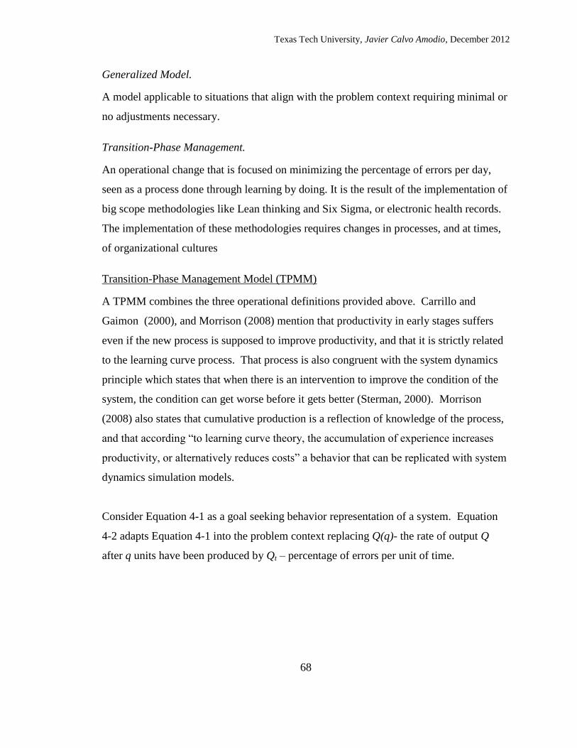
Texas Tech University, Javier Calvo Amodio, December 2012
68
Generalized Model.
A model applicable to situations that align with the problem context requiring minimal or
no adjustments necessary.
Transition-Phase Management.
An operational change that is focused on minimizing the percentage of errors per day,
seen as a process done through learning by doing. It is the result of the implementation of
big scope methodologies like Lean thinking and Six Sigma, or electronic health records.
The implementation of these methodologies requires changes in processes, and at times,
of organizational cultures
Transition-Phase Management Model (TPMM)
A TPMM combines the three operational definitions provided above. Carrillo and
Gaimon (2000), and Morrison (2008) mention that productivity in early stages suffers
even if the new process is supposed to improve productivity, and that it is strictly related
to the learning curve process. That process is also congruent with the system dynamics
principle which states that when there is an intervention to improve the condition of the
system, the condition can get worse before it gets better (Sterman, 2000). Morrison
(2008) also states that cumulative production is a reflection of knowledge of the process,
and that according “to learning curve theory, the accumulation of experience increases
productivity, or alternatively reduces costs” a behavior that can be replicated with system
dynamics simulation models.
Consider Equation 4-1 as a goal seeking behavior representation of a system. Equation
4-2 adapts Equation 4-1 into the problem context replacing Q(q)- the rate of output Q
after q units have been produced by Qt – percentage of errors per unit of time.

Texas Tech University, Javier Calvo Amodio, December 2012
69
[ ] Equation 4-2 Modified Adaptation Fucntion
where
Qt = percentage of errors per unit of time at time t
P = desired percentage of errors per unit of time
a = initial efficiency of the process
µ = process rate of adaptation = f(y1, y2, y3 … yn)
t = time t
Figure 4-1 presents a general graphical representation of Equation 4-2.
By considering systems archetypes as building blocks for a system dynamic model of
Equation 4-2, a balancing loop is the logical choice to start since it provides a goal
seeking exponential growth (positive or negative). However there are some other factors
to consider such as unintended consequences (used as damping factors) and the effects
they may have on management to change the original goal (B).
Q(t)=state of the system at time t
t
Q(0)=Initial
State
P = Desired
state
Original State
Training
Period
t0
0
Transition Period tf
f
Successful Implementation
Implementation
t
% e
rro
rs
per
day
Figure 4-1 Graphical Representation of Levy's Adaptation Function as Behavior of
Qt Over Time

Texas Tech University, Javier Calvo Amodio, December 2012
70
Therefore, a fixes that fail structure and a drifting goal structure should also be
considered. Figure 4-2 shows the resulting model represented in a causal loop diagram:
Therefore, a new mathematical model can be proposed under system dynamics
perspective.
∫
Equation4-3. Initial Transition-Phase
Management Model Until
where
Qt = percentage of errors per day
a = initial efficiency of the process = f(organizational culture, training. time)
µ = process rate of adaptation= f(experience, learning ability, feedback, time)
and
∫
{ | |
| |
Figure 4-2 Transition-Phase Management Model Causal Loop Diagram
P
P-Q(t)
a
Q(t)
+
-
+
-
DampingFactor
+
+
B
-
µ
+
-
+
Desired Percentageof Errors per Day

Texas Tech University, Javier Calvo Amodio, December 2012
71
Notice that in F (damping factor) forgetting is included as an independent variable. It
follows Morrison’s (2008) statement that forgetting is an intrinsic part of learning, but
that enough time spent with a new skill will offset the effects of forgetting.
Exploratory Study
The first task is to transform the causal loop diagram in Exhibit 3 into a stock and flow
diagram. Vensim Professional was selected to conduct the study. For this exploratory
study, the substructures a, µ and F are not developed and their behavior over time is
approximated through goal programming techniques. Figure 4-3 presents the resulting
stock and flow diagram.
Figure 4-3 Stock and Flow Diagram for of the Transition-Phase Management
Notice that table functions (lookups) are used to approximate the behaviors of a, µ and F,
as well as the B substructure (pressure to adjust the goal P). The model was expected to
produce an exponential decay behavior with dampened oscillation caused by delays in
Q(t)
µ
a
|Q(t)-P|
P
F
-
+
+
+
++
µ Lookup
a Lookup
B Lookup
Delay B
B
Po
Delay a
Delay µ
Delay F

Texas Tech University, Javier Calvo Amodio, December 2012
72
managerial decisions and information systems. Figure 4-4 presents the behavior over
time results for Qt and P-Qt.
Figure 4-4 Behavior of Qt & P-Qt Over Time
In addition, a sensitivity analysis was conducted to determine the responsiveness of the
model to changes in variable values and delay times. Figures 4-5 and 4-6 show the
behaviors of Qt and P-Qt respectively.
The model behaves within the expected bounds within expected extremes in variations of
variables levels and delay times. The results of the exploratory provide confidence to
continue developing the model as a mean to produce a generalized model to manage
transition-phases in healthcare environments.

Texas Tech University, Javier Calvo Amodio, December 2012
73
Figure 4-5 Sensitivity Results for Qt
Figure 4-6 Sensitivity Results for P-Qt
Sensitivity 1Current25% 50% 75% 95% 100%
"Q(t)"
1
0.75
0.5
0.25
00 25 50 75 100
Time (Day)
Sensitivity 1Current25% 50% 75% 95% 100%
"|Q(t)-P|"
0.8
0.58
0.36
0.14
-0.080 25 50 75 100
Time (Day)

Texas Tech University, Javier Calvo Amodio, December 2012
74
Conclusions
The proposed conceptual system dynamics model for managing transition-phases in
healthcare environments has the potential to aid healthcare managers to better determine
new process implementation strategies and enhance project implementation performance
evaluations. Management is prediction (Deming, 1998), therefore the prospect to
increase the ability to reduce uncertainty is worthy of effort. As future work, the model
proposed in this paper, will be further refined to better reflect the practice of healthcare
managers by developing second level of resolution for the a, µ and F structures. The
model can be further refined to be effective in Lean and Six Sigma settings or for other
applications of the engineering management profession.
References.
Calvo-Amodio, J., Tercero, V. G., Hernandez-Luna, A. A., & Beruvides, M. G. (2011).
"Applied Systems Thinking and Six Sigma: A Total Systems Intervention Approach".
Proceedings from the 2011American Society for Engineering Management International
Annual Conference (October 2011), Lubbock, Texas.
Carrillo, J. E., & Gaimon, C. (2000). "Improving manufacturing performance through
process change and knowledge creation". Management Science, 265-288.
Deming, W. (1998). A system of profound knowledge. The Economic Impact of
Knowledge, 161.
Flood, R. L., & Jackson, M. C. (1991). Creative problem solving: Wiley Chichester.
Hannon, B. M., & Ruth, M. (2001). Dynamic modeling: Springer Verlag.
Jackson, M. C. (2000). Systems Approaches to Management. New York: Kluwer
Academic/ Plenum Publishers.
Levy, F. K. (1965). "Adaptation in the production process". Management Science, 136-
154.
Midgley, G. (1990). "Creative methodology design". Systemist, 12(3), 108-113.
Midgley, G. (1997). "Developing the methodology of TSI: From the oblique use of
methods to creative design". Systemic Practice and Action Research, 10(3), 305-319.

Texas Tech University, Javier Calvo Amodio, December 2012
75
Morrison, J. B. (2008). "Putting the learning curve in context". Journal of Business
Research, 61(11), 1182-1190.
Sterman, J. (2000). Business dynamics: Systems thinking and modeling for a complex
world with CD-ROM: Irwin/McGraw-Hill.
Taylor, F. W. (1911). The Principles of Scientific Management. New York: Harper &
Bros.

Texas Tech University, Javier Calvo Amodio, December 2012
76
CHAPTER V
5. A GENERALIZED SYSTEM DYNAMICS MODEL FOR MANAGING
TRANSITION-PHASES IN HEALTHCARE ENVIRONMENTS
Abstract
Learning curve theory, and in particular the adaptation function have proven useful to
identify organizational learning patterns. Yet they are limited in the information they
provide in that they provide a general understanding on how long it will take to reach a
desired outcome level. If the adaptation function is to be employed to plan a transition-
phase, it should be capable of helping managers to balance quality, time and resource
cost, along with determining periods of instability and of dynamic equilibrium. The
adaptation function theory can be strengthened by combining it with systems thinking
principles and a simulation model based on system dynamics be developed as a result.
The purpose of the work presented in this paper is to develop a transition phase
management model based on a complementarist approach. Healthcare managers can
benefit from the model in two ways: 1) the model is developed into a simulation model
that possesses a user friendly interface; 2) Managers are able to forecast implementation
quality, time and resource costs, identify variables that can be modified to obtain a better
outcome by reducing periods of instability or accelerating the learning process.
Introduction
The literature points at the use of statistical process control (SPC), total quality
management (TQM), six sigma, lean thinking, and simulation as the main industrial
engineering and engineering management tools and philosophies employed in healthcare.
Many levels of success are reported, but in general, the literature suggests there have
been more partial successes and failures in implementing these methods and philosophies
than successes in healthcare and reflects on the possible causes. For instance, Benneyan

Texas Tech University, Javier Calvo Amodio, December 2012
77
(1996) offers an overview of the possible benefits that SPC could bring to healthcare. He
warns about mistakes –such as using the wrong charts and using shortcut formulas –that
can be committed if SPC tools and their application are not understood correctly.
Benneyan (1998a, 1998b, 2001) talks about control charts and their potential uses in
medical environment providing useful theoretical guidelines on how to implement them,
and analyzes their accuracy.
Callender and Grasman (Callender & Grasman, 2010) identify the following barriers to
implementation of supply chain management: Executive Support, Conflicting Goals,
Skills and Knowledge, Constantly Evolving Technology, Physician Preference, Lack of
Standardized Codes, and Limited Information Sharing. It is possible to extrapolate their
reasoning to lean thinking implementation, as they are new or foreign "industrial
engineering tools" for the medical community considering that acceptance of new ways is
always a challenge. The best practices offered can be lessened by good Lean practices
and especially with the electronic health records implementation.
Towill and Christopher (2005) advocate for the analog use of industrial logistics and
supply chain management in the National Health Service (NHS) in the United Kingdom.
They argue that material flow and pipeline concepts should be applied to the healthcare
delivery context to better match demand and the need for a more cost-effective practice.
Young (2005) proposes simulation as a tool to re-structure healthcare delivery on a
macro-level by researching patient flow, as the big hospitals go against Lean thinking
principles by promoting big queues. Young also suggests that system dynamics and
theory of constraints could work together since system dynamics is well suited to identify
bottlenecks in a process (p. 192).
Several attempts to combine methodologies, such as managerial philosophies like total
quality management, six sigma, theory of constraints, reengineering, and discrete event

Texas Tech University, Javier Calvo Amodio, December 2012
78
simulation(de Souza, 2009, p. 125) to overcome their inherent limitations have been tried,
all arising from the authors' observations that single methodologies are rarely a one-size-
fits-all solution. Yasin et al (Yasin, Zimmerer, Miller, & Zimmerer, 2002) conducted an
investigation to evaluate the effectiveness of some managerial philosophies applied into a
healthcare environment. The authors report that "it is equally clear from the data that
some tools and techniques were more difficult to implement than others" (Yasin et al.,
2002, p. 274), implying that many of the failures were due to inadequate implementations
or lack of understanding of the scope. From a systems thinking perspective, these two
types of failures in implementing a methodology are explained by the methodology's
inability to deal with very specific problem situations. This supports the point that a
complementarist industrial engineering and engineering management - systems thinking
approach can be explored by taking an atypical approach by tackling ""small"" problems,
instead of large and complex problems. This approach should convince management of
the effectiveness of a complementarist managerial philosophy using systems thinking.
Systems Thinking
Formalized systems science theory, and applied methodologies date back to the middle of
the 1900’s with the strong contributions by Ludwig von Bertalanffy’s general system
theory, Jay Forrester’s system dynamics, Russell Ackoff’s , Churchman’s and Maturana
and Varela’s autopoiesis.
The Engineering Management practice is teleologically oriented. That means that the
focus on the development of theories and their application is goal-seeking or purposeful.
Systems thinking is also teleologically oriented. Engineering management and systems
thinking are oriented to provide solutions for systems that can display choice of means
and/or ends.
[The systems age] is interested in purely mechanical systems only insofar as they
can be used as instruments of purposeful systems. Furthermore, the Systems Age
is most concerned with purposeful systems, some of whose parts are purposeful;
these are called social groups. The most important class of social groups is the

Texas Tech University, Javier Calvo Amodio, December 2012
79
one containing systems whose parts perform different functions, that have a
division of functional labor; these are called organizations. Systems-Age man is
most interested in groups and organizations that are themselves parts of larger
purposeful systems. All the groups and organizations, including institutions, that
are part of society can be conceptualized as such three-level purposeful systems.
There are three ways in which such systems can be studied. We can try to
increase the effectiveness with which they serve their own purposes, the self-
control problem; the effectiveness with which they serve the purposes of their
parts, the humanization problem; and the effectiveness with which they serve the
purposes of the systems of which they are a part, the environmentalization
problem. These are the three strongly interdependent organizing problems of the
Systems Age (Ackoff, 1973, p. 666).
When healthcare managers embark on the implementation of a EHR, or a new billing
procedure –large purposeful systems, change management is a key element of such
purposeful system.
Critical Systems Thinking
Critical systems thinking embraces five major commitments by seeking to demonstrate
critical awareness, showing social awareness, dedication to achieve human emancipation,
commitment to the development of complementary and informed development of
systems thinking methodologies at the theoretical level, and commitment to the
complementary and informed use and application of methodologies (Flood, 2010, p. 279;
Jackson, 1991, pp. 184-187).
System dynamics
System dynamics creates diagrammatic and mathematical models of feedback
processes of a system of interest. Models represent levels of resources that vary
according to rates at which resources are converted between these variables.
Delays in conversion and resulting side-effects are included in models so that
they capture in full the complexity of dynamic behaviour. Model simulation
then facilitates learning about dynamic behaviour and predicts results of various
tactics and strategies when applied to the system of interest (Flood, 2010, p.
273).
System dynamics was developed by Jay W. Forrester to model feedback loops in systems
where non-linear time dependent interactions are present. System dynamics presents a
powerful approach to modeling complex systems in accordance to what their internal

Texas Tech University, Javier Calvo Amodio, December 2012
80
structure and interactions actually are, and not in accordance to what statistics and/or
mathematical models suggest alone. Feedback is present in non-linear systems where its
components sustain complex interactions and that emergent properties arise from such
interactions. With the use of level and rate variables, it is possible to model the
interactions and feedback loops between system components. Dynamic modeling can
help identify lack of understanding of a process or system, and to identify what are the
most important variables in a process or system (Hannon & Ruth, 2001, p. 10).
Senge (2006) advocated for the use of systems thinking as the quintessential tool to
enhance the efficacy of managerial endeavors. As Forrester’s disciple, Senge’s approach
is focused on the use of system dynamics, and causal loop models.
The foundation blocks, or the common structures that describe all systems are the level
and rate equations (J.W. Forrester, 1961, 1968; 1971). Level equations result from
integrations of flows proceeding from rate inflow equations minus the integration of rate
outflows equations over time (see Equation 5-2).
In its simplest form, a rate equation depends on the state of the level variable. A rate
equation regulates, depending on the state of the level variable the flow rate (see
Equations 5-1 and 5-2).
There are two graphical tools to represent the relationships expressed in Equations 5-1
and 5-2: Causal Loop Diagrams, and Level and Rate diagrams. A causal loop diagram is
a graphical representation of the interactions between the level and rate variables in the
system. In Figure 5-1 we can see the graphical representation of Equations 5-1 and 5-2.
𝐿𝑒𝑣𝑒𝑙𝑡 ∫ 𝐼𝑛𝑓𝑙𝑜𝑤 𝑅𝑎𝑡𝑒 ∫ 𝑂𝑢𝑡𝑓𝑙𝑜𝑤 𝑅𝑎𝑡𝑒𝑛
𝑡=
𝑛
𝑡= Equation 5-2
𝑅𝑎𝑡𝑒𝑡
𝑑𝐿𝑒𝑣𝑒𝑙
𝑑𝑡 𝐼𝑛𝑓𝑙𝑜𝑤 𝑅𝑎𝑡𝑒𝑡 𝑂𝑢𝑡𝑓𝑙𝑜𝑤 𝑅𝑎𝑡𝑒𝑡 Equation 5-2

Texas Tech University, Javier Calvo Amodio, December 2012
81
The state of the level is determined by the inflow and outflow rates. The arrows
connecting the variables indicate the nature of the relationship (feedback) between them.
A positive feedback means that the rate change will be in the same direction as the
change observed in the level. A negative feedback means that the rate change will be in
the opposite direction of the change observed in the level. For instance, if the state of the
level increases, the inflow rate will decrease.
Figure 5-2 shows a Level and Rate diagram where the rate of flow and stock of goods,
materials, money, information, etc. is represented by valves and stock components. The
valves (Inflow and Outflow Rates) are controlled by the feedback received from the stock
variable (Level).
Figure 5-2 Rate and Level Diagram
LevelInflow Rate
-
Outflow Rate
+
Inflow Rate. Level.
+
-
Outflow
Rate.
+
-
Figure 5-1 Causal Loop Diagram

Texas Tech University, Javier Calvo Amodio, December 2012
82
A system dynamics model is constructed using, according to Forrester (1971; 1961,
1968) from the use of mental, written, and numerical databases (see Figure 2-8).
Different components of the model are extracted from these databases allowing the model
to replicate the real system characteristics accurately.
Barlas (1996) presents a guideline on generalized steps employed to develop a system
dynamics model:
1. Problem identification
2. Model conceptualization (construction of a conceptual model)
3. Model formulation (construction of a formal model)
4. Model analysis and validation
5. Policy analysis and design
6. Implementation
Policies, expectations and
structure,
Cause-to-effect direction
between variables
Concepts and abstractions,
Characteristics of learning
abilities, training sessions, etc.
Mental Data Base
Observation Experience
Written
Data Base
Numerical
Data Base
Figure 5-3 Mental Data Base and Decreasing Content of Written and Numerical
Data Bases

Texas Tech University, Javier Calvo Amodio, December 2012
83
The construction of a conceptual model is generally aided by the use of causal loop
diagrams.
Causal loop diagrams as mental models
Systems thinking authors such as Peter Checkland (1979a, 1979b, 1981, 1985, 1988,
1999, 2000; Checkland, Forbes, & Martin, 1990; Checkland & Scholes, 1990) and
Forrester (1961, 1971a, 1971b, 1980, 1987a, 1987b, 1991, 1992, 1994, 1995, 1999; J.
Forrester, Low, & Mass, 1974; J. Forrester & Senge, 1980) advocate for the use of mental
models to better understand, or learn about the system at hand. ‘‘The real value of
modeling is not to anticipate and react to problems in the environment, but to eliminate
the problems by changing the underlying structure of the system’’ (Sterman, 2000, pp.
655-656). Causal loop diagrams help the practitioner to uncover the underlying structure
of the system.
Efficiency, efficacy, and effectiveness of a model
When creating any model, the purpose, objectives, and benefits expected—or ends—and
the resources available – or means—must be clearly stated. Proper allocation of means
and ends can be balanced through their efficient, efficacious, and effective use within a
model. Efficiency refers to the ratio between resources used and their product (or what
the outcome is). A system is efficient if the value of the outcome or the benefit is
perceived to be higher than the value of the resources employed to produce/generate it.
An efficient model should minimize efforts while maximizing the value of outcomes.
Unfortunately when special attention is paid to the means to achieve the ends a paradox
arises. This contradiction takes place because as more resources are invested to increase
the value of the benefits, those resources become more costly, making it impossible to
reach a superior model, leading to a compromise in end quality so that the feasibility of a
model is maintained ( see Figures 5-2 and 5-4)

Texas Tech University, Javier Calvo Amodio, December 2012
84
∑
∑
Efficacy refers to the ability a system has to perform as and/or do what it is designed to
do. That is, the ends are what matters, regardless of the means employed. It is then, as
presented in the previous section, that achieving efficacy in a model results in a paradox,
but nonetheless is a highly desired characteristic.
Effectiveness refers to the alignment of what the system actually does and what the
system is supposed to do. That is, it questions the adequateness of the outcome produced
by the system. A system may be efficient and/or efficacious within its own design but
still fail to perform as desired, not effective4. Hence, a model is only effective if its
performance –regardless of its complexity—is aligned with what it is expected to do.
4 It is important to note that defining efficiency and efficacy carefully is important to approach the expected
behavior of the model.
Figure 5-4 Ratio relationship between Resources and Benefits to achieve efficiency Resources allocated
1
0 →
Efficiency
Equation 5-3 Efficiency in model
development

Texas Tech University, Javier Calvo Amodio, December 2012
85
Thus, efficiency, efficacy and effectiveness, can be used to validate a model.
Procedure depends on the purpose, so the procedure presented here is valid within that
premise.
Model Validity in a System dynamics Model
C.I. Lewis (1924), states that knowledge is probable only if our experiences and/or
interpretations of the object (what we are studying, a model for instance) and the a priori
(knowledge of the real world) –through our senses are in accordance to each other. Also
that empirical truth is possible through conceptual interpretation of the given, hence we
can have an empirical object, an imaginary construct of a reality extrapolated from our
own past experiences – an a priori. Hence, a model is a valid construct to depict a
system, a selected set of parts, interactions, and characteristics of a particular given.
Validity means “adequacy with respect to a purpose” (Barlas, 1996, p. 188). Thus, if a
model is efficient, efficacious, and effective, it is valid. However, the process of model
validation has to use semi-formal and subjective components (Barlas, 1996, pp. 183,
184). For instance, a white-box model –a system dynamics model, is built to
reproduce/predict the real world behavior, and to explain how the behavior germinates.
Ideally, the model should also suggest ways of changing the existing behavior (Barlas,
1996, p. 186).
System dynamic models are built to assess the effectiveness of alternative policies or
design strategies on improving the behavior of a given system. Therefore, “a valid model
[is] one of many possible ways of describing a real situation” (Barlas, 1996, p. 187).

Texas Tech University, Javier Calvo Amodio, December 2012
86
Barlas (1996) presents a summary of activities that can be used to validate a system
dynamics model based on a literature review (see Figure 5-5).
Figure 5-5 Overall nature and selected tests of formal model validation

Texas Tech University, Javier Calvo Amodio, December 2012
87
The structure confirmation test, requires comparison of the form of the equations of the
model against the real system (J. Forrester & Senge, 1980) as part of the mental database
and correspondence with the numerical database (as presented in Figure 5-3). The
comparison to the written database is called a theoretical structure test. It is conducted by
comparing the model equations with knowledge found in the literature (Barlas, 1996, p.
190).
The information used to validate the structure of the model is qualitative in nature, a
process similar to the validation of computer models in that the structures and data flows
are compared to the real world. It is important to test individual expressions to extreme
conditions and see if they still behave in a manner that could be expected in the real
world. Structural tests should be applied to the whole model and to subsections of the
model through simulation of normal and extreme conditions. With these tests, the
sensitivity of the model is to be uncovered, changes can be made, or at least unreliable
operation conditions are uncovered.
Learning Curve Theory
The organizational learning curve was first explored by Wright-Patterson (1936), who
observed that unit labor costs in air-frame fabrication declined with cumulative output.
From Levy (1965), Newnan, Eschenbach, and Lavelle (2004), and Yelle (1979) the
general form of the learning curve model is extracted and presented in Equation 5-4:
Equation 5-4
where
and TN = time requirement for the Nth unit of production
TInitial = time requirement for the initial unit of production
N = number of completed units (cumulative production)
θ = learning rate expressed as a decimal
1- θ = The progress ratio

Texas Tech University, Javier Calvo Amodio, December 2012
88
Relevant learning curve theory to this research work
Argote and Epple (1990) identified that organizational forgetting, employee turnover,
transfer of knowledge across products and organizations, incomplete transfer within
organizations, and economies of scale are factors that produce variability in learning
curves across organizations.
Wyer and Lundberg (1956; 1953) propose that the learning curve slope is affected by the
amount of planning put forward by management. Adler and Clark (1991) propose a
model that focuses on single -traditional experience variables and double loop learning -
two key managerial variables (engineering change and training). The authors conclude
that the learning process can vary significantly between departments and that learning can
be intensive in labor and capital intensive operations. Adler and Clark (1991) first
proposed and Lapré, Mukherjee, & Van Wassenhove (2000) confirmed that induced
learning can facilitate or disrupt the learning, stressing the importance that management
involvement has.
Adler and Clark (1991) posit that the “human learning process model begins with the
relationship between experience and the generation of data driven by that experience” (p.
270). As more data is generated, it is processed by the organization leading to the
creation of new knowledge, which in turn leads to a change in the production process.
Part of this new knowledge directly affects single-loop learning based on repetition and
on the associated incremental development of expertise. This learning helps workers or
direct laborers be more effective at their jobs. The other part of the knowledge generated
will affect the double loop learning process. Here, the learning takes place in the
management environment, where decision rules, data interpretation and data generation
are adapted to be in line with newly acquired knowledge to increment output. The
authors caution that even though a double loop-learning model is certainly a facilitator of
learning, it can disrupt knowledge either temporarily or permanently depending on

Texas Tech University, Javier Calvo Amodio, December 2012
89
management’s understanding of the learning system. It is worth noting that Adler and
Clark’s model is consistent with Stermn’s (2000) double loop-learning model presented
in Chapter 2.
Formal training and equipment replacement illustrate how managerial decision making is
improved due to a better understanding of past behavior (Yelle, 1979, p. 309), as a result
of double loop learning. Adler and Clark also express that training time should lead to
improvement in worker performance concluding that experience is also affected by
training. Learning in management is prompted by the problems encountered throughout
the production process. The new policies generated by management should result in
improved productivity. Figure 2.3 presents Adler and Clark’s learning process model.
Figure 5-6 Learning Processs Model

Texas Tech University, Javier Calvo Amodio, December 2012
90
Adaptation Function Learning Model
Levy (1965) believes that the planning process can be improved through a better
understanding of how the individual worker, as well as the firm, have historically adapted
to past learning situations. Furthermore, Levy posits that the lack of a goal seeking
behavior in traditional learning curves is not realistic. For that reason, Levy proposes an
alternative to the traditional learning curve model:
[ ] Equation 5-5
where Q(t) = percentage of errors per day at time t
P = desired rate of output expressed in errors per day
a = initial efficiency of the process expressed in percentage of
errors
µ = process rate of adaptation expressed in percentage of errors
t = cumulative time
“We suggest that the firm's cumulated experience or stock of knowledge on a particular
job at a specified time can be summarized in the stock of the product it has produced up
to that time. Thus, as the firm produces more and more of a given product, it increases its
stock of knowledge on that product and is able to come closer to the desired rate of
output” (Levy, 1965, pp. B-137).
The model assumes that there is a known, or expected, level of performance P=desired
rate of output. It also assumes that the process will start at an unwanted or initial rate of
output Q(q) with q=0. As q starts to increase, Q(q) will approach P at a rate determined
by a and µ. Levy suggests that the initial efficiency of the process (a) is an estimation of
the amount of training provided to the worker. The process rate of adaptation (µ) is a
function of different y variables that influence the rate at which an organization can learn.
The process rate of adaptation then is influenced by the experience the worker has in
similar job functions. That is, the more experienced a worker is, the faster he/she will be

Texas Tech University, Javier Calvo Amodio, December 2012
91
able to identify problems with the process and find solutions. With that, Levy suggests
that learning can happen in three different ways: autonomous learning, planned or
induced learning, and random or exogenous learning. Induced learning is influenced by
pre-planning activities such as mock runs, pre-production models, tooling determination,
etc, and by industrial engineering tools such as time and motion studies, and control
charts after the process starts. Random or exogenous learning happens when the form
gains knowledge of the process from unexpected sources such as new materials
characteristics, suppliers, government, etc. Finally, autonomous learning happens as the
worker gains more experience with the actual process and identifies ways to improve or
make more efficient his/her tasks.
Carrillo and Gaimon (2000) introduce a dynamic model to maximize profit in a process
change strategy. The model seeks to identify optimal process rate change (and when the
change should start – rate and timing for investment in process change) subject to the
ratio of cost to marginal contribution of preparation/training times to effective capacity,
cumulative knowledge, and marginal revenues produced by the new process. The authors
state that the input parameters can be adjusted to run different scenarios to select the
appropriate process change alternative.
Levy’s adaptation function (1965) introduces a goal-seeking behavior to the learning
curve body of knowledge. Equation 5-1 will generate a diminishing goal seeking
behavior until the initial percentage of errors per day reaches the desired percentage of
errors per day. Figure 5-1 presents the expected behavior over time as expressed by
Equation 5-1.
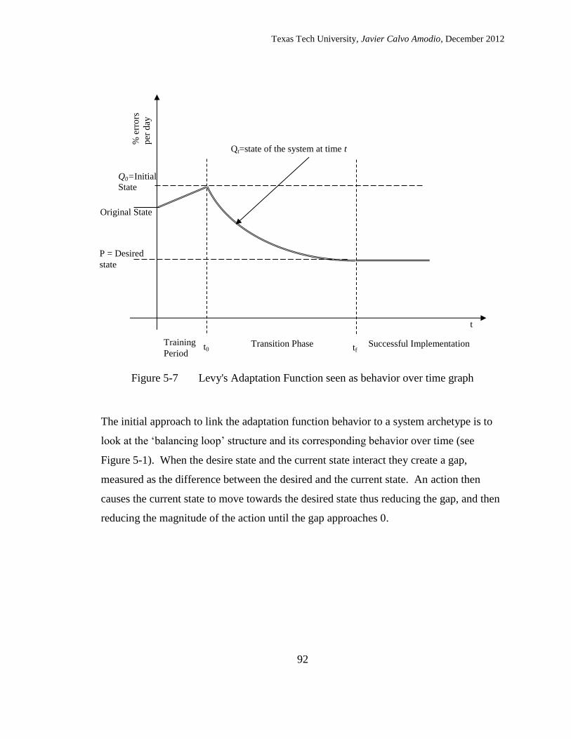
Texas Tech University, Javier Calvo Amodio, December 2012
92
The initial approach to link the adaptation function behavior to a system archetype is to
look at the ‘balancing loop’ structure and its corresponding behavior over time (see
Figure 5-1). When the desire state and the current state interact they create a gap,
measured as the difference between the desired and the current state. An action then
causes the current state to move towards the desired state thus reducing the gap, and then
reducing the magnitude of the action until the gap approaches 0.
Qt=state of the system at time t
Q0=Initial
State
P = Desired
state
Original State
Training
Period t0
Transition Phase tf Successful Implementation
t
% e
rro
rs
per
day
Figure 5-7 Levy's Adaptation Function seen as behavior over time graph

Texas Tech University, Javier Calvo Amodio, December 2012
93
At first glance, the ‘balancing loop’ appears to be a good fit to the behavior over time
described in Figure 5-1. However, in reality a transition-phase will not occur without
glitches or inconsistencies – a limitation that the adaptation function possesses. For
instance, the balancing loop ignores the effects of factors like forgetting, employee
absenteeism, different levels of experience, varying learning abilities, pressure to adjust
the goals, and pressure to complete the project on time.
The ‘drifting goals’ archetype considers negative effects from low levels of experience,
and learning abilities which may result in changes on deadlines, or target state. Figure 5-
3 presents the ‘drifting goals’ archetype using causal loops.
Figure 5-8 ‘Balancing Loop’ Causal Loop Diagram and Behavior Over Time
Graph
Desired State Gap
ActionCurrent State
+-
+
+
Current State
Desired State Gap
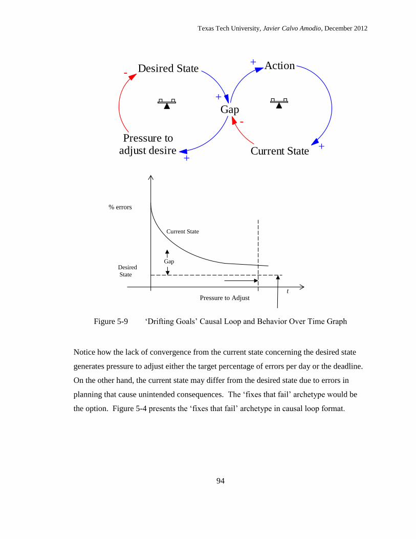
Texas Tech University, Javier Calvo Amodio, December 2012
94
Figure 5-9 ‘Drifting Goals’ Causal Loop and Behavior Over Time Graph
Notice how the lack of convergence from the current state concerning the desired state
generates pressure to adjust either the target percentage of errors per day or the deadline.
On the other hand, the current state may differ from the desired state due to errors in
planning that cause unintended consequences. The ‘fixes that fail’ archetype would be
the option. Figure 5-4 presents the ‘fixes that fail’ archetype in causal loop format.
Desired State
Gap
Action
Current State
+
-
+
+Pressure to
adjust desire
-
+
% errors
t
Current State
Desired
State
Gap
Pressure to Adjust

Texas Tech University, Javier Calvo Amodio, December 2012
95
The ‘drifting goals’ and ‘fixes that fail’ archetypes provide more complete solutions than
the ‘balancing loop’ archetype and/or the adaptation function alone. However, if used
separately they provide an incomplete solution. Figure 5-5 presents the combination of
the ‘balancing loop’ with the ‘drifting goals’ and ‘fixes that fail’ archetypes. This new
Figure 5-10 ‘Fixes that Fail’ Causal Loop and Behavior Over Time Graphs
Desired State
Gap
Action
Current State
+
-
+
+
UnintendedConsequences
+
-
Current State
Desired
State
Gap
% e
rro
rs
t
Current State
Desired
State
Gap
%
erro
rs
t
Current State
Desired
% of errors
Gap
% e
rro
rs
t

Texas Tech University, Javier Calvo Amodio, December 2012
96
structure derived from a complementarist approach is called the adaptation function
causal loop.
The action variable is a result of learning ability or efficiency of the process and process
rate of adaptation. The authors propose efficiency of the process and process rate of
adaptation as actions and autonomous learning (lack of) as unintended consequences.
Levy (1965) suggests that there are three types of adaptation processes. The first one is
planned or induced learning that impacts directly the potential efficiency of the process.
The second one is random or exogenous learning, resulting from information received
about the process that could not be anticipated or planned for and it impacts the process
rate of adaptation. The third type is autonomous learning, which results from planning
and on-the-job learning mitigating the effects of unintended consequences..
Efficiency of the Process
Levy posits that the less the firm pre-plans, the more opportunity there would be for the
firm to improve its operation. He suggests that the amount of planning should be
inversely related to the rate of learning (Levy, 1965, p. B139). However based on
Figures 5-2 to 5-5 it is possible to conclude that the less the firm plans (efficiency of the
process) the bigger the gap will be and the larger the unintended consequences will be.
Desired State
Gap
Action
Current State
+
-
+
+
UnintendedConsequences
+
-
Pressure toAdjust Desire
-
+
Figure 5-11 Adaptation Function Causal Loop Diagram

Texas Tech University, Javier Calvo Amodio, December 2012
97
Therefore factors that can be controlled before the new process implementation and that
are endogenous to the organizational structure such as training, business seasonality,
organizational culture and technology available are determine the efficiency of the
process.
Process rate of adaptation
The process rate of adaptation is composed by variables that are affect the
implementation process during the implementation process such as learning ability,
employee’s experience, and education. That is, the faster the organization adapts to
changes, the smoother the implementation will be (it will reduce the oscillation) and the
faster it will converge with the desired state.
Unintended consequences (or damping factors)
Autonomous learning is according to Levy (1965) a result of the efficiency of the process
and the process rate of adaptation. Autonomous learning will be considered as negative
unintended consequences; that is, the less autonomous learning there is, the bigger the
effect of the unintended consequences will be.
Research Question
Thus, the concern addressed in this research is: Can a generalized system dynamics
transition-phase management model be developed by combining adaptation function
theory and system dynamics?
Model Development – System Identification
Development of the substructures requires the development of operational definitions for
each factor. Each factor is evaluated, based on their operational definition, in accordance
to a general rubric (see Table 5-1)

Texas Tech University, Javier Calvo Amodio, December 2012
98
Table 5-1 General Rubric to Evaluate Factors
Grade 1 2 3 4 5
Meaning Very Poor or
non-existent Poor Average
Above
average
Superior or
excellent
Managers wishing to evaluate their organization’s capacity to implement a new process
need to grade each one of the factors in accordance to their operational definitions as
suggested in the general rubric (Table 5-1). Grades do not have to be integers.
Efficiency of the Process substructure (a)
In this sub-structure the factors that have an effect on the efficiency of the organization to
implement new processes are considered. The factors were selected in accordance to
mental data bases (see Figure 2-8) after informal interviews with healthcare managers. It
is worth noting that in independent interviews, the managers listed the same factors.
The efficiency of the process substructure is designed to calculate the magnitude of its
impact to the current percentage of errors per day (Qt) and to determine delays resulting
from the factors values. Figure 5-1 presents the resulting structure:

Texas Tech University, Javier Calvo Amodio, December 2012
99
Adequacy of Technology in Company
This factor identifies how efficient, efficacious and effective is the current technology
(computing, software, communications) with regards to the company’s operations. For
instance, a grade of 1 may indicate that not even the most basic tasks are supported
correctly by the current technological standards. A grade of 5 may represent that there is
room for improvement, but all basic operations are satisfied with current standards. A
grade of 10 may indicate that all technology is state-of-the-art and the company is leader
in operations and standards.
Adequacy of Technology for Project
Identifies how efficient, efficacious and effective is the current technology (computing,
software, communications) with regards to the proposed new process requirements. For
instance, a grade of 1 may indicate that not even the most basic tasks would be supported
correctly by the current technological standards. A grade of 5 may represent that there is
room for improvement, but all basic operations would be satisfied with current standards.
A grade of 10 may indicate that all technology is state-of-the-art and the company is
Adequacy ofTechnology
Does Project DemandChanges in Technology?
BusinessSeasonality
OrganizationalCulture - Weighted
TrainingFrequency
TrainingDuration
+
Adequacy ofTechnology in
Company
Adequacy ofTechnology for
Project +
+
Lookup forATP
+
a substructure+
+++ +
Delay forSubstructure a
Maximum DelayExpected for aSubstructure
OrganizationalCulture
Figure 5-12 Efficiency of the Process Sub-structure (a)

Texas Tech University, Javier Calvo Amodio, December 2012
100
leader in operations and standards. Note: both technology factors are evaluated on a
scale of 1-10.
Training Frequency
Training frequency refers to how close from each other are held the training sessions. A
grade of 1 represents a daily training schedule. A grade of 2 represents a 3 day a week
training schedule. A grade of 3 represents 2 days a week training schedule. A grade of 4
represents 1 day per week training schedule. And a grade of 5 represents less than one
day a week training schedule.
Training Duration
Training duration refers to the length of each training session. A grade of 1 represents a
session shorter than 1 hour. A grade of 2 represents a session of 1 hour. A grade of 3
represents a session of 1.5 hours. A grade of 4 represents a session of 2 hours. A grade of
5 represents a session longer than 2 hours.
Business Seasonality
Business seasonality refers to the state of the business cycle in a healthcare provider, i.e.
if it is flu season, budgeting season, etc. A grade of 1 refers to a very busy business cycle
(i.e. flu season, financial reports) and a grade of 5 represents a slow business cycle
(meaning priority can be placed to the new process implementation).
Organizational Culture
Organizational culture refers to the flexibility and organizational climate in the
organization with respect to new process adoption. A grade of 1 represents a very poor
organizational culture. A grade of 5 indicates excellent organizational culture.
Maximum delay expected
Managers should make an assumption on what they expect to be the longest delay that
could be caused by the factors within the structure.
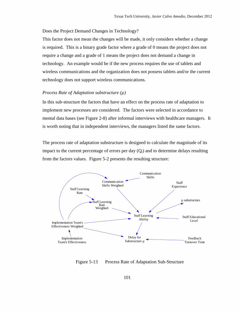
Texas Tech University, Javier Calvo Amodio, December 2012
101
Does the Project Demand Changes in Technology?
This factor does not mean the changes will be made, it only considers whether a change
is required. This is a binary grade factor where a grade of 0 means the project does not
require a change and a grade of 1 means the project does not demand a change in
technology. An example would be if the new process requires the use of tablets and
wireless communications and the organization does not possess tablets and/or the current
technology does not support wireless communications.
Process Rate of Adaptation substructure (µ)
In this sub-structure the factors that have an effect on the process rate of adaptation to
implement new processes are considered. The factors were selected in accordance to
mental data bases (see Figure 2-8) after informal interviews with healthcare managers. It
is worth noting that in independent interviews, the managers listed the same factors.
The process rate of adaptation substructure is designed to calculate the magnitude of its
impact to the current percentage of errors per day (Qt) and to determine delays resulting
from the factors values. Figure 5-2 presents the resulting structure:
StaffExperience
Staff EducationalLevel
Implementation Team'sEffectiveness Weighted
Staff LearningAbility
CommunicationSkills Weighted
FeedbackTurnover Time
µ substructureStaff Learning
RateWeighted
Delay forSubstructure µ
ImplementationTeam's Effectiveness
Staff LearningRate
CommunicationSkills
Figure 5-13 Process Rate of Adaptation Sub-Structure

Texas Tech University, Javier Calvo Amodio, December 2012
102
Feedback Turnover Time
Feedback turnover time refers to how long does it take for the implementation team to
address inquiries from end users. This is an estimation that has to be made with the best
knowledge available. The value is to be expressed in days. The rubric is not required for
this factor.
Implementation Team Effectiveness
Measures how experienced, cohesive and dynamic the implementation team is. It is
measured with respect to the expected impact it can have on the transition phase. A
grade of 1 represents a very poor or negative impact and a grade of 5 represents an
excellent positive impact.
Staff Learning Rate
Staff learning rate refers to the overall learning ability of the staff. A grade of 1
represents a very poor learning rates and a grade of 5 represents excellent learning rates.
It is to be expressed as an average of all involved staff in the new process operations.
Communication Skills
Communication skills refer to the organization’s personnel ability and willingness to
communicate with each other. A grade of 1 represents very poor communication skills
and a grade of 5 represents excellent communication skills.
Staff Experience
Staff experience refers to the level of experience that the staff possesses both in
professional jobs and in a job related to their current one. A grade of 1 indicates no at all
and a grade of 5 indicates a high level of relevant experience.

Texas Tech University, Javier Calvo Amodio, December 2012
103
Staff Educational Level
Staff educational level refers to the minimum and maximum academic levels achieved by
the staff. A grade of 1 indicates incomplete K-12 education. A grade of 5 indicates
graduate degrees.
Feedback Turnover Time
Refers to the expected normal time to receive, acknowledge and resolve issues. It is
expressed in days.
Damping Factors Sub-Structure
The damping factors sub-structure calculates the magnitude of a unexpected
consequences based on the existence of standard operating procedures (SOPs) and the
effect of forgetting. In the main structure it reacts to the values generated by the
efficiency of the process and process rate of adaptation sub-structures.
Figure 5-14 Damping Factors Sub-Structure
Forgetting
Existence ofSOPs
<TrainingDuration>
<TrainingFrequency>
F substructure
-
<FeedbackTurnover Time>
<a substructure>Expected %Forgetting
Delay forSubstructure F
<asubstructure>
<µsubstructure>

Texas Tech University, Javier Calvo Amodio, December 2012
104
Forgetting
It is an estimation of the percentage of training and process details expected to be
forgotten by the process users.
Existence of SOPs (Standard Operating Procedures)
A grade of 0 represents no presence of SOPs for the new process. A grade of 1
represents existence of SOPs for the new process.
All factors were determined based on Figure 5-3 approach using as mental database the
interviews with the managers and by identifying the five Ms+E (Measurements,
Materials, Personnel, Environment, Methods and Machines) from Ishikawa’s fishbone
diagram and adapting them to the particular activities within a healthcare environment.
The written database from the literature review validated the observations from the
managers and their interpretations of Ishikawa’s five Ms+E.
Model Validation - Simulation
In this section, a sensitivity analysis is presented varying the ranges of inputs of different
sets of variables and to all input variables at once and their effects to the initial state (Q0),
current state (Qt), gap (Q0-P0), all efficiency of the process (a) factors, and all process
rate of adaptation (µ) factors. Table 5-2 presents a relation between the parameters being
tested and the corresponding Figure according to the function employed.

Texas Tech University, Javier Calvo Amodio, December 2012
105
Table 5-2 Relation of Validation Tests, Parameters and Corresponding
Figure
Test
# Parameters
Figure
Uniform Triangular
1 P0 and Q0 5-4
2 All sub-structures factors 5-5
3 All sub-structures factors, P0 and Q0 5-6 5-9, 5-11,
5-13
4 Pessimistic scenario with all sub-structures
factors set at 1
No D
sitr
ibu
tion
5-7 (a) 5-8
5 Moderate scenario with all sub-structures factors
set at 3 5-7 (b) 5-10
6 Optimistic scenario with all sub-structures
factors set at 5 5-7 (c) 5-12
The tests were performed using the built in sensitivity analysis in Vensim Professional
software. Each parameter possible value is explored either using a uniform or a
triangular distribution. 10,000 replications were conducted for each sensitivity test. A
time frame of 90 days was set.
Extremes tests
In this section, Figures 5-15 to 5-18 show the results of sensitivity analysis by testing the
model throughout its extreme values. The tests serve to investigate if the model behaves
in unexpected ways, and as it can be observed it does not.
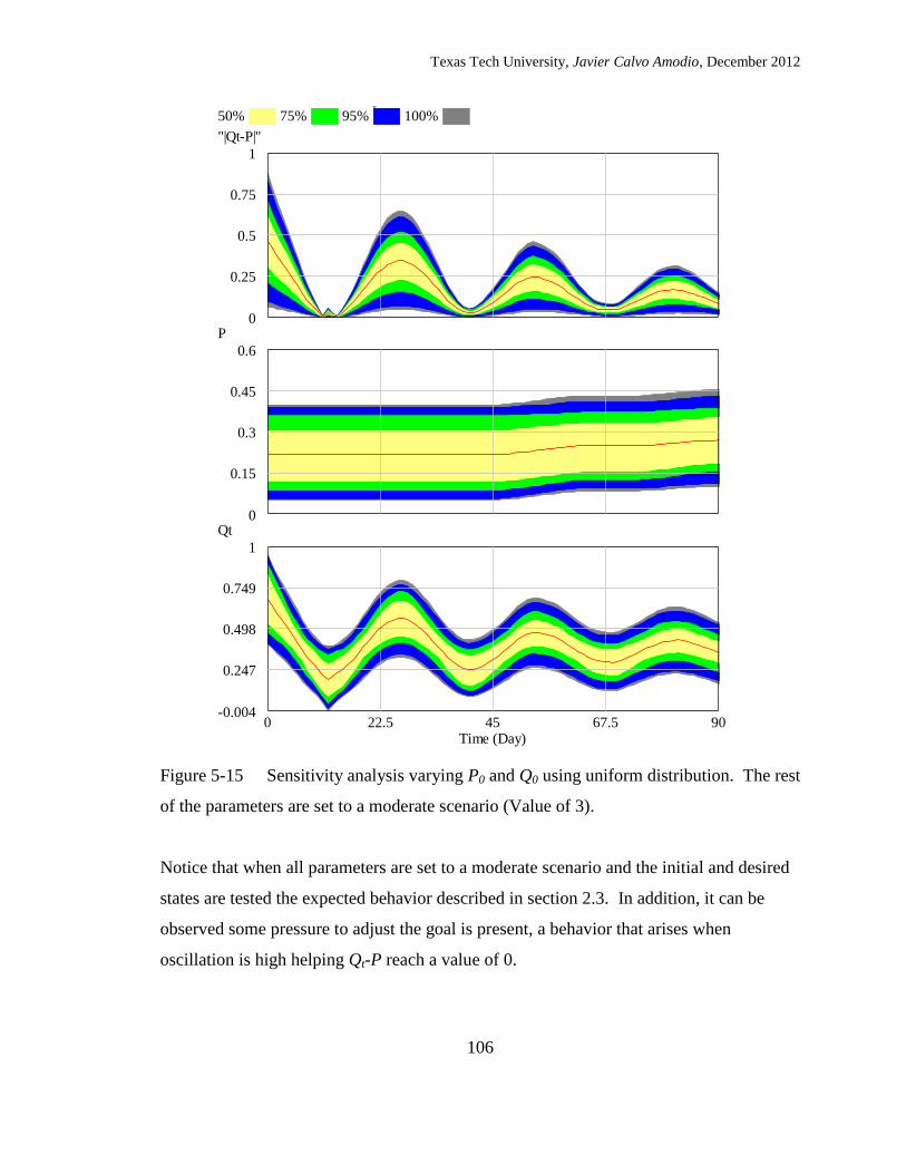
Texas Tech University, Javier Calvo Amodio, December 2012
106
Figure 5-15 Sensitivity analysis varying P0 and Q0 using uniform distribution. The rest
of the parameters are set to a moderate scenario (Value of 3).
Notice that when all parameters are set to a moderate scenario and the initial and desired
states are tested the expected behavior described in section 2.3. In addition, it can be
observed some pressure to adjust the goal is present, a behavior that arises when
oscillation is high helping Qt-P reach a value of 0.
General Model - Sensitivity 150% 75% 95% 100%
"|Qt-P|"
1
0.75
0.5
0.25
0P
0.6
0.45
0.3
0.15
0Qt
1
0.749
0.498
0.247
-0.0040 22.5 45 67.5 90
Time (Day)

Texas Tech University, Javier Calvo Amodio, December 2012
107
Figure 5-16 Sensitivity analysis varying all factors in substructures using a random
uniform distribution P0 and Q0 fixed.
Notice how when all factors are randomly varied, the distribution of possible outcomes
becomes wider and the pressure to adjust the goal (P) is incremented substantially. In
this test it is possible to observe that all possible behaviors that the model can generate
are consistent with section 2.3. The center line indicates the average of all 10,000 runs.
General Model - Sensitivity 250% 75% 95% 100%
"|Qt-P|"
0.6
0.45
0.3
0.15
0P
0.4
0.35
0.3
0.25
0.2Qt
1
0.7
0.4
0.1
-0.20 22.5 45 67.5 90
Time (Day)

Texas Tech University, Javier Calvo Amodio, December 2012
108
Figure 5-17 Sensitivity analysis varying all factors in substructures and P0 and Q0
using a random uniform distribution.
All factors plus P0 and Q0 are varied throughout the whole range of values in accordance
to section 2.3 depicting all possible values the model can generate showing no undesired
behavior.
General Model - Sensitivity 350% 75% 95% 100%
"|Qt-P|"
2
1.5
1
0.5
0P
0.6
0.45
0.3
0.15
0Qt
2
1
0
-1
-20 22.5 45 67.5 90
Time (Day)

Texas Tech University, Javier Calvo Amodio, December 2012
109
(a) Pessimistic Scenario –
Value of 1
(b) Moderate Scenario –
Value of 3
(c) Optimistic Scenario –
Value of 5
Figure 5-18 Discrete analysis setting all factors in to a pessimistic (a), moderate (b),
and optimistic (c) scenarios with P0=10% and Q0=50%.
As can be seen the behaviors over-time depicted in Figures 5-18 a, b and c are consistent
with those from Figure 5-15 to 5-17.
Current
"|Qt-P|"
0.6
0.45
0.3
0.15
0P
0.4
0.3
0.2
0.1
0Qt
0.8
0.6
0.4
0.2
00 50 100
Time (Day)
Current
"|Qt-P|"
0.6
0.45
0.3
0.15
0P
0.2
0.175
0.15
0.125
0.1Qt
0.8
0.6
0.4
0.2
00 50 100
Time (Day)
Current
"|Qt-P|"
0.6
0.45
0.3
0.15
0P
0.2
0.175
0.15
0.125
0.1Qt
0.8
0.6
0.4
0.2
00 50 100
Time (Day)

Texas Tech University, Javier Calvo Amodio, December 2012
110
Substructures effect on Qt
In this section a sensitivity analysis is run just varying separately the factors of each
structure.
Figure 5-19 a substructure impact on Qt
General Model a Substructure50% 75% 95% 100%
"Qt-P"
0.6
0.4350
0.27
0.105
-0.06P
1
0.75
0.5
0.25
0Qt
0.8
0.6
0.4
0.2
00 22.5 45 67.5 90
Time (Day)

Texas Tech University, Javier Calvo Amodio, December 2012
111
Figure 5-20 µ substructure impact on Qt
General Model µ substructure50% 75% 95% 100%
"Qt-P"
1
0.5
0
-0.5
-1P
0.4
0.35
0.3
0.25
0.2Qt
0.8
0.4
0
-0.4
-0.80 22.5 45 67.5 90
Time (Day)

Texas Tech University, Javier Calvo Amodio, December 2012
112
General Model F substructure
50% 75% 95% 100%
"Qt-P"
0.6
0.43
0.26
0.09
-0.08P
0.4
0.35
0.3
0.25
0.2Qt
0.8
0.6
0.4
0.2
00 22.5 45 67.5 90
Time (Day)
Figure 5-21 F substructure impact on Qt
Figures 5-20, 5-21 and 5-22 demonstrate that a, µ, and F substructures do have an effect
on the percentage of errors per day (Qt). Note that if there is an increase in P, B is having
an effect it means the goal Qt-P 0 is not being met therefore inducing pressure to
adjust the goal.

Texas Tech University, Javier Calvo Amodio, December 2012
113
Bias analysis
Next sensitivity simulations using triangular distributions to vary the factor values in
accordance to a pessimistic, moderate and optimistic scenario (much like Figure 518) are
presented.
Figure 5-22 Sensitivity analysis using triangular distribution with peak set to
pessimistic scenario varying all factors in substructures (value of 1).
General Model - Sensitivity 3 - Triangular - All - Value 550% 75% 95% 100%
"|Qt-P|"
1
0.75
0.5
0.25
0P
0.6
0.45
0.3
0.15
0Qt
2
1.4
0.8
0.2
-0.40 22.5 45 67.5 90
Time (Day)

Texas Tech University, Javier Calvo Amodio, December 2012
114
Figure 5-23 Sensitivity analysis using triangular distribution with peak set to
pessimistic scenario varying all factors in substructures (value of 1) plus varying P0 and
Q0.
Figures 5-23 and 5-24 portray a sensitivity analysis with a bias towards a pessimistic
scenario using a triangular distribution.
General Model - Sensitivity 3 - Triangular - All - Value 550% 75% 95% 100%
"|Qt-P|"
2
1.5
1
0.5
0P
0.8
0.6
0.4
0.2
0Qt
4
2.85
1.7
0.55
-0.60 22.5 45 67.5 90
Time (Day)

Texas Tech University, Javier Calvo Amodio, December 2012
115
Figure 5-24 Sensitivity analysis using triangular distribution with peak set to moderate
scenario varying all factors in substructures(value of 3).
General Model - Sensitivity 3 - Triangular - All - Value 550% 75% 95% 100%
"|Qt-P|"
1
0.75
0.5
0.25
0P
0.6
0.45
0.3
0.15
0Qt
2
1.4
0.8
0.2
-0.40 22.5 45 67.5 90
Time (Day)

Texas Tech University, Javier Calvo Amodio, December 2012
116
Figure 5-25 Sensitivity analysis using triangular distribution with peak set to moderate
scenario varying all factors in substructures (value of 3) plus P0 and Q0.
Figures 5-25 and 5-26 portray a sensitivity analysis with a bias towards a moderate
scenario using a triangular distribution.
General Model - Sensitivity 3 - Triangular - All - Value 550% 75% 95% 100%
"|Qt-P|"
2
1.5
1
0.5
0P
0.6
0.45
0.3
0.15
0Qt
2
1
0
-1
-20 22.5 45 67.5 90
Time (Day)

Texas Tech University, Javier Calvo Amodio, December 2012
117
Figure 5-26 Sensitivity analysis using triangular distribution with peak set to
optimistic scenario (value of 5)
General Model - Sensitivity 3 - Triangular - All - Value 550% 75% 95% 100%
"|Qt-P|"
1
0.75
0.5
0.25
0P
0.4
0.35
0.3
0.25
0.2Qt
2
1.4
0.8
0.2
-0.40 22.5 45 67.5 90
Time (Day)

Texas Tech University, Javier Calvo Amodio, December 2012
118
Figure 5-27 Sensitivity analysis using triangular distribution with peak set to
optimistic scenario (value of 5) including P0 and Q0.
Figures 5-27 and 5-28 portray a sensitivity analysis with a bias towards an optimistic
scenario using a triangular distribution.
General Model - Sensitivity 3 - Triangular - All - Value 550% 75% 95% 100%
"|Qt-P|"
2
1.5
1
0.5
0P
0.6
0.45
0.3
0.15
0Qt
2
1
0
-1
-20 22.5 45 67.5 90
Time (Day)

Texas Tech University, Javier Calvo Amodio, December 2012
119
Conclusions
Can the model developed serve as a generalized system dynamics transition-phase
management model? Figures 5-4 to 5-15 present evidence to answer affirmatively the
question.
Dampened Oscillation
In detail, Figure 5-4 tests the effects that varying the initial state of the system or initial
percentage of errors per day Q0, desired percentage of errors per day P0 separately and
then together have on the percentage of errors per day, pressure to adjust the goal and the
gap (Qt-P). The rest of the parameters are set to a moderate scenario (mid values
throughout their range). It shows that varying initial percentage of errors per day Q0 and
desired percentage of errors per day P0 create oscillation and that the bigger the
difference between Q0 and P0 the larger the oscillation is and the smaller the effect of the
dampening is. That combination produces pressure to adjust the goal when the
oscillation is larger and the effects of the dampening are small. For managers, it means
that in order to reduce instability of the process, it is necessary to reduce the gap between
Q0 and P0 by either reducing Q0 or by increasing P0.
Path Forecasting
Figure 5-5 presents a simulation varying all factors but Q0 and P0 with their gap set to be
40% of errors per day. The rest of the factors are varied using uniform distribution
assuming same probabilities for each of their values to occur. The results show the full
range of paths that a process can take assuming a moderate gap size (Q0 and P0). When
factors combine in their highest values the dynamic equilibrium state is reached fast, and
when factors combine in their lowest values the process can completely go out of control.
Figure 5-6 presents the full potential range when all factors are varied uniformly. The
range of paths is increased as the amplitude of the oscillation. Managers can understand
periods of instability (non-dynamic equilibrium) and expected performance (path) of the

Texas Tech University, Javier Calvo Amodio, December 2012
120
implementation process. As an illustration, Figure 5-7 presents specific cases where all
factors are set to pessimistic (5-7a), moderate (5-7b) and optimistic scenarios (5-7c).
Effects of the substructures on the percentage of errors per day
Figures 5-8, 5-9 and 5-10 explore the effects that each of the substructures a (efficiency
of the process), µ (process rate of adaptation) and F (damping factors) have on Qt
(percentage of errors per day). Figure 8 shows how the efficiency of the process has a
bigger effect on the amplitude and dampening of the oscillation, an effect that is
consistent with the definition of efficiency of the process provided in the introduction
section. It means that managers can invest more in their organizational structure to
minimize instability and/or to accelerate the rate at which the new process can reach
dynamic equilibrium.
Figure 5-9 shows how the implementation of the new process path can vary; if the
parameters are set at a pessimistic scenario the path will move further away from the
desired state. Conversely, if the parameters are set to an optimistic scenario then the path
will converge faster with the desired state (it will reach dynamic equilibrium faster).
Figure 5-10 shows the effects that the damping factors have on the percentage of errors
per day. If the parameters are set to a pessimistic scenario, then the effect of the
shortages in a and µ are accentuated creating big deviations and large delays on the
response times.
Model behavior in pessimistic, moderate and optimistic scenarios
Figures 5-11 to 5-16 present the results of sensitivity simulations varying all parameters,
and all parameters minus Q0 and P0 using a triangular distribution setting the peak at
pessimistic, moderate and optimistic scenarios. Odd numbered Figures show simulations

Texas Tech University, Javier Calvo Amodio, December 2012
121
with all parameters but Q0 and P0 and even numbered Figures show simulations varying
all parameters.
Figures 5-11, 5-13 and 5-15 show the distribution density of the paths using all
parameters sans Q0 and P0 being consistent with the bias incorporated into the simulation
by the triangular distribution. Figures 5-12, 5-14 and 5-16 show the show the distribution
density of the paths using all parameters being consistent with the bias incorporated into
the simulation by the triangular distribution. The latter means that the model is accurate
in predicting the paths, periods of instability and when the dynamic equilibrium is
expected to be reached.
Future Work
The results from the sensitivity simulations are encouraging. The model behaves
according to the theory and is capable of forecasting different behaviors arising from all
factors’ possible combinations.
The model still requires to be tested in real life projects to better assess its accuracy and
reliability. For that, future work requires the application of the model in real world
scenarios exploring projects that present different completion lengths and differences
between Q0 and P0.
References
Adler, P.S., & Clark, K.B. (1991). Behind the learning curve: A sketch of the learning
process. Management Science, 267-281.
Argote, L., & Epple, D. (1990). Learning curves in manufacturing. Science, 247(4945),
920.
Benneyan, J.C. (1996). Using statistical process control (SPC) to measure and improve
health care quality.
Benneyan, J.C. (1998a). Statistical quality control methods in infection control and
hospital epidemiology, part I: Introduction and basic theory. Infection Control and
Hospital Epidemiology, 194-214.

Texas Tech University, Javier Calvo Amodio, December 2012
122
Benneyan, J.C. (1998b). Statistical quality control methods in infection control and
hospital epidemiology, Part II: chart use, statistical properties, and research issues.
Infection Control and Hospital Epidemiology, 265-283.
Benneyan, J.C. (2001). Number-between g-type statistical quality control charts for
monitoring adverse events. Health Care Management Science, 4(4), 305-318.
Callender, C., & Grasman, S.E. (2010). Barriers and Best Practices for Material
Management in the Healthcare Sector. Engineering Management Journal; EMJ,
22(4), 11.
Carrillo, J.E., & Gaimon, C. (2000). Improving manufacturing performance through
process change and knowledge creation. Management Science, 265-288.
de Souza, L.B. (2009). Trends and approaches in lean healthcare. Leadership in Health
Services, 22(2), 121-139.
Lapré, M.A., Mukherjee, A.S., & Van Wassenhove, L.N. (2000). Behind the learning
curve: Linking learning activities to waste reduction. Management Science, 597-
611.
Levy, F.K. (1965). Adaptation in the production process. Management Science, 136-154.
Lundberg, R.H. (1956). Learning Curve Theory as Applied to Production Costs. SAE
Journal, 64(6), 48-49.
Newnan, D.G., Eschenbach, T., & Lavelle, J.P. (2004). Engineering economic analysis:
Oxford Univ Pr.
Towill, DR, & Christopher, M. (2005). An evolutionary approach to the architecture of
effective healthcare delivery systems. Journal of Health, Organisation and
Management, 19(2), 130-147.
Wright-Patterson, TP. (1936). Factors Affecting the Cost of Airplanes. Journal of
Aeronautical Sciences, 3(4), 122-128.
Wyer, R. (1953). Learning curve helps Figure profits, control costs. National Association
of Cost Accountants Bulletin, 35 (4), 490, 502.
Yasin, M.M., Zimmerer, L.W., Miller, P., & Zimmerer, T.W. (2002). An empirical
investigation of the effectiveness of contemporary managerial philosophies in a
hospital operational setting. International Journal of Health Care Quality
Assurance, 15(6), 268-276.
Yelle, L.E. (1979). The learning curve: Historical review and comprehensive survey.
Decision Sciences, 10(2), 302-328.
Young, T. (2005). An agenda for healthcare and information simulation. Health Care
Management Science, 8(3), 189-196.

Texas Tech University, Javier Calvo Amodio, December 2012
123
CHAPTER VI
6. APPLICATION OF TRANSITION-PHASE MANAGEMENT MODEL IN BILLING
HEALTHCARE ENVIRONMENT
Abstract
The implementation of an electronic health records system requires changes in processes,
which in turn require management of such transition-phases. Electronic health records
systems implementations are composed of various subsystems such as medical, clerical,
administrative and billing. The complexity of each an electronic health records
implementation in each of these subsystems is affected by project length, and size
measured by the number of places it is deployed and the timing of each deployment. An
evaluation of the transition-phase management model on a long term multi-phase
electronic health records implementation process is presented. Analysis of the adequacy
and accuracy of the model is provided and guidelines for interpretation are suggested.
Introduction
The transition-phase management model, developed by Calvo-Amodio, et. al. (201X)
present a method to evaluating the capabilities of an organization to implement an
electronic health records system according to their current state and resources available.
In this paper, the transition-phase management model is evaluated against a multi-phase
long term electronic health records system implementation project.
Background
Attempts to better manage healthcare organizations have been made using lean thinking.
De Souza (2009) proposes a taxonomy of the application of Lean thinking on healthcare
through a literature review. De Souza divides the lean healthcare literature into two
categories: case studies and theoretical, concluding that lean healthcare appears to be an

Texas Tech University, Javier Calvo Amodio, December 2012
124
effective way to better healthcare organizations. He argues that lean is a better fit to
healthcare as it is more adaptable in healthcare settings than other management
philosophies, the potential it has to empower staff along with the concept of continuous
improvement. He states that it “is believed that lean healthcare is gaining acceptance not
because it is a ‘new movement’ or a ‘management fashion’ but because it does lead to
sustainable results” (p. 122). Lean healthcare is a relatively new concept, as can be seen
in the history of lean thinking in a Figure De Souza adapted from Laursen et al. (2003, p.
3) (Figure 2-1).
Figure 6-1. The appearance of lean healthcare.
As can observed in Figure 6-1 (de Souza, 2009, p. 123), lean healthcare is relatively a
new practice and research area. As would be expected, there is still much work to be
done. Berwick, Kabcenell, & Nolan (2005) mention that lean healthcare, although is on
the right path, still has a long way to go to be comparable with mainstream applications
of lean thinking.

Texas Tech University, Javier Calvo Amodio, December 2012
125
De Souza concludes that the majority of the literature is theoretical, with 30% being
speculative and less than 20% being methodological in nature, and expects the field to
grow in the near future.
Action Research
Action research “results from an involvement with members of an organization over a
matter which is of genuine concern to them” (Eden & Huxham, 1996, p. 75). Action
research was developed for research in management sciences. However, it should also
provide a great tool for industrial engineering and engineering management research
where a significant part of the focus on research is on problem solving applications.
Action research is adequate for situations when the application of some knowledge (new
or existing) into a particular problem context can have wider research consequences that
are worth investigating. A practitioner can apply an industrial engineering and
engineering management tool to a particular system. However, without a systemic
thinking mode, the solution may end up causing some undesired effects within the same
system and/or on a seemingly unrelated system. This can bring a methodological debate
between practitioners and researcher as to how to address such vicissitudes.
Rosmulder et al (2011) explore the use of simulation models while conducting action
research. They conclude that “the design of the simulation model would play a crucial
role in the AR experiment” (p. 400). They stress that in order to have all the stakeholders
willing to take action during the action research process; they should accept the model
and have confidence in the structure and outcomes it generates.
Problem Context
In order to complete the validation of the model, it has to be compared against real world
data. In this experiment focus is placed on a multiple-phase long-term project. Data
about errors per day committed by end users of a new electronic health records process
was provided by a local healthcare center.

Texas Tech University, Javier Calvo Amodio, December 2012
126
Oral in-person sessions were conducted resulting in agreement of the healthcare center to
provide qualitative and quantitative data regarding the implementation process. All
identifiers from personnel related data were removed by the data providers, eliminating
the possibility for the researcher to relate data to any staff member. The procedure for
data collection and a handout containing the major steps are presented below.
Data Collection Procedure
Data was obtained through interviews with the process change manager. Table 6-1
presents a summary of the data required:
Table 6-1 Summary of Data
Variable Output Value Delivery
Format
Adequacy of Technology in Company 1-10
Fill-in format
to be provided
to managers.
Refers to how well does the current technology (computing, software,
communications) contributes to their operations. A grade of 1
represents very poorly and a grade of 5 excellent.
Adequacy of Technology for
Project
1-10
Refers to how well does the current technology (computing, software,
communications) is aligned with the process requirements of the new
process to be implemented. A grade of 1 represents very poorly and a
grade of 5 excellent.
Training Frequency 1-5
Training frequency refers to how close from each other are held the
training sessions. A grade of 1 represents a daily training schedule. A
grade of 2 represents a 3 day a week training schedule. A grade of 3
represents 2 days a week training schedule. A grade of 4 represents 1
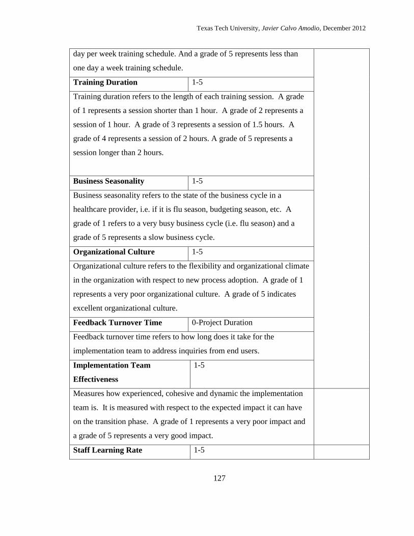
Texas Tech University, Javier Calvo Amodio, December 2012
127
day per week training schedule. And a grade of 5 represents less than
one day a week training schedule.
Training Duration 1-5
Training duration refers to the length of each training session. A grade
of 1 represents a session shorter than 1 hour. A grade of 2 represents a
session of 1 hour. A grade of 3 represents a session of 1.5 hours. A
grade of 4 represents a session of 2 hours. A grade of 5 represents a
session longer than 2 hours.
Business Seasonality 1-5
Business seasonality refers to the state of the business cycle in a
healthcare provider, i.e. if it is flu season, budgeting season, etc. A
grade of 1 refers to a very busy business cycle (i.e. flu season) and a
grade of 5 represents a slow business cycle.
Organizational Culture 1-5
Organizational culture refers to the flexibility and organizational climate
in the organization with respect to new process adoption. A grade of 1
represents a very poor organizational culture. A grade of 5 indicates
excellent organizational culture.
Feedback Turnover Time 0-Project Duration
Feedback turnover time refers to how long does it take for the
implementation team to address inquiries from end users.
Implementation Team
Effectiveness
1-5
Measures how experienced, cohesive and dynamic the implementation
team is. It is measured with respect to the expected impact it can have
on the transition phase. A grade of 1 represents a very poor impact and
a grade of 5 represents a very good impact.
Staff Learning Rate 1-5

Texas Tech University, Javier Calvo Amodio, December 2012
128
Staff learning rate refers to the overall learning ability of the staff. A
grade of 1 represents a very poor learning rates and a grade of 5
represents excellent learning rates.
Communication Skills 1-5
Communication skills refers to the organization’s personnel ability and
willingness to communicate with each other. A grade of 1 represents
very poor communication skills and a grade of 5 represents excellent
communication skills.
Staff Experience 1-5
Staff experience refers to the level of experience that the staff possesses
both in professional jobs and in a job related to their current one. A
grade of 1 indicates no experience and a grade of 5 indicates a lot of
relevant experience.
Staff Educational Level 1-5
Staff educational level refers to the minimum and maximum academic
levels achieved by the staff. A grade of 1 indicates incomplete K-12
education. A grade of 5 indicates graduate degrees.
Existence of SOPs 0 or 1
A grade of 0 represents no presence of SOPs. A grade of 1 represents
existence of SOPs.
Desired Percentage of errors per
day
0 to 100% calculated from number
of errors committed per day
divided by total number of
transactions.
Based on historical performance expectations before implementation

Texas Tech University, Javier Calvo Amodio, December 2012
129
Percentage of errors per day
throughout the project duration
0 to 100% calculated from number
of errors committed per day
divided by total number of
transactions.
Excel
spreadsheet
generated by
managers
from their
databases.
The data was filled using the control panel view of the model (Figure 6-1). The control
panel is built to ease the input of factors’ values and to allow the use of the SyntheSim
mode in Vensim. The SyntheSim mode allows managers to vary factor values, test
different policies and identify how they can best use their resources to reach the desired
goal I accordance to Figure 2-19.
Table 6-2 presents the values for all sub-structure factors for the clinic. All these factors
were provided by the clinic’s process change manager based on his knowledge of the
system. This data is of qualitative nature.
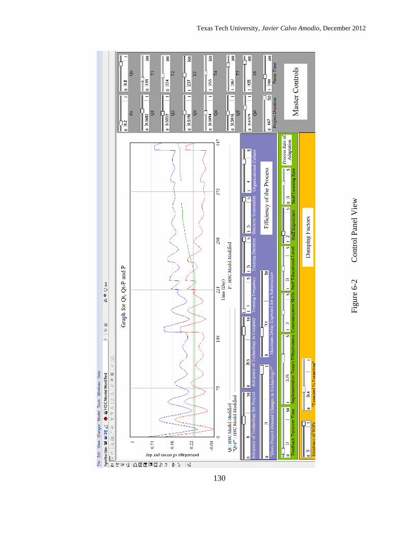
Texas Tech University, Javier Calvo Amodio, December 2012
130
Fig
ure
6-2
C
ontr
ol
Pan
el V
iew

Texas Tech University, Javier Calvo Amodio, December 2012
131
Table 6-2 Short-term lived project parmeters
Variable Output Value
Adequacy of Technology in Company 6
Adequacy of Technology for Project 8.5
Does Project Demand Changes in Technology? 1
Training Frequency 1
Training Duration 5
Business Seasonality 5
Organizational Culture 4
Feedback Turnover Time 3
Implementation Team Effectiveness 3.75
Staff Learning Rate 3
Communication Skills 3
Staff Experience 2
Staff Educational Level 3
Existence of SOPs 1
Expected % of Forgetting 40%
Desired Percentage of errors per day 20%
Long-term multi-phase project
The project is of a clerical section of an electronic health records implementation over a
healthcare center’s different clinics with different rollout times. The electronic health
records implementation focused on the clerical work related to billing processes. The
project was scheduled to last 440 days. Management expected the process to start with
80% errors per day; however data shows that 29.11% was the initial percentage of errors
per day. The initial “low” percentage of errors per day can be attributed to being rolled
out into only one clinic. However the percentage of errors per day increased as more
clinics were rolled out as shown in Table 6-3 and Figures 6-3 to 6-5. Qi represents the
initial percentage of errors per day per new phase and Ti the time counted in days after
the initial rollout.
Table 6-3 Multiple-Phase Factor Values
Q1= 57% Q2= 51% Q3= 52% Q4= 51% Q5= 50% Q6= 69%
T1= 159 T2= 224 T3= 237 T4= 265 T5= 387 T6= 435

Texas Tech University, Javier Calvo Amodio, December 2012
132
Figure 6-3 Historical Data Plot as Prcentage of Errors per Day
Figure 6-4 Model Generated Data Plot as Prcentage of Errors per Day

Texas Tech University, Javier Calvo Amodio, December 2012
133
Figure 6-5 Model Generated Data vs. Historical Data Plot as Percentage of Errors per
Day
Figure 6-6 Historical and Model Generated Data Variances Plot

Texas Tech University, Javier Calvo Amodio, December 2012
134
Conclusions
In Figure 6-5 it can be observed that the model does a good job at predicting the general
path of the historical data. The oscillation shown is also in accordance to the manager’s
accounts of the implementation process, meaning that there was much instability in the
implementation process. Figure 6-6 is presented to explain the differences observed in
Figure 6-5. As expected the model generated data presents more variation, due to the
intrinsic dampened oscillation, that indicates instability in the process. Figure 6-7 is a
histogram calculated over the differences between the model generated data and the
historical data; it shows that the model in a general sense does a decent job at tracking the
real world data, but there is an inevitable bias due to the dampened oscillation.
Therefore, a good measurement to assess whether the model identified periods of
instability and predicted the path would be to construct a histogram plot like Figure 6-7
and if the plot shows a similar shape, then it can be assumed that the model was accurate.
The R2 for the paired comparison of both data sets is 0.1149, indicating a low model
Figure 6-7 Histogram of Differences Between Historical and Model Generated Data Plot

Texas Tech University, Javier Calvo Amodio, December 2012
135
forecasting description capacity which confirms the observations presented in Figures 6-
4, 6-5 and 6-6. This means that under long term projects the model is not to be used to
forecast exact data patters. It should be used to identify periods of instability (where
oscillation exists), however the model is still capable to identify general trend of the
transition-phase.
From the results it can be inferred that the model is adequate to predict periods of
instability in the implementation process and the general path the real implementation
will follow. Further experimentation is required to validate this observation and is
discussed in chapter 8.
Future Work
Forecasting capabilities
Even though the results are encouraging, further experimentation to validate capabilities
of the model to predict within short, mid and long term projects is necessary to better
understand the capabilities of the model.
Further investigation on the meaning of the histogram and R2
Even though Figure 6-7 and the R2 values agree in the sense that the model does not do a
good job at forecasting individual data points, further research is necessary to establish
the exact relationship between these two tests and how to use them to have better
understanding of the model.
Detailed measurement methods
Develop quantitative methods to estimate initial percentage of errors per day. This
includes decrease in efficiency as a result of subsequent rollouts of new subsystems into
the transition-phase.
Texas Tech University, Javier Calvo Amodio, December 2012
136
Forecasting ability
Explore if higher resolution level and probably a dynamic behavior for the factors in each
of the substructures can enhance the forecasting ability of the model.
REFERENCES
Berwick, D., Kabcenell, A., & Nolan, T. (2005). No Toyota yet, but a start. A cadre of
providers seeks to transform an inefficient industry--before it's too late. Modern
healthcare, 35(5), 18.
Calvo-Amodio, J., Patterson, P.E., Smith, M.L., Burns, J. “A Generalized System
Dynamics Model for Managing Transition-Phases in Healthcare Environments”.
Target Journal: Systems Practice and Action Research.
de Souza, L.B. (2009). Trends and approaches in lean healthcare. Leadership in Health
Services, 22(2), 121-139.
Eden, C., & Huxham, C. (1996). Action research for management research. British
Journal of Management, 7(1), 75-86.
Rosmulder, RW, Krabbendam, JJ, Kerkhoff, A.H.M., Houser, CM, & Luitse, J.S.K.
(2011). Computer Simulation Within Action Research: A Promising Combination
for Improving Healthcare Delivery? Systemic practice and action research, 1-16.

Texas Tech University, Javier Calvo Amodio, December 2012
137
CHAPTER VII
7. APPLICATION OF TRANSITION-PHASE MANAGEMENT MODEL FOR AN
ELECTRONIC HEALTH RECORD SYSTEM IMPLEMENTATION
Abstract
The implementation of an electronic health records system requires changes in processes,
which in turn require management of such transition-phases. Electronic health records
systems implementations are composed of various subsystems such as medical, clerical,
administrative and billing. The complexity of each an electronic health records
implementation in each of these subsystems is affected by project length, and size
measured by the number of places it is deployed and the timing of each deployment. An
evaluation of the transition-phase management model on a short and a mid-term
electronic health records implementation process is presented. Analysis of the adequacy
and accuracy of the model is provided and guidelines for interpretation are suggested.
Introduction
The transition-phase management model, developed by Calvo-Amodio, et. al. (201X)
present a method to evaluating the capabilities of an organization to implement an
electronic health records system according to their current state and resources available.
In this paper, the transition-phase management model is evaluated against one short-term
and one mid-term electronic health records system implementation project.
Background
Complementary use of methodologies with lean thinking
Several attempts to combine methodologies, such as managerial philosophies like total
quality management, six sigma, theory of constraints, reengineering, and discrete event
simulation(de Souza, 2009, p. 125) to overcome their inherent limitations have been

Texas Tech University, Javier Calvo Amodio, December 2012
138
attempted, all arising from the authors' observations that single methodologies are rarely
a one-size-fits-all solution. Yasin et al (Yasin, Zimmerer, Miller, & Zimmerer, 2002)
conducted an investigation to evaluate the effectiveness of some managerial philosophies
applied into a healthcare environment. The authors report that "it is equally clear from
the data that some tools and techniques were more difficult to implement than others"
(Yasin et al., 2002, p. 274), implying that many of the failures were due to inadequate
implementations or lack of understanding of the scope. From a systems thinking
perspective, these two types of failures in implementing a methodology are explained by
the methodology's inability to deal with very specific problem situations. This supports
the point that a complementarist industrial engineering and engineering management -
systems thinking approach can be explored by taking an atypical approach by tackling
""small"" problems, instead of large and complex problems. This approach should
convince management of the effectiveness of a complementarist managerial philosophy
using systems thinking.
Lean Six Sigma
Consider the case of the Lean Six Sigma (LSS) philosophy as an example of a
methodology that was built to enhance its constituent methodologies strengths and further
their scope. On one end we have a six sigma focus on the "lowest hanging apples"
(Arnheiter & Maleyeff, 2005, p. 12), which may not be the best place to start. On the
other end, lean thinking focuses on waste reduction from the consumer perspective,
without consideration of quality or stability of processes. The complementarist Lean Six
Sigma approach suggests that Lean organizations can gain “a good balance between an
increase in value of the product (as viewed by the customer) and cost reduction in the
process [as] an outcome of combining Lean and SS” (Arnheiter & Maleyeff, 2005, p. 16).
The authors suggest that an organization that follows the Lean Six Sigma philosophy
would possess key characteristics belonging to both philosophies, as stated in Table 2-1
(Arnheiter & Maleyeff, 2005)

Texas Tech University, Javier Calvo Amodio, December 2012
139
Table 7-1 Organizational Lean Six Sigma Characteristics
Lean Six Sigma
(1) It would incorporate an overriding
philosophy that seeks to maximize the
value-added content of all operations.
(1) It would stress data-driven
methodologies in all decision making, so
that changes are based on scientific rather
than ad hoc studies.
(2) It would constantly evaluate all
incentive systems in place to ensure that
they result in global optimization instead of
local optimization.
(2) It would promote methodologies that
strive to minimize variation of quality
characteristics.
(3) It would incorporate a management
decision-making process that bases every
decision on its relative impact on the
customer.
(3) It would design and implement a
company-wide and highly structured
education and training regimen.
The authors also posit how a LSS approach would balance value and costs as perceived
by the customer and producer respectively (see Figure 2-2 (Arnheiter & Maleyeff, 2005,
p. 16).
Figure 7-1 Nature of competitive advantage.

Texas Tech University, Javier Calvo Amodio, December 2012
140
Socio-technical systems - lean thinking
Joosten, Bongers and Janssen (2009, p. 344) take a socio-technical systems approach to
lean thinking. They suggest that value in lean thinking “is not seen as an individual level
concept, but as a system property. According to lean, a system has an inherent, maximal
value that is bounded by its design, rather than by the will, experience or attitude of
individual members”. They state that socio-technical systems can provide a framework
to improve healthcare delivery by complementing the intrinsic operational approach of
lean thinking with the social aspect of implementations.
Knowledge Production as a Control Variable
Dorroh, Gulledge, and Womer (1994) state that at the beginning of a new process
implementation, education and training are the primary tasks performed by the worker,
and as the project advances then production becomes dominant (p. 947). Their model is
different from a learning-by-doing model because “knowledge is produced independent
of production experience” (p. 952). Dorroh, Gulledge, and Womer (1994) state that
higher levels of knowledge allow for easier knowledge production, resulting in more
resources allocated for learning, and a faster rate of knowledge production –or a sharper
learning curve. They conclude that knowledge creation is a managerial decision, and that
the rate of knowledge production is a control variable (p.957). As the process
implementation advances, the need to generate more knowledge (knowledge value)
decreases, reducing the resources devoted to knowledge generation (Dorroh et al., 1994,
p. 955; Epple, Argote, & Devadas, 1991, p. 65).
According to Epple, Argote, & Devadas (1991), learning from the experience of others
can benefit an organization. It is worth noting that knowledge acquired through learning
will depreciate at a relatively fast rate. Epple, Argote, & Devadas (1991) also state that
when learning caused by the use/implementation of new technologies, then learning will
transfer –at least partially from one department to another, from one shift to another as
long as that technology is used within.

Texas Tech University, Javier Calvo Amodio, December 2012
141
For further reference, read Yelle (1979) and Levy (1965) for reviews of the learning
curve literature.
Learning Loop Model
Sterman (Senge, 2006; 1994, 2000) introduced an idealized learning loop model (Figure
7-2 ).
Real World Unknown structure
Dynamic complexity
Time delays
Inability to conduct controlled experiments
Virtual World Known structure
Variable level of complexity
Controlled experiments
Virtual World
Implementation
failure
Game playing Inconsistency
Performance is goal
Real World Perfect
implementation
Consistent incentives
Consistent
application of decision rules
Learning can be goal
Decisions
Virtual World
Complete, accurate,
immediate
feedback
Real World
Selective perception
Missing feedback
Delay Bias, distortion,
error
Ambiguity
Information Feedback
Strategy, structure, and
decision rules
Simulation used to infer
dynamics of cognitive maps
correctly
Mental Models Mapping of feedback
structures
Disciplined application of
scientific reasoning
Discussability of group
process, defensive behavior.
Figure 7-2 Idealized learning loops.

Texas Tech University, Javier Calvo Amodio, December 2012
142
The validity of the model Sterman introduces is that it provides a good justification for
the use of simulation models as learning tools. By simplifying reality and putting it into a
virtual world, it is possible to perform experiments within it. Policies and approaches can
be challenged by managers without having to wait for feedback from reality, which can
be expensive.
Problem Context
In order to complete the model control validation (Figure 3-5) one more experiment is
required. In this experiment focus is placed on a short-lived and a mid-lived project.
Data about errors per day committed by end users of a new electronic health records
process was provided by a local healthcare clinic.
Oral in-person sessions were conducted resulting in agreement of the clinic to provide
qualitative and quantitative data regarding the implementation process. All identifiers
from personnel related data was removed by the data providers, eliminating the
possibility for the researchers to relate data to any staff member. The procedure for data
collection and a handout containing the major steps are presented below.
Data Collection Procedure
Data was obtained through interviews with the process change manager. Table 7-1
presents a summary of the data required:
Table 7-2 Summary of Data
Variable Output Value Delivery
Format
Adequacy of Technology in Company 1-10 Fill-in format
to be provided
to managers.
Refers to how well does the current technology (computing, software,
communications) contributes to their operations. A grade of 1
represents very poorly and a grade of 5 excellent.

Texas Tech University, Javier Calvo Amodio, December 2012
143
Adequacy of Technology for
Project
1-10
Refers to how well does the current technology (computing, software,
communications) is aligned with the process requirements of the new
process to be implemented. A grade of 1 represents very poorly and a
grade of 5 excellent.
Training Frequency 1-5
Training frequency refers to how close from each other are held the
training sessions. A grade of 1 represents a daily training schedule. A
grade of 2 represents a 3 day a week training schedule. A grade of 3
represents 2 days a week training schedule. A grade of 4 represents 1
day per week training schedule. And a grade of 5 represents less than
one day a week training schedule.
Training Duration 1-5
Training duration refers to the length of each training session. A grade
of 1 represents a session shorter than 1 hour. A grade of 2 represents a
session of 1 hour. A grade of 3 represents a session of 1.5 hours. A
grade of 4 represents a session of 2 hours. A grade of 5 represents a
session longer than 2 hours.
Business Seasonality 1-5
Business seasonality refers to the state of the business cycle in a
healthcare provider, i.e. if it is flu season, budgeting season, etc. A
grade of 1 refers to a very busy business cycle (i.e. flu season) and a
grade of 5 represents a slow business cycle.
Organizational Culture 1-5
Organizational culture refers to the flexibility and organizational climate
in the organization with respect to new process adoption. A grade of 1
represents a very poor organizational culture. A grade of 5 indicates

Texas Tech University, Javier Calvo Amodio, December 2012
144
excellent organizational culture.
Feedback Turnover Time 0-Project Duration
Feedback turnover time refers to how long does it take for the
implementation team to address inquiries from end users.
Implementation Team
Effectiveness
1-5
Measures how experienced, cohesive and dynamic the implementation
team is. It is measured with respect to the expected impact it can have
on the transition phase. A grade of 1 represents a very poor impact and
a grade of 5 represents a very good impact.
Staff Learning Rate 1-5
Staff learning rate refers to the overall learning ability of the staff. A
grade of 1 represents a very poor learning rates and a grade of 5
represents excellent learning rates.
Communication Skills 1-5
Communication skills refers to the organization’s personnel ability and
willingness to communicate with each other. A grade of 1 represents
very poor communication skills and a grade of 5 represents excellent
communication skills.
Staff Experience 1-5
Staff experience refers to the level of experience that the staff possesses
both in professional jobs and in a job related to their current one. A
grade of 1 indicates no experience and a grade of 5 indicates a lot of
relevant experience.
Staff Educational Level 1-5
Staff educational level refers to the minimum and maximum academic
levels achieved by the staff. A grade of 1 indicates incomplete K-12
education. A grade of 5 indicates graduate degrees.
Existence of SOPs 0 or 1

Texas Tech University, Javier Calvo Amodio, December 2012
145
A grade of 0 represents no presence of SOPs. A grade of 1 represents
existence of SOPs.
Desired Percentage of errors per
day
0 to 100% calculated from number
of errors committed per day
divided by total number of
transactions.
Based on historical performance expectations before implementation
Percentage of errors per day
throughout the project duration
0 to 100% calculated from number
of errors committed per day
divided by total number of
transactions.
Excel
spreadsheet
generated by
managers
from their
databases.
The data is to be filled using the control panel view of the model (Figure 7-1). The
control panel is built to ease the input of factors’ values and to allow the use of the
SyntheSim mode in Vensim. The SyntheSim mode allows managers to vary factor
values, test different policies and identify how they can best use their resources to reach
the desired goal I accordance to Figure 2-19.
Table 7-2 presents the values for all sub-structure factors for the clinic. All these factors
were provided by the clinic’s process change manager based on his knowledge of the
system. This data is of qualitative data.

Texas Tech University, Javier Calvo Amodio, December 2012
146
Fig
ure
7-3
C
ontr
ol
Pan
el V
iew

Texas Tech University, Javier Calvo Amodio, December 2012
147
Short-term project
The short-term project is of a clerical section of an electronic health records
implementation. The electronic health records implementation focused on patient
registration, billing information generation and check-out processes. The project was
scheduled to last 27 days. It was expected to and started with 20% errors per day as a
result of good training programs and the simplicity of the new process to be
implemented. Table 7-3 presents all the detailed factors values.
Table 7-3 Short-term lived project parmeters
Variable Output Value
Adequacy of Technology in Company 6
Adequacy of Technology for Project 9
Does Project Demand Changes in Technology? 1
Training Frequency 2
Training Duration 5
Business Seasonality 3
Organizational Culture 3.5
Feedback Turnover Time 3
Implementation Team Effectiveness 3.75
Staff Learning Rate 3.5
Communication Skills 3.75
Staff Experience 4
Staff Educational Level 3.25
Existence of SOPs 1
Expected % Forgetting 20%
Desired Percentage of errors per day 5%
Figures 7-4 to 7-8 present results and analyses on the model. After the Figures a detailed
analysis on their meaning is presented.

Texas Tech University, Javier Calvo Amodio, December 2012
148
Figure 7-4 Historical Data Plot as Prcentage of Errors per Day
Figure 7-5 Model Generated Data Plot as Prcentage of Errors per Day

Texas Tech University, Javier Calvo Amodio, December 2012
149
Figure 7-6 Model Generated Data vs. Historical Data Plot as Percentage of Errors per
Day
Figure 7-7 Historical and Model Generated Data Variances Plot

Texas Tech University, Javier Calvo Amodio, December 2012
150
Mid-Term Project
The mid-term project is of a clerical section of the medical processes from the same
healthcare clinic as in section 7.1. The electronic health records implementation focused
on patient hand in from check in to providers, flow throughout the different providers,
and hand in to check-out. The project was scheduled to last 97 days. It started with 56%
errors per day as a result of being rolled while the short-term project was being
concluded, situation that required training during another project rollout, and the
complexity of the new process to be implemented. Table 7-4 presents all the detailed
factors values and Figure 7-9 presents the control panel with the factor values.
Figure 7-8 Histogram of Differences Between Historical and Model Generated Data
Plot

Texas Tech University, Javier Calvo Amodio, December 2012
151
Table 7-4 Short-term lived project parmeters
Variable Output Value
Adequacy of Technology in Company 6
Adequacy of Technology for Project 9
Does Project Demand Changes in Technology? 1
Training Frequency 2
Training Duration 5
Business Seasonality 3
Organizational Culture 3.5
Feedback Turnover Time 3
Implementation Team Effectiveness 3.75
Staff Learning Rate 3.5
Communication Skills 3.75
Staff Experience 4
Staff Educational Level 3.25
Existence of SOPs 1
Expected % Forgetting 20%
Desired Percentage of errors per day 5%

Texas Tech University, Javier Calvo Amodio, December 2012
152
Fig
ure
7-9
C
ontr
ol
Pan
el V
iew
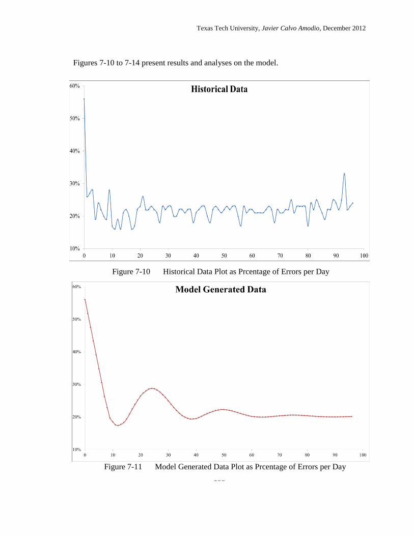
Texas Tech University, Javier Calvo Amodio, December 2012
153
Figures 7-10 to 7-14 present results and analyses on the model.
Figure 7-10 Historical Data Plot as Prcentage of Errors per Day
Figure 7-11 Model Generated Data Plot as Prcentage of Errors per Day

Texas Tech University, Javier Calvo Amodio, December 2012
154
Figure 7-12 Model Generated Data vs. Historical Data Plot as Percentage of Errors per
Day
Figure 7-13 Historical and Model Generated Data Variances Plot

Texas Tech University, Javier Calvo Amodio, December 2012
155
Conclusions
Short-term project
Figure 7-5 shows a very good fit for the model generated data against the historical data
in path, it looks like a fitted function. Figure 7-7 helps illustrate the last point in that the
histogram for the differences shows normality with little kurtosis and skewedness.
Figure 7-6 is used to explain the differences between the variances, and as expected the
real world data shows more variation than the model generated data; a characteristic that
helps explain the quasi fitted line behavior of the model generated data. The R2 for the
paired comparison of both data sets is 0.86, indicating a very good model forecasting
description capacity which confirms the observations presented in Figures 7-5, 7-6 and 7-
7.
Figure 7-14 Histogram of Differences Between Historical and Model Generated Data
Plot

Texas Tech University, Javier Calvo Amodio, December 2012
156
From the results it can be inferred that when the difference between the initial percentage
of errors per day and the desired percentage of errors per day, the length of the project is
short, and the values of all factors are set around a moderate scenario, the model is
capable to indicate the path that the implementation percentage of errors per day will
follow. Further experimentation is required to validate this observation and is discussed
in the final section of this paper.
Mid-term project
Figure 7-12 shows a good fit for the model generated data against the historical data in
path, and portrays dampened oscillation in a phase of the implementation that the
manager identified as an adjustment phase. Figure 7-13 is used to explain the differences
between the variances, and as expected the real world data shows more variation than the
model generated data. Figure 7-14 helps illustrate the goodness of fit of the model
generated data versus the historical data. The histogram for the differences shows
normality with some kurtosis and skewedness. The long left tail can be explained by the
warm-up period (dampened oscillation phase) in the model. The R2 for the paired
comparison of both data sets is 0.08384, indicating a poor model forecasting description
capacity which confirms the observations presented in Figures 7-12, 7-13 and 7-14.
What the histogram and R2 value mean is that even though the model is capable of
providing a good representation of the path, the actual fit when a point-to-point pairwise
comparison is performed is poor, meaning that the model is not good to forecasting data.
From the results it can be inferred that at mid length projects with medium difference
between the initial and desired percentage of errors per day the model is capable of
indicating the path that the real world implementation will follow in addition to
identifying periods of instability. Further experimentation is required to validate this
observation and is discussed in chapter 8.

Texas Tech University, Javier Calvo Amodio, December 2012
157
Future research
Dynamic equilibrium determination
It is important to be able to determine when periods of instability and stability (dynamic
equilibrium) will occur within a new process implementation to better anticipate them.
For that end, a proposed methodology was identified during the development of this
dissertation, however it still need more development.
Further investigation on the meaning of the histogram and R2
Even though Figures 7-7 and 7-14 and the R2 values agree in the sense how the model
forecasts individual data points, further research is necessary to establish the exact
relationship between these two tests and how to use them to have better understanding of
the model.
Dynamic equilibrium
The suggested tool for managers to evaluate when they can expect that the period of
instability will be over can be done as follows and shown in Figure 7-14. A manager
may determine that a 5% variation would be acceptable, and then by measuring the
Euclidean distance from the top of consecutive hills of the model generated data the
manager can determine where the model becomes stable.
Therefore, determination of what can be constituted as an acceptable variation, and a
mathematical generalizable procedure to determine points of inflection between
instability and stability (dynamic equilibrium) need to be developed.

Texas Tech University, Javier Calvo Amodio, December 2012
158
Figure 7-15 Instability Period End Concept for Proposed Test
0.2727%
0.0170%
0.06470%

Texas Tech University, Javier Calvo Amodio, December 2012
159
REFERENCES
Arnheiter, E.D., & Maleyeff, J. (2005). The integration of lean management and Six
Sigma. The TQM magazine, 17(1), 5-18.
Calvo-Amodio, J., Patterson, P.E., Smith, M.L., Burns, J. “A Generalized System
Dynamics Model for Managing Transition-Phases in Healthcare Environments”.
Target Journal: Systems Practice and Action Research.
de Souza, L.B. (2009). Trends and approaches in lean healthcare. Leadership in Health
Services, 22(2), 121-139.
Dorroh, J.R., Gulledge, T.R., & Womer, N.K. (1994). Investment in knowledge: A
generalization of learning by experience. Management Science, 947-958.
Epple, D., Argote, L., & Devadas, R. (1991). Organizational learning curves: A method
for investigating intra-plant transfer of knowledge acquired through learning by
doing. Organization Science, 58-70.
Joosten, T., Bongers, I., & Janssen, R. (2009). Application of lean thinking to health care:
issues and observations. International Journal for Quality in Health Care, 21(5),
341.
Levy, F.K. (1965). Adaptation in the production process. Management Science, 136-154.
Senge, PM. (2006). The fifth discipline: The art and practice of the learning organization:
Currency.
Sterman, JD. (1994). Learning in and about complex systems. System Dynamics Review,
10(2-3), 291-330.
Sterman, JD. (2000). Business dynamics: Systems thinking and modeling for a complex
world with CD-ROM: Irwin/McGraw-Hill.
Yasin, M.M., Zimmerer, L.W., Miller, P., & Zimmerer, T.W. (2002). An empirical
investigation of the effectiveness of contemporary managerial philosophies in a
hospital operational setting. International Journal of Health Care Quality
Assurance, 15(6), 268-276.
Yelle, L.E. (1979). The learning curve: Historical review and comprehensive survey.
Decision Sciences, 10(2), 302-328.

Texas Tech University, Javier Calvo Amodio, December 2012
160
CHAPTER VIII
8. CONCLUSION
Features of this Research
The model is developed to help healthcare managers manage transition-phases in their
organizations. Managers can determine their objective function in accordance to Figure
8-1
Figure 8-1 can be used as follows:
1. If managers choose to maximize the quality of the new process implementation
(minimize the difference between the current state and the desired state), the
model will help them to find the best balance between resources costs and
completion time.
Figure 8-1 Objective Function for Transition Phase Management Model
(Figure 2-19)
Quality
min Qt−P
Time
min tf−t0
Cost
min F−a−µ
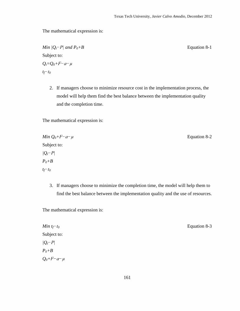
Texas Tech University, Javier Calvo Amodio, December 2012
161
The mathematical expression is:
Min |Qt−P| and P0+B Equation 8-1
Subject to:
Qt=Q0+ − −µ
tf− 0
2. If managers choose to minimize resource cost in the implementation process, the
model will help them find the best balance between the implementation quality
and the completion time.
The mathematical expression is:
Min Q0+ − −µ Equation 8-2
Subject to:
|Qt−P|
P0+B
tf− 0
3. If managers choose to minimize the completion time, the model will help them to
find the best balance between the implementation quality and the use of resources.
The mathematical expression is:
Min tf− 0 Equation 8-3
Subject to:
|Qt−P|
P0+B
Q0+ − −µ

Texas Tech University, Javier Calvo Amodio, December 2012
162
By using repeatedly the model, managers will learn about their organization (see section
8.3 for details). Under repeated use, a double loop learning process as portrayed in
Figure 2-4 is generated.
As it has been presented in chapters VI and VII, the model requires little (chapter VI) to
no modification (Chapter VII) and presents the managers a user friendly interface
(Figures 6-1, 7-1 and 7-7) to input all parameters. The model can be used with any
version of Vensim simulation software under its SyntheSim function thus minimizing the
need to invest in expensiv e versions of the software.
Findings from this Research
Complementarist Approach:
It is possible to develop an accurate simulation model based on a complementarist
approach using Levy’s (1965) adaptation function, systemic concepts (system archetypes)
and System Dynamics theory.
Validity of the model:
As presented in section 2.3 and chapters IV and V the model is capable of reproducing
the behaviors of the balancing loop, drifting goals and unintended consequences system
archetypes though an exponential decay (or growth depending on the parameters) and
with dampened oscillation as the process gains stability.
Dynamic Hypotheses
Chapters VI and VI presented that the model is capable to reproduce the behavior over-
time presented in Dynamic Hypothesis (Figures 6-2, 7-2 and 7-8). The model will
indicate the path of the dynamic hypothesis, and indicate periods of instability.

Texas Tech University, Javier Calvo Amodio, December 2012
163
Research applicability
Healthcare managers will benefit from the se of the model in the following ways:
1. First time use: the model will provide managers an assessment of their
organization’s capabilities to implement new processes. They can identify their
areas of opportunity and evaluate which area can have the biggest impact to
achieve the desired outcome.
2. Repeated use: will provide organizational learning (double-loop learning
approach) by allowing the managers to further calibrate the model and their
organizations to function to the best of its possibilities.
Future Research Needs
Based on the papers presented in chapters V, VI and VII the transition-phase
management model can be enriched if the following areas are further explored:
Detailed measurement methods
Develop quantitative measurement methods to determine the sub-structure factors
values following a Bayesian approach.
Double loop learning process should be implemented to increase knowledge of
each variable within a same organization.
These points will enable the validation of the substructure values and variables used
along with the resolution level employed in the model.
Further investigation on the meaning of the histogram and R2
Both tools can be integrated to develop a statistical test for the managers to use in order
to assess the efficiency of their estimations of the parameters and to better calibrate their
assessments of their organizations versus the real world.

Texas Tech University, Javier Calvo Amodio, December 2012
164
Forecasting capabilities
Even though the results are encouraging, further experimentation to validate capabilities
of the model to predict within short, mid and long term projects is necessary to better
understand the capabilities of the model.
Training duration and frequency
Develop a quantitative measurement technique to determine the impact of the interaction
between training frequency and training duration. Throughout the model development it
was hypothesized that an optimum range for the interaction should exist. Figure 8-2
presents the conceptualized range.
Parameter optimization
Internal control parameters and weights were determined based on goal programming,
however there is still potential to optimize these parameters.
Therefore, the development of a state-space mathematical model can aid to proof
1 2 3 4 5
Training Frequency
Traini
ng
Durati
on
1
2
3
Hypothesized
Optimal
Range
Figure 8-2 Hypothesized Optimal Range Graph

Texas Tech University, Javier Calvo Amodio, December 2012
165
the concept and to determine accurate parameters.
In addition, the parameter optimization function in Vensim Professional should be
used to cross reference the findings from the state-space optimization.

Texas Tech University, Javier Calvo Amodio, December 2012
166
9. REFERENCES
Ackoff, R.L. (1973). Science in the systems age: beyond IE, OR, and MS. Operations
Research, 21(3), 661-671.
Adler, K.G. (2007). How to successfully navigate your EHR implementation. Family
practice management, 14(2), 33.
Adler, P.S., & Clark, K.B. (1991). Behind the learning curve: A sketch of the learning
process. Management Science, 267-281.
Argote, L., & Epple, D. (1990). Learning curves in manufacturing. Science, 247(4945),
920.
Arnheiter, E.D., & Maleyeff, J. (2005). The integration of lean management and Six
Sigma. The TQM magazine, 17(1), 5-18.
Barlas, Y. (1996). Formal aspects of model validity and validation in system dynamics.
System dynamics review, 12(3), 183-210.
Bellinger, G. (2004). Archetypes: Interaction Structures of the Universe. Retrieved
1/18/2012, 2012, from http://www.systems-thinking.org/arch/arch.htm
Benneyan, J.C. (1996). Using statistical process control (SPC) to measure and improve
health care quality.
Benneyan, J.C. (1998a). Statistical quality control methods in infection control and
hospital epidemiology, part I: Introduction and basic theory. Infection Control and
Hospital Epidemiology, 194-214.
Benneyan, J.C. (1998b). Statistical quality control methods in infection control and
hospital epidemiology, Part II: chart use, statistical properties, and research issues.
Infection Control and Hospital Epidemiology, 265-283.
Benneyan, J.C. (2001). Number-between g-type statistical quality control charts for
monitoring adverse events. Health Care Management Science, 4(4), 305-318.
Berwick, D., Kabcenell, A., & Nolan, T. (2005). No Toyota yet, but a start. A cadre of
providers seeks to transform an inefficient industry--before it's too late. Modern
healthcare, 35(5), 18.
Callender, C., & Grasman, S.E. (2010). Barriers and Best Practices for Material
Management in the Healthcare Sector. Engineering Management Journal; EMJ,
22(4), 11.
Calvo-Amodio, J., Tercero, V.G., Hernandez-Luna, A.A., & Beruvides, M.G. (2011).
Applied Systems Thinking and Six Sigma: A Total Systems Intervention Approach.
Paper presented at the 2011 American Society for Engineering Management
International Annual Conference, Lubbock, Texas.
Carrillo, J.E., & Gaimon, C. (2000). Improving manufacturing performance through
process change and knowledge creation. Management Science, 265-288.
Checkland, P. (1979a). Techniques in Soft Systems Practice Part 1. Systems Diagrams
Some Tentative Guidelines. Journal of Applied Systems Analysis, 6, 33-40.
Checkland, P. (1979b). Techniques in soft systems practice, part 2: Building conceptual
models. Journal of Applied Systems Analysis, 6(4), 1-49.
Checkland, P. (1981). Systems thinking, systems practice: Wiley Chichester.

Texas Tech University, Javier Calvo Amodio, December 2012
167
Checkland, P. (1985). From optimizing to learning: A development of systems thinking
for the 1990s. Journal of the Operational Research Society, 757-767.
Checkland, P. (1988). The case for Holon. Systemic Practice and Action Research, 1(3),
235-238.
Checkland, P. (1999). Systems Thinking, Systems Practice. New York: Wiley.
Checkland, P. (2000). Soft systems methodology: a thirty year retrospective. Systems
Research.
Checkland, P, Forbes, P, & Martin, S. (1990). Techniques in soft systems practice. III,
Monitoring and control in conceptual models and in evaluation studies. Journal of
Applied Systems Analysis, 17, 29-37.
Checkland, P, & Scholes, J. (1990). Soft systems methodology in action: John Wiley &
Sons, Inc. New York, NY, USA.
de Souza, L.B. (2009). Trends and approaches in lean healthcare. Leadership in Health
Services, 22(2), 121-139.
Deming, WE. (1998). A system of profound knowledge. The Economic Impact of
Knowledge, 161.
Dorroh, J.R., Gulledge, T.R., & Womer, N.K. (1994). Investment in knowledge: A
generalization of learning by experience. Management Science, 947-958.
Eden, C., & Huxham, C. (1996). Action research for management research. British
Journal of Management, 7(1), 75-86.
Epple, D., Argote, L., & Devadas, R. (1991). Organizational learning curves: A method
for investigating intra-plant transfer of knowledge acquired through learning by
doing. Organization Science, 58-70.
Flood, R.L. (2010). The relationship of ‘systems thinking’to action research. Systemic
Practice and Action Research, 23(4), 269-284.
Flood, R.L., & Jackson, M.C. (1991). Creative problem solving: Wiley Chichester.
Forrester, J.W. (1961). Industrial Dynamics. New York: Productivity Press.
Forrester, J.W. (1971a). Counterintuitive behavior of social systems. Theory and
Decision, 2(2), 109-140.
Forrester, J.W. (1971b). World dynamics: Wright-Allen Press Cambridge, MA.
Forrester, J.W. (1980). Information sources for modeling the national economy. Journal
of the American Statistical Association, 75(371), 555-566.
Forrester, J.W. (1987a). Lessons from system dynamics modeling. System Dynamics
Review, 3(2), 136-149.
Forrester, J.W. (1987b). Nonlinearity in high-order models of social systems. European
Journal of Operational Research, 30(2), 104-109.
Forrester, J.W. (1991). System dynamics and the lessons of 35 years. The systemic basis
of policy making in the 1990s, 29, 4224-4224.
Forrester, J.W. (1992). Policies, decisions and information sources for modeling.
European Journal of Operational Research, 59(1), 42-63.
Forrester, J.W. (1994). System dynamics, systems thinking, and soft OR. System
Dynamics Review, 10(2 3), 245-256.
Forrester, J.W. (1995). The beginning of system dynamics. The McKinsey Quarterly(4),
4-5.

Texas Tech University, Javier Calvo Amodio, December 2012
168
Forrester, J.W. (1999). System Dynamics: the Foundation Under Systems Thinking.
Retrieved October, 13, 2002.
Forrester, J.W., & Senge, P.M. (1978). Tests for building confidence in system dynamics
models: System Dynamics Group, Sloan School of Management, Massachusetts
Institute of Technology.
Forrester, JW, Low, GW, & Mass, NJ. (1974). The debate on world dynamics: a response
to Nordhaus. Policy Sciences, 5(2), 169-190.
Forrester, JW, & Senge, PM. (1980). Tests for building confidence in system dynamics
models. TIMS studies in the management sciences, 14, 209-228.
Hannon, B.M., & Ruth, M. (2001). Dynamic modeling: Springer Verlag.
Homer, J., & Oliva, R. (2001). Maps and models in system dynamics: a response to
Coyle. System Dynamics Review, 17(4), 347-355.
Homer, J.B., & Hirsch, G.B. (2006). System dynamics modeling for public health:
background and opportunities. American Journal of Public Health, AJPH.
2005.062059 v062051.
Jackson, M.C. (1990). Beyond a system of systems methodologies. Journal of the
Operational Research Society, 657-668.
Jackson, M.C. (1991). Systems methodology for the management sciences: Plenum
Publishing Corporation.
Jackson, M.C. (2000). Systems Approaches to Management. New York: Kluwer
Academic/ Plenum Publishers.
Jackson, M.C. (2003). Systems thinking: Creative holism for managers: Wiley
Chichester.
Jackson, M.C., & Keys, P. (1984). Towards a system of systems methodologies. Journal
of the Operational Research Society, 473-486.
Joosten, T., Bongers, I., & Janssen, R. (2009). Application of lean thinking to health care:
issues and observations. International Journal for Quality in Health Care, 21(5),
341.
Lapré, M.A., Mukherjee, A.S., & Van Wassenhove, L.N. (2000). Behind the learning
curve: Linking learning activities to waste reduction. Management Science, 597-
611.
Laursen, M.L., Gertsen, F., & Johansen, J. (2003). Applying Lean Thinking in Hospitals-
Exploring Implementation Difficulties.
Levy, F.K. (1965). Adaptation in the production process. Management Science, 136-154.
Lewis, CI. (1924). Mind and the world-order: Dover Publications.
Lo, H.G., Newmark, L.P., Yoon, C., Volk, L.A., Carlson, V.L., Kittler, A.F., . . . Bates,
D.W. (2007). Electronic health records in specialty care: a time-motion study.
Journal of the American Medical Informatics Association, 14(5), 609-615.
Lundberg, R.H. (1956). Learning Curve Theory as Applied to Production Costs. SAE
Journal, 64(6), 48-49.
McGowan, J.J., Cusack, C.M., & Poon, E.G. (2008). Formative evaluation: a critical
component in EHR implementation. Journal of the American Medical Informatics
Association, 15(3), 297.
Midgley, G. (1990). Creative methodology design. Systemist, 12(3), 108-113.

Texas Tech University, Javier Calvo Amodio, December 2012
169
Midgley, G. (1997). Developing the methodology of TSI: From the oblique use of
methods to creative design. Systemic Practice and Action Research, 10(3), 305-
319.
Miller, R.H., & Sim, I. (2004). Physicians’ use of electronic medical records: barriers and
solutions. Health Affairs, 23(2), 116-126.
Morecroft, J.D.W., & Sterman, J. (2000). Modeling for learning organizations:
Productivity Pr.
Morrison, J.B. (2008). Putting the learning curve in context. Journal of Business
Research, 61(11), 1182-1190.
Newnan, D.G., Eschenbach, T., & Lavelle, J.P. (2004). Engineering economic analysis:
Oxford Univ Pr.
Pizziferri, L., Kittler, A.F., Volk, L.A., Shulman, L.N., Kessler, J., Carlson, G., . . . Bates,
D.W. (2005). Impact of an Electronic Health Record on oncol s s’ l .
Rosmulder, RW, Krabbendam, JJ, Kerkhoff, A.H.M., Houser, CM, & Luitse, J.S.K.
(2011). Computer Simulation Within Action Research: A Promising Combination
for Improving Healthcare Delivery? Systemic practice and action research, 1-16.
Senge, PM. (2006). The fifth discipline: The art and practice of the learning
organization: Currency.
Sterman, JD. (1994). Learning in and about complex systems. System Dynamics Review,
10(2-3), 291-330.
Sterman, JD. (2000). Business dynamics: Systems thinking and modeling for a complex
world with CD-ROM: Irwin/McGraw-Hill.
Sterman, JD. (2002). All models are wrong: reflections on becoming a systems scientist.
System Dynamics Review, 18(4), 501-531.
Taylor, F.W. (1911). The Principles of Scientific Management. New York: Harper &
Bros.
Terry, A.L., Thorpe, C.F., Giles, G., Brown, J.B., Harris, S.B., Reid, G.J., . . . Stewart, M.
(2008). Implementing electronic health records. Canadian Family Physician,
54(5), 730-736.
Towill, DR, & Christopher, M. (2005). An evolutionary approach to the architecture of
effective healthcare delivery systems. Journal of Health, Organisation and
Management, 19(2), 130-147.
von Bertalanffy, L. (1968). General Systems Theory. Harmondsworth: Pneguin.
Webmaster. (2012). Health Information and Management Systems. Retrieved 1/3/2012,
2012, from http://www.himss.org/ASP/topics_ehr.asp
Wilby, J. (1997). The observer's role and the process of critical review. Systemic Practice
and Action Research, 10(4), 409-419.
Wright-Patterson, TP. (1936). Factors Affecting the Cost of Airplanes. Journal of
Aeronautical Sciences, 3(4), 122-128.
Wyer, R. (1953). Learning curve helps figure profits, control costs. National Association
of Cost Accountants Bulletin, 35 (4), 490, 502.
Yasin, M.M., Zimmerer, L.W., Miller, P., & Zimmerer, T.W. (2002). An empirical
investigation of the effectiveness of contemporary managerial philosophies in a

Texas Tech University, Javier Calvo Amodio, December 2012
170
hospital operational setting. International Journal of Health Care Quality
Assurance, 15(6), 268-276.
Yelle, L.E. (1979). The learning curve: Historical review and comprehensive survey.
Decision Sciences, 10(2), 302-328.
Yoon-Flannery, K., Zandieh, S.O., Kuperman, G.J., Langsam, D.J., Hyman, D., &
Kaushal, R. (2008). A qualitative analysis of an electronic health record (EHR)
implementation in an academic ambulatory setting. Informatics in primary care,
16(4), 277-284.
Young, T. (2005). An agenda for healthcare and information simulation. Health Care
Management Science, 8(3), 189-196.
Zandieh, S.O., Yoon-Flannery, K., Kuperman, G.J., Langsam, D.J., Hyman, D., &
Kaushal, R. (2008). Challenges to EHR implementation in electronic-versus
paper-based office practices. Journal of general internal medicine, 23(6), 755-
761.

Texas Tech University, Javier Calvo Amodio, December 2012
171
10. APPENDIX A
INTERNAL REVIEW BOARD PROPOSAL
EXEMPT PROPOSAL FORMAT
FOR RESEARCH USING HUMAN SUBJECTS
Title: A Generalized System Dynamics Model for Managing Transition Phases in
Healthcare Environment
PI: Patrick E. Patterson, Ph.D., P.E., CPE
Co-PI: Milton L. Smith, Ph.D., P.E.
Co-PI: Javier Calvo Amodio
I. Rationale:
Combining industrial engineering and engineering management tools to improve a particular
problem situation in the healthcare industry has proven successful. The use of industrial
engineering and engineering management tools (scientific management approach) to improve
operation conditions and maximize revenue has been gaining popularity in the health care
environment. Examples range from the implementation of the TQM model, to the incorporation
of Lean thinking and Six Sigma methodologies.
The use of statistical process control (SPC), total quality management (TQM), six sigma,
lean thinking, and simulation as the main industrial engineering and engineering management
tools and philosophies in healthcare has been reported. The literature presents success cases,
reflects on failures, and suggests improvements in implementations of these methods and
philosophies in healthcare. For instance, Benneyan (1996) offers an overview of the possible
benefits that SPC could bring to healthcare. Warns about mistakes –such as using the wrong
charts and using shortcut formulas –that can be committed if SPC tools and their application are

Texas Tech University, Javier Calvo Amodio, December 2012
172
not understood correctly. Benneyan (1998a, 1998b, 2001) talks about control charts and their
potential uses in medical environment; also provides useful theoretical guidelines on how to
implement them, and analyzes their accuracy.
Callender and Grasman (2010) identify the following barriers to implementation of
supply chain management: Executive Support, Conflicting Goals, Skills and Knowledge,
Constantly Evolving Technology, Physician Preference, Lack of Standardized Codes, and
Limited Information Sharing. It is possible to extrapolate their reasoning to lean thinking
implementation, as they are new or foreign "IE tools" for the medical community considering
that acceptance of new ways is always a challenge.
Towill and Christopher (2005) advocate for the analog use of industrial logistics and
supply chain management in the National Health Service (NHS) in the United Kingdom. They
argue that material flow and pipeline concepts should be applied to the healthcare delivery
context to better match demand and the need for a more cost-effective practice.
Young (2005) proposes simulation as a tool to re-structure healthcare delivery on a
macro-level by researching patient flow, as the big hospitals go against Lean thinking principles
by promoting big queues. Young also suggests that system dynamics and theory of constraints
could work together since system dynamics is well suited to identify bottlenecks in a process (p.
192).
However, research of transition phases in a healthcare environment, using a holistic
scientific management approach, has received little attention. The estimation of time and
resources required to conduct a transition phase, usually employs “rule of thumb” approaches
based on simple calculations– rather than a holistic scientific management method. The
management of these transition phases has yet to be explored under a holistic scientific
management perspective. A transition phase management methodology will allow managers to
make better use of their resources, and to identify potential problems before they become too
costly.

Texas Tech University, Javier Calvo Amodio, December 2012
173
The study of the proposed methodology based on real world data is a requisite for
validation. Health Sciences Center and Community Health Center of Lubbock have accepted to
provide the necessary data of past projects to measure percentage of errors per day.
Relevant Definitions:
Problem Context
A situation where operational change is expected, requiring the implementation of a new process
or processes that entail staff training and learning by doing. When their efficiency is measured as
percentage of errors per day, healthcare managers are decision makers, and the healthcare
institution is subject to locally available resources such as staff, money, and training.
Generalized Model
A Generalized Model is a model that is commensurate with projects that align with the problem
context as defined for which requiring minimal or no adjustments necessary.
Transition-Phase Management
Transition-phase management is an operational change that is focused on minimizing the
percentage of errors per day, seen as learning by doing process. It is the result of the
implementation of projects that require changes in processes, and at times, of organizational
cultures
II. Subjects: Data about errors per day committed by end users or a new process are the
subjects; however there is no need to have any contact with these subjects. The subjects
involved directly are the managers in charge of implementing new processes at the Community
Health Center of Lubbock and the Health Sciences Center. Hereinafter the managers from
Health Sciences Center and Community Health Center of Lubbock are known as the data
providers.
The initial contact has already been established to determine the feasibility of the research. Oral
in-person recruitment sessions have been conducted resulting in agreement of both parties to
provide qualitative and quantitative data regarding the implementation process and staff
performance. All identifiers from personnel related data will be removed by the data providers,
eliminating the possibility for the researchers to relate data to any staff member. The procedure

Texas Tech University, Javier Calvo Amodio, December 2012
174
for data collection (see section III and appendices A and B for details) has been explained, and a
handout containing the major steps has been provided (see appendices A and B for details).
III. Procedures:
Academic Procedure
The variable of interest is percentage of errors per day (Qt) committed by staff throughout the
transition-phase management process. Model validation is conducted via the comparison of the
output from the model and the output of the real process. The output of the real process will be
expressed as behavior over time of the percentage of errors per day. For that, quantitative and
qualitative data regarding the variables presented in the following model are required:
Min: Equation 1 Transition-Phase Management
Subject to
where
Qt = percentage of errors per day
a = initial efficiency of the process = f(organizational culture, training. time)
µ = process rate of adaptation= f(experience, learning ability, feedback, time)
{ | |
| |
This includes obtaining historical information about employee performance such as errors
committed per day during new process implementation projects, frequency and duration of
training sessions, learning abilities (estimated by past performance of individuals), experience
measured in years in current position and in work force, and institutional feedback structures.

Texas Tech University, Javier Calvo Amodio, December 2012
175
The type of data to be collected can be quantitative and qualitative, depending on the data
availability and managerial practices of each data provider, and is related but not limited to years
of experience, number of training hours for a particular task, and learning ability (all descriptors
of errors committed). All data will be obtained only through the data providers, no interviews or
direct contact with employees is required.
To better illustrate the rationale of the procedure refer to Figure 1 that depicts the process
followed to build a system dynamics model. Note that quantitative and qualitative data are
important.
The data gathering process in a system dynamics model is iterative in nature. It starts with the
formulation of a dynamic hypothesis –or a theoretical model (see Figure 2). In it, the most basic
structure and data required are identified to generate the variable of interest: percentage errors
Policies, expectations and
structure,
Cause-to-effect direction
between variables
Concepts and abstractions,
Characteristics of learning
abilities, training sessions, etc.
Mental Data Base
Observation Experience
Written
Data Base
Numerical
Data Base
Figure 1. Mental Data Base and Decreasing Content of Written and
Numerical Data Bases (J. W. Forrester, 1980, p. 556)

Texas Tech University, Javier Calvo Amodio, December 2012
176
P
|Q(t)-P|
a
Q(t)+ -
+
+
F+
-
B
-
µ
++
+
Po
per day or Q(t). Only after the actual model is build and simulation starts is when more detail in
structure and data is slowly incorporated into the model until a reasonable degree of confidence
is reached (J. W. Forrester, 1971a, 1980, 1992; J. W. Forrester & Senge, 1978; J. Forrester &
Senge, 1980; Sterman, 2000, 2002). Figure 3 shows this process:
Equation 1 translates into the causal loop diagram shown in Figure 2.
A model building procedure requires three steps: identifying the system, simulating the system,
and controlling the system. Each step requires the use of three tools: creativity, choice, and
implementation. Creativity allows joining the researcher and manager’s mental data bases to
create dynamic structures by combining the written databases contained in the relevant literature.
Then a suitable structure is selected, and numerical databases are implemented into the system.
Table 1 indicates the goal for each one of the steps.
Figure 3. Model Validation Process
Figure 2 Initial Transition-Phase Management Model
SystemIdentification
Control Simulation
Creativity
Choice
Implementation
Creativity.
Creativity .
Implementation.Implementation .
Choice.
Choice .

Texas Tech University, Javier Calvo Amodio, December 2012
177
Table 1 Model Validation Matrix
Characteristic
Verification
First run
order Input Model Output
System
Identification 1 Known Unknown Known
Simulation 2 Known Known Unknown
Control 3 Unknown Known Known
Data and information obtained from the data providers will be used to validate the model in
accordance to Table 1.
Required Information:
Table 2 presents a list of the information that will be asked to Health Sciences Center and
Community Health Center of Lubbock managers.

Texas Tech University, Javier Calvo Amodio, December 2012
178
Table 2
Variable Output Value Delivery
Format
Adequacy of Technology in Company 1-5
Fill in format to
be provided to
Health Sciences
Center and
Community
Health Center of
Lubbock
managers.
Managers will be asked to make an assessment of how well does the current technology (computing,
software, communications) contributes to their operations. A grade of 1 represents very poorly and a
grade of 5 excellent.
Adequacy of Technology for Project 1-5
Managers will be asked to make an assessment of how well does the current technology (computing,
software, communications) is aligned with the process requirements of the new process to be
implemented. A grade of 1 represents very poorly and a grade of 5 excellent.
Training Frequency 1-5
Training frequency refers to how close from each other are held the training sessions. A grade of 1
represents a daily training schedule. A grade of 2 represents a 3 day a week training schedule. A
grade of 3 represents 2 days a week training schedule. A grade of 4 represents 1 day per week
training schedule. And a grade of 5 represents less than one day a week training schedule.
Training Duration 1-5
Training duration refers to the length of each training session. A grade of 1 represents a session
shorter than 1 hour. A grade of 2 represents a session of 1 hour. A grade of 3 represents a session of
1.5 hours. A grade of 4 represents a session of 2 hours. A grade of 5 represents a session longer than
2 hours.
Business Seasonality 1-5

Texas Tech University, Javier Calvo Amodio, December 2012
179
Business seasonality refers to the state of the business cycle in a healthcare provider, i.e. if it is flu
season, budgeting season, etc. A grade of 1 refers to a very busy business cycle (i.e. flu season) and a
grade of 5 represents a slow business cycle.
Organizational Culture 1-5
Organizational culture refers to the flexibility and organizational climate in the organization with
respect to new process adoption. A grade of 1 represents a very poor organizational culture. A grade
of 5 indicates excellent organizational culture.
Feedback Turnover Time 0-Project Duration
Feedback turnover time refers to how long does it take for the implementation team to address
inquiries from end users.
Implementation Team Effectiveness 1-5
Measures how experienced, cohesive and dynamic the implementation team is. It is measured with
respect to the expected impact it can have on the transition phase. A grade of 1 represents a very
poor impact and a grade of 5 represents a very good impact.
Staff Learning Rate 1-5
Staff learning rate refers to the overall learning ability of the staff. A grade of 1 represents a very
poor learning rates and a grade of 5 represents excellent learning rates.

Texas Tech University, Javier Calvo Amodio, December 2012
180
Table 2 (Continued)
Variable Output Value Delivery
Format
Communication Skills 1-5
Communication skills refers to the organization’s personnel ability and willingness to communicate
with each other. A grade of 1 represents very poor communication skills and a grade of 5 represents
excellent communication skills.
Staff Experience 1-5
Staff experience refers to the level of experience that the staff possesses both in professional jobs and
in a job related to their current one. A grade of 1 indicates no experience and a grade of 5 indicates a
lot of relevant experience.
Staff Educational Level 1-5
Staff educational level refers to the minimum and maximum academic levels achieved by the staff. A
grade of 1 indicates incomplete K-12 education. A grade of 5 indicates graduate degrees.
Existence of SOPs 0 or 1
A grade of 0 represents no presence of SOPs. A grade of 1 represents existence of SOPs.
Desired Percentage of errors per day 0 to 100% calculated from number of errors
committed per day divided by total number of
transactions.
Based on historical performance expectations before implementation
Percentage of errors per day throughout the
project duration
0 to 100% calculated from number of errors
committed per day divided by total number of
Excel
spreadsheet
Texas Tech University, Javier Calvo Amodio, December 2012
181
transactions. generated by
Health Sciences
Center and
Community
Health Center of
Lubbock
managers from
their databases.

Texas Tech University, Javier Calvo Amodio, December 2012
182
It is important to note that the 1 – 5 scale in the model is translated into behavior over time in the
model. Therefore, a grade of 1 generates a behavior that is detrimental to the
organization/transition phase. A grade of 3 generates an average behavior that does not affect
and does not add to the normal progression of the transition phase. And that a grade of 5
represents a behavior that positively affect the transition phase.
Data Collection Procedure
Information will be obtained from one interview with one manager from Health Sciences Center
and one manager from Community Health Center of Lubbock. The contact method is through
work phones and email addresses for both managers. An initial contact to determine if the
managers possess data for this research project, their availability, and willingness to participate
has already been conducted. In the initial contact, both managers (Community Health Center of
Lubbock and Health Sciences Center) were informed of the scope of the project (as described
previously in this document), and asked for their voluntary participation. Both managers were
informed that their participation is voluntary and that they can end it at any time.
For the interviews, both managers will be contacted via email to schedule an appointment. The
email will be followed by a phone call three days after. In the email (see appendix A) details of
their involvement will be provided and will be asked to set up the interview time and place at
their convenience. A table will be attached (see appendix B) to the email containing a guide to
the information that is expected to be provided by them.
IV. Adverse Events and Liability: No adverse events are expected and no liability plan is
offered.
V. Consent Form: N.A.

Texas Tech University, Javier Calvo Amodio, December 2012
183
VI. References
Benneyan, J. C. (1996). Using statistical process control (SPC) to measure and improve health
care quality.
Benneyan, J. C. (1998a). Statistical quality control methods in infection control and hospital
epidemiology, part I: Introduction and basic theory. Infection Control and Hospital
Epidemiology, 194-214.
Benneyan, J. C. (1998b). Statistical quality control methods in infection control and hospital
epidemiology, Part II: chart use, statistical properties, and research issues. Infection Control
and Hospital Epidemiology, 265-283.
Benneyan, J. C. (2001). Number-between g-type statistical quality control charts for monitoring
adverse events. Health Care Management Science, 4(4), 305-318.
Callender, C., & Grasman, S. E. (2010). Barriers and Best Practices for Material Management in
the Healthcare Sector. Engineering Management Journal; EMJ, 22(4), 11.
Forrester, J., & Senge, P. (1980). Tests for building confidence in system dynamics models.
TIMS studies in the management sciences, 14, 209-228.
Forrester, J. W. (1971 ). Counterintuitive behavior of social systems. Theory and Decision, 2(2),
109-140.
Forrester, J. W. (1980). Information sources for modeling the national economy. Journal of the
American Statistical Association, 75(371), 555-566.
Forrester, J. W. (1992). Policies, decisions and information sources for modeling. European
Journal of Operational Research, 59(1), 42-63.
Forrester, J. W., & Senge, P. M. (1978). Tests for building confidence in system dynamics
models: System Dynamics Group, Sloan School of Management, Massachusetts Institute of
Technology.
Sterman, J. (2000). Business dynamics: Systems thinking and modeling for a complex world
with CD-ROM: Irwin/McGraw-Hill.
Sterman, J. (2002). All models are wrong: reflections on becoming a systems scientist. System
Dynamics Review, 18(4), 501-531.
Towill, D., & Christopher, M. (2005). An evolutionary approach to the architecture of effective
healthcare delivery systems. Journal of Health, Organisation and Management, 19(2), 130-
147.
Young, T. (2005). An agenda for healthcare and information simulation. Health Care
Management Science, 8(3), 189-196.

Texas Tech University, Javier Calvo Amodio, December 2012
184
Attachment 1 for Email
To: Manager
Organization
Good morning/afternoon,
This email is a follow up to our previous conversation were you graciously accepted to
contribute to the development of a transition-phase management model. To accomplish this, I
kindly request a meeting (60 minutes) with you to conduct an interview to collect relevant data
related to a new process implementation project. Please let me know what time and place is
convenient for you. I will be calling you in three days to follow up.
In a previous conversation, a past project was identified that was suitable to the structure and
data requirements to the research project.
The procedure for your participation is as follows:
1. Research Project Purpose:
To develop a Transition Phase Management model capable of forecasting results before and
during implementation phases. The outcome will be a simulation model where the decision
maker can generate different scenarios and observe the outcomes for each scenario. The
simulation model will help the user to manage transition phases. The simulation model will be
based on system dynamics.
To complete this part of the research project, during the interview you will be asked to evaluate a
set of variables in accordance to their definitions. The attached word file to this email presents
the list of variables for your consideration and preparation in anticipation of the meeting. During
the interview you will provide to me the values to each of the variables. Your evaluation does
not have to be quantitative in nature, rough estimations based on their definitions is acceptable.
2. Data Gathering and Confidentiality:
The information pertaining to project implementation performance is presented in Table 1. The
information can be quantitative or qualitative in nature depending on availability of data.
I appreciate your participation and enthusiasm.
Thank you for your time and consideration in helping us develop the Transition Phase
Management model.
If you have any questions, please do not hesitate to call Dr Patrick Patterson, Dr. Milton Smith or
Javier Calvo at 806-742-3543.
Sincerely,
Patrick E. Patterson, Ph.D., P.E., CPE,
Professor and Chair
Department of Industrial Engineering
Texas Tech University

Texas Tech University, Javier Calvo Amodio, December 2012
185
Attachment 2 for email
Table 1
Variable Output Value Delivery
Format
Adequacy of Technology in
Company
1-5
Fill in format
to be provided
to Health
Sciences
Center and
Community
Health Center
of Lubbock
managers.
Refers to how well does the current technology (computing, software,
communications) contributes to their operations. A grade of 1
represents very poorly and a grade of 5 excellent.
Adequacy of Technology for
Project
1-5
Refers to how well does the current technology (computing, software,
communications) is aligned with the process requirements of the new
process to be implemented. A grade of 1 represents very poorly and a
grade of 5 excellent.
Training Frequency 1-5
Training frequency refers to how close from each other are held the
training sessions. A grade of 1 represents a daily training schedule. A
grade of 2 represents a 3 day a week training schedule. A grade of 3
represents 2 days a week training schedule. A grade of 4 represents 1
day per week training schedule. And a grade of 5 represents less than
one day a week training schedule.
Training Duration 1-5
Training duration refers to the length of each training session. A grade
of 1 represents a session shorter than 1 hour. A grade of 2 represents a
session of 1 hour. A grade of 3 represents a session of 1.5 hours. A
grade of 4 represents a session of 2 hours. A grade of 5 represents a
session longer than 2 hours.
Business Seasonality 1-5

Texas Tech University, Javier Calvo Amodio, December 2012
186
Business seasonality refers to the state of the business cycle in a
healthcare provider, i.e. if it is flu season, budgeting season, etc. A
grade of 1 refers to a very busy business cycle (i.e. flu season) and a
grade of 5 represents a slow business cycle.
Organizational Culture 1-5
Organizational culture refers to the flexibility and organizational climate
in the organization with respect to new process adoption. A grade of 1
represents a very poor organizational culture. A grade of 5 indicates
excellent organizational culture.
Feedback Turnover Time 0-Project Duration
Feedback turnover time refers to how long does it take for the
implementation team to address inquiries from end users.
Implementation Team
Effectiveness
1-5
Measures how experienced, cohesive and dynamic the implementation
team is. It is measured with respect to the expected impact it can have
on the transition phase. A grade of 1 represents a very poor impact and
a grade of 5 represents a very good impact.
Staff Learning Rate 1-5
Staff learning rate refers to the overall learning ability of the staff. A
grade of 1 represents a very poor learning rates and a grade of 5
represents excellent learning rates.

Texas Tech University, Javier Calvo Amodio, December 2012
187
Table 1 (Continued)
Variable Output Value Delivery
Format
Communication Skills 1-5
Communication skills refers to the organization’s personnel ability and
willingness to communicate with each other. A grade of 1 represents
very poor communication skills and a grade of 5 represents excellent
communication skills.
Staff Experience 1-5
Staff experience refers to the level of experience that the staff possesses
both in professional jobs and in a job related to their current one. A
grade of 1 indicates no experience and a grade of 5 indicates a lot of
relevant experience.
Staff Educational Level 1-5
Staff educational level refers to the minimum and maximum academic
levels achieved by the staff. A grade of 1 indicates incomplete K-12
education. A grade of 5 indicates graduate degrees.
Existence of SOPs 0 or 1
A grade of 0 represents no presence of SOPs. A grade of 1 represents
existence of SOPs.
Desired Percentage of errors per
day
0 to 100% calculated from number
of errors committed per day
divided by total number of
transactions.
Based on historical performance expectations before implementation
Percentage of errors per day
throughout the project duration
0 to 100% calculated from number
of errors committed per day
divided by total number of
Excel
spreadsheet
generated by

Texas Tech University, Javier Calvo Amodio, December 2012
188
transactions. Health
Sciences
Center and
Community
Health Center
of Lubbock
managers from
their
databases.

Texas Tech University, Javier Calvo Amodio, December 2012
189
11. APPENDIX B
- MODEL DETAILS
Long-Term Multi-Phase Project
Model for Experiment 1:
Main Structure:
Efficiency of the Process (a) substructure:
Adequacy ofTechnology
Does Project DemandChanges in Technology?
BusinessSeasonality
OrganizationalCulture
TrainingFrequency
TrainingDuration
+
Adequacy ofTechnology in
Company
Adequacy ofTechnology for
Project +
+
Lookup forATP
+
a substructure+
+++
Delay forSubstructure a
Maximum DelayExpected for aSubstructure
OrganizationalCulture Weighted
Qt-P Qt
P
Po +-
<µ substructure>
<Fsubstructure>
FB
+
a
µ
<asubstructure>
<Time>
ProjectDuration
TimeRemaining -
<Delay forSubstructure
µ>
<Delay forSubstructure a>
Qo
<Delay forSubstructure F>
Lookup for F
Q1Q2
Q3
Q4
Q5
Q6
T1
T2
T3
T4
T5 T6Panic Time

Texas Tech University, Javier Calvo Amodio, December 2012
190
Process Rate of Adaptation (µ) substructure
Damping Factors (F) substructure
StaffExperience
Staff EducationalLevel
Implementation Team'sEffectiveness
Staff LearningAbility
CommunicationSkills
FeedbackTurnover Time
µ substructure
Staff LearningRate
Delay forSubstructure µ
CommunicationSkills Weighted
Staff LearningRate Weighted
Implementation Team'sEffectiveness Weighted
Forgetting
Existence ofSOPs
<TrainingDuration>
<TrainingFrequency>
F substructure
-
<FeedbackTurnover Time>
<a substructure>Expected %Forgetting
Delay forSubstructure F
<asubstructure>
<µsubstructure>

Texas Tech University, Javier Calvo Amodio, December 2012
191
Equations for Long-term multi-phase project:
Simulation Control Parameters
Simulation Control Parameters
(01) FINAL TIME = 447
Units: Day
The final time for the simulation.
(02) INITIAL TIME = 0
Units: Day
The initial time for the simulation.
(03) SAVEPER = TIME STEP
Units: Day [0,?]
The frequency with which output is stored.
(04) TIME STEP = 1
Units: Day [0,?]
The time step for the simulation.
(05) a = DELAY INFORMATION ( IF THEN ELSE ( Qt > Po :AND: "Qt-P" > 0,
"Qt-P"* a substructure / 340, 0) , Delay for Substructure a ,IF THEN ELSE (Qt > Po
:AND: "Qt-P" > 0, "Qt-P" * a substructure / 340, 0))
Units: percentage of errors per day

Texas Tech University, Javier Calvo Amodio, December 2012
192
(06) a substructure = Adequacy of Technology + Business Seasonality +
Organizational Culture Weighted+ IF THEN ELSE ( Training Duration >= 2 :AND:
Training Duration <= 4, 8, 1) + IF THEN ELSE ( Training Frequency 2 :AND: Training
Frequency <= 3, 8, 2)
Units: errors per day
(07) Adequacy of Technology = ( IF THEN ELSE ( "Does Project Demand Changes in
Technology?" = 1, Adequacy of Technology in Company * Lookup for ATP ( Adequacy
of Technology for Project) , Adequacy of Technology in Company ) ) * 0.04
Units: Impact in a [0,4]
(08) Adequacy of Technology for Project = 6
Units: **undefined** [0,10,0.01]
(09) Adequacy of Technology in Company = 8.5
Units: **undefined** [0,10,0.01]
(10) B = IF THEN ELSE ( P < 1 :AND: "Qt-P" < 1, IF THEN ELSE ( Time
Remaining < Panic Time :AND: "Qt-P" > 0.1, "Qt-P" * 0.01, 0) , 0)
Units: percentage of errors per day
(11) Business Seasonality = 5
Units: Impact in a [1,5,1]
(12) Communication Skills = 3
Units: percentage of errors per day [1,5,0.01]

Texas Tech University, Javier Calvo Amodio, December 2012
193
(13) Communication Skills Weighted = ( Communication Skills * Implementation
Team's Effectiveness Weighted/ 40) * 7
Units: percentage of errors per day
(14) Delay for Substructure a = Maximum Delay Expected for a Substructure * ( 1 - ( a
substructure / 34) )
Units: Day
(15) Delay for Substructure F = IF THEN ELSE ( Feedback Turnover Time >= 2,
Feedback Turnover Time + Forgetting , Forgetting ) + 3 * ( 1 - a substructure/ 34) + 3 * (
1 - µ substructure / 31)
Units: Day
(16) Delay for Substructure µ = Feedback Turnover Time + RANDOM UNIFORM (0,
Implementation Team's Effectiveness Weighted , 0) + ( 31/ Staff Learning Ability )
Units: Day
(17) "Does Project Demand Changes in Technology?" = 1
Units: **undefined** [0,1,1]
(18) Existence of SOPs = 1
Units: Impact on F [0,1]
1 indicates existence of SOPs; 0 Indicates no SOPs exist
(19) "Expected % Forgetting" = 0.4
Units: **undefined** [0,1,0.05]

Texas Tech University, Javier Calvo Amodio, December 2012
194
(20) F = DELAY INFORMATION ( ( a + µ ) * 0.25 * ( F substructure * Lookup for F
( a substructure / 34) * Lookup for F ( µ substructure/ 31) ) , Delay for Substructure F ,( a
+ µ ) * F substructure / 800)
Units: percentage of errors per day
(21) F substructure = IF THEN ELSE ( Training Duration <= 2 :AND: Training
Duration>= 4, 8, 1) + IF THEN ELSE ( Training Frequency <= 2 :AND: Training
Frequency >= 3, 8, 1) + IF THEN ELSE ( Existence of SOPs= 1, 1, 5) + IF THEN ELSE
( Feedback Turnover Time > 2, 5, 0) + Forgetting
Units: percentage of errors per day
(22) Feedback Turnover Time = 3
Units: Day [0,50,0.1]
(23) Forgetting = a substructure * "Expected % Forgetting"
Units: **undefined**
(24) Implementation Team's Effectiveness = 3.75
Units: percentage of errors per day [1,5,0.01]
(25) Implementation Team's Effectiveness Weighted = Implementation Team's
Effectiveness* ( 8 / 5)
Units: percentage of errors per day
(26) Lookup for ATP ( [(0,0)-(10,1)],(0,1),(1,0.9),(2,0.8),(3,0.7),(4,0.6),
(5,0.5),(6,0.4),(7,0.3),(8,0.2),(9,0.1),(10,0) )
Units: Impact in a

Texas Tech University, Javier Calvo Amodio, December 2012
195
(27) Lookup for F ( [(0,0)-
(1,1),(0.00705882,1),(0.103529,0.960854),(0.237647,0.928826),(0.244706,0.935943),(0.
407059,0.879004),(0.538824,0.818505),(0.647059,0.768683),(0.738824,0.676157),(0.85
1765,0.508897),(0.936471,0.270463),(0.971765,0.103203),(1,0.0213523)],(0.00705882,1
),(0.101176,0.701068),(0.244706,0.565836),(0.369412,0.533808),(0.489412,0.505338),(
0.588235,0.462633),(0.689412,0.377224),(0.757647,0.348754),(0.830588,0.281139),(0.9
05882,0.238434),(0.971765,0.103203),(1,0.0213523) )
Units: percentage of errors per day
(28) Maximum Delay Expected for a Substructure = 13
Units: **undefined** [0,50,0.1]
(29) Organizational Culture = 4
Units: percentage of errors per day [1,5,0.01]
(30) Organizational Culture Weighted = Organizational Culture * ( 9 / 5)
Units: percentage of errors per day
(31) P = INTEG( B , Po )
Units: percentage of errors per day [0,1,0.001]
(32) Panic Time = 200
Units: Day [1,500,1]
(33) Po = 0.2
Units: percentage of errors per day [0,1,0.01]
(34) Project Duration = 447
Units: Day [0,150,1]

Texas Tech University, Javier Calvo Amodio, December 2012
196
(35) Q1 = 0.568182
Units: percentage of errors per day
(36) Q2 = 0.505942
Units: percentage of errors per day
(37) Q3 = 0.518966
Units: percentage of errors per day
(38) Q4 = 0.509358
Units: percentage of errors per day
(39) Q5 = 0.501623
Units: percentage of errors per day
(40) Q6 = 0.692913
Units: percentage of errors per day
(41) Qo = 0.8
Units: percentage of errors per day [0,1,0.01]
(42) Qt = INTEG( F - a - µ + Pulse ( T1 , 1) * ( Q1 - Qt ) + Pulse ( T2 , 1) * ( Q2 - Qt )
+ Pulse ( T3 , 1) * ( Q3 - Qt ) + Pulse (T4 , 1) * ( Q4 - Qt ) + Pulse ( T5 , 1) * ( Q5 - Qt )
+ Pulse ( T6 , 1) * ( Q6 - Qt ) , Qo )
Units: percentage of errors per day [0,1,0.001]
(43) "Qt-P" = Qt - P
Units: percentage of errors per day

Texas Tech University, Javier Calvo Amodio, December 2012
197
(44) Staff Educational Level = 3
Units: Impact in µ [1,5,0.01]
(45) Staff Experience = 2
Units: Impact in µ [1,5,1]
is staff experience detrimental? yes
(46) Staff Learning Ability = Communication Skills Weighted + Implementation
Team's Effectiveness Weighted+ Staff Educational Level + Staff Experience + Staff
Learning Rate Weighted
Units: percentage of errors per day [0,31,0.1]
(47) Staff Learning Rate = 3
Units: percentage of errors per day [0,5,0.01]
(48) Staff Learning Rate Weighted = ( Implementation Team's Effectiveness
Weighted* Staff Learning Rate / 40) * 6
Units: percentage of errors per day
(49) T1 = 159
Units: Day [0,500,1]
(50) T2 = 224
Units: Day [0,500,1]
(51) T3 = 237
Units: Day [1,500,1]

Texas Tech University, Javier Calvo Amodio, December 2012
198
(52) T4 = 265
Units: Day [1,500,1]
(53) T5 = 387
Units: Day [1,500,1]
(54) T6 = 435
Units: Day [1,500,1]
(55) Time Remaining = Project Duration - Time
Units: Day
(56) Training Duration = 5
Units: Impact in a [1,5,1]
24 hours per week training
(57) Training Frequency = 1
Units: Impact in a [1,5,1]
3 times per week
(58) µ = DELAY INFORMATION ( IF THEN ELSE ( Qt > Po :AND: "Qt-P" > 0,
"Qt-P"* µ substructure / 310, 0) , Delay for Substructure µ ,IF THEN ELSE (Qt > Po
:AND: "Qt-P" > 0, "Qt-P" * µ substructure / 310, 0) )
Units: percentage of errors per day
(59) µ substructure = Staff Learning Ability
Units: percentage of errors per day

Texas Tech University, Javier Calvo Amodio, December 2012
199

Texas Tech University, Javier Calvo Amodio, December 2012
200
Short-Term Project
Model for Experiment 2:
Main Structure:
Efficiency of the Process (a) substructure
Process Rate of Adaptation (µ) substructure
Qt-P Qt
P
Po +-
<µ substructure>
<Fsubstructure>
FB
+
a
µ
<asubstructure>
<Time>
ProjectDuration
TimeRemaining -
<Delay forSubstructure
µ>
<Delay forSubstructure a>
Qo
<Delay forSubstructure F>
Lookup for F
<ProjectDuration>
Panic Time
Adequacy ofTechnology
Does Project DemandChanges in Technology?
BusinessSeasonality
OrganizationalCulture
TrainingFrequency
TrainingDuration
+
Adequacy ofTechnology in
Company
Adequacy ofTechnology for
Project +
+
Lookup forATP
+
a substructure+
+++
Delay forSubstructure a
Maximum DelayExpected for aSubstructure
OrganizationalCulture Weighted

Texas Tech University, Javier Calvo Amodio, December 2012
201
Damping Factors (F) substructure
StaffExperience
Staff EducationalLevel
Implementation Team'sEffectiveness
Staff LearningAbility
CommunicationSkills
FeedbackTurnover Time
µ substructure
Staff LearningRate
Delay forSubstructure µ
Implementation Team'sEffectiveness Weighted
Staff LearningRate Weighted
CommunicationSkills Weighted
Forgetting
Existence ofSOPs
<TrainingDuration>
<TrainingFrequency>
F substructure
-
<FeedbackTurnover Time>
<a substructure>Expected %Forgetting
Delay forSubstructure F
<asubstructure>
<µsubstructure>

Texas Tech University, Javier Calvo Amodio, December 2012
202
List of Equations for short-term project:
a= DELAY INFORMATION (
IF THEN ELSE(Qt>Po :AND:"Qt-P">0, "Qt-P"*a substructure/340 , 0 ), Delay for
Substructure a, IF THEN ELSE(Qt>Po :AND:"Qt-P">0, "Qt-P"*a substructure/340 , 0 ))
Units: Percentage of Errors per Day
a substructure=Adequacy of Technology+Business Seasonality+Organizational Culture
Weighted+IF THEN ELSE( Training Duration>=2 :AND: Training Duration<=4, 8 , 1
)+IF THEN ELSE( Training Frequency>=2 :AND: Training Frequency<=3, 8 , 2 )
Units: Percentage of Errors per Day
Adequacy of Technology=(IF THEN ELSE("Does Project Demand Changes in
Technology?"=1, Adequacy of Technology in Company *Lookup for ATP (Adequacy of
Technology for Project), Adequacy of Technology in Company ))*0.04
Units: Impact in a [0,4]
Adequacy of Technology for Project=9
Units: Impact in a [0,10,0.01]
harware, good
Adequacy of Technology in Company=6
Units: Impact in a [0,10,1]
software 3, hardware speed storage processing 8, software usability, report capacity
B=IF THEN ELSE(P<1 :AND:"Qt-P"<1, IF THEN ELSE(Time Remaining<Panic Time
:AND:"Qt-P">0.05, "Qt-P"*0.01 , 0 ), 0)
Units: Percentage of Errors per Day
Texas Tech University, Javier Calvo Amodio, December 2012
203
Business Seasonality= 3
Units: Percentage of Errors per Day [1,5,1]
Communication Skills=3.75
Units: Impact in µ [1,5,0.01]
Communication Skills Weighted=(Communication Skills*Implementation Team's
Effectiveness Weighted/40)*7
Units: Impact in µ
Delay for Substructure a=Maximum Delay Expected for a Substructure*(1-(a
substructure/34))
Units: Day
Delay for Substructure F=IF THEN ELSE(Feedback Turnover Time>=2, Feedback
Turnover Time + Forgetting, Forgetting )+3*(1-a substructure/34)+3*(1-µ
substructure/31)
Units: Day
Delay for Substructure µ=Feedback Turnover Time+RANDOM UNIFORM(0,
Implementation Team's Effectiveness Weighted , 0 )+(31/Staff Learning Ability)
Units: Day
"Does Project Demand Changes in Technology?"=1
Units: Impact in a [0,1,1]
Existence of SOPs=1
Units: Impact on F [0,1]
1 indicates existence of SOPs; 0 Indicates no SOPs exist

Texas Tech University, Javier Calvo Amodio, December 2012
204
"Expected % Forgetting"=0.2
Units: Impact on F [0,1,0.05]
F= DELAY INFORMATION ((a+µ)*0.25* IF THEN ELSE (Project Duration>50,(F
substructure*Lookup for F(a substructure/34)*Lookup for F(µ substructure/31)), (F
substructure*Lookup for F(a substructure/34)*Lookup for F(µ substructure/31)/3)) ,
Delay for Substructure F (a+µ)*F substructure/800)
Units: Percentage of Errors per Day
F substructure=IF THEN ELSE(Training Duration<=2 :AND:Training Duration>=4, 8 ,
1 )+IF THEN ELSE (Training Frequency<=2 :AND:Training Frequency>=3, 8 , 1 )+IF
THEN ELSE(Existence of SOPs=1, 1 , 5 )+IF THEN ELSE(Feedback Turnover Time>2,
5 , 0 )+Forgetting
Units: Impact on F
Feedback Turnover Time=3
Units: Day [0,50,0.1]
FINAL TIME = 27
Units: Day
The final time for the simulation.
Forgetting=a substructure*"Expected % Forgetting"
Units: Impact on F
Implementation Team's Effectiveness=3.75
Units: Impact in µ [1,5,0.01]

Texas Tech University, Javier Calvo Amodio, December 2012
205
Implementation Team's Effectiveness Weighted=Implementation Team's
Effectiveness*(8/5)
Units: Impact in µ
INITIAL TIME = 0
Units: Day
The initial time for the simulation.
Lookup for ATP([(0,0)-(10,1)],(0,1),(1,0.9),(2,0.8),(3,0.7),(4,0.6),(5,0.5),(6,0.4),(7,0.3
),(8,0.2),(9,0.1),(10,0))
Units: Impact on a
Lookup for F
([(0,0)-(1,1),(0.00705882,1),(0.103529,0.960854),(0.237647,0.928826),(0.244706
,0.935943),(0.407059,0.879004),(0.538824,0.818505),(0.647059,0.768683),(0.738824
,0.676157),(0.851765,0.508897),(0.936471,0.270463),(0.971765,0.103203),(1,0.0213523
)],(0.00705882,1),(0.101176,0.701068),(0.244706,0.565836),(0.369412,0.533808
),(0.489412,0.505338),(0.588235,0.462633),(0.689412,0.377224),(0.757647,0.348754
),(0.830588,0.281139),(0.905882,0.238434),(0.971765,0.103203),(1,0.0213523)
)
Units: Percentage of Errors per Day
Maximum Delay Expected for a Substructure=13
Units: Day [0,50,0.1]
Organizational Culture=3.5
Units: Impact in a [1,5,0.01]

Texas Tech University, Javier Calvo Amodio, December 2012
206
Organizational Culture Weighted=Organizational Culture*(9/5)
Units: Impact in a
P= INTEG (B, Po)
Units: Percentage of Errors per Day [0,1,0.001]
Panic Time=10
Units: Day [1,100,1]
Po=0.05
Units: Percentage of Errors per Day [0,1,0.01]
Project Duration=30
Units: Day [0,150,1]
Qo=0.2
Units: Percentage of Errors per Day [0,1,0.01]
Qt= INTEG (F-a-µ,Qo)
Units: Percentage of Errors per Day [0,1,0.001]
"Qt-P"=Qt-P
Units: Percentage of Errors per Day
SAVEPER = TIME STEP
Units: Day
The frequency with which output is stored.
Staff Educational Level=3.25
Texas Tech University, Javier Calvo Amodio, December 2012
207
Units: Impact in µ [1,5,0.01]
Staff Experience=4
Units: Impact in µ [1,5,1]
Staff Learning Ability=Communication Skills Weighted+Implementation Team's
Effectiveness Weighted+Staff Educational Level+Staff Experience+Staff Learning Rate
Weighted
Units: Impact in µ [0,31,0.1]
Staff Learning Rate=3.5
Units: Impact in µ [0,5,0.01]
Staff Learning Rate Weighted=(Implementation Team's Effectiveness Weighted*Staff
Learning Rate/40)*6
Units: Impact in µ
Time Remaining=Project Duration-Time
Units: Day
TIME STEP = 1
Units: Day
The time step for the simulation.
Training Duration=5
Units: Impact in a [1,5,1]
24 hours per week training
Training Frequency= 2

Texas Tech University, Javier Calvo Amodio, December 2012
208
Units: Impact in a [1,5,1]
3 times per week
µ= DELAY INFORMATION (IF THEN ELSE(Qt>Po :AND:"Qt-P">0, "Qt-P"*µ
substructure/310 , 0 ), Delay for Substructure µ, IF THEN ELSE(Qt>Po :AND:"Qt-P">0,
"Qt-P"*µ substructure/310 , 0 ))
Units: Percentage of Errors per Day
µ substructure=Staff Learning Ability
Units: Percentage of Errors per Day
Mid-Term Project
Model for Experiment 2 part II:
Main Structure:
Efficiency of the Process (a) substructure
Qt-P Qt
P
Po +-
<µ substructure>
<Fsubstructure>
FB
+
a
µ
<asubstructure>
<Time>
ProjectDuration
TimeRemaining -
<Delay forSubstructure
µ>
<Delay forSubstructure a>
Qo
<Delay forSubstructure F>
Lookup for F
Panic Time

Texas Tech University, Javier Calvo Amodio, December 2012
209
Process Rate of Adaptation (µ) substructure
Damping Factors (F) substructure
Adequacy ofTechnology
Does Project DemandChanges in Technology?
BusinessSeasonality
OrganizationalCulture
TrainingFrequency
TrainingDuration
+
Adequacy ofTechnology in
Company
Adequacy ofTechnology for
Project +
+
Lookup forATP
+
a substructure+
+++ +
Delay forSubstructure a
Maximum DelayExpected for aSubstructure
StaffExperience
Staff EducationalLevel
Implementation Team'sEffectiveness
Staff LearningAbility
CommunicationSkills
FeedbackTurnover Time
µ substructure
Staff LearningRate
Delay forSubstructure µ

Texas Tech University, Javier Calvo Amodio, December 2012
210
Equations for Mid-Term project:
(01) a = DELAY INFORMATION ( IF THEN ELSE ( Qt > Po :AND: "Qt-P" > 0,
"Qt-P"* a substructure / 340, 0) , Delay for Substructure a ,IF THEN ELSE
Qt > Po :AND: "Qt-P" > 0, "Qt-P" * a substructure / 340, 0)
Units: Percentage of Errors per Day
(02) a substructure = Adequacy of Technology + Business Seasonality +
Organizational Culture+ IF THEN ELSE ( Training Duration >= 2 :AND: Training
Duration <= 4, 8, 1) + IF THEN ELSE ( Training Frequency >= 2 :AND: Training
Frequency <= 3, 8, 2)
Units: Percentage of Errors per Day
Forgetting
Existence ofSOPs
<TrainingDuration>
<TrainingFrequency>
F substructure
-
<FeedbackTurnover Time>
<a substructure>Expected %Forgetting
Delay forSubstructure F
<asubstructure>
<µsubstructure>

Texas Tech University, Javier Calvo Amodio, December 2012
211
(03) Adequacy of Technology = ( IF THEN ELSE ( "Does Project Demand Changes in
Technology?" = 1, Adequacy of Technology in Company * Lookup for ATP ( Adequacy
of Technology for Project , Adequacy of Technology in Company ) ) * 0.04
Units: Impact in a [0,4]
(04) Adequacy of Technology for Project = 9
Units: **undefined** [0,10,0.01]
harware, good
(05) Adequacy of Technology in Company = 6
Units: **undefined** [0,10,1]
software 3, hardware speed storage processing 8, software usability, report
capacity
(06) B = IF THEN ELSE ( P < 1 :AND: "Qt-P" < 1, IF THEN ELSE ( Time
Remaining< Panic Time :AND: "Qt-P" > 0.1, "Qt-P" * 0.01, 0) , 0)
Units: Percentage of Errors per Day
(07) Business Seasonality = 3
Units: Impact in a [1,5,1]
(08) Communication Skills = ( 3.75 * Implementation Team's Effectiveness / 40) * 7
Units: Impact in µ [1,7,0.01]
(09) Delay for Substructure a = Maximum Delay Expected for a Substructure * ( 1 - ( a
substructure / 34) )
Units: Day
Texas Tech University, Javier Calvo Amodio, December 2012
212
(10) Delay for Substructure F = IF THEN ELSE ( Feedback Turnover Time >= 2,
Feedback Turnover Time + Forgetting , Forgetting ) + 3 * ( 1 - a substructure/ 34) + 3 * (
1 - µ substructure / 31)
Units: Day
(11) Delay for Substructure µ = Feedback Turnover Time + RANDOM UNIFORM (0,
Implementation Team's Effectiveness , 0) + ( 31 / Staff Learning Ability)
Units: Day
(12) "Does Project Demand Changes in Technology?" = 1
Units: **undefined** [0,1,1]
(13) Existence of SOPs = 1
Units: Impact on F [0,1]
1 indicates existence of SOPs; 0 Indicates no SOPs exist
(14) "Expected % Forgetting" = 0.2
Units: **undefined** [0,1,0.05]
(15) F = DELAY INFORMATION ( ( a + µ ) * 0.25 * ( F substructure * Lookup for F
( a substructure / 34) * Lookup for F ( µ substructure/ 31) / 1.3) , Delay for Substructure
F ,( a + µ) * F substructure / 800)
Units: Percentage of Errors per Day
(16) F substructure = IF THEN ELSE ( Training Duration <= 2 :AND: Training
Duration>= 4, 8, 1) + IF THEN ELSE ( Training Frequency <= 2 :AND: Training
Frequency >= 3, 8, 1) + IF THEN ELSE ( Existence of SOPs= 1, 1, 5) + IF THEN ELSE
( Feedback Turnover Time > 2, 5, 0) + Forgetting
Units: Percentage of Errors per Day

Texas Tech University, Javier Calvo Amodio, December 2012
213
(17) Feedback Turnover Time = 3
Units: Day [0,50,0.1]
(18) Forgetting = a substructure * "Expected % Forgetting"
Units: **undefined**
(19) Implementation Team's Effectiveness = 3.75 * ( 8 / 5)
Units: Impact in µ [1,8,0.01]
(20) Lookup for ATP ( [(0,0)-(10,1)],(0,1),(1,0.9),(2,0.8),(3,0.7),(4,0.6),
(5,0.5),(6,0.4),(7,0.3),(8,0.2),(9,0.1),(10,0) )
Units: Impact in a
(21) Lookup for F ( [(0,0)-
(1,1),(0.00705882,1),(0.103529,0.960854),(0.237647,0.928826),(0.244706,0.935943),(0.
407059,0.879004),(0.538824,0.818505),(0.647059,0.768683),(0.738824,0.676157),(0.85
1765,0.508897),(0.936471,0.270463),(0.971765,0.103203),(1,0.0213523)],(0.00705882,1
),(0.101176,0.701068),(0.244706,0.565836),(0.369412,0.533808),(0.489412,0.505338),(
0.588235,0.462633),(0.689412,0.377224),(0.757647,0.348754),(0.830588,0.281139),(0.9
05882,0.238434),(0.971765,0.103203),(1,0.0213523) )
Units: Percentage of Errors per Day
(22) Maximum Delay Expected for a Substructure = 13
Units: **undefined** [0,50,0.1]
(23) Organizational Culture = 3.5 * ( 9 / 5)
Units: Impact in a [1,9,0.01]

Texas Tech University, Javier Calvo Amodio, December 2012
214
(24) P = INTEG( B , Po )
Units: Percentage of Errors per Day [0,1,0.001]
(25) Panic Time = 30
Units: Day
(26) Po = 0.2
Units: Percentage of Errors per Day [0,1,0.01]
(27) Project Duration = 60
Units: Day [0,150,1]
(28) Qo = 0.56
Units: Percentage of Errors per Day [0,1,0.01]
(29) Qt = INTEG( F - a - µ , Qo )
Units: Percentage of Errors per Day [0,1,0.001]
(30) "Qt-P" = Qt - P
Units: Percentage of Errors per Day
(31) Staff Educational Level = 3.25
Units: Impact in µ [1,5,0.01]
(32) Staff Experience = 4
Units: Impact in µ [1,5,1]

Texas Tech University, Javier Calvo Amodio, December 2012
215
(33) Staff Learning Ability = Communication Skills + Implementation Team's
Effectiveness+ Staff Educational Level + Staff Experience + Staff Learning Rate
Units: Impact in µ [0,31,0.1]
(34) Staff Learning Rate = ( 3.5 * Implementation Team's Effectiveness / 40) * 6
Units: Impact in µ [0,6,0.01]
(35) Time Remaining = Project Duration - Time
Units: Day
(36) Training Duration = 5
Units: Impact in a [1,5,1]
24 hours per week training
(37) Training Frequency = 2
Units: Impact in a [1,5,1]
3 times per week
(38) µ = DELAY INFORMATION ( IF THEN ELSE ( Qt > Po :AND: "Qt-P" > 0,
"Qt-P"* µ substructure / 310, 0) , Delay for Substructure µ ,IF THEN ELSE (Qt > Po
:AND: "Qt-P" > 0, "Qt-P" * µ substructure / 310, 0) )
Units: Percentage of Errors per Day
(39) µ substructure = Staff Learning Ability
Units: Percentage of Errors per Day
********************************
.Control
********************************

Texas Tech University, Javier Calvo Amodio, December 2012
216
Simulation Control Parameters
(40) FINAL TIME = 97
Units: Day
The final time for the simulation.
(41) INITIAL TIME = 0
Units: Day
The initial time for the simulation.
(42) SAVEPER = TIME STEP
Units: Day [0,?]
The frequency with which output is stored.
(43) TIME STEP = 1
Units: Day [0,?]
The time step for the simulation.