a flow and transport model in porous media for … viera...media for microbial enhanced oil recovery...

IntroductionThe flow and transport model

Numerical SimulationsFinal remarks

A Flow And Transport Model In PorousMedia For Microbial Enhanced Oil Recovery

Studies Using COMSOL Multiphysicsr

Software

Martın A. Dıaz Viera1 and Arturo Ortiz Tapia

1 Instituto Mexicano del [email protected]

COMSOL Conference 2015

Boston, USA, October 7-9

Martın A. Dıaz Viera Flow and Transport Model



IntroductionBackgroundMotivationAim

The flow and transport modelConceptual ModelMathematical ModelNumerical ModelComputational Model

Numerical SimulationsReference case study descriptionSecondary recovery by water injectionEOR by microorganisms and nutrients injection

Final remarksFinal remarksFuture workReferencesAcknowledgementsMartın A. Dıaz Viera Flow and Transport Model



BackgroundMotivationAim

Background

I The oil fields at the initial stage of operation produce usingbasically its natural energy which is known as primaryrecovery.

I As the reservoir loses energy it requires the injection of gas orwater in order to restore or maintain the pressure of thereservoir, this stage is called secondary recovery.

I When the secondary recovery methods become ineffective it isnecessary to apply other more sophisticated methods such assteam injection, chemicals, microorganisms, etc. Thesemethods are known as tertiary or enhanced oil recovery(EOR).

I Some important oil fields in Mexico are entering the thirdstage.





Motivation

I For the optimal design of enhanced oil recovery methods it isrequired to perform a variety of laboratory tests undercontrolled conditions to understand what are the fundamentalrecovery mechanisms for a given EOR method in a specificreservoir.

I The laboratory tests commonly have a number of drawbacks,which include among others, that they are very sophisticated,expensive and largely unrepresentative of the whole range ofphenomena involved.

I A proper modeling of the laboratory tests would be decisive inthe interpretation and understanding of recovery mechanismsand in obtaining the relevant parameters for the subsequentimplementation of enhanced recovery processes at the welland the reservoir scale.





Aim

I In this work we present a model of flow and transport whichwas implemented using COMSOL Multiphysicsr Software tonumerically simulate, analyze and interpret biphasic oil-waterdisplacement and multicomponent transport processes inporous media at laboratory scale.

I From the methodological point of view the (conceptual,mathematical, numerical and computational) developmentstages of the model will be shown.

I This model will be exploded as a research tool to investigatethe impact on the flow behavior of the porosity-permeabilitydynamic variation due to the clogging/declogging phenomenathat occur during microbial enhanced oil recovery (MEOR)processes.




Conceptual ModelMathematical ModelNumerical ModelComputational Model

Metodology

The general procedure for a model development includes thefollowing four stages:

I Conceptual Model: The hypothesis, postulations andconditions to be satisfied by the model.

I Mathematical Model: The mathematical formulation of theconceptual model in terms of equations.

I Numerical Model: The discretization of the mathematicalmodel by the application of the appropriate numericalmethods.

I Computational Model: The computational implementationof the numerical model.





Conceptual Model

I There are three phases: water (W ), oil (O) and solid (S).

I There are five components: water (w), only in the waterphase, oil (o), only in the oil phase, rock (r), only in the solidphase, microorganisms (m) in the water phase (planktonic)and in the solid phase (sessile), and nutrients (n) in thewater phase (fluents) and in the solid phase (adsorbed).

I The rock (porous matrix) and the fluids are slightlycompressible.





Conceptual Model

I No diffusion between phases.

I The porous medium is fully saturated.

I The fluid phases are separated in the pores.

I All phases are in thermodynamical equilibrium.

I The porous medium is considered homogeneous and isotropic

I Dynamic porosity and permeability variation due toclogging/declogging processes is allowed.





Conceptual Model

I The microorganisms and nutrients dispersive fluxes follow theFick’s law: τW

γ (x, t) = φSW DWγ · ∇cW

γ ; γ = m, n, where SW

is the water saturation (volume fraction of water in the porousspace), cW

γ is the concentration of the component γ in water

(mass of the component γ per volume of water), and DWγ is

the hydrodynamic dispersion tensor [2].

I Microorganisms and nutrients have biological interaction, as

growth Monod equation [3]: µ = µmax

(cW

n

Km/n+cWn

), where

µmax is the maximum specific growth rate, Km/n is the Monod

constant for nutrients, cWn is the nutrients concentration in

water.





Conceptual Model

I Linear decay model for planktonic (κdφSW cWm ) and sessile

(κdρSmσ) microorganisms are used, here κd is the specific

decay rate of cells, ρSm is the microorganisms density, σ is the

volume fraction of sessile microorganisms, and cWm is the

concentration of planktonic microorganisms.

I The clogging/declogging process is modelled as a quasilinearadsorption κm

a φcWm [4] and an irreversible limited desorption

κmr ρ

Sm (σ − σirr ) processes [5], for σ ≥ σirr and 0 for σ < σirr ,

where κma and m

r are the adsorption and desorption ratecoefficients, respectively, and σirr is the minimum sessileconcentration.





Conceptual Model

I Nutrients and rock have physico-chemical interaction as alinear adsorption isotherm cS

n = κnacW

n , where cSn is the

adimensional nutrient concentration adsorbed within theporous medium.





Conceptual Model

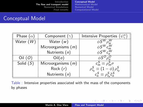
Phase (α) Component (γ) Intensive Properties(ψαγ)

Water (W ) Water (w) φSW ρWw

Microorganisms (m) φSW cWm

Nutrients (n) φSW cWn

Oil (O) Oil(o) φSOρOo

Solid (S) Microorganisms (m) cSm ≡ ρS

mσRock (r) ρS

rb≡ (1− φ) ρS

rp

Nutrients (n) cSn ≡ ρS

rbcS

n

Table : Intensive properties associated with the mass of the componentsby phases





Mathematical Model

I For deriving the equations of the mathematical model theaxiomatic formulation of continuum mechanic systems isapplied [6].

I This axiomatic formulation adopts a macroscopic approach,which considers that the material systems are fully occupiedby particles.

I A continuum system is made of a particle set known asmaterial body, see figure 1.

I The continuum system approach works with the volumeaverage of the body properties and consequently there is avolume called representative elementary volume (REV) overwhich the property averages are valid.





Axiomatic Formulation of Continuum Mechanic Systems

Figure : General scheme of a material body: B (t) is the body withboundary ∂B (t), where n is the outer normal vector, Σ (t) is thediscontinuity surface with a normal vector nΣ and velocity vΣ.






I The continuum approach formulation basically consists in toestablish a one to one correspondence between the extensiveproperties E (t), which are the volume integrals of theintensive properties, for example: the mass, and the intensiveproperties ψ (x, t), which are the physical properties by unit ofvolume, for example: the mass density. Both properties arerelated by the following expression:

E (t) ≡∫

B(t)ψ (x, t) dx, (1)






I Global Balance Equation

dE (t)

dt=

∫B(t)

g (x, t) dx+

∫Σ(t)

gΣ (x, t) dx+

∫∂B(t)

τ (x, t)·ndx

(2)where g (x, t) is the source term in B (t); gΣ (x, t) is the source term

at Σ (t); and τ (x, t) is the vector flux through the boundary ∂B (t).

I Local Balance Equations

∂ψ

∂t+∇ · (ψv) = g +∇ · τ ; ∀x ∈ B (t) (3)

[[ψ (v − vΣ)− τ ]] · nΣ = gΣ; ∀x ∈ Σ (t), (4)

where [[f ]] ≡ f+ − f− is the jump of the function f across Σ (t).






I It is necessary to apply the previous procedure to each component

in each phase, obtaining as many equations as components by

phases we have.

I For the resulting system of equations it is required to specify certain

constitutive laws which are related with the nature of the problem,

for example, the Darcy law in the case of a model of flow in porous

media. These constitutive relationships allow to link the intensive

properties among them and define the flux and source terms.

I Even after this operation it is usually necessary to add some

complementary relationships to obtain a determined system.

I Finally, the model is completed when sufficient initial and boundary

conditions are specified. In this manner we get a well posed

problem, which means that there exists one and only one solution.





The flow model

The flow model is based on the oil phase pressure and totalvelocity formulation given by Chen Z. [7]

I Pressure equation

−∇ ·{λk · ∇pO −

(λW dpOW

c

dSW

)k · ∇SW

}−∇ ·

{(λOρO + λW ρW

)γk · ∇z

}= qO + qW − ∂φ

∂t

(5)

I Saturation equation

φ∂SW

∂t −∇ ·{λW k · ∇pO −

(λW dpOW

c

dSW

)k · ∇SW

}−∇ ·

{(λW ρW γ

)k · ∇z

}+(∂φ∂t

)SW = qW

(6)





The flow model

I Phase velocities

uW = −λf W k · ∇pO + λf W(

dpOWc

dSW

)k · ∇SW − λf W ρW γk · ∇z ;

uO = −λf Ok · ∇pO − λf OρOγk · ∇z ;(7)

Here, uα is the Darcy velocity

uα = −kαrµα

k · (∇pα + ραγ∇z) ;α = O,W (8)

where φ - porosity, k - absolute permeability tensor, Sα -

saturation, να - viscosity, ρα - density, pα - pressure, kαr - relative

permeability, and qα - source term, for each phase α = O,W , |g| -

absolute value of the gravity acceleration, pOWc - capillary oil-water

pressure and z - vertical coordinate.Martın A. Dıaz Viera Flow and Transport Model




The flow model

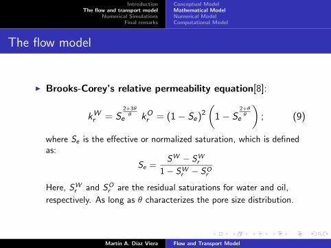
I Brooks-Corey’s relative permeability equation[8]:

kWr = S

2+3θθ

e kOr = (1− Se)2

(1− S

2+θθ

e

); (9)

where Se is the effective or normalized saturation, which is definedas:

Se =SW − SW

r

1− SWr − SO

r

Here, SWr and SO

r are the residual saturations for water and oil,

respectively. As long as θ characterizes the pore size distribution.





The flow model

I Brooks-Corey’s oil-water capillary pressure equation:

pOWc

(SW)

= pt

(SW − SW

r

1− SWr − SO

r

)(−1/θ)

(10)

where pt is the entry or left threshold pressure assumed to be

proportional to (φ/k)1/2.





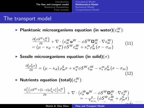
The transport model

I Planktonic microorganisms equation (in water)(cWm ):

∂(φSW cWm )

∂t +∇ ·(cW

m uW − φSW DWm · ∇cW

m

)= (µ− κd − κm

a )φSW cWm + κm

r ρSm (σ − σirr )

(11)

I Sessile microorganisms equation (in solid)(σ):

∂(ρSmσ)∂t = (µ− κd ) ρS

mσ + κma φSW cW

m − κmr ρ

Sm (σ − σirr )

(12)

I Nutrients equation (total)(cWn ):

∂{(φSW +(1−φ)ρS

rbκn

a

)cW

n

}∂t +∇ ·

(cW

n uW − φSW DWn · ∇cW

n

)= − µ

Ym/n

(φSW cW

m + ρSmσ)

(13)Martın A. Dıaz Viera Flow and Transport Model




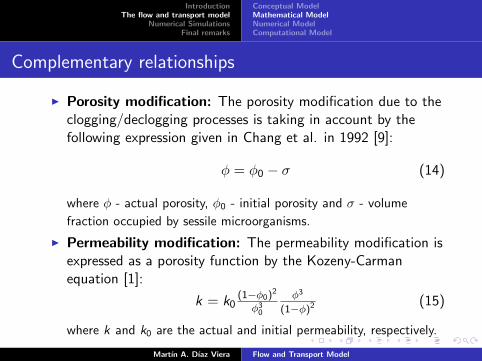
Complementary relationships

I Porosity modification: The porosity modification due to theclogging/declogging processes is taking in account by thefollowing expression given in Chang et al. in 1992 [9]:

φ = φ0 − σ (14)

where φ - actual porosity, φ0 - initial porosity and σ - volume

fraction occupied by sessile microorganisms.

I Permeability modification: The permeability modification isexpressed as a porosity function by the Kozeny-Carmanequation [1]:

k = k0(1−φ0)2

φ30

φ3

(1−φ)2 (15)

where k and k0 are the actual and initial permeability, respectively.





Initial and boundary conditions

I Initial conditions:

pO (t0) = pO0 , SW (t0) = SW

0 ;cW

m (t0) = cWm0, σ (t0) = σ0, cW

n (t0) = cWn0 ;

(16)

I Boundary conditions1. Inlet conditions (constant rate)

uO · n = uW · n = uWin · n;

−[cWγ uW

in − φSW DWγ · ∇cW

γ

]· n = cW

γinuW

in · n, γ = m, n;(17)

2. Outlet conditions (constant pressure)

pO = pOout ,

∂SW

∂n = 0;∂cWγ

∂n = 0, γ = m, n;(18)





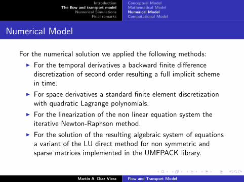
Numerical Model

For the numerical solution we applied the following methods:

I For the temporal derivatives a backward finite differencediscretization of second order resulting a full implicit schemein time.

I For space derivatives a standard finite element discretizationwith quadratic Lagrange polynomials.

I For the linearization of the non linear equation system theiterative Newton-Raphson method.

I For the solution of the resulting algebraic system of equationsa variant of the LU direct method for non symmetric andsparse matrices implemented in the UMFPACK library.





Computational Model

I Once we have established the numerical model for the solutionof the mathematical model its computational implementationis required.

I The realization of the flow model was performed using theCOMSOL Multiphysics r software by the PDE mode ingeneral coefficient form for the time-dependent analysis [10].




Reference case study descriptionSecondary recovery by water injectionEOR by microorganisms and nutrients injection

Reference case study: a waterflooding test in a core

I The reference case study is a waterflooding test in a core thatcan be conventionally divided in two injection steps that aresequentially performed.

I In the first step the oil is displaced by water injection.

I While, in the second one the water is injected withmicroorganisms and nutrients.

I The data used here to simulate both injection steps are takenfrom the published literature [11, 12].





First injection step: secondary recovery by water injection

I Initially, a Berea sandstone core of 0.25 m of length and 0.04m of diameter with homogeneous porosity (φ0=0.2295) andisotropic permeability (k0 = 326 md) set in vertical position,is fully saturated with water.

I The water is displaced by oil injection until the residualsaturation of water is achieved.

I The water is injected from the lower side of the core with aconstant velocity of one foot per day (3.53× 10−6 m/s),while the oil and water are produced at a constant pressure(10 kPa) in the opposite side of the core during 200 hoursuntil a steady state is obtained.

I A summary of the data is given in table 2 which are takenfrom [11] and [12].





Data for the flow and transport model

Parameter Value Parameter ValueCore length L = 0.25 m Core diameter d = 0.04 m

Porosity φ0 = 0.2295 Permeability k0 = 326 md

Water viscosity νW = 1.0 × 10−3 Pa.s Oil viscosity νO = 7.5 × 10−3 Pa.s

Water density ρW = 1.0 g/cm3 Oil density ρO = 0.872 g/cm3

Residual water saturation SWr = 0.2 Residual oil saturation SO

r = 0.15

Production pressure pOout = 10 kPa Brooks-Corey parameter θ = 2

Entry pressure pt = 10 kPa Injection velocity uWin = 1 ft/day

Nutrients dispersion DWn = 0.0083 ft2/day Microorganisms dispersion DW

m = 0.0055 ft2/day

Injected nutrients conc. cWnin

= 2.5 lb/ft3 Injected microorganisms conc. cWmin

= 1.875 lb/ft3

Microorganisms density ρBm = 1000 kg/m3 Irreducible biomass fraction σirr = 0.003

Maximum specific growth µmax = 8.4 day−1 Affinity coefficient Km/n = 0.5 lb/ft3

Production coefficient Ym/n = 0.5 Decay coefficient κd = 0.22 day−1

Adsorption coefficient κma = 25 day−1 Desorption coefficient κm

r = 37 day−1

Table : Data for the flow and transport model taken from [11] and [12].





A 3D view of the finite element discretization mesh

Figure : 1,702 tetrahedral elements, 6,232 degrees of freedom,execution time: 170.179 seg, in a PC with CPU Intel Core2 [email protected] GHz and 4Gb of RAM @1.97 GHz.





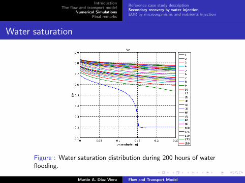
Water saturation

Figure : Water saturation distribution during 200 hours of waterflooding.





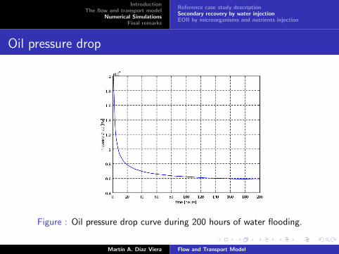
Oil pressure drop

Figure : Oil pressure drop curve during 200 hours of water flooding.





Oil recovery

Figure : Oil recovery curve during 200 hours of water flooding.





Interpretation of results

I It is shown that a water front through the porous medium isformed. The oil displaced by the water front is recovered atthe upper end of the core.

I The head of water breaks through the top of the core justbefore the two hours. It can be observed that the oil pressuredrop (δp ≡ pO

in − pOout) downfalls drastically from 20 kPa to 8

kPa during the first 20 hours, whereas in the next 180 hoursthe oil pressure drop continues downfalling but slowly up to avalue of 5,770 Pa, approximately.

I It is worth to note that the oil recovery curve represents atypical behavior of a recovery process where the porousmedium is strongly oil wet.

I The total recovery of oil is approximately 74%.





Second injection step: EOR by water injection withmicroorganisms and nutrients

I In the second step of the test, microorganisms and nutrientsare injected simultaneous and continuously to the Bereasandstone core through the water phase during 24 hours untila steady state is obtained.

I The intention of this test consists in evaluating the additionaloil production that can be recovered by mechanical effectsbecause of the microbial activity (MEOR).

I As in the first step of the test data are taken from [11] and[12].





A 3D view of the finite element discretization mesh

Figure : 1,702 tetrahedral elements, 15,577 degrees of freedom,execution time: 216.906 seg, in a PC with CPU Intel Core2 [email protected] GHz and 4Gb of RAM @1.97 GHz.





Water saturation

Figure : Water saturation distribution during 24 hours of waterflooding with microorganisms and nutrients.





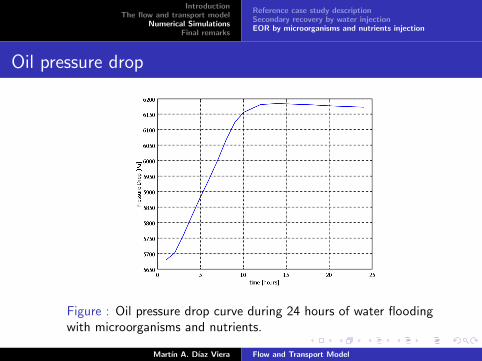
Oil pressure drop

Figure : Oil pressure drop curve during 24 hours of water floodingwith microorganisms and nutrients.





Oil recovery

Figure : Oil recovery curve during 24 hours of water flooding withmicroorganisms and nutrients.





Nutrients and planktonic microorganisms concentrations

Figure : Nutrients (rising from 40 kg/m3) and planktonicmicroorganisms (rising from 30 kg/m3) concentrations, given everyhour, along the vertical axis during 24 hours of water flooding withmicroorganisms and nutrients.Martın A. Dıaz Viera Flow and Transport Model




Sessile microorganisms concentration

Figure : Sessile microorganisms concentrations, given every hour,along the vertical axis during 24 hours of water flooding withmicroorganisms and nutrients.





3D porosity distribution

Figure : 3D porosity distribution after 24 hours of water floodingwith microorganisms and nutrients.





3D permeability distribution

Figure : 3D permeability distribution after 24 hours of waterflooding with microorganisms and nutrients.






I It is observed that water continues displacing the oil throughthe core during the 24 hours of water flooding withmicroorganisms and nutrients.

I It can be seen that there is a slightly increase in the oilpressure drop from 5680 to 6185 Pa. This repressurizationphenomenon is associated with the modification of porosityand, consequently, with the modification of the permeabilitydue to the biomass growth.

I A marginal additional oil recovery of about 0.2% is obtained.






I Stationary state is established around the 6 hours, wherenutrients are almost completely consumed, while at the 24hours approximately an asymptotic value in the concentrationof microorganisms is reached.

I The maximum planktonic and sessile microorganismsconcentration values are achieved in cW

m = 48.85 kg/m3 andσ = 1.1% at 0.074 m and 0.041 m, respectively.

I The variations in σ are reflected directly in porosity andpermeability changes, where the minimum values are achievedin a zone around 0.041 m from the core bottom.




Final remarksFuture workReferencesAcknowledgements

Final remarks

I In this work a quite general flow and transport model inporous media was implemented using the standardformulation of the finite element method to simulatelaboratory tests at core scale and under controlled conditions.

I This model was successfully applied to a reference case studyof oil displacement by the injection of water follows by theinjection of water with microorganisms and nutrients, usingdata taken from the published literature.





Final remarks

I In this paper, the porosity and permeability modification dueto the variation in the biomass distribution along the core wasinvestigated.

I The resemblance of the porosity (φ) and permeability (k)spatio-temporal distributions of the form of the sessilemicroorganisms concentration (σ), can be attributed to thesimplicity of the porosity and permeability relationshipsapplied.

I The application of more realistic dependence functions is anopen issue.





Final remarks

I The observed repressurization phenomenon associated withthe modification of porosity and permeability due to thebiomass growth could be used to plug highly permeable zonesto redirect the flow and to increase the oil sweep efficiency.

I Regarding the marginal additional recovery produced duringthe EOR microbial process, less than 1%, it can not bedirectly attributed to the mechanical effects such as thepressure increase due to microbial growth.





Future work

I To model other effects such as: rock wettability, viscosity ν,relative permeability kr and capillary pressure pc curvesmodification because of the bioproducts action over fluids androck, further experimental investigation is required, toquantify in terms of constitutive relationships the interactionbetween petrophysical and fluid properties as a function ofbioproducts concentrations.





References

P. C. Carman, Flow of gases through porous media, Butterworth, London, (1956).

Jacob Bear, Dynamics of fluids in porous media, Dover, USA, (1972).

Gaudy, A.F., Jr. and E.T. Gaudy, Microbiology for environmental scientists and engineers, McGraw-Hill

Book Co., USA, (1980).

Corapcioglu M.Y. and A. Haridas, “Transport and fate of microorganisms in porous media: A theoretical

investigation”, Journal of Hydrology, 72, 149-169, (1984)

Lappan, E.R. and Fogler, H.S., “Reduction of porous media permeability from in situ Leuconostoc

mesenteroides growth and dextran production”, Biotechnol. Bioeng., 50 (1), 6-15, (1996)

M. B. Allen, I. Herrera and G. F. Pinder, Numerical modeling in science and engineering, John Wiley &

Sons., USA, (1988).

Z. Chen, G. Huan and Y. Ma, Computational methods for multiphase flows in porous media, SIAM, USA,

(2007).

R. Brooks and A. Corey, “Hydraulic Properties of Porous Media”, of Colorado State University Hydrology

Paper, 3, Colorado State University, (1964).

M.M.Chang, R. S. Bryant, A.K. Stepp and K.M. Bertus, “Modeling and Laboratory Investigations of

Microbial Oil Recovery Mechanisms in Porous Media”, DE/93 000105, NIPER-629, (1992).

COMSOL Multiphysics, Modeling Guide Version 3.4, COMSOL AB, USA, (2007).

H. Hoteit and A. Firoozabadi, “Numerical modeling of two-phase flow in heterogeneous permeable media

with different capillarity pressures”, Advances in Water Resources, 31, 5673, (2008).

M. M. Chang, F. T-H. Chung, R. S. Bryant, H. W. Gao and T. E. Burchfield, “Modeling and laboratory

investigation of microbial transport phenomena in porous media”, SPE, 22845, 299-308, (1991).





Acknowledgements

I This work was supported by the project D.00417 of the IMPOil Recovery Program.





Thank you

¿Questions , comments?


a flow and transport model in porous media for … viera...media for microbial enhanced oil recovery...

Documents