a finite volume method for transport of contaminants in porous media

ofnd

numberlindane,

es,nd tendtermsof the

nation.of soil

by the, sharpion ofrd finite

Applied Numerical Mathematics 49 (2004) 291–305www.elsevier.com/locate/apnum

A finite volume method for transport of contaminantsin porous media

Enrico Bertolazzia, Gianmarco Manzinib,∗

a Dipartimento di Ingegneria Meccanica e Strutturale, Università di Trento, via Mesiano 77, I-38050 Trento, Italyb Istituto di Analisi Numerica IAN-CNR, via Ferrata 1, I-27100, Pavia, Italy

Abstract

A cell-centered finite-volume method is proposed to solve the unsteady reactive diffusive transporta contaminant in porous media. Two theoretical properties of the analitical solution, namely non-negativity amaximum principle, are mentioned and their implication on the approximation method are discussed. 2004 IMACS. Published by Elsevier B.V. All rights reserved.

Keywords: Contaminant transport; Finite volumes; Least square reconstructions

1. Introduction

In recent years the problem of groundwater contamination has achieved increasing attention. Aof contaminants are often found in subsurface environments: herbicides and pesticides (atrazine,etc.), heavy metals (Pb, Zn, Cr, Cu, etc.), radionuclides (90Sr,135Cs, uranium and a number of its isotopetc.). These are particularly harmful for soils and groundwater, because they are highly toxic ato accumulate to the bottom of aquifers and sit there for a long time. Different problems arise inof horizontal and vertical spreading of these contaminants, their interaction with the soil, durationcontamination period, possibility of remediation, containment and/or attenuation of the contamiIn this context, the role of modeling has been of major importance in predicting future scenariosand aquifer contamination and designing human remediation intervention strategies.

The macroscopic models for the solute transport in a porous media are usually describedadvection–diffusion equation. When the groundwater flow is dominated by the advective termmoving fronts of solute concentration tend to appear in the analytical solution. The formatthese strong gradient regions makes difficult the numerical approximation process by standa

* Corresponding author.E-mail address: [email protected] (E. Bertolazzi).

0168-9274/$30.00 2004 IMACS. Published by Elsevier B.V. All rights reserved.doi:10.1016/j.apnum.2003.12.008

292 E. Bertolazzi, G. Manzini / Applied Numerical Mathematics 49 (2004) 291–305

difference and finite element methods. Indeed, spuriousO(1) non-physical oscillations known as Gibbs’phenomena, can develop and deteriorate the accuracy of the numerical solution. To overcome these

te in then, the

hniqued finite6,4] andtting ofplicit,implicit,on. Asxplicitplicit

insteadnd therm isiffusionains theured byiscrete

entionework.y. The–Lewyacer in

ically,

tion of

spatial

phenomenona, shock-capturing numerical schemes have been developed and widely investigalast two decades. These schemes try to combine numerical stability with minimal artificial diffusioform of this latter one being dependent on the adopted approach [15].

The advection and the diffusion terms are usually discretised in a different way, each with the tecdeemed most appropriate, and coupling of quite different methods, such as finite volumes anelements, is not unusual. For example, we can mention the Eulerian–Lagrangian schemes [1the fully Eulerian Godunov mixed methods [6–9,14]. These schemes are based on the splithe advection and the diffusion terms into two separate partial differential equations. A time-exspatially second order accurate Godunov method is basically used to treat advection, and a time-spatially second order accurate mixed finite element method is used for modeling the diffusipointed out in [14], this approach lessens the stability constraint which is connected with the ediscretization of the diffusion term, but also allows the possibility of using more effective exschemes for the advection one.

The numerical schemes that is presented and numerically investigated in this paper makesusage of a finite volume approach for the simultaneous discretisation of both the advective adiffusive flux on the interface boundary of a suitable set of control volumes. The advective teapproximated by using an upstream technique, while a central scheme is adopted for the done. Formal second-order accuracy is achieved by employing a linear reconstruction that maintapproximate cell-average values computed by the scheme. The stability of the scheme is ensusing an appropriate slope limiter, which is combined with the reconstruction in order to satisfy a dversion of a maximum principle and of a non-negativity property of the analytical solution.

The paper is organized as follows. In Section 2 we show the governing equations and we mthe analytical properties that we want to focus on. In Section 3 we discuss the finite volume framIn Section 4 we illustrate the reconstruction algorithm required to attain second-order accuractheoretical properties of the scheme are validated in Section 5 for different Courant–Friedrichs(CFL) and Peclet(Pe) numbers on a time-dependent sample problem, that is the movement of a tra semi-infinite column. Finally, in Section 6 we draw the conclusions.

2. Advective and diffusive transport

Let us indicate byΩ the computational domain where the model equation is defined. MathematΩ is a connected polygonal domain inR2 defined by a closed (1-D) surface∂Ω . We assume thatΩ ishomogeneously filled by a porous medium where the bulk flow takes place. The governing equathe phenomenon we are interested in reads as

(RC)t + ∇ · (VC − D∇C) = S, in R+ × Ω. (1)

Eq. (1) describes the time-dependent advective–diffusive transport of a contaminant whoseconcentration distribution is denoted byC(t,x). The contaminant is passively advected byV(t,x), whichis an assigned convection field;D(t,x) is the diffusion tensor,R(t,x) is the retardation factor, andS(t,x)

is the contaminant production/consumption source term [11].

E. Bertolazzi, G. Manzini / Applied Numerical Mathematics 49 (2004) 291–305 293

This model problem is completed by furnishing an initial solution, that is the spatial distribution of thecontaminant at timet = 0 within the domainΩ ,

e. Thets,

ount forample,

ditionsntration

discreteumericals that

oblem

em

C(0,x) = C0(x), x ∈ Ω,

and by specifying the boundary conditions that can be either of Dirichlet-type or of Neumann typborder∂Ω may be partitioned into the union of two non-overlapping and possibly empty subseΓD

andΓN , where respectively Dirichlet- and Neumann-type conditions are specified:∂Ω = ΓD ∪ ΓN . Theboundary conditions are given by

Dirichlet: C = gd onR+ × ΓD,

Neumann: D∇C · n = gn onR+ × ΓN,

(2)

wheregd andgn are assumed to be smooth functions. Furthermore, the source term, which can accboth production of contaminants, for example, due to pollution leakage, and consumption, for exdue to a remediation intervention, takes the following rather general form,

S(t,x,C) = −A(t,x,C)C(t,x) + B(t,x,C),

whereA(t,x,C) andB(t,x,C) are also supposed smooth and non-negative functions.

2.1. Basic analytical results

Under some general assumptions on the initial contaminant distribution and the boundary conimposed on the model problem, it is possible to prove the non-negativity of the contaminant conceand a global maximum principle [12]. This is stated by the two following propositions.

Proposition 1 (Non-negativity).

If C0(x) 0, gd(t,x) 0, and gn(t,x) > 0then 0 C(t,x), for t > 0, and x ∈ Ω.

Proposition 2 (Global maximum principle).

If C0(x) 0, gd(t,x) 0, gn(t,x) > 0, and S = 0,

then 0 C(t,x) M(t), for t > 0, and x ∈ Ω,

where M(t) = max

supx∈Ω

C0(x), supτ∈(0,t )

supx∈Γ D

gd(τ,x).

In the rest of the paper we illustrate the design of a cell-centered FV method that ensures aversion of these properties. Basically, the discrete version of Proposition 1 guarantees that the napproximation ofC is a non-negative field, while the discrete version of Proposition 2 guaranteethe numerical approximation ofC satisfies a stability constraint.

3. The finite volume formulation

The design of our FV method starts as usual by reformulating in an integral form the model prdefined by Eqs. (1) and (2) on a set of closed and non-overlapping control volumesTi ∈ Th, whereTh isa conformal triangulation ofΩ [10]. Integrating Eq. (1) overTi , applying the Gauss divergence theorand imposing when required the boundary conditions given in (2), we have


∂

∂t

∫R(· ,x)C(· ,x)dx +

∑j∈T (i)

∫ [C(· ,x)V(· ,x) − D(· ,x)∇C(· ,x)

] · nij d

y,

inedited

appear

lationured fornin the

ntrol ofh cell, a

Tih eij

+∑

j ′∈T dh (i)

∫eij

[gd(·, x)V(·, x) − D(· ,x)∇C(· ,x)

] · nij d

∑j ′∈T n

h (i)

∫eij

C(· ,x)V(· ,x) · nij − gn(·, x)d

=∫Ti

[−A(C(·, x)

)C(·, x) + B

(C(·, x)

)]dx, for everyTi ∈ Th. (3)

In (3) Th(i) is the index set of volumes adjacent toTi , eij is the edge shared byTi and Tj , i.e.,eij = Ti ∩ Tj , andT d

h (i) andT nh (i) the index set of the edges ofTi located on the domain boundar

i.e.,eij = Ti ∩ ∂Ω . The symbolnij denotes the vector that is normal to the edgeeij and oriented fromTi

to Tj when the edge is internal, or outward-directed when the edge is on the boundary.The finite volume method is formulated on each volumesTi ∈ Th by the equation

|Ti|drici

dt+

∑j∈Th(i)

[Gij (c)︸︷︷︸

convection

+Hij (c)︸︷︷︸diffusion

]+

∑j∈T ′

h(i)

Fij ′(c)︸︷︷︸boundary

= Si(c)︸︷︷︸sourve

, (4)

where we indicate the numerical flux integral terms corresponding to the ones in (3). In (4)ri is theTi

cell-average of the retardation factorR.We denote the piecewise-linear FV approximation ofC by c(· ,x). The restriction ofc(· ,x) to the cell

Ti ∈ Th is

ci(· ,x) = ci + Gi (c) · (x − xi ), x ∈ Ti ,

whereci is the finite-volumeO(h2) approximation of the cell average ofC within Ti ,

ci ≈ 1

|Ti |∫Ti

C(· ,x)dx,

andGi is a cell-centeredO(h) estimate of the solution gradient. The gradient approximation is determby using the FV cell average inTi and the ones within the surrounding cells and a special limreconstruction algorithms. The limiter is introduced to control the numerical oscillations that canin the approximation process. Major details about these issues are described in the next section.

3.1. Least-square vertex reconstruction

The definition of the discrete advective and diffusive fluxes in the finite volume scheme formurequires the estimate of the solution gradient at the cell interfaces. Second-order accuracy is enssmooth solution when the gradient approximations are at leastO(h). We make a distinction betweethe approximate gradients that take part in the advective flux definition from the ones that arediffusive one, because the formers are monotonized by a suitable TVD constraint to provide cothe numerical oscillations. Thus, the scheme requires four different gradient estimations for eaccell-centered one to whom a limiter may be applied, and three edge-centered ones.


These quantities must be estimated using the only information available from the scheme, that is theapproximation of the cell-averaged solution values. Consequently, a proper linear reconstruction process

radientrem toerical

e caseith

nt

recover

set of

ion

lds the

g

must be devised.Gradients are recovered from cell averages by approximating the integral of the solution g

on the cellTi and on different subsets of this latter one. Then, we apply the Gauss–Green theotransform any surface integral into a closed 2-D contour integral. Finally, by considering a numquadrature rule on each closed integration path we obtain the computational scheme.

The integration path coincides with the triangular cell for the cell-average gradient. Instead, in thof the gradient centered at the edgeeij , the integration path coincides with the internal sub-triangle wvertices the centroidxi of Ti and the two vertices ofeij . The mid-point rule provides the final gradieformula.

Thus, this strategy requires the knowledge of the vertex values. Consequently, an algorithm tothese latter ones from cell averages is necessary.

This algorithm is based on alinear approximation in the sense of the least square method of thetriplets

(xi, yi, ci), i ∈ Th(α),

whereTh(α) is the set of cells sharing the vertexα. That is, we seek for the following linear representatof the solution at each vertexα with coordinates(xα, yα)

cα = a + bxα − cyα,

wherea, b andc are the minimizers of

E(a, b, c) =∑

i∈Th(α)

λαi(a + bxi + cyi − ci)2,

and λαi is an assigned set of normalized non-negative weights. The least square method yievertex valueca in the form of the weighted average of the centroid valuesci ,

cα =∑

j∈Vh(α)

ωαjcj , (5)

where the set of weightswαj can be written in terms of the initial set of weightsλαiωαj = λαj

(1+ (

xα − xGα

)TS−1

α

(xj − xG

α

)).

In this relation we have introduced the formal inverse of the 3× 3 matrix

Sα =∑

j∈Th(α)

λαj

(xj − xG

α

)(xj − xG

α

)T

and theλ-weighted barycenter of the set of triangles incident the vertexα

xGα =

∑j∈Th(α)

λαjxj .

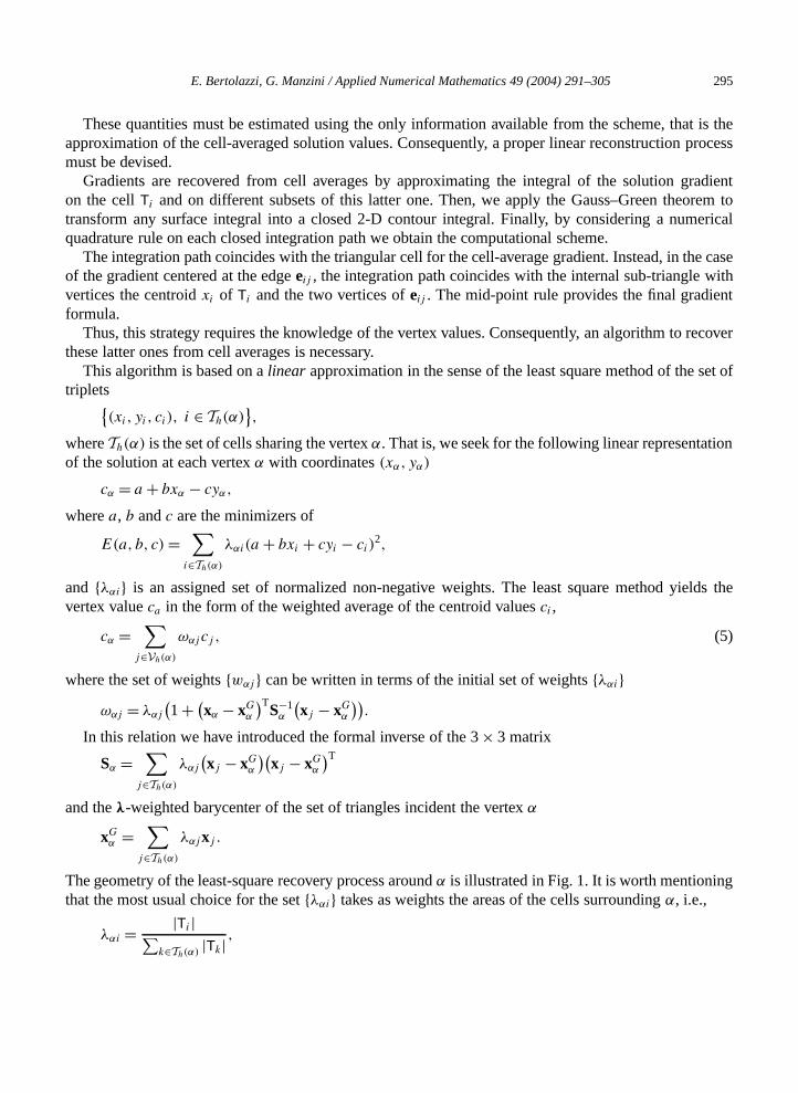
The geometry of the least-square recovery process aroundα is illustrated in Fig. 1. It is worth mentioninthat the most usual choice for the setλαi takes as weights the areas of the cells surroundingα, i.e.,

λαi = |Ti |∑k∈Th(α) |Tk| ,


in very

rsors

la TVD

Fig. 1. Geometry of the least-square method; the cell centroidsxi () and theλ-weighted barycenterxGα (∗) are indicated.

but the final weightswαj produced in this case by the least square method may be negative or attalarge values when the mesh is strongly stretched [13]. However, a choice ofλαi that produces strictlypositive weightswαj is always possible.

3.2. Limited gradient reconstruction and discretization of the advection term

The piecewise-constant gradientGi(c) within the cell|Ti|, is recovered by using the formula

Gi(c) = i

1

2|Ti |R[cα(xβ − xγ ) + cβ(xγ − xα) + cγ (xα − xβ)

].

This gradient is such that the vector(Gi(c),1) is orthogonal to the plane for the 3-D vecto(xα, cα), (xβ, cβ) and (xγ , cγ ), where xα,xβ,xγ are the counterclock-wise ordered position vect(counterclock-wise ordered) vertices ofTi .

The scalar limiting factori is the largest real number in[0,1] such that

(i) minci, cj ci (· ,xij ) maxci, cj , eij ∈ E Ih ;

(ii) minci,gdij ′ ci(· ,xij ′) maxci,gdij ′ , eij ′ ∈ EDh ;

(iii) (Gi(c) · nij ) · gnij 0, |dij Gi(c) · nij | |gnij |, eij ′ ∈ ENh , anddij = ∫

eijD(· ,x)d.

This limiting strategy ensures that the recovered gradient is null whenci is a local minimum or a locamaximum. In this way, the linear reconstructed solution is monotonized, thus providing also thatstability constraint is satisfied.

The advection term in Eq. (3) is discretized by using a standard upwind technique. We have

Gij (C) = ν+ij ci (· ,xij ) + ν−

ij cj (· ,xij ) = ν+ij (· ,xij ) − ν+

ij cj (· ,xij )

≈∫eij

C(· ,x)V(· ,x) · nij d, j ∈ Th(i),


ps, that

r

r

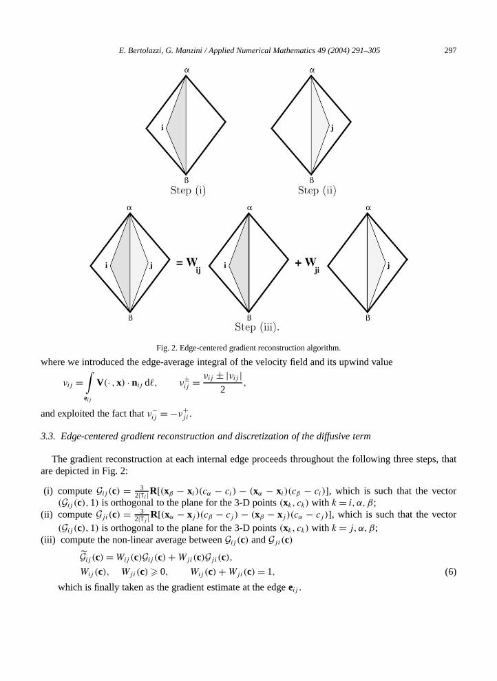
Fig. 2. Edge-centered gradient reconstruction algorithm.

where we introduced the edge-average integral of the velocity field and its upwind value

νij =∫eij

V(· ,x) · nij d, ν±ij = νij ± |νij |

2,

and exploited the fact thatν−ij = −ν+

ji .

3.3. Edge-centered gradient reconstruction and discretization of the diffusive term

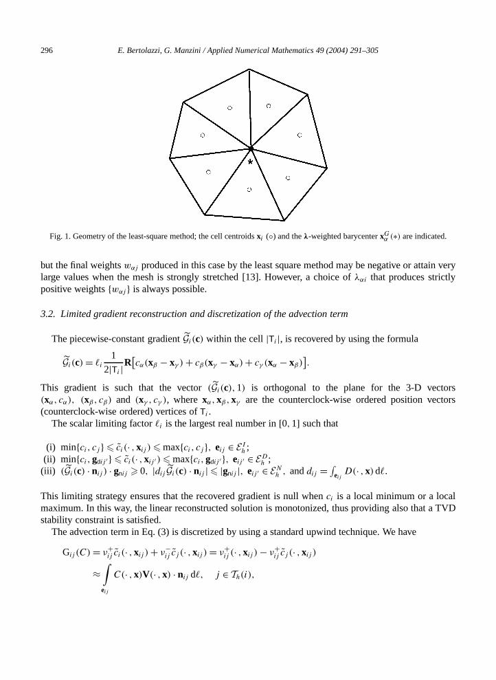
The gradient reconstruction at each internal edge proceeds throughout the following three steare depicted in Fig. 2:

(i) computeGij (c) = 32|Ti |R[(xβ − xi)(cα − ci) − (xα − xi)(cβ − ci)], which is such that the vecto

(Gij (c),1) is orthogonal to the plane for the 3-D points(xk, ck) with k = i, α,β;(ii) computeGji(c) = 3

2|Tj |R[(xα − xj )(cβ − cj ) − (xβ − xj )(cα − cj )], which is such that the vecto(Gij (c),1) is orthogonal to the plane for the 3-D points(xk, ck) with k = j,α,β;

(iii) compute the non-linear average betweenGij (c) andGji(c)

Gij (c) = Wij (c)Gij (c) + Wji(c)Gji(c),

Wij (c), Wji(c) 0, Wij (c) + Wji(c) = 1, (6)

which is finally taken as the gradient estimate at the edgeeij .


The termsWij (c) in Eq. (6) are the scalar weights of the final average and are generally assumed todepend on the set of neighbour cell-averaged and vertex-reconstructed values.

e

entify

liptic

ey the

This approach generalises the “diamond scheme” average [5], which corresponds to a choice of thweights which depends only on the area of the closest cells,

Wij (c) = |Ti|/(|Ti| + |Tj |

),

but is independent from the cell-average solution values. Different and originalnon-linear averagestrategies can be envisaged following the criteria established in [2]. For example, if we first idthe minimum contribution to the edge-centered gradientWij from the cellsTi and Tj , the remaindercontribution can be weighted by using

Wij (c) = |gji (c)|

|gij (c)|+|gji(c)|, if∣∣gij (c)

∣∣ + ∣∣gji(c)∣∣ > 0,

12, if

∣∣gij (c)∣∣ + ∣∣gji(c)

∣∣ = 0

andgij (c) = Gij (c) · nij . It is shown in [2] that this approach yields a numerical scheme for pure elproblems that satisfies a maximum principle.

Let cij be the linear interpolation ofcα and cβ at the pointxij ∈ eij , orthogonal projection of thcentroid xi onto eij . Substituting the expression (5) in Eq. (6) and taking into account properldefinition of Gij (c) given in step (iii), the component of this latter orthogonal toeij can be written as

dij Gij (c) · |eij |nij = hij (c)(cij − ci

), for all eij ∈ Eh, (7)

wheredij is the edge-average viscosity

dij = 1

|eij |∫eij

D(· ,x)d,

andhij (c) is a bounded non-negative scalar function of the cell averagesc.An algebraic manipulation makes possible to re-write the r.h.s. of Eq. (7) in the form

hij (c)(cij − ci

) = hj i(c)cj − hij (c)ci, for all eij ∈ E Ih .

The discrete diffusive flux is finally defined as

Hij (c) = hij (c)ci − hj i(c)cj ≈ −∫eij

D(· ,x)∇C(· ,x) · nij d.

3.4. Numerical approximation of the source term

The volume production/consumption source term is numerically discretized in every cellTi ∈ Th bythe second-order quadrature formula

Si(c) = |Ti|B(· ,xi , ci) − |Ti|A(· ,xi , ci)ci

=∫Ti

B(· ,x, c(· ,x)

) − A(· ,x, c(· ,x)

)c(· ,x)dx +O

(h3

).


4. Formal properties of the FV formulation

itable

(4)

ge

bothfs are

ng two

In this section we re-formulate the FV scheme (4) in a more compact form. Introducing a sudefinition of the matrix operatorsG, G(c), H(c),F, F(c) and the vectorsf, f(c)—see [3] for the details—the discrete cell-wise advective and the diffusive flux balance can be rewritten like[

Gc − G(c)c]i=

∑j∈Th(i)∪T ′

h(i)

Gij (c),

[H(c)c

]i=

∑j∈Th(i)∪T ′

h(i)

Hij (c), (8)

while the contribution from boundary edges becomes[Fc − F(c)c − (

f − f(c))e]i=

∑j∈T ′

h(i)

Fij (c). (9)

The r.h.s. source also takes a matrix–vector form as

S(c) = bS(c) − A(c)c (10)

Using the definitions (8), (9), and (10), the final matrix–vector form is obtained for the PV scheme

d

dt(Mc) + N(c)c = N(c)c + b(c). (11)

In Eq. (11), the termb(c) = f − f(c) + bS(c) collects all the of contributions from the boundary edfluxes. We have also introduced the non-linear matrix operatorsN(c) = F + G + H(c) + A(c) andN(c) = F(c) + G(c). Under the assumptions given in the previous section it is possible to showN(c) and N(c) possess strong properties, that we formalize in the next propositions. The proostraightforward.

Proposition 3 (Properties of the matrix operators).

(1) N(c) is an M-matrix;(2) N(c) is a Stieltjes matrix.

Two discrete analogues of Propositions 1 and 2 also hold. These are stated by the followipropositions.

Proposition 4 (Non-negativity).The analytical property 1 becomes:

if ci(0) 0, for all Ti ∈ Th;gdα

(t) 0, for all α ∈ V ′h, t > 0;

gnij(t) 0, for all eij ∈ EN

h , t > 0;then 0 ci(t), for all Ti ∈ Th, t > 0.


Proposition 5 (Global maximum principle).The analytical property 2 becomes:

ifferentcuracy,constantvolume

and the

in thelocityof

of this

umbers,quallyesh case.

n

if ci(0) 0, for all Ti ∈ Th;gdα

(t) 0, for all α ∈ V ′h, t > 0;

gnij(t) = 0, for all eij ∈ EN

h , t > 0;bS(c) = 0, t > 0;

then 0 ci(t) M(t), for all t > 0.

5. Numerical results

In this section we present and discuss the performance of the finite volume scheme on two dsets of numerical experiments. The first set is aimed at illustrating that the second order of acwhich is theoretically expected, is achieved when the convergence rate is measured by taking aviscosity value on different refined meshes. The second set is aimed at illustrating that the finiteapproximated solution is practically unaffected on a wide range of Peclet numbers, from about 3.4× 101

to ∞. This range corresponds to viscosity values passing from a situation where the advectiondiffusion terms are almost balanced to a strongly advective flow—no diffusive terms are present.

The benchmark problem is the same for both sets of numerical experiments and consistsadvection–diffusion transport of a contaminant in a semi-infinite column. A constant advective veis considered which is given byV = (v,0)T. The viscosityD is assumed to be a scalar multiplethe identity matrix and its value ranges throughout zero—purely advective transport—to 1× 102. Theintegration domain is a unitary lenght rectangle. The boundary conditionsC = 1 atx = 0 andC = 0 forx = ∞ are imposed. Zero concentration is used as the initial solution state. The analytical solutionproblem is given by [1]

C(t,x) = 1

2

[erfc

(x − vt

2√

Dt

)+ exp

(vx

D

)erfc

(x − vt

2√

Dt

)]. (12)

The behavior of the scheme is characterized as a function of two grid related dimensionless nnamely theCFL and thePe numbers. These numbers are usually introduced for schemes on espaced Cartesian meshes, and their definitions are generalised as follows to the unstructured mTheCFL number is defined as

CFL = t supi

[p(Ti)

|Ti |]

supj

|νij |,

wherep(Ti) is the perimeter and|Ti| the area of theith triangleTi . ThePe number is the ratio betweethe advective and the dispersive terms and takes the form

Pe = CFL

γ,

where the dispersion numberγ is given by

γ = |D|t supi

1

|Ti| .


Finally, in all of the numerical experiments discussed in this section the time-dependent equation (11) isdiscretised in time by the first-order accurate Euler implicit scheme, that is by approximating the time

e tables

tes arele

derivative term by

d

dt(Mc) = Mn cn+1 − cn

t+O(t). (13)

The results of the first set of numerical experiments are summarised in Tables 1 and 2. Thesalso report the parameters of all the calculations.

In order to consider grid orientation effects, the approximation errors and the convergence raevaluated on grids of two different types, labeled by “A” and “B” and illustrated in Fig. 3. Six spatiarefinement levels are considered and labeled by the indexl in the first column of Tables 1 and 2. At th

Fig. 3. Grids of typeA andB.

Table 1Grid A: parameters and results

l Nd Ymax CFL Pe Eabs E rel Rate

1 10 0.5 0.91 28.51 3.25× 10−2 1.56× 10−1 –2 20 0.25 0.45 14.26 1.02× 10−2 6.91× 10−2 1.173 40 0.125 0.23 7.13 2.36× 10−3 2.27× 10−2 1.604 80 6.25× 10−2 0.11 3.56 3.43× 10−4 4.67× 10−3 2.285 160 3.125× 10−2 5.7× 10−2 1.78 6.99× 10−5 1.34× 10−3 1.806 320 1.5625× 10−2 2.85× 10−2 0.89 1.06× 10−5 2.81× 10−4 2.25

Table 2Grid B: parameters and results

l Nd Ymax CFL Pe Eabs E rel Rate

1 10 0.5 0.61 38.50 2.83× 10−2 1.35× 10−1 –2 20 0.25 0.31 19.25 5.90× 10−3 4.01× 10−2 1.753 40 0.125 0.15 9.63 1.04× 10−3 9.98× 10−3 2.004 80 6.25× 10−2 7.7× 10−2 4.82 2.13× 10−4 2.90× 10−3 1.785 160 3.125× 10−2 3.85× 10−2 2.41 4.42× 10−5 8.89× 10−4 1.776 320 1.5625× 10−2 1.92× 10−2 1.20 8.21× 10−6 2.23× 10−4 1.92


coarsest grid levell = 1, the computational domain is the rectangle[0,1] × [0,0.1], and is discretisedinto four layers of rectangular elements that are further subdivided into two triangles for grids of type

igthoints ofved and

isions.ycuracy,

r tond 2

ight

ns, thus

problemschemesariosstronglyn termby thisability of

are takeners

A or four triangles for grids of typeB. When passing from a grid level to the next finer one, the heof the computational domain is halved and the refined mesh is obtained by connecting the midpthe three edges of each triangle. In this way, the triangle shape at the different levels is presereach refined mesh actually covers the rectangular domain[0,1] × [0,Ymax], with Ymax ranging from 0.1to 1.5625× 10−2. The second column of Tables 1 and 2 reports the number of rectangular sub-divNd of the mesh along the longitudinal direction, the third column reports the values ofYmax for each case

In all these calculations we take the constant viscosity valueD = 1×10−2 and a constant unit velocitv − 1 (in the proper dimension units). In order to observe the theoretical second-order spatial acwe employ the timestept = x2. Consequently, thePe number is halved in passing from a coarsea finer grid level, while theCFL number tends to zero. The forth and the fifth column of Tables 1 areport their values.

The sixth and seventh columns report the values of the absolute errorEabs and the relative errorE rel

with respect to the analytical solution given in Eq. (12),

Eabs=√√√√ ∑

i∈Th(Ω)

|Ti|3

∣∣ci − C(t,xi )∣∣2, (14)

and

E rel = Eabs√∑i∈Th(Ω)

|Ti |3

∣∣C(t,xi )∣∣2

. (15)

These errors are evaluated at the timeT = 0.5, that is before the concentration front reaches the rboundary.

The last column gives the rate of convergence measured on the relative error,

Rate(l, l + 1) = log2E rel

l

E rell+1

. (16)

It is evident from these tables that second-order convergence rate is attained in nearly all of the ruconfirming the theoretical approximation accuracy of the scheme.

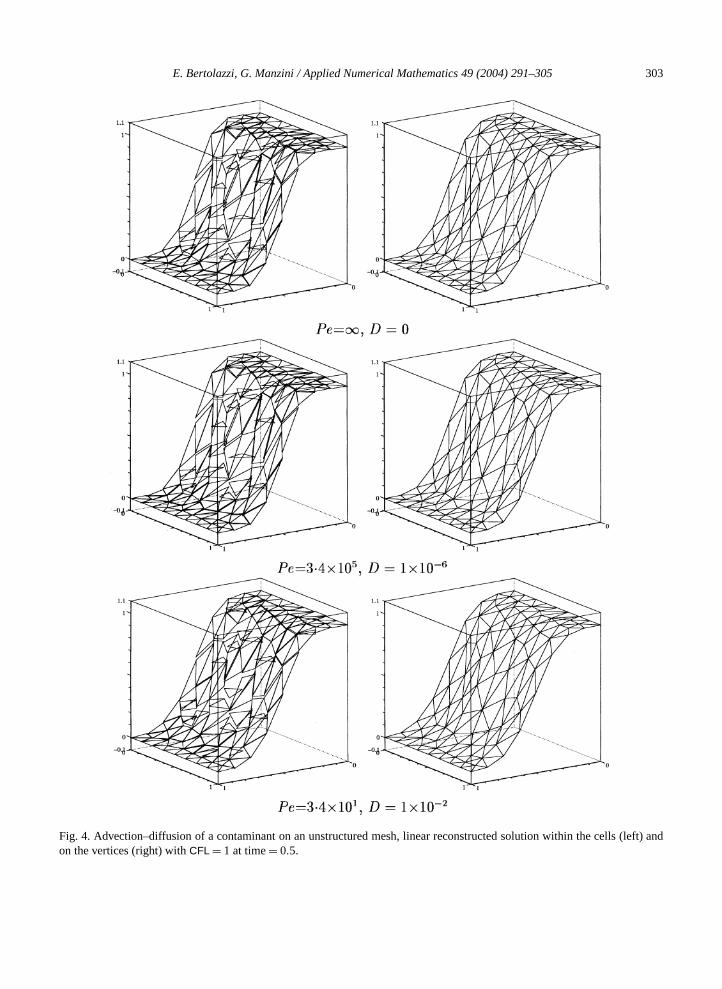
The second set of numerical experiments that has been performed on the semi-infinite columnillustrates the good behavior of the scheme at different viscosity and Peclet numbers. Thehas been tested by changing the viscosity value from zero to 10× 10−2, that is for Peclet numberranging from∞ to about 3.4× 101. As already discussed at the beginning of this section, the scencorresponding to these extreme cases are quite different. The former case corresponds to aconvective transport where the diffusive term is totally absent, while in the latter case the advectiois almost balanced by the diffusive term. Nonetheless, the finite volume approximation providedscheme appears to be nearly unaffected over this wide range of situations, thus witnessing the stthe present approach.

Fig. 4 shows the results on three time-dependent calculations, that are performed withCFL = 1 on anunstructured mesh of 162 triangles, 259 edges and 98 vertices. The scalar viscosity values thatinto account in these calculations areD = 0 andD = 1 × 10−2, which corresponds to the two extremsituations discussed above, and the intermediate caseD = 1× 10−6. The corresponding Peclet numbe


left) and
Fig. 4. Advection–diffusion of a contaminant on an unstructured mesh, linear reconstructed solution within the cells (on the vertices (right) withCFL = 1 at time= 0.5.


are indicated in the figure subcaptions. The linear reconstructed solutions are shown at timeT = 0.5, thatis before the advancing contaminant front reaches the end of the rectangular computational domain. On

he right

ximateand 5.

minants withinmulate

strongr quite

nciple.ation

structedom isroceed-orderthe

d methodort to a

sionale-based

l.

ar

r,9.n–

(1990)

l. 28 (5)

the left, we show the approximate solution reconstructed within the mesh triangular cells and on tthe reconstructed solution on the mesh vertices.

In all of these calculations we also checked the non-negativity of the cell-averaged approsolution and the maximum principle thus confirming the theoretical predictions of Propositions 4

6. Conclusions

A FV scheme is proposed to solve the time-dependent advection–diffusion for the contatransport in porous media. This scheme is based on a special limited reconstruction for gradientcells and at mesh edges. The introduction of a suitable matrix-like formalism allows us to reforthe scheme in a more compact way. The matrix operators that appear in the new formulation showproperties (M-matrices, Stieltjes matrices). Using these properties it is possible to prove that undegeneral assumptions the discrete solution is non-negative and there holds a global maximum pri

The resulting finite volume scheme is conservative and formally linearly exact in the approximof the cell-averaged solution values.

The introduction of a solution feedback by a suitable edge-centered average of the recongradients implies that this scheme is inherently non-linear, even if the model problem to whapplied is a linear one. Since this non-linearity makes very difficult the convergence analysis, we pin this work to a direct experimental testing of the method. The method shows optimal secondconvergence in a suitable discreteL2 norm for the approximation of the solution cell averages andvertex-centered least square reconstructed values. The solution obtained by using the proposeis experimentally shown to be stable over a wide range of scenarios, from purely advective transpbalanced advection-diffusion case.

Finally, it is worth mentioning that this methodology can be directly extended to the three-dimenequation by reformulating either the vertex-centered least-square reconstruction and the edggradient reconstruction on three-dimensional tethrahedra.

References

[1] J. Bear, Hydraulics of Groundwater, McGraw-Hill, New York, 1979.[2] E. Bertolazzi, Numericalconservation and discrete maximum principle for elliptic pdes, Math. Models Methods App

Sci. 8 (1998) 685–711.[3] E. Bertolazzi, G. Manzini, Limiting strategies for polynomial reconstructions in finite volume approximations of the line

advection equation, Appl. Numer. Math. 49 (2004) 277–289, this volume.[4] V. Casulli, Eulerian–Lagrangian methods for hyperbolic and convection dominated parabolic problems, in: C. Taylo

D.R.J. Owen, E. Hinton (Eds.), Computational Methods for Nonlinear Problems, Pineridge, Swansea, 1987, p. 23[5] Y. Coudière, J.-P. Vila, P. Villedieu, Convergence rate ofa finite volume scheme for a two-dimensional convectio

diffusion problem, Modél Math. Anal. Numér. 33 (1999) 493–516.[6] C.N. Dawson, Godunov-mixed methods for immiscible displacement, Internat. J. Numer. Methods Fluids 11 (7)

835.[7] C.N. Dawson, Godunov-mixed methods for advection flow problems in one space dimension, SIAM J. Numer. Ana

(1991) 1282.


[8] C.N. Dawson, Godunov-mixed methods for advection–diffusion equationsin multidimensions, SIAM J. Numer.Anal. 5 (30) (1993) 1315.

e time-

erical

dation

e

ed grids,

r,

pace time

[9] C.N. Dawson, High-resolution upwind-mixed finite element methods for advection diffusion equations with variablstepping, Numer. Methods Partial Differential Equations 11 (1995) 525.

[10] R. Eymard, T. Gallouët, R. Herbin, Finite volume methods, in: P.G. Ciarlet, J.L. Lions (Eds.), Handbook of NumAnalysis, vol. VII, North-Holland, Amsterdam, 2000, pp. 713–1020.

[11] C. Gallo, G. Manzini, A fully coupled numerical model for two-phase flow with contaminant transport and biodegrakinetics, Comm. Numer. Methods Engrg. 17 (2001) 325–336.

[12] D. Gilbarg, N.S. Trudinger, Elliptic Partial Differential Equations of Second Order, Springer, Berlin, 2001. Reprint of th1998 edition.

[13] P. Jawahar, H. Kamath, A high-resolution procedure for Euler and Navier–Stokes computations on unstructurJ. Comput. Phys. 164 (2000) 165–203.

[14] A. Mazzia, L. Bergamaschi, M. Putti,A time-splitting technique for the advection–dispersion equation in groundwateJ. Comput. Phys. 157 (2000) 181–198.

[15] K.W. Morton, Numerical Solution of Convection–Diffusion Problems, Chapman and Hall, London, 1996.[16] S.P. Neuman, A Eulerian–Lagrangian numerical scheme for the dispersion convection equation using conjugate s

grids, J. Comput. Phys. 41 (1981) 270.

a finite volume method for transport of contaminants in porous media

Documents