a csr asset pricing model
TRANSCRIPT

A CSR ASSET PRICING MODEL
Souad LAJILI JARJIRa
aUniversity Paris-Est, IRG (EA 2354)
Aya NASREDDINEb
bEBS Universitat
Marc DESBANc
cUniversity Paris-Est, IRG (EA 2354)
Revised May 2017
Abstract. This study challenges widely used factor models (one, three, four and five factor models) in
explaining stock returns in Europe and proposes an innovative corporate social responsibility (CSR) factormodel. Our sample covers monthly past returns on 18 European stock markets over thirteen years (June
2002 to May 2015). We examine the empirical relationship between the return and the extra-financial
notation of CSR in Europe. We observe that the less responsible firms have higher risk adjusted returns,on average, than the most responsible ones. We reveal a new risk premium associated to extra-financial
notation priced by the market. We propose a parsimonious two-factor model including both the market
and the CSR premia that outperforms existing asset pricing models in describing CSR rated firms’ returns.Unlike previous models, our model is validated according to the GRS test.
Introduction
In this paper, we propose to study the efficient hypothesis of financial markets regarding to extra-
financial notation. Our objective is to make a link between two well-documented fields in financial
literature: asset pricing and corporate social performance (CSP). This study explores a new issue
related to the consideration of financial markets for extra-financial notation. To our best knowledge,
no paper deals with this particular issue. Regarding the asset pricing field of research, the linear relation
between the expected rate of return of an asset and its risk dates from the fifties but remains one of the most
fundamental assumptions made in finance. Following the seminal work of Markowitz (1952) [36], finance
has known a substantial development since the outbreak of the first Capital Asset Pricing Model (Sharpe,
1964 [49]; Lintner, 1965 [33]; Mossin, 1966 [42] and Black, 1972 [6]). Despite this success, a large body of
research criticizes the single factor model, unsatisfying to explain securities past returns as it relies on an
unobservable market portfolio (Roll, 1977 [46]). A few years later, Levy and Roll (2010) [32] attest that many
conventional market proxies could be perfectly consistent with the CAPM. Creating an asset pricing model
fully describing stocks returns will probably stay one of the hardest challenges in finance. The huge body of
the empirical work on the Capital Asset Pricing Model remains usually inconclusive and fails to rationalize
Key words and phrases. Asset Pricing, Size effect, Value premium, Momentum, Risk factors, Three, Four and Five factorModels, Extra-financial rating, Corporate Social Responsibility and Anomalies. JEL classification: G12.
1

S. Lajili Jarjir, A. Nasreddine and M. Desban
market anomalies not explained by the plain vanilla CAPM (since there are several versions, see Cochrane,
2000 [15]). Among all the criticisms, the most celebrated one is the work by Fama and French (1993) [19] who,
in a series of papers, propose to consider the existence of additional risk factors as a consistent hypothesis.
Carhart (1997) [11] proposes a four factor model adding a portfolio of winners minus losers to the three
factor model. Recently, Fama and French (2015) [21] suggest a five-factor asset pricing model which capture
the size, value, operating profitability and investment patterns in average US stock returns.
For corporate social performance, Moskowitz (1972) [41] was one of the pioneers in the CSP research field.
He finds empirically that firms that have strong enough management to uphold their social responsibilities
also have the skill and caliber to run a company with superior financial performance, making it attractive
to investors, and thus rising the price of its stock up. Since then, the relationship between corporate social
responsibility and accounting-based indicators of financial performance has been extensively examined by
researchers with mixed findings (Waddock and Graves, 1997 [53]; Allouche and Laroche, 2006 [2]; Nelling and
Webb, 2009 [43]). Developed in Europe only starting from the beginning of the 21st century, the European
Commission (2001) defines corporate social responsibility as ”a concept whereby companies integrate social
and environmental concerns in their business operations and in their interaction with stakeholders on a vol-
untary basis”. A firm’s level of corporate social responsibility (CSR) may be measured by several dimensions,
including good treatment of employees, reducing the level of environmental negative impact of production or
philanthropic activities. While the number of academic studies in this area has also increased substantially
in recent years, no clear consensus has yet emerged concerning whether investment in socially responsible
stocks or funds is favorable or detrimental to returns. Holme and Watts (2000) [27] defines Corporate social
responsibility as ”the commitment of business to contribute to sustainable economic development, working
with employees, their families, and the local community and society at large to improve their quality of life”.
Since our concern lies with the identification of the appropriate asset pricing model for CSR involved
firms, we challenge widely used factor models (one, three, four and five factor models) in explaining stock
returns in Europe and we propose an innovative CSR factor model. Our results shed light on two main
contributions. First, we reveal a risk premium associated to extra-financial notation priced by the market.
Second, we propose a parsimonious model including two risk factors that outperforms existing asset pricing
models in describing CSR rated firms’ returns. Adding CSR premium to the beta is sufficient to explain
screened stocks by extra-financial agencies.
This paper proceeds as follows: Section I gives a theoretical background of the pricing models. Section II
introduces the data sets used and the applied methodology. Section III summaries results of empirical tests
and section IV presents conclusions.
2
A CSR Asset pricing model
1. Literature review
In financial markets, observing and understanding patterns in returns is and will always be an important
issue. Since the fifties, many economic models were introduced to specify the relationship between return
and risk. Indeed, the Capital Asset Pricing Model CAPM (Sharpe, 1964 [49]; Lintner, 1965 [33]; Mossin,
1966 [42] and Black, 1972 [6]) is the most widely used model because of its simplicity. It assumes that
investors respect the Markowitz mean-variance criterion in choosing their portfolios. The beta revolution
had a significant impact on the academic and non-academic financial community. Other factor pricing
models attempt to explain the cross-section of average asset returns as the Inter-temporal Capital Asset
Pricing Model (Merton, 1973 [40]), the Arbitrage Pricing Model (Ross, 1976 [47]) and the inter-temporal
capital asset pricing model based on consumption (Rubinstein, 1976 [48]; Lucas, 1978 [35]); Breeden, 1979
[9], Mehra and Prescott 1985 [39] among others). Many anomalies are identified from empirical failures of the
CAPM. Fama and French 1993 [19] propose a three factor model including size and book to market effects
in explaining returns. Carhart (1997) [11] proposes a four factor model adding a portfolio of winners minus
losers to the three factor model. Besides, Fama and French (2012) [20] explore size, value and momentum
anomalies in a sample of international stock returns by comparing global and local models. They reject global
models in explaining regional returns and find that local models give acceptable descriptions of local average
returns. Recently, Fama and French (2015) [21] suggest a five-factor asset pricing model which capture the
size, value, profitability and investment patterns in average US stock returns.
The relationship between corporate social responsibility and financial performance has been extensively
examined by researchers with mixed findings.
Positive association between the two concepts: Waddock and Graves 1997 [53] document that
lower implicit costs by socially irresponsible actions induce higher explicit costs for the firm. In addition,
the potential benefits for the firm are higher than the costs of CSP.
Good management can be considered as an explanation for this positive relationship. Besides, slack
resources resulting from good financial performance can be used to improve social performance. Lastly,
having both good management and slack resources can create a virtuous circle between CSP and financial
performance. Holme and Watts (2000) [27] found that CSR was not just relevant business sense, but also
helped contribute to the long-term growth, success and survival of the company. Cox et al. (2004) [16] and
Graves and Warddock (1994) [25] show that poor corporate social responsibility can lead to a decrease in
the number of long-term institutional investors holding these stocks. Considering only the environmental
dimension of the CSR, Feldman et al. (1997) [22] and Derwall et al. (2004) [17] find that the highest
3

S. Lajili Jarjir, A. Nasreddine and M. Desban
portfolios in terms of environmental score significantly outperforms the lower ranking portfolios in terms of
stock returns.
Other empirical studies investigate the issue of firm characteristics, CSR and financial markets. Lourenco
et al. (2012) [34] indicate that large profitable firms can be penalized by the market due to their low level
of CSP. Otherwise, Godfrey et al. (2009) [24] introduce the risk management hypothesis to understand
a possible relationship between firm characteristics and market reaction. Indeed, managers who decide to
improve the CSR of their firms can create value for their shareholders. Furthermore, Oikonomou et al.
(2012) [45] emphasize the importance of the market conditions in the determination of the nature and the
strength of the CSP-risk relationship. They argue that there exist both a negative but weakly relation
between CSR and systematic firm risk; and a positive and strong relationship between corporate social
irresponsibility and financial risk. Lackmann et al. (2012) [31] conclude that reaction to an increase in the
reliability of sustainability information is stronger for firms with high systematic investment risk, financial
leverage, and levels of opportunistic management behavior. The relation between CSR and firm value can
be explained based on the corporate governance theory. According to the stakeholder theory (Freeman, 1984
[23]; Clarskon, 1995 [14]), firms should use CSR as an extension of effective corporate governance mechanisms
to resolve conflicts between managers and non-investing stakeholders. In this case, CSR is value enhancing.
Firms develop intangible and valuable assets considered as source of competitive advantage (Hillman and
Keim, 2001 [26]). Jo and Harjoto (2012) [30] show that corporate governance positively influences CSR, and
CSR increases firm value. Their results support the conflict-resolution hypothesis, and therefore stakeholder
theory, as opposed to overinvestment argument.
Negative association between the two concepts: Contrary to stakeholder theory and according to
the agency theory (Jensen and Meckling, 1976 [29]), insiders have an interest in overinvesting in CSR if doing
so provides private benefits of reputation building as good social citizens, possibly at a cost to shareholders
(Barnea and Rubin, 2010 [3]). Cheng et al. (2014) [13] find empirical evidence supporting the argument
that managers of large US firms enjoy private benefits from investing in CSR. In this case, CSR is value
destroying.
Brammer et al. (2005) [8] find that the composite CSR score is significantly and negatively related to stock
returns, but the poor financial reward offered by these firms is mainly attributable to their good performance
with employment, and environmental measures. They conclude that empirical evidence provided by the
authors suggests that there is a negative impact of socially responsible UK firms on their stock returns and
link this finding to the increased costs incurred from the additional measures they are required to fulfill.
Indeed, the cost of socially responsible behavior can explain the negative sign of the relationship. This
argument is consistent with the neoclassical theory. Brammer et al. (2005) [8] somehow confirmed the
4
A CSR Asset pricing model
proposition of Vance (1975) [52] who find evidence to support the negative effect of CSR firm strategies on
stock performance and link this finding to the competitive disadvantage induced by CSR expenses. This
point of view was also confirmed by McWilliams and Siegel (2001) [38]. Based on Carhart (1997) [11] four
factor model, Bauer et al. (2002) [4] show that both German and US ethical funds underperform their
benchmark in terms of their risk-adjusted returns, although similar UK funds achieve slight outperformance.
However, authors also noticed a learning effect that is at work thanks to an improvement of ethical fund
managers over time.
Inconclusive association between the two concepts: A last point of view supposes that, under
some assumptions concerning the markets and well-defined property rights, an equilibrium should develop
overtime engaging in expenditure on CSR involved firms leading thus to indistinguishable returns to socially
responsible and irresponsible firms of course for a given level of risk and other firm characteristics. This
neutral relationship can be explained by the efficient market hypothesis, which assumes that publicly available
information is immediately incorporated into prices (Shleifer, 2000 [50]). Becchetti et al (2012) [5], using a
large sample of US firm forecasts, find that CSR contributes to make financial markets efficient. Besides,
because of the measurement problems related to the Corporate Social Performance (CSP), some authors
(Ullman, 1985 [51]) believe that there is no link between social and financial performance. Rather than
seeing CSR as a voluntary action, institutional theory suggests seeking to place CSR within a wider field
of economic governance characterized by different modes, including the market, regulations, formal and
informal rules, norms (Brammer et al., 2012 [7]). Because firms are embedded in different national systems,
they may face divergent internal and external pressures to engage in CSR activities (Aguilera et al. 2007 [1];
Campbell, 2007 [10]). Matten and Moon (2008) [37] suggest that unlike the voluntary and explicit forms of
CSR found in liberal economies, CSR is likely to be more implicit within coordinated market economies.
So far, most empirical research on CSR has focused mainly on the relationship between CSP and firm’s
financial performance as well as the links between CSP and firm’s characteristics. Our objective is to assess
how investors price the quality of extra-financial information. Considering a European database gathering
firms with available extra-financial notation, we shed light on the existence of a CSR premium. The latest
is integrated in a two factor asset pricing model that seems to be suitable for the description of CSR rated
firms’ returns.
2. Data and variables
2.1. Database. We study monthly past returns on the European market through 18 different countries
from June 2002 to May 2015. We use DATASTREAM to extract and construct our data base. Like Fama
and French, financial firms and stocks with negative book-to-market ratio are eliminated from the sample
5

S. Lajili Jarjir, A. Nasreddine and M. Desban
comprising in fine 12,144 firms listed on Euronext Stock Exchange market. We retain firms listed at least
for three years. We include delisting one when available. Subsequently, we independently sort our sample to
assign stocks to three groups regarding their Asset4 extra-financial notations 1 (good, neutral and bad) and
to three book-to-market (Panel A), operating profitability (Panel B), and investment groups (Panel C)2. We
label these portfolios with two letters: The first letter describes the book-to-market (high [H ], neutral [N ]
and low [L]), operating profitability (robust [R], neutral [N ] and weak [W ]) and investment (conservative
[C ], neutral [N ] and aggressive [A]). Like Fama and French (1992) [18], we form our variables at the end of
June in year t by using information from fiscal year-end t− 1 from DATASTREAM. The different strategies
tested are monthly value-scaled. We consider a holding period return from the beginning of June of year t
to the end of July of year t+ 1. Allocation of portfolios is annually updated.
2.2. Explanatory variables. Several independent variables are used in our time series regressions:
• The Market Premium [RM −Rf ] is the excess return of the European market.
• The Small Minus Big portfolio [SMB ] corresponds to the difference between the average monthly
stock returns of the three portfolios of small capitalizations (SL, SM and SH) and the three with
big capitalizations (BL,BM and BH).
• The High Minus Low portfolio [HML] corresponds to the difference between the average monthly
stock returns of the two portfolios with the highest book-to-market ratios (SH and BH) and the two
with the lowest ratios (SL and BL)3.
• The Winners Minus Losers portfolio [WML] is the return of a long strategy on stocks with high
past returns (winners) minus the return of a short strategy on firms with low past returns (losers).
Every month t, stocks are sorted into 3 groups according to their cumulative returns between month
t − 12 and t − 2. Then we compute the value-weighted returns of the winner and loser portfolios.
The WML factor is thus the spread.
• The Robust Minus Weak portfolio [RMW ] corresponds to the difference between the average
monthly stock returns of the two highest profitable portfolios (SR and BR) and the the two lowest
(SW and BW )4. We retain the definition of the operating profitability ratio of Hou, Xue and Zhang
(2015) [28] and Fama and French (2015) [21]5.
1Asset4 is one of the bigger providers of ESG (environmental, social, governance) information.2book-to-market ratio is obtained by inverting market-to-book [MTBV]. Revenues minus cost of goods sold, minus selling, general,
and administrative expenses [EBITDA: WC18198], minus interest expense [WC01251] all divided by book equity [WC05491]constitute our operating profitability ratio. Finally, investment is defined as the annual change in gross property, plant, and
equipment added of the annual change in inventories [Total Asset: WC02999] between t− 2 and t− 1 all divided by the lagged
book value of total assets of t− 2.3HML = (SH + BH)− (SL + BL)/24RMW = (SR + BR)− (SW + BW )/25It corresponds to the revenues minus cost of goods sold, minus selling, general, and administrative expenses, minus interestexpense all divided by book equity. The definition given by Novy-Marx (2012) [44] and Chen and Zhang (2010) [12] is respectively
6

A CSR Asset pricing model
• The Conservative Minus Aggressive portfolio [CMA] corresponds to the difference of the average
monthly returns on portfolios with high asset growth rates, designated agressive (SA and BA) and
portfolios with conservative firms (SC and BC)6. Like Chen and Zhang (2010) [12], Hou, Xue and
Zhang (2015) [28] and Fama and French (2015) [21] the investment proxy is the annual change in
gross property, plant, and equipment added of the annual change in inventories between t − 2 and
t− 1 all divided by the lagged book value of total assets of t− 2.
• The Bad Minus Good portfolio [BMG ] corresponds to the difference between the average monthly
stock returns of the two portfolios of stocks with the best extra-financial notations (the top 30%)
and the worst one (the lower 30%). Portfolio allocations in the beginning of t+ 1 are based on the
grades in the end of t. Those strategies are maintained one year and are then rebalanced.
2.3. Dependent variables. Three sets of portfolios named ”panels”are used as dependent variables. At the
end of each year, stocks are classified into three CSR groups regarding their extra-financial notation (good,
neutral and bad). Stocks are subsequently allocated independently to three book-to-market groups (Panel
A), three investment groups (Panel B), three operating profitability groups (Panel C). The intersections of
the two sorts produce 9 value-weighted portfolios per panel corresponding to the left hand side variables.
2.4. Summary statistics. On average, firms with the highest monthly excess returns have bad CSR grades.
Indeed, we report a 1.41% and a 1.42% average monthly return for firms with bad notation and respectively
high and low B/M classification compared to a 0.65% and 0.94% for firms with good CSR grade (see Table
1, panel A). This category is also found to be the riskiest since we record a 16.69% average monthly standard
deviation for firms with bad notation and high B/M compared to firms with good notation and high B/M
with a 7.55% average standard deviation. Also firms with bad notation and low B/M have on average 7.83%
monthly standard deviation compared to an average monthly standard deviation of 3.76% for firms with good
notation and low B/M. Form descriptive statistics, there is no obvious relationship between average return
and B/M classification. However, value stocks seem to be riskier than growth stocks on average. Besides,
the higher average number of firms is recorded for companies classified to be neutral in terms of notation
and B/M whereas the lowest average number of firms concerns companies with bad notation and high B/M.
Also, firms with good CSR notation and low B/M seem to have higher average market capitalization.
Concerning portfolios sorted by investment and CSR notation, descriptive statistics in panel B of Table
2 show that, firms with the highest average returns have bad notations. Moreover, firms that are considered
to be aggressive have always higher average stock return than conservative ones. However, aggressive firms
measured by the gross profits (revenues minus cost of goods sold) to its assets and by the income before extraordinary dividedby last quarter’s total assets. Those different definitions constitute robustness tests driving us to select the Fama and Frenchdefinition.6CMA = (SC + BC)− (SA + BA)/2
7

S. Lajili Jarjir, A. Nasreddine and M. Desban
are less risky than conservative ones based on average standard deviation. Whereas, firms with bad notation
display higher average monthly standard deviation than good graded firms. Also, the higher number of firms
in average is for companies classified to be neutral in terms of notation and investment whereas the lowest
average number of firms concerns aggressive companies with good notation. Also, aggressive firms with good
CSR notation seem to have higher average market capitalization.
Turning this time to portfolios sorted by profitability and CSR notation, we also record a higher average
monthly stock return for firms with bad CSR notation compared to companies with good notation. Indeed,
we report a 1.28% and a 1.23% average monthly return for firms that are respectively robust and weak
having bad notation compared to a 0.55% and 0.04% average monthly returns for firms with good notation
while being robust and weak respectively in terms of profitability classification. Robust firms seem to have
higher average return than weak ones. Moreover, the latest is riskier than robust firms since we record a
higher monthly return standard deviation for weak firms compared to robust companies. Still, firms with bad
CSR notation have on average a higher standard deviation compared to good graded companies. The higher
number of firms in average is for robust companies classified to be neutral in terms of notation whereas the
lowest average number of firms concerns weak companies that have good notation. Additional descriptive
statistics are reported in Table 3 panel C.
Table 4, 5 and 6 reports Pearson and Spearman correlation matrix of variables monthly excess returns.
Strategies considered in table 4 panel A are built based on B/M and CSR grade independent classifications.
Correlations appear to be low between the considered portfolios and the risk factors: market, SMB, HML,
WML, orthogonalized WML, RMW, CMA, and BMG. Especially, the constructed BMG appears to be
positively correlated with market factor, SMB and HML whereas it is negatively linked to RMW, CMA
and WML. These correlations are still low (0.27, 0.21, 0.17, -0.22, -0.07 and -0.15 respectively). We also
notice that the market factor as well as HML and BMG have a generally positive correlation with the tested
portfolios whereas the correlation appears to be generally negative between the latest and SMB, RMW,
CMA and WML factors. The same results are found for portfolios constructed based on investment and
CSR notation and for strategies built based on profitability and CSR notation classifications. Correlations
are reported respectively in table 5 and 6 respectively for the panels B and C.
Table 7 reports summary statistics of factors monthly returns. For market factor, SMB and HML, we
measure an average monthly return of 0.7%, 0.163% and 0.214% respectively. Moreover, RMW, CMA and
WML factors record a 0.293%, 0.175 and 0.803 average monthly return. BMG factor presents the higher
average monthly return (1.187%) but displays also the highest standard deviation among the tested risk
factors (Market premium, SMB, HML, RMW, CMA and WML).
8

A CSR Asset pricing model
3. Empirical results
3.1. Time series regressions results for B/M-CSR portfolios: From Panel A of Table 8, Table 9,
Table 10, Table 11 and Table 12, betas are positive and significant for all portfolios and for all asset pricing
models tested. The latest is increased for portfolios with low B/M when adding additional risk factors to
the one factor model. In Table 9 (Panel A), SMB factor is negative and significant for firms with good CSR
notation whereas it is positively and significantly linked to firms with bad notation (except for portfolios
with high B/M ratio). Except Bad graded firms, HML coefficients in table 9 are positive and significant for
value portfolios and negative and significant for growth portfolios. Moreover, as shown in table 10 (Panel
A), WML factor is almost always negative. It is significant for portfolios with high B/M and good notation
and for portfolios with low B/M and bad CSR grade. The same finding for WML applies to RMW and
CMA factors as shown in Table 10 (Panel A). However, in Table 12 (Panel A), BMG factor coefficient is
positive and significant for portfolios of bad graded firms whereas it is negative but not always significant
for portfolios of good graded firms. This finding shows that there is CSR premium for companies that are
classified as bad graded in terms of CSR. Table 14 displays adjusted R squared for CAPM, 3FM, 4FM, 5FM
and the proposed CSR pricing model. From Panel A, One can notice that adjusted R squared are improved
particularly for portfolios of bad graded firms. For these portfolios, the highest adjusted R squared are given
by the CSR model.
3.2. Time series regressions results for investment-CSR portfolios: From Panel B of Table 8, Table
9, Table 10, Table 11 and Table 12, betas are positive and significant for all portfolios and for all asset pricing
models tested. Table 9 (Panel B) shows negative and significant SMB coefficients for firms with good CSR
notation whereas it is positively and significantly linked to firms with bad notation (except for conservative
firms). Except Bad graded firms, HML coefficients in Table 9 (Panel B) are positive and significant for
conservative portfolios and negative but not significant for aggressive portfolios. Moreover, as shown in
Table 10 (Panel B), WML factor is negative and significant for portfolios that are classified as conservative
in terms of investment. The same finding for WML applies to RMW and CMA factors (see Table 11 Panel
B). However, BMG factor coefficient is positive and significant for portfolios of bad graded firms whereas it
is negative but not always significant for portfolios of good graded firms (Table 12 Panel B). From Table 14
(Panel B), one can notice that adjusted R squared are improved for portfolios of bad graded firms especially
for aggressive and conservative firms.
3.3. Time series regressions results for profitability-CSR portfolios: From Panel C of Table 8, Table
9, Table 10, Table 11 and Table 12, betas are positive and significant for all portfolios and for all asset pricing
models tested. Except for weak profitability firms, SMB factor is negative and significant for firms with good
9

S. Lajili Jarjir, A. Nasreddine and M. Desban
CSR notation whereas it is positively and significantly linked to firms with bad notation. Moreover, HML
coefficients in table 8 are positive and significant for robust portfolios. However, when introducing WML,
CMA and RWM, the HML factor loses its significance (as shown in tables 10 and 11). Moreover, as shown
in table 10, WML factor is negative and significant for all strategies except for the portfolio of robust and
good graded firms. The same finding for WML applies to RMW factor in table 11. CMA factor is always
negative and significant except for the firms that are robust in terms of profitability and at the same time
bad graded in terms of CSR. However, BMG factor coefficient is positive and significant for portfolios of bad
graded firms whereas it is negative and significant for portfolios of good graded firms. From Table 14, one
can notice that adjusted R squared are improved for portfolios of bad graded firms.
3.4. Gibbons, Ross and Shanken statistic results: Table 13 displays GRS statistic values for 10 asset
pricing models. Each model is a combination of the market premium factor and one or several other factors
among SMB, HML, WML, RMW, CMA, and our constructed BMG model. Panel A, Panel B and Panel C
of table 13 reports GRS statistic for portfolios classified by B/M-CSR notation, Investment-CSR notation
and Operating profitability-CSR notation respectively. Models with the lowest GSR statistic all contain
BMG factor. Moreover, on average, model 8 presents the lowest GRS test when considering together the
three portfolio classifications. Indeed, GRS test statistics are below the critical value for respectively Panel
A (1.984), Panel B (1.881) and Panel C (1.191).
4. Conclusion
This paper shed light on the negative relationship between the return and the corporate social respon-
sibility proxied by extra-financial notation in Europe from June 2002 to May 2015 (13 years). We cover a
long period since the early 2000s development of extra-financial notation. To our best knowledge, our study
is pioneer in exploring this field under the asset pricing dimension.
Since our concern lies with the identification of the appropriate asset pricing model for CSR involved
firms, we challenge, among others, widely used factor models: one, three, four and five factor models.
We propose a well specified two-factor model including a new risk premium related to corporate social
responsibility succeeding easily the Gibbons, Ross and Shanken test. Considering 27 investment strategies
based on CSR, book-to-market, investment and operating profitability, both market and CSR premia explain
returns without size, value, momentum, operating profitability and investment factors. Both CSR funds and
asset managers can use our local European two-factor model for performance measurements and expected
return computation. Using this model allows also to integrate the corporate social responsibility dimension
in corporate valuation. Most responsible firms will have lower discount factor increasing their market values.
10

A CSR Asset pricing model
For future research, our paper can be extended to different issues in finance. First, it is interesting to
challenge our results with different extra-financial notation agencies. Second, we can investigate how financial
market practitioners consider or not the existence of extra-financial notation in their pricing. Finally, since
the US market remains the most documented in asset pricing field, testing a CSR model would be definitely
an innovative issue.
References
[1] R. V. Aguilera, J. Ganapathi, D. E. Rupp, and C. A. Williams. Putting the s back in corporate social responsibility: A
multilevel theory of social change in organizations. Academy of Management Review, 32(3):836–863, 2007.
[2] J. Allouche and P. Laroche. The relationship between corporate social responsibility and corporate financial performance:
a survey. Allouche, J. (Ed.), Corporate Social Responsibility: Performance and Stakeholders, 2006.
[3] A. Barnea and A. Rubin. Corporate social responsibility as a conflict between shareholders. Journal of Business Ethics,
97:71–86, 2010.
[4] R. Bauer, K. Koedijk, and R. Otten. International evidence on ethical mutual fund performance and investment style
mimeo. In Limburg Institute of Financial Economics, Maastricht University, 2002.
[5] L. Becchetti, R. Ciciretti, I. Hasan, and N. Kobeissi. Corporate social responsibility and shareholder’s value. Journal of
Business Research, 65(11):1628–1635, 2012.
[6] F. Black. Capital market equilibrium with restricted borrowing. Journal of Business, (45):444–55, 1972.
[7] S. Brammer, G. Jackson, and D. Matten. Corporate social responsibility and institutional theory: new perspectives on
private governance. Socio-Economic Review, 10:3–28, 2012.
[8] S. Brammer and S. Pavelin. Corporate community contributions in the united kingdom and the united states. Journal of
Business Ethics, 56:15–26, 2005.
[9] D. Breeden. An Intertemporal Asset Pricing Model with stochastic consumption and investment opportunities. Journal of
Financial Economics, (7):265–96, 1979.
[10] J. Campbell. Why would corporations behave in socially responsible ways? an institutional theory of corporate social
responsibility. Academy of Management Review, 32(3):946, 2007.
[11] M. Carhart. On persistence in mutual fund performance. The Journal of Finance, 52(1):57–82, March 1997.
[12] L. Chen and L. Zhang. A better three-factor model that explains more anomalies. The Journal of Finance, 65(2):563–595,
April 2010.
[13] I. H. Cheng, H. Hong, and K. Shue. Do managers do good with other people’s money? Chicago Booth Paper, pages 12–47,
2014.
[14] M. Clarskon. A stakeholder framework for analyzing and evaluating corporate social performance. Academy of Management
Review, 20:92–117, 1995.
[15] J. H. Cochrane. Asset Pricing. Princeton University Press, 2000.
[16] P. Cox, S. Brammer, and A. Millington. An empirical examination of institutional investor preferences for corporate social
performance. Journal of Business Ethics, 52(1):27–43, 2004.
[17] J. Derwall, N. GA¼nster, R. Bauer, and K. Koedijk. The eco-efficiency premium puzzle mimeo. Rotterdam School of
Management, Erasmus University, 2004.
11

S. Lajili Jarjir, A. Nasreddine and M. Desban
[18] E. F. Fama and K. R. French. The cross section of expected stock returns. The Journal of Finance, 47(2):427–65, June
1992.
[19] E. F. Fama and K. R. French. Common risk factors in the returns on stocks and bonds. Journal of Financial Economics,
33:3–56, 1993.
[20] E. F. Fama and K. R. French. Size, value, and momentum in international stock returns. Journal of Finanacial Economics,
(105):457–472, 2012.
[21] E. F. Fama and K. R. French. A five-factor asset pricing model. Journal of Financial Economics, 116:1–22, 2015.
[22] S. J. Feldman, P. A. Soyka, and P. G. Ameer. Does improving a firsm’s environmental management system and environ-
mental performance result in a higher stock price? Journal of Investing, 6(4):87–97, 1997.
[23] R. Freeman. Strategic management: A stakeholder approach. Massachusetts: Pitman Publishing Inc., 1984.
[24] P. C. Godfrey, C. B. Merrill, and J. M. Hansen. The relationship between corporate social responsibility and shareholder
value: An empirical test of the risk management hypothesis. Strategic Management Journal, 30:425–445, 2009.
[25] S. B. Graves and S. A. Waddock. Institutional owners and corporate social performance. The Academy of Management
Journal, 37(4):1034–1046, 1994.
[26] A. Hillman and G. D. Keim. Shareholder value, stakeholder management, and social issues: what’s the bottom line?
Strategic Management Journal, 22(2):125–139, 2001.
[27] R. Holme and P. Watts. Corporate social responsibility: Making good business sense. In World Business Council for
Sustainable Development: Geneva, 2000.
[28] K. Hou, C. Xue, and L. Zhang. A comparison of new factor models. Working papers, 2015.
[29] M. Jensen and W. Meckling. Theory of firm: Managerial behavior, agency costs, and capital structure. Journal of Financial
Economics, 3:305–360, 1976.
[30] H. Jo and M. Harjoto. The causal effect of corporate governance on corporate social responsibility. Journal of Business
Ethics, 106:53–72., 2012.
[31] J. Lackmann, J. Ernstberger, and M. Stich. Market reactions to increased reliability of sustainability information. Journal
of Business Ethics, 107:111–128, 2012.
[32] M. Levy and R. Roll. The market portfolio may be mean/variance efficient after all. Review of Financial Studies, 23:2464–
2491, 2010.
[33] J. Lintner. The valuation of risk assets and the selection of risky investments in stock portfolios and capital budgets. Review
of Economics and Statistics, (47):13–37, 1965.
[34] I. Lourenco, M. Branco, J. D. Curto, and Eugenio. How does the market value corporate sustainability performance?
Journal of Business Ethics, 108:417–428, 2012.
[35] R. Lucas. Asset prices in an exchange economy. Econometrica, 46(6):1429–45, November 1978.
[36] H. Markowitz. Portfolio selection. Journal of Finance, (7):77–91, March 1952.
[37] D. Matten and J. Moon. ’implicit’ and ’explicit’ csr: A conceptual framework for a comparative understanding of corporate
social responsibility. Academy of Management Review, 33:404–424, 2008.
[38] A. McWilliams and D. Siegel. Corporate social responsibility: A theory of the firm perspective. The Academy of Manage-
ment Review, 26(1):117–127, January 2001.
[39] R. Mehra and E. Prescott. The equity premium: A puzzle. Journal of Monetary Economics, (15):145–161, 1985.
[40] R. Merton. An intertemporal capital asset pricing model. Econometrica, 41(5):867–87, September 1973.
12

A CSR Asset pricing model
[41] M. Moskowitz. Choosing socially responsible stocks. Business and Society Review, 1:71–75, 1972.
[42] J. Mossin. Equilibrium in a capital asset market. Econometrica, 34(4):768–83, October 1966.
[43] E. Nelling and E. Webb. Corporate social responsibility and financial performance: the ”virtuous circle” revisited. Review
of Quantitative Finance and Accounting, 32:197–209, 2009.
[44] R. Novy-Marx. Is momentum really momentum? Journal of Financial Economics, 103(3):429–453, March 2012.
[45] I. Oikonomou, C. Brooks, and s. Pavelin. The impact of corporate social performance on financial risk and utility: A
longitudinal analysis. Financial Management, pages 483–515, 2012.
[46] R. Roll. A critique of the asset pricing theory’s tests. Journal of Financial Economics, (4):129–76, 1977.
[47] S. Ross. The arbitrage theory of capital asset pricing. Journal of Economic Theory, (13):341–60, 1976.
[48] M. Rubinstein. The strong case for the generalized logarithmic utility model as the premier model of financial markets.
Journal of Finance, (2):551–71, May 1976.
[49] W. Sharpe. Capital asset prices: A theory of market equilibrium under conditions of risk. The Journal of Finance,
19(3):425–42, September 1964.
[50] A. Shleifer. Inefficient markets: An introduction to behavioural finance. Oxford University Press UK, 2000.
[51] A. Ullman. Data in search of a theory: A critical examination of the relationships among social performance, social
disclosure, and economic performance of us firms. Academy of Management Review, 10:540–557, 1985.
[52] S. Vance. Are socially responsible corporations good investment risks? Management Review, 64(8):18–24, 1975.
[53] S. Waddock and S. Graves. Corporate social performance financial performance link. Strategic Management Journal,
18:303–319, 1997.
13

S. Lajili Jarjir, A. Nasreddine and M. Desban
Table 1. Panel A: Summary statistics of returns of 9 portfolios constructed fromindependent sorts on book-to-market and CSR notation from June 2002 to May2015
The panel A corresponds to the average monthly excess returns for 9 value-weighted portfolios from independentsorts of stocks into three CSR groups (based on their extra-financial notations) and three book-to-market groups.The table hereunder statistically describes monthly excess returns of each portfolio.
Mean (%) Median (%) Variance
book-to-market book-to-market book-to-marketLow Neutral High Low Neutral High Low Neutral High
CS
R
Good 0,65 0,56 0,94 Good 0,81 1,05 0,82 Good 0,14 0,23 0,57Neutral 1,22 0,54 0,07 Neutral 1,28 1,33 1,38 Neutral 0,21 0,39 0,70Bad 1,41 1,20 1,42 Bad 2,09 -0,28 0,75 Bad 0,61 0,63 2,79
Standard deviation (%) Kurtosis Skewness
book-to-market book-to-market book-to-marketLow Neutral High Low Neutral High Low Neutral High
CS
R
Good 3,76 4,78 7,55 Good 1,57 0,72 0,77 Good -0,86 -0,21 0,18Neutral 4,61 6,25 8,37 Neutral 0,45 3,09 1,77 Neutral -0,42 -0,51 -0,32Bad 7,83 7,96 16,69 Bad 1,93 6,48 25,59 Bad 0,04 1,22 3,61
Minimum (%) Maximum (%) Sharpe ratio
book-to-market book-to-market book-to-marketLow Neutral High Low Neutral High Low Neutral High
CS
R
Good -14,52 -14,41 -18,86 Good 7,19 14,50 24,41 Good 0,17 0,12 0,13Neutral -12,93 -24,14 -29,00 Neutral 11,66 24,49 30,04 Neutral 0,27 0,09 0,01Bad -22,63 -24,69 -48,32 Bad 47,86 33,66 133,09 Bad 0,16 0,15 0,09
25th percentile (%) 75th percentile (%) Jarque Bera
book-to-market book-to-market book-to-marketLow Neutral High Low Neutral High Low Neutral High
CS
R
Good -1,40 -1,97 -3,38 Good 3,23 3,41 5,32 Good 36,7 4,7 5,0Neutral -1,43 -2,50 -3,59 Neutral 4,35 3,78 4,23 Neutral 6,2 72,0 24,0Bad -2,62 -3,28 -5,18 Bad 4,90 4,87 5,33 Bad 25,4 326,2 4 801,8
Avrg. number of firms Avrg. market cap. (Me)
book-to-market book-to-marketLow Neutral High Low Neutral High
CS
R
Good 67,80 111,35 34,15 Good 698,6 428,9 449,7Neutral 115,89 147,67 52,80 Neutral 146,6 135,6 145,7Bad 78,52 103,45 52,18 Bad 81,9 59,0 44,9
5. Appendices
14

A CSR Asset pricing model
Table 2. Panel B: Summary statistics of returns of 9 portfolios constructed fromindependent sorts on investment and CSR notation from June 2002 to May 2015
The panel B corresponds to the average monthly excess returns for 9 value-weighted portfolios from independentsorts of stocks into three CSR groups (based on their extra-financial notations) and three investment groups. Thetable hereunder statistically describes monthly excess returns of each portfolio.
Mean (%) Median (%) Variance
investment investment investmentAggress. Neutral Cons. Aggress. Neutral Cons. Aggress. Neutral Cons.
CS
R
Good 0,69 0,23 0,64 Good 0,98 0,98 0,48 Good 0,24 0,27 0,41Neutral 1,16 0,69 0,60 Neutral 1,93 1,05 0,58 Neutral 0,34 0,43 0,50Bad 1,61 1,58 0,64 Bad 1,11 1,51 0,01 Bad 0,55 0,51 2,01
Standard deviation (%) Kurtosis Skewness
investment investment investmentAggress. Neutral Cons. Aggress. Neutral Cons. Aggress. Neutral Cons.
CS
R
Good 4,92 5,15 6,37 Good 0,78 7,50 1,87 Good -0,27 0,53 0,31Neutral 5,81 6,58 7,06 Neutral 2,26 3,01 1,71 Neutral -0,81 -0,52 0,42Bad 7,44 7,17 14,17 Bad 3,62 2,92 18,05 Bad 0,76 0,27 2,81
Minimum (%) Maximum (%) Sharpe ratio
investment investment investmentAggress. Neutral Cons. Aggress. Neutral Cons. Aggress. Neutral Cons.
CS
R
Good -12,66 -16,87 -29,86 Good 11,87 11,03 53,62 Good 0,17 0,12 0,13Neutral -22,52 -26,55 -20,55 Neutral 14,64 22,62 44,63 Neutral 0,27 0,09 0,01Bad -25,38 -20,79 -33,02 Bad 35,16 24,75 102,71 Bad 0,16 0,15 0,09
25th percentile (%) 75th percentile (%) Jarque Bera
investment investment investmentAggress. Neutral Cons. Aggress. Neutral Cons. Aggress. Neutral Cons.
CS
R
Good -2,02 -2,00 -3,15 Good 3,73 2,95 3,67 Good 6,09 390,01 26,33Neutral -2,49 -2,41 -3,54 Neutral 4,60 3,90 3,27 Neutral 52,38 68,78 24,63Bad -2,46 -2,22 -7,25 Bad 5,37 5,85 3,97 Bad 104,95 59,71 2428,62
Avrg. number of firms Avrg. market cap. (Me)
investment investmentLow Neutral High Low Neutral High
CS
R
Good 44,5 127,1 44,7 Good 829,7 541,3 536,1Neutral 82,7 164,8 74,2 Neutral 198,7 163,7 110,7Bad 74,7 106,3 59,0 Bad 75,4 45,0 72,1
15

S. Lajili Jarjir, A. Nasreddine and M. Desban
Table 3. Panel C: Summary statistics of returns of 9 portfolios constructed fromindependent sorts on operating profitability and CSR notation from June 2002to May 2015
The panel C corresponds to the average monthly excess returns for 9 value-weighted portfolios from independentsorts of stocks into three CSR groups (based on their extra-financial notations) and three operating profitabilitygroups. The table hereunder statistically describes monthly excess returns of each portfolio.
Mean (%) Median (%) Variance
operating profitability operating profitability operating profitabilityWeak Neutral Robust Weak Neutral Robust Weak Neutral Robust
CS
R
Good 0,04 0,29 0,55 Good 0,26 0,60 0,83 Good 1,11 0,26 0,15Neutral -0,11 0,63 1,11 Neutral 0,81 1,02 1,57 Neutral 0,54 0,29 0,45Bad 1,23 1,13 1,28 Bad 0,55 0,90 0,66 Bad 2,51 0,60 0,61
Standard deviation (%) Kurtosis Skewness
operating profitability operating profitability operating profitabilityWeak Neutral Robust Weak Neutral Robust Weak Neutral Robust
CS
R
Good 10,54 5,13 3,88 Good 13,47 0,86 0,80 Good 0,31 -0,10 -0,53Neutral 7,36 5,40 6,69 Neutral 3,27 1,54 3,80 Neutral -0,03 -0,54 -0,73Bad 15,85 7,78 7,78 Bad 27,38 6,90 4,37 Bad 3,60 0,68 1,23
Minimum (%) Maximum (%) Sharpe ratio
operating profitability operating profitability operating profitabilityWeak Neutral Robust Weak Neutral Robust Weak Neutral Robust
CS
R
Good -52,00 -17,56 -13,39 Good 27,77 37,78 9,32 Good 0,17 0,12 0,13Neutral -30,04 -17,91 -28,33 Neutral 26,84 22,87 23,04 Neutral 0,27 0,09 0,01Bad -46,79 -24,05 -17,35 Bad 128,85 40,28 39,66 Bad 0,16 0,15 0,09
25th percentile (%) 75th percentile (%) Jarque Bera
operating profitability operating profitability operating profitabilityWeak Neutral Robust Weak Neutral Robust Weak Neutral Robust
CS
R
Good -4,12 -2,80 -1,48 Good 5,14 3,16 2,94 Good 1235,61 5,31 12,00Neutral -3,71 -2,30 -1,62 Neutral 4,43 3,66 4,61 Neutral 72,56 24,06 112,68Bad -6,42 -2,97 -3,92 Bad 5,31 5,16 4,83 Bad 5444,40 335,53 171,11
Avrg. number of firms Avrg. market cap. (Me)
operating profitability operating profitabilityLow Neutral High Low Neutral High
CS
R
Good 12,3 96,2 103,9 Good 1 067,4 516,1 642,3Neutral 31,4 137,9 145,8 Neutral 207,6 124,7 175,0Bad 39,3 108,0 85,7 Bad 82,8 49,8 73,5
16

A CSR Asset pricing model
Table
4.
Pears
on
and
Sp
earm
an
corr
ela
tion
matr
ixof
month
lyexcess
retu
rns
of
the
pan
el
A:
June
2002
toM
ay
2015
At
the
end
of
each
year,
stock
sare
cla
ssifi
ed
into
thre
ebo
ok-t
o-m
arket
gro
ups
(low
,n
eu
tral
and
hig
h).
Sto
cks
are
subse
quentl
yallocate
din
dep
endentl
yto
thre
eC
SR
gro
ups
regard
ing
the
Ass
et4
extr
a-fi
nancia
lnota
tion
(good,
neu
tral
and
bad
)const
ituti
ng
the
Panel
A.
The
inte
rsecti
ons
of
the
two
sort
spro
duce
9valu
e-w
eig
hte
dp
ort
folios.
The
rig
ht
han
dsi
de
vari
able
sare
expla
nato
ryvari
able
s:(RM−Rf
)is
the
mark
et
pre
miu
m,
the
size
facto
r(S
MB
),th
evalu
efa
cto
r(H
ML
),th
eopera
tin
gpro
fita
bil
ity
facto
r(R
MW
),th
ein
vest
men
tfa
cto
r(C
MA
),th
em
om
em
tum
facto
r(W
ML
)and
the
CSR
risk
facto
r(B
MG
).W
euse
both
the
Pea
rso
n(b
lack
figure
s)and
the
Spea
rm
an
(blu
efigure
s)corr
ela
tions
tost
udy
the
rela
tions
betw
een
vari
able
s.T
he
firs
tle
tter
corr
esp
onds
toth
ebo
ok-t
o-m
arket
gro
up
(L,
Nor
H).
The
second
corr
esp
onds
toth
eC
SR
gra
de
(G,N
or
B).
For
inst
ance,
LG
isa
valu
e-s
cale
dp
ort
folio
com
pri
sing
sim
ult
aneousl
yth
esm
allest
30%
book-t
o-m
arket
firm
sand
the
hig
hest
30%
CSR
firm
sst
ock
s.
Spe
arm
an
corr
elati
on
Pearsoncorrelationmatrix
LG
LN
LB
NG
NN
NB
HG
HN
HB
RM
−Rf
SM
BH
ML
RM
WC
MA
WM
LWML⊥
BM
GL
G0,
710,
48
0,71
0,61
0,38
0,43
0,44
0,4
60,
64-0
,33
0,0
7-0
,11
-0,1
7-0
,17
0,2
4-0
,06
LN
0,73
0,59
0,77
0,80
0,54
0,52
0,5
70,
62
0,73
-0,1
50,
23-0
,25
-0,1
7-0
,26
0,1
40,1
4L
B0,
460,
560,
62
0,63
0,50
0,46
0,45
0,5
80,
610,0
50,
26-0
,38
-0,0
8-0
,25
0,0
40,5
3N
G0,
720,
760,
570,
800,
530,
62
0,62
0,6
20,
79-0
,24
0,42
-0,3
6-0
,06
-0,3
50,0
80,1
1N
N0,
640,
780,
610,
76
0,63
0,60
0,65
0,6
60,
75-0
,10
0,38
-0,3
4-0
,12
-0,3
70,0
40,2
1N
B0,
400,
540,
470,
47
0,6
40,
40
0,52
0,5
70,
560,1
30,
26-0
,28
-0,1
4-0
,25
0,0
30,5
7H
G0,
410,
490,
500,
64
0,5
80,
430,
540,5
50,
60-0
,22
0,41
-0,5
10,0
4-0
,37
-0,0
70,0
9H
N0,
510,
610,
480,
65
0,6
70,
540,
59
0,6
30,
64-0
,08
0,50
-0,4
90,0
2-0
,37
-0,0
20,2
1H
B0,
370,
470,
410,
48
0,4
70,
440,
46
0,48
0,64
-0,0
10,
40-0
,39
0,0
3-0
,28
0,0
50,4
0RM
−Rf
0,70
0,75
0,60
0,80
0,7
90,
580,
61
0,68
0,53
-0,1
50,
46-0
,44
-0,0
2-0
,35
0,1
80,1
9S
MB
-0,2
9-0
,11
0,06
-0,3
0-0
,02
0,20
-0,2
0-0
,05
-0,0
7-0
,14
0,04
0,0
3-0
,03
0,2
10,0
10,3
2H
ML
0,08
0,21
0,28
0,40
0,3
70,
320,
50
0,49
0,29
0,4
70,0
2-0
,59
0,3
8-0
,25
0,0
00,2
1R
MW
-0,1
9-0
,34
-0,4
5-0
,44
-0,3
8-0
,38
-0,5
8-0
,52
-0,2
9-0
,48
0,0
7-0
,62
-0,2
40,3
50,1
7-0
,25
CM
A-0
,27
-0,2
5-0
,23
-0,1
7-0
,37
-0,1
9-0
,12
-0,1
3-0
,14
-0,2
0-0
,06
0,33
-0,1
30,0
20,0
60,0
0W
ML
-0,2
6-0
,39
-0,4
6-0
,48
-0,5
3-0
,39
-0,5
9-0
,49
-0,3
6-0
,48
0,1
5-0
,33
0,5
10,2
50,7
9-0
,09
WML⊥
0,10
-0,0
3-0
,19
-0,1
0-0
,17
-0,1
4-0
,33
-0,1
9-0
,09
0,00
0,00
-0,1
20,3
10,1
80,8
7-0
,03
BM
G0,
030,
200,
560,
12
0,2
20,
530,
12
0,23
0,65
0,2
70,2
10,
17-0
,22
-0,0
7-0
,15
0,0
0
17

S. Lajili Jarjir, A. Nasreddine and M. Desban
Table
5.
Pears
on
an
dSp
earm
an
corr
ela
tion
matr
ixof
month
lyexcess
retu
rns
of
the
panel
B:
June
2002
toM
ay
2015
At
the
end
of
each
year,
stock
sare
cla
ssifi
ed
into
thre
ein
vest
men
tgro
ups
(low
,n
eu
tral
and
hig
h).
Sto
cks
are
subse
quentl
yallocate
din
dep
endentl
yto
thre
eC
SR
gro
ups
regard
ing
the
Ass
et4
extr
a-fi
nancia
lnota
tion
(good,
neu
tral
and
bad
)const
ituti
ng
the
Panel
A.
The
inte
rsecti
ons
of
the
two
sort
spro
duce
9valu
e-w
eig
hte
dp
ort
folios.
The
rig
ht
han
dsi
de
vari
able
sare
expla
nato
ryvari
able
s:(RM−Rf
)is
the
mark
et
pre
miu
m,
the
size
facto
r(S
MB
),th
evalu
efa
cto
r(H
ML
),th
eopera
tin
gpro
fita
bil
ity
facto
r(R
MW
),th
ein
vest
men
tfa
cto
r(C
MA
),th
em
om
em
tum
facto
r(W
ML
)and
the
CSR
risk
facto
r(B
MG
).W
euse
both
the
Pea
rso
n(b
lack
figure
s)and
the
Spea
rm
an
(blu
efigure
s)corr
ela
tions
tost
udy
the
rela
tions
betw
een
vari
able
s.T
he
firs
tle
tter
corr
esp
onds
toth
ein
vest
men
tgro
up
(C,
Nor
A).
The
second
corr
esp
onds
toth
eC
SR
gra
de
(G,
Nor
B).
For
inst
ance,
CG
isa
valu
e-s
cale
dp
ort
folio
com
pri
sing
sim
ult
aneousl
yth
e30%
most
conse
rvati
ve
firm
sand
the
hig
hest
30%
CSR
firm
sst
ock
s(g
ood
).
Spe
arm
an
corr
elati
on
Pearsoncorrelationmatrix
AG
AN
AB
NG
NN
NB
CG
CN
CB
RM
−Rf
SM
BH
ML
RM
WC
MA
WM
LWML⊥
BM
GA
G0,
700,
55
0,74
0,65
0,60
0,55
0,67
0,4
60,
68-0
,22
0,3
1-0
,28
-0,0
8-0
,24
0,1
50,0
7A
N0,
700,
62
0,70
0,64
0,62
0,53
0,6
90,
47
0,68
-0,0
50,
29-0
,25
-0,1
7-0
,25
0,1
30,2
0A
B0,
550,
620,
50
0,49
0,57
0,40
0,58
0,5
30,
580,1
80,
25-0
,31
-0,1
5-0
,14
0,1
40,6
1N
G0,
740,
700,
500,
710,
620,
63
0,69
0,5
30,
74-0
,26
0,33
-0,3
0-0
,15
-0,3
50,0
70,0
1N
N0,
650,
640,
490,
71
0,66
0,57
0,70
0,5
40,
73-0
,12
0,40
-0,3
7-0
,08
-0,3
00,0
80,1
4N
B0,
600,
620,
570,
62
0,6
60,
56
0,71
0,6
00,
660,0
10,
31-0
,39
-0,0
4-0
,40
-0,0
70,4
2C
G0,
550,
530,
400,
63
0,5
70,
560,
650,4
90,
66-0
,25
0,37
-0,4
70,0
4-0
,38
-0,0
40,0
5C
N0,
670,
690,
580,
69
0,7
00,
710,
65
0,6
10,
75-0
,11
0,43
-0,4
30,0
3-0
,45
-0,0
60,2
4C
B0,
460,
470,
530,
53
0,5
40,
600,
49
0,61
0,58
-0,0
40,
37-0
,44
-0,0
3-0
,35
-0,0
60,5
3RM
−Rf
0,68
0,68
0,58
0,74
0,7
30,
660,
66
0,75
0,58
-0,1
50,
46-0
,44
-0,0
2-0
,35
0,1
80,1
9S
MB
-0,2
2-0
,05
0,18
-0,2
6-0
,12
0,01
-0,2
5-0
,11
-0,0
4-0
,15
0,04
0,0
3-0
,03
0,2
10,0
10,3
2H
ML
0,31
0,29
0,25
0,33
0,4
00,
310,
37
0,43
0,37
0,4
60,0
4-0
,59
0,3
8-0
,25
0,0
00,2
1R
MW
-0,2
8-0
,25
-0,3
1-0
,30
-0,3
7-0
,39
-0,4
7-0
,43
-0,4
4-0
,44
0,0
3-0
,59
-0,2
40,3
50,1
7-0
,25
CM
A-0
,08
-0,1
7-0
,15
-0,1
5-0
,08
-0,0
40,0
40,
03-0
,03
-0,0
2-0
,03
0,3
8-0
,24
0,0
20,0
60,0
0W
ML
-0,2
4-0
,25
-0,1
4-0
,35
-0,3
0-0
,40
-0,3
8-0
,45
-0,3
5-0
,35
0,2
1-0
,25
0,3
50,0
20,7
9-0
,09
WML⊥
0,15
0,13
0,14
0,07
0,0
8-0
,07
-0,0
4-0
,06
-0,0
60,
18
0,01
0,00
0,1
70,0
60,7
9-0
,03
BM
G0,
070,
200,
610,
01
0,1
40,
420,
05
0,24
0,53
0,1
90,3
20,
21-0
,25
0,0
0-0
,09
-0,0
3
18

A CSR Asset pricing model
Table
6.
Pears
on
and
Sp
earm
an
corr
ela
tion
matr
ixof
month
lyexcess
retu
rns
of
the
panel
C:
Jun
e2002
toM
ay
2015
At
the
end
of
each
year,
stock
sare
cla
ssifi
ed
into
thre
ein
vest
men
tgro
ups
(low
,n
eu
tral
and
hig
h).
Sto
cks
are
subse
quentl
yallocate
din
dep
endentl
yto
thre
eC
SR
gro
ups
regard
ing
the
Ass
et4
extr
a-fi
nancia
lnota
tion
(good,
neu
tral
and
bad
)const
ituti
ng
the
Panel
A.
The
inte
rsecti
ons
of
the
two
sort
spro
duce
9valu
e-w
eig
hte
dp
ort
folios.
The
rig
ht
han
dsi
de
vari
able
sare
expla
nato
ryvari
able
s:(RM−Rf
)is
the
mark
et
pre
miu
m,
the
size
facto
r(S
MB
),th
evalu
efa
cto
r(H
ML
),th
eopera
tin
gpro
fita
bil
ity
facto
r(R
MW
),th
ein
vest
men
tfa
cto
r(C
MA
),th
em
om
em
tum
facto
r(W
ML
)and
the
CSR
risk
facto
r(B
MG
).W
euse
both
the
Pea
rso
n(b
lack
figure
s)and
the
Spea
rm
an
(blu
efigure
s)corr
ela
tions
tost
udy
the
rela
tions
betw
een
vari
able
s.T
he
firs
tle
tter
corr
esp
onds
toth
eopera
tin
gpro
fita
bil
ity
gro
up
(W,
Nor
R).
The
second
corr
esp
onds
toth
eC
SR
gra
de
(G,
Nor
B).
For
inst
ance,
WG
isa
valu
e-s
cale
dp
ort
folio
com
pri
sing
sim
ult
aneousl
yth
e30%
less
pro
fita
ble
firm
s(w
eak
)and
the
hig
hest
30%
CSR
stock
s(g
ood
).
Spe
arm
an
corr
elati
on
Pearsoncorrelationmatrix
WG
WN
WB
NG
NN
NB
RG
RN
RB
RM
−Rf
SM
BH
ML
RM
WC
MA
WM
LWML⊥
BM
GW
G0,
520,
41
0,53
0,53
0,34
0,49
0,52
0,4
70,
58-0
,18
0,3
1-0
,34
0,0
3-0
,35
-0,0
60,0
1W
N0,
520,
51
0,66
0,63
0,47
0,48
0,5
40,
57
0,65
-0,0
10,
58-0
,49
0,0
5-0
,46
-0,1
00,2
4W
B0,
410,
510,
56
0,54
0,42
0,49
0,49
0,4
80,
580,0
60,
29-0
,40
-0,0
3-0
,34
-0,0
50,4
0N
G0,
530,
660,
560,
780,
560,
75
0,72
0,6
00,
73-0
,22
0,47
-0,4
4-0
,05
-0,3
50,0
50,0
9N
N0,
530,
630,
540,
78
0,53
0,73
0,75
0,6
40,
71-0
,18
0,34
-0,3
4-0
,11
-0,3
40,0
60,1
6N
B0,
340,
470,
420,
56
0,5
30,
45
0,53
0,6
00,
530,0
70,
29-0
,34
-0,1
1-0
,20
0,0
80,5
8R
G0,
490,
480,
490,
75
0,7
30,
450,
670,5
00,
72-0
,29
0,18
-0,1
6-0
,18
-0,2
20,2
0-0
,03
RN
0,52
0,54
0,49
0,72
0,7
50,
530,
67
0,6
10,
71-0
,09
0,31
-0,2
7-0
,13
-0,2
20,1
50,1
4R
B0,
470,
570,
480,
60
0,6
40,
600,
50
0,61
0,64
0,1
30,
41-0
,40
-0,0
1-0
,27
0,0
10,5
3RM
−Rf
0,58
0,65
0,58
0,73
0,7
10,
530,
72
0,71
0,64
-0,1
50,
46-0
,44
-0,0
2-0
,35
0,1
80,1
9S
MB
-0,1
8-0
,01
0,06
-0,2
2-0
,18
0,07
-0,2
9-0
,09
0,13
-0,1
50,
040,0
3-0
,03
0,2
10,0
10,3
2H
ML
0,31
0,58
0,29
0,47
0,3
40,
290,
18
0,31
0,41
0,4
60,0
4-0
,59
0,3
8-0
,25
0,0
00,2
1R
MW
-0,3
4-0
,49
-0,4
0-0
,44
-0,3
4-0
,34
-0,1
6-0
,27
-0,4
0-0
,44
0,0
3-0
,59
-0,2
40,3
50,1
7-0
,25
CM
A0,
030,
05-0
,03
-0,0
5-0
,11
-0,1
1-0
,18
-0,1
3-0
,01
-0,0
2-0
,03
0,38
-0,2
40,0
20,0
60,0
0W
ML
-0,3
5-0
,46
-0,3
4-0
,35
-0,3
4-0
,20
-0,2
2-0
,22
-0,2
7-0
,35
0,2
1-0
,25
0,3
50,0
20,7
9-0
,09
WML⊥
-0,0
6-0
,10
-0,0
50,
050,
060,
080,
20
0,15
0,0
10,
180,
010,0
00,1
70,0
60,7
9-0
,03
BM
G0,
010,
240,
400,
09
0,1
60,
58-0
,03
0,14
0,53
0,1
90,3
20,
21-0
,25
0,0
0-0
,09
-0,0
3
19

S. Lajili Jarjir, A. Nasreddine and M. Desban
Table 7. Summary statistics for monthly factor percent returns: June 2002 toMay 2015
The table hereunder describes statistically our independent variables. RM − Rf is the European market
premium. Stocks are independently classified to three book-to-market, operating profitability, investment,
momentum and CSR notation groups, by using their 30th and 70th percentiles as respective breakpoints.HML, utilizes value-weighted portfolios formed from the intersection of the size and book-to-market sorts
(2× 3 = 6 portfolios). This mechanic is similar for operating profitability, momentum, investment and CSR
giving respectively RMW, WML, AMC and BMG.
RM − Rf SMB HML RMW CMA WML BMG
Desc
rip
tive
Sta
tist
ics
Mean (%) 0,710 0,163 0,214 0,293 0,175 0,803 1,187Median (%) 0,995 0,225 0,250 0,370 0,170 1,180 0,400Variance 0,322 0,039 0,047 0,024 0,020 0,186 0,723Standard deviation (%) 5,676 1,963 2,161 1,553 1,407 4,315 8,502Annualized St. Dev. (%) 19,664 6,801 7,486 5,379 4,874 14,948 29,450Minimum (%) -22,170 -6,850 -4,600 -5,250 -3,660 -26,150 -17,13225th percentile (%) -2,313 -1,085 -1,010 -0,503 -0,595 -0,385 -3,43875th percentile (%) 4,398 1,543 1,423 1,190 0,850 2,520 4,221Maximum (%) 13,860 4,990 8,310 6,000 5,540 13,700 60,610Kurtosis 1,602 0,641 0,859 1,811 2,399 10,628 16,361Skewness -0,668 -0,335 0,319 -0,279 0,710 -1,794 2,689Sharpe ratio 0,125 0,083 0,099 0,188 0,125 0,186 0,140
Table 8. Time series regressions of monthly excess returns of the Panels A, Band C with the Sharpe-Lintner-Black CAPM: June 2002 to May 2015
At the end of each year, stocks are classified into three CSR groups regarding their extra-financial notation (good,neutral and bad). Stocks are subsequently allocated independently to three book-to-market groups (low to high),three investment groups (conservative to aggressive), three operating profitability groups (low to high). Theintersections of the two sorts produce 9 value-weighted portfolios corresponding to the LHS (left hand side) variablesof the panel A, B and C. Those dependent variables are then regressed with the Sharpe-Lintner-Black CAPM (1964).The table hereunder presents, for each portfolio, its slopes (bold figures) with their Student t test also illustratedwith stars (∗p < 0.1;∗∗ p < 0.05;∗∗∗ p < 0.01).
Sharpe-Lintner-Black CAPM (1964)
Intercept
Book-to-market Investment Operating ProfitabilityLow Neutral High Aggress. Neutral Cons. Weak Neutral Robust
CS
RN
ota
tion Good 0,003 0,001 0,004 0,003 -0,002 0,000 -0,007 -0,002 0,002
1,45 0,31 0,75 1,05 -1,06 0,05 -1,25 -0,74 0,88
Neutral 0,008 *** -0,001 -0,006 0,006 ** 0,001 -0,001 -0,008 * 0,001 0,0053,18 -0,28 -1,24 2,00 0,17 -0,11 -1,69 0,35 1,44
Bad 0,007 0,006 0,004 0,011 ** 0,010 ** -0,004 0,002 0,005 0,0071,31 1,16 0,38 2,20 2,42 -0,41 0,17 1,10 1,27
Market Premium
Book-to-market Investment Operating ProfitabilityLow Neutral High Aggress. Neutral Cons. Weak Neutral Robust
CS
RN
ota
tion Good 0,476 *** 0,686 *** 0,811 *** 0,618 *** 0,658 *** 0,872 *** 1,030 *** 0,747 *** 0,520 ***
12,78 16,37 9,54 14,55 16,83 9,71 10,62 13,18 14,64
Neutral 0,606 *** 0,882 *** 0,987 *** 0,762 *** 0,890 *** 0,923 *** 0,911 *** 0,754 *** 0,862 ***13,89 16,61 11,18 13,92 15,29 11,52 11,52 16,02 14,27
Bad 0,939 *** 0,833 *** 1,427 *** 0,784 *** 0,867 *** 1,516 *** 1,455 *** 0,821 *** 0,879 ***9,45 9,02 7,74 9,35 12,38 8,08 7,42 9,45 9,67
20

A CSR Asset pricing model
Table 9. Time series regressions of monthly excess returns of the Panels A, Band C with the Fama-French three-factor model: June 2002 to May 2015
At the end of each year, stocks are classified into three CSR groups regarding their extra-financial notation (good,neutral and bad). Stocks are subsequently allocated independently to three book-to-market groups (low to high),three investment groups (conservative to aggressive), three operating profitability groups (low to high). Theintersections of the two sorts produce 9 value-weighted portfolios corresponding to the LHS (left hand side) variablesof the panel A, B and C. Those dependent variables are then regressed with the Fama-French three-factor model(1993). The table hereunder presents, for each portfolio, its slopes (bold figures) with their Student t test alsoillustrated with stars (∗p < 0.1;∗∗ p < 0.05;∗∗∗ p < 0.01).
Fama-French three-factor model (1993)
Intercept
Book-to-market Investment Operating ProfitabilityLow Neutral High Aggress. Neutral Cons. Weak Neutral Robust
CS
RN
ota
tion Good 0,004 ** 0,002 0,004 0,003 -0,002 0,001 -0,007 -0,002 0,003
2,18 0,70 0,81 1,23 -0,78 0,11 -1,26 -0,70 1,43
Neutral 0,008 *** -0,002 -0,007 0,006 * 0,000 -0,001 -0,009 ** 0,001 0,0053,32 -0,54 -1,41 1,85 0,13 -0,21 -2,21 0,40 1,44
Bad 0,006 0,004 0,004 0,008 * 0,009 ** -0,005 0,001 0,003 0,0041,10 0,75 0,36 1,87 2,20 -0,44 0,10 0,72 0,87
Market Premium
Book-to-market Investment Operating ProfitabilityLow Neutral High Aggress. Neutral Cons. Weak Neutral Robust
CS
RN
ota
tion Good 0,556 *** 0,654 *** 0,584 *** 0,610 *** 0,682 *** 0,673 *** 0,977 *** 0,616 *** 0,573 ***
14,40 14,14 6,34 12,45 15,36 6,78 8,65 9,89 14,95
Neutral 0,664 *** 0,873 *** 0,843 *** 0,826 *** 0,889 *** 0,834 *** 0,683 *** 0,771 *** 0,941 ***13,29 14,36 8,41 13,29 13,07 9,03 8,21 14,05 13,56
Bad 0,964 *** 0,832 *** 1,339 *** 0,840 *** 0,857 *** 1,410 *** 1,422 *** 0,777 *** 0,777 ***8,46 8,29 6,23 9,41 10,64 6,45 6,22 8,09 7,85
Small Minus Big
Book-to-market Investment Operating ProfitabilityLow Neutral High Aggress. Neutral Cons. Weak Neutral Robust
CS
RN
ota
tion Good -0,375 *** -0,493 *** -0,492 ** -0,241 * -0,271 ** -0,569 ** -0,045 -0,391 ** -0,342 ***
-3,87 -4,25 -2,13 -1,96 -2,43 -2,29 -0,16 -2,50 -3,56
Neutral -0,030 0,353 ** 0,064 0,400 ** 0,054 0,032 0,253 -0,044 0,163-0,24 2,31 0,25 2,56 0,31 0,14 1,21 -0,32 0,94
Bad 0,689 ** 1,186 *** -0,053 1,236 *** 0,415 ** -0,010 0,307 0,913 *** 0,938 ***2,41 4,71 -0,10 5,52 2,05 -0,02 0,54 3,79 3,78
High Minus Low
Book-to-market Investment Operating ProfitabilityLow Neutral High Aggress. Neutral Cons. Weak Neutral Robust
CS
RN
ota
tion Good -0,492 *** 0,080 1,111 *** -0,002 -0,177 0,947 *** 0,275 0,623 *** -0,343 ***
-4,87 0,66 4,61 -0,02 -1,52 3,65 0,93 3,83 -3,43
Neutral -0,313 ** 0,111 0,770 *** -0,264 0,017 0,473 * 1,249 *** -0,097 -0,387 **-2,39 0,70 2,94 -1,62 0,10 1,96 5,74 -0,68 -2,13
Bad -0,010 0,216 0,456 -0,075 0,129 0,559 0,229 0,395 0,709 ***-0,03 0,82 0,81 -0,32 0,61 0,98 0,38 1,57 2,74
21

S. Lajili Jarjir, A. Nasreddine and M. Desban
Table 10. Time series regressions of monthly excess returns of the Panels A, Band C with the Fama-French-Carhart four-factor model: June 2002 to May 2015
At the end of each year, stocks are classified into three CSR groups regarding their extra-financial notation (good,neutral and bad). Stocks are subsequently allocated independently to three book-to-market groups (low to high),three investment groups (conservative to aggressive), three operating profitability groups (low to high). Theintersections of the two sorts produce 9 value-weighted portfolios corresponding to the LHS (left hand side) variablesof the panel A, B and C. Those dependent variables are then regressed with the Fama-French-Carhart four-factormodel (1997). The table hereunder presents, for each portfolio, its slopes (bold figures) with their Student t testalso illustrated with stars (∗p < 0.1;∗∗ p < 0.05;∗∗∗ p < 0.01).
Fama-French-Carhart four-factor model (1997)
Intercept
Book-to-market Investment Operating ProfitabilityLow Neutral High Aggress. Neutral Cons. Weak Neutral Robust
CS
RN
ota
tion Good 0,005 ** 0,003 0,008 * 0,003 0,000 0,007 -0,004 0,002 0,003
2,35 1,24 1,73 1,10 -0,13 1,59 -0,62 0,81 1,45
Neutral 0,008 *** 0,000 -0,002 0,005 * 0,005 * 0,005 -0,005 0,004 0,008 **3,06 0,14 -0,36 1,71 1,67 1,13 -1,15 1,55 2,22
Bad 0,011 ** 0,007 0,008 0,008 * 0,014 *** 0,006 0,009 0,007 0,0071,99 1,35 0,77 1,84 3,70 0,55 0,80 1,44 1,29
Market Premium
Book-to-market Investment Operating ProfitabilityLow Neutral High Aggress. Neutral Cons. Weak Neutral Robust
CS
RN
ota
tion Good 0,543 *** 0,618 *** 0,468 *** 0,616 *** 0,643 *** 0,484 *** 0,880 *** 0,492 *** 0,569 ***
13,11 12,61 4,91 11,70 13,72 4,96 7,37 8,11 13,81
Neutral 0,674 *** 0,817 *** 0,699 *** 0,832 *** 0,755 *** 0,671 *** 0,562 *** 0,687 *** 0,865 ***12,56 12,75 6,81 12,46 11,37 7,29 6,61 12,32 11,92
Bad 0,823 *** 0,747 *** 1,210 *** 0,835 *** 0,709 *** 1,115 *** 1,200 *** 0,679 *** 0,714 ***6,97 7,04 5,28 8,70 8,89 4,96 5,00 6,74 6,78
Small Minus Big
Book-to-market Investment Operating ProfitabilityLow Neutral High Aggress. Neutral Cons. Weak Neutral Robust
CS
RN
ota
tion Good -0,367 *** -0,471 *** -0,423 * -0,244 ** -0,248 ** -0,456 ** 0,013 -0,316 ** -0,339 ***
-3,77 -4,09 -1,89 -1,97 -2,25 -1,99 0,05 -2,22 -3,50
Neutral -0,035 0,386 ** 0,150 0,396 ** 0,133 0,130 0,325 0,007 0,209-0,28 2,56 0,62 2,52 0,85 0,60 1,62 0,05 1,23
Bad 0,773 *** 1,237 *** 0,024 1,239 *** 0,503 *** 0,166 0,440 0,971 *** 0,976 ***2,78 4,96 0,05 5,49 2,68 0,31 0,78 4,10 3,94
High Minus Low
Book-to-market Investment Operating ProfitabilityLow Neutral High Aggress. Neutral Cons. Weak Neutral Robust
CS
RN
ota
tion Good -0,509 *** 0,036 0,968 *** 0,005 -0,225 * 0,715 *** 0,156 0,470 *** -0,349 ***
-4,95 0,29 4,09 0,04 -1,94 2,95 0,53 3,13 -3,41
Neutral -0,301 ** 0,042 0,593 ** -0,256 -0,147 0,272 1,101 *** -0,201 -0,481 ***-2,26 0,26 2,33 -1,55 -0,90 1,19 5,22 -1,45 -2,67
Bad -0,183 0,110 0,298 -0,081 -0,053 0,196 -0,044 0,274 0,632 **-0,62 0,42 0,52 -0,34 -0,27 0,35 -0,07 1,10 2,42
Winners Minus Losers
Book-to-market Investment Operating ProfitabilityLow Neutral High Aggress. Neutral Cons. Weak Neutral Robust
CS
RN
ota
tion Good -0,047 -0,124 ** -0,399 *** 0,019 -0,135 ** -0,649 *** -0,333 ** -0,427 *** -0,015
-0,92 -2,06 -3,40 0,29 -2,34 -5,40 -2,27 -5,72 -0,29
Neutral 0,033 -0,192 ** -0,496 *** 0,021 -0,460 *** -0,561 *** -0,415 *** -0,290 *** -0,263 ***0,50 -2,44 -3,93 0,26 -5,63 -4,96 -3,97 -4,22 -2,94
Bad -0,484 *** -0,295 ** -0,443 -0,017 -0,508 *** -1,014 *** -0,763 *** -0,337 *** -0,217 *-3,33 -2,26 -1,57 -0,15 -5,18 -3,67 -2,58 -2,71 -1,67
22

A CSR Asset pricing model
Table 11. Time series regressions of monthly excess returns of the Panels A, Band C with the Fama-French five-factor model: June 2002 to May 2015
At the end of each year, stocks are classified into three CSR groups regarding their extra-financial notation (good,neutral and bad). Stocks are subsequently allocated independently to three book-to-market groups (low to high),three investment groups (conservative to aggressive), three operating profitability groups (low to high). Theintersections of the two sorts produce 9 value-weighted portfolios corresponding to the LHS (left hand side) variablesof the panel A, B and C. Those dependent variables are then regressed with the Fama-French five-factor model(2015). The table hereunder presents, for each portfolio, its slopes (bold figures) with their Student t test alsoillustrated with stars (∗p < 0.1;∗∗ p < 0.05;∗∗∗ p < 0.01).
Fama-French five-factor model (2015)
Intercept
Book-to-market Investment Operating ProfitabilityLow Neutral High Aggress. Neutral Cons. Weak Neutral Robust
CS
RN
ota
tion Good 0,005 ** 0,004 0,012 *** 0,004 0,001 0,006 -0,001 0,003 0,003
2,48 1,51 2,67 1,45 0,53 1,21 -0,12 0,80 1,39
Neutral 0,010 *** 0,001 0,000 0,007 ** 0,007 ** 0,003 -0,006 0,004 0,011 ***3,61 0,43 0,08 2,19 2,15 0,68 -1,34 1,32 3,14
Bad 0,016 *** 0,007 0,008 0,012 ** 0,014 *** 0,009 0,013 0,009 * 0,0072,82 1,36 0,65 2,53 3,42 0,77 1,09 1,71 1,40
Market Premium
Book-to-market Investment Operating ProfitabilityLow Neutral High Aggress. Neutral Cons. Weak Neutral Robust
CS
RN
ota
tion Good 0,501 *** 0,596 *** 0,397 *** 0,586 *** 0,571 *** 0,527 *** 0,797 *** 0,479 *** 0,539 ***
11,46 11,21 3,95 10,25 11,76 4,66 6,20 6,93 12,30
Neutral 0,637 *** 0,740 *** 0,666 *** 0,734 *** 0,719 *** 0,741 *** 0,583 *** 0,680 *** 0,801 ***10,98 11,03 5,92 10,46 9,80 6,97 6,08 10,89 10,48
Bad 0,740 *** 0,751 *** 1,204 *** 0,787 *** 0,755 *** 1,059 *** 1,111 *** 0,612 *** 0,777 ***5,91 6,46 4,81 7,69 8,35 4,27 4,25 5,61 6,89
Small Minus Big
Book-to-market Investment Operating ProfitabilityLow Neutral High Aggress. Neutral Cons. Weak Neutral Robust
CS
RN
ota
tion Good -0,428 *** -0,516 *** -0,518 ** -0,252 ** -0,346 *** -0,616 ** -0,122 -0,452 *** -0,386 ***
-4,46 -4,42 -2,35 -2,01 -3,25 -2,48 -0,43 -2,98 -4,01
Neutral -0,028 0,248 * 0,016 0,312 ** 0,002 0,018 0,198 -0,096 0,134-0,22 1,69 0,07 2,03 0,01 0,08 0,94 -0,70 0,80
Bad 0,652 ** 1,168 *** -0,138 1,264 *** 0,423 ** -0,130 0,199 0,825 *** 1,020 ***2,38 4,58 -0,25 5,62 2,13 -0,24 0,35 3,45 4,12
High Minus Low
Book-to-market Investment Operating ProfitabilityLow Neutral High Aggress. Neutral Cons. Weak Neutral Robust
CS
RN
ota
tion Good -0,329 *** 0,037 0,650 ** -0,010 -0,052 0,769 ** 0,185 0,573 *** -0,168
-2,63 0,24 2,27 -0,06 -0,37 2,38 0,50 2,90 -1,35
Neutral -0,420 ** 0,357 * 0,487 0,010 -0,217 0,251 1,278 *** -0,056 -0,665 ***-2,54 1,87 1,52 0,05 -1,04 0,83 4,67 -0,31 -3,05
Bad -0,524 0,054 0,569 -0,439 -0,274 0,164 -0,108 0,417 0,163-1,47 0,16 0,80 -1,50 -1,06 0,23 -0,14 1,34 0,51
Robust Minus Weak
Book-to-market Investment Operating ProfitabilityLow Neutral High Aggress. Neutral Cons. Weak Neutral Robust
CS
RN
ota
tion Good 0,027 -0,358 * -1,735 *** -0,133 -0,313 * -1,027 ** -1,028 ** -0,748 *** 0,148
0,16 -1,77 -4,54 -0,61 -1,69 -2,38 -2,10 -2,84 0,89
Neutral -0,326 -0,200 -1,368 *** 0,050 -1,243 *** -0,849 ** -0,433 -0,365 -1,181 ***-1,48 ** -0,78 -3,19 0,19 -4,45 -2,10 ** -1,18 ** -1,53 -4,06
Bad -2,009 *** -0,687 -0,451 -0,909 ** -1,215 *** -2,408 ** -2,113 ** -0,759 * -0,983 **-4,22 -1,55 -0,47 -2,33 -3,53 -2,55 -2,12 -1,83 -2,29
Conservative Minus Aggressive
Book-to-market Investment Operating ProfitabilityLow Neutral High Aggress. Neutral Cons. Weak Neutral Robust
CS
RN
ota
tion Good -0,470 *** -0,311 * -0,735 ** -0,140 -0,774 *** -0,728 * -0,999 ** -0,776 *** -0,355 **
-3,05 -1,66 -2,08 -0,70 -4,53 -1,83 -2,21 -3,19 -2,30
Neutral -0,074 -1,008 *** -0,827 ** -0,780 *** -0,822 *** -0,372 -0,625 * -0,581 *** -0,610 **-0,36 -4,27 -2,09 -3,16 -3,19 -1,00 * -1,85 -2,65 -2,27
Bad -0,913 ** -0,355 -0,909 -0,007 -0,268 -1,776 ** -1,587 * -1,010 *** 0,462-2,07 -0,87 -1,03 -0,02 -0,84 -2,04 -1,72 -2,63 1,16
23

S. Lajili Jarjir, A. Nasreddine and M. Desban
Table 12. Time series regressions of monthly excess returns of the Panels A, Band C with the Lajili-Nasreddine-Desban two-factor model: June 2002 to May2015
At the end of each year, stocks are classified into three CSR groups regarding their extra-financial notation (good,neutral and bad). Stocks are subsequently allocated independently to three book-to-market groups (low to high),three investment groups (conservative to aggressive), three operating profitability groups (low to high). Theintersections of the two sorts produce 9 value-weighted portfolios corresponding to the LHS (left hand side) variablesof the panel A, B and C. Those dependent variables are then regressed with the Lajili-Nasreddine-Desban two-factormodel (2017). The table hereunder presents, for each portfolio, its slopes (bold figures) with their Student t testalso illustrated with stars (∗p < 0.1;∗∗ p < 0.05;∗∗∗ p < 0.01).
Lajili-Nasreddine-Desban two-factor model (2017)
Intercept
Book-to-market Investment Operating ProfitabilityLow Neutral High Aggress. Neutral Cons. Weak Neutral Robust
CS
RN
ota
tion Good 0,004 * 0,001 0,004 0,003 -0,002 0,001 -0,006 -0,002 0,002
1,87 0,54 0,77 1,18 -0,86 0,27 -1,01 -0,62 1,20
Neutral 0,008 *** -0,001 -0,006 0,006 * 0,001 -0,001 -0,008 * 0,001 0,0053,13 -0,30 -1,27 1,93 0,18 -0,23 -1,81 0,37 1,43
Bad 0,004 0,003 -0,005 0,007 * 0,008 ** -0,015 ** -0,008 0,002 0,0040,72 0,60 -0,58 1,74 2,08 -2,11 -1,00 0,50 0,81
Market Premium
Book-to-market Investment Operating ProfitabilityLow Neutral High Aggress. Neutral Cons. Weak Neutral Robust
CS
RN
ota
tion Good 0,512 *** 0,711 *** 0,816 *** 0,633 *** 0,680 *** 0,925 *** 1,094 *** 0,765 *** 0,548 ***
13,69 16,47 9,18 14,35 16,86 10,00 11,00 12,98 15,16
Neutral 0,604 *** 0,879 *** 0,977 *** 0,755 *** 0,892 *** 0,896 *** 0,884 *** 0,758 *** 0,863 ***13,26 15,86 10,60 13,22 14,66 10,76 10,76 15,41 13,68
Bad 0,755 *** 0,679 *** 1,015 *** 0,629 *** 0,788 *** 1,015 *** 0,979 *** 0,670 *** 0,756 ***8,50 7,96 6,75 8,39 11,36 7,79 6,52 8,45 8,61
Bad Minus Good
Book-to-market Investment Operating ProfitabilityLow Neutral High Aggress. Neutral Cons. Weak Neutral Robust
CS
RN
ota
tion Good -0,088 *** -0,060 ** -0,011 -0,037 -0,052 * -0,128 ** -0,155 ** -0,044 -0,068 ***
-3,50 -2,07 -0,18 -1,25 -1,95 -2,07 -2,33 -1,11 -2,81
Neutral 0,005 0,008 0,023 0,017 -0,003 0,064 0,065 -0,008 -0,0020,18 0,21 0,38 0,45 -0,09 1,15 1,18 -0,24 -0,05
Bad 0,442 *** 0,372 *** 0,994 *** 0,373 *** 0,191 *** 1,209 *** 1,148 *** 0,365 *** 0,296 ***7,45 6,54 9,91 7,46 4,13 13,90 11,45 6,90 5,05
24

A CSR Asset pricing model
Table 13. GRS test Statistics results for Panels A, B and C : June 2002 to May 2015
The regressions use among other the Sharpe-Lintner-Black (1964) [CAPM], the Fama-French three-factor (1993)[FF3F], the Fama-French-Carhart four-factor (1997) [FFC4F], the Fama-French five-factor (2015) [FF5F] and theLajili-Nasreddine-Desban (2017) [CSR2F] models on a large mix on factors on the three panels (A, B and C ). The
GRS statistic tests whether the intercepts in a set of 9 (3x3) regressions are jointly equal to zero ; 1N
∑Ni=1 |αi| is
the average absolute intercept for a set of regressions ; 1N
∑Ni=1 R
2i is the average adjusted R2. We put 1
N
∑Ni=1 sαi
as the average standard error of the intercepts. Finally, with 9 portfolios and 156 monthly returns, the criticalvalues of the GRS statistic for the tested models are: F90%(v1, v2) = 1.41;F95%(v1, v2) = 1.56;F97.5%(v1, v2) =1.69;F99%(v1, v2) = 1.86;F99.9%(v1, v2) = 2.25. The GRS statistic is computed as follows:
GRS = T−N−KN ×
(1 + µ>Ω−1µ
)−1×(α>Σ−1α
)∼ FN,T−N−K
Where µ is the mean of excess returns of the explanatory variables computed as follows: µi = 1T
∑t=Tt=1 (Rit − Rft )
and µ> = [µ1 · · · µN ]. Ω−1 is the inverse of their covariance matrix, Ω = 1T
∑t=Tt=1 (Ri − µi)(Ri − µi)> and N
is the number of assets. The parameter Σ−1 is the inverse of the covariance matrix of the regression residuals εi,
Σ = 1T
∑t=Tt=1 εiε
>i . Finally, αi denotes the vector of the intercept of the regression i, α> = [α1 · · · αN ]
The properties of minimum-variance frontier of Markowitz are used to apply the test in the case of a single factormodel:
GRS =(T−N−1
N
)×( [
µξ/σξ
]2−[µM/σM ]2
1+[µM/σM ]2
)
Tested Models
1 2 3 4 5 6 7 8 9 10
CAPM FF3F FFC4F FF5F CSR2F
Indep
enden
tva
r. Market Premium, RM −Rf x x x x x x x x x xSize, SMB x x x x x xValue, HML x x x xMomentum, WML x x x xOp. profitability, RMW x xInvestment, CMA x x xCSR Notation, BMG x x x x x
Gibbons, Ross and Shanken test statistics [GRS]
Panel A: CSR + Book-to-market 2,091 2,656 2,124 2,99 2,542 1,628 2,439 1,984 1,559 1,886Panel B: CSR + Investment 1,986 1,824 2,256 2,199 2,108 2,189 1,624 1,881 2,176 2,072Panel C: CSR + Op. profitability 1,391 1,64 1,839 2,058 1,67 1,596 1,695 1,191 1,621 1,844
25
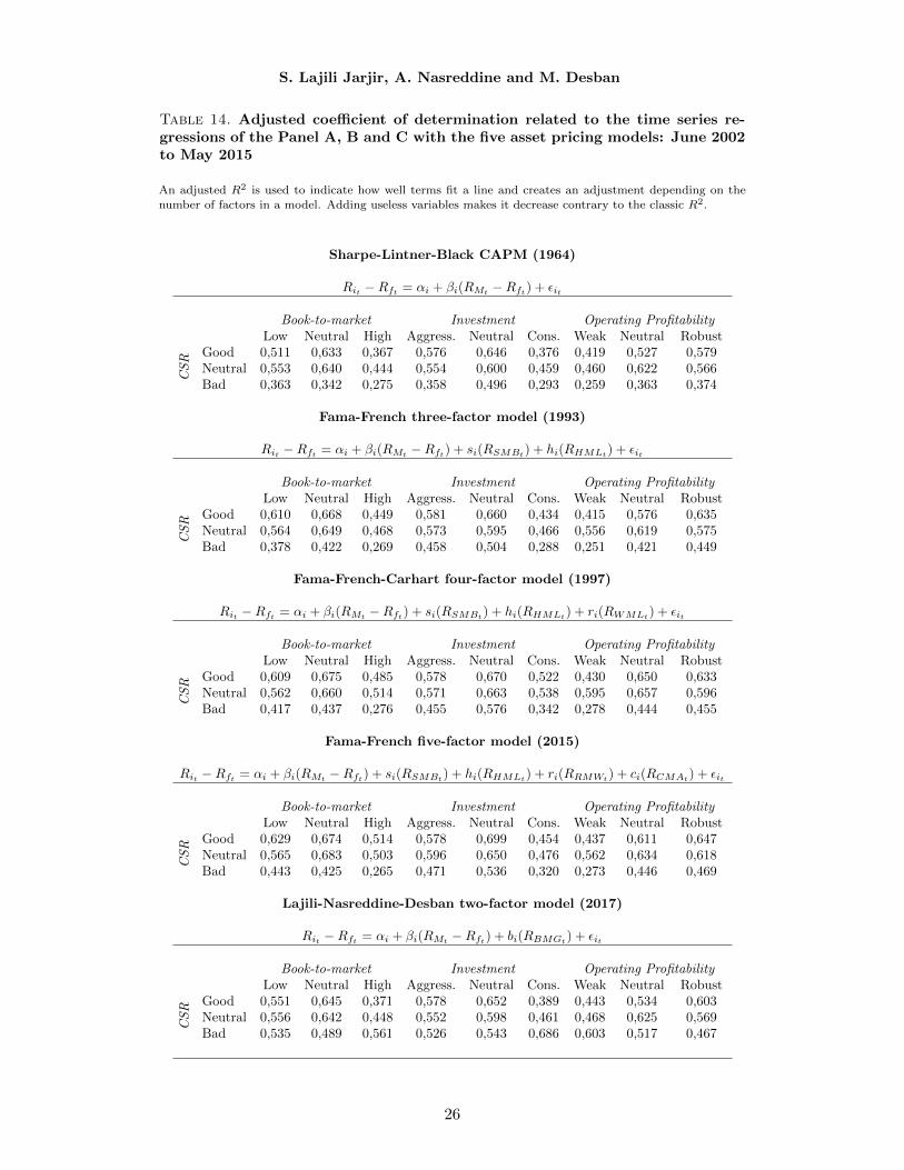
S. Lajili Jarjir, A. Nasreddine and M. Desban
Table 14. Adjusted coefficient of determination related to the time series re-gressions of the Panel A, B and C with the five asset pricing models: June 2002to May 2015
An adjusted R2 is used to indicate how well terms fit a line and creates an adjustment depending on the
number of factors in a model. Adding useless variables makes it decrease contrary to the classic R2.
Sharpe-Lintner-Black CAPM (1964)
Rit −Rft = αi + βi(RMt −Rft) + εit
Book-to-market Investment Operating ProfitabilityLow Neutral High Aggress. Neutral Cons. Weak Neutral Robust
CS
R
Good 0,511 0,633 0,367 0,576 0,646 0,376 0,419 0,527 0,579Neutral 0,553 0,640 0,444 0,554 0,600 0,459 0,460 0,622 0,566Bad 0,363 0,342 0,275 0,358 0,496 0,293 0,259 0,363 0,374
Fama-French three-factor model (1993)
Rit −Rft = αi + βi(RMt−Rft) + si(RSMBt) + hi(RHMLt) + εit
Book-to-market Investment Operating ProfitabilityLow Neutral High Aggress. Neutral Cons. Weak Neutral Robust
CS
R
Good 0,610 0,668 0,449 0,581 0,660 0,434 0,415 0,576 0,635Neutral 0,564 0,649 0,468 0,573 0,595 0,466 0,556 0,619 0,575Bad 0,378 0,422 0,269 0,458 0,504 0,288 0,251 0,421 0,449
Fama-French-Carhart four-factor model (1997)
Rit −Rft = αi + βi(RMt−Rft) + si(RSMBt) + hi(RHMLt) + ri(RWMLt) + εit
Book-to-market Investment Operating ProfitabilityLow Neutral High Aggress. Neutral Cons. Weak Neutral Robust
CS
R
Good 0,609 0,675 0,485 0,578 0,670 0,522 0,430 0,650 0,633Neutral 0,562 0,660 0,514 0,571 0,663 0,538 0,595 0,657 0,596Bad 0,417 0,437 0,276 0,455 0,576 0,342 0,278 0,444 0,455
Fama-French five-factor model (2015)
Rit −Rft = αi + βi(RMt−Rft) + si(RSMBt) + hi(RHMLt) + ri(RRMWt
) + ci(RCMAt) + εit
Book-to-market Investment Operating ProfitabilityLow Neutral High Aggress. Neutral Cons. Weak Neutral Robust
CS
R
Good 0,629 0,674 0,514 0,578 0,699 0,454 0,437 0,611 0,647Neutral 0,565 0,683 0,503 0,596 0,650 0,476 0,562 0,634 0,618Bad 0,443 0,425 0,265 0,471 0,536 0,320 0,273 0,446 0,469
Lajili-Nasreddine-Desban two-factor model (2017)
Rit −Rft = αi + βi(RMt−Rft) + bi(RBMGt) + εit
Book-to-market Investment Operating ProfitabilityLow Neutral High Aggress. Neutral Cons. Weak Neutral Robust
CS
R
Good 0,551 0,645 0,371 0,578 0,652 0,389 0,443 0,534 0,603Neutral 0,556 0,642 0,448 0,552 0,598 0,461 0,468 0,625 0,569Bad 0,535 0,489 0,561 0,526 0,543 0,686 0,603 0,517 0,467
26