a comparison of heuristic algorithms for custom
TRANSCRIPT
HAL Id: hal-01354991https://hal.inria.fr/hal-01354991
Submitted on 24 Oct 2016
HAL is a multi-disciplinary open accessarchive for the deposit and dissemination of sci-entific research documents, whether they are pub-lished or not. The documents may come fromteaching and research institutions in France orabroad, or from public or private research centers.
L’archive ouverte pluridisciplinaire HAL, estdestinée au dépôt et à la diffusion de documentsscientifiques de niveau recherche, publiés ou non,émanant des établissements d’enseignement et derecherche français ou étrangers, des laboratoirespublics ou privés.
Distributed under a Creative Commons Attribution - NoDerivatives| 4.0 InternationalLicense
A comparison of heuristic algorithms for custominstruction selection
Shanshan Wang, Chenglong Xiao, Wanjun Liu, Emmanuel Casseau
To cite this version:Shanshan Wang, Chenglong Xiao, Wanjun Liu, Emmanuel Casseau. A comparison of heuristic al-gorithms for custom instruction selection. Microprocessors and Microsystems: Embedded HardwareDesign (MICPRO), Elsevier, 2016, 45 (A), pp.176-186. �10.1016/j.micpro.2016.05.001�. �hal-01354991�
A Comparison of Heuristic Algorithms for Custom Instructio n Selection
Shanshan Wang∗, Chenglong Xiao∗,Wanjun Liu∗,Emmanuel Casseau†
∗Liaoning Technical University, China{celine.shanshan.wang,chenglong.xiao}@gmail.com
[email protected]†University of Rennes I, Inria, France
Abstract—Extensible processors with custom function units(CFU) that implement parts of the application code can makegood trade-off between performance and flexibility. In general,deciding profitable parts of the application source code thatrun on CFU involves two crucial steps: subgraph enumerationand subgraph selection. In this paper, we focus on the subgraphselection problem, which has been widely recognized as acomputationally difficult problem. We have formally provedthat the upper bound of the number of feasible solutions forthe subgraph selection problem is3n/3, wheren is the numberof subgraph candidates. We have adapted and comparedfive popular heuristic algorithms: simulated annealing (SA),tabu search (TS), genetic algorithm (GA), particle swarmoptimization (PSO) and ant colony optimization (ACO), for thesubgraph selection problem with the objective of minimisingexecution time under non-overlapping constraint and acyclicityconstraint. The results show that the standard SA algorithmcan produce the best results while taking the least amount oftime among the five standard heuristics. In addition, we haveintroduced an adaptive local optimum searching strategy inACO and PSO to further improve the quality of results.
Keywords-Heuristic algorithms; Data-flow graph; Extensibleprocessors; Custom instructions; Custom function units;
I. I NTRODUCTION
Due to a good trade-offs between performance and flex-ibility, extensible processors have been used more andmore in embedded systems. Such examples include AlteraNIOS processors, Xilinx MicroBlaze and ARC processors.In extensible processors, a base processor is extended withcustom function units that execute custom instructions.Custom function units running the computation-intensiveparts of application can be implemented with application-specific integrated-circuit or field-programmable gate-arraytechnology. A custom instruction is composed of a clusterof primitive instructions. In general, the critical parts of anapplication are selected to execute on CFUs and the rest partsare run on the base processor. With the base processor, theflexibility can be guaranteed. As selected custom instructionsusually impose high data-level parallelism [1], executingthese custom instructions on CFUs may significantly im-prove the performance.
Deciding which segments of code to be executed in CFUsis a time-consuming work. Due to time-to-market pressure
and requirement for lower design cost of extensible proces-sors, automated custom instruction generation is necessary.Fig 1. shows the design flow for automatic custom instruc-tion generation. Starting with provided C/C++ code, a front-end compiler is called to produce the corresponding controldata-flow graph (CDFG). Then, the subgraph enumerationstep enumerates all subgraphs (graphic representation of cus-tom instructions) from DFGs inside CDFG that satisfy themicro-architecture constraints and user-defined constraints[2]–[5]. Next, in order to improve the performance, thesubgraph selection step selects a subset of most profitablesubgraphs from the set of enumerated subgraphs, whilesatisfying some constraints (e.g. non-overlapping constraintand area constraint). Based on the selected subgraphs, thesubgraphs with equivalent structure and function are groupedtogether. The behavioral descriptions of the selected custominstructions along with the code incorporating the selectedcustom instructions are finally produced. The crucial prob-lems involved in custom instruction generation are: subgraphenumeration and subgraph selection. In this paper, we focuson the subgraph selection problem. The main contributionsof this paper are:• formulating the subgraph selection problem as a maxi-
mum cliques problem;• an upper bound on the number of feasible solutions is
3n/3, wheren is the number of subgraph candidates;• adaptation of five popular heuristic algorithms for the
subgraph selection problem;• detailed comparison of these five algorithms in terms
of search time and quality of the solutions. Furthermore, weextend PSO and ACO algorithms to include an adaptive localoptimum searching strategy. Results show that the quality ofthe solutions can be further improved.
The rest of the paper is organized as follows. Section 2reviews the related work on the subgraph selection problem,while section 3 formally formulates the subgraph selectionproblem as a weighted maximum problem and presents anupper bound on the number of feasible solutions. Section4 discusses the proposed SA, TS, GA, PSO and ACOalgorithms for the subgraph selection problem. In section5, the experiments with practical benchmarks are performedto evaluate the algorithms in terms of search time and quality

Front-end
Subgraph
Enumeration
Subgraph
Selection
Code
Generation
Architectural
Constraints
Design Objective
Application Code
Optimized Code
Estimated
Latency&Area
Figure 1. The design flow for custom instruction generation
of the solutions. Some discussion on the future work is givenin section 6. Section 7 concludes this paper.
II. RELATED WORK
Prior to review the related work on custom instructionselection (or subgraph selection), we start by discussingalgorithms for custom instruction enumeration.
Plenty of previous research on custom instruction enu-meration have been presented in recent years. The cus-tom instruction enumeration tries to enumerate a set ofsubgraphs from the application graph with respect to themicro-architecture constraints or user-defined constraints.The custom instruction enumeration process is usually verytime-consuming. For example, it was proven in [6] that thenumber of valid subgraphs satisfying the convexity and I/Oconstraints isnI+O, wheren is the number of nodes in theapplication graph, andI andO are the maximum numberof inputs and outputs respectively. A set of algorithmswith O(nI+O) time complexity can be found in existingliterature [3], [5], [7]. Some other algorithms targeted toonly enumerate maximal convex subgraphs by relaxing theI/O constraints have also been proposed [8], [9]. However,the number of maximal convex subgraphs can still be expo-nential. In [10], the number of maximal convex subgraphswas formally proven to be2|F |, where F is the set offorbidden nodes in the application graph. It can be observedfrom previous experiments that the subgraph enumerationstep may produce tens of thousands of subgraphs for bothenumeration of convex subgraphs under I/O constraints andenumeration of maximal convex subgraphs.
Subgraph selectionis the process of selecting a subset ofprofitable subgraphs from the set of enumerated subgraphsas custom instructions that will be implemented in custom
function units. As the number of candidate subgraphs canbe very large, the subgraph selection problem is generallyconsidered as a computationally difficult problem [1]. Pre-vious work on subgraph selection problem can be groupedinto two categories:
Optimal algorithms: Some of previous work try to findexact solution for the subgraph selection problem. Forexample, the authors of [11] propose a branch-and-boundalgorithm for selecting the optimal subset of custom instruc-tions. Cong et al. solve this problem by using dynamic pro-gramming [12]. Some other researchers address the subgraphselection problem using integer linear programming (ILP)or linear programming (LP) [13]–[15]. These methods treatthe selection problem as maximizing or minimizing a linearobjective function, while each subgraph is represented as avariable, which has a boolean value. The area constraint ornon-overlapping constraint is expressed as linear inequality.These formulations are provided to an ILP or LP solveras input. Then, the solver may produce a solution. Similarto LP method, Martin et al. try to deal with the selectionproblem by using constraint programming method [16], [17].However, due to the complexity of the subgraph selectionproblem, these methods may fail to produce a solution whenthe size of the application graph becomes large.
Although the subgraph selection problem is widely con-sidered as a computationally difficult problem, it still lacksof an exact upper bound on the number of feasible solutions.In this article, we first formulate the subgraph selectionproblem under non-overlapping constraint as a maximumclique problem. Then, with this formulation, the upper boundon the number of feasible solutions is formally proved to be3n/3, wheren is the number of subgraphs.
Heuristic algorithms: Since optimal algorithms are usuallyintractable when the problem size is large, it is necessaryto solve the problem with heuristic algorithms. Kastner etal. heuristically solve the problem by contracting the mostfrequently occurring edges [18]. Wolinski and Kunchcinskipropose a method that selects candidates based on theoccurrence of specific nodes [19]. A method attempting topreferentially select the subgraphs along the longest pathofa given application graph has been proposed by Clark et al[20].
In recent years, due to good scalability and trade-offsbetween search time and quality of the solutions, manymeta-heuristic algorithms have been proposed to solve thesubgraph selection problem. As an example, a genetic algo-rithm (GA) is introduced to overcome the intractability of thesubgraph selection problem [3]. The experiments show thatthe genetic algorithm may produce near-optimal solutionsfor problems with different sizes. In [21], a tabu searchalgorithm (TS) is adapted to solve the subgraph selectionproblem. The authors report that the tabu search algorithmcan provide optimal solutions for medium-sized problems.It can still produce solutions when optimal algorithms fail
to produce solutions for large-sized problems. Other meta-heuristic algorithms like particle swarm optimization (PSO)[22], ant colony optimization (ACO) [23], [24] and simulat-ed annealing algorithms (SA) [25] have been also introducedor adapted to address the subgraph selection problem orsimilar problems. However, the comparisons between thesepopular meta-heuristic algorithms are still missing in theexisting literature. Thus, the main objective of this paperis to adapt the SA, TS, GA, PSO and ACO algorithms tosolve the subgraph selection problem, and compare thesealgorithms in terms of runtime and quality of the results.
III. PROBLEM FORMULATION
The definition of the subgraph selection problem dis-cussed in this paper is based on the following notations.
Each basic block in an application can be representedas a directed acyclic graphG = (V,E), where V ={v1, v2, ..., vm} represents the primitive instructions andEindicates the data dependency between instructions. A cus-tom instruction can be graphically expressed as a subgraphSi = {Vi, Ei} of G (Vi ⊆ V andEi ⊆ E).
Similar to [26], every nodevi in Si is associated with asoftware latencysi. The accumulated software latencyLi ofeach subgraph can be calculated as follows:
Li =∑
vi∈Si
si (1)
Each subgraph candidate is associated with a performancegain Pi. The performance gain represents the number ofclock cycles saved by executing the set of primitive instruc-tions in a custom function unit instead of executing them inthe base processor. The calculation for the performance gainof each subgraph is as follows:
Pi = Li − (HWi + Ei) (2)
where HWi indicates the latency of executing theseprimitive instructions in the corresponding custom functionunit, andEi represents the extra time required to transfer theinput and output operands of the custom instruction from andto the core register files.
Definition 1. Non-overlapping constraint: The subgraphsenumerated by the subgraph enumeration step mayhave some nodes in common (overlapping). Althoughallowing overlapping between selected subgraphs maybring better performance improvement, it may make thecode regeneration intractable and increase unnecessarypower consumption. Similar to most existing work [21],[26], [27], we apply the non-overlapping constraint for theselection problem in this paper.
Definition 2. Acyclicity constraint: Two enumerated sub-graphs may provide data to each other. If these two sub-graphs are selected together, then a cycle is formed. This
2
3
4
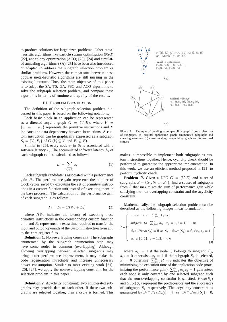
1
Figure 2. Example of building a compatibility graph from a given setof subgraphs. (a) original application graph, enumerated subgraphs andcovering solutions. (b) corresponding compatibility graph and its maximalcliques
makes it impossible to implement both subgraphs as cus-tom instructions together. Hence, cyclicity check should beperformed to guarantee the appropriate implementation. Inthis work, we use an efficient method proposed in [21] toperform cyclicity check.
Problem P . Given a DFGG = (V,E) and a set ofsubgraphsS = {S1, S2, ..., Sn}, find a subset of subgraphsfrom S that maximizes the sum of performance gain whilesatisfying the non-overlapping constraint and the acyclicityconstraint.
Mathematically, the subgraph selection problem can bedescribed as the following integer linear formulation:
P =
maximize∑n
i=1Pi · xi
subject to∑n
j=1aij · xj = 1, i = 1, · · ·, m
Si ∩ Pred(Sj) = ∅ or Si ∩ Succ(Sj) = ∅, ∀xi, xj = 1
xi ∈ {0, 1}, i = 1, 2, · · ·, n
(3)
whereaij = 1 if the nodevi belongs to subgraphSj ,aij = 0 otherwise.xi = 1 if the subgraphSi is selected,xi = 0 otherwise.
∑ni=1 Pi · xi indicates the objective of
minimising the execution time of the application code (max-imizing the performance gain).
∑nj=1 aijxj = 1 guarantees
each node is only covered by one selected subgraph suchthat the non-overlapping constraint is satisfied.Pred(Sj)andSucc(Sj) represent the predecessors and the successorsof subgraphSj respectively. The acyclicity constraint isguaranteed bySi ∩ Pred(Sj) = ∅ or Si ∩ Succ(Sj) = ∅.
Definition 3. A feasible solution to the subgraph selectionproblem is a solution which satisfies all its constraints. Anoptimal solution to the subgraph selection problem is afeasible solution which maximizes its objective function.
Definition 4. Two subgraphs in a feasible solution are saidto be compatible if and only if two subgraphs satisfying bothnon-overlapping constraint and acyclicity constraint.
Definition 5. The compatibility graphC(S) of a set ofsubgraphsS = {S1, S2, ..., Sn} is an undirected graphwhose nodes correspond to the subgraphs inS, and an edgeis placed between two nodes corresponding to subgraphsSi
andSj if and only if Si andSj are compatible. It is clear thatany two nodes have no edge between them if they overlap(Si ∩ Sj 6= ∅) or if there exists a cycle between them. Fig.2 shows an example of building the compatibility graph fora given set of subgraphs.
Theorem 1: Each feasible solution corresponds to a max-imal clique in the compatibility graph and vice versa.
Proof: Assume that a feasible solution is composed ofsubgraphsS1, · · ·, Sp. Since the solution is feasible, any twosubgraphsSi andSj in the solution are compatible. Thenthere must be an edge betweenSi andSj in the compatibilitygraph, soS1, · · ·, Sp is a clique.
On the other hand, suppose thatS1, · · ·, Sp is a maximalclique in the compatibility graph, and that the correspondingsolution cannot fully cover the original application graphG.Assume a nodev of G is not covered by any of the subgraphsin the maximal clique. Then a subgraphSk containing onlythe nodev is not in the maximal clique. As the subgraphSk is connected to each subgraph inS1, · · ·, Sp, thus,S1, · ··, Sp, Sk is a clique, contradicting the assumption that theformer clique is maximal. Therefore, a maximal clique inthe compatibility graph corresponds to a feasible solution.
Theorem 2: There exists an upper bound of3n/3 onthe number of feasible solutions for the subgraph selectionproblemP .
Proof: By applying Theorem 1, the number of feasiblesolutions for P should be the same as the number ofmaximal cliques in the compatibility graph. As we knownthat the number of maximal cliques in a graph withnnodes is bounded by3n/3 [28], thus, the number of feasiblesolutions forP is bounded by3n/3.
With Theorem 1, we known that each feasible solutioncorresponds to a maximal clique in the compatibility graph.It is not difficult to understand that an optimal solution ofthe problemP corresponds to a maximum clique among allthe maximal cliques. Therefore, the problemP can be alsoviewed as a typical weighted maximum clique problem.
IV. H EURISTIC OPTIMIZATION ALGORITHMS
This section presents how the five heuristic algorithmsare adapted to solve the problemP . An adaptive strategy
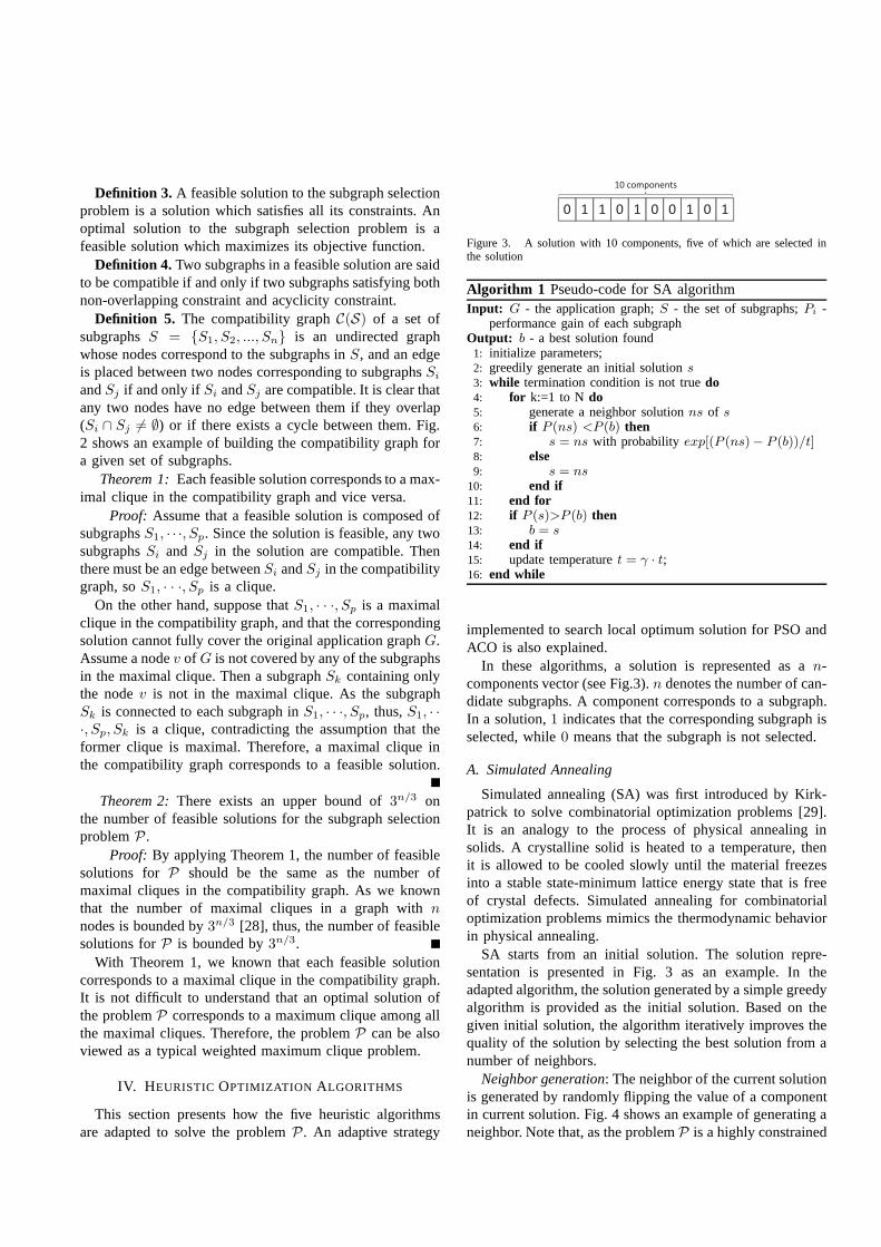
00 11 11 00 11 00 00 11 00 11
10 components
Figure 3. A solution with 10 components, five of which are selected inthe solution
Algorithm 1 Pseudo-code for SA algorithmInput: G - the application graph;S - the set of subgraphs;Pi -
performance gain of each subgraphOutput: b - a best solution found
1: initialize parameters;2: greedily generate an initial solutions3: while termination condition is not truedo4: for k:=1 to N do5: generate a neighbor solutionns of s6: if P (ns) <P (b) then7: s = ns with probability exp[(P (ns)− P (b))/t]8: else9: s = ns
10: end if11: end for12: if P (s)>P (b) then13: b = s14: end if15: update temperaturet = γ · t;16: end while
implemented to search local optimum solution for PSO andACO is also explained.
In these algorithms, a solution is represented as an-components vector (see Fig.3).n denotes the number of can-didate subgraphs. A component corresponds to a subgraph.In a solution,1 indicates that the corresponding subgraph isselected, while0 means that the subgraph is not selected.
A. Simulated Annealing
Simulated annealing (SA) was first introduced by Kirk-patrick to solve combinatorial optimization problems [29].It is an analogy to the process of physical annealing insolids. A crystalline solid is heated to a temperature, thenit is allowed to be cooled slowly until the material freezesinto a stable state-minimum lattice energy state that is freeof crystal defects. Simulated annealing for combinatorialoptimization problems mimics the thermodynamic behaviorin physical annealing.
SA starts from an initial solution. The solution repre-sentation is presented in Fig. 3 as an example. In theadapted algorithm, the solution generated by a simple greedyalgorithm is provided as the initial solution. Based on thegiven initial solution, the algorithm iteratively improves thequality of the solution by selecting the best solution from anumber of neighbors.
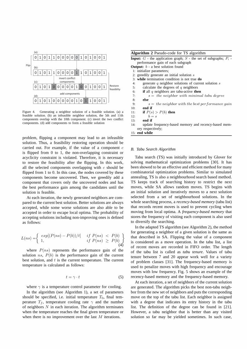
Neighbor generation: The neighbor of the current solutionis generated by randomly flipping the value of a componentin current solution. Fig. 4 shows an example of generating aneighbor. Note that, as the problemP is a highly constrained
00 11 00 11 11 00 00 00 00 0 11 00 11 00 00 11
00 11 00 11 11 00 00 00 00 1 11 00 11 00 00 11
00 11 00 11 0 00 00 0 00 11 00 11 00 00 11
00 11 00 11 00 00 00 00 00 11 00 1 11 00 00 11
0
invert conflict
components
add components
(a):
(b):
(c):
(d):
Restore
feasiblity
Flip
Figure 4. Generating a neighbor solution of a feasible solution. (a) afeasible solution. (b) an infeasible neighbor solution, the 5th and 11thcomponents overlap with the 10th component. (c) invert the two conflictcomponents. (d) add components to form a feasible solution
problem, flipping a component may lead to an infeasiblesolution. Thus, a feasibility restoring operation should becarried out. For example, if the value of a componentcis flipped from 0 to 1, the non-overlapping constraint oracyclicity constraint is violated. Therefore, it is necessaryto restore the feasibility after the flipping. In this work,all the selected components overlapping withc should beflipped from 1 to 0. In this case, the nodes covered by thesecomponents become uncovered. Then, we greedily add acomponent that covers only the uncovered nodes and hasthe best performance gain among the candidates until thesolution is feasible.
At each iteration, the newly generated neighbors are com-pared to the current best solution. Better solutions are alwaysaccepted, while some worse solutions are also able to beaccepted in order to escape local optima. The probability ofaccepting solutions including non-improving ones is definedas follows:
L(ns) =
{
exp[(P (ns)− P (b))/t] if P (ns) < P (b)1, if P (ns) ≥ P (b)
}
(4)where P (ns) represents the performance gain of the
solution ns, P (b) is the performance gain of the currentbest solution, andt is the current temperature. The currenttemperature is calculated as follows:
t = γ · t (5)
whereγ is a temperature control parameter for cooling.In the algorithm (see Algorithm 1), a set of parameters
should be specified, i.e. initial temperatureT0, final tem-peratureTf , temperature cooling rateγ and the numberof neighborsN in each iteration. The algorithm terminateswhen the temperature reaches the final given temperature orwhen there is no improvement over the lastM iterations.
Algorithm 2 Pseudo-code for TS algorithmInput: G - the application graph;S - the set of subgraphs;Pi -
performance gain of each subgraphOutput: b - a best solution found
1: initialize parameters;2: greedily generate an initial solutions3: while termination condition is not truedo4: generateq neighbor solutions of current solutions5: calculate the degrees ofq neighbors6: if all q neighbors are tabu-activethen7: s = the neighbor with minimal tabu degree8: else9: s = the neighbor with the best performance gain
10: end if11: if P (s) > P (b) then12: b = s13: end if14: update frequency-based memory and recency-based mem-
ory respectively;15: end while
B. Tabu Search Algorithm
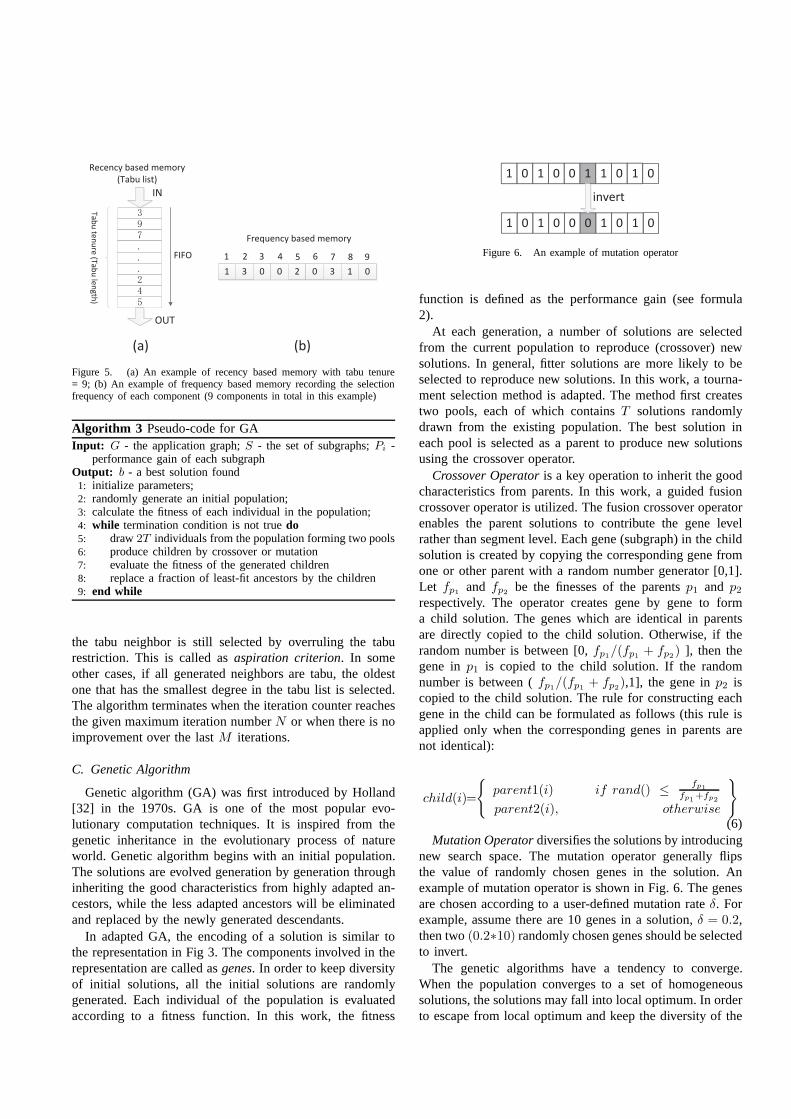
Tabu search (TS) was initially introduced by Glover forsolving mathematical optimization problems [30]. It hasbeen showed to be an effective and efficient method for manycombinatorial optimization problems. Similar to simulatedannealing, TS is also a neighbourhood search based method.TS keeps track of searching history to restrict the nextmoves, while SA allows random moves. TS begins withan initial solution and iteratively moves to a next solutionselected from a set of neighbourhood solutions. In thewhole searching process, arecency-based memory (tabu list)that records recent moves is used to prevent cycling whenmoving from local optima. Afrequency-based memory thatstores the frequency of visiting each component is also usedto diversify the searching.
In the adapted TS algorithm (see Algorithm 2), the methodfor generating a neighbor of a given solution is the same asthat described in SA. Flipping the value of a componentis considered as a move operation. In the tabu list, a listof recent moves are recorded in FIFO order. The lengthof the tabu list is called astabu tenure. Values of tabutenure between 7 and 20 appear work well for a varietyof problem classes [31]. The frequency-based memory isused to penalize moves with high frequency and encouragemoves with low frequency. Fig. 5 shows an example of therecency-based memory and the frequency-based memory.
At each iteration, a set of neighbors of the current solutionare generated. The algorithm picks the best non-tabu neigh-bor from the new set of neighbors and puts the correspondingmove on the top of the tabu list. Each neighbor is assignedwith a degree that indicates its entry history in the tabulist. The definition of the degree can be found in [21].However, a tabu neighbor that is better than any visitedsolution so far may be yielded sometimes. In such case,
Recency based memory
(Tabu list)
Ta
bu
ten
ure
(Ta
bu
len
gth
)
IN
OUT
FIFO
1 3 0 0 2 0 3 1 0
Frequency based memory
1 2 3 4 5 6 7 8 9
(a) (b)
Figure 5. (a) An example of recency based memory with tabu tenure= 9; (b) An example of frequency based memory recording the selectionfrequency of each component (9 components in total in this example)
Algorithm 3 Pseudo-code for GAInput: G - the application graph;S - the set of subgraphs;Pi -
performance gain of each subgraphOutput: b - a best solution found
1: initialize parameters;2: randomly generate an initial population;3: calculate the fitness of each individual in the population;4: while termination condition is not truedo5: draw2T individuals from the population forming two pools6: produce children by crossover or mutation7: evaluate the fitness of the generated children8: replace a fraction of least-fit ancestors by the children9: end while
the tabu neighbor is still selected by overruling the taburestriction. This is called asaspiration criterion. In someother cases, if all generated neighbors are tabu, the oldestone that has the smallest degree in the tabu list is selected.The algorithm terminates when the iteration counter reachesthe given maximum iteration numberN or when there is noimprovement over the lastM iterations.
C. Genetic Algorithm
Genetic algorithm (GA) was first introduced by Holland[32] in the 1970s. GA is one of the most popular evo-lutionary computation techniques. It is inspired from thegenetic inheritance in the evolutionary process of natureworld. Genetic algorithm begins with an initial population.The solutions are evolved generation by generation throughinheriting the good characteristics from highly adapted an-cestors, while the less adapted ancestors will be eliminatedand replaced by the newly generated descendants.
In adapted GA, the encoding of a solution is similar tothe representation in Fig 3. The components involved in therepresentation are called asgenes. In order to keep diversityof initial solutions, all the initial solutions are randomlygenerated. Each individual of the population is evaluatedaccording to a fitness function. In this work, the fitness
11 00 11 00 00 1 11 00 11 00
11 00 11 00 00 0 11 00 11 00
invert
Figure 6. An example of mutation operator
function is defined as the performance gain (see formula2).
At each generation, a number of solutions are selectedfrom the current population to reproduce (crossover) newsolutions. In general, fitter solutions are more likely to beselected to reproduce new solutions. In this work, a tourna-ment selection method is adapted. The method first createstwo pools, each of which containsT solutions randomlydrawn from the existing population. The best solution ineach pool is selected as a parent to produce new solutionsusing the crossover operator.
Crossover Operator is a key operation to inherit the goodcharacteristics from parents. In this work, a guided fusioncrossover operator is utilized. The fusion crossover operatorenables the parent solutions to contribute the gene levelrather than segment level. Each gene (subgraph) in the childsolution is created by copying the corresponding gene fromone or other parent with a random number generator [0,1].Let fp1 and fp2 be the finesses of the parentsp1 and p2respectively. The operator creates gene by gene to forma child solution. The genes which are identical in parentsare directly copied to the child solution. Otherwise, if therandom number is between [0,fp1/(fp1 + fp2) ], then thegene inp1 is copied to the child solution. If the randomnumber is between (fp1/(fp1 + fp2),1], the gene inp2 iscopied to the child solution. The rule for constructing eachgene in the child can be formulated as follows (this rule isapplied only when the corresponding genes in parents arenot identical):
child(i)=
{
parent1(i) if rand() ≤fp1
fp1+fp2parent2(i), otherwise
}
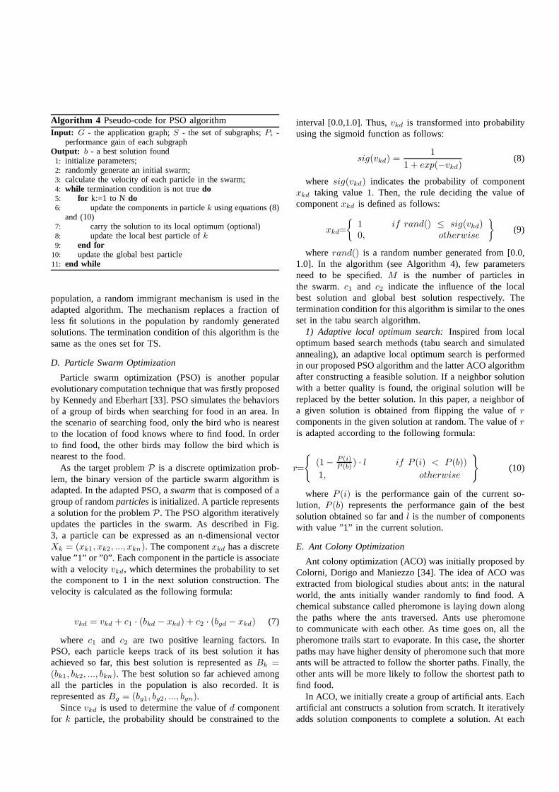
(6)Mutation Operator diversifies the solutions by introducing
new search space. The mutation operator generally flipsthe value of randomly chosen genes in the solution. Anexample of mutation operator is shown in Fig. 6. The genesare chosen according to a user-defined mutation rateδ. Forexample, assume there are 10 genes in a solution,δ = 0.2,then two(0.2∗10) randomly chosen genes should be selectedto invert.
The genetic algorithms have a tendency to converge.When the population converges to a set of homogeneoussolutions, the solutions may fall into local optimum. In orderto escape from local optimum and keep the diversity of the
Algorithm 4 Pseudo-code for PSO algorithmInput: G - the application graph;S - the set of subgraphs;Pi -
performance gain of each subgraphOutput: b - a best solution found
1: initialize parameters;2: randomly generate an initial swarm;3: calculate the velocity of each particle in the swarm;4: while termination condition is not truedo5: for k:=1 to N do6: update the components in particlek using equations (8)
and (10)7: carry the solution to its local optimum (optional)8: update the local best particle ofk9: end for
10: update the global best particle11: end while
population, a random immigrant mechanism is used in theadapted algorithm. The mechanism replaces a fraction ofless fit solutions in the population by randomly generatedsolutions. The termination condition of this algorithm is thesame as the ones set for TS.
D. Particle Swarm Optimization
Particle swarm optimization (PSO) is another popularevolutionary computation technique that was firstly proposedby Kennedy and Eberhart [33]. PSO simulates the behaviorsof a group of birds when searching for food in an area. Inthe scenario of searching food, only the bird who is nearestto the location of food knows where to find food. In orderto find food, the other birds may follow the bird which isnearest to the food.
As the target problemP is a discrete optimization prob-lem, the binary version of the particle swarm algorithm isadapted. In the adapted PSO, aswarm that is composed of agroup of randomparticles is initialized. A particle representsa solution for the problemP . The PSO algorithm iterativelyupdates the particles in the swarm. As described in Fig.3, a particle can be expressed as an n-dimensional vectorXk = (xk1, xk2, ..., xkn). The componentxkd has a discretevalue ”1” or ”0”. Each component in the particle is associatewith a velocityvkd, which determines the probability to setthe component to 1 in the next solution construction. Thevelocity is calculated as the following formula:
vkd = vkd + c1 · (bkd − xkd) + c2 · (bgd − xkd) (7)
where c1 and c2 are two positive learning factors. InPSO, each particle keeps track of its best solution it hasachieved so far, this best solution is represented asBk =(bk1, bk2, ..., bkn). The best solution so far achieved amongall the particles in the population is also recorded. It isrepresented asBg = (bg1, bg2, ..., bgn).
Sincevkd is used to determine the value ofd componentfor k particle, the probability should be constrained to the
interval [0.0,1.0]. Thus,vkd is transformed into probabilityusing the sigmoid function as follows:
sig(vkd) =1
1 + exp(−vkd)(8)
where sig(vkd) indicates the probability of componentxkd taking value 1. Then, the rule deciding the value ofcomponentxkd is defined as follows:
xkd=
{
1 if rand() ≤ sig(vkd)0, otherwise
}
(9)
whererand() is a random number generated from [0.0,1.0]. In the algorithm (see Algorithm 4), few parametersneed to be specified.M is the number of particles inthe swarm.c1 and c2 indicate the influence of the localbest solution and global best solution respectively. Thetermination condition for this algorithm is similar to the onesset in the tabu search algorithm.
1) Adaptive local optimum search: Inspired from localoptimum based search methods (tabu search and simulatedannealing), an adaptive local optimum search is performedin our proposed PSO algorithm and the latter ACO algorithmafter constructing a feasible solution. If a neighbor solutionwith a better quality is found, the original solution will bereplaced by the better solution. In this paper, a neighbor ofa given solution is obtained from flipping the value ofrcomponents in the given solution at random. The value ofris adapted according to the following formula:
r=
{
(1− P (i)P (b) ) · l if P (i) < P (b))
1, otherwise
}
(10)
whereP (i) is the performance gain of the current so-lution, P (b) represents the performance gain of the bestsolution obtained so far andl is the number of componentswith value ”1” in the current solution.
E. Ant Colony Optimization
Ant colony optimization (ACO) was initially proposed byColorni, Dorigo and Maniezzo [34]. The idea of ACO wasextracted from biological studies about ants: in the naturalworld, the ants initially wander randomly to find food. Achemical substance called pheromone is laying down alongthe paths where the ants traversed. Ants use pheromoneto communicate with each other. As time goes on, all thepheromone trails start to evaporate. In this case, the shorterpaths may have higher density of pheromone such that moreants will be attracted to follow the shorter paths. Finally,theother ants will be more likely to follow the shortest path tofind food.
In ACO, we initially create a group of artificial ants. Eachartificial ant constructs a solution from scratch. It iterativelyadds solution components to complete a solution. At each
Algorithm 5 Pseudo-code for ACO algorithmInput: G - the application graph;S - the set of subgraphs;Pi -
performance gain of each subgraphOutput: b - a best solution found
1: initialize parameters;2: while termination condition is not truedo3: for k:=1 to N do4: while solution not completeddo5: computeη(c), Pk(c)6: select the component to add, with probabilityPk(c)7: end while8: carry the solution to its local optimum (optional)9: end for
10: update pheromone trailsτi(c) = ρ · τi−1(c) +∑N
k=1△τk(c);
11: end while
iteration, the ant selects a solution component according toa probabilistic state transition rule. The probabilistic statetransition rule gives the probability that a componentc isselected by antk:
Pk(c)=
{
α·τ(c)+β·η(c)∑υ∈Uk(c)(α·τ(υ)+β·η(υ)) if c ∈ Uk(c)
0, otherwise
}
(11)whereτ(c) is the pheromone trail on componentc, η(c)
is a local heuristic information for rewarding the componentleading to good performance gain.α andβ are parametersthat allow a user to control the relative importance of thepheromone trail versus performance gain.Uk(c) is the setof components that remain to be visited by antk positionedon componentc.
The heuristic informationη(c) is implemented as follows:
η(c) =Pc
ms(12)
wherePc is the performance gain obtained by componentc, ms is the maximum performance gain obtained by acomponent among all the components.
After ant k completes a solution, a global update shouldbe performed to calculate the pheromone trail taking intoaccount evaporation and increment:
τi(c) = ρ · τi−1(c) +
N∑
k=1
△τk(c) (13)
where0 < ρ < 1 andρ is a coefficient which representsthe extent the pheromone retained on the componentc. N isthe number of ants.△τk(c) is the pheromone antk depositson the componentc. △τk(c) is calculated as follows:
△τk(c)=
{
1− 1P (k)+1 if c is selected by ant k
0, otherwise
}
(14)
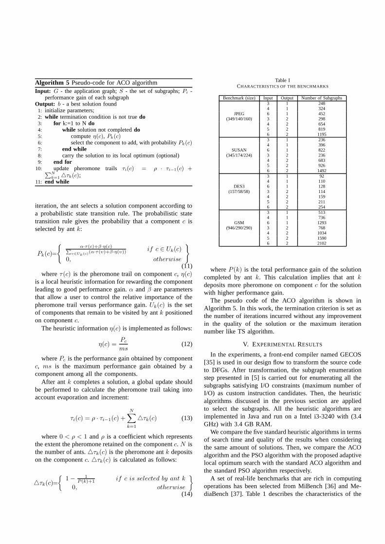
Table ICHARACTERISTICS OF THE BENCHMARKS
Benchmark (size) Input Output Number of Subgraphs3 1 2484 1 324
JPEG 6 1 452(349/140/160) 3 2 298
4 2 6545 2 8196 2 11953 1 2364 1 396
SUSAN 6 1 822(345/174/224) 3 2 236
4 2 6835 2 9266 2 14923 1 924 1 110
DES3 6 1 128(157/58/58) 3 2 114
4 2 1595 2 2116 2 2543 1 5134 1 736
GSM 6 1 1293(946/290/290) 3 2 768
4 2 10345 2 15906 2 2102
whereP (k) is the total performance gain of the solutioncompleted by antk. This calculation implies that antkdeposits more pheromone on componentc for the solutionwith higher performance gain.
The pseudo code of the ACO algorithm is shown inAlgorithm 5. In this work, the termination criterion is set asthe number of iterations incurred without any improvementin the quality of the solution or the maximum iterationnumber like TS algorithm.
V. EXPERIMENTAL RESULTS
In the experiments, a front-end compiler named GECOS[35] is used in our design flow to transform the source codeto DFGs. After transformation, the subgraph enumerationstep presented in [5] is carried out for enumerating all thesubgraphs satisfying I/O constraints (maximum number ofI/O) as custom instruction candidates. Then, the heuristicalgorithms discussed in the previous section are appliedto select the subgraphs. All the heuristic algorithms areimplemented in Java and run on a Intel i3-3240 with (3.4GHz) with 3.4 GB RAM.
We compare the five standard heuristic algorithms in termsof search time and quality of the results when consideringthe same amount of solutions. Then, we compare the ACOalgorithm and the PSO algorithm with the proposed adaptivelocal optimum search with the standard ACO algorithm andthe standard PSO algorithm respectively.
A set of real-life benchmarks that are rich in computingoperations has been selected from MiBench [36] and Me-diaBench [37]. Table 1 describes the characteristics of the
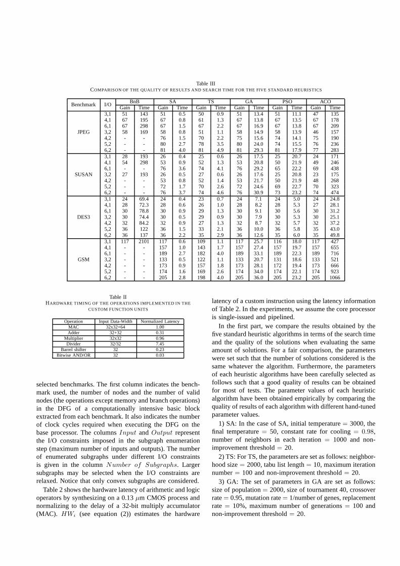
Table IIICOMPARISON OF THE QUALITY OF RESULTS AND SEARCH TIME FOR THE FIVE STANDARD HEURISTICS
Benchmark I/O BnB SA TS GA PSO ACOGain Time Gain Time Gain Time Gain Time Gain Time Gain Time
JPEG
3,1 51 143 51 0.5 50 0.9 51 13.4 51 11.1 47 1354,1 67 195 67 0.8 61 1.3 67 13.8 67 13.5 67 1786,1 67 298 67 1.5 67 2.2 67 16.9 67 13.8 67 2093,2 58 169 58 0.8 51 1.1 58 14.9 58 13.9 46 1574,2 - - 76 1.5 70 2.2 75 15.6 74 14.1 75 1905,2 - - 80 2.7 78 3.5 80 24.0 74 15.5 76 2366,2 - - 81 4.0 81 4.9 81 29.3 81 17.9 77 283
SUSAN
3,1 28 193 26 0.4 25 0.6 26 17.5 25 20.7 24 1714,1 54 298 53 0.9 52 1.3 53 20.8 50 21.9 49 2466,1 - - 76 3.6 74 4.1 76 29.2 65 22.2 69 4383,2 27 193 26 0.5 27 0.6 26 17.6 25 20.8 23 1754,2 - - 53 0.8 52 1.4 53 21.7 50 21.9 48 2685,2 - - 72 1.7 70 2.6 72 24.6 69 22.7 70 3236,2 - - 76 3.7 74 4.6 76 30.9 73 23.2 74 474
DES3
3,1 24 69.4 24 0.4 23 0.7 24 7.1 24 5.0 24 24.84,1 28 72.3 28 0.6 26 1.0 28 8.2 28 5.3 27 28.16,1 30 78.8 30 0.9 29 1.3 30 9.1 30 5.6 30 31.23,2 30 74.4 30 0.5 29 0.9 30 7.9 30 5.3 30 25.14,2 32 84.2 32 0.9 27 1.3 32 8.7 32 5.7 32 37.25,2 36 122 36 1.5 33 2.1 36 10.0 36 5.8 35 43.06,2 36 137 36 2.2 35 2.9 36 12.6 35 6.0 35 49.8
GSM
3,1 117 2101 117 0.6 109 1.1 117 25.7 116 18.0 117 4274,1 - - 157 1.0 143 1.7 157 27.4 157 19.7 157 6556,1 - - 189 2.7 182 4.0 189 33.1 189 22.3 189 7163,2 - - 133 0.5 122 1.1 133 20.7 131 18.6 133 5214,2 - - 173 0.9 157 1.8 173 28.1 172 19.4 173 6665,2 - - 174 1.6 169 2.6 174 34.0 174 22.1 174 9236,2 - - 205 2.8 198 4.0 205 36.0 205 23.2 205 1066
Table IIHARDWARE TIMING OF THE OPERATIONS IMPLEMENTED IN THE
CUSTOM FUNCTION UNITS
Operation Input Data-Width Normalized LatencyMAC 32x32+64 1.00Adder 32+32 0.31
Multiplier 32x32 0.96Divider 32/32 7.45
Barrel shifter 32 0.23Bitwise AND/OR 32 0.03
selected benchmarks. The first column indicates the bench-mark used, the number of nodes and the number of validnodes (the operations except memory and branch operations)in the DFG of a computationally intensive basic blockextracted from each benchmark. It also indicates the numberof clock cycles required when executing the DFG on thebase processor. The columnsInput andOutput representthe I/O constraints imposed in the subgraph enumerationstep (maximum number of inputs and outputs). The numberof enumerated subgraphs under different I/O constraintsis given in the columnNumber of Subgraphs. Largersubgraphs may be selected when the I/O constraints arerelaxed. Notice that only convex subgraphs are considered.
Table 2 shows the hardware latency of arithmetic and logicoperators by synthesizing on a 0.13µm CMOS process andnormalizing to the delay of a 32-bit multiply accumulator(MAC). HWi (see equation (2)) estimates the hardware
latency of a custom instruction using the latency informationof Table 2. In the experiments, we assume the core processoris single-issued and pipelined.
In the first part, we compare the results obtained by thefive standard heuristic algorithms in terms of the search timeand the quality of the solutions when evaluating the sameamount of solutions. For a fair comparison, the parameterswere set such that the number of solutions considered is thesame whatever the algorithm. Furthermore, the parametersof each heuristic algorithms have been carefully selected asfollows such that a good quality of results can be obtainedfor most of tests. The parameter values of each heuristicalgorithm have been obtained empirically by comparing thequality of results of each algorithm with different hand-tunedparameter values.
1) SA: In the case of SA, initial temperature= 3000, thefinal temperature= 50, constant rate for cooling= 0.98,number of neighbors in each iteration= 1000 and non-improvement threshold= 20.
2) TS: For TS, the parameters are set as follows: neighbor-hood size= 2000, tabu list length= 10, maximum iterationnumber= 100 and non-improvement threshold= 20.
3) GA: The set of parameters in GA are set as follows:size of population= 2000, size of tournament 40, crossoverrate= 0.95, mutation rate= 1/number of genes, replacementrate= 10%, maximum number of generations= 100 andnon-improvement threshold= 20.
0
20
40
60
80
100
(3,1) (4,1) (6,1) (3,2) (4,2) (5,2) (6,2)
Pe
rfo
rma
nce
ga
in
I/O Constraints
JPEG
SA
PSO
MPSO
ACO
MACO 0
20
40
60
80
100
(3,1) (4,1) (6,1) (3,2) (4,2) (5,2) (6,2)
Pe
rfo
rma
nce
ga
in
I/O Constraints
SUSAN
SA
PSO
MPSO
ACO
MACO
0
10
20
30
40
(3,1) (4,1) (6,1) (3,2) (4,2) (5,2) (6,2)
Pe
rfo
rma
nce
ga
in
I/O Constraints
DES3
SA
PSO
MPSO
ACO
MACO0
50
100
150
200
250
(3,1) (4,1) (6,1) (3,2) (4,2) (5,2) (6,2)
Pe
rfo
rma
nce
ga
in
I/O Constraints
GSM
SA
PSO
MPSO
ACO
MACO
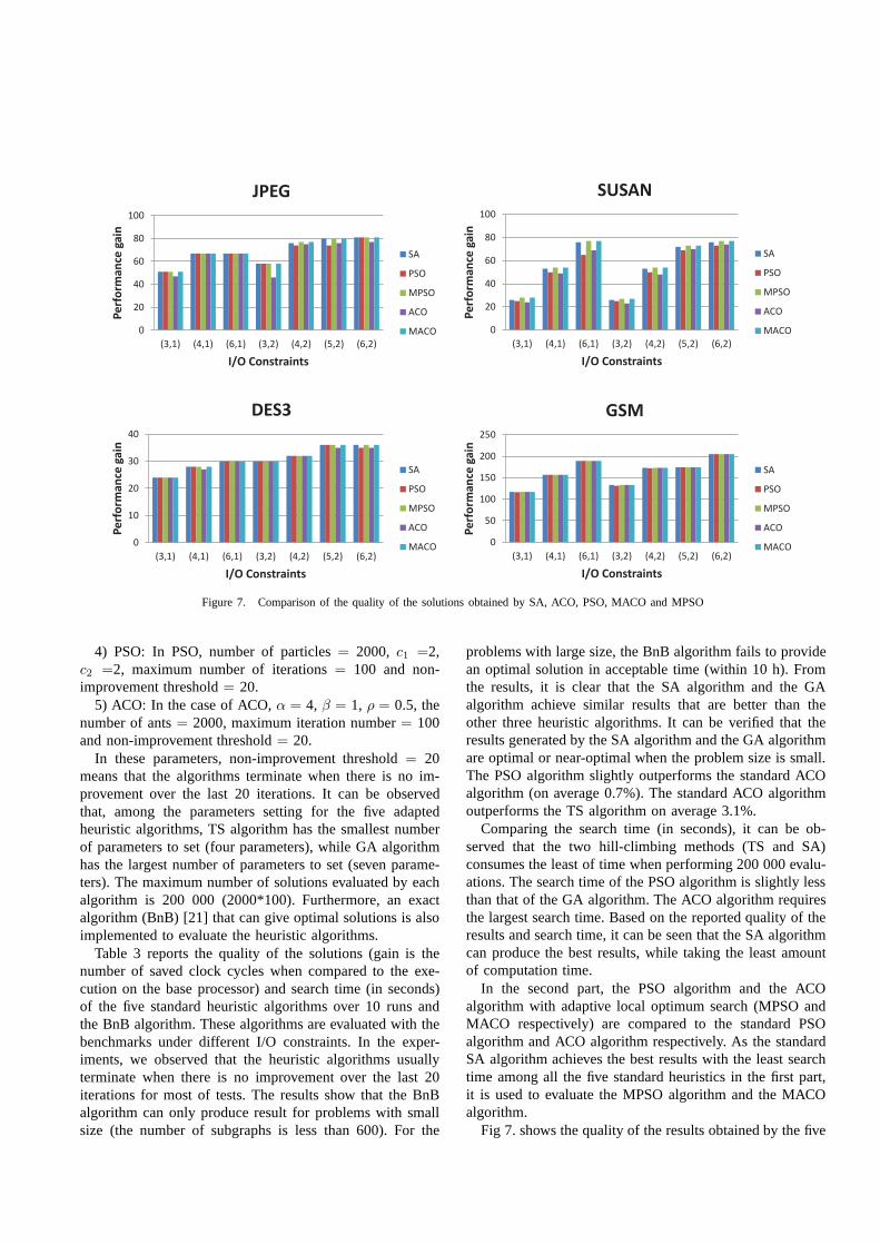
Figure 7. Comparison of the quality of the solutions obtained by SA, ACO, PSO, MACO and MPSO
4) PSO: In PSO, number of particles= 2000, c1 =2,c2 =2, maximum number of iterations= 100 and non-improvement threshold= 20.
5) ACO: In the case of ACO,α = 4, β = 1, ρ = 0.5, thenumber of ants= 2000, maximum iteration number= 100and non-improvement threshold= 20.
In these parameters, non-improvement threshold= 20means that the algorithms terminate when there is no im-provement over the last 20 iterations. It can be observedthat, among the parameters setting for the five adaptedheuristic algorithms, TS algorithm has the smallest numberof parameters to set (four parameters), while GA algorithmhas the largest number of parameters to set (seven parame-ters). The maximum number of solutions evaluated by eachalgorithm is 200 000 (2000*100). Furthermore, an exactalgorithm (BnB) [21] that can give optimal solutions is alsoimplemented to evaluate the heuristic algorithms.
Table 3 reports the quality of the solutions (gain is thenumber of saved clock cycles when compared to the exe-cution on the base processor) and search time (in seconds)of the five standard heuristic algorithms over 10 runs andthe BnB algorithm. These algorithms are evaluated with thebenchmarks under different I/O constraints. In the exper-iments, we observed that the heuristic algorithms usuallyterminate when there is no improvement over the last 20iterations for most of tests. The results show that the BnBalgorithm can only produce result for problems with smallsize (the number of subgraphs is less than 600). For the
problems with large size, the BnB algorithm fails to providean optimal solution in acceptable time (within 10 h). Fromthe results, it is clear that the SA algorithm and the GAalgorithm achieve similar results that are better than theother three heuristic algorithms. It can be verified that theresults generated by the SA algorithm and the GA algorithmare optimal or near-optimal when the problem size is small.The PSO algorithm slightly outperforms the standard ACOalgorithm (on average 0.7%). The standard ACO algorithmoutperforms the TS algorithm on average 3.1%.
Comparing the search time (in seconds), it can be ob-served that the two hill-climbing methods (TS and SA)consumes the least of time when performing 200 000 evalu-ations. The search time of the PSO algorithm is slightly lessthan that of the GA algorithm. The ACO algorithm requiresthe largest search time. Based on the reported quality of theresults and search time, it can be seen that the SA algorithmcan produce the best results, while taking the least amountof computation time.
In the second part, the PSO algorithm and the ACOalgorithm with adaptive local optimum search (MPSO andMACO respectively) are compared to the standard PSOalgorithm and ACO algorithm respectively. As the standardSA algorithm achieves the best results with the least searchtime among all the five standard heuristics in the first part,it is used to evaluate the MPSO algorithm and the MACOalgorithm.
Fig 7. shows the quality of the results obtained by the five

0.5
2
8
32
128
512
(3,1) (4,1) (6,1) (3,2) (4,2) (5,2) (6,2)
Se
arc
h t
ime
(se
con
ds)
I/O Constraints
JPEG
PSO
MPSO
ACO
MACO
SA0.25
1
4
16
64
256
(3,1) (4,1) (6,1) (3,2) (4,2) (5,2) (6,2)
Se
arc
h t
ime
(se
con
ds)
I/O Constraints
SUSAN
PSO
MPSO
ACO
MACO
SA
0.25
0.5
1
2
4
8
16
32
64
(3,1) (4,1) (6,1) (3,2) (4,2) (5,2) (6,2)Se
arc
h t
ime
(se
con
ds)
I/O Constraints
DES3
PSO
MPSO
ACO
MACO
SA0.5
2
8
32
128
512
2048
(3,1) (4,1) (6,1) (3,2) (4,2) (5,2) (6,2)Se
arc
h t
ime
(se
con
ds)
I/O Constraints
GSM
PSO
MPSO
ACO
MACO
SA
Figure 8. Comparison of the search time consumed by SA, ACO, PSO, MACO and MPSO
algorithms in 10 runs1. Based on the results, we can see thatthe MPSO algorithm and the MACO algorithm outperformthe standard PSO algorithm and the standard ACO algorithmon average 2.1% and 2.9% respectively. Furthermore, theMPSO algorithm and MACO algorithm achieve the sameresults that are slightly better than the results obtained bythe SA algorithm. In particular, the SA algorithm can notreach the optimal results for the benchmark SUSAN whenthe I/O is (3,1),(4,1) or (3,2), while the MPSO algorithmand MACO algorithm can produce the optimal results (thesame results as BnB).
Fig 8. compares SA, PSO, MPSO, ACO and MACOalgorithms in terms of average search time. The maximumnumber of solutions evaluated by each algorithm is 200 000.The results are obtained from 10 runs. From the results, wecan see that the SA algorithm is the fastest among the fivealgorithms. It can be also observed that the computationtime of the MPSO algorithm and the MACO algorithm aremuch more less than that of the standard PSO algorithmand the standard ACO algorithm. The MACO algorithm (orMPSO) with adaptive local optimum search builds 20 000solutions using the standard ACO (or PSO) optimization andthe other 180 000 solutions using proposed local optimum
1the standard PSO algorithm, the standard ACO algorithm, theMPSOalgorithm, the MACO algorithm and the standard SA algorithm.
search. As the optimum search method produce a neighborsolution much faster than the standard ACO or PSO op-timization, the overall search time is significantly reducedby the MACO algorithm. On average, the MACO algorithmis 8.7 times faster than the standard ACO algorithm. TheMPSO algorithm is 3.9 times faster than the standard PSOalgorithm. Combining the quality of the results shown in Fig6. and the search time presented in Fig 7., we can concludethat the the MPSO algorithm and the MACO algorithmwith adaptive local optimum search can find better resultsin shorter time than the standard PSO algorithm and thestandard ACO algorithm.
VI. EXTRA COMMENTS
When the given hardware area is limited, it is necessaryto take into account the area constraint. Although the areaconstraint is not considered in these experiments, the heuris-tic algorithms presented in this paper are able to take it intoaccount with few modifications. In the case of consideringarea constraint, a set of patterns should be generated. The setof patterns is generally collected using a graph isomorphismalgorithm. Given two subgraphsa andb, if a is isomorphicto b, a patternTi is created, and the subgraphsa and bare recorded in the patternTi as instances. If two or moreinstances of a pattern are selected, they may share the same
hardware implementation of their corresponding pattern (thisis the case of reusing hardware). We can use the followinginequality to express the area constraint:
k∑
i=1
ciyi ≤ A (15)
where yi = 1 indicates that one or more instances ofthe patternTi are selected, whileyi = 0 indicates that noinstance ofTi is selected.ci is the area cost of the hardwareimplementation of a patternTi. A is a given maximum areaconstraint. In the heuristic algorithms, the area cost of asolution should be calculated and the area constraint can beused to guide the construction of solutions. It is noteworthythat the upper bound on the number of feasible solutionsshould be less than3n/3 when taking into account the areaconstraint.
For each of the experimented heuristic algorithms, modi-fied versions that may improve quality of results or requireless runtime can be found in the literature. However, in thispaper the main objective is to compare the standard meta-heuristic algorithms when applied to the custom instructionselection problem. Implementing modified versions of theseheuristic algorithms is out of the scope of this paper. Peoplewho are interested can find details for example in [21]–[23],[38].
In this paper, we have proved the upper bound on thenumber of feasible solutions with respect to non-overlappingconstraint and acyclicity constraint, however, allowing over-lapping between selected subgraphs may bring more per-formance improvement. In this scenario, it is interesting toknow the upper bound on the number of feasible solutionswhen overlapping is allowed. It is also necessary to comparethe difference on the performance improvement and thesearch time between allowing overlapping and disallowingoverlapping during subgraph selection. These can be part ofour future work.
VII. C ONCLUSIONS
In this paper, the upper bound on the number of fea-sible solutions for the subgraph selection problem hasbeen given and formally proved. We have introduced fivepopular heuristic algorithms, namely simulated annealing,tabu search, genetic algorithm, particle swarm optimizationalgorithm and ant colony optimization algorithm, for solvingthe subgraph selection problem. Extensive experiments withreal-life benchmarks have been carried out to evaluate theadvantages and disadvantages of the five heuristic algorithmsin terms of runtime performance and quality of the results.Furthermore, we have also implemented an adaptive localoptimum search strategy for particle swarm optimizationalgorithm and ant colony optimization algorithm, which canfurther improve the quality of the solutions. Future workwill deal with the inclusion of area constraint and allowingoverlapping in the heuristic algorithms.
VIII. A CKNOWLEDGEMENT
We are grateful to the anonymous referees for valuablesuggestions and comments which helped us to improve thepaper. The authors would like to thank the various grantsfrom the National Natural Science Foundation of China (No.61404069 and No. 61172144) and the Scientific ResearchFoundation for Ph.D. of Liaoning Province (No. 20141140).
REFERENCES
[1] C. Galuzzi, K. Bertels. The Instruction-Set Extension Problem:A Survey. ARC 2008, pp. 209-220.
[2] K. Atasu, L. Pozzi, and P. Ienne. Automatic application-specific instruction-set extensions under microarchitecturalconstraints. DAC 2003, pp. 256-261.
[3] L. Pozzi, K. Atasu, and P. Ienne. Exact and approximatealgorithms for the extension of embedded processor instructionsets. IEEE Trans. Comput.Aided Design Integr. Circuits Syst.25(7), 2006, pp. 1209-1229.
[4] C. Xiao, E. Casseau. An efficient algorithm for custom instruc-tion enumeration. GLSVLSI 2011, pp. 187-192.
[5] C. Xiao, E. Casseau. Exact custom instruction enumerationfor extensible processors. Integration, the VLSI Journal 45 (3),2012, pp. 263-270.
[6] X. Chen, D.L. Maskell, Y. Sun. Fast identification of custominstructions for extensible processors. IEEE Transactions onComputer-Aided Design of Integrated Circuits and Systems,26(2), 2007, pp. 359-368.
[7] P. Bonzini, L. Pozzi. Polynomial-time subgraph enumerationfor automated instruction set extension. DATE 2007, pp. 1331-1336.
[8] T. Li, Z. Sun, W. Jigang. Fast enumeration of maximal validsubgraphs for custom-instruction identification. CASES 2009,pp. 29-36.
[9] A.K. Verma, P. Brisk, P. Ienne. Fast, nearly optimal ISEidentification with I/O serialization through maximal cliqueenumeration. IEEE Transactions on Computer-Aided Designof Integrated Circuits and Systems, 29(3), 2010, pp. 341-354.
[10] J. Reddington, K. Atasu. Complexity of computing convexsubgraphs in custom instruction synthesis. IEEE Transactionson Very Large Scale Integration (VLSI) Systems. 20(12), 2012,pp. 2337-2341.
[11] N. Clark, A. Hormati, S. Mahlke, and S. Yehia. Scalable sub-graph mapping for acyclic computation accelerators. CASES2006, pp. 147-157.
[12] J. Cong et al. Application-specific instruction generation forconfigurable processor architectures. FPGA 2004, pp. 183-189.
[13] T. Mitra, Y. Pan. Satisfying real-time constraints with custominstructions. CODES+ISSS 2005, pp. 166-171.
[14] C. Galuzzi, E.M. Panainte, Y. Yankova, K. Bertels, S. Vassil-iadis. Automatic selection of application-specific instruction-set extensions. CODES+ISSS 2006, pp.160-165.
[15] K. Atasu, G. Dundar, C. Ozturan. An integer linear pro-gramming approach for identifying instruction-set extensions.CODES+ISSS 2005, pp.172-177.
[16] K. Martin, C. Wolinski, K. Kuchcinski, A. Floch, F. Charot:Constraint Programming Approach to Reconfigurable Proces-sor Extension Generation and Application Compilation. TRET-S 5 (2), 2012.
[17] M. A. Arslan, K. Kuchcinski. Instruction Selection andScheduling for DSP Kernels on Custom Architectures. DSD2013, pp. 821-828.
[18] R. Kastner, A. Kaplan, S. Ogrenci Memik, and E. Bo-zorgzadeh. Instruction generation for hybrid reconfigurablesystems. ACM Trans. Des. Autom. Electron. Syst. 7(4), 2002,pp. 605-627.
[19] C. Wolinski, K. Kuchcinski. Automatic Selection ofApplication-Specific Reconfigurable Processor Extensions.DATE 2008, pp. 1214-1219.
[20] N. Clark, M. Kudlur, P. Hyunchul, S. Mahlke, K. Flautner.Application-Specific Processing on a General-Purpose CoreviaTransparent Instruction Set Customization. MICRO 2004, pp.30-40.
[21] T. Li, J. Wu, S. Lam, T. Srikanthan, and X. Lu. Selectingprofitable custom instructions for reconfigurable processors. J.Syst. Archit. 56(8), 2010, pp. 340-351.
[22] M. Kamal, K.N. Amiri, A. Kamran A. Dual-purpose custominstruction identification algorithm based on particle swarmoptimization. ASAP 2010, pp. 159-166.
[23] F. Ferrandi, P.L. Lanzi, C. Pilato C. Ant colony heuristic formapping and scheduling tasks and communications on hetero-geneous embedded systems. IEEE Transactions on Computer-Aided Design of Integrated Circuits and Systems. 29(6), 2010,pp.911-924.
[24] I.W. Wu, Z.Y. Chen, J.J. Shann J J. Instruction set extensionexploration in multiple-issue architecture. DATE 2008, pp.764-769.
[25] H. Lin. Multi-objective Application-specific Instruction setProcessor Design: Towards High Performance, Energy-efficient, and Secure Embedded Systems (2011). DoctoralDissertations.
[26] K. Atasu, W. Luk, O. Mencer, C. Ozturan, G.Dundar. FISH:Fast instruction synthesis for custom processors. IEEE Trans-actions on Very Large Scale Integration (VLSI) Systems, 20(1),2012, pp. 52-65.
[27] Y. Guo, G.J.M. Smit, H. Broersma. A graph covering algo-rithm for a coarse grain reconfigurable system. LCTES 2003,pp. 199-208.
[28] J.W. Moon, L. Moser. On cliques in graphs. Israel journal ofMathematics, 1965, 3(1): pp. 23-28.
[29] S., Kirkpatrick, C.D. Gelatt, M. P. Vecchi. Optimization bysimmulated annealing. Science. 220(4598), 1983, pp. 671-680.APA
[30] F. Glover. Tabu search: A tutorial. Interfaces, 1990, 20(4): pp.74-94.
[31] T. Wiangtong, P. Cheung, and W. Luk. Comparing threeheuristic search methods for functional partitioning inhardware-software codesign. Des. Autom. Embed. Syst. 6(4),2002, pp.425-449.
[32] John H. Holland. Adaptation in natural and artificial systems.Univ. of Mochigan Press, 1975.
[33] J. Kennedy, R. Eberhart. Particle swarm optimization.IEEEInternational Conference on Neural Networks 1995, pp.1942-1948.
[34] M. Dorigo, V. Maniezzo, and A. Colorni. Ant system: opti-mization by a colony of cooperating agents. Trans. Sys. Man.Cyber. Part B 26, 1996, pp. 29-41.
[35] GeCoS: Generic compiler suite - http://gecos.gforge.inria.fr/[36] M. R. Guthaus, J. S. Ringenberg, D. Ernst, T. M.Austin,
T. Mudge, and R. B. Brown. Mibench: A free,commerciallyrepresentative embedded benchmark suite. WWC 2001, pp. 3-14.
[37] C. Lee, M. Potkonjak, and W. H. Mangione-smith. Media-bench: A tool for evaluating and synthesizing multimedia andcommunications systems. MICRO 1997, pp 330-335.
[38] D. Pham, D. Karaboga. Intelligent optimisation techniques:genetic algorithms, tabu search, simulated annealing and neuralnetworks. Springer Science& Business Media, 2012.