heuristic algorithms for graph coloring problems
TRANSCRIPT

HAL Id: tel-02136810https://tel.archives-ouvertes.fr/tel-02136810
Submitted on 22 May 2019
HAL is a multi-disciplinary open accessarchive for the deposit and dissemination of sci-entific research documents, whether they are pub-lished or not. The documents may come fromteaching and research institutions in France orabroad, or from public or private research centers.
L’archive ouverte pluridisciplinaire HAL, estdestinée au dépôt et à la diffusion de documentsscientifiques de niveau recherche, publiés ou non,émanant des établissements d’enseignement et derecherche français ou étrangers, des laboratoirespublics ou privés.
Heuristic Algorithms for Graph Coloring ProblemsWen Sun
To cite this version:Wen Sun. Heuristic Algorithms for Graph Coloring Problems. Data Structures and Algorithms[cs.DS]. Université d’Angers, 2018. English. NNT : 2018ANGE0027. tel-02136810

THESE DE DOCTORAT DE L'UNIVERSITE D'ANGERS COMUE UNIVERSITE BRETAGNE LOIRE ECOLE DOCTORALE N° 601 Mathématiques et Sciences et Technologies de l'Information et de la Communication Spécialité : Informatique, section CNU 27 Par
Wen SUN
Heuristic Algorithms for Graph Coloring Problems Thèse présentée et soutenue à Angers, le 29/11/2018 Unité de recherche : Laboratoire d'Étude et de Recherche en Informatique d'Angers (LERIA)
Rapporteurs avant soutenance : Djamal HABET MC HDR, Université d'Aix-Marseille Olivier BAILLEUX MC HDR, Université de Bourgogne Composition du Jury : Examinateurs : Béatrice DUVAL Professeur, Université d'Angers Djamal HABET MC HDR, Université d'Aix-Marseille
Marc SCHOENAUER Directeur de Recherche, INRIA Olivier BAILLEUX MC HDR, Université de Bourgogne Dir. de thèse : Jin-Kao HAO Professeur, Université d'Angers Co-dir. de thèse : Alexandre CAMINADA Professeur, Université Côte d’Azur


Contents
General Introduction 7
1 Introduction 111.1 Graph coloring problem . . . . . . . . . . . . . . . . . . . . . . . . . . . . . . . . . . 12
1.1.1 Problem Introduction . . . . . . . . . . . . . . . . . . . . . . . . . . . . . . . 121.1.2 Exact algorithm . . . . . . . . . . . . . . . . . . . . . . . . . . . . . . . . . . . 121.1.3 Heuristic algorithm . . . . . . . . . . . . . . . . . . . . . . . . . . . . . . . . . 131.1.4 Summary . . . . . . . . . . . . . . . . . . . . . . . . . . . . . . . . . . . . . . 14
1.2 Equitable coloring problem . . . . . . . . . . . . . . . . . . . . . . . . . . . . . . . . 151.2.1 Theoretical Studies . . . . . . . . . . . . . . . . . . . . . . . . . . . . . . . . . 151.2.2 Exact approaches . . . . . . . . . . . . . . . . . . . . . . . . . . . . . . . . . . 151.2.3 Heuristic approaches . . . . . . . . . . . . . . . . . . . . . . . . . . . . . . . . 161.2.4 Summary . . . . . . . . . . . . . . . . . . . . . . . . . . . . . . . . . . . . . . 16
1.3 Weighted vertex coloring problem . . . . . . . . . . . . . . . . . . . . . . . . . . . . 171.3.1 Exact approaches . . . . . . . . . . . . . . . . . . . . . . . . . . . . . . . . . . 181.3.2 Heuristic approaches . . . . . . . . . . . . . . . . . . . . . . . . . . . . . . . . 181.3.3 Summary . . . . . . . . . . . . . . . . . . . . . . . . . . . . . . . . . . . . . . 18
1.4 k-vertex critical subgraphs problem . . . . . . . . . . . . . . . . . . . . . . . . . . . . 191.4.1 Problem Introduction . . . . . . . . . . . . . . . . . . . . . . . . . . . . . . . 191.4.2 Exact approaches . . . . . . . . . . . . . . . . . . . . . . . . . . . . . . . . . . 201.4.3 Heuristic approaches . . . . . . . . . . . . . . . . . . . . . . . . . . . . . . . . 201.4.4 Summary . . . . . . . . . . . . . . . . . . . . . . . . . . . . . . . . . . . . . . 20
2 A reduction-based memetic algorithm for GCP 212.1 Introduction . . . . . . . . . . . . . . . . . . . . . . . . . . . . . . . . . . . . . . . . . 232.2 Memetic algorithm for the GCP . . . . . . . . . . . . . . . . . . . . . . . . . . . . . . 23
2.2.1 General approach . . . . . . . . . . . . . . . . . . . . . . . . . . . . . . . . . . 232.2.2 Population initialization . . . . . . . . . . . . . . . . . . . . . . . . . . . . . . 242.2.3 The adaptive multi-parent crossover procedure . . . . . . . . . . . . . . . . 272.2.4 Backbone-based group matching . . . . . . . . . . . . . . . . . . . . . . . . . 272.2.5 Weight tabu search improvement . . . . . . . . . . . . . . . . . . . . . . . . . 302.2.6 Uncoarsening phase . . . . . . . . . . . . . . . . . . . . . . . . . . . . . . . . 312.2.7 Pool updating strategy . . . . . . . . . . . . . . . . . . . . . . . . . . . . . . . 32
2.3 Experimental results and comparisons . . . . . . . . . . . . . . . . . . . . . . . . . . 322.3.1 Benchmark instances . . . . . . . . . . . . . . . . . . . . . . . . . . . . . . . . 332.3.2 Experiment settings . . . . . . . . . . . . . . . . . . . . . . . . . . . . . . . . 332.3.3 Comparison with state-of-the-art algorithms . . . . . . . . . . . . . . . . . . 352.3.4 Comparative results on easy instances . . . . . . . . . . . . . . . . . . . . . . 352.3.5 Comparative results on difficult instances . . . . . . . . . . . . . . . . . . . . 36
2.4 Analysis . . . . . . . . . . . . . . . . . . . . . . . . . . . . . . . . . . . . . . . . . . . 37
3

4 CONTENTS
2.4.1 Effectiveness of the number of parents for RMA . . . . . . . . . . . . . . . . 372.4.2 Effectiveness of the different matching strategies for RMA . . . . . . . . . . 372.4.3 Effectiveness of the perturbation operation . . . . . . . . . . . . . . . . . . . 38
2.5 Conclusions . . . . . . . . . . . . . . . . . . . . . . . . . . . . . . . . . . . . . . . . . 38
3 On feasible and infeasible search for ECP 413.1 Introduction . . . . . . . . . . . . . . . . . . . . . . . . . . . . . . . . . . . . . . . . . 423.2 Basic definitions . . . . . . . . . . . . . . . . . . . . . . . . . . . . . . . . . . . . . . . 423.3 Feasible and infeasible search algorithm for ECP . . . . . . . . . . . . . . . . . . . . 43
3.3.1 General approach . . . . . . . . . . . . . . . . . . . . . . . . . . . . . . . . . . 433.3.2 Searching equity-feasible solutions . . . . . . . . . . . . . . . . . . . . . . . . 443.3.3 Searching equity-infeasible solutions . . . . . . . . . . . . . . . . . . . . . . . 453.3.4 Perturbation of infeasible search . . . . . . . . . . . . . . . . . . . . . . . . . 47
3.4 Experimental results and comparisons . . . . . . . . . . . . . . . . . . . . . . . . . . 483.4.1 Experiment settings . . . . . . . . . . . . . . . . . . . . . . . . . . . . . . . . 483.4.2 Comparison with state-of-the-art algorithms . . . . . . . . . . . . . . . . . . 48
3.5 Analysis . . . . . . . . . . . . . . . . . . . . . . . . . . . . . . . . . . . . . . . . . . . 493.5.1 Analysis of the penalty coefficient ϕ . . . . . . . . . . . . . . . . . . . . . . . 493.5.2 Impact of the perturbation operation . . . . . . . . . . . . . . . . . . . . . . . 49
3.6 Conclusions . . . . . . . . . . . . . . . . . . . . . . . . . . . . . . . . . . . . . . . . . 52
4 Adaptive feasible and infeasible search for WVCP 534.1 Introduction . . . . . . . . . . . . . . . . . . . . . . . . . . . . . . . . . . . . . . . . . 544.2 Adaptive feasible and infeasible search for the WVCP . . . . . . . . . . . . . . . . . 54
4.2.1 General approach . . . . . . . . . . . . . . . . . . . . . . . . . . . . . . . . . . 544.2.2 Initial solution . . . . . . . . . . . . . . . . . . . . . . . . . . . . . . . . . . . . 554.2.3 Search space and penalty-based evaluation function . . . . . . . . . . . . . . 554.2.4 Searching feasible and infeasible solutions with tabu search . . . . . . . . . 574.2.5 Perturbation strategy . . . . . . . . . . . . . . . . . . . . . . . . . . . . . . . . 594.2.6 Connections with existing studies . . . . . . . . . . . . . . . . . . . . . . . . 60
4.3 Experimental results and comparisons . . . . . . . . . . . . . . . . . . . . . . . . . . 604.3.1 Benchmark instances . . . . . . . . . . . . . . . . . . . . . . . . . . . . . . . . 604.3.2 Experimental settings . . . . . . . . . . . . . . . . . . . . . . . . . . . . . . . 614.3.3 Computational results and comparisons with state-of-the-art algorithms . . 62
4.4 Analysis . . . . . . . . . . . . . . . . . . . . . . . . . . . . . . . . . . . . . . . . . . . 654.4.1 Impact of the penalty coefficient . . . . . . . . . . . . . . . . . . . . . . . . . 664.4.2 Benefit of searching both feasible and infeasible solutions . . . . . . . . . . 674.4.3 Impact of the perturbation operation . . . . . . . . . . . . . . . . . . . . . . . 68
4.5 Conclusions . . . . . . . . . . . . . . . . . . . . . . . . . . . . . . . . . . . . . . . . . 69
5 Iterated backtrack removal search for finding k-VCS 715.1 Introduction . . . . . . . . . . . . . . . . . . . . . . . . . . . . . . . . . . . . . . . . . 725.2 Notations . . . . . . . . . . . . . . . . . . . . . . . . . . . . . . . . . . . . . . . . . . . 725.3 The Iterated Backtrack-based Removal Algorithm . . . . . . . . . . . . . . . . . . . 73
5.3.1 General structure of the IBR algorithm . . . . . . . . . . . . . . . . . . . . . . 735.3.2 The removal algorithm . . . . . . . . . . . . . . . . . . . . . . . . . . . . . . . 765.3.3 Heuristic coloring algorithm . . . . . . . . . . . . . . . . . . . . . . . . . . . 765.3.4 Backtrack-based removal approach . . . . . . . . . . . . . . . . . . . . . . . 775.3.5 Perturbation operator of backtrack-based removal algorithm . . . . . . . . . 785.3.6 Update procedure . . . . . . . . . . . . . . . . . . . . . . . . . . . . . . . . . 79
5.4 Experimental results and analysis . . . . . . . . . . . . . . . . . . . . . . . . . . . . . 81

CONTENTS 5
5.4.1 Experiment settings . . . . . . . . . . . . . . . . . . . . . . . . . . . . . . . . 815.4.2 Instances and experimental settings . . . . . . . . . . . . . . . . . . . . . . . 835.4.3 Comparison with state of the art algorithm . . . . . . . . . . . . . . . . . . . 83
5.5 Analysis and discussions . . . . . . . . . . . . . . . . . . . . . . . . . . . . . . . . . . 855.5.1 Effectiveness of different backtrack strategies for k-VCS detection . . . . . . 865.5.2 Effectiveness of perturbation for k-VCS detection . . . . . . . . . . . . . . . 865.5.3 Effectiveness of backtrack for k-VCS detection . . . . . . . . . . . . . . . . . 87
5.6 Conclusion . . . . . . . . . . . . . . . . . . . . . . . . . . . . . . . . . . . . . . . . . . 87
General Conclusion 89
Appendix 93
List of Publications 95
List of Figures 97
List of Tables 100
References 109


General Introduction
Context
Graph vertex coloring problems are known to be very general and useful models to formulatenumerous practical problems [Lewis, 2015]. Given an undirected graph G = (V, E) with thevertex set V = 1, 2, . . . , n, the edge set E ∈ V × V, graph vertex coloring problems typicallyinvolve assigning a color to each vertex of V such that two vertices linked by an edge must receivedifferent colors while optimizing a given optimization objective.
This thesis focuses on four generalized graph coloring problems, namely the graph color-ing problem (GCP), the equitable coloring problem (ECP), the weighted vertex coloring problem(WVCP) and the k-vertex critical subgraphs (k-VCS). The first one is the most basic graph coloringproblem. The ECP requires that the sizes of two arbitrary color classes differ in at most one unitwhile the WVCP aims to minimize the sum of the largest weights of the vertices of each colorclass. The k-VCS is to find a subgraph H of G with minimum vertices such that removing anyvertex from the subgraph H decreases its chromatic number.
These four problems are practically relevant since they have wide applications in real worldsuch as garbage collection, load balancing, timetabling, scheduling, operating system, manufac-turing, etc.
From the perspective of computational theory, graph coloring problems belong to the class ofthe NP-hard problems, meaning that optimal solutions cannot be found in polynomial time in thegeneral case. For solving large and challenging problem instances, heuristic and metaheuristicapproaches are commonly used with the purpose of finding sub-optimal solutions in reasonabletime. In this thesis, we investigate hybrid metaheuristic approaches to effectively solve the fourproblems of interest aforementioned. Each proposed algorithm will be thoroughly documentedwith extensive computational experiments.
Objectives
One of the main objectives of this thesis is to develop high-performance hybrid metaheuristicalgorithms that improve the state-of-the-art solutions for each problem considered. The mainobjective can be further divided into several specific objectives:
— Develop an effective reduction approach based on a backbone coarsening operator.— Devise feasible and infeasible search algorithms that allow search process to cross the fea-
sibility boundaries to explore the enlarged search space.— Develop an adaptive mechanism to further control feasible and infeasible searches.— Extend the removal strategy with backtracking mechanism to reconsider some removed
vertices and investigate a perturbation strategy to escape local optima traps.— Evaluate the proposed algorithms on a wide range of benchmark instance and perform a
comprehensive comparison with the state-of-the-art algorithm.
7

Contributions
The main contributions of this thesis are summarized below:— For the graph coloring problem, we proposed a reduction-based memetic algorithm (RMA)
which integrates several original ingredients. First, we devise a backbone-based crossoveroperator to merge certain vertices. This operator aims to reduce the current graph andpreserve common contributive objects that are shared by parent solutions. Second, to ex-plore efficiently the search space around an offspring solution generated by the crossoveroperator, we propose a weighted tabu search algorithm, Finally, we apply a perturbationstrategy to escape from the region of the local optimum. Experiment results on 39 popularDIMACS and COLOR02-04 benchmark instances, which are commonly used to test graphcoloring algorithms in the literature, showed that RMA is competitive in terms of solutionquality and run-time efficiency compared with state-of-the-art algorithms in the literature.
— For the equitable coloring problem, we propose a feasible and infeasible search algorithm(FISA). FISA combines an equity-feasible search phase where only equitable colorings areconsidered and an equity-infeasible search phase where the search is enlarged to includenon-equitable solutions. To guide the equity-infeasible search phase (which is based ontabu search), we devise an extended fitness function that uses a penalty to discourage can-didate solutions which violate the equity constraint. A perturbation procedure is adoptedas a diversification method to help the algorithm explore new search regions. We assessthe performance of the FISA algorithm on the set of 73 benchmark instances from DIMACSand COLOR competitions and present comparative results with respect to state-of-the-artalgorithms. Computational results showed that FISA performs very well by finding 9 newupper bounds and matching the best-known results for the remaining instances except onecase. This study demonstrates the benefit of examining both equity-feasible and equity-infeasible solutions for solving the ECP by using the mixed search strategy.
— For the weighted vertex coloring problem, we develop an adaptive feasible and infeasi-ble search algorithm (AFISA). Like FISA, the proposed algorithm relies on a mixed searchstrategy exploring both feasible and infeasible solutions. To prevent the search from goingtoo far away from the feasible boundary, we design an adaptive penalty-based evaluationfunction that is used to guide the search for an effective examination of candidate solu-tions, by enabling the search to oscillate between feasible and infeasible regions. To ex-plore a given search zone, we rely on the popular tabu search meta heuristic [Glover, 1989;Glover, 1990]. We assess the proposed algorithm on 111 benchmark instances from liter-atures (one set of 46 instances from the DIMACS and COLOR competitions and two setsof 65 instances from matrix-decomposition problems). We report especially 5 improvedbest solutions (new upper bounds). We also present new results on an additional set of 50larger instances.
— For the k-VCS problem, we propose an iterated backtrack-based removal (IBR) algorithm tosolve it. IBR adopts the popular removal strategy that reduces current graph by tentativelymoving vertices to the set of uncritical vertices. Although such an idea has been proved tobe very effective for finding a k-VCS for a given graph G, the status of some vertices aresometimes irreversibly misclassified, leading to meaningless result. A backtracking mech-anism is proposed to expand the current subgraph by adding back some vertices. We alsodevise a perturbation strategy to reconsider some vertices that would have been incorrectlyidentified as critical ones. Experiment results on 80 popular DIMACS and COLOR02-04benchmark instances, which are commonly used to test k-VCS algorithms in the literature,show that IBR is very competitive in terms of solution quality and run-time efficiency com-pared with state-of-the-art algorithms in the literature. Specifically, the proposed algorithmimproves the best-known solution for 9 graphs (improves the lower bound for 6 instances,
8

at the same k, IBR obtains a better solution (smaller size of k-VCS) for 8 instances), matchesthe best results for other 70 instances, and obtains a slightly worse result only in one case.
Organization
The manuscript is organized in the following way:— In the first chapter, we introduce the four graph coloring problems considered in this thesis,
i.e., graph coloring, equitable coloring, weighted vertex coloring and k-vertex-critical sub-graphs. For each problem, we also provide a brief overview of solution methods, includingapproximation algorithms, exact algorithms and heuristic/metaheuristic algorithms.
— In the second chapter, we present the RMA algorithm for the graph coloring problem.We first describe in detail the main components of the proposed approach that integratesa greedy initial procedure, a backbone-based coarsening operator, a weight-based tabusearch algorithm, an uncoarsening phase and the pool updating rule. Then, we presentexperimental results and comparisons with the state-of-the-art algorithms to show the ef-ficacy of the proposed algorithm and discuss the impacts of some key components.
— In the third chapter, we study the equitable coloring problem. This chapter begins with ashort introduction. After a detailed description of each component of the proposed FISAalgorithm, we show experimental studies on a set of 73 benchmark instances to assess theeffectiveness of the proposed FISA algorithm by comparing it with other best performingalgorithms. An analysis of the key ingredients is presented allowing us to understand thebehavior of all components in the proposed algorithm.
— In the fourth chapter, we consider the weighted vertex coloring problem and present theadaptive feasible and infeasible search algorithm (AFISA) to solve it. After introducingthe main scheme of the proposed algorithm, we explain each of its internal components.Computational comparisons with other algorithms and analysis of different componentsare presented.
— In the last chapter, we present an iterated backtrack-based removal (IBR) heuristic to find k-VCS for a given graph. We firstly describe in detail the main components of the proposedapproach including the removal strategy, a backtracking mechanism and a perturbationstrategy. Then, we provide an experimental study of the new algorithms, as well as com-parisons with state-of-the-art algorithms. Finally, we study some key ingredients of theproposed approach.
9


1Introduction
Graph coloring problems are a class of well-known NP-hard combinatorial optimization prob-lems with a wide range of applications. In this chapter, four graph coloring problems that arestudied in this thesis are introduced: classic graph coloring, equitable coloring, weighted vertexcoloring and k-vertex-critical subgraphs. A brief introduction for each problem is given first andthen state-of-the-art approaches for solving these problems in the literature are reviewed.
Contents1.1 Graph coloring problem . . . . . . . . . . . . . . . . . . . . . . . . . . . . . . . . . . 12
1.1.1 Problem Introduction . . . . . . . . . . . . . . . . . . . . . . . . . . . . . . . 121.1.2 Exact algorithm . . . . . . . . . . . . . . . . . . . . . . . . . . . . . . . . . . . 121.1.3 Heuristic algorithm . . . . . . . . . . . . . . . . . . . . . . . . . . . . . . . . . 131.1.4 Summary . . . . . . . . . . . . . . . . . . . . . . . . . . . . . . . . . . . . . . 14
1.2 Equitable coloring problem . . . . . . . . . . . . . . . . . . . . . . . . . . . . . . . . 151.2.1 Theoretical Studies . . . . . . . . . . . . . . . . . . . . . . . . . . . . . . . . . 151.2.2 Exact approaches . . . . . . . . . . . . . . . . . . . . . . . . . . . . . . . . . . 151.2.3 Heuristic approaches . . . . . . . . . . . . . . . . . . . . . . . . . . . . . . . . 161.2.4 Summary . . . . . . . . . . . . . . . . . . . . . . . . . . . . . . . . . . . . . . 16
1.3 Weighted vertex coloring problem . . . . . . . . . . . . . . . . . . . . . . . . . . . . 171.3.1 Exact approaches . . . . . . . . . . . . . . . . . . . . . . . . . . . . . . . . . . 181.3.2 Heuristic approaches . . . . . . . . . . . . . . . . . . . . . . . . . . . . . . . . 181.3.3 Summary . . . . . . . . . . . . . . . . . . . . . . . . . . . . . . . . . . . . . . 18
1.4 k-vertex critical subgraphs problem . . . . . . . . . . . . . . . . . . . . . . . . . . . 191.4.1 Problem Introduction . . . . . . . . . . . . . . . . . . . . . . . . . . . . . . . 191.4.2 Exact approaches . . . . . . . . . . . . . . . . . . . . . . . . . . . . . . . . . . 201.4.3 Heuristic approaches . . . . . . . . . . . . . . . . . . . . . . . . . . . . . . . . 201.4.4 Summary . . . . . . . . . . . . . . . . . . . . . . . . . . . . . . . . . . . . . . 20
11

12 CHAPTER 1. INTRODUCTION
1.1 Graph coloring problem
1.1.1 Problem Introduction
Given a simple undirected graph G = (V, E) with vertex set V = 1, 2, . . . , n and edge setE ⊂ V × V, a legal k-coloring of G is a mapping c : V → 1, . . . , k, such that c(i) 6= c(j) forall edges (i, j) in E. The graph k-coloring problem (k-GCP) is to determine if a legal k-coloringof G exists for a given k. The classical graph coloring problem (GCP) is to find the minimuminteger k (chromatic number χ(G)) for which a legal k-coloring of G exists. k-GCP is known to beNP-complete while the optimization problem GCP is NP-hard [Garey and Johnson, 1979].
1
2
3
45
1
2
3
45
(a) A graph G = (V, E) (b) A 3-coloring solution for graph G
Figure 1.1 – A graph and its a 3-coloring solution
The leftmost of Figure 1.1 shows an undirected graph G with five vertices V = 1, 2, . . . , 5and a legal 3-coloring solution is shown in the rightmost. A graph coloring is to assign one colorto each vertex. In this example, vertices 1 and 4 are colored grey, 3 and 5 are colored green, and 2is colored orange. This 3-coloring is the optimal coloring of G and the chromatic number for thisgraph is 3.
The GCP can also be viewed as a grouping problem, in which a k-coloring corresponding toa grouping of the set of vertices into k groups such that no adjacent vertices i and j belong to thesame group. For instance, the 3-coloring showing in the rightmost of Figure 1.1 can be representedas a grouping, i.e.,1, 4,2,3, 5.
k-GCP is a very popular NP-complete problem in graph theory [Garey and Johnson, 1979] andhas attracted much attention from scholars. As one of the three target problems of several inter-national competitions including the well-known Second DIMACS Implementation Challenge onMaximum Clique, Graph Coloring, and Satisfiability, GCP also arises naturally in a wide vari-ety of real-world applications, such as register allocation [Chaitin, 1982], timetabling [Burke etal., 1994; de Werra, 1985], frequency assignment [Gamst, 1986; Hale, 1980], scheduling [Leighton,1979; Zufferey et al., 2008]. Comprehensive reviews on graph coloring algorithms can be found in[Galinier et al., 2013; Galinier and Hertz, 2006; Malaguti and Toth, 2010].
1.1.2 Exact algorithm
Exact algorithms for the graph coloring are often based on branch and bound/cut or branchand price procedures with linear programming relaxations. There is a wide variety of such ap-proaches for graph coloring. Table 1.1 summarizes eight encodings of graph coloring, togetherwith the corresponding integer programming formulations. Specifically, Coll et al. [Coll et al.,2002], Zabala et al. [Méndez-Díaz and Zabala, 2006], and Méndez-Díaz et al.[Méndez-Díaz andZabala, 2008] used a natural assignment-type formulation. Lee [Lee, 2002] and Lee and Margot[Lee and Margot, 2007] studied a binary encoded formulation. [Mehrotra and Trick, 1996] and[Schindl, 2004; Hansen et al., 2009] have used formulations based on independent sets. [Williamsand Yan, 2001] studied a formulation with precedence constraints. Barbosa et al. [Barbosa et al.,2004] experimented with encodings based on acyclic orientations. Campêlo et al. [Campêlo et al.,

1.1. GRAPH COLORING PROBLEM 13
Table 1.1 – Integer programming formulations of graph coloring
Based on Variables Constraints references
Vertices (Standard) k|V| |V|+ k|E| Méndez-Díaz and Zabala [Méndez-Díaz and Zabala, 2008]Zabala and Méndez-Díaz [Méndez-Díaz and Zabala, 2006]Coll et al. [Coll et al., 2002]
Binary encoding dlog2ke |V| Exp. many Lee [Lee, 2002]Max. independent sets Exp. many |V|+ 1 Mehrotra and Trick [Mehrotra and Trick, 1996]Any independent sets Exp. many |V|+ 1 Hansen et al. [Hansen et al., 2009]Precedencies O(|V|2) |E| Williams and Yan [Williams and Yan, 2001]Acyclic orientations |E| Exp. many Barbosa et al. [Barbosa et al., 2004]Asymmetric represent. O(|E|) O(|V||E|) Campêlo et al. [Campêlo et al., 2008]Supernodes k|Q| |Q|+ k|E| Edmund K. Burke et al.[Burke et al., 2010]
2008; Campêlo et al., 2009] proposed a formulation based on asymmetric representatives. [Burke etal., 2010] introduced a new approach using "supernodes". [Malaguti et al., 2011] proposed an exactalgorithm based on the well-known set covering formulation of the problem. Zhou et al. [Zhouet al., 2014] investigated an exact algorithm with learning which exploits the implicit constraintsusing propositional logic and presented very good computational results on DIMACS benchmarkinstances.
There have also been some studies on graph coloring by analyzing the graph structure or bydecomposing the graph. For instance, [Rao, 2004] investigated the GCP by using a split decom-position tree, in which a graph is recursively partitioned into smaller graphs until they cannotbe split anymore. Then, after coloring the prime graphs that cannot be split, solutions are com-bined gradually to get the solutions for the graph. [Bhasker and Samad, 1991] researched clique-partitioning for a graph based on the principle that graph coloring and clique partitioning areequivalent to some extent and presented two methods to partition cliques, which perform moreeffectively than some efficient graph coloring algorithms. [Lucet et al., 2006] presented an exactgraph coloring algorithm by linearly decomposing a graph, which can run faster than other exactalgorithms when the linear width is small.
Moreover, there are many studies on the chromatic polynomial and the number of best so-lutions. [Read, 1968] got the chromatic polynomial by applying the traditional method "dele-tion contraction" that utilizes characteristics of chromatic polynomial to do the operations to thegraph. [Lin, 1993] investigated an approximation algorithm to calculate the chromatic polynomialafter obtaining its upper bound and lower bound, and had good performance in time complexity.[Martin, 2010] proposed Total solutions Exact graph Coloring algorithm (TexaCol), which can getall graph coloring solutions as well as the chromatic polynomial. TexaCol algorithm is realized bythe way that the graph is decomposed into maximal cliques and the relationship between thesemaximal cliques is analyzed to get all coloring solutions. [Guo et al., 2018] improved TexaCol byproposing two exact graph coloring algorithms, Partial best solutions Exact graph Coloring algo-rithm (PexaCol) and All best solutions Exact graph Coloring algorithm (AexaCol), which are ableto obtain a best solution subset and all best solutions respectively. Based on TexaCol, these twoalgorithms adopt the backtracking method, in which only the best solution subset at each step ischosen to continue the coloring until partial or all best solutions are obtained.
1.1.3 Heuristic algorithm
Exact algorithms can encounter difficulties in many situations, for which the use of heuristicand metaheuristic techniques is necessary.
In what follows, we focus on some representative heuristic-based coloring algorithms.Two well-known greedy algorithms DSATUR [Brélaz, 1979] and RLF [Leighton, 1979] employ
refined rules to dynamically determine the next vertex to color. These greedy heuristic algo-rithms are usually fast. Consequently, they are often used as initialization procedures in hybrid

14 CHAPTER 1. INTRODUCTION
algorithms.[Hertz and de Werra, 1987] proposed tabu search which is one of the most popular local search
method for the GCP. The principle of the tabu search is to start from an initial solution and triesto improve the coloring by operating local changes. However, local search algorithms are oftensubstantially limited by the fact that they do not exploit enough global information, and cannotcompete with hybrid population-based algorithms. [Galinier and Hertz, 2006] summarized thelocal search algorithms for graph coloring. Thus, the tabu search is often used as a subroutine inhybrid algorithms, such as hybrid evolutionary algorithms [Fleurent and Ferland, 1996; Lü andHao, 2010; Moalic and Gondran, 2015; Porumbel et al., 2010].
Population-based hybrid algorithms [Galinier and Hao, 1999; Lü and Hao, 2010; Moalic andGondran, 2015; Porumbel et al., 2010; Titiloye and Crispin, 2011] are among the most effectiveapproaches for graph coloring, which have reported the best solutions on most of the difficult DI-MACS instances. Population-based hybrid approaches operate with multiple solutions by usingoperators called recombination or crossover or modification operators. Besides, to maintain thepopulation diversity which is critical to avoid a premature convergence, population-based algo-rithms usually integrate dedicated diversity preservation mechanisms which require the compu-tation of a suitable distance metric between solutions [Lü and Hao, 2010; Porumbel et al., 2010].Moreover, the success of hybrid algorithms mostly relies on the combination of a meaningful re-combination operator, an effective local optimization procedure and a mechanism for maintainingpopulation diversity.
[Hao and Wu, 2012; Wu and Hao, 2013] proposed "Reduce and solve" approaches. The general"Reduce and solve" framework typically combines a preprocessing phase and a coloring phase.The pre-processing phase identifies and extracts some vertices (typically independent sets) fromthe original graph and obtains a reduced graph. The coloring phase is then applied to deter-mine a proper coloring for the reduced graph. Empirical results showed that "reduce and solve"approaches achieve a remarkable performance on some large and very large graphs. Though "Re-duce and solve" approaches perform well for solving large graphs, it is less suitable for small andmedium-scale graphs. Additionally, the success of those methods heavily depends on the verticesextraction process and the underlying coloring algorithm.
Other approaches include a method that encodes the GCP as a boolean satisfiability prob-lem [Bouhmala and Granmo, 2008], a modified cuckoo algorithm [Mahmoudi and Lotfi, 2015],a grouping hyper-heuristic algorithm [Elhag and Özcan, 2015] a multi-agent based distributedalgorithm [Sghir et al., 2015] and a learning-based heuristic algorithm [Zhou et al., 2018], etc.
1.1.4 Summary
Given the NP-hardness of the GCP, exact algorithms are usually effective only for solvingsmall or easy graphs. In fact, some graphs with as few as 150 vertices cannot be solved optimallyby any exact algorithm [Malaguti et al., 2011; Zhou et al., 2014]. To deal with large and difficultgraphs, heuristic algorithms are preferred to solve the problem approximately. The first workof this thesis is dedicated to developing an effective heuristic for handling the graph coloringproblem. For this purpose, we propose a reduction-based memetic algorithm which integrates agreedy initial procedure, a backbone coarsening operator, a weighted tabu search algorithm, anuncoarsening phase and a pool updating mechanism. Although the evolutionary framework hasbeen proved to be very useful for designing effective heuristics for the graph coloring problem, itis adopted for the first time in the context of the reduction approach based on the backbone-basedcoarsening operator.

1.2. EQUITABLE COLORING PROBLEM 15
1.2 Equitable coloring problem
Given an undirected graph G = (V, E) with the vertex set V and the edge set E ⊂ V × V,an independent set of G is a subset of V such that any pair of its vertices is not linked by anedge of E. An equitable legal k-coloring of G is a partition of the vertex set V into k disjointindependent sets (or stables) V1, V2, · · · , Vk such that ||Vi| − |Vj|| ≤ 1, i 6= j, 1 ≤ i, j ≤ k. Thislast constraint is called the equity constraint of a coloring. The equitable coloring problem (ECP)in graphs involves finding an equitable legal k-coloring with k minimum for general graphs. Thisminimum k is called the equitable chromatic number of G and denoted by χe(G).
As a variant of the conventional graph coloring problem (GCP), the decision version of theECP is NP-complete. This can be proved by a straightforward reduction from graph coloring toequitable coloring by adding sufficiently many isolated vertices to a graph and testing whetherthe graph has an equitable coloring with a given number of colors [Furmanczyk and Kubale,2004]. The ECP model has a number of practical applications related to garbage collection [Tucker,1973], load balancing [Blazewicz et al., 1997], timetabling [Kitagawa and Ikeda, 1988], schedul-ing [Meyer, 1973; Irani and Leung, 1996; Ding et al., 2015] and so on.
1 2
3 4 5
6 7 8
1 2
3 4 5
6 7 8
(a) A graph G (b) An equitable coloring of a graph
Figure 1.2 – An example of equitable coloring of a graph
1.2.1 Theoretical Studies
Much effort has been devoted to theoretical studies of the ECP. For example, Meyer conjec-tured that χe(G) ≤ ∆(G) for any connected graph except the complete graphs and the odd cir-cuits, where ∆(G) is the maximum vertex degree of G [Meyer, 1973]. This conjecture has beenproved to be true for trees and graphs with ∆(G) = 3 [Chen et al., 1994], connected bipartitegraphs [Lih and Wu, 1996], graphs with the average degree at most ∆/5 [Kostochka and Nakpr-asit, 2005] and outerplanar graphs [Kostochka, 2002]. Bodlaender and Fomin [Bodlaender andFomin, 2004] identified that the ECP can be solved in polynomial time for graphs with boundedtreewidth. Furmanczyk and Kubale investigated the computational complexity of the ECP forsome special graphs [Furmanczyk and Kubale, 2005]. Yan and Wang discussed the ECP for kro-necker products of the complete multipartite graphs and complete graphs [Yan and Wang, 2014].
1.2.2 Exact approaches
From a perspective of solution methods for the ECP in the general case, several exact algo-rithms have been proposed.
[Diaza et al., 2008] gave an integer programming formulation for the equitable coloring prob-lem based on its polyhedral structure and developed a cutting plane algorithm. Experimentalresults indicate that the performance on 234 randomly generated graphs (with 35 nodes) has beenimproved compared to a pure Branch-and-Bound algorithm.

16 CHAPTER 1. INTRODUCTION
[Bahiense et al., 2014] presented two new integer programming formulations based on repre-sentatives to derive a Branch-and-Cut algorithm for the equitable coloring problem. The compu-tational experiments were carried out on randomly generated graphs, DIMACS graphs and othergraphs from the literature. This algorithm outperforms the previously existing Branch-and-Cutapproach by finding optimum solutions for random graphs with up to 70 nodes and obtaining asmaller average relative gap (UB-LB)/LB over all test instances.
[Méndez-Díaz et al., 2014] studied the polytope associated with a 0/1-integer programmingformulation for the equitable coloring problem, which found several families of valid inequalitiesand derives sufficient conditions in order to be facet-defining inequalities. Computational resultsshow the efficacy of these inequalities used in a cutting-plane algorithm.
[Méndez-Díaz et al., 2015] proposed a Dsatur-based algorithm and presented computationalresults for a subset of benchmark instances from the DIMACS and COLOR competitions. TheDsatur-based algorithm uses a pruning rule based on arithmetical properties related to equitablepartitions, which has shown to be very effective. Experimental results show the effectiveness ofthe proposed algorithm by obtaining better solutions than other algorithms in the literature.
1.2.3 Heuristic approaches
Given the computational challenge of the ECP, exact algorithms suffer from an exponentialtime complexity and thus are only applicable to graphs of limited sizes (typically with less than150 vertices). To handle larger graphs, heuristic algorithms are used to find sub-optimal solutionsin a reasonable time frame.
Two constructive heuristics called Naive and SubGraph are given in [Furmanczyk and Kubale,2004] to generate greedily an equitable coloring of a graph.
The TabuEqCol algorithm [Díaz et al., 2014] is an adaptation of the well-known TabuCol algo-rithm for the classical graph coloring problem [Hertz and de Werra, 1987; Galinier and Hao, 1999].Computational experiments show good performances of TabuEqCol on the benchmark instances.
The BITS algorithm [Lai et al., 2015] improves TabuEqCol by embedding a backtracking schemeunder the iterated local search framework. BITS uses a backtracking scheme to define different k-ECP instances, an iterated tabu search approach to solve each particular k-ECP instance for a fixedk and a binary search approach to find a suitable initial value of k. Computational results showthat BITS is very competitive in terms of solution quality and computing efficiency comparedto the TabuEqCol algorithm. Specifically, BITS obtains new upper bounds for 21 benchmark in-stances and matches the previous best upper bounds for the remaining instances.
The HTS algorithm [Wang et al., 2018] relaxes the equity constraint step by step and repairs theinfeasible result in the end. Based on three complementary neighborhoods, the algorithm alter-nates between a feasible local search phase where the search focuses on the most relevant feasiblesolutions and an infeasible local search phase where a controlled exploration of infeasible solu-tions is allowed by relaxing the equity constraint. A novel cyclic exchange neighborhood is alsoproposed in order to enhance the search ability of the hybrid tabu search algorithm. Evaluatedon graphs, the proposed algorithm is demonstrated to be highly effective. Additional analysisshows the importance of the cyclic exchange operator and the feasible and infeasible local searchto the success of the proposed algorithm.
1.2.4 Summary
One can observe that unlike the popular graph coloring problem for which many heuristicalgorithms have been proposed, research on heuristics for the ECP is quite limited and is still inits infancy. In particular, one important feature of the problem identified by its equity constraint islittle explored by the existing algorithms. On the other hand, it is well known that for constrained
1.3. WEIGHTED VERTEX COLORING PROBLEM 17
optimization problems (like the ECP), allowing a controlled exploration of infeasible solutionsmay facilitate transitions between structurally different solutions and help discover high-qualitysolutions that are difficult to locate if the search is confined to the feasible region [Glover andHao, 2011]. Thus, in this thesis, we investigate a feasible and infeasible search algorithm for theECP which enlarges the search to include equity-infeasible solutions. Furthermore, to prevent thesearch from going too far away from the feasible boundary, we devise an extended penalty-basedfitness function to guide the search for an effective examination of candidate solutions.
1.3 Weighted vertex coloring problem
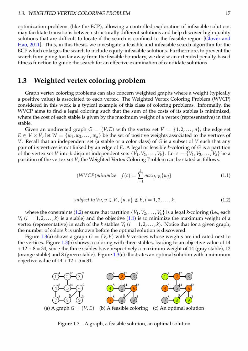
Graph vertex coloring problems can also concern weighted graphs where a weight (typicallya positive value) is associated to each vertex. The Weighted Vertex Coloring Problem (WVCP)considered in this work is a typical example of this class of coloring problems. Informally, theWVCP aims to find a legal coloring such that the sum of the costs of its stables is minimized,where the cost of each stable is given by the maximum weight of a vertex (representative) in thatstable.
Given an undirected graph G = (V, E) with the vertex set V = 1, 2, . . . , n, the edge setE ∈ V × V, let W = w1, w2, . . . , wn be the set of positive weights associated to the vertices ofV. Recall that an independent set (a stable or a color class) of G is a subset of V such that anypair of its vertices is not linked by an edge of E. A legal or feasible k-coloring of G is a partitionof the vertex set V into k disjoint independent sets V1, V2, . . . , Vk. Let s = V1, V2, . . . , Vk be apartition of the vertex set V, the Weighted Vertex Coloring Problem can be stated as follows.
(WVCP)minimize f (s) =k
∑i=1
maxj∈Viwj (1.1)
subject to ∀u, v ∈ Vi, u, v /∈ E, i = 1, 2, . . . , k (1.2)
where the constraints (1.2) ensure that partition V1, V2, . . . , Vk is a legal k-coloring (i.e., eachVi (i = 1, 2, . . . , k) is a stable) and the objective (1.1) is to minimize the maximum weight of avertex (representative) in each of the k stables Vi (i = 1, 2, . . . , k). Notice that for a given graph,the number of colors k is unknown before the optimal solution is discovered.
Figure 1.3(a) shows a graph G = (V, E) with 9 vertices whose weights are indicated next tothe vertices. Figure 1.3(b) shows a coloring with three stables, leading to an objective value of 14+ 12 + 8 = 34, since the three stables have respectively a maximum weight of 14 (gray stable), 12(orange stable) and 8 (green stable). Figure 1.3(c) illustrates an optimal solution with a minimumobjective value of 14 + 12 + 5 = 31.
14
212
39
48
514
612
78
85
93
14
212
39
48
514
612
78
85
93
14
212
39
48
514
612
78
85
93
(a) A graph G = (V, E) (b) A feasible coloring (c) An optimal solution
Figure 1.3 – A graph, a feasible solution, an optimal solution

18 CHAPTER 1. INTRODUCTION
One notices that an instance of the NP-hard vertex coloring problem can be conveniently re-duced to an instance of the WVCP by defining a weight of 1 for each vertex. As a result, theWVCP is NP-hard [Malaguti, 2009; Michael and David, 1979], and thus computationally chal-lenging in the general case. From a practical perspective, the WVCP has a number of practicalapplications in different fields and arises naturally in the context of buffer management in operat-ing systems [Prais and Ribeiro, 2000; Ribeiro et al., 1989], batch scheduling [Gavranovic and Finke,2000] and manufacturing [Hochbaum and Landy, 1997]. As a result, effective solution methodsfor the WVCP can help to solve these practical problems.
1.3.1 Exact approaches
From a perspective of solution methods for the WVCP in the general case, several exact algo-rithms have been proposed.
Specifically, a column generation approach combined with the general branch-and-boundmethod was investigated in [Ribeiro et al., 1989]. Extensive computational experiments were re-ported for the matrix decomposition problem encountered in satellite switching systems, showingthe effectiveness of this approach.
A branch-and-price approach based on column generation was presented in [Furini and Malaguti,2012] and computational results were shown on a subset of benchmark instances from the DI-MACS and COLOR competitions and two sets of instances from matrix-decomposition problems,which shows excellent performances when compared with the best heuristic algorithms from theliterature.
In [Cornaz et al., 2017], the WVCP was solved as Maximum Weight Stable Set Problems on anassociated graph and this approach showed excellent results on the tested benchmark graphs.
The above review indicates that despite the theoretical and practical significance of the WVCP,solution methods for the problem are quite limited and the WVCP benchmark instances are ofsmall sizes in comparison with those used for other graph coloring problems.
1.3.2 Heuristic approaches
Given that the WVCP is a NP-hard problem, several heuristic algorithms have also been inves-tigated, which aim to provide high-quality solutions in acceptable computation time, but withoutprovable optimal guarantee of the attained solutions.
For example, a Greedy Randomized Adaptive Search Procedure (GRASP) was introduced in[Prais and Ribeiro, 2000] in the context of a practical problem called TDMA traffic assignment(an application of the WVCP). This algorithm iterates a mixed search strategy combining a ran-domized greedy construction procedure followed by a local optimization procedure. Extensivecomputational experiments indicate that the Reactive GRASP heuristic matches the optimal solu-tion found by an exact column generation based branch-and-bound algorithm.
In [Malaguti et al., 2009], an effective 2_Phase algorithm was proposed, where in the first phasea large number of independent sets is heuristically produced, and in the second phase the setcovering problem associated with these sets is solved by the Lagrangian heuristic algorithm in-troduced previously in [Caprara et al., 1999]. These heuristics have reported interesting resultson a number of benchmark instances. However, one notices that these methods only examinefeasible solutions.
1.3.3 Summary
Our literature review given in Section 1.3.1 and 1.3.2 indicates that unlike the popular vertexcoloring problem for which numerous solution methods are available (see the reviews [Galinier

1.4. K-VERTEX CRITICAL SUBGRAPHS PROBLEM 19
and Hertz, 2006; Malaguti and Toth, 2010; Galinier et al., 2013]), research on algorithms for theWVCP is still in its infancy with very few advanced methods.
In this work, we aim to fill the gap by investigating effective heuristics that can be used to findhigh-quality approximate solutions for problem instances that cannot be solved exactly.
Our interest on heuristics for the WVCP is fully motivated by the hardness of the consideredproblem. Indeed, unless P =NP , exact algorithms for the WVCP will inevitably have an exponen-tial time complexity and can only be applied to solve problem instances of limited sizes or withparticular features.
Our work focuses on investigating a feasible and infeasible search procedure and is drivenby the following consideration. The WVCP is a constrained combinatorial optimization prob-lem where a feasible solution must satisfy the coloring constraint (i.e., two adjacent vertices mustreceive different colors). Due to the presence of the coloring constraint, the feasible region canbe broken into several zones which are separated from each other by infeasible regions in thesearch space. In this case, an algorithm searching only feasible solutions could be blocked in aparticular feasible zone, thus miss the global optima or high quality solutions located in otherfeasible zones. On the other hand, as illustrated in numerous studies on constrained optimiza-tion, e.g., [Chen et al., 2016b; Glover and Hao, 2011; Jin and Hao, 2016; Lai et al., 2018; Lin, 2013;Martinez-Gavara et al., 2017; Sun et al., 2017; Wang et al., 2018], methods that are allowed to os-cillate between feasible and infeasible regions constitute an appropriate means to cope with sucha situation. Indeed, allowing a controlled exploration of infeasible solutions may facilitate tran-sitions between structurally different solutions and help discover high-quality solutions that aredifficult to locate if the search is limited to the feasible region. Based on previous studies of ex-amining feasible and infeasible solutions for solving other constrained optimization problems,we present in this thesis the first study that mixes both feasible and infeasible searches with thecontext of the WVCP.
1.4 k-vertex critical subgraphs problem
1.4.1 Problem Introduction
A graph is a vertex-critical graph if removing any vertex from the graph decreases its chro-matic number [Desrosiers et al., 2008]. Given an integer k, a k-vertex-critical subgraph (k-VCS) ofG is a vertex-critical subgraph H such that χ(H) = k. Note that each graph G contains at least onek-VCS for 1 ≤ k ≤ χ(G). Finally, a subgraph H∗ is a minimum k-VCS if no other k-vertex-criticalsubgraph with fewer vertices than in H∗ exists in G. The k-VCS problem (k-VCSP) is to find aminimum k-vertex-critical subgraph of G. The k-VCSP is a NP-hard problem and thus computa-tionally challenging [Desrosiers et al., 2008]. For simplicity, if H = (A, EA) is a k-VCS, we alsouse its vertex set A to denote the k-VCS.
The k-VCS problem has important theoretical significance and large application potential. Forinstance, The k-VCS problem helps to find lower bounds on the chromatic number of these graphsand identify hard or unsolvable subproblems that help the tractability of satisfiability testing ofthe real world applications [Herrmann and Hertz, 2002; Hu et al., 2011].
As an example, consider the graph G of Figure 1.4(a) with χ(G) = 4. Figure 1.4(b) showsa 4-vertex-critical subgraph of G since removing any vertex decreases its chromatic number to3. Moreover, this 4-VCS is also minimum since no other 4-critical subgraph can be found in G.Note that k-VCS of G provides a means of determining lower bounds of χ(G), and a k-VCS witha larger k thus leads to a better (tighter) bound (eg., the 4-VCS of Figure 1.4(b) corresponds to abetter lower bound with respect to any 3-VCS formed by a clique of size 3 like 1,2,7).

20 CHAPTER 1. INTRODUCTION
9
8
5 6
1110
3
9
2
7
4
12
1
(a) A graph with chromatic number of 4
1
5
4 3
7
6
2
(b) A 4-vertex-critical subgraph
Figure 1.4 – An example for the 4-vertex-critical subgraph.
1.4.2 Exact approaches
In [Herrmann and Hertz, 2002], Herrmann and Hertz suggested a vertex removal algorithmcombined with an insertion algorithm to find the chromatic number of a graph. Computationalexperiments on random graphs and on DIMACS benchmark problems demonstrate that the pro-posed algorithm can solve larger problems than previous known exact methods.
1.4.3 Heuristic approaches
In the context of graph coloring, some approaches have been proposed to extract k-VCS in agraph.
[Eisenberg and Faltings, 2003] presented two breakout algorithms to identify hard and un-solvable subgraph in a graph. The first approach uses the breakout with backtracking (BOBT)algorithm to solve constraint satisfaction problems or identify an unsolvable subproblem if it ex-ists, the second algorithm is the breakout with backtracking for a smallest unsolvable subproblem(BOBT-SUSP) that identifies a k-VCS. Evaluated on randomly generated graph 3-coloring prob-lems, the proposed algorithm is demonstrated to be highly effective in discovering high qualitysolutions.
[Desrosiers et al., 2008] proposed the neighborhood weight heuristic algorithm that is com-bined with classical critical subgraph detection algorithms, leading to several effective k-VCSdetection heuristics including the Ins + h algorithm. Computational experiments are reported onrandom and DIMACS benchmark graphs to compare the proposed algorithms, as well as to findlower bounds on the chromatic number of these graphs. Computational testing shows that thisalgorithm improves the best known lower bound for some of these graphs and is even able todetermine the chromatic number of some graphs for which only bounds were known previously.
1.4.4 Summary
Although many exact algorithms have been devised for the graph coloring, they can onlybe used to solve small instances. Heuristics coloring algorithms can be used on much largerinstances, but only to get an upper bound on the chromatic number χ(G). Given that the removalstrategy is quite effective for this problem, the last work of this thesis is to design a removalstrategy with a backtracking mechanism and a perturbation procedure to solve the k-VCS in anefficient way.

2A reduction-based memetic algorithm forGCP
In this chapter, we investigate a reduction-based memetic algorithm (RMA) to find a graphcoloring solution for a given graph G. Graph coloring is one of the most studied NP-completeproblems. Given a graph G = (V, E), the task is to partition the vertex set V into k disjoint sub-sets, such that no edge has endpoints in the same subsets. In this work, we present a memeticalgorithm, which integrates a backbone-based coarsening operator (to preserve common infor-mation and reduce the size of graph), a weighted tabu search procedure (to improves the qualityof the solution of the reduced graph) and a perturbation procedure (to escape from the region ofthe local optimum). Extensive experimental studies on numerous benchmark instances from thegraph coloring problem show that the proposed approach, performs equally well as some bestexisting graph algorithms in terms of solution quality.
Contents2.1 Introduction . . . . . . . . . . . . . . . . . . . . . . . . . . . . . . . . . . . . . . . . . 232.2 Memetic algorithm for the GCP . . . . . . . . . . . . . . . . . . . . . . . . . . . . . 23
2.2.1 General approach . . . . . . . . . . . . . . . . . . . . . . . . . . . . . . . . . . 232.2.2 Population initialization . . . . . . . . . . . . . . . . . . . . . . . . . . . . . . 242.2.3 The adaptive multi-parent crossover procedure . . . . . . . . . . . . . . . . 272.2.4 Backbone-based group matching . . . . . . . . . . . . . . . . . . . . . . . . . 272.2.5 Weight tabu search improvement . . . . . . . . . . . . . . . . . . . . . . . . . 302.2.6 Uncoarsening phase . . . . . . . . . . . . . . . . . . . . . . . . . . . . . . . . 312.2.7 Pool updating strategy . . . . . . . . . . . . . . . . . . . . . . . . . . . . . . . 32
2.3 Experimental results and comparisons . . . . . . . . . . . . . . . . . . . . . . . . . 322.3.1 Benchmark instances . . . . . . . . . . . . . . . . . . . . . . . . . . . . . . . . 332.3.2 Experiment settings . . . . . . . . . . . . . . . . . . . . . . . . . . . . . . . . 332.3.3 Comparison with state-of-the-art algorithms . . . . . . . . . . . . . . . . . . 352.3.4 Comparative results on easy instances . . . . . . . . . . . . . . . . . . . . . . 352.3.5 Comparative results on difficult instances . . . . . . . . . . . . . . . . . . . . 36
2.4 Analysis . . . . . . . . . . . . . . . . . . . . . . . . . . . . . . . . . . . . . . . . . . . 372.4.1 Effectiveness of the number of parents for RMA . . . . . . . . . . . . . . . . 372.4.2 Effectiveness of the different matching strategies for RMA . . . . . . . . . . 37
21

22 CHAPTER 2. A REDUCTION-BASED MEMETIC ALGORITHM FOR GCP
2.4.3 Effectiveness of the perturbation operation . . . . . . . . . . . . . . . . . . . 382.5 Conclusions . . . . . . . . . . . . . . . . . . . . . . . . . . . . . . . . . . . . . . . . . 38

2.1. INTRODUCTION 23
2.1 Introduction
Given a simple undirected graph G = (V, E) with vertex set V = 1, 2, . . . , n and edge setE ⊂ V × V, a legal k-coloring of G is a mapping c : V → 1, . . . , k, such that c(i) 6= c(j) forall edges (i, j) in E. The graph k-coloring problem (k-GCP) is to determine if a legal k-coloringof G exists for a given k. The classical graph coloring problem (GCP) is to find the minimuminteger k (chromatic number χ(G)) for which a legal k-coloring of G exists. k-GCP is known to beNP-complete while the optimization problem GCP is NP-hard [Garey and Johnson, 1979].
Since memetic algorithms have been proved to be very effective for solving coloring problems[Galinier and Hao, 1999; Porumbel et al., 2010; Lü and Hao, 2010; Malaguti et al., 2008; Moalicand Gondran, 2015], in this chapter, we introduce the Reduction-based Memetic Algorithm thatintegrates the idea of multilevel optimization [Benlic and Hao, 2011; Walshaw, 2004] within thememetic search framework.
In this work, we adopt for the first time the idea of reduction in a memetic algorithm for theGCP. For this purpose, we address three relevant issues which are critical to make our approachsuccessful. First, we need to identify the previous common information of the parents which iscontained in high quality solutions. Second, we want to reduce the original graph to a smallergraph through the common information, i.e., common fragment showed in the parents can bemerged into one vertex. Third, we wish to search effectively the reduced graph. RMA uses abackbone-based group matching mechanism for identifying common information of the parents.By incorporating this mechanism, RMA merges identical information fragment (with at least twovertices) to form one vertex. The weighted tabu search algorithm examines the reduced graph tofurther improve the solution.
Computational results on 39 benchmark graphs from the DIMACS and COLOR competitionsshow that RMA competes favorably with state-of-the-art algorithms in the literature in termsof solution quality. Specifically, RMA obtains the best-know results for 19 easy instances withan improvement of the computation time and matches the best-known results for 13 difficultinstances.
The rest of the chapter is organized as follows. Section 2.2 describes the proposed algorithmin detail. Section 2.3 presents computational results and comparisons with state of the art al-gorithms. Section 2.4 analyzes the impact of some key components of the proposed algorithm.Conclusions and future work are discussed in the last section.
2.2 Memetic algorithm for the GCP
The conventional GCP can be approximated by finding a series of legal k-colorings for de-creasing k values[Galinier and Hertz, 2006; Galinier et al., 2013]. This process is repeated untilno legal k-coloring can be found. Therefore, we will only consider the k-coloring problem in therest of this section. To seek a legal k-coloring for a given k, we adopt the memetic search whichis a powerful framework that promotes the idea of combining evolutionary computing and localoptimization.
In this section, we propose a way of collapsing vertices based on common information and theresulting RMA algorithm for solving k-GCP.
2.2.1 General approach
As shown in Algorithm 2.1, RMA starts from an initial solution Si generated by the greedyprocedure and further ameliorated by the iterated tabu search procedure described in Section2.2.2. The initialization process repeats p times in order to generate the parent solutions (lines

24 CHAPTER 2. A REDUCTION-BASED MEMETIC ALGORITHM FOR GCP
Algorithm 2.1: The RMA algorithm for solving the k-GCP1: Input: Graph G = (V, E), number of colors k, population size p.2: Output: the best k-coloring S∗ found so far3: for i = 1, 2, . . . , N do4: wi ← 1/ * Initialize the weight of each edge */5: end for6: for i = 1, 2, . . . , p do7: S0 ← Greedy_Initial(G, k) /*Greedy Initialization, Section 2.2.2 */8: Si ← Tabu_Search(G, S0, k) /* Tabu search, Section 2.2.2 */9: Sbest ← Si /*Record the best legal solution at each loop */
10: end for11: S∗ ← arg minF(Si), i = 1, 2, . . . , p /* Record the best solution S∗ found so far*/12: while stop condition met do13: S0 ← Adaptive_MultiParent_Crossover /*Initialize offspring solution S0, Section 2.2.3*/14: Randomly choose 2 individuals solution Sm, Sn f rom parents set P15: (G
′, S0′, w)← Backbone_Coarsening_Operator(Sm, Sn, G, S0) /* Section 2.2.4*/
16: S′best ←Weighted_Tabu_Search(G
′, S′0, k, w) /*Section 2.2.5*/
17: (G, Sc)← Uncoarsening_Perturbation(G′, Sbest
′) /* Section 2.2.6*/18: Sbest ← Tabu_Search(G, Sc, k) /* Future improve the solution, Section 2.2.6*/19: if f (Sbest) < f (S∗) then20: S∗ ← Sbest21: end if22: S1, S2, . . . , Sp ← Pool_Updating(Sbest, S1, . . . , Sp) /*Section 2.2.7*/23: end while
6-10). After initializing the global variable best solution S∗ found so far (line 11), the search entersinto the evolution loop. It repeats an evolution process to improve the population until a prede-fined stopping condition (typically a fixed number of generations) is verified or a legal coloringis found. At each generation, the algorithm randomly selects two parent solutions Sm, Sn fromthe population. Then, we obtain a coarsening graph G
′from G with its corresponding coloring
S0′ and the weight set w by using a backbone coarsening operator (line 15, Section 2.2.4). This
coarsening phase is followed by a weighted tabu search in order to improve the solution (line 16,Section 2.2.5). The uncorsening phase, which recovers the initial graph G from G
′with its cor-
responding coloring, uses a slight perturbation of the corresponding coloring to escape from thelocal optimal solution (line 17, Section 2.2.6). This newly generated coloring is further improvedby the iterated tabu search process (line 18, Section 2.2.6). Finally, a quality-and-distance basedrule is applied to decide if the improved solution can be inserted into the population (line 22,Section 2.2.7).
In the remainder of this section, we explain the main components of the proposed RMA al-gorithm: the initial population generator, the iterated tabu search procedure, the backbone-basedcoarsening operator, the weighted tabu search process and the population updating strategy.
2.2.2 Population initialization
The purpose of the initialization step is to generate an initial coloring with as few conflictsas possible for the given k-GCP problem. This is achieved by two steps: the greedy algorithmproposed in [Glover et al., 1996] and the tabu search in [Galinier and Hao, 1999].

2.2. MEMETIC ALGORITHM FOR THE GCP 25
Begin
Initialization generated p parents
Parent pooling (S1 , . . . , Sp)
Random select NUM solutions Rondom selection Sm Rondom selection Sn
AMPax crossover Backbone based group matching
Reduction Coarsening phase
Weight tabu search improvement
Uncoarsening phase+perturbation
Tabu search improvement
Pool update
Reach the time limit?
Stop
Offspring solution S0
Coarsened solution S′0
Coarsened graph G′= (V
′, E′)
S′best
Sc
Sbest
No
Yes
Figure 2.1 – Flow chart of RMA algorithm for solving the k-GCP.
Greedy initialization
RMA constructs an initial solution according to the greedy constructive heuristic (called DAN-GER), which was first proposed in [Glover et al., 1996], and subsequently was used in severalstudies [Lü and Hao, 2010].
To create each individual of the initial population, we assign a vertex from the set of unas-signed vertices a color class at one time. Specifically, we firstly use a scoring function accordingto the dynamic vertex danger measure to score the unassigned vertices. Given these scores, anunallocated vertex with the highest score is probabilistically selected. Next, the scores of the col-ors for the selected vertex are calculated according to the possibility that this colors are requiredby neighboring vertices. Finally, a color is choosen probabilistically. This process is repeated untilall vertices are assigned a color.
Afterwards, in order to further optimize the solution constructed by the DANGER procedure,we apply an iterated tabu search (Section 2.2.2), previously presented in [Galinier and Hao, 1999].The refinement step is essential for our approach to improve progressively the quality of the initialsolution, which also helps the memetic algorithm to save some computational efforts during thefirst generations of its search. This initialization procedure is iterated until the population is filled

26 CHAPTER 2. A REDUCTION-BASED MEMETIC ALGORITHM FOR GCP
with p (population size) individuals (Algorithm 2.1, lines 6-10).
The iterated tabu search
(1) Search space and fitness functionBefore presenting the ingredients of the tabu search process, we first define the search space
Ωk explored by the algorithm, the evaluation function f (s) to measure the quality of a candidatesolution and the solution representation used by the RMA algorithm.
For a given graph G = (V, E) with k available colors, the search space Ωk visited by RMA iscomposed of all allocations of vertices to the k color class. In other words, the RMA algorithmvisits all the k-colorings. Then the search space is given by:
Ωk = V1, V2, · · · , Vk : ∪ki=1Vi = V, Vi ∩Vj = ∅ (2.1)
where i 6= j, 1 ≤ i, j ≤ k.A candidate solution in Ωk can be represented by s = V1, V2, . . . , Vk such that Vi is the group
of vertices receiving the same color i. For any candidate solution s ∈ Ωk, its quality is evaluateddirectly by the fitness function f (s), which is used to count the conflicting edges induced by s.
f (s) =k
∑i=1|C(Vi)| (2.2)
where C(Vi) is the set of conflicting edges in color class Vi. Accordingly, a coloring s with f (s) = 0corresponds to a legal k-coloring. The objective of RMA is to minimize f , i.e., the number ofconflicting edges to find a legal k-coloring in the search space.
(2) Move operators to explore the space ΩkOne of the most critical features of local search is the definition of its neighborhood. Typi-
cally, a neighborhoods is defined by a move operator which transforms a current solution s =V1, V2, . . . , Vk to generate a neighboring solution by some local changes of s. To explore thesearch space Ωk, the search phase employs one basic move operator to generate neighboring so-lutions which displaces a conflicting vertex v from its current color class Vi to another color classVj. The neighborhood N(s) induced by this operator is given by:
N(s) = s ⊕ < v, Vi, Vj >: v ∈ Vi ∩ C(s), 1 ≤ i, j ≤ k, i 6= j (2.3)
where C(s) denotes the set of conflicting vertices of s, i.e., the vertices involved in a conflictingedge.
Clearly N(s) is bounded by O(|C(s)| × k) in size. To effectively calculate the move gain thatidentifies the change in the fitness function f (Equation (2.2)), we adopt the fast incremental eval-uation technique of [Dorne and Hao, 1999; Fleurent and Ferland, 1996; Galinier and Hao, 1999].The main idea is to maintain a matrix A of size n× k with elements A[v][q] recording the numberof vertices adjacent to v in color class Vq (1 ≤ q ≤ k). Then, the gain of each one-move in terms offitness variation can be efficiently calculated as
∆ f = A[v][j]− A[v][i] (2.4)
Each time a one-move operation involving the vertex v is performed, we just need to update asubset of values affected by this move as follows. For each vertex u adjacent to vertex v, A[u][i]←A[u][i]− 1, and A[u][j]← A[u][j] + 1.

2.2. MEMETIC ALGORITHM FOR THE GCP 27
2.2.3 The adaptive multi-parent crossover procedure
The AMPaX operator is proposed in [Lü and Hao, 2010] which builds one by one the colorclasses of the offspring. Firstly, we chose NUM = 2 + rand()%4 parents for the population pool.Each time the color class with the maximal cardinality in all NUM parent individuals is chosen,in order to transmit as more vertices as possible such that the number of unassigned vertices afterk transmitting steps is as small as possible. After one color class has been assigned, all the verticesin this color class are removed from all parents. This process is repeated until all k color classesare built. At the end of these k steps, some vertices may remain unallocated. These vertices arerandomly assigned to a color class. Thus, offspring solution S0 is constructed.
This crossover step of creating an offspring solution S0 is essential for our approach, whichhelps the weight coloring algorithm to improve progressively the quality of the initial solutionand saves some computational efforts during its search (Section 2.2.5).
2.2.4 Backbone-based group matching
Algorithm 2.2: The backbone-based collapsing algorithm1: Input: two parent solutions Sm = Vm
1 , Vm2 , . . . , Vm
k and Sn = Vn1 , Vn
2 , . . . , Vnk .
2: Output: a matching scheme J3: J ← ∅
/*Match the set of the vertices*/4: Let H = (Vm
i , Vnj ) | i ∈ k, j ∈ k denote the set o f all k× k group combinations o f Sm and Sn.
5: Compute the number o f common vertices f or each group combination (Vmi , Vn
j ) ∈ H6: repeat7: Choose the combination (Vm
i , Vnj ) with the largest ωVm
i ,Vnj
f rom H8: J ← J ∪ (Vm
i , Vnj )
9: H ← H \ (Vmi , Vn
j )10: Remove f rom E all combinations associated with Vm
i and Vnj
11: until H = ∅
Our backbone-based coarsening operator is composed of two steps: backbone-based groupmatching and coarsening phase, whose components are detailed in the following sections.
We introduce the following basic definitions which are helpful for the description of the pro-posed approach. Let Sm = Vm
0 , Vm1 , ..., Vm
k and Sn = Vn0 , Vn
1 , ..., Vnk be two parent solutions
respectively.
Definition 2.2.1. The set of common objects H denotes tthe set of common objects that has identicalobject grouping of Sm and Sn , i.e., H = (Vm
i , Vnj )|i ∈ k, j ∈ k denote the set of all k ∗ k group
combinations o f Sm and Sn.
Definition 2.2.2. The Backbone matching set J = (Vmi , Vn
j ), 1 ≤ i, j ≤ k denotes the largest setof common objects for each color of two parents Sm and Sn. We apply a fast greedy algorithm toseek a near-optimal backbone matching.
At the first step, the algorithm randomly selects two parent solutions Sm, Sn from the pop-ulation and matches them by using a backbone-based group matching operator, thus gets thematching scheme J. According to the identical information set, we merge each identical informa-tion fragment Ii = Vi ∩Vj, (Vm
i , Vnj ) ∈ J, 1 ≤ i, j ≤ k to one coarsened vertex which ends up with
the coarsening graph G′
(see Figure 2.4 for an illustrative example).

28 CHAPTER 2. A REDUCTION-BASED MEMETIC ALGORITHM FOR GCP
Backbone-based group matching
Apart from the local optimization procedure, group matching is another key component forour RMA algorithm. A successful group matching operator should be able to transmit the mean-ingful features from parents to offspring and offer some diversity.
As described in Section 2.1, a solution can be regarded as a partition of N vertices into k classes.It is more significant to manipulate classes of vertices than individual vertex when transmittinguseful information.
Preliminary experiments show that high quality local optimal solutions share many groupingvertices. It is thus expected that vertices that always share the same color are very likely to bepart of a global optimum or a high quality solution. Following this observation, the general ideaof our proposed collapsing operator is to preserve the vertices groupings (backbone) of maximalsize from parent solutions and color the rest vertices randomly.
Sm Vm1 Vm
2. . . Vm
i. . . Vm
k
Sn Vn1 Vn
2. . . Vn
j . . . Vnk
(a) A complete bipartite graph H with an edge weight ω
Sm Vm1
ωVmi ,Vn
2
Vm2
. . . Vmi
. . . Vmk
Sn Vn1 Vn
2. . . Vn
j . . . Vnk
(b) Choose an edge with the largest ω and delete all edges incident to vertices
Sm Vm1
ωVm2 ,Vn
1
Vm2
. . . Vmk
Sn Vn1
. . . Vnj . . . Vn
k
(c) Repeat the last step until H = ∅
Figure 2.2 – The classes matching procedure by a complete bipartite graph H
Each vertex set (or color class) Vmi from parent solution Sm that shares the most common
vertices typically corresponds to another set Vnj of parent solution Sn. Therefore, in order to find
out the largest number of common vertices of two parent solutions, the first step is to match eachset in two parents.
This is achieved by finding a maximum weight matching in a complete bipartite graph H =(VH , EH) (Figure 2.2(a)) where VH consists of k upside vertices and k downside vertices that cor-respond respectively to the vertex sets of parent solutions Sm and Sn; each edge (Vm
i , Vnj ) ∈ H
is associated with a weight ωVmi ,Vn
j, which is defined as the number of identical vertices in Vm
i of

2.2. MEMETIC ALGORITHM FOR THE GCP 29
solution Sm and Vnj of solution Sn.
The maximum weight matching problem can be solved by using the classical Hungarian al-gorithm [Kuhn, 1955]. However, invoking this algorithm for each iteration would be too com-putationally expensive (O(k3)). We apply a fast greedy algorithm [Chen and Hao, 2016] to seeka near-optimal weight matching for the maximum weight matching problem. The main idea isthat at each step our greedy algorithm chooses an edge (Vm
i , Vnj ) ∈ H with the largest ωVm
i ,Vnj
,keep this set (Vm
i , Vnj ) in the group matching set J, i.e., J ← J ∪ (Vm
i , Vnj ) and delete it from the
graph H (H ← H \ (Vmi , Vn
j )). All edges incident to vertex Vmi and to vertex Vn
j are also deletedin order to make it easier to identify the next match set, as showed in the Figure 2.2(b)-(c). Thisprocedure is repeated until H becomes empty (lines 4-11 of Algorithm 2.2), which occurs whenall vertex sets are matched.
To illustrate the main steps of the backbone-based matching operator, we use the case of Fig-ure 2.3 as a working example. The example involves an instance of 5 vertices and 3 colors andoperates with two parent solutions Sm and Sn. In the first step, as showed in Figure 2.3, Sm andSn are matched using the fast greedy algorithm and the results are: Sm-Vm
1 matches Sn-Vn1 , Sm-Vm
2matches Sn-Vn
3 (randomly choice between Sm-Vm3 and Sn-Vn
2 for equal weight) and the matchingset J = (Vm
1 , Vn1 ), (V
m2 , Vn
3 ), (Vm4 , Vn
2 ) .
1
2
3
45
Sm
1
2
3
45
Sn
Sm
Vm1 Vm
2 Vm3
14
25
3
Sn
Vn1 Vn
2 Vn3
14
23
5
(a) Sm and Sn for a graph G = (V, E) (b) An example of classes matching
Figure 2.3 – two solutions for a graph coloring and its graph matching G′
Algorithm 2.3: The coarsening phase1: Input: Matching set J.2: Output: the coarsener graph G
′
3: G′ ← G/* Initial the coarsener graph G
′*/
4: for each set (Vi, Vj) ∈ J do5: Ii ← Vi ∩ Vj /∗Ii is the ith identical information fragment∗/6: Collapse all vertices in the set Ii to form one vertex in the graph G
′
7: Update the weight of the edges in the graph G′
8: end for

30 CHAPTER 2. A REDUCTION-BASED MEMETIC ALGORITHM FOR GCP
Coarsening phase
Let G = (V, E) be the initial graph. Creating a coarsened graph G′= (V
′, E′) from G consists
of finding an identical information set, merging each identical information fragment and thencollapsing those sets to one vertex to form a new vertex in G
′. Any vertex that dose not belong to
any fragment is simply copied to G′.
The proposed coarsening phase is illustrated in Algorithm 2.3. Firstly, let the initial graphG′
as G and the edge weight of G be initialized to 1 (line 3, Algorithm 2.3). Then, we collapsethe identical vertices from parent solutions which are recorded in the backbone matching set J toform one vertex (line 5-6, Algorithm 2.3). Finally, we update the weight of each edge of G
′(line
7, Algorithm 2.3). To be specific, the weight of each edge of a coarsened graph G′
equals the sumof weights of the edges of the initial graph whose endpoints respectively belong to the vertices ofthis edge of the coarsened graph. Therefore, the sum of the weights of the edges of the coarsenedgraph equals the number of the edges of the initial graph G. Repeat this process until all theidentical vertices are collapsed.
1
2
3
45
Sm1
11
1
1
1
1
1
2
3
45
Sn1
11
1
1
1
1
1v′1 = v1, v4 1
21
2
12
3
5
(a) Sm and Sn for a graph G = (V, E) (b) A coarsened graph G′
Figure 2.4 – two solution for a graph coloring and its coarsened graph G′
An example of the coarsened graph G′
of an initial graph G with 5 vertices is provided inFigure 2.4. Let v
′1 of G
′be vertex formed by collapsing v1, v4 of G. These edges between v1, v4
and the vertices incident to vertices and v1, v4 in the initial graph G are merged to form a newedge with a weight that is set equal to the sum of the weights of the edges whose endpoints areincident to v1 or v4, .i.e., W
′1,5 = W1,5 + W4,5 = 2, W
′1,3 = W1,3 + W4,3 = 2.
After coarsening the original graph G to G′, we apply a weighted tabu search to improve the
solution in the graph G′(see the Section 2.2.5). Normally, the quality of a solution for the graph
G′
is worse than that of G because there is a less degree of freedom for refinement. However, thisphase helps the search quickly attain a promising search area.
2.2.5 Weight tabu search improvement
Recall that the purpose of the backbone based group matching phase is to obtain a coarsenedgraph G
′. In order to find a good initial solution S
′0 for the graph G
′, we simplify the solution
S0 (which is generated by the adaptive multi-parent crossover procedure), which means that if avertex is merged with another vertex, the color of this vertex is deleted; otherwise, we keep thecolor of the vertex.
We apply a weighted iterated tabu search algorithm whose basic components are briefly de-scribed in this section. We first define the search space and the evaluation function. For a given

2.2. MEMETIC ALGORITHM FOR THE GCP 31
graph G′= (V
′, E′) with k available colors, the search space contains all possible k-colorings (can-
didate solutions). A candidate solution in Ω′k can be represented by s = V1, V2, . . . , Vk such that
Vi is the set of vertices receiving the same color i.
Ω′k = V1, V2, · · · , Vk : ∪k
i=1Vi = V′, Vi ∩Vj = ∅ (2.5)
where i 6= j, 1 ≤ i, j ≤ k.The evaluation function f
′(s) is used to count the sum of the weight of conflicting edges in-
duced by a coloring s.
f′(s) =
k
∑i=1|w(Vi)| (2.6)
where |w(Vi)| is the weight of conflicting edges in color class Vi. Accordingly, a coloring s withf′(s) = 0 corresponds to a legal k-coloring.
Weighted graph coloring
The used optimization procedure is a version based on the weight of edge of the tabu coloringprocedure (TabuCol) proposed in [Dorne and Hao, 1998; Galinier and Hao, 1999].
Given a conflicting k-coloring solution s = V1, V2, . . . , Vk, the basic idea of the one moveneighborhood N(s) is to move a conflicting vertex v from its original vertices set Vi to anothersubset Vj.
The move gain, which represents the change in the optimization objective, which is expressedas follows
∆ f′= B[v][j]− B[v][i] (2.7)
According to incremental technique, each time a one-move operation involving vertex v isperformed, we just need to update a subset of values affected by this move as follows. For eachvertex u adjacent to vertex v, B[u][i]← B[u][i]− wv,u, and B[u][j]← B[u][j] + wv,u.
Weight TabuCol selects a best neighbor sNbest ∈ N(s) according to the move gain given byEquation 2.7 and the tabu tenure such that either the move gain for the sNbest is the minimum(sNbest is the best solution) not forbidden by the tabu list or is better than the best solution foundso far. If there is more than one vertex with the same move gain, we will choose one vertexrandomly.
2.2.6 Uncoarsening phase
The uncoarsening phase carries out the inverse of the coarsening phase and further improvesthe solution. The details of the underlying steps are described as follows.
(1) Recover the initial graph G from the collapsed graph G′
with its corresponding coloring.As we mentioned, the quality of a solution for the graph G
′is worse than that of G because there
is a less degree of freedom for refinement. Thus, The first step of the uncoarsening phase is torecover from the collapsed graph G
′the original graph G in order to explore the search space
further.(2) Perturbation process. Since our tabu search procedure focuses its search only around con-
flicting vertices, it can get trapped in a local optimum. Therefore, we periodically apply a simple

32 CHAPTER 2. A REDUCTION-BASED MEMETIC ALGORITHM FOR GCP
perturbation before the tabu search process. The perturbation consists of moving a fixed numberof vertices (is set in this chapter to 0.3 ∗ N) in the following way.
This perturbation adopts the one-move operator. To avoid a too strong deterioration of theperturbed solution, a directed perturbation move takes into consideration the fitness value andcannot move back to the original color. While a decent perturbation performs a one-move withoutconsidering the tabu tenure. To combine these two types of perturbations, each type of pertur-bation is determined probabilistically. The resulting solution from the perturbation procedure isthen used as the new starting solution of the next round of the search phase.
After the uncoarsening phase, we run the tabu search (see Section 2.2.2) to further improve thesolution.
2.2.7 Pool updating strategy
Maintaining a healthy diversity of the population is another key issue for population-basedal- gorithms. To decide whether the newly generated solution should be inserted into the pop-ulation or be discarded, we consider not only the solution quality but also the distance betweenindividuals in population. Our algorithm adopts the idea presented in [Lü and Hao, 2010].
Distance measure: Given two k-colorings Sm and Sn, according to the well-known set-theoreticpartition distance [Gusfield, 2002], the distance between Sm and Sn is defined as the minimumnumber of one-move steps needed to transform Sm to Sn, i.e., d(Sm, Sn) = |V| − sim(Sm, Sn),where sim(Sm, Sn) represents the maximum number of elements of Sm that do not need to bedisplaced to obtain the solution Sn.
Di,POP = mindi,j : Sj ∈ POP, j 6= i (2.8)
We use the sim(Sm, Sn) identify the similarity (Sm, Sn) in Section 2.2.4.
Qi,POP = f (Si) + eβ/Di,POP (2.9)
where f represents its fitness in the equation 2.2. and β a parameter set to β = 0.08 ∗ |V|.The pool updating strategy consists thus of three steps: for each individual Si, i ∈ POP,
calculating Di,POP and the corresponding Qi,POP score (lines 5 of Algorithm 2.4); identifying themaximum score Qmax (lines 6 of Algorithm 2.4); and updating the pool (lines 10-15 of Algorithm2.4). This pool updating strategy contributes to avoid premature convergence for population-based algorithms. The pool updating procedure is described in Algorithm 2.4.
2.3 Experimental results and comparisons
This section is dedicated to an experimental assessment of the proposed RMA algorithm forsolving the GCP and comparisons with other state of the art methods. The study is based on39 conventional benchmark instances which are commonly used in the literature and initiallyproposed for the DIMCAS and COLOR competitions for graph coloring problems 1, 2.
1. http://www.dimacs.rutgers.edu/2. http://www.cs.hbg.psu.edu/txn131/graphcoloring.html/

2.3. EXPERIMENTAL RESULTS AND COMPARISONS 33
Algorithm 2.4: Pool updating strategy1: Input: Population POP = S1, S2, . . . , Sp and new solution S0.2: Output: Updated population POP = S1, S2, . . . , Sp
/*Evaluate each solution*/3: Tentatively add S0 to population POP = POP ∪ S04: for i =0,1,. . . ,p do5: Calculate the distance Di,POP between any individual in POP according to the Equation 2.86: Calculate the goodness score Qi,POP according to the Equation 2.97: end for
/*Select the worst solution*/8: Choose the k− coloring with the largest Q value9: Sw ← arg maxQ(Si), i = 0, 1, . . . , p
/*Update the pool population*/10: if Sw 6= S0 then11: Replace Sw with S0 /*Replace the worst solution*/12: else if rand(0, 1) < 0.2 then13: Ssw ← arg maxQ(Si), i = 1, . . . , p14: Replace the orignal pop worst solution Ssw with S0 /*Replace the second worst solution*/15: end if
2.3.1 Benchmark instances
The 33 benchmark instances are classified into two categories: easy graphs and difficult graphsaccording to [Galinier et al., 2013; Galinier et al., 2008]. Let BKV (the best-known value) representsχ(G) (if known) or the best-known value in the literature.
1. The first category, easy graphs, contains 19 instances that can be colored with BKV colors bya basic coloring algorithm like DSATUR [Brélaz, 1979] (thus by numerous algorithms).
2. The second category contains 20 instances that are hard graphs that can only only be achievedby a few advanced coloring algorithms.
2.3.2 Experiment settings
The proposed algorithm was programmed in C++ and compiled by GNU g++ 4.1.2 with -O3flag (option). The experiments were conducted on a computer with an Intel Xeon E5-2670 proces-sor (2.5 GHz and 2 GB RAM) running Ubuntu 12.04. Without using a compiler optimization flag,it requires respectively 0.46, 2.68 and 10.70 seconds to solve the well-known DIMACS machinebenchmark graphs r300.5, r400.5 and r500.5 on our machine.
Parameters
Since our algorithm is built up on the memetic algorithm proposed in [Lü and Hao, 2010],we adopt the parameters in [Lü and Hao, 2010], as the default setting of the RMA algorithm,as shown in Table 2.1. We use the default setting of Table 2.1 to report the experimental resultsshown in the rest of this chapter.
Table 2.1 – Settings of important parameters
Parameters Description Value
p size of population 20β maximum number of iterations for the tabu search methods 10000P0 probability for accepting worse solution 0.2

34 CHAPTER 2. A REDUCTION-BASED MEMETIC ALGORITHM FOR GCP
Reference algorithms
To evaluate the performance of the proposed algorithm, ten state-of-the-art heuristic algo-rithms in the literature are used as the main reference algorithms, including (1) Iterated localsearch algorithm (IGrAl) [Caramia and Dell Olmo, 2008] (a 2.8 GHz Pentium 4 processor and acut off time of 1 hour); (2) Variable space search algorithm (VSS) [Hertz et al., 2008] (a 2.0 GHzPentium 4 processor and a cut off time of 10 hours); (3) Local search algorithm using partial solu-tions (Partial) [Blöchliger and Zufferey, 2008] (a 2.0 GHz Pentium 4 and a time limit of 10 hourstogether with a limit of 2 ∗ 109 iterations without improvement); (4) Probability learning based lo-cal search (PLSCOL) [Zhou et al., 2018] (Intel Xeon E5-2760 2.8 GHz processor and 2 GB RAM witha cutoff of 5 hours); (5) Hybrid evolutionary algorithm (HEA) [Galinier and Hao, 1999] (the pro-cessor used is not available for this oldest algorithm and the results were obtained with differentparameter settings); (6) Adaptive memory algorithm (AMA) [Galinier et al., 2008] (the proces-sor applied is not available and the results were obtained with different parameter settings); (7)Two-phase evolutionary algorithm (MMT) [Malaguti et al., 2008] (a 2.4 GHz Pentium processorand a cut off time of 6000 or 40000 seconds); (8) Evolutionary algorithm with diversity guarantee(Evo-Div) [Porumbel et al., 2010] (a 2.8 GHz Xeon processor and a cut off time of 12 hours); (9)Memetic algorithm (MACOL or MA) [Lü and Hao, 2010] (a 3.4 GHz processor and a cutoff timeof 5 hours); (10) Distributed quantum annealing algorithm (QACOL or QA) [Titiloye and Crispin,2011; Titiloye and Crispin, 2012] (a 3.0 GHz Intel processor with 12 cores and a cut off time of 5hours); (11) The newest parallel memetic algorithm (HEAD) [Moalic and Gondran, 2015] (a 3.1GHz Intel Xeon processor with 4 cores used to run in parallel the search processes with a cut offtime of at least 3 hours).
Stopping condition
Despite the extremely vast literature on graph coloring, there is no uniform experimental stop-ping criteria to assess a coloring algorithm. This is mainly because the difficult DIMACS instancesare really challenging, the best-known solutions for these instances can be found only by few mostpowerful algorithms which were implemented with different programming languages and exe-cuted under various computing platforms and different stopping conditions (maximum allowedgenerations, maximum allowed fitness evaluations, maximum allowed iterations or maximumallowed time limit).
On the other hand, these reference algorithm were tested on different CPU frequency, it wouldbe quite difficult to compare CPU times of the compared algorithms.
To make a relatively fair comparison of the runtime, we use the best solution (i.e., the smallestnumber of used colors) for this comparative study. This experimental conditions of the comparedalgorithms are not equivalent, since the computing time of each algorithm is not only influencedby the processor, but also by some inaccessible factors such as the operating systems, compliers,the comparison is just intended to show the relative performance of the proposed algorithm.
One can observe that the majority of the reference algorithms allowed large run time limitsof at least 5 hours (the cut off limit for our experiments). Additionally, our Intel Xeon E5-26702.5 GHz processor is almost the same with those used by the reference algorithms. Thus, we usethe stopping criterion of 5 hours to investigate the ehavior of our RMA algorithm on the set of 39instances. For each instance, our algorithm was executed 20 times independently. As a result, ouradopted stopping conditions can be considered as reasonable with respect to those used by thereference algorithms.
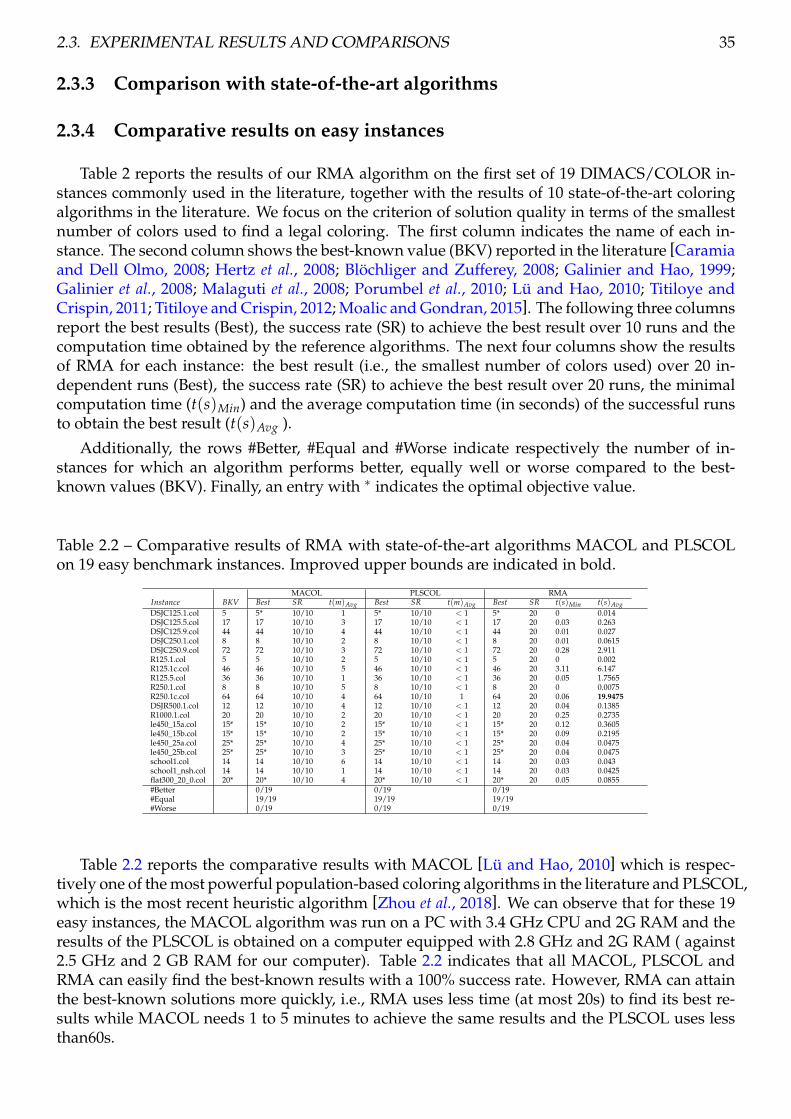
2.3. EXPERIMENTAL RESULTS AND COMPARISONS 35
2.3.3 Comparison with state-of-the-art algorithms
2.3.4 Comparative results on easy instances
Table 2 reports the results of our RMA algorithm on the first set of 19 DIMACS/COLOR in-stances commonly used in the literature, together with the results of 10 state-of-the-art coloringalgorithms in the literature. We focus on the criterion of solution quality in terms of the smallestnumber of colors used to find a legal coloring. The first column indicates the name of each in-stance. The second column shows the best-known value (BKV) reported in the literature [Caramiaand Dell Olmo, 2008; Hertz et al., 2008; Blöchliger and Zufferey, 2008; Galinier and Hao, 1999;Galinier et al., 2008; Malaguti et al., 2008; Porumbel et al., 2010; Lü and Hao, 2010; Titiloye andCrispin, 2011; Titiloye and Crispin, 2012; Moalic and Gondran, 2015]. The following three columnsreport the best results (Best), the success rate (SR) to achieve the best result over 10 runs and thecomputation time obtained by the reference algorithms. The next four columns show the resultsof RMA for each instance: the best result (i.e., the smallest number of colors used) over 20 in-dependent runs (Best), the success rate (SR) to achieve the best result over 20 runs, the minimalcomputation time (t(s)Min) and the average computation time (in seconds) of the successful runsto obtain the best result (t(s)Avg ).
Additionally, the rows #Better, #Equal and #Worse indicate respectively the number of in-stances for which an algorithm performs better, equally well or worse compared to the best-known values (BKV). Finally, an entry with ∗ indicates the optimal objective value.
Table 2.2 – Comparative results of RMA with state-of-the-art algorithms MACOL and PLSCOLon 19 easy benchmark instances. Improved upper bounds are indicated in bold.
Instance BKVMACOL PLSCOL RMA
Best SR t(m)Avg Best SR t(m)Avg Best SR t(s)Min t(s)AvgDSJC125.1.col 5 5* 10/10 1 5* 10/10 < 1 5* 20 0 0.014DSJC125.5.col 17 17 10/10 3 17 10/10 < 1 17 20 0.03 0.263DSJC125.9.col 44 44 10/10 4 44 10/10 < 1 44 20 0.01 0.027DSJC250.1.col 8 8 10/10 2 8 10/10 < 1 8 20 0.01 0.0615DSJC250.9.col 72 72 10/10 3 72 10/10 < 1 72 20 0.28 2.911R125.1.col 5 5 10/10 2 5 10/10 < 1 5 20 0 0.002R125.1c.col 46 46 10/10 5 46 10/10 < 1 46 20 3.11 6.147R125.5.col 36 36 10/10 1 36 10/10 < 1 36 20 0.05 1.7565R250.1.col 8 8 10/10 5 8 10/10 < 1 8 20 0 0.0075R250.1c.col 64 64 10/10 4 64 10/10 1 64 20 0.06 19.9475DSJR500.1.col 12 12 10/10 4 12 10/10 < 1 12 20 0.04 0.1385R1000.1.col 20 20 10/10 2 20 10/10 < 1 20 20 0.25 0.2735le450_15a.col 15* 15* 10/10 2 15* 10/10 < 1 15* 20 0.12 0.3605le450_15b.col 15* 15* 10/10 2 15* 10/10 < 1 15* 20 0.09 0.2195le450_25a.col 25* 25* 10/10 4 25* 10/10 < 1 25* 20 0.04 0.0475le450_25b.col 25* 25* 10/10 3 25* 10/10 < 1 25* 20 0.04 0.0475school1.col 14 14 10/10 6 14 10/10 < 1 14 20 0.03 0.043school1_nsh.col 14 14 10/10 1 14 10/10 < 1 14 20 0.03 0.0425flat300_20_0.col 20* 20* 10/10 4 20* 10/10 < 1 20* 20 0.05 0.0855#Better 0/19 0/19 0/19#Equal 19/19 19/19 19/19#Worse 0/19 0/19 0/19
Table 2.2 reports the comparative results with MACOL [Lü and Hao, 2010] which is respec-tively one of the most powerful population-based coloring algorithms in the literature and PLSCOL,which is the most recent heuristic algorithm [Zhou et al., 2018]. We can observe that for these 19easy instances, the MACOL algorithm was run on a PC with 3.4 GHz CPU and 2G RAM and theresults of the PLSCOL is obtained on a computer equipped with 2.8 GHz and 2G RAM ( against2.5 GHz and 2 GB RAM for our computer). Table 2.2 indicates that all MACOL, PLSCOL andRMA can easily find the best-known results with a 100% success rate. However, RMA can attainthe best-known solutions more quickly, i.e., RMA uses less time (at most 20s) to find its best re-sults while MACOL needs 1 to 5 minutes to achieve the same results and the PLSCOL uses lessthan60s.

36 CHAPTER 2. A REDUCTION-BASED MEMETIC ALGORITHM FOR GCP
2.3.5 Comparative results on difficult instances
Table 2.3 presents the comparative results of RMA with state-of-the-art algorithms on the 20difficult instances. In this table, column 2 recalls the chromatic number or best-known value(BKV) in the literature. The next four columns show the results of the local search algorithm foreach instance. The following 10 columns report the best results obtained by the 4 reference localsearch algorithm and 7 reference population-based algorithms. The last column is the best resultobtained by RMA.
Additionally, in order to show the performance of RMA, we use the rows #Better_compareRMA,#Equal_compareRMA and #Worse_compareRMA to indicate respectively the number of instancesfor which an algorithm performs better, equally well or worse compared to the best-known valuesof RMA (Best). As we observe from Table 2.3, RMA competes favorably with the reference algo-
Table 2.3 – Comparative results of RMA with state-of-the-art algorithms MACOL and PLSCOLon 20 difficult benchmark instances. The best results are in bold.
Instance BKVLocal search algorithms Population-based algorithms
IGrAl VSS Partial PLSCOL HEA AMA MMT Evo-Div MA QA HEAD RMA2008 2008 2008 2018 1999 2008 2008 2010 2010 2011 2015 Best
DSJC250.5.col 28 29 - - 28 - 28 28 - 28 28 28 28DSJC500.1.col 12 12 12 12 12 12 12 12 12 12 12 12 12DSJC500.5.col 47 50 48 48 48 48 48 48 48 48 48 47 48DSJC500.9.col 126 129 126 127 126 126 126 127 126 126 126 126 126DSJC1000.1.col 20 22 20 20 20 20 20 20 20 20 20 20 20DSJC1000.5.col 82 94 86 89 87 83 84 84 83 83 83 82 83DSJC1000.9.col 222 239 224 226 223 224 224 225 223 223 222 222 223DSJR500.1c.col 85 85 85 85 85 - 86 85 85 85 85 85 85DSJR500.5.col 122 126 125 125 126 - 127 122 122 122 122 - 122le450_15c.col 15* 16 15* 15* 15* 15* 15* 15* - 15* 15* - 15*le450_15d.col 15* 16 15* 15* 15* 15* 15* 15* - 15* 15* - 15*le450_25c.col 25* 27 25* 25* 25* 26 26 25* 25* 25* 25* 25* 25*le450_25d.col 25* 27 25* 25* 25* 26 26 25* 25* 25* 25* 25* 25*flat300_26_0.col 26* - - - 26* - 26* 26* - 26* - - 26*flat300 28 0.col 28* - 28* 28* 30 31 31 31 31 29 31 31 29flat1000_76_0.col 81 - 85 87 86 83 84 83 82 82 82 81 83R250.5.col 65* - - 66 66 - - 65 65* 65* 65* 65* 65*R1000.1c.col 98 - - - 98 - - 98 98 98 98 98 98R1000.5.col 234 238 245 238 254 255 - 234 238 245 238 245 254latin_square_10.col 97 100 - - 99 - 104 101 100 99 98 - 98#Better 0/14 0/14 0/16 0/20 0/12 0/17 0/20 0/16 0/20 0/19 0/15 0/20#Equal 2/14 9/14 8/16 11/20 5/12 7/17 13/20 9/16 13/20 13/19 13/15 13/20#Worse 12/14 5/14 8/16 9/20 7/12 10/17 7/20 7/16 7/20 6/19 2/15 7/20#Better_compareRMA 0/14 1/14 2/16 1/20 0/12 0/17 1/20 2/16 2/20 3/19 4/15 -#Equal_compareRMA 2/14 9/14 8/16 13/20 8/12 8/17 14/20 12/16 17/20 15/19 9/15 -#Worse_compareRMA 12/14 4/14 6/16 7/20 4/12 9/17 5/20 2/16 1/20 1/19 1/15 -
rithms. In order to facilitate comparisons, we divide these reference algorithms into three groups.The first group contains 3 algorithm, MA, PLSCOL and MMT, which has the complete experi-mental results for the 20 difficult instances. Observes that RMA attains 13 best known valueswhile PLSCOL, MA and MMT obtains 11, 13 and 13 respectively. RMA, MA and MMT performsimilarly, while the differnce between RMA and PLSCOL is significant.
The second category contains algorithms IGrAI, Partial, HEA, AMA and Evo-Div, which doesnot contain all 20 corresponding resluts. However, RMA competes favorably with those algo-rithm since it can obtain less values in the row of #Worse, which means RMA at least can domi-nate those algorithms. In detail, RMA is worse than BKV for 7 instances out of 20 instances, whileIGrAI, Partial, HEA, AMA, Evo-Div are worse than BKV for 12, 8, 7, 10 and 7 respectively.
The third category cantains the last three algorithms (VSS, QA and HEAD), whose values ofthe row of #Worse are smaller than the value of the row of #Worse of RMA. which also missessome corresponding resluts in the 20 difficulty instances. When comparing RMA with VSS, oneobserves that RMA also performs very well. Specifically, RMA improves the best results of VSSfor 4 instances while matching the best results of RMA for other 9 instances. Only in one case,f lat300_28_0, RMA obtains a slightly worse results. Additionally, when comparing to the bestresults obtained by QA, RMA obtains 3 worse results, 1 better results and matches the remaininginstances. Finally, RMA obtains 5 worse results and 1 better result compared with the results ofHEAD.

2.4. ANALYSIS 37
2.4 Analysis
This section performs additional experiments to gain understanding of some important ingre-dients of the proposed RMA approach: the number of parents for RMA, the strategy of the groupmatching and the perturbation strategy.
2.4.1 Effectiveness of the number of parents for RMA
To assess the influence of the number of parents in the proposed algorithm, we create a algo-rithmic variant (called RMAmutiparents) in which multi-parents are used in the backbone match-ing process ( Section 2.2.4) when collapsing vertices. In detail, those vertices whose colors areidentical should also be allocated to the same color in all chosen parents. For this experiment, weselect 16 instances which are relatively difficult according to the results reported in Tables 2.3.
We ran 10 times both algorithms to solve each selected instance with a cutoff time of 9000seconds (2.5 hour). The comparative results of this experiment are presented in Table 2.4 with thesame information as before.
The rows #Better/#Equal/#Worse indicate the number of instances for which each algorithmattain a better, equal and worse results compared to the other algorithm in terms of the bestobjective value found by RMA.
Table 2.4 reports that RMA dominates the RMAmutiparents algorithm on the 16 instancestested by both algorithm, by obtaining better results for 12 instances and the same results for theremaining 4 instances.
Table 2.4 – Assessment of different number of the parents. The better results are in bold.
Instance BKVRMA RMAmutiparents
Best SR t(s)Min t(s)Avg Best SR t(s)Min t(s)AvgDSJC1000.1.col 20 20 8 1456.91 2919.92 21 10 1.23 8.177DSJC1000.5.col 84 84 4 3140.62 6015.84 88 848.9 4703.63 9DSJC1000.9.col 224 224 9 3073.77 5248.5 226 4937.8 5406.56 2DSJC500.5.col 48 48 10 568 952.641 >48 - - -DSJC500.9.col 126 126 9 356.77 831.989 >126 - - -DSJR500.1c.col 85 85 9 51.52 1439.14 >85 - - -DSJR500.5.col 123 123 4 2568.1 5904.71 127 555.21 3787.49 5flat300_28_0.col 29 29 2 915.63 1109.07 30 3 2382.55 3375.8latin_square_10.col 99 99 6 1818.46 4148.19 >99 - - -le450_15c.col 15 15 10 1471.31 2386.74 15 5 0 2826.1le450_15d.col 15 15 9 1885.01 3457.61 16 10 0.29 6.986le450_25c.col 25 25 4 252.26 4844.03 25 7 1984.45 4842.53le450_25d.col 25 25 5 2106.12 4861.31 25 3 3004.16 6340.4r1000.1c.col 98 98 10 137.6 275.987 98 10 225.45 1767.97R1000.5.col 256 256 3 6672.23 7708.9 >256 - - -R250.5.col 65 65 10 374.91 2273.22 >65 - - -#Better 12/16 0/16#Equals 4/16 4/16#Worse 0/16 12/16
2.4.2 Effectiveness of the different matching strategies for RMA
The group matching procedure (Section 2.2.4) allows the information of the parents to be pre-served during the coarsening process. In this section, we discuss how those group matchingcoarsening processes contribute to the overall performance of our RMA algorithm.
For this study, we create RMA_maxmatch, which is a RMA variant where we replace line15 of Algorithm 2.1 with the group comparison procedure of MACOL. We ran RMA_maxmatchunder the same stopping condition as before in Section 2.4.1 if a legal k-coloring is found or themaximum allowed run time of 2.5 CPU hours is reached. Each tested instance was solved 10times.
Table 2.5 displays the comparative results between RMA and RMA_maxmatch, based onthe same indicators adopted in Table 2.4. From this table, we observe that RMA outperformsRMA_maxmatch, achieving better values for 5 out of 16 instances and equal results for the re-maining 11 instances. Moreover, for the 11 instances where both algorithms achieve the same
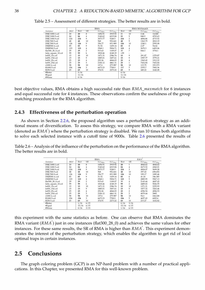
38 CHAPTER 2. A REDUCTION-BASED MEMETIC ALGORITHM FOR GCP
Table 2.5 – Assessment of different strategies. The better results are in bold.
Instance BKVRMA RMA MAXmatch
Best SR t(s)Min t(s)Avg Best SR t(s)Min t(s)AvgDSJC1000.1.col 20 20 8 1456.91 2919.92 21 10 2.46 14.068DSJC1000.5.col 84 84 4 3140.62 6015.84 88 9 848.9 4703.63DSJC1000.9.col 224 224 9 3073.77 5248.5 224 2 4084.86 4715.52DSJC500.5.col 48 48 10 568 952.641 48 9 1363.79 2810.19DSJC500.9.col 126 126 9 356.77 831.989 126 10 1240.1 2592.08DSJR500.1c.col 85 85 9 51.52 1439.14 85 8 2.07 54.64DSJR500.5.col 123 123 4 2568.1 5904.71 123 4 2670.3 6493.06flat300_28_0.col 29 29 2 915.63 1109.07 30 7 844.3 3754.1latin_square_10.col 99 99 6 1818.46 4148.19 >99 - - -le450_15c.col 15 15 10 1471.31 2386.74 15 9 291.87 1370.87le450_15d.col 15 15 9 1885.01 3457.61 15 9 1997.77 3779.21le450_25c.col 25 25 4 252.26 4844.03 25 4 1569.42 1912.22le450_25d.col 25 25 5 2106.12 4861.31 25 1 7432.84 7432.84r1000.1c.col 98 98 10 137.6 275.987 98 10 115.79 193.373R1000.5.col 256 256 3 6672.23 7708.9 257 5 2355.7 7083.36R250.5.col 65 65 10 374.91 2273.22 65 9 449.22 1642.08#Better 5/16 0/16#Equal 11/16 11/16#Worse 0/16 5/16
best objective values, RMA obtains a high successful rate than RMA_maxmatch for 6 instancesand equal successful rate for 4 instances. These observations confirm the usefulness of the groupmatching procedure for the RMA algorithm.
2.4.3 Effectiveness of the perturbation operation
As shown in Section 2.2.6, the proposed algorithm uses a perturbation strategy as an addi-tional means of diversification. To assess this strategy, we compare RMA with a RMA variant(denoted as RMA
′) where the perturbation strategy is disabled. We ran 10 times both algorithms
to solve each selected instance with a cutoff time of 9000s. Table 2.6 presented the results of
Table 2.6 – Analysis of the influence of the perturbation on the performance of the RMA algorithm.The better results are in bold.
Instance BKVRMA RMA
′
Best SR t(s)Min t(s)Avg Best SR t(s)Min t(s)AvgDSJC1000.1.col 20 20 8 1456.91 2919.92 20 1 4844.62 4844.62DSJC1000.5.col 84 84 4 3140.62 6015.84 84 4 2673.52 4360.01DSJC1000.9.col 224 224 9 3073.77 5248.5 224 3 4904.07 5699.28DSJC500.5.col 48 48 10 568 952.641 48 10 357.43 658.692DSJC500.9.col 126 126 9 356.77 831.989 126 10 199.17 1085.46DSJR500.1c.col 85 85 9 51.52 1439.14 85 6 41.24 346.385DSJR500.5.col 123 123 4 2568.1 5904.71 123 5 2885.95 5967.13flat300_28_0.col 29 29 2 915.63 1109.07 30 4 2143.44 4007.43latin_square_10.col 99 99 6 1818.46 4148.19 99 2 4489.02 5026.55le450_15c.col 15 15 10 1471.31 2386.74 15 10 1271.21 2255.93le450_15d.col 15 15 9 1885.01 3457.61 15 9 1877.32 3262.46le450_25c.col 25 25 4 252.26 4844.03 25 2 4396.54 4906.53le450_25d.col 25 25 5 2106.12 4861.31 25 2 4079.44 5885r1000.1c.col 98 98 10 137.6 275.987 98 10 94.2 244.228R1000.5.col 256 256 3 6672.23 7708.9 256 5 4657.43 6093.6R250.5.col 65 65 10 374.91 2273.22 65 10 215.27 1632.82#Better 1/16 6/15 0/16 3/16#Equal 15/16 6/15 15/16 6/15#Worse 0/16 3/15 1/16 6/15
this experiment with the same statistics as before. One can observe that RMA dominates theRMA variant (RMA
′) just in one instances (flat300_28_0) and achieves the same values for other
instances. For these same results, the SR of RMA is higher than RMA′. This experiment demon-
strates the interest of the perturbation strategy, which enables the algorithm to get rid of localoptimal traps in certain instances.
2.5 Conclusions
The graph coloring problem (GCP) is an NP-hard problem with a number of practical appli-cations. In this Chapter, we presented RMA for this well-known problem.

2.5. CONCLUSIONS 39
The proposed algorithm uses the evolutionary framework that integrates several proceduressuch as greedy initialization and backbone-based collapsing operator to generate a coarsenedgraph G
′, the weighted iterated tabu search to explore the search region, an uncoarsening process
to recover the original graph, a perturbation to escape local optima traps, a tabu search to explorethe search region when the solution is near the optimal solution and a diversity-based populationupdating rule to maintain a healthy population.
We assessed the performance of the RMA algorithm on popular DIMACS challenge bench-mark graph instances that are commonly used in the literature and the experiment results showedthat the proposed algorithm competes favorably with the state of the art coloring algorithms.
For future work, several directions could be followed. First, it would be interesting to inves-tigate whether using a more powerful coloring algorithm instead of the TabuCol algorithm leadsto even better results.
Second, it would be interesting to adopt other approaches for collapsing vertices with thefeature of graphs.
Third, the way of collapsing vertex could be promising in solving a number of grouping prob-lems such as bin packing [Nicholson, 1998], quadratic multiple knapsack problem [Chen and Hao,2016] and graph partitioning [Benlic and Hao, 2011; Galinier et al., 2011].

3On feasible and infeasible search for ECP
In this chapter, we propose a feasible and infeasible search algorithm for the ECP which en-larges the search to include equity-infeasible solutions. The resulting algorithm relies on a mixedsearch strategy exploring both equitable and inequitable colorings unlike existing algorithmswhere the search is limited to equitable colorings only. We present experimental results on 73DIMACS and COLOR benchmark graphs and demonstrate the competitiveness of this searchstrategy by showing 9 improved best-known results (new upper bounds). The content of thischapter is based on an article published in the In Proceedings of the Genetic and EvolutionaryComputation Conference 2017 [Sun et al., 2017].
Contents3.1 Introduction . . . . . . . . . . . . . . . . . . . . . . . . . . . . . . . . . . . . . . . . . 423.2 Basic definitions . . . . . . . . . . . . . . . . . . . . . . . . . . . . . . . . . . . . . . 423.3 Feasible and infeasible search algorithm for ECP . . . . . . . . . . . . . . . . . . . 43
3.3.1 General approach . . . . . . . . . . . . . . . . . . . . . . . . . . . . . . . . . . 433.3.2 Searching equity-feasible solutions . . . . . . . . . . . . . . . . . . . . . . . . 443.3.3 Searching equity-infeasible solutions . . . . . . . . . . . . . . . . . . . . . . . 453.3.4 Perturbation of infeasible search . . . . . . . . . . . . . . . . . . . . . . . . . 47
3.4 Experimental results and comparisons . . . . . . . . . . . . . . . . . . . . . . . . . 483.4.1 Experiment settings . . . . . . . . . . . . . . . . . . . . . . . . . . . . . . . . 483.4.2 Comparison with state-of-the-art algorithms . . . . . . . . . . . . . . . . . . 48
3.5 Analysis . . . . . . . . . . . . . . . . . . . . . . . . . . . . . . . . . . . . . . . . . . . 493.5.1 Analysis of the penalty coefficient ϕ . . . . . . . . . . . . . . . . . . . . . . . 493.5.2 Impact of the perturbation operation . . . . . . . . . . . . . . . . . . . . . . . 49
3.6 Conclusions . . . . . . . . . . . . . . . . . . . . . . . . . . . . . . . . . . . . . . . . . 52
41

42 CHAPTER 3. ON FEASIBLE AND INFEASIBLE SEARCH FOR ECP
3.1 Introduction
In this chapter, we present a feasible and infeasible search algorithm (FISA) for the equitablegraph coloring problem which enlarges the search to include equity-infeasible solutions. Recallthat an equitable legal k-coloring of an undirected graph G = (V, E) is a partition of the vertex setV into k disjoint independent sets, such that the cardinalities of any two independent sets differby at most one (this is called the equity constraint). As a variant of the popular graph coloringproblem (GCP), the equitable coloring problem (ECP) involves finding a minimum k for whichan equitable legal k-coloring exists.
The proposed FISA algorithm relies on two search phases (see Sections 3.3.2 and 3.3.3) to en-sure a rapid and effective examination of the search space. The first phase examines only thespace of equity-feasible colorings to seek a legal (i.e., conflict-free) k-coloring, which is based onthe basic tabu search procedure of the BITS algorithm [Lai et al., 2015] which is the most effectiveequity-feasible algorithm for the ECP. The first phase is repeated until legal k-coloring is found isfound or the best solution found so far cannot be improved after a number of consecutive itera-tions. If a legal k-coloring is found, the k-ECP problem is solved with the current k value and wecontinue with the new k-ECP problem by setting k = k− 1. If the first phase fails to find a legalk-coloring in the equity-feasible space, the second phase is called to search the enlarged spaceinclude equity-infeasible colorings by using an extended fitness function to guide the search pro-cess. If the search is trapped in a deep local optimum, the perturbation phase applies a operatorto definitively lead the search process to a distant region from which a new round of the searchprocedure starts. The second phase is repeated until the stopping condition met.
The proposed FISA algorithm includes the following original features. First, before the infea-sible search, the proposed FISA algorithm adopts a feasible tabu procedure to quickly attain apromising search area. This combination prevents the search procedure from running the moreexpensive infeasible tabu search procedure in an unpromising area and thus helps to increase thesearch efficiency of the algorithm. Second, to prevent the search from going too far away from thefeasible boundary, we devise an extended penalty-based fitness function which is used to guidethe search for an effective examination of candidate solutions.
We show computational results on a set of 73 benchmark graphs from the DIMACS andCOLOR competitions to assess the interest of the proposed approach. These results include espe-cially 9 improved best solutions (new upper bounds) which can be used to assess other algorithmsfor the ECP.
The chapter is organized as follows. Section 3.2 introduces some preliminary definitions. Sec-tion 3.3 is dedicated to the description of the proposed algorithm. Section 3.4 presents computa-tional results and comparisons with state of the art algorithms. Section 3.5 analyzes the impact ofsome key components of the proposed algorithm. Conclusions and future work are discussed inthe last section.
3.2 Basic definitions
We introduce the following basic definitions which are useful for the description of the pro-posed approach. Let G = (V, E) be a given graph.
Definition 3.2.1. A candidate coloring of G is any partition of the vertex set V into k subsetsV1, V2, . . . , Vk, where each Vi is called a color class.
Definition 3.2.2. A legal coloring is a conflict-free coloring composed of independent sets, i.e., anypair of vertices of any color class are not linked by an edge in E. Otherwise, it is an illegal orconflicting coloring.

3.3. FEASIBLE AND INFEASIBLE SEARCH ALGORITHM FOR ECP 43
Definition 3.2.3. An equitable coloring or equity-feasible solution is any candidate coloring satisfyingthe equity constraint, i.e., the cardinalities of any two color classes differ by at most one. Other-wise, it is an equity-infeasible solution.
3.3 Feasible and infeasible search algorithm for ECP
3.3.1 General approach
The equitable coloring problem (ECP) involves finding the smallest number of colors k suchthat an equitable legal k-coloring exists for a given graph G. Like for the conventional GCP [Galin-ier et al., 2013], the ECP can be approximated by finding a series of equitable legal k-colorings fordecreasing k values. To seek an equitable legal k-coloring for a given k, one typically explores thespace of equity-feasible colorings while minimizing a fitness function f which counts the numberof conflicting edges [Díaz et al., 2014; Lai et al., 2015]. The ECP problem with a given k is calledthe k-ECP problem.
This study follows this general approach of solving a series of k-ECP problems. However foreach fixed k, our algorithm explores candidate solutions which include both equity-feasible andequity-infeasible colorings. For this, our feasible and infeasible search algorithm (FISA) intro-duces an extended fitness function F which is employed to measure the quality of any candidatesolution.
The proposed FISA algorithm is composed of two search phases (see Sections 3.3.2 and 3.3.3).The first phase examines only the space of equity-feasible colorings to seek a legal (i.e., conflict-free) k-coloring. If a legal k-coloring is found, the k-ECP problem is solved with the current k valueand we continue with the new k-ECP problem by setting k = k− 1. To be effective, the first phaseis based on the basic tabu search procedure of the BITS algorithm [Lai et al., 2015]. If the firstphase fails to find a legal k-coloring with the equity-feasible space, the second phase is invoked toenlarge the search to include equity-infeasible colorings. To explore the enlarged search space, thissecond phase relies on the extended fitness function F to guide the search process. The infeasiblesearch terminates if an equitable coloring is found or if the best solution found so far cannotbe improved after a number of consecutive iterations. The pseudo-code of the FISA algorithmis given in Algorithm 3.1. The algorithm starts with an initial equity-feasible solution which isgenerated with a simple greedy heuristic presented in [Lai et al., 2015]. In the next sections, weexplain the search strategies of both phases of the FISA algorithm.
Algorithm 3.1: Main Scheme of the FISA algorithm for the ECP1: Input: Graph G; k colors2: Output: An equitable legal k-coloring if found3: s0 ← greedy_initial(G, k) /∗ Generate an initial equity-feasible k-coloring ∗/4: s1 ← f easiable_search(s0) /∗ Section 3.3.2 ∗/5: if f (s1) = 0 then6: return(s1) and stop7: end if8: while stopping condition is not met do9: s2 ← in f easiable_search(s1) /∗ Section 3.3.3 ∗/
10: if F(s2) = 0 then11: return(s2) and stop12: end if13: s1 ← perturbation(s2)14: end while

44 CHAPTER 3. ON FEASIBLE AND INFEASIBLE SEARCH FOR ECP
3.3.2 Searching equity-feasible solutions
The first phase of the proposed FISA algorithm searches the space of candidate solutionswhich verifies the equity constraint and tries to find a legal k-coloring. This is achieved by min-imization of the number of conflicting edges of candidate equitable k-colorings, an edge is con-flicting if its endpoints belong to the same color class.
Equity-feasible space and fitness function
We define the equity-feasible space Ωk to be the set of all candidate colorings verifying theequity constraint. Formally, Ωk is given by
Ωk = V1, V2, · · · , Vk : ||Vi| − |Vj|| ≤ 1,∪ki=1Vi = V, Vi ∩Vj = ∅ (3.1)
where i 6= j, 1 ≤ i, j ≤ k.To assess the quality of a candidate solution s in Ωk, the evaluation or fitness function counts
the number of conflicting edges in the color classes of s. Specifically, let s = V1, V2, . . . , Vk ∈ Ωkbe a candidate solution, let C(Vi) denote the set of conflicting edges with both endpoints in Vi.The fitness function f (which is to be minimized) is given by
f (s) =k
∑i=1|C(Vi)| (3.2)
Therefore, a solution s with f (s) = 0 is an equitable legal k-coloring satisfying both the equityand coloring constraints. When such a solution is found, the associated k-ECP problem is solved.
The feasible search phase of the FISA algorithm uses this fitness function to guide its searchprocess to visit solutions of Ωk in order to obtain a solution s with f (s) = 0.
Move operators to explore space Ωk
To explore the space Ωk, the feasible search phase applies two move operators to generateneighboring solutions from the current solution. Let s = V1, V2, . . . , Vk be the current solution.Let C(s) denote the set of conflicting vertices involved in the conflicting edges of s.
1. One-move operator: It transfers a conflicting vertex v from its current color class Vi to adifferent color class Vj ensuring that the equity constraint is always respected, i.e., |Vi| >bn
k c, |Vj| < dnk e. Let < v, Vi, Vj > denote such a move. We use s⊕ < v, Vi, Vj > to denote
the neighboring solution generated by applying the move to s. Then the neighborhood N1induced by this move operator contains all possible solutions obtained by applying “one-move” to s, i.e.,
N1(s) = s ⊕ < v, Vi, Vj > : v ∈ Vi ∩ C(s) (3.3)
where 1 ≤ i, j,≤ k, i 6= j, |Vi| > bnk c, |Vj| < dn
k e.Note that the one-move operator is not applicable if bn
k c = dnk e. In this case, the neighbor-
hood N1 is empty.

3.3. FEASIBLE AND INFEASIBLE SEARCH ALGORITHM FOR ECP 45
2. Swap operator: It exchanges a conflicting vertex v of color class Vi with another vertex u ofcolor class Vj (i 6= j). Let swap(v, u) denote such a move. The neighborhood N2 induced bythe swap operator is composed of all possible solutions obtained by applying “swap” to s(recall that C(s) is the set of conflicting vertices of s).
N2(s) = s⊕ swap(v, u) : v ∈ Vi, u ∈ Vj, i 6= j, v, u ∩ C(s) 6= ∅ (3.4)
Since this operator does not change the cardinality of any color class, a neighboring solutiongenerated by this operator is always equity-feasible (given that the current solution is anequitable k-coloring).
Exploration of the space Ωk
Starting from an equitable (conflicting) k-coloring of Ωk, the first phase of FISA iteratively im-proves the solution according to the tabu search method [Glover and Laguna, 2013]. Specifically,the basic tabu search procedure (TS0) described in [Lai et al., 2015] is applied to find a conflict-freek-coloring. At each iteration, a best admissible candidate solution is taken among the neighbor-ing solutions of N1 and N2 to replace the current solution. The underlying move (< v, Vi, Vj > forone-move or swap(v, u)) is recorded in the so-called tabu list in order to forbid the reverse movefor a fixed number of next iterations. This tabu search process continues until either a solution swith f (s) = 0 is found in which case, the current k-ECP problem is solved, or the current solutionis not improved during a fixed number of consecutive iterations in which case the FISA algorithmmoves to the second search phase.
3.3.3 Searching equity-infeasible solutions
When the first phase fails to identify an equitable legal k-coloring within the equity-feasiblespace Ωk, the FISA algorithm invokes the second phase to explore an enlarged space Ω+
k includingboth equity-feasible and equity-infeasible solutions.
Equity-infeasible space and extended fitness function
The enlarged search space Ω+k explored by the second phase contains all possible partitions of
the vertex set V into k disjoint subsets as follows.
Ω+k = V1, V2 : · · · , Vk : ∪k
i=1Vi = V, Vi ∩Vj = ∅ (3.5)
where i 6= j, 1 ≤ i, j ≤ k.We note that this enlarged search subsumes the equity-feasible space Ωk and additionally
includes the equity-infeasible solutions.To evaluate the quality of the solutions of Ω+
k , we devise an extended penalty-based fitnessfunction F. For this purpose, we first introduce some notations.
Let W+ = dn/ke and W− = bn/kc, which represent respectively the theoretical cardinality ofthe largest and smallest color classes in an equitable k-coloring. Then for an equitable k-colorings = V1, V2, · · · , Vk, W− ≤ |Vi| ≤ W+ (i = 1, · · · , k) holds. Let s = V1, V2, · · · , Vk be acandidate solution in Ω+
k , we define the penalty ρi (i = 1, · · · , k) for each color class Vi of thesolution s to be the gap between |Vi| and the theoretical cardinalities as follows.

46 CHAPTER 3. ON FEASIBLE AND INFEASIBLE SEARCH FOR ECP
ρi =
|Vi| −W+, i f |Vi| ≥W+
W− − |Vi|, i f |Vi| ≤W− (3.6)
Following the general idea of penalty function for constrained optimization [Michalewicz andSchoenauer, 1996], we introduce an extended evaluation function F to asses both feasible andinfeasible solutions of Ω+
k , which enriches the objective function f (Equation (3.2)) with a penaltyfunction P = ϕ ∑k
i=1 ρi.
F(s) =k
∑i=1|C(Vi)|+ ϕ
k
∑i=1
ρi (3.7)
where C(Vi) is the set of conflicting edges in color class Vi and ϕ (a parameter with ϕ ≥ 1) isthe penalty coefficient which is used to control the importance given to the penalty function (seeSection 3.5.1 for an analysis of ϕ). According to this definition, a candidate solution violatingstrongly (weakly) the equity constraint will be penalized more harshly (slightly). Since in generalthe number of conflicting edges (the first term) of F decreases quickly when the search progresses,the penalty term has the desirable property of helping the search process to avoid infeasible solu-tions which are too far from the feasibility boundaries. Note that the penalty term of an equitablecoloring equals 0.
Therefore, a partition s ∈ Ω+k with F(s) = 0 corresponds to a equitable and legal k-coloring,
i.e., satisfying both the equity and coloring constraints and is thus a solution to the k-ECP problem.
Move operators to explore the space Ω+k
To explore the search space Ω+k , the infeasible search phase also applies two move operators to
generate neighboring solutions. Let s = V1, V2, . . . , Vk be the current solution. Let C(s) denotethe set of conflicting vertices of s, i.e., the vertices involved in a conflicting edge.
1. One-move operator: Like for the first search phase, this operator displaces a conflicting ver-tex v from its current color class Vi to another color class Vj. However, the equity constraintis no more considered. This leads to the following enlarged neighborhood.
N+1 (s) = s ⊕ < v, Vi, Vj > : v ∈ Vi ∩ C(s), 1 ≤ i, j ≤ k, i 6= j (3.8)
Clearly N+1 is bounded by O(|C(s)| × k) in size. To effectively calculate the move gain which
identifies the change in the fitness function F (Equation (3.7), we adopt the fast incrementalevaluation technique of [Lai et al., 2015]. The main idea is to maintain a matrix A of sizen × k with elements A[v][q] recording the number of vertices adjacent to v in color classVq (1 ≤ q ≤ k). Another n× k matrix B is maintained with elements B[v][q] representing thepenalty value of vertex v assigned to color class q in the current solution. Then, the movegain of each one-move in terms of extended fitness variation can be conveniently computedby
∆F = A[v][j]− A[v][i] + ϕ(B[v][j]− B[v][i]) (3.9)
where ϕ is the penalty coefficient used in the extended fitness function F.

3.3. FEASIBLE AND INFEASIBLE SEARCH ALGORITHM FOR ECP 47
Each time a one-move operation involving vertex v is performed, we just need to updatea subset of values affected by this move as follows. For each vertex u adjacent to vertex v,A[u][i] ← A[u][i]− 1, and A[u][j] ← A[u][j] + 1. For any vertex w, B[w][j] ← ∑k
i=1 ρi, 1 ≤j ≤ k. B[w][j] = B[u][j], if w and u belong to the same color class.
2. Swap operator: The same swap operator as for the first phase is applied to exchange apair of vertices (u, v) from different color classes where at least one of them is a conflictingvertex. However, there is an important difference. Since the second search phase operatesin the enlarged space Ω+
k instead of Ωk, the equity-feasibility of a neighboring solution fullydepends on the current solution. That is, if the current solution is equity-infeasible (equity-feasible), application of swap leads to an equity-infeasible (equity-feasible) solution. Theresulting swap-based neighborhood is thus given as follows.
N+2 (s) = s⊕ swap(v, u) : v ∈ Vi, u ∈ Vj, i 6= j, v, u ∩ C(s) 6= ∅ (3.10)
where C(s) is the set of conflicting vertices of s. Notice that the swap operation has noimpact on the penalty value of the neighboring solution and can only change the number ofconflicting edges. Then the fitness gain of a swap operation can be computed by
∆F = A[u][i]− A[u][j] + A[v][j]− A[v][i]− 2ev,u (3.11)
where ev,u = 1 if v and u are adjacent vertices, otherwise ev,u = 0.
Exploration of the enlarged space Ω+k
To explore the enlarged space Ω+k , we apply again the tabu search method. Specifically, each
iteration of tabu search selects the best admissible solutions among the neighboring solution ofN+
1 and N+2 . The procedure makes transitions between various k-coloring while minimizing the
extended fitness function F with the purpose of attaining a solution s with F(s) = 0.
3.3.4 Perturbation of infeasible search
The tabu list used by the equity-infeasible exploration phase helps the search process to gobeyond some local optima. Yet, this mechanism may not be sufficient to escape deep traps. Toovercome this problem, we apply a perturbation procedure inspired by the procedure of [Lai etal., 2015]. This operator follows the perturbation scheme of breakout local search [Benlic and Hao,2013] and combines directed and random applications of the one-move and swap operators. Toavoid a too strong deterioration of the perturbed solution, a directed perturbation move takes intoconsideration the fitness variation and performs the most favorable move (i.e., deteriorating thesolution the least). In contrary, a random perturbation performs a one-move or swap operationwithout considering the fitness deterioration. To combine these two types of perturbations, thenumber of performed moves dynamically varies in an adaptive way while the application of eachtype of perturbation is determined probabilistically. The random and directed perturbations areapplied with a probability of p ∈ [0, 1] and 1− p, respectively. In this paper, we take the p = 0.3,The length of the perturbations L = 500 ∗ F (F is the objective function as shown in equitation3.7)). The resulting solution from the perturbation procedure is then used as the new startingsolution of the next round of the infeasible search phase.

48 CHAPTER 3. ON FEASIBLE AND INFEASIBLE SEARCH FOR ECP
3.4 Experimental results and comparisons
In this section, we assess the performance of the proposed FISA algorithm on the set of 73benchmark instances which are commonly used in the literature and were initially proposed forthe DIMCAS and COLOR competitions for graph coloring problems 1, 2.
3.4.1 Experiment settings
The proposed algorithm was coded in C++ and compiled by GNU g++ 4.1.2 with -O3 flag(option). The experiments were conducted on a computer with an Intel Xeon E5-2670 processor(2.5 GHz and 2 GB RAM) running Ubuntu 12.04. When solving the DIMACS machine benchmarkprocedure ‘dfmax.c’ 3 without compilation optimization flag, the run time on the computer is 0.46,2.68 and 10.70 seconds for graphs r300.5, r400.5 and r500.5, respectively.
For our comparative study, we use the most recent heuristic algorithms [Díaz et al., 2014; Lai etal., 2015] as our references. The TabuEqCol algorithm (2014) [Díaz et al., 2014] was run on an Inteli5 CPU with 750 2.67 GHz and tested under a time limit of 1 hour. The BITS algorithm (2015) [Laiet al., 2015] was run on an Intel Xeon E5440 CPU with 2.83 GHz and 2 GB RAM and tested undera time limit of 1 hour and a relaxed limit (104 seconds for the instances with up to 500 verticesand 2 × 10⁴ seconds for larger instances with more than 500 vertices). As shown in [Lai et al.,2015], the computational results of the more recent BITS algorithm dominate those of TabuEqCol.We also include the lower and upper bounds reported in [Méndez-Díaz et al., 2014; Méndez-Díazet al., 2015] which were obtained by exact methods under various test conditions. These boundsprovide useful information when they are contrasted with the results (upper bounds) obtainedby the compared heuristic algorithms (TabuEqCol, BITS and FISA).
The FISA algorithm requires the tuning of some parameters related to tabu search and theextended fitness function F. Since our tabu search procedures are adaptations of the basic tabusearch procedure of [Lai et al., 2015], we adopted the parameter settings used in the original paper.As to the penalty coefficient ϕ of the extended fitness function F, we provide an analysis in Section3.5.
Following [Díaz et al., 2014; Lai et al., 2015], we present a first experiment where we ran ourFISA algorithm only once per instance with a cutoff time of 3,600 seconds (1 hour). Like [Lai etal., 2015], we carried out a second experiment where we ran FISA 20 times to solve each instanceunder the extended stopping condition – 104 seconds for the instances with up to 500 verticesand 2 × 10⁴ seconds for larger instances with more than 500 vertices. We note that, our IntelXeon E5-2670 2.5 GHz processor is slightly slower than those used by the reference algorithms.As a result, our adopted stopping conditions can be considered as reasonable with respect tothose used by the reference algorithms. Finally, as shown in [Lai et al., 2015], the more recentBITS algorithm fully dominates the TabuEqCol algorithm. So the results of BITS have the mostsignificant reference value.
3.4.2 Comparison with state-of-the-art algorithms
From Table 3.1, we can see that FISA shows a remarkable performance compared to the TabuE-qCol and BITS algorithms under both stopping conditions. Under the 1 hour condition, FISAdominates TabuEqCol (Columns 5 and 8) on the 50 instances tested by both algorithms, by obtain-ing better results for 30 instances and the same results for the remaining 20 instances. Compared
1. http://www.dimacs.rutgers.edu/2. http://www.cs.hbg.psu.edu/txn131/graphcoloring.html/3. dfmax: ftp://dimacs.rutgers.edu/pub/dsj/clique/

3.5. ANALYSIS 49
to the most recent BITS algorithm, FISA obtains better solutions for 14 instances (see negativeentries in Column ∆(k1)), the same best results for other 58 instances and one worse result.
When comparing FISA with BITS under the long time condition (the results of TabuEqCol un-der this condition are unavailable), one observes that FISA also performs very well. Specifically,FISA improves the best results of BITS for 9 instances (see negative entries in Column ∆(kbest)while matching the best results of BITS for other 63 instances. Only in one case, FISA obtains aslightly worse result.
Finally, when comparing to the upper bounds obtained by exact algorithms (Column 4), it isclear that the bounds of FISA (Column 9) are much better. Contrasting the current best lowerbounds (Column 3) obtained by exact approaches of [Méndez-Díaz et al., 2014; Méndez-Díaz etal., 2015] and the best upper bounds of FISA (Column 9), we observe there is still potential forfurther improvement.
3.5 Analysis
This section performs additional experiments to analyze the proposed FISA algorithm: thepenalty coefficient ϕ and the perturbation strategy. These experiments were performed on a se-lection of 26 instances which are computationally relatively difficult to solve.
3.5.1 Analysis of the penalty coefficient ϕ
This section investigates the influence of the penalty coefficient ϕ on the performance of theproposed algorithm. For this purpose, we tested FISA with 3 different values of ϕ = 1, 2, 3 (largervalues lead to worse results). We ran 20 times the algorithm with each ϕ value to solve eachselected instance with a cutoff time of 1 hour.
The experimental results are presented in Table 3.2. The first column shows the names ofinstances, and the second column indicates the best results (k∗1) obtained in this experiment. Theresults of FISA with different ϕ values are respectively listed in columns 3 to 5. The rows #Equaland #Worse respectively indicate the number of instances for which each ϕ values attains an equaland worse result compared to k∗1. We note that the best results were obtained with ϕ = 1. Thisjustifies the setting of this parameter used in our previous experiments.
3.5.2 Impact of the perturbation operation
As shown in Section 3.3.4, the proposed algorithm uses a perturbation strategy to ensure aglobal diversification within the enlarged search space Ω+
k . In order to assess this strategy, wecompare it with a traditional restart strategy ( denoted as REST), where each restart begins itssearch with a new equitable k-coloring generated by the greedy procedure mentioned in Section3.3. The two algorithms were run 20 times on the 26 selected instances with a time limit of 1 hourper run.
The results of this experiment are shown in Table 3.3. Column 1 lists the names of instances.Column 2 indicates the best results (k∗best) obtained in this experiment. The best results (kbest) andthe average results (kavg) of FISA and REST are respectively listed in columns 3 to 6. The rows#Equal and #Worse respectively indicate the number of instances for which FISA and REST attainan equal and worse result compared to k∗best. It is clear that FISA dominates the REST variant byobtaining 12 better results out of the 26 tested instances and no worse result. This experimentconfirms thus the interest of the adopted perturbation strategy.

50 CHAPTER 3. ON FEASIBLE AND INFEASIBLE SEARCH FOR ECP
Table 3.1 – Comparative results of FISA with state-of-the-art algorithms on the 73 benchmarkinstances.
TabuEqCol BITS FISAInstance |V| LB UB k1 k1(pre) kbest(pre) k1 kbest kavg SR tavg ∆(k1) ∆(kbest)
DSJC125.1.col 125 5 5 5∗ 5∗ 5∗ 5∗ 5∗ 5 20/20 0.617 0 0DSJC125.5.col 125 9 18 18 17 17 17 17 17 20/20 428.281 0 0DSJC125.9.col 125 43 45 45 44 44 44 44 44 20/20 0.094 0 0DSJC250.1.col 250 5 8 8 8 8 8 8 8 20/20 3.619 0 0DSJC250.5.col 250 12 32 32 32 29 29 29 29.35 13/20 5235.95 -3 0DSJC250.9.col 250 63 83 83 72 72 72 72 72 20/20 892.236 0 0DSJC500.1.col 500 5 13 13 13 13 13 13 13 20/20 3.569 0 0DSJC500.5.col 500 13 62 63 57 56 53 52 53.25 1/20 8197.02 -4 -4DSJC500.9.col 500 101 148 182 130 129 131 130 131 3/20 6269.63 1 1DSJR500.1.col 500 12 12 12∗ 12∗ 12∗ 12∗ 12∗ 12 20 /20 0.38 0 0DSJR500.5.col 500 120 131 133 126 126 126 126 126.5 10/20 4459.5 0 0DSJC1000.1.col 1000 5 22 22 22 21 21 21 21 20/20 1866.63 -1 0DSJC1000.5.col 1000 15 112 112 112 101 98 95 96.1 2/20 15698.6 -14 -6DSJC1000.9.col 1000 126 268 329 254 252 253 252 252.2 16/20 2240.02 -1 0R125.1.col 125 - - - 5 5 5 5 5 20/20 0.0025 0 0R125.5.col 125 - - - 36 36 36 36 36 20/20 0.6745 0 0R250.1.col 250 - - - 8 8 8 8 8 20/20 0.0045 0 0R250.5.col 250 - - - 67 66 67 66 66.9 2/20 3041.22 0 0R1000.1.col 1000 - - - 20 20 20 20 20 20/20 2.244 0 0R1000.5.col 1000 - - - 269 250 251 250 250.45 11/20 11564.2 -18 0le450_5a.col 450 5 5 - 5∗ 5∗ 5∗ 5∗ 5 20/20 30.1971 0 0le450_5b.col 450 5 5 7 5∗ 5∗ 5∗ 5∗ 5 20/20 44.2914 0 0le450_5c.col 450 - - - 5 5 5 5 5 20/20 16.391 0 0le450_5d.col 450 5 8 8 5∗ 5∗ 5∗ 5∗ 5 20/20 14.0655 0 0le450_15a.col 450 15 15 - 15∗ 15∗ 15∗ 15∗ 15 20/20 2.993 0 0le450_15b.col 450 15 15 15∗ 15∗ 15∗ 15∗ 15∗ 15 20/20 2.4125 0 0le450_15c.col 450 - - - 15 15 15 15 15.2 16/20 553.786 0 0le450_15d.col 450 15 16 16 15∗ 15∗ 15∗ 15∗ 15.85 3/20 638.127 0 0le450_25a.col 450 25 25 - 25∗ 25∗ 25∗ 25∗ 25 20/20 0.41 0 0le450_25b.col 450 25 25 25∗ 25∗ 25∗ 25∗ 25∗ 25 20/20 0.46 0 0le450_25c.col 450 - - - 26 26 26 26 26 20/20 86.9035 0 0le450_25d.col 450 25 27 27 26 26 26 26 26 20/20 95.845 0 0wap01a.col 2368 41 46 46 43 42 42 42 42.95 1/20 4544.77 -1 0wap02a.col 2464 40 44 44 42 41 42 41 41 2/20 2538.33 0 0wap03a.col 4730 40 50 50 46 45 46 45 45.7 6/20 20201.8 0 0wap04a.col 5231 - - - 46 44 46 44 44.45 11/20 15614.2 0 0wap05a.col 905 - - - 50 50 50 50 50 20/20 99.2625 0 0wap06a.col 947 - - - 42 41 42 41 41.9 2/20 9340.42 0 0wap07a.col 1809 - - - 43 43 43 43 43.05 19/20 4077.71 0 0wap08a.col 1870 - - - 43 43 43 43 43.1 10/20 4872.74 0 0flat300_28_0.col 300 11 36 36 35 34 33 32 33.6 1/20 4910.48 -2 -2flat1000_50_0.col 1000 - - - 112 101 96 94 94.7 6/20 17321.4 -16 -7flat1000_60_0.col 1000 - - - 112 101 97 94 94.8 5/20 10488.8 -15 -7flat1000_76_0.col 1000 14 112 112 112 102 98 94 95.15 2/20 15246.4 -14 -8latin_square_10.col 900 90 130 130 129 113 105 104 104.55 10/20 12666.2 -24 -9C2000.5.col 2000 - - - 202 201 198 183 183.4 13/20 19702.3 -4 -18C2000.9.col 2000 - - - 504 502 503 493 495.21 2/20 21163.9 -1 -9mulsol.i.1.col 197 49 49 50 49∗ 49∗ 49∗ 49∗ 49 20/20 44.3365 0 0mulsol.i.2.col 188 34 39 48 36 36 36 36 36.95 2/20 1914.22 0 0fpsol2.i.1.col 496 65 65 78 65∗ 65∗ 65∗ 65∗ 65 20/20 1723.52 0 0fpsol2.i.2.col 451 47 47 60 47∗ 47∗ 47∗ 47∗ 47.2 17/20 2357.15 0 0fpsol2.i.3.col 425 55 55 79 55∗ 55∗ 55∗ 55∗ 55 20/20 1310.01 0 0inithx.i.1.col 864 54 54 66 54∗ 54∗ 54∗ 54∗ 56.9 7/20 3356.31 0 0inithx.i.2.col 645 30 93 93 36 36 36 36 38.8 5/20 3275.5 0 0inithx.i.3.col 621 - - - 38 37 38 37 39.85 4/20 2891.78 0 0zeroin.i.1.col 211 49 49 51 49∗ 49∗ 49∗ 49∗ 49.6 8/20 1088.94 0 0zeroin.i.2.col 211 36 36 51 36∗ 36∗ 36∗ 36∗ 36 20/20 123.876 0 0zeroin.i.3.col 206 36 36 49 36∗ 36∗ 36∗ 36∗ 36 20 /20 129.445 0 0myciel6.col 95 7 7 7∗ 7∗ 7∗ 7∗ 7∗ 7 20/20 0.0035 0 0myciel7.col 191 8 8 8∗ 8∗ 8∗ 8∗ 8∗ 8 20/20 0.0185 0 04_FullIns_3.col 114 7 7 - 7∗ 7∗ 7∗ 7∗ 7 20/20 0.0005 0 04_FullIns_4.col 690 6 8 8 8 8 8 8 8 20/20 0.12 0 04_FullIns_5.col 4146 6 9 9 9 9 9 9 9 20/20 0.12 0 01_Insertions_6.col 607 3 7 7 7 7 7 7 7 20/20 0.1655 0 02_Insertions_5.col 597 3 6 6 6 6 6 6 6 20/20 0.056 0 03_Insertions_5.col 1406 3 6 6 6 6 6 6 6 20/20 0.3525 0 0school1.col 385 15 15 15∗ 15∗ 15∗ 15∗ 15∗ 15 20/20 0.932 0 0school1_nsh.col 352 14 14 14∗ 14∗ 14∗ 14∗ 14∗ 14 20/20 1.774 0 0qg.order40.col 1600 40 40 40∗ 40∗ 40∗ 40∗ 40∗ 40 20/20 3.437 0 0qg.order60.col 3600 60 60 60∗ 60∗ 60∗ 60∗ 60∗ 60 20/20 14.534 0 0ash331GPIA.col 662 4 4 4∗ 4∗ 4∗ 4∗ 4∗ 4 20/20 0.7755 0 0ash608GPIA.col 1216 3 4 4 4 4 4 4 4 20/20 0.249 0 0ash958GPIA.col 1916 3 4 4 4 4 4 4 4 20/20 10.887 0 0

3.5. ANALYSIS 51
Table 3.2 – Comparative results of the FISA algorithm with 3 different values of ϕ on the 26instances. The best results are in bold.
Instance k∗1 k1,ϕ=11 k1,ϕ=2 k1,ϕ=3
C2000.5.col 198 198 200 199DSJC1000.1.col 21 21 21 21DSJC1000.5.col 98 98 100 101DSJC1000.9.col 253 253 254 254DSJC125.5.col 17 17 17 17DSJC250.1.col 8 8 8 8DSJC250.5.col 29 29 29 29DSJC250.9.col 72 72 72 72DSJC500.5.col 53 53 53 53DSJC500.9.col 130 131 131 130DSJR500.5.col 126 126 126 126flat1000_50_0.col 96 96 98 99flat1000_60_0.col 97 97 98 99flat1000_76_0.col 98 98 99 101flat300_28_0.col 32 33 32 32fpsol2.i.1.col 65 65 65 65fpsol2.i.2.col 47 47 47 47inithx.i.2.col 36 36 37 54inithx.i.3.col 37 38 37 57latin_square_10.col 105 105 114 115mulsol.i.2.col 36 36 36 36R1000.5.col 250 251 251 250R250.5.col 66 67 66 67zeroin.i.1.col 49 49 49 49zeroin.i.2.col 36 36 36 36zeroin.i.3.col 36 36 36 36
#Equal 21 16 16#Worse 5 10 10
1 k1,ϕ=1,k1,ϕ=2,k1,ϕ=3 respectively indicates thebest results of FISA with different ϕ values ob-tained under 1 hour condition in this experi-ment.
Table 3.3 – Analysis of the influence of the perturbation on the performance of the FISA algorithm.
FISA RESTInstance k∗best kbest kavg kbest kavg
C2000.5.col 198 198 199.55 201 201DSJC1000.1.col 21 21 21 21 21DSJC1000.5.col 98 98 99.45 102 102.15DSJC1000.9.col 253 253 254.35 253 254.3DSJC125.5.col 17 17 17 17 17DSJC250.1.col 8 8 8 8 8DSJC250.5.col 29 29 29.8 29 29.95DSJC250.9.col 72 72 72.1 72 72.1DSJC500.5.col 53 53 53.35 54 55.15DSJC500.9.col 131 131 131.6 131 131.7DSJR500.5.col 126 126 126.85 126 127.05flat1000_50_0.col 96 96 97.4 101 101.5flat1000_60_0.col 97 97 97.9 101 101.75flat1000_76_0.col 98 98 98.65 101 101.95flat300_28_0.col 33 33 33.85 33 34.3fpsol2.i.1.col 65 65 65 77 79.4fpsol2.i.2.col 47 47 47.25 56 73.05inithx.i.2.col 36 36 38.8 60 63.85inithx.i.3.col 38 38 39.05 57 64.85latin_square_10.col 105 105 106.1 105 106.5mulsol.i.2.col 36 36 36.95 37 37.75R1000.5.col 251 251 253.9 252 255.35R250.5.col 67 67 67 67 67.05zeroin.i.1.col 49 49 49.75 55 55.9zeroin.i.2.col 36 36 36 39 42zeroin.i.3.col 36 36 36 38 43.05
#Equal 26 14#Worse 0 12

52 CHAPTER 3. ON FEASIBLE AND INFEASIBLE SEARCH FOR ECP
3.6 Conclusions
The equitable coloring problem (ECP) is an NP-hard problem with a number of practical ap-plications. In addition to the conventional coloring constraint (i.e., adjacent vertices must receivedifferent colors), a solution of the ECP must satisfy the equity constraint (the cardinalities of thecolor classes must differ by at most one). In this work, we investigated for the first time the ben-efit of examining both feasible and infeasible solutions with respect to the equity constraint. Theresulting algorithm (called FISA) combines an equity-feasible search phase where only equitablecolorings are considered and an equity-infeasible search phase where the search is enlarged toinclude non-equitable solutions. To guide the search procedure (which is based on tabu search),we devised an extended fitness function which uses a penalty to discourage candidate solutionswhich violates the equity constraint. A perturbation procedure was also used as a diversificationmeans to help the algorithm to explore new search regions.
We assessed the performance of the FISA algorithm on the set of 73 benchmark instances fromDIMACS and COLOR competitions and presented comparative results with respect to state of theart algorithms. The comparisons showed that FISA performs very well by discovering 9 improvedbest results (new upper bounds) and matching the best-known results for the remaining instancesexcept one case. The new bounds can be used for assessment of other ECP algorithms. This studydemonstrates the benefit of the mixed search strategy examining both equity-feasible and equity-infeasible solutions for solving the ECP.
For future work, several directions could be followed. First, the penalty term of the extendedfitness function could be improved by introducing adaptive techniques like [Chen et al., 2016a;Glover and Hao, 2011] to enable a strategic oscillation for transitioning between feasible andinfeasible space. Second, other search operators (rather than those used in this work) can besought to further improve the performance of the search algorithm. Finally, the proposed algo-rithm could be advantageously integrated into a hybrid population-based method (e.g., memeticsearch, path-linking) as a key intensification component.

4Adaptive feasible and infeasible search forWVCP
This chapter presents the adaptive feasible and infeasible search for solving the NP-hardweighted vertex coloring. The proposed algorithm employs the heuristic algorithm that relieson a mixed search strategy exploring both feasible and infeasible solutions. We show extensiveexperimental results on a large number of benchmark instances and present new upper boundsthat are useful for future studies. We assess the benefit of the key features of the proposed ap-proach. The chapter is based on an journal article published in Information Sciences [Sun et al.,2018b].
Contents4.1 Introduction . . . . . . . . . . . . . . . . . . . . . . . . . . . . . . . . . . . . . . . . . 544.2 Adaptive feasible and infeasible search for the WVCP . . . . . . . . . . . . . . . . 54
4.2.1 General approach . . . . . . . . . . . . . . . . . . . . . . . . . . . . . . . . . . 544.2.2 Initial solution . . . . . . . . . . . . . . . . . . . . . . . . . . . . . . . . . . . . 554.2.3 Search space and penalty-based evaluation function . . . . . . . . . . . . . . 554.2.4 Searching feasible and infeasible solutions with tabu search . . . . . . . . . 574.2.5 Perturbation strategy . . . . . . . . . . . . . . . . . . . . . . . . . . . . . . . . 594.2.6 Connections with existing studies . . . . . . . . . . . . . . . . . . . . . . . . 60
4.3 Experimental results and comparisons . . . . . . . . . . . . . . . . . . . . . . . . . 604.3.1 Benchmark instances . . . . . . . . . . . . . . . . . . . . . . . . . . . . . . . . 604.3.2 Experimental settings . . . . . . . . . . . . . . . . . . . . . . . . . . . . . . . 614.3.3 Computational results and comparisons with state-of-the-art algorithms . . 62
4.4 Analysis . . . . . . . . . . . . . . . . . . . . . . . . . . . . . . . . . . . . . . . . . . . 654.4.1 Impact of the penalty coefficient . . . . . . . . . . . . . . . . . . . . . . . . . 664.4.2 Benefit of searching both feasible and infeasible solutions . . . . . . . . . . 674.4.3 Impact of the perturbation operation . . . . . . . . . . . . . . . . . . . . . . . 68
4.5 Conclusions . . . . . . . . . . . . . . . . . . . . . . . . . . . . . . . . . . . . . . . . . 69
53

54 CHAPTER 4. ADAPTIVE FEASIBLE AND INFEASIBLE SEARCH FOR WVCP
4.1 Introduction
The weighted vertex coloring problem of a vertex weighted graph is to partition the vertex setinto k disjoint independent sets such that the sum of the costs of these sets is minimized, wherethe cost of each set is given by the largest weight of the vertices assigned to that set.
We summarize the main contributions of this work as follows.First, the adaptive feasible and infeasible search algorithm (AFISA) presented in this work is
the first heuristic method that explores both feasible and infeasible solutions for the WVCP. Toprevent the search from going too far away from the feasible boundary, we design an adaptivepenalty-based evaluation function that is used to guide the search for a fruitful examination ofcandidate solutions, by enabling the search to oscillate between feasible and infeasible regions.To ensure an effective exploration of both feasible and infeasible regions, we adopt the populartabu search meta-heuristic [Glover, 1997] and design specific search components to cope with theparticular features of the considered coloring problem.
Second, we assess the proposed algorithm on 111 conventional benchmark instances from theliterature (one set of 46 instances from the DIMACS and COLOR competitions and two sets of 65instances from matrix-decomposition problems). We report especially 5 improved best solutions(new upper bounds). We also present results on an additional set of 50 (larger) DIMACS instances.These results and the proposed algorithm can serve as a new reference to assess future WVCPalgorithms and can be useful for the design of effective exact algorithms as well.
The remainder of the chapter is organized as follows. Section 4.2 presents the proposed al-gorithm. Section 4.3 is dedicated to the description of computational results and comparisonswith state-of-the-art algorithms. Section 4.4 analyzes the impact of some key components of theproposed algorithm. Conclusions and future work are discussed in the last section.
4.2 Adaptive feasible and infeasible search for the WVCP
In this section, we present the adaptive feasible and infeasible search algorithm for solvingthe WVCP. We first show the general approach and then explain in detail the components of theproposed algorithm including the search space, the evaluation function, the neighborhood, thetabu search procedure, the adaptive mechanism to control feasible and infeasible searches andthe perturbation strategy.
4.2.1 General approach
Unlike existing methods for the WVCP [Malaguti et al., 2009; Prais and Ribeiro, 2000] thatonly consider feasible colorings, the adaptive feasible and infeasible search algorithm (AFISA)proposed in this work enlarges the search to include both feasible and infeasible colorings. In-deed, as explained in the introduction, methods that are allowed to oscillate between feasibleand infeasible regions can help to attain solutions of high-quality that would not be discoveredotherwise. Specifically, we first generate an initial feasible solution with a greedy procedure (Sec-tion 4.2.2). Then, we improve the solution by enlarging the search to include infeasible solutions.To enable the search to oscillate between feasible and infeasible regions, we devise an extendedevaluation function F that combines the objective function of Eq. (1) with a penalty function (Sec-tion 4.2.3). To control the importance given to the penalty function, we introduce an adaptiveparameter that is dynamically adjusted according to the search context (Section 4.2.4). To explorethe search space, we use a tabu search procedure that relies on a neighborhood induced by theone-move operator and that is guided by the penalty-based evaluation function (Section 4.2.4).Finally, to escape local optimum traps, we introduce an adaptive perturbation strategy to gener-

4.2. ADAPTIVE FEASIBLE AND INFEASIBLE SEARCH FOR THE WVCP 55
ate a new starting solution for the next round of tabu search (Section 4.2.5). The pseudo-code ofthe proposed algorithm is presented in Algorithm 4.1.
Algorithm 4.1: Main scheme of the AFISA algorithm for the WVCP1: Input: Graph G2: Output: The best solution found3: s0 ← greedy_initial(G) /∗ Generate an initial feasible k-coloring, Section 4.2.2 ∗/4: sbest ← s0 /∗ Record the best legal solution ∗/5: γ← 0 /* γ is the counter for consecutive non-improving local optima */6: s1 ← s07: L← L0/* Initialize the depth of perturbation, Section 4.2.5 */8: ϕ← 1 /∗ Initialize penalty coefficient of the extended evaluation function, Sections 4.2.3 and 4.2.4 ∗/9: while stopping condition is not met do
10: s2 ← tabu_search(s1) /∗ Section 4.2.4 ∗/11: if F(s2) < F(sbest) and F(s2) = f (s2) then12: sbest ← s2 /∗ Record the best legal solution ∗/13: L← L0 /∗ Reinitialize the depth of perturbation */14: γ← 0 /∗ Reset the counter for consecutive non-improving local optima */15: else16: γ← γ + 117: end if18: if γ = T then19: L← Lmax /* Increase the depth of perturbation if the best solution is not updated during T
consecutive tabu search runs */20: end if21: ϕ← adaptive_parameter(s2, ϕ) /∗ Adjust penalty coefficient, Section 4.2.4 ∗/22: s1 ← perturbation(s2, L) /∗ Section 4.2.5 ∗/23: end while24: return sbest
4.2.2 Initial solution
The purpose of the initialization step is to generate an initial feasible solution of acceptablequality. This is achieved by adopting the greedy procedure of [Prais and Ribeiro, 2000] that it-eratively assigns the vertices to a suitable color class (Algorithm 4.2). Let V1, V2, . . . , Vk be thecurrent partial solution with k color classes (initially k is set to 1, V1 = ∅), we choose an unas-signed vertex v (Algorithm 4.2, line 6) and assign it to the color class Vi, 1 ≤ i ≤ k such that theobjective function f is minimized while the coloring constraint is met. If no suitable color classVi, 1 ≤ i ≤ k exists for vertex v, we create a new color class Vk by setting k ← k + 1 and assignthe vertex v to this new color class (Algorithm 4.2, line 15-16). This process is repeated until allvertices are assigned to a color class.
This initialization procedure provides thus the AFISA algorithm with a legal k-coloring ofcertain quality, which will be further improved during the tabu search phase of the algorithm.
4.2.3 Search space and penalty-based evaluation function
To further improve the initial solution provided by the above initialization procedure, thesearch phase of the AFISA algorithm explores an enlarged space Ω including both feasible andinfeasible solutions. In other words, the space Ω is composed of the partitions of the vertex set Vinto k disjoint subsets.
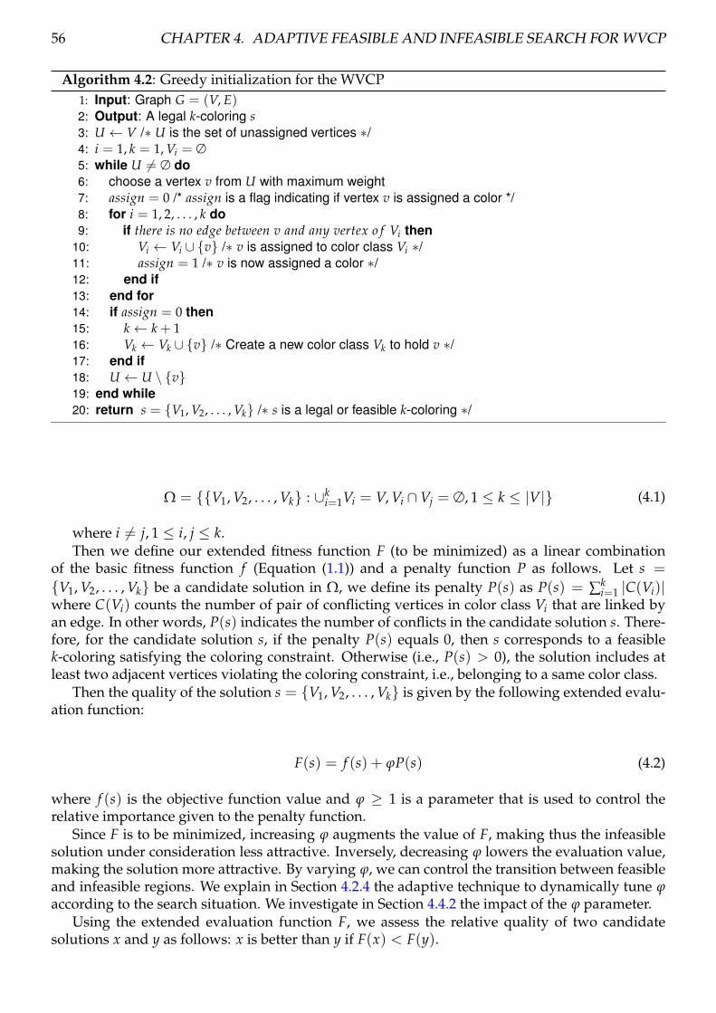
56 CHAPTER 4. ADAPTIVE FEASIBLE AND INFEASIBLE SEARCH FOR WVCP
Algorithm 4.2: Greedy initialization for the WVCP1: Input: Graph G = (V, E)2: Output: A legal k-coloring s3: U ← V /∗ U is the set of unassigned vertices ∗/4: i = 1, k = 1, Vi = ∅5: while U 6= ∅ do6: choose a vertex v from U with maximum weight7: assign = 0 /* assign is a flag indicating if vertex v is assigned a color */8: for i = 1, 2, . . . , k do9: if there is no edge between v and any vertex o f Vi then
10: Vi ← Vi ∪ v /∗ v is assigned to color class Vi ∗/11: assign = 1 /∗ v is now assigned a color ∗/12: end if13: end for14: if assign = 0 then15: k← k + 116: Vk ← Vk ∪ v /∗ Create a new color class Vk to hold v ∗/17: end if18: U ← U \ v19: end while20: return s = V1, V2, . . . , Vk /∗ s is a legal or feasible k-coloring ∗/
Ω = V1, V2, . . . , Vk : ∪ki=1Vi = V, Vi ∩Vj = ∅, 1 ≤ k ≤ |V| (4.1)
where i 6= j, 1 ≤ i, j ≤ k.Then we define our extended fitness function F (to be minimized) as a linear combination
of the basic fitness function f (Equation (1.1)) and a penalty function P as follows. Let s =
V1, V2, . . . , Vk be a candidate solution in Ω, we define its penalty P(s) as P(s) = ∑ki=1 |C(Vi)|
where C(Vi) counts the number of pair of conflicting vertices in color class Vi that are linked byan edge. In other words, P(s) indicates the number of conflicts in the candidate solution s. There-fore, for the candidate solution s, if the penalty P(s) equals 0, then s corresponds to a feasiblek-coloring satisfying the coloring constraint. Otherwise (i.e., P(s) > 0), the solution includes atleast two adjacent vertices violating the coloring constraint, i.e., belonging to a same color class.
Then the quality of the solution s = V1, V2, . . . , Vk is given by the following extended evalu-ation function:
F(s) = f (s) + ϕP(s) (4.2)
where f (s) is the objective function value and ϕ ≥ 1 is a parameter that is used to control therelative importance given to the penalty function.
Since F is to be minimized, increasing ϕ augments the value of F, making thus the infeasiblesolution under consideration less attractive. Inversely, decreasing ϕ lowers the evaluation value,making the solution more attractive. By varying ϕ, we can control the transition between feasibleand infeasible regions. We explain in Section 4.2.4 the adaptive technique to dynamically tune ϕaccording to the search situation. We investigate in Section 4.4.2 the impact of the ϕ parameter.
Using the extended evaluation function F, we assess the relative quality of two candidatesolutions x and y as follows: x is better than y if F(x) < F(y).
4.2. ADAPTIVE FEASIBLE AND INFEASIBLE SEARCH FOR THE WVCP 57
4.2.4 Searching feasible and infeasible solutions with tabu search
Neighborhood and its evaluation
The AFISA algorithm examines the search space Ω by making transitions from the currentsolution to one neighboring solution. A neighboring solution is generated by using the popular“one-move" operator. Give a solution s = V1, V2, . . . , Vk, the one-move operator displaces avertex v from its current color class Vi to a different color class Vj (i 6= j, j ∈ 1, 2, . . . , |V|),leading to a neighboring solution designated by s ⊕ < v, Vi, Vj >. The one-move neighborhoodis then given by:
N(s) = s ⊕ < v, Vi, Vj > : v ∈ Vi, 1 ≤ i ≤ k, 1 ≤ j ≤ |V|, i 6= j (4.3)
This neighborhood allows a vertex to be moved to a currently empty color class Vj with j > k(thus the number of color classes can increase). Inversely, a color class can also become empty andthus be removed when its last vertex is transferred to another existing class (thus k is decreased).As a result, search algorithms using this neighborhood like the tabu search procedure presentedin Section 4.2.4 typically visit solutions whose number of color classes varies during the search.
Notice that this neighborhood is different from the one-move neighborhood used for othercoloring problems (e.g., conventional vertex coloring [Galinier and Hertz, 2006; Malaguti andToth, 2010] and equitable coloring problem [Lai et al., 2015; Sun et al., 2017; Wang et al., 2018],because 1) in these studies the vertex v ∈ Vi to be displaced must be a conflicting vertex (i.e.,there exists in Vi at least another vertex u such that v and u are adjacent in the graph), and 2) thenumber of color classes k remains fixed.
Finally, one important issue concerns the evaluation of the neighborhood that impacts signif-icantly the computational efficiency of any local search algorithm. In our case, we employ anincremental evaluation technique that is similar to the evaluation technique designed for anothergraph coloring problem (i.e., equitable coloring) [Lai et al., 2015; Sun et al., 2017]. With this tech-nique, the objective variation of each neighbor solution can be conveniently obtained in constanttime. We refer the readers to [Lai et al., 2015; Sun et al., 2017] for more details of this evaluationtechnique.
Tabu search
To explore the above neighborhood, the proposed AFISA algorithm uses the well-known tabusearch (TS) meta-heuristic [Glover, 1989; Glover, 1990] that has been applied to many difficultcombinatorial optimization problems [Glover, 1997]. In particular, TS is known to be quite suc-cessful in solving several different graph coloring problems such as general graph coloring [Galin-ier and Hao, 1999; Hertz and de Werra, 1987], minimum sum coloring [Jin and Hao, 2016] andequitable coloring [Lai et al., 2015]. As a general meta-heuristic, TS has some attractive features.First, it can be adapted to graph coloring problems rather easily. Moreover, TS offers simplestrategies to promote a suitable and necessary search balance between intensification (with thebest-improvement principle to explore a given neighbourhood) and diversification (with a tabulist).
In our case, the tabu search procedure make transitions between various k-colorings guidedby the extended evaluation function F of Section 4.2.3. Our TS procedure is based on the popularTabuCol algorithm for the conventional Vertex Coloring Problem [Hertz and de Werra, 1987] andadopts the improvements presented in [Galinier and Hao, 1999]. For the sake of completeness, weshow the pseudo-code of the tabu search procedure in Algorithm 4.3 and provide the followingdescription.

58 CHAPTER 4. ADAPTIVE FEASIBLE AND INFEASIBLE SEARCH FOR WVCP
The tabu search procedure iteratively replaces the current solution s by a neighboring solutions′ taken from the one-move neighborhood N(s) defined in Section 4.2.4 until a stopping conditionis met. At each iteration, TS examines the neighborhood and selects a best admissible neighboringsolution s′ (see below) to substitute s. After each iteration, the associate one-move is recordedon the tabu list to prevent the search from revisiting s for the next tt iterations (tt is called thetabu tenure). To tune the tabu tenure, we use tt = Random(A) + αF where F stands for theextended evaluation function, the function Random(A) returns a random number in 0, . . . ,A-1(A is set to 10 in this work) and α is a parameter set to 0.6. Meanwhile, the best solution found isupdated if the new solution is better than all previous visited solutions. A neighboring solution s′
is considered to be admissible if it is not forbidden by the tabu list or if it is better (according to theextended evaluation function F) than the best solution found. If the best solution is not updatedduring β consecutive iterations (β is called the depth of tabu search), then the current tabu searchprocess is considered to be stagnating and stops.
Algorithm 4.3: Tabu search algorithm1: Input: initial solution s, depth of tabu search β2: Output: The best solution sb found during the tabu search process3: sc ← s /* sc is the current solution */4: sb ← sc /* sb is the best solution found */5: d← 0 /* d counts the consecutive iterations during which sb is not updated */6: repeat7: Choose a best admissible neighboring solution s′ ∈ N(sc)
/* s′ is admissible if it is not forbidden by the tabu list or better than sb */8: sc ← s′
9: /* Update the best solution */10: if F(sc) < F(sb) then11: sb ← sc12: d← 013: else14: d← d + 115: end if16: until d = β17: return sb
Adaptive mechanism to control feasible and infeasible searches
The AFISA algorithm uses the extended evaluation function F (see Section 4.2.3) combiningthe objective function f and the penalty function P to assess the quality of candidate solutionsand guide the search process. By varying the penalty coefficient ϕ of F, we can change the searchtrajectory according to the search situation. Basically, a large (small) ϕ value strongly (weakly)penalizes infeasible solutions and incites the search process to give more importance to feasible(infeasible) solutions. To allow the search process to go back and forth between feasible andinfeasible zones, we devise an adaptive mechanism to dynamically adjust ϕ such that a suitablediversification-intensification balance can be reached. This adaptive mechanism relies on knownideas proposed for continuous optimization like those reviewed in [Hamida and Schoenauer,2000].
The adaptive adjustment mechanism is shown in Algorithm 4.4. According to whether thesolution s (obtained from the last round of tabu search) is a feasible k-coloring, we adjust ϕ toinfluence the search trajectory of the next round of tabu search. Specifically, if P(s) 6= 0 (i.e.,
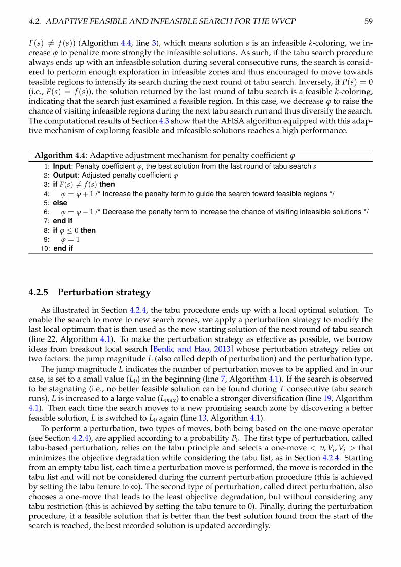
4.2. ADAPTIVE FEASIBLE AND INFEASIBLE SEARCH FOR THE WVCP 59
F(s) 6= f (s)) (Algorithm 4.4, line 3), which means solution s is an infeasible k-coloring, we in-crease ϕ to penalize more strongly the infeasible solutions. As such, if the tabu search procedurealways ends up with an infeasible solution during several consecutive runs, the search is consid-ered to perform enough exploration in infeasible zones and thus encouraged to move towardsfeasible regions to intensify its search during the next round of tabu search. Inversely, if P(s) = 0(i.e., F(s) = f (s)), the solution returned by the last round of tabu search is a feasible k-coloring,indicating that the search just examined a feasible region. In this case, we decrease ϕ to raise thechance of visiting infeasible regions during the next tabu search run and thus diversify the search.The computational results of Section 4.3 show that the AFISA algorithm equipped with this adap-tive mechanism of exploring feasible and infeasible solutions reaches a high performance.
Algorithm 4.4: Adaptive adjustment mechanism for penalty coefficient ϕ
1: Input: Penalty coefficient ϕ, the best solution from the last round of tabu search s2: Output: Adjusted penalty coefficient ϕ3: if F(s) 6= f (s) then4: ϕ = ϕ + 1 /* Increase the penalty term to guide the search toward feasible regions */5: else6: ϕ = ϕ− 1 /* Decrease the penalty term to increase the chance of visiting infeasible solutions */7: end if8: if ϕ ≤ 0 then9: ϕ = 1
10: end if
4.2.5 Perturbation strategy
As illustrated in Section 4.2.4, the tabu procedure ends up with a local optimal solution. Toenable the search to move to new search zones, we apply a perturbation strategy to modify thelast local optimum that is then used as the new starting solution of the next round of tabu search(line 22, Algorithm 4.1). To make the perturbation strategy as effective as possible, we borrowideas from breakout local search [Benlic and Hao, 2013] whose perturbation strategy relies ontwo factors: the jump magnitude L (also called depth of perturbation) and the perturbation type.
The jump magnitude L indicates the number of perturbation moves to be applied and in ourcase, is set to a small value (L0) in the beginning (line 7, Algorithm 4.1). If the search is observedto be stagnating (i.e., no better feasible solution can be found during T consecutive tabu searchruns), L is increased to a large value (Lmax) to enable a stronger diversification (line 19, Algorithm4.1). Then each time the search moves to a new promising search zone by discovering a betterfeasible solution, L is switched to L0 again (line 13, Algorithm 4.1).
To perform a perturbation, two types of moves, both being based on the one-move operator(see Section 4.2.4), are applied according to a probability P0. The first type of perturbation, calledtabu-based perturbation, relies on the tabu principle and selects a one-move < v, Vi, Vj > thatminimizes the objective degradation while considering the tabu list, as in Section 4.2.4. Startingfrom an empty tabu list, each time a perturbation move is performed, the move is recorded in thetabu list and will not be considered during the current perturbation procedure (this is achievedby setting the tabu tenure to ∞). The second type of perturbation, called direct perturbation, alsochooses a one-move that leads to the least objective degradation, but without considering anytabu restriction (this is achieved by setting the tabu tenure to 0). Finally, during the perturbationprocedure, if a feasible solution that is better than the best solution found from the start of thesearch is reached, the best recorded solution is updated accordingly.

60 CHAPTER 4. ADAPTIVE FEASIBLE AND INFEASIBLE SEARCH FOR WVCP
4.2.6 Connections with existing studies
For the WVCP considered in this work, one notices that existing heuristic algorithms [Malagutiet al., 2009; Prais and Ribeiro, 2000] visit only feasible solutions while ignoring infeasible solutions.As such, these algorithms could encounter difficulties when the feasible solutions are scatteredin different zones that are separated by infeasible zones. In this work, we explore for the firsttime the idea of searching both feasible and infeasible solutions for solving the WVCP. Indeed, asillustrated in other settings, e.g., [Chen et al., 2016b; Martinez-Gavara et al., 2017; Sun et al., 2017;Wang et al., 2018], such a mixed search strategy is highly effective for solving several difficultproblems (e.g., capacitated arc routing, capacitated clustering and equitable coloring). Amongthese studies, two of them [Sun et al., 2017; Wang et al., 2018] are worthy of a special mention,because they consider the related equitable coloring problem (ECP). Given that the WVCP stud-ied in this work and the ECP considered in [Sun et al., 2017; Wang et al., 2018] are two differentcoloring problems, our work posses several particular features that distinguish itself from thesestudies.
First, the proposed AFISA algorithm incorporates search components (dedicated neighbor-hood, specific penalty-based evaluation function, perturbation technique...) that are customizedto the WVCP. Second, unlike [Sun et al., 2017; Wang et al., 2018] where different algorithms aredesigned to search separately feasible and infeasible solutions, AFISA uses the same tabu searchprocedure to exploit both types of solutions, making the algorithm simpler in design and imple-mentation. Third, AFISA integrates an adaptive mechanism to dynamically control the feasibleand infeasible searches by the self-tuned parameter ϕ. Such a mechanism is missing in the stud-ies mentioned above. Fourth, unlike [Sun et al., 2017; Wang et al., 2018], AFISA does not solve aseries of k-coloring problems where each coloring problem is defined for a fixed number of colorsk. Instead, the number of colors k varies during the search of our algorithm as explained in Sec-tion 4.2.4. Finally, as we show in Section 4.3, the proposed algorithm integrating these featurescompetes very favorably with the state of the art methods for the WVCP in the literature.
4.3 Experimental results and comparisons
This section is dedicated to a large experimental assessment of the proposed AFISA algorithmfor solving the WCVP and comparisons with other state of the art methods. The study is basedon 111 conventional benchmark instances in the literature as well as 50 new (large) instances fromthe DIMACS and COLOR competitions.
4.3.1 Benchmark instances
Test instances. We consider 111 instances from the literature on the WCVP [Cornaz et al., 2017;Malaguti et al., 2009; Prais and Ribeiro, 2000] and 50 additional instances from the DIMACS andCOLOR competitions initially proposed for the conventional graph coloring problems 1, 2. Weclassify these instances into four sets.
1. The first set contains 46 (small) instances from the DIMCAS/COLOR competitions. Graphsof this set have DSJC∗, GEOM∗ or R∗ in their name with up to 125 vertices. The exactalgorithm (MWSS) [Cornaz et al., 2017] is able to find the optimal solutions for 40 instancesin this set. These instances are tested in [Cornaz et al., 2017; Malaguti et al., 2009], whoseresults will be used as our references.
1. http://www.dimacs.rutgers.edu/2. http://www.cs.hbg.psu.edu/txn131/graphcoloring.html

4.3. EXPERIMENTAL RESULTS AND COMPARISONS 61
2. The second set contains 35 instances from matrix-decomposition problems. These graphsnamed as pxx have up to 138 vertices and 1186 edges. The exact algorithm (MWSS) [Cornazet al., 2017] is able to find the optimal solutions for all graphs in this set. These instances aretested in [Cornaz et al., 2017; Malaguti et al., 2009; Prais and Ribeiro, 2000], whose resultswill be used as our references.
3. The third set contains 30 rxx instances proposed in [Prais and Ribeiro, 2000] from matrix-decomposition problems. These instances have the same structure as the pxx instances, butare larger, having up to 301 vertices and 4122 edges. These instances are tested in [Cornazet al., 2017; Prais and Ribeiro, 2000] and the exact algorithm (MWSS) [Cornaz et al., 2017] isable to find the optimal solutions for all graphs in this set.
4. The fourth set contains 50 additional larger instances (with at least 120 vertices) 3. These in-stances are created by adding random vertex weights between 1 to 20 to DIMACS/COLORgraphs.
4.3.2 Experimental settings
The proposed algorithm was coded in C++ and compiled by GNU g++ 4.1.2 with -O3 flag(option). The experiments were conducted on a computer with an Intel Xeon E5-2670 processor(2.5 GHz and 2 GB RAM) running Ubuntu 12.04. When solving the DIMACS machine benchmarkprocedure ‘dfmax.c’ 4 without compilation optimization flag, the run time on the computer is 0.46,2.68 and 10.70 seconds for graphs r300.5, r400.5 and r500.5, respectively.
Parameters. The setting of the parameters is given in Table 4.1, which was determined by apreliminary experiment. For this, we first identify a rough range of values for each parameter. Toidentify the default value of a particular parameter, we test different values from the range whilefixing the other parameters to their default values (typically those of Table 4.1). As to the penaltycoefficient ϕ of the extended evaluation function F, it is tuned adaptively as explained in Section4.2.4. We use the default setting of Table 4.1 to report the experimental results shown in the restof this chapter, though fine-tuning some parameters could lead to improved results.
Table 4.1 – Settings of important parameters
Parameters Description Value
L0 , Lmax Small and large jump magnitude 0.05*N, 0.5*NT Max number of non-improving local optima visited before strong perturb 50P0 Probability for applying tabu-based or direct perturbation 0.7β Depth of tabu search 100,N < 50
10000, N > 50
Reference algorithms. For our comparative study, we use the most recent heuristic algorithms[Malaguti et al., 2009; Prais and Ribeiro, 2000] as our references. The GRASP algorithm [Praisand Ribeiro, 2000] was run on an IBM 9672 model R34 mainframe computer under a limit of1000 iterations. The 2_Phase algorithm [Malaguti et al., 2009] was run on a PIV 2.4 MHz with512 MB RAM under Windows XP and tested by stopping phase 1 after 500 iterations and phase2 after 75 seconds. When solving the DIMACS machine benchmark procedure ‘dfmax.c’, therun time on the instance r500.5 reported in [Malaguti et al., 2009] for this machine is 7 seconds(against 10.7 seconds for our computer). We also include the lower and upper bounds reportedby the exact algorithm MWSS in [Cornaz et al., 2017]. The results of MWSS were obtained ona computer equipped with an Intel Xeon E3-1220 at 3.10 GHz with 8 GB RAM, which spent 4.5
3. These new instances are available at:http://www.info.univ-angers.fr/~hao/wvcp.html
4. dfmax:ftp://dimacs.rutgers.edu/pub/dsj/clique/

62 CHAPTER 4. ADAPTIVE FEASIBLE AND INFEASIBLE SEARCH FOR WVCP
seconds to solve the benchmark instance r500.5 (this computer is roughly 2 times faster than ourcomputer). These bounds provide useful information when they are contrasted with the results(upper bounds) obtained by the compared heuristic algorithms (GRASP, 2_Phase and AFISA).
Following [Barr et al., 1995], we show computational results in terms of solution quality andcomputation time. Since computation time can be greatly biased by many factors like comput-ing platform, programming language, data structures and so on, solution quality is the primarycriterion while timing information is provided only for indicative purposes.
Stopping condition. Following [Malaguti et al., 2009; Prais and Ribeiro, 2000], we ran ourAFISA algorithm 20 times for the instances from the first, second and fourth sets with a cutofftime of 1 hour per run. For the rxx instances of the third set, a cutoff time of 4 hours is used in[Cornaz et al., 2017] used on their computer (Intel Xeon E3-1220 processor, 3.10 GHz and 8 GBRAM), which roughly corresponds to 8 hours on our computer. We set a cutoff time of 2 hoursfor the instances with up to 200 vertices and 4 hours for larger instances for our AFISA algorithm(longer times do not lead to significantly improved results). Finally, note that for 8 instances ofthe first set that cannot be solved by MWSS [Cornaz et al., 2017] in 1 hour, a large time limit of10 hours was allowed (marked with ~ in Table 4.2), leading to optimality proof of two instances(R100_1g and R100_1gb).
4.3.3 Computational results and comparisons with state-of-the-art algorithms
Table 4.2 – Comparative results of AFISA with state-of-the-art algorithms on the 46 DIMACSbenchmark instances. Improved upper bounds are indicated in bold.
Instance |V| |E| BKVAFISA MWSS 2_Phase
∆1 ∆2Best SR Avg t(s) Best t(s) Best t(s)DSJC125_1g.col~ 125 736 24 23 2 24.0 3016.32 25 36000.0 24 152 -2 -1DSJC125_1gb.col~ 125 736 95 90 1 92.5 402.57 95 36000.0 95 170 -5 -5DSJC125_5g.col~ 125 3891 76 71 2 72.3 216.04 78 36000.0 76 180 -7 -5DSJC125_5gb.col~ 125 3891 251 243 1 250.2 369.34 263 36000.0 251 182 -20 -8DSJC125_9g.col 125 6961 169∗ 169∗ 3 169.9 16.00 169∗ 0.3 169∗ 162 0 0DSJC125_9gb.col 125 6961 604∗ 604∗ 3 605.5 443.96 604∗ 0.4 605 237 0 -1GEOM100.col 100 547 65∗ 65∗ 20 65.0 0.81 65∗ 3.8 65∗ 131 0 0GEOM100a.col 100 992 89∗ 89∗ 10 89.5 110.42 89∗ 2.4 89∗ 112 0 0GEOM100b.col 100 1050 32∗ 32∗ 1 33.1 59.11 32∗ 3.8 32∗ 15 0 0GEOM110.col 110 638 68∗ 68∗ 20 68.0 33.81 68∗ 59.5 69 172 0 -1GEOM110a.col 110 1207 97∗ 97∗ 6 97.8 176.76 97∗ 12.9 97∗ 111 0 0GEOM110b.col 110 1256 37∗ 37∗ 14 37.9 130.85 37∗ 5.0 37∗ 5 0 0GEOM120.col 120 773 72∗ 72∗ 20 72.0 33.14 72∗ 157 72∗ 157 0 0GEOM120a.col 120 1434 105∗ 105∗ 1 106.3 156.00 105∗ 7.0 105∗ 136 0 0GEOM120b.col 120 1491 35∗ 35∗ 7 37.3 67.72 35∗ 16.5 35∗ 14 0 0GEOM30b.col 30 81 12∗ 12∗ 20 12.0 0.02 12∗ 0.0 12∗ 0 0 0GEOM40b.col 40 157 16∗ 16∗ 20 16.0 0.03 16∗ 0.1 16∗ 1 0 0GEOM50b.col 50 249 18∗ 18∗ 20 18.0 0.02 18∗ 0.1 18∗ 0 0 0GEOM60b.col 60 366 23∗ 23∗ 20 23.0 0.22 23∗ 0.5 23∗ 0 0 0GEOM70.col 70 267 47∗ 47∗ 20 47.0 4.99 47∗ 0.3 47∗ 96 0 0GEOM70a.col 70 459 73∗ 73∗ 20 73.0 4.42 73∗ 0.4 73∗ 3 0 0GEOM70b.col 70 488 24∗ 24∗ 20 24.0 12.03 24∗ 0.9 24∗ 6 0 0GEOM80.col 80 349 66∗ 66∗ 20 66.0 2.11 66∗ 1.1 66∗ 0 0 0GEOM80a.col 80 612 76∗ 76∗ 19 76.1 137.1 76∗ 1.1 76∗ 102 0 0GEOM80b.col 80 663 27∗ 27∗ 5 27.8 66.8 27∗ 2.5 27∗ 90 0 0GEOM90.col 90 441 61∗ 61∗ 16 61.2 88.92 61∗ 2.0 61∗ 166 0 0GEOM90a.col 90 789 73∗ 73∗ 3 74.0 512.41 73∗ 4.8 73∗ 157 0 0GEOM90b.col 90 860 30∗ 30∗ 19 30.1 67.38 30∗ 1.7 30∗ 11 0 0R100_1g.col~ 100 509 21∗ 21∗ 1 22.0 113.77 21∗ 28788.5 22 155 0 -1R100_1gb.col~ 100 509 81∗ 81∗ 1 83.8 3.04 81∗ 9362.2 - 171 0 -R100_5g.col~ 100 2456 59 59 5 60.1 6.97 59 36000.0 - 179 0 -R100_5gb.col~ 100 2456 225 221 1 224.1 186.81 225 36000.0 - 179 -4 -R100_9g.col 100 4438 141∗ 141∗ 15 141.3 21.36 141∗ 0.1 - 123 0 -R100_9gb.col 100 4438 518∗ 518∗ 1 549.3 1152.83 518∗ 0.3 - 127 0 -R50_1g.col 50 108 14∗ 14∗ 20 14.0 0.14 14∗ 0.8 14∗ 0 0 0R50_1gb.col 50 108 53∗ 53∗ 20 53.0 0.24 53∗ 1.6 53∗ 95 0 0R50_5g.col 50 612 37∗ 37∗ 20 37.0 0.95 37∗ 1.4 37∗ 167 0 0R50_5gb.col 50 612 135∗ 135∗ 14 135.3 3.72 135∗ 1.5 137 145 0 -2R50_9g.col 50 1092 74∗ 74∗ 20 74.0 0.74 74∗ 0.0 74∗ 36 0 0R50_9gb.col 50 1092 262∗ 262∗ 20 262.0 12.61 262∗ 0.0 262∗ 33 0 0R75_1g.col 70 251 18∗ 18∗ 12 18.4 10.96 18∗ 132.8 19 154 0 -1R75_1gb.col 70 251 70∗ 70∗ 19 70.1 2.46 70∗ 192.2 72 166 0 -2R75_5g.col 75 1407 51∗ 51∗ 12 51.4 0.08 51∗ 1056.0 53 172 0 -2R75_5gb.col 75 1407 186∗ 186∗ 2 189.0 19.42 186∗ 989.3 190 173 0 -4R75_9g.col 75 2513 110∗ 110∗ 20 110.0 2.65 110∗ 0.0 110∗ 79 0 0R75_9gb.col 75 2513 396∗ 396∗ 12 396.4 145.89 396∗ 0.0 399 50 0 -3#Better 5/46 0/46 0/41#Equal 41/46 43/46 32/41#Worse 0/46 3/46 9/41p_value - 2.5e-2 3.1e-4
Table 4.2 reports the results of our AFISA algorithm on the first set of 46 DIMACS/COLOR

4.3. EXPERIMENTAL RESULTS AND COMPARISONS 63
instances commonly used in the literature, together with the results of the reference algorithmsMWSS [Cornaz et al., 2017] and 2_Phase [Malaguti et al., 2009]. The first 3 columns indicate foreach instance its name, the number of vertices and the number of edges. The fourth column showsthe best-known value (BKV) reported in the literature [Cornaz et al., 2017; Malaguti et al., 2009;Prais and Ribeiro, 2000]. The next four columns show the results of the AFISA algorithm foreach instance: the best result (i.e., the smallest objective function value) over 20 independent runs(Best), the success rate (SR) to achieve the best result over 20 runs, the average result (Avg) andthe average computation time (in seconds) of the successful runs to obtain the best result (t(s)) (0is given if the time is less than 0.009 second). The following four columns report the results andthe computation time obtained by the reference algorithms (MWSS and 2_Phase). For MWSS, theindicated time corresponds to the time of 1000 iterations. For 2_Phase, the time is the sum of thetime of 500 iterations of phase 1 and the time of phase 2. The last two columns (∆1,∆2) indicate thedifference between our result (Best) and the result of MWSS and 2_Phase. To verify the statisticalsignificance of the comparisons between AFISA and each reference algorithm, we show in the row"p-values" the results from the non-parametric Friedman test applied to the best values of AFISAand each compared algorithm, and a p-value smaller than 0.05 implies a significant differencebetween two compared results.
Additionally, the rows #Better, #Equal and #Worse indicate respectively the number of in-stances for which an algorithm performs better, equally well or worse compared to the best-known values (BKV).
Finally, an entry with ∗ indicates the optimal objective value. A bold entry highlights an im-proved upper bound, i.e., an improved result over the current best-known value. Entries with "-"mean that the corresponding results are not available in the literature.
Table 4.3 – Comparative results of AFISA with state-of-the-art algorithms on the 35 pxx bench-mark instances. Improved upper bounds are indicated in bold.
Instance |V| |E| BKVAFISA MWSS 2_Phase GRASP
∆1 ∆2 ∆3Best SR Avg t(s) Best t(s) Best t(s) Best t(s)p06.col 16 38 565∗ 565∗ 20 565.0 0 565∗ 0.0 565∗ 0.4 565∗ 1.1 0 0 0p07.col 24 92 3771∗ 3771∗ 20 3771.0 0.02 3771∗ 0.0 3771∗ 0.1 3771∗ 4.0 0 0 0p08.col 24 92 4049∗ 4049∗ 20 4049.0 0.17 4049∗ 0.0 4049∗ 1.3 4049∗ 1.3 0 0 0p09.col 25 100 3388∗ 3388∗ 16 3388.2 0.95 3388∗ 0.0 3388∗ 0.1 3388∗ 3.0 0 0 0p10.col 16 32 3983∗ 3983∗ 20 3983.0 0.68 3983∗ 0.0 3983∗ 0.1 3983∗ 4.5 0 0 0p11.col 18 48 3380∗ 3380∗ 20 3380.0 0.01 3380∗ 0.0 3380∗ 0.1 3380∗ 4.7 0 0 0p12.col 26 90 657∗ 657∗ 20 657.0 0 657∗ 0.0 657∗ 0.1 657∗ 3.8 0 0 0p13.col 34 160 3220∗ 3220∗ 17 3221.1 0.68 3220∗ 0.0 3225 2.3 3230 7.8 0 -5 -10p14.col 31 110 3157∗ 3157∗ 20 3157.0 0 3157∗ 0.0 3157∗ 0.1 3157∗ 10.1 0 0 0p15.col 34 136 341∗ 341∗ 20 341.0 1.81 341∗ 0.0 341∗ 0.1 341∗ 4.7 0 0 0p16.col 34 134 2343∗ 2343∗ 20 2343.0 0.76 2343∗ 0.0 2343∗ 0.5 2343∗ 14.5 0 0 0p17.col 37 161 3281∗ 3281∗ 7 3322.2 2.72 3281∗ 0.0 3281∗ 1.4 3281∗ 5.5 0 0 0p18.col 35 143 3228∗ 3228∗ 20 3228.0 0.05 3228∗ 0.0 3228∗ 0.2 3228∗ 10.4 0 0 0p19.col 36 156 3710∗ 3710∗ 20 3710.0 0.36 3710∗ 0.0 3710∗ 0.1 3710∗ 14.6 0 0 0p20.col 37 142 1830∗ 1830∗ 13 1841.0 4.86 1830∗ 0.0 1830∗ 1.3 1860 20.0 0 0 -30p21.col 38 155 3660∗ 3660∗ 19 3660.5 0.75 3660∗ 0.0 3660∗ 0.2 3660∗ 18.4 0 0 0p22.col 38 154 1912∗ 1912∗ 18 1912.2 0.29 1912∗ 0.0 1912∗ 0.2 1912∗ 20.0 0 0 0p23.col 44 204 3770∗ 3770∗ 3 3793.0 0.28 3770∗ 0.1 3770∗ 1.4 3810 21.4 0 0 -40p24.col 34 104 661∗ 661∗ 20 661.0 0 661∗ 0.0 661∗ 0.1 661∗ 27.9 0 0 0p25.col 36 120 504∗ 504∗ 20 504.0 0.28 504∗ 0.0 504∗ 0.1 504∗ 23.9 0 0 0p26.col 37 131 520∗ 520∗ 20 520.0 0.11 520∗ 0.0 520∗ 0.1 520∗ 28.3 0 0 0p27.col 44 174 216∗ 216∗ 20 216.0 0.08 216∗ 0.1 216∗ 0.2 216∗ 7.8 0 0 0p28.col 44 174 1729∗ 1729∗ 14 1735.1 2.56 1729∗ 0.1 1729∗ 0.1 1729∗ 44.5 0 0 0p29.col 53 254 3470∗ 3470∗ 20 3470.0 0.10 3470∗ 0.1 3470∗ 65.7 3470∗ 65.7 0 0 0p30.col 60 317 4891∗ 4891∗ 20 4891.0 53.79 4891∗ 0.2 4891∗ 2.1 4891∗ 56.6 0 0 0p31.col 47 179 620∗ 620∗ 20 620.0 3.69 620∗ 0.1 620∗ 0.1 620∗ 70.9 0 0 0p32.col 51 221 2480∗ 2480∗ 20 2480.0 0.35 2480∗ 0.1 2480∗ 0.0 2480∗ 70.9 0 0 0p33.col 56 258 3018∗ 3018∗ 7 3029.7 0.43 3018∗ 0.3 3018∗ 0.1 3018∗ 62.3 0 0 0p34.col 74 421 1980∗ 1980∗ 19 1980.5 3.05 1980∗ 0.6 1980∗ 0.1 1980∗ 131.9 0 0 0p35.col 86 566 2140∗ 2140∗ 15 2145.0 4.48 2140∗ 0.6 2140∗ 0.1 2140∗ 135.0 0 0 0p36.col 101 798 7210∗ 7210∗ 12 7385.0 0.13 7210∗ 1.4 7210∗ 0.1 7210∗ 163.1 0 0 0p38.col 87 537 2130∗ 2130∗ 1 2139.5 9.54 2130∗ 1.2 2130∗ 0.4 2130∗ 231.8 0 0 0p40.col 86 497 4984∗ 4984∗ 1 5016.6 5.05 4984∗ 1.0 4984∗ 0.2 4984∗ 224.2 0 0 0p41.col 116 900 2688∗ 2688∗ 2 2688.1 0.10 2688∗ 3.2 2688∗ 0.1 2688∗ 313.7 0 0 0p42.col 138 1186 2466∗ 2466∗ 4 2671.2 930.96 2466∗ 3.2 2509 2.8 2480 405.8 0 -43 -14#Better 0/35 0/35 0/35 0/35#Equal 35/35 35/35 33/35 31/35#Worse 0/35 0/35 2/35 4/35p-value - - 1.6e-1 4.6e-2
From Table 4.2, we observe that AFISA reaches a remarkable performance on the first set of46 DIMACS/COLOR instances. Compared to the most recent exact algorithm MWSS, AFISAattains all known optimal results (40 cases). For 5 out of the 6 remaining instances whose optimal

64 CHAPTER 4. ADAPTIVE FEASIBLE AND INFEASIBLE SEARCH FOR WVCP
Table 4.4 – Comparative results of AFISA with state-of-the-art algorithms on the 30 rxx bench-mark instances. Improved upper bounds are indicated in bold.
Instance |V| |E| BKVAFISA MWSS GRASP
∆1 ∆2Best SR Avg t(s) Best t(s) Best t(s)r01.col 144 1280 6724∗ 6724∗ 8 6727.8 49.57 6724∗ 17.6 6724∗ 887 0 0r02.col 142 1246 6771∗ 6771∗ 3 6780.6 85.33 6771∗ 11.3 6771∗ 1041 0 0r03.col 139 1188 6473∗ 6473∗ 10 6490.8 190.19 6473∗ 10.4 6475 966 0 -2r04.col 151 1406 6342∗ 6342∗ 1 6403.2 467.37 6342∗ 11.4 6342∗ 989 0 0r05.col 142 1266 6408∗ 6408∗ 1 6466.3 71.68 6408∗ 12.3 6409 904 0 -1r06.col 148 1381 7550∗ 7550∗ 4 7555.9 29.24 7550∗ 10.3 7550∗ 899 0 0r07.col 141 1253 6889∗ 6889∗ 3 7555.9 34.76 6889∗ 13.7 6889∗ 6889 0 0r08.col 138 1191 6057∗ 6057∗ 1 6080.3 311.66 6057∗ 4.1 6076 810 0 -19r09.col 129 1027 6358∗ 6358∗ 1 6393.8 395.24 6358∗ 9.5 6424 868 0 -66r10.col 150 1409 6508∗ 6508∗ 1 6519.3 461.98 6508∗ 13.1 6525 1048 0 -17r11.col 208 2247 7654∗ 7654∗ 1 7710.6 259.25 7654∗ 57.2 7669 2423 0 -15r12.col 199 2055 7690∗ 7691 1 7710.4 9542.18 7690∗ 53.7 7691 2267 1 0r13.col 217 2449 7500∗ 7521 1 7558.3 619.53 7500∗ 105.2 7524 2365 21 -3r14.col 214 2387 8254∗ 8254∗ 1 8283.9 8044.07 8254∗ 65.3 8254∗ 2342 0 0r15.col 198 2055 8021∗ 8021∗ 1 8126.8 2559.06 8021∗ 25.1 8021∗ 2395 0 0r16.col 188 1861 7755∗ 7755∗ 2 7789.2 195.53 7755∗ 26.7 7755∗ 2696 0 0r17.col 213 2392 7979∗ 7979∗ 2 8030.3 855.38 7979∗ 79.3 8025 3175 0 -46r18.col 200 2079 7232∗ 7232∗ 1 7278.9 868.19 7232∗ 58.2 7232∗ 1902 0 0r19.col 185 1803 6826∗ 6840 1 6868.1 395.5 6826∗ 32.7 6858 2082 14 -18r20.col 217 2447 8023∗ 8023∗ 1 8102.0 1028.5 8023∗ 104.1 8027 3452 0 -4r21.col 281 3554 9284∗ 9284∗ 1 9384.5 4588.72 9284∗ 390.0 9287 4948 0 -3r22.col 285 3684 8887∗ 8887∗ 1 8959.3 12911 8887∗ 302.6 8887∗ 5603 0 0r23.col 288 3732 9136∗ 9136∗ 1 9267.9 3251.96 9136∗ 375.3 9145 5887 0 -9r24.col 269 3284 8464∗ 8464∗ 1 8572.9 13142.6 8464∗ 201.7 8464∗ 4997 0 0r25.col 266 3177 8426∗ 8468 1 8560.8 874.75 8426∗ 225.6 8504 5139 42 -36r26.col 284 3629 8819∗ 8819∗ 1 8927.9 14225.1 8819∗ 439.6 8819∗ 5462 0 0r27.col 259 3019 7975∗ 7975∗ 1 8019.7 14074.9 7975∗ 248.1 7975∗ 5064 0 0r28.col 288 3765 9407∗ 9407∗ 1 9599.4 8691.00 9407∗ 222.7 9407∗ 5874 0 0r29.col 281 3553 8693∗ 8693∗ 1 8743.7 7613.14 8693∗ 388.0 8693∗ 4923 0 0r30.col 301 4122 9816∗ 9816∗ 1 10003.2 8838.59 9816∗ 346.9 9816∗ 6145 0 0#Better 0/30 0/30 0/30#Equal 26/30 30/30 16/30#Worse 4/30 0/30 14/30p-value - 4.6e-2 3.2e-4
Table 4.5 – Comparative results of FISA with CPLEX on the additional set of 50 larger DI-MACS/COLOR instances. Improved upper bounds are indicated in bold.
Instance |V| |E|AFISA CPLEX
∆Best SR Avg t(s) UB LB statusmiles250.col 128 387 102∗ 8 102.7 56.61 102∗ 102∗ Optimal 0miles500.col 128 1170 260 1 261.3 48.46 - - - -miles1000.col 128 3216 432 1 444.7 480.02 437 31.692 Feasible -5miles1500.col 128 5198 587 1 644.3 32.31 - - - -mulsol.i.5.col 186 3973 367.0 20 367.0 416.91 360 109.034 Feasible 7queen10_10.col 100 2940 166 3 169.2 68.43 - - - -queen11_11.col 121 3960 178 1 182.3 55.24 - - - -queen12_12.col 144 5192 194 1 198.6 92.7 208 47.000 Feasible -14queen13_13.col 169 6656 204 2 207.5 199.85 - - - -queen14_14.col 196 8372 224 2 227.4 360.05 316 23.000 Feasible -92queen15_15.col 225 10360 237 1 241.2 183.44 - - - -queen16_16.col 256 12640 253 2 256.3 300.85 365 22.033 Feasible -112zeroin.i.1.col 211 4100 518 20 518.0 0 - - - -zeroin.i.2.col 211 3541 336 3 337.6 440.84 300 26.103 Feasible 36zeroin.i.3.col 206 3540 299 2 301.7 139.64 - - - -DSJC250.1.col 250 3218 140 1 141.9 48.94 - - - -DSJC250.5.col 250 15668 415 1 428.1 269.23 - - - -DSJC250.9.col 250 55794 925 1 942.7 856.25 - - - -DSJC500.1.col 500 12458 210 1 215.6 426.64 - - - -DSJC500.5.col 500 125248 778 1 845.1 159.27 - - - -DSJC500.9.col 500 224874 1790 1 1854.5 831.07 - - - -DSJR500.1.col 500 3555 169 1 175.4 458.86 - - - -DSJC1000.1.col 1000 99258 359 4 362.9 430.54 - - - -DSJC1000.5.col 1000 499652 1357 1 1430.9 371.65 - - - -DSJC1000.9.col 1000 898898 3166 1 3231.0 490.2 - - - -inithx.i.1.col 864 18707 587 5 587.9 527.46 - - - -inithx.i.2.col 645 13979 341 8 341.6 0.03 - - - -inithx.i.3.col 621 13969 352 11 355.6 0.01 - - - -le450_15a.col 450 8168 241 1 247.1 288.37 - - - -le450_15b.col 450 8169 239 2 245.1 368.35 - - - -le450_15c.col 450 16680 313 1 320.8 432.95 - - - -le450_15d.col 450 16750 306 2 314.1 113.7 - - - -le450_25a.col 450 8260 317 1 329.9 362.26 - - - -le450_25b.col 450 8263 318 1 325.8 285.88 - - - -le450_25c.col 450 17343 378 1 387.9 359.37 - - - -le450_25d.col 450 17345 375 1 385.3 254.76 - - - -flat1000_50_0.col 1000 245000 1289 1 1315.7 981.77 - - - -flat1000_60_0.col 1000 245830 1338 1 1354 201.98 - - - -flat1000_76_0.col 1000 246708 1314 1 1337.6 2396.63 - - - -C2000.5.col 2000 999836 2400 1 2425.1 3133.97 - - - -C2000.9.col 2000 1799532 6228 1 6284.0 2798.3 - - - -latin_square_10.col 900 307350 1690 1 1900.0 780.26 - - - -wap01a.col 2368 110871 638 1 653.1 1133.51 - - - -wap02a.col 2464 111742 637 1 638.1 3270.46 - - - -wap03a.col 4730 286722 687 1 707.5 2901.51 - - - -wap04a.col 5231 294902 698 1 709.0 4.79 - - - -wap05a.col 905 43081 598 1 610.9 1574.52 - - - -wap06a.col 947 43571 599 1 607.6 65.32 - - - -wap07a.col 1809 103368 680 1 692.5 384.82 - - - -wap08a.col 1870 104176 663 1 673.4 2627.2 - - - -#Better 47/50 2/7#Equal 1/50 1/7#Worse 2/50 4/7

4.4. ANALYSIS 65
values are still unknown, AFISA improves the current best upper bounds (see negative entriesin column ∆1). AFISA also dominates the 2_Phase algorithm on the 41 instances tested by bothalgorithms, by obtaining better results for 13 instances (see negative entries in column ∆2) and thesame results for the remaining 28 instances. The small p-values (< 0.05) indicates that there is asignificant difference between our best results and those of the two reference algorithms MWSS(p-value=2.5e-2) and 2_Phase (p-value=3.1e-4).
Table 4.3 reports the comparative results on the first set of 35 pxx instances from matrix-decomposition problems with one more reference algorithm (GRASP) [Prais and Ribeiro, 2000].One observes that AFISA performs very well on these pxx instances. AFISA attains always theknown optimal values of MWSS, while 2_Phase and GRASP miss 2 and 4 instances respectively.The difference between AFISA and 2_Phase is however not statistically significant (p-value of1.6e-1), while the difference between AFISA and GRASP is significant with a p-value of 4.6e-2.
Table 4.4 shows the results of AFISA on the second set of 30 rxx instances from matrix-decomposition problems, along with those of MWSS and GRASP. Table 4.4 indicates that AFISAfinds the optimal solutions for 26 out of the 30 rxx instances, which were previously obtainedby the exact algorithm MWSS. Among the four cases where AFISA misses the optimal solution,the gap to the optimal value is no more than 0.498% (instance r25). Compared to the referenceheuristic algorithm GRASP, AFISA (Column 4) dominates GRASP by attaining 13 better and 17equal results. The p-value of 4.6e-2 between AFISA and MWSS indicates that there is a slightdifference and the p-value of 3.2e-4 between AFISA and GRASP indicates that there is significantdifference between the results of AFISA and GRASP.
Notice that according to [Malaguti et al., 2009], 2_Phase is able to find (in comparable com-puting times) 3 solutions better than those of GRASP reported in [Prais and Ribeiro, 2000], 9solutions of equal quality and 18 worse solutions. However the detailed results of 2_Phase on therxx instances are not available.
Finally, Table 4.5 summarizes our results on the set of 50 additional (larger) DIMACS/COLORinstances. Since these instances are not tested previously by any WVCP method, we use thegeneral MIP solver CPLEX (version 12.6) as our reference method. We run CPLEX, with a cutofflimit of one hour, to solve the 0/1 ILP model shown in Appendix 5.6. Entries with − in Table 4.5indicate that no feasible solution is found by CPLEX within the time limit and this happens for43 out of the 50 instances. The last column (∆) indicates the difference between our best resultand the upper bound of CPLEX (a negative value implies thus a better result). We observe thatonly one instance can be solved to optimality by CPLEX within the one hour time limit. For thesix instances for which CPLEX reaches a feasible solution, but fails to find the optimal solution,its upper bounds are worse than the bounds of AFISA in four cases. Due to the small number ofinstances solved by CPLEX, we omit the statistical test.
To sum up, this computational assessment indicates that AFISA performs very well on thefour sets of benchmark instances. The new upper bounds (5 for the first set and the results for thefourth set) established by AFISA can serve as valuable reference values to evaluate future algo-rithms for the WVCP. Meanwhile, AFISA failed to attain the optimal values for four instances ofthe third set, indicating there is room for further improvement. Finally, this experimental studyconfirms that like for many NP-hard problems, both exact and heuristic algorithms are comple-mentary and can be used to solve problem instances of different sizes and different characteristics.These approaches can even be combined to create powerful hybrid algorithms.
4.4 Analysis
This section performs additional experiments to analyze the benefits of three important in-gredients of the proposed AFISA algorithm: the penalty coefficient of the extended evaluation

66 CHAPTER 4. ADAPTIVE FEASIBLE AND INFEASIBLE SEARCH FOR WVCP
1 2 3 4
250
255
260
265
(a) DSJC125_5gb.col
1 2 3 4
2500
2600
2700
2800
(b) p42.col
1 2 3 4
6900
7000
7100
7200
(c) r05.col
1 2 3 4
255
260
265
(d) queen16_16.col
Figure 4.1 – Influence of the increment/decrement value of the penalty efficient
function, the strategy of visiting both feasible and infeasible solutions and the perturbation strat-egy.
4.4.1 Impact of the penalty coefficient
AFISA uses the extended evaluation function F defined in Section 4.2.3 to explore both feasi-ble and infeasible solutions. The oscillation between feasible and infeasible zones is adaptivelycontrolled by increasing or decreasing the penalty coefficient ϕ (≥ 1). In this study, we analyzethe impact of the increment/decrement value used to adjust ϕ and for this purpose, we test thefollowing increment/decrement values: 1,2,3,4 (larger values make the search oscillate too muchbetween feasible and infeasible zones).
Box and whisker plots of the results on 4 representative instances from the four benchmark sets(which are relatively difficult according to Tables 4.2-4.5) are shown in Figure 4.1, where the X-axisindicates the tested increment/decrement values and the Y-axis indicates the objective values. Asa supplement, we also compute the p-value for each tested instance. The results are based on 20

4.4. ANALYSIS 67
independent runs for each instance with a cutoff time of 300 seconds per run. One observes thatthe performance of the AFISA algorithm is significantly influenced by the increment/decrementvalue on the instances DSJC125_5gb (p-value = 1.4e-2) and queen16_16 (p-value = 1.2e-4). This isless the case for the instances p42 (p-value = 2.0e-1) and r05 (p-value = 7.6e-1). Furthermore, theAFISA algorithm with the increment/decrement value of 1 gives the best performance comparedto other values. This explains why we adopt 1 as the default increment/decrement value in thisstudy. Finally, one notices that the outcome of this experiment remains coherent with the intuitiveunderstanding that the search will go back and forth more frequently between feasible and infea-sible regions with a large increment/decrement value than with a small value. This implies that alarge increment/decrement value may make the search leave each newly discovered (feasible orinfeasible) zone too early before the search zone is sufficiently exploited.
4.4.2 Benefit of searching both feasible and infeasible solutions
Table 4.6 – Assessment of searching both feasible and infeasible solutions. The better results arein bold.
Instance |V| |E|AFISA Tabu_Feasible
∆Best SR Avg t(s) Best SR Avg t(s)
DSJC1000.1.col 1000 99258 359 4 362.9 430.54 354 1 358.9 450.15 5DSJC1000.5.col 1000 499652 1357 1 1430.9 371.65 1354 1 1371.3 84.75 3DSJC1000.9.col 1000 898898 3166 1 3231.0 490.2 3166 1 3231.1 490.2 0DSJC125_1g.col 125 736 23 2 24.0 3016.32 23 4 23.8 1467.63 0DSJC125_1gb.col 125 736 90 1 92.5 402.57 91 1 94.6 30.09 -1DSJC125_5g.col 125 3891 71 2 72.3 216.04 71 1 72.5 199.14 0DSJC125_5gb.col 125 3891 243 1 250.2 369.34 246 3 250.9 292.08 -3DSJC125_9g.col 125 6961 169 3 170.0 16 169 4 170.2 42.1 0DSJC125_9gb.col 125 6961 604 3 605.0 443.96 606 2 608.7 18.24 -2DSJC250.1.col 250 3218 140 1 141.9 48.94 140 4 142.1 57.37 0DSJC250.5.col 250 15668 415 1 428.1 269.23 421 1 431.2 318.86 -6DSJC250.9.col 250 55794 925 1 942.7 856.25 948 1 965.8 365.4 -23DSJC500.1.col 500 12458 210 1 215.6 426.64 212 1 215.3 84.83 -2DSJC500.5.col 500 125248 778 1 845.1 159.27 780 1 796.1 450.89 -2DSJC500.9.col 500 224874 1790 1 1854.5 831.07 1791 1 1869.2 345.13 -1DSJR500.1.col 500 3555 169 1 175.4 458.86 170 2 171.9 272.89 -1GEOM100.col 100 547 65 20 65.0 0.81 65 20 65.0 9.86 0miles1500.col 128 5198 587 1 644.3 32.31 797 4 798.6 0.13 -210p13.col 34 160 3220 17 3221.1 0.68 3220 16 3221.5 0.83 0p20.col 37 142 1830 13 1841 4.86 1830 16 1835.5 0.76 0p42.col 138 1186 2466 4 2671.2 930.96 2646 1 2659.7 12.51 -180queen12_12.col 144 5192 194 1 198.6 92.7 196 2 199.0 96.04 -2queen14_14.col 196 8372 224 2 227.4 360.05 225 1 227.7 129.47 -1queen16_16.col 256 12640 253 2 256.3 300.85 250 1 254.8 14.15 3r03.col 139 1188 6473 10 6490.8 190.19 6487 1 6536 119.3 -14r05.col 142 1266 6408 1 6466.3 71.68 6495 1 6525.6 143.13 -87R100_1g.col 100 509 21 1 22.0 113.77 21 3 21.9 533.65 0R100_5g.col 100 2456 59 5 60.1 6.97 59 2 60.3 2.56 0R100_5gb.col 100 2456 221 1 224.1 186.81 222 1 224.7 1362.52 -1R100_9g.col 100 4438 141 15 141.3 21.36 141 11 141.5 2.43 0R100_9gb.col 100 4438 518 1 549.3 1152.83 518 13 518.5 21.25 0R50_5gb.col 50 612 135 14 135.3 3.72 135 18 135.3 0.11 0R75_1g.col 70 251 18 12 18.4 10.96 18 10 18.5 32.89 0R75_1gb.col 70 251 70 19 70.1 2.46 70 17 70.3 6.58 0R75_5g.col 75 1407 51 12 51.4 0.08 51 7 51.7 5.11 0R75_5gb.col 75 1407 186 2 189.0 19.42 186 2 189.2 31.93 0R75_9gb.col 75 2513 396 12 396.4 145.89 396 9 396.7 4.35 0zeroin.i.2.col 211 3541 336 3 337.6 440.84 336 13 336.4 0.91 0#Better 16/38 24/38 3/38 12/38#Equal 19/38 2/38 19/38 2/38#Worse 3/38 12/38 16/38 24/38p_value - - 2.9e-3 4.6e-2
To assess the strategy of oscillating between feasible and infeasible regions of the proposedalgorithm, we create a algorithmic variant (called Tabu_Feasible) in which the search visits onlyfeasible solutions. For this, we set the penalty coefficient ϕ of the extended evaluation function(Eq. (4.2), Section 4.2.3) to a large value in order to penalize strongly any infeasible solution. Inour case, ϕ is set to the largest weight of vertices of the given graph. For this experiment, weselect 38 instances that are relatively difficult according to the results reported in Tables 4.2-4.5,i.e., their best-known results cannot consistently be attained by all algorithms. We ran 20 timesboth algorithms to solve each selected instance with a cutoff time of 1 hour.
The comparative results of this experiment are presented in Table 4.6 with the same informa-tion as before. The rows #Better/#Equal/#Worse indicate the number of instances for which each

68 CHAPTER 4. ADAPTIVE FEASIBLE AND INFEASIBLE SEARCH FOR WVCP
algorithm attain a better, equal and worse result compared to the other algorithm in terms of thebest objective value found. The last column indicates the difference between the best results ofAFISA and Tabu_Feasible. We observe that even if both algorithms obtain 19 equal results, AFISAachieves 16 better results (against 3 for Tabu_Feasible). The small p-values (< 0.05) in terms ofBest and Avg confirm the statistical significance of the reported differences between AFISA andTabu_Feasible. This experiment shows that searching both feasible and infeasible solutions en-ables the algorithm to reach a better performance.
4.4.3 Impact of the perturbation operation
Table 4.7 – Assessment of the perturbation strategy. The better results are in bold.
Instance |V| |E|AFISA AFISA−
∆Best SR Avg t(s) Best SR Avg t(s)
DSJC1000.1.col 1000 99258 359 4 362.9 430.54 384 10 385.5 0.08 -25DSJC1000.5.col 1000 499652 1357 1 1430.9 371.65 1427 10 1434.5 0.07 -70DSJC1000.9.col 1000 898898 3166 1 3231.0 490.2 3291 10 3302.5 0.04 -125DSJC125_1g.col 125 736 23 2 24.0 3016.32 33 6 33.7 0 -10DSJC125_1gb.col 125 736 90 1 92.5 402.57 120 13 122.8 0 -30DSJC125_5g.col 125 3891 71 2 72.3 216.04 87 14 88.5 0 -16DSJC125_5gb.col 125 3891 243 1 250.2 369.34 293 20 293.0 0.01 -50DSJC125_9g.col 125 6961 169 3 170.0 16 186 12 188.8 0 -17DSJC125_9gb.col 125 6961 604 3 605.0 443.96 652 10 668.0 0 -48DSJC250.1.col 250 3218 140 1 141.9 48.94 168 10 170.5 0.01 -28DSJC250.5.col 250 15668 415 1 428.1 269.23 472 8 476.5 0 -57DSJC250.9.col 250 55794 925 1 942.7 856.25 1039 11 1060.0 0 -114DSJC500.1.col 500 12458 210 1 215.6 426.64 242 10 243.0 0.02 -32DSJC500.5.col 500 125248 778 1 845.1 159.27 853 8 856.0 0.03 -75DSJC500.9.col 500 224874 1790 1 1854.5 831.07 1937 20 1937.0 0.01 -147DSJR500.1.col 500 3555 169 1 175.4 458.86 184 10 191.5 0.01 -15GEOM100.col 100 547 65 20 65.0 0.81 74 9 74.6 0.01 -9miles1500.col 128 5198 587 1 644.3 32.31 799 8 809.8 0 -212p13.col 34 160 3220 17 3221.1 0.68 3568 7 3764.3 0 -348p20.col 37 142 1830 13 1841.0 4.86 2270 20 2270 0.01 -440p42.col 138 1186 2466 4 2671.2 930.96 2880 12 2887.2 0 -414queen12_12.col 144 5192 194 1 198.6 92.7 229 9 230.0 0 -35queen14_14.col 196 8372 224 2 227.4 360.05 254 14 255.5 0 -30queen16_16.col 256 12640 253 2 256.3 300.85 280 9 282.2 0 -27r03.col 139 1188 6473 10 6490.8 190.19 6603 1 6687.3 376.19 -130r05.col 142 1266 6408 1 6466.3 71.68 6495 2 6637.7 0 -87R100_1g.col 100 509 21 1 22.0 113.77 30 8 30.6 0 -9R100_5g.col 100 2456 59 5 60.1 6.97 72 10 73.5 0 -13R100_5gb.col 100 2456 221 1 224.1 186.81 260 1 264 0 -39R100_9g.col 100 4438 141 15 141.3 21.36 153 9 157.4 0 -12R100_9gb.col 100 4438 518 1 549.3 1152.83 548 9 551.5 0 -30R50_5gb.col 50 612 135 14 135.3 3.72 152 8 156.8 0 -17R75_1g.col 70 251 18 12 18.4 10.96 24 7 25.2 0 -6R75_1gb.col 70 251 70 19 70.1 2.46 88 11 89.4 0 -18R75_5g.col 75 1407 51 12 51.4 0.08 63 20 63.0 0 -12R75_5gb.col 75 1407 186 2 189.0 19.42 231 11 233.7 0 -45R75_9gb.col 75 2513 396 12 396.4 145.89 425 12 428.2 0.01 -29zeroin.i.2.col 211 3541 336 3 337.6 440.84 337 13 337.7 0 -1#Better 38/38 38/38 0/38 0/38#Equal 0/38 0/38 0/38 0/38#Worse 0/38 0/38 38/38 38/38p-value - - 7.1e-10 7.1e-10
As shown in Section 4.2.5, the proposed algorithm uses a perturbation strategy as an addi-tional means of diversification. To assess this strategy, we compare AFISA with a AFISA variant(denoted as AFISA−) where the perturbation strategy is disabled (i.e., by removing line 22 in Al-gorithm 4.1). This experiment is based on the 38 instances used in Section 4.4.2. We ran 20 timesboth algorithms to solve each selected instance with a cutoff time of 1 hour.
The results of this experiment are shown in Table 4.7 with the same statistics as before. Weobserve that AFISA dominates, in terms of Best and Avg, the AFISA− variant by obtaining abetter result for each instance. The small p-values confirm the dominance of AFISA over AFISA−.This experiment demonstrates the interest of the adopted perturbation strategy as a meaningfulmeans of diversification that enables the algorithm to better explore the search space.

4.5. CONCLUSIONS 69
4.5 Conclusions
The weighted vertex coloring problem (WVCP) considered in this work is a generalizationof the conventional vertex coloring problem with a number of practical applications. Motivatedby the observation that existing methods limit their search to feasible solutions, we investigatedfor the first time the benefit of examining both feasible and infeasible solutions for solving theproblem. The resulting AFISA algorithm oscillates between feasible and infeasible search zonesguided by an extended evaluation function that combines the initial objective function and anadaptive penalty function. To explore feasible and infeasible spaces, we introduced a tabu searchprocedure enhanced by a dedicated perturbation strategy to escape local optima traps.
We assessed the performance of the AFISA algorithm on three sets of 111 instances commonlytested in the literature and an additional set of 50 (large) DIMACS and COLOR instances ini-tially proposed for graph coloring problems. We presented 5 improved best results (new upperbounds) among the 111 instances of the literature and the first upper bounds for the new set of 50instances. These new bounds can serve as valuable references to assess future WVCP algorithmsand might be used by a branch-and-bound algorithm as high-quality initial bounds. This studydemonstrates the benefit of the search strategy examining both feasible and infeasible solutionsfor solving the WVCP. The computational results on different types of benchmark instances alsoconfirm that exact and heuristic algorithms are complementary solution approaches that can beadvantageously employed to handle instances of different sizes with particular features.
For future work, several directions could be followed. First, other penalty-based evaluationfunctions could be devised to enable a better strategic oscillation between feasible and infeasiblespaces. Second, other neighborhoods (rather than the one-move based neighborhood used inthis work) can be sought to further improve the performance of the search algorithm. Third, theproposed algorithm could be advantageously integrated into a hybrid population-based method(e.g., memetic search, path-linking) as a key intensification component. Fourth, this work usestabu search to explore candidate solutions. Other meta-heuristics can be investigated to ensurethis task while reusing most algorithmic components of AFISA. Finally, few exact algorithmsare available for the WVCP, there is thus much room for research in this direction. In this context,AFISA could be used to generate high-quality initial bounds or to obtain upper bound estimationsof subproblems during the search process.


5Iterated backtrack removal search for findingk-VCS
In this chapter, we propose an iterated backtrack-based removal (IBR) heuristic to find k-VCSfor a given graph. IBR extends the popular removal strategy with two new search components– a backtracking mechanism to reconsider some removed vertices and a perturbation strategy toescape local optima traps. Computational results on 80 benchmark graphs show that IBR is verycompetitive in terms of solution quality and run-time efficiency compared with state-of-the-artalgorithms in the literature. Specifically, IBR improves best-known solutions for 9 graphs andmatches the best results for other 70 instances. An article describing IBR is published in Journalof Heuristics [Sun et al., 2018a].
Contents5.1 Introduction . . . . . . . . . . . . . . . . . . . . . . . . . . . . . . . . . . . . . . . . . 725.2 Notations . . . . . . . . . . . . . . . . . . . . . . . . . . . . . . . . . . . . . . . . . . 725.3 The Iterated Backtrack-based Removal Algorithm . . . . . . . . . . . . . . . . . . 73
5.3.1 General structure of the IBR algorithm . . . . . . . . . . . . . . . . . . . . . . 735.3.2 The removal algorithm . . . . . . . . . . . . . . . . . . . . . . . . . . . . . . . 765.3.3 Heuristic coloring algorithm . . . . . . . . . . . . . . . . . . . . . . . . . . . 765.3.4 Backtrack-based removal approach . . . . . . . . . . . . . . . . . . . . . . . 775.3.5 Perturbation operator of backtrack-based removal algorithm . . . . . . . . . 785.3.6 Update procedure . . . . . . . . . . . . . . . . . . . . . . . . . . . . . . . . . 79
5.4 Experimental results and analysis . . . . . . . . . . . . . . . . . . . . . . . . . . . . 815.4.1 Experiment settings . . . . . . . . . . . . . . . . . . . . . . . . . . . . . . . . 815.4.2 Instances and experimental settings . . . . . . . . . . . . . . . . . . . . . . . 835.4.3 Comparison with state of the art algorithm . . . . . . . . . . . . . . . . . . . 83
5.5 Analysis and discussions . . . . . . . . . . . . . . . . . . . . . . . . . . . . . . . . . 855.5.1 Effectiveness of different backtrack strategies for k-VCS detection . . . . . . 865.5.2 Effectiveness of perturbation for k-VCS detection . . . . . . . . . . . . . . . 865.5.3 Effectiveness of backtrack for k-VCS detection . . . . . . . . . . . . . . . . . 87
5.6 Conclusion . . . . . . . . . . . . . . . . . . . . . . . . . . . . . . . . . . . . . . . . . 87
71

72 CHAPTER 5. ITERATED BACKTRACK REMOVAL SEARCH FOR FINDING K-VCS
5.1 Introduction
This chapter is dedicated to the k-vertex-critical subgraphs problem which was introduced inChapter 1. Recall that given an undirected graph G = (V, E) and a positive integer k, a k-vertex-critical subgraph (k-VCS) of G is a subgraph H such that its chromatic number equals k (i.e.,χ(H) = k), and removing any vertex causes a decrease of χ(H). The k-VCS problem (k-VCSP) isto find the smallest k-vertex-critical subgraph H∗ of G. We extend previous studies by proposingan Iterated Backtrack Removal Search (IBR) for finding k-VCS in a graph. IBR reinforces theclassical removal procedure [Chinneck, 1997b; Chinneck and Dravnieks, 1991; Desrosiers et al.,2008; Herrmann and Hertz, 2002] with a backtracking scheme and a perturbation strategy. Thebasic idea of our approach is as follows. The removal procedure reduces the current graph bytentatively moving vertices to the set of uncritical vertices (see Section 5.3.2). This process isrepeated until the subgraph induced by set of critical vertices is such that its chromatic numberequals k. If the current subgraph does contain a k-VCS (the chromatic number of the currentsubgraph less than k), which means some critical vertices were removed to the set of uncriticalvertices in error, the backtracking procedure is invoked. The backtracking procedure expands thecurrent subgraph by adding back some vertices which are in the set of the uncritical vertices untilthe chromatic number of the current subgraph increases to k again. The perturbation procedureprovides a means of reconsidering some vertices which would have been incorrectly identified ascritical ones (see Section 5.3.5). This phase terminates once the stop condition is met.
We assess the proposed IBR algorithm on 80 popular DIMACS and COLOR02-04 benchmarkinstances which are commonly used to test k-VCS algorithms in the literature . The experimentalresults show that our IBR algorithm competes favorably with the state-of-the-art results. Specif-ically, the proposed algorithm improves best-known solutions for 9 graphs (improves the lowerbound for 6 instances, at the same k, IBR obtains a better solution (smaller size of k-VCS) for 8instances) and matches the best results for other 70 instances. Only in one case, IBR obtains aslightly worse result.
The chapter is organized as follows. Section 5.2 introduces some useful notations. Section5.3 presents the components of the IBR algorithm, including the basic removal algorithm, thebacktrack-based removal algorithm and the perturbation procedure. Section 5.4 shows computa-tional evaluation and comparisons with state-of-the-art results. Section 5.5 investigates the keycomponents of the proposed algorithm, followed by conclusions in Section 5.6.
5.2 Notations
Let G = (V, E) be an input graph, we introduce the following notations, which are useful forthe description of the proposed approach.
We define three working sets of vertices A, B and C that are used by the algorithm. For eachvertex of V, we first define its status (critical, unknown, uncritical).
A critical vertex is a vertex that belongs to a k-VCS. We use A to denote the set of critical verticesthat have been detected. A is also called the critical set.
An unknown or undetected vertex is a vertex whose status is still unknown. We use B to denotethe set of unknown vertices, which is also called the unknown set.
An uncritical vertices refers to a vertex that does not belong to a k-VCS. We use C to denote theset of uncritical vertices, which is also called the uncritical set.
Given the critical set A and the unknown set B, the subgraph induced by A, H = GA =(A, EA) (EA = A× A ∩ E), is called the critical subgraph of G. The subgraph induced by A ∪ B,GA∪B = (A ∪ B, EA∪B) (EA∪B = ((A ∪ B)× (A ∪ B)) ∩ E), is the remaining subgraph of G.
As explained in the next section, the proposed approach operates on these three sets of ver-

5.3. THE ITERATED BACKTRACK-BASED REMOVAL ALGORITHM 73
tices, which are initially set as A = ∅, B = V, C = ∅. Then the algorithm searches a k-VCSby moving vertices from one set to another according to the temporarily identified status of eachvertex.
For any vertex i, we also associate a weight w(i), which is defined as follows:
w(i) =
|E|, i f i ∈ A.1, i f i ∈ B;0, i f i ∈ C;
(5.1)
At the beginning of the search, we set w(i) = 1 for each vertex i of V (since A = ∅, B = V, C =∅). The weight of a vertex is updated each time the vertex changes its status (critical, unknown,uncritical) (see Section 5.3). The weight information is mainly used by the removal algorithm forvertex selection.
5.3 The Iterated Backtrack-based Removal Algorithm
In this section, we present the iterated backtrack-based removal algorithm (IBR) for detectingk-VCS in a graph. IBR extends the classical removal algorithm with a backtracking scheme and aperturbation procedure.
5.3.1 General structure of the IBR algorithm
Given a graph G = (V, E) and an integer k ≤ K (K being χ(G) or the smallest number of colorsfor which a k-coloring exists), the proposed IBR algorithm (see Figure 5.1 and Algorithm 5.1) aimsto find a small k-VCS, i.e., a small set of critical vertices A ⊆ V such that the induced subgraphH = (A, EA) has a chromatic number of χ(H) = k, and removing any vertex from H decreasesχ(H).
The IBR algorithm operates with three working sets of vertices, initialized as A = ∅, B =V, C = ∅. Basically, according to the coloring results on the remaining graph provided by aheuristic coloring algorithm, IBR uses three main procedures to move vertices among these setsin order to find a k-VCS.
Recall that each graph G contains at least one k-VCS for 1 ≤ k ≤ χ(G). Furthermore, a graphG is (k− 1)-colorable if and only if G does not contain a k-VCS. Note that the problem of decidingwhether a graph G is (k − 1)-colorable is itself NP-hard. For this reason, we adopt a heuristiccoloring algorithm Color (see Section 5.3.3) to judge whether G is (k− 1)-colorable.
1. The removal procedure inspects, one by one, the vertices of set B of unknown vertices to de-termine their status (Algorithm 5.1, lines 7-16). Specifically, at each iteration, a vertex i fromB is first moved to C (i.e., i is supposed to be uncritical, line 8). If the graph GA∪B afterremoving i does not contains a k-VCS any longer, i.e., becomes (k− 1)-colorable, (checkedwith a heuristic coloring algorithm, see Section 5.3.3), then vertex i is identified as criticaland moved from C to A (lines 9-10, see Section 5.3.2). We check again with the heuristic col-oring algorithm whether the graph GA∪B contains a k-VCS (line 12). If the graph GA∪B afteradding i back still does not contain a k-VCS, then certain critical vertices were incorrectlyclassified into the uncritical set C, a backtracking procedure is invoked (line 12). This processis repeated until the subgraph induced by set A of critical vertices is such that its chromaticnumber equals k (line 7).
2. Since the algorithm used to judge whether the remaining graphs GA∪B contains a k-VCS isnot an exact algorithm (see Section 5.3.3), a critical vertex can be incorrectly classified into

74 CHAPTER 5. ITERATED BACKTRACK REMOVAL SEARCH FOR FINDING K-VCS
Algorithm 5.1: The IBR algorithm for solving the k-VCSP1: Input: Graph G = (V, E), integer k ≤ K (K being χ(G) or the smallest number of colors for which a
k-coloring exists), R maximum allowed perturbations.2: Output: H the smallest k-colorable subgraph
/*Initialization*/3: H1 = ∅, · · · , HR = ∅ /* each Hr records a detected candidate k-VCS*/4: A = ∅, B = V, C = ∅, H = (A, EA) /*A is set of critical vertices, B is set of unknown vertices, C is set
of uncritical vertices*/5: r = 0 /*r is the number of performed perturbations*/6: while r < R do7: while H does not contains a k-VCS do8: Choose a vertex i ∈ B, move i from B to C /*vertex removal, Section 5.3.2*/9: if GA∪B does not contains a k-VCS then
10: move i from C to A /*i is detected as a critical vertex*/11: H = (A, EA)
/*Backtracking, Section 5.3.4*/12: while GA∪B does not contains a k-VCS do13: Choose a vertex l ∈ C, move l from C to B14: end while15: end if16: end while17: r = r + 118: Hr = H
/*Perturbation operator for the critical subgraph*/19: H′ ← Perturbation(Hr) /*Section 5.3.5*/
/*Update the set A, B and C*/20: A, B, C ← Update_set(H′) /*Section 5.3.6*/21: H = (A, EA)22: end while23: H ← the smallest k-colorable subgraph
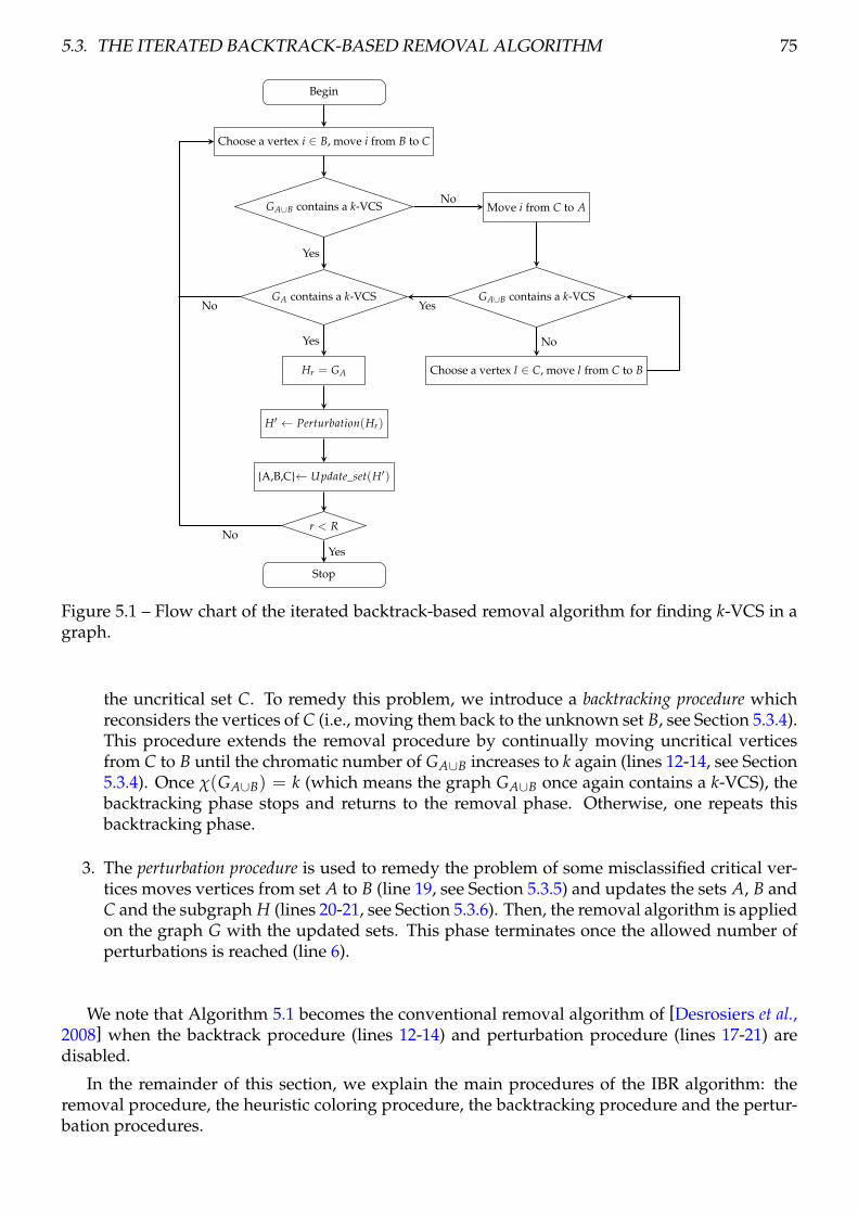
5.3. THE ITERATED BACKTRACK-BASED REMOVAL ALGORITHM 75
Begin
Choose a vertex i ∈ B, move i from B to C
GA∪B contains a k-VCS Move i from C to A
GA contains a k-VCS GA∪B contains a k-VCS
Choose a vertex l ∈ C, move l from C to BHr = GA
H′ ← Perturbation(Hr)
A,B,C← Update_set(H′)
r < R
Stop
No
Yes
Yes
No
Yes
No
YesNo
Figure 5.1 – Flow chart of the iterated backtrack-based removal algorithm for finding k-VCS in agraph.
the uncritical set C. To remedy this problem, we introduce a backtracking procedure whichreconsiders the vertices of C (i.e., moving them back to the unknown set B, see Section 5.3.4).This procedure extends the removal procedure by continually moving uncritical verticesfrom C to B until the chromatic number of GA∪B increases to k again (lines 12-14, see Section5.3.4). Once χ(GA∪B) = k (which means the graph GA∪B once again contains a k-VCS), thebacktracking phase stops and returns to the removal phase. Otherwise, one repeats thisbacktracking phase.
3. The perturbation procedure is used to remedy the problem of some misclassified critical ver-tices moves vertices from set A to B (line 19, see Section 5.3.5) and updates the sets A, B andC and the subgraph H (lines 20-21, see Section 5.3.6). Then, the removal algorithm is appliedon the graph G with the updated sets. This phase terminates once the allowed number ofperturbations is reached (line 6).
We note that Algorithm 5.1 becomes the conventional removal algorithm of [Desrosiers et al.,2008] when the backtrack procedure (lines 12-14) and perturbation procedure (lines 17-21) aredisabled.
In the remainder of this section, we explain the main procedures of the IBR algorithm: theremoval procedure, the heuristic coloring procedure, the backtracking procedure and the pertur-bation procedures.

76 CHAPTER 5. ITERATED BACKTRACK REMOVAL SEARCH FOR FINDING K-VCS
5.3.2 The removal algorithm
Our removal procedure is based on the removal heuristic algorithm presented in [Desrosierset al., 2008], which can be conveniently described using the notion of critical, unknown and un-critical sets of vertices.
After initialization, B = V, A = ∅, C = ∅, H = (A, EA). We note that GA∪B = G is not(k− 1)-colorable, thus contains a k-VCS (see Section 5.3.1 and Algorithm 5.1). In each iteration,the removal algorithm tentatively moves one vertex i from the unknown set B to the uncriticalset C. If GA∪B without vertex i is always not (k− 1)-colorable (i.e., GA∪B contains a k-VCS), theremoved vertex i is considered as an uncritical vertex and is kept in C. Otherwise, if GA∪B withoutvertex i becomes (k− 1)-coloring (i.e., GA∪B does not contain a k-VCS), vertex i is considered as acritical vertex and thus transferred from set C to set A. In both cases, we update the sets A, B, C,the graphs H, GA∪B and the weights of vertices accordingly. The removal algorithm repeats thisprocess until χ(H) increases to k, which occurs when a k-VCS is detected.
In the removal algorithm, the rule used to select the next vertex from B impacts the criticalsubgraphs generated. In order to favor small critical subgraphs, the removal algorithm adoptsthe neighborhood weight heuristic strategy proposed in [Desrosiers et al., 2008], which uses infor-mation contained in the weights of vertices.
Recall that when a vertex i is placed in the set A, B and C, its weight is set as |E|, 1 and 0correspondingly. The neighborhood weight W(i) of a vertex i is defined as the sum of the weightsof the vertices that are adjacent to this vertex. When all weights of vertices are equal to 1 (e.g.,after initialization), the neighborhood weight of a vertex equals its degree and can be consideredas an indicator on the density of the region surrounding this vertex. The neighborhood weightheuristic strategy moves the vertices with the smallest neighborhood weight firstly, and preservesthe denser ones. This strategy proved to be effective to detect a k-VCS with a small size [Desrosierset al., 2008].
5.3.3 Heuristic coloring algorithm
We adopt a heuristic coloring algorithm Color to judge whether a graph G is (k− 1)-colorable(i.e., whether G contains a k-VCS). The removal algorithm can guarantee that the extracted sub-graph H = (A, EA) is a k-VCS when the coloring algorithm Color is an exact algorithm (i.e., ableto verify that the given remaining graph is colorable with a given k). However, given that the gen-eral k-coloring problem is itself NP-complete, exact methods can be too time consuming even forgraphs of relatively small sizes (with several tens of vertices). For this reason and like [Desrosierset al., 2008], we adopt a heuristic coloring algorithm (i.e., TabuCol [Hertz and de Werra, 1987;Dorne and Hao, 1999; Galinier and Hao, 1999]). Contrary to an exact algorithm, the heuristicalgorithm may fail to find a legal coloring with a given k, even if such a coloring exists.
Recall that at each iteration of the removal procedure, we move one unknown vertices i fromB to C. Then, one needs to know whether there is a legal (k− 1)-coloring on graph H = (A, EA)(the stopping condition is met or not) and on graph GA∪B = (A∪ B, EA∪B) (the last moved vertexis critical or not).
To solve the (k − 1)-coloring problem, TabuCol iteratively explores partitions of V in k − 1classes. Each partition c is attributed to a fitness value f (c) which is equal to the number ofedges of the graph that have both endpoints in the class. Therefore, if f (c) = 0, the partition ccorresponds to a proper (k − 1)-coloring. The purpose of the tabu search coloring algorithm isthen to minimize the fitness function f . The tabu coloring process stops when f (c) = 0 or thefitness function cannot be improved within a given number of iterations.

5.3. THE ITERATED BACKTRACK-BASED REMOVAL ALGORITHM 77
Removal
--Unknown vertex
--Critical vertex
--Uncritical vertex
A CBACB
Removal
8
1
12
4
10
5
7
6
11
3
9
2
8
1
12
4
10
5
7
6
11
3
9
2
1
3
5
7
9
11
2
4
6
8
10
12
1
5
7
4
6
3
9
11
2
8
10
12
Figure 5.2 – Removal procedure.
5.3.4 Backtrack-based removal approach
The purpose of the backtracking phase is to cope with the problem caused by the heuristic col-oring algorithm, that some critical vertices may be mistakenly moved to C. This situation happensas follows. When a critical vertex i is moved from B to C, Color should find a legal (k− 1)-coloringin GA∪B with fA∪B = 0 (Algorithm 5.1, line 9), and the vertex i should be moved from C to A (Al-gorithm 5.1, line 10). However, since our coloring algorithm is not an exact method, it may fail tofind a (k− 1)-coloring in GA∪B. In this circumstance, the critical vertex is unexpectedly classifiedto set C and χ(GA∪B) decreases to k − 1. To alleviate this problem, we calls for a backtrackingscheme. When we find a legal (k− 1)-coloring for graph GA∪B, we invoke the backtrack proce-dure, i.e., we move vertices from C to set B, until χ(GA∪B) increases to k again. The key issueconcerns the way to select vertices of C that are moved back to the unknown set B.
To make the choice, we consider two strategies: (1) according to the reverse order by which thevertices have been moved from the set B to the set C; (2) according to the non-increasing order ofneighborhood weights (see Section 5.3.2). Experiments indicated that the first strategy performsquite well and is thus used in this chapter (see Section 5.5.3 for a computational analysis). This canbe explained by the removal heuristic algorithm which prefers vertices with a small neighborhoodweight. Thus, the last moved vertex (with a larger sum of neighborhood weights) has more chanceto be a critical vertex compared to a vertex that was moved since long time. While in rare cases,there are also erroneous movements such that some uncritical vertices are moved to the criticalset A.
To illustrate the procedure, we consider the graph G of Figure 1.4(a) (χ(G) = 4) and a 4-VCSshown in Figure 1.4(b) (with vertices 1, 2, 3, 4, 5, 6, 7). Figure 5.2 shows a possible situation in

78 CHAPTER 5. ITERATED BACKTRACK REMOVAL SEARCH FOR FINDING K-VCS
Backtrack
--Unknown vertex
--Critical vertex
--Uncritical vertex
CBA
Backtrack
8
1
12
4
10
5
7
6
11
3
9
2
8
1
12
4
10
5
7
6
11
3
9
2
1
5
7
4
6
9
8
12
CBA
1
5
7
4
6
3
9
11
2
8
10
12
3
11
2
10
Figure 5.3 – Backtrack-based removal procedure.
the removal procedure: suppose that the coloring algorithm Color fails to find a legal 3-coloringfor GA∪B when the vertices 2, 3 were moved to the uncritical set C, then the vertices 2, 3 are re-tained in the set C. In this case, A = 1, 4, 5, 6, 7, B = ∅, C = 2, 3, 8, 9, 10, 11, 12. Suppose thatafter adding back the last removed vertex 6 to the graph GA∪B, we detected that GA∪B becomes3-colorable (GA∪B does not contain a 4-VCS) using the heuristic coloring algorithm, the backtrack-ing phase is invoked. This involves moving vertices from set C to set A according to the reverse or-der by which the vertices have been moved from set B to set C, until χ(GA∪B) increases to 4 again(GA∪B contains a 4-VCS again). Figure 5.3 illustrates this backtracking procedure for the givengraph G. However, if the uncritical vertex 11 is moved before the last critical vertex was moved,the uncritical vertex 11 will also be moved into the critical set A. Thus A = 1, 2, 3, 4, 5, 6, 7, 11,B = ∅, C = 8, 9, 10, 12. We note that this backtracking procedure is effective for repairing themisjudgments that misclassify critical vertices as uncritical vertices. Meanwhile, this proceduremay unfortunately classify uncritical vertices into the critical set A.
5.3.5 Perturbation operator of backtrack-based removal algorithm
As illustrated in Section 5.3, the backtrack-based removal procedure ends up with a k-VCS(Algorithm 5.1, lines 6-16). However, it may happens that some uncritical vertices are misclas-sified as critical vertices (always due to the use of a heuristic coloring algorithm). To overcomethis problem, we introduce a perturbation procedure, which partially reconfigures A, B and Cby moving some vertices from set A to set B. This procedure also provides new opportunities offinding k-VCS of smaller sizes.
The perturbation procedure (Algorithm 5.2) is inspired by the techniques proposed by [Lü andHao, 2009; Glover et al., 2010], which is decomposed into two parts:

5.3. THE ITERATED BACKTRACK-BASED REMOVAL ALGORITHM 79
Algorithm 5.2: Perturbation1: Input: a k-critical-vertex-subgraph H, a probability threshold p2: Output: a perturbed solution H′ /*Score the vertices in the set A*/3: for i ∈ A do4: calculate score(i) with Equation 5.25: end for6: A
′← η vertices with the highest scores7: A
′← sort A′in descending order of the scores /*Choose and move the perturbed vertices*/
8: for i ∈ A′do
9: i is the jth element in A′, calculate the possibility Pj using Equation 5.3
10: if Pj > p then11: move i from A to B12: end if13: end for14: H′ = (A, EA)
(1) Scoring the vertices in set A. We define a function score(i) to score each vertex i. LetFlipFreq(i) be the number of times vertex i has been displaced among sets A, B and C, EliteSol =[H1, · · · , HR] a set of R critical subgraphs discovered so far (R is the size of EliteSol), EliteFreq(i)the total number of times vertex i appears in EliteSol, the scoring function is then defined as:
sorce(i) = EliteFreq(i)(r− EliteFreq(i))/r2 + (1− FliteFreq(i)/Max_Freq) (5.2)
where 1 ≤ r ≤ R and Max_Freq = maxi∈1...,|V|FlipFreq(i).(2) Choosing and moving the perturbed vertices. We sort all vertices in non-increasing or-
der according to their scores and then choose probabilistically certain vertices from set A. Thepossibility of the jth highly-scored vertex being selected is given by:
Pj =j−1
∑ηz=1 z−1
(5.3)
where η is usually set as |A|/2. Then we move the chosen vertices from set A to set B andupdate the sets A, B and C (see Section 5.3).
As an example, we consider the graph in Figure 5.4 with a chromatic number of 4 and one4-VCS, i.e., 1, 2, 3, 4, 5, 6, 7. Following Section 5.3.4, after the backtrack-based removal proce-dure, A = 1, 2, 3, 4, 5, 6, 7, 11 as critical vertices and other ones are uncritical vertices (C =8, 9, 10, 12, B = ∅), while the vertex 11 is mistaken for a critical vertex. The perturbationprocedure moves certain vertices from set A to set B according to Algorithm 5.2. Figure 5.4(a)and Figure 5.4(b) respectively present two situations where uncritical vertex 2 and the uncriticalvertex 11 are moved from the set A to the set B by the perturbation procedure.
5.3.6 Update procedure
Before invoking a next round of the backtrack-based removal procedure after the perturbationoperation, an additional update operation is applied (Algorithm 5.3). According to whether theperturbed solution contains a k-VCS, we use different strategies to update sets A, B and C. If thesubgraph H′ = (A, EA) does not contain a k-VCS (see Algorithm 5.3, line 4), which means certaincritical vertices are misclassified in set B or even in set C, we move all vertices of C to B in orderto re-examine each vertex of B ∪ C in the next step. Otherwise, we come to the conclusion that

80 CHAPTER 5. ITERATED BACKTRACK REMOVAL SEARCH FOR FINDING K-VCS
Perturbation
--Unknown vertex
--Critical vertex
--Uncritical vertex
CBA
Perturbation
8
1
12
4
10
5
7
6
11
3
9
2
8
1
12
4
10
5
7
6
11
3
9
2
1
6
11
5
7
9
8
12
4
23
10
CBA
1
5
7
4
6
9
8
12
3
11
2
10
(a) Case 1 for the perturbation procedure.
Perturbation
--Unknown vertex
--Critical vertex
--Uncritical vertex
CBA
Perturbation
8
1
12
4
10
5
7
6
11
3
9
2
8
1
12
4
10
5
7
6
11
3
9
2
1
5
7
4
6
9
8
12
3
112
10
CBA
1
5
7
4
6
9
8
12
3
11
2
10
(b) Case 2 for the perturbation procedure.
Figure 5.4 – Perturbation procedure.

5.4. EXPERIMENTAL RESULTS AND ANALYSIS 81
Algorithm 5.3: Update_Set1: Input: a perturbed graph H′ ;2: Output: a update set A, B, C3: fH′ = Color(H′, k− 1)4: if fH′ = 0 then5: move all vertices from C to B /*in order to re-detect each vertex of (B ∪ C) is uncritical or not*/6: else7: move all vertices from B to C /*all the vertices in set B are uncritical vertices*/8: move all vertices from A to B /*in order to rejudge each vertex of A is critical or not*/9: end if
all vertices in set B are uncritical and move all vertices from B to C. Then, in order to determinewhether the vertices of set A are uncritical or not, we move all vertices of A to B.
Following Figure 5.4, after the backtracking procedure and the perturbation procedure, twocases are possible according to whether the subgraph H′ = (A, EA) contains a 4-VCS. As shownin Figure 5.5(a), H′ = (A, EA) does not contain a k-VCS. Then the update procedure moves allvertices from C to B in order to re-consider each vertex in B∪C in the next step. Accordingly, A =1, 3, 4, 5, 6, 7, 11, B = 2, 8, 9, 10, 12 and C = ∅. Figure 5.5(b) shows a subgraph H′ = (A, EA)that contains a 4-VCS. In this case, the update procedure moves all vertices from B to C and allvertices from A to B, leading to A = ∅, B = 1, 2, 3, 4, 5, 6, 7 and C = 8, 9, 10, 11, 12.
5.4 Experimental results and analysis
In this section, we assess the performance of the proposed IBR algorithm on a collection ofbenchmark graphs from the DIMACS 1 and COLOR02/03/04 competitions 2.
5.4.1 Experiment settings
The proposed algorithm was programmed in C and compiled by GNU g++ with the ’-O3’ flag(option). The experiments were conducted on a computer with Xeon E5440 (2.83GHz CPU and2GB RAM) and Ubuntu Linux system 12.04. Running the DIMACS machine benchmark programdfmax.c 3, our computer requires 0.23, 1.42 and 5.42 seconds to solve graphs r300.5, r400.5, andr500.5, respectively.
For our comparative study, we used the best performing heuristic algorithm Ins+ h [Desrosierset al., 2008] as our main reference. The Ins+ h algorithm was run on an Athlon processor (1.6 GHzand 512 Mb of RAM). The comparison was performed mainly by considering the quality criterionof the solutions found. We note that our processor is about 1.8 times faster than that used by thereference algorithm. Thus, in all the experiments, our recorded CPU times were multiplied by2 in order to make a reasonable comparison. Given that the compared algorithms were testedon different computing platforms and the runtime of an algorithm depends also on other factors(programming language, data structures, etc), it is difficult to strictly compare the runtimes. Thus,timing information was just provided for indicative purposes.
1. http://www.dimacs.rutgers.edu/2. http://www.cs.hbg.psu.edu/txn131/graphcoloring.html/3. dfmax: ftp://dimacs.rutgers.edu/pub/dsj/clique/

82 CHAPTER 5. ITERATED BACKTRACK REMOVAL SEARCH FOR FINDING K-VCS
Update
--Unknown vertex
--Critical vertex
--Uncritical vertex
CBA
Update
8
1
12
4
10
5
7
6
11
3
9
2
8
1
12
4
10
5
7
6
11
3
9
2
1
6
11
5
7
4
23
CBA
1
6
11
5
7
9
8
12
4
23
10
9
8
12
10
(a) Case 1 of the update procedure.
Update
--Unknown vertex
--Critical vertex
--Uncritical vertex
CBA
Update
8
1
12
4
10
5
7
6
11
3
9
2
8
1
12
4
10
5
7
6
11
3
9
2
9
8
11
10
CBA
1
5
7
4
6
9
8
12
3
112
10
12
1
5
7
4
6
3
2
(b) Case 2 of the update procedure.
Figure 5.5 – Update procedure.

5.4. EXPERIMENTAL RESULTS AND ANALYSIS 83
5.4.2 Instances and experimental settings
Test instances. We considered the set of 80 popular benchamrk graphs which were tested in[Desrosiers et al., 2008]. These graphs are divided into four categories.
1. The first category contains 17 instances that are probably critical themselves. Graphs havingmyciel∗, mug∗ or Insertions∗ in their name fall into this category. The reference algorithm(Ins + h) extracts the minimum k-VCS for all graphs in this category at k = χ(G).
2. The second category contains instances which have cliques as minimum k-VCS, for k =χ(G). This category of graphs includes le450∗, f pso∗, inithx∗, mulsol∗, zeroin∗, school1∗,miles∗, anna, david, homer, huck, jean graphs. The Ins + h algorithm also detects the opti-mum k-VCS at k = χ(G) for all graphs in this category.
3. The third category contains the instances which have DSJC in their name. According to[Desrosiers et al., 2008], these graphs are harder than other graphs for which a k-VCS isdifficult to detect. In fact, the Ins + h algorithm fails to find a k-VCS for most of graphs inthis category.
4. The last category is composed of all the instances falling in none of the above three cate-gories.
Parameters. Following [Desrosiers et al., 2008], we ran our IBR algorithm 5 times to solve eachinstance, and reported the best values of the successful runs.
Stopping condition. The IBR algorithm stops once the number of the perturbation reaches thegiven limit R = 20.
Quality criteria. The experiments have two goals. The first one is to compare the qualityof the detected k-VCS for the given k. In this case, a smaller k-VCS represents a better solution.The second goal concerns the quality of the lower bound of χ(G) that an algorithm can reach[Desrosiers et al., 2008]. In this case, we try to find k-VCS with increasing k values (so a k-VCSwith a larger k is better, which corresponds to a tighter lower bound of χ(G)).
Finally, like [Desrosiers et al., 2008], we verify the validity of a candidate k-VCS returned bythe IBR algorithm with an exact coloring algorithm. Indeed, since the returned k-VCS is usually ofsmall size, its chromatic number can be determined exactly by a modern exact coloring problemwithin a time frame of several hours. In our case, we used the recent algorithm presented in[Zhou et al., 2014].
5.4.3 Comparison with state of the art algorithm
Tables 5.1, 5.2, 5.3 and 5.4 summarize the computational results of our IBR algorithm on thefour categories of DIMACS benchmark graphs, respectively. In these tables, the first 4 columnsshow the name of each instance, the number of vertices V, the number of edges E and the best-known upper bound k_UB of the chromatic number reported in the literature. Values followedby an asterisk ∗ indicate that they correspond to χ(G). The following four columns indicate theresults of the Ins + h algorithm [Desrosiers et al., 2008]: the k value for which a k-VCS is detected(i.e., lower bound of χ(G)), the number of vertices and the number of edges of the detected k-VCS,and the CPU time in seconds needed to find the k-VCS. The last four columns show the resultsobtained by our IBR algorithm. In Table 5.3, we show some improved lower bounds obtained bythe IBR algorithm compared to the lower bounds obtained by the Ins + h algorithm. For each ofthese cases, we list the best lower bound that IBR can achieve and its corresponding k-VCS in anadditional row.
Table 5.1 displays the results of Ins + h and the results of IBR for the 17 instances of the firstcategory, which are probably critical graphs themselves [Desrosiers et al., 2008]. Both algorithms

84 CHAPTER 5. ITERATED BACKTRACK REMOVAL SEARCH FOR FINDING K-VCS
Table 5.1 – Comparative results of IBR with state-of-the-art algorithm on the first category ofinstances.
Instance Ins + h [Desrosiers et al., 2008] IBRname |V| |E| k_UB k |V| |E| time(s) k |V| |E| time(s)
myciel5 47 236 6∗ 6∗ 47∗ 236∗ 0.1 6∗ 47∗ 236∗ 0.00myciel6 95 755 7∗ 7∗ 95∗ 755∗ 0.2 7∗ 95∗ 755∗ 0.01myciel7 191 2360 8∗ 8∗ 191∗ 2360∗ 30.65 8∗ 191∗ 2360∗ 11.46mug88_1 88 146 4∗ 4∗ 88∗ 146∗ 0.05 4∗ 88∗ 146∗ 0.03mug88_25 88 146 4∗ 4∗ 88∗ 146∗ 0.05 4∗ 88∗ 146∗ 0.02mug100_1 100 166 4∗ 4∗ 100∗ 166∗ 0.05 4∗ 100∗ 166∗ 0.03mug100_25 100 166 4∗ 4∗ 100∗ 166 0.05 4∗ 100∗ 166∗ 0.031_Insertion_4 67 232 5∗ 5∗ 67∗ 232∗ 0.05 5∗ 67∗ 232∗ 0.31_Insertion_5 202 1227 6 6 202 1227 0.05 6 202 1227 0.231_Insertion_6 607 6337 7 7 607 6337 49.85 7 607 6337 390.242_Insertion_4 149 541 5 5 149 541 0.15 5 149 541 0.042_Insertion_5 597 3936 6 6 597 3936 8.0 6 597 3936 14.673_Insertion_3 56 110 4∗ 4∗ 56∗ 110∗ 0.2 4∗ 56∗ 110∗ 0.023_Insertion_4 281 1046 5 5 281 1046 0.4 5 281 1046 0.583_Insertion_5 1406 96,957 6 6 1406 96, 957 257.4 6 1406 96, 957 1580.374_Insertion_3 79 156 4 4 79 156 0.3 4 79 156 0.024_Insertion_4 475 1795 5 5 475 1795 0.75 5 475 1795 0.95
can obtain the optimal subgraphs, but IBR is faster than Ins + h for 10 graphs. The same obser-vation can be made for the 39 instances of the second category which have maximum cliques asminimum k-VCS for k = χ(G).
Table 5.2 – Comparative results of IBR with state-of-the-art algorithm on the second category ofinstances.
Instance Ins + h [Desrosiers et al., 2008] IBRname |V| |E| k_UB k |V| |E| time(s) k |V| |E| time(s)
le450_5a 450 5714 5∗ 5∗ 5∗ 10∗ 5.35 5∗ 5∗ 10∗ 2.24le450_5b 450 5734 5∗ 5∗ 5∗ 10∗ 7.7 5∗ 5∗ 10∗ 2.48le450_5c 450 9803 5∗ 5∗ 5∗ 10∗ 8.9 5∗ 5∗ 10∗ 2.33le450_5d 450 9757 5∗ 5∗ 5∗ 10∗ 8.35 5∗ 5∗ 10∗ 3.67le450_15a 450 8168 15∗ 15∗ 15∗ 105∗ 5.4 15∗ 15∗ 105∗ 1.39le450_15b 450 8169 15∗ 15∗ 15∗ 105∗ 3.0 15∗ 15∗ 105∗ 1.4le450_15c 450 16680 15∗ 15∗ 15∗ 105∗ 22.25 15∗ 15∗ 105∗ 6.8le450_15d 450 16750 15∗ 15∗ 15∗ 105∗ 14.65 15∗ 15∗ 105∗ 5.39le450_25a 450 8260 25∗ 25∗ 25∗ 300∗ 7.2 25∗ 25∗ 300∗ 3.34le450_25b 450 8263 25∗ 25∗ 25∗ 300∗ 6.6 25∗ 25∗ 300∗ 3.14le450_25c 450 17343 25∗ 25∗ 25∗ 300∗ 9.1 25∗ 25∗ 300∗ 4.07le450_25d 450 17425 25∗ 25∗ 25∗ 300∗ 8.95 25∗ 25∗ 300∗ 6.65school1 385 19,095 14∗ 14∗ 14∗ 91∗ 6.25 14∗ 14∗ 91∗ 1.94school1_nsh 385 19,095 14∗ 14∗ 14∗ 91∗ 15.1 14∗ 14∗ 91∗ 1.19miles250 128 387 8∗ 8∗ 8∗ 28∗ 0.1 8∗ 8∗ 28∗ 0.04miles500 128 1170 20∗ 20∗ 20∗ 190∗ 0.1 20∗ 20∗ 190∗ 0.09miles750 128 2113 31∗ 31∗ 31∗ 465∗ 1.05 31∗ 31∗ 465∗ 0.41miles1000 128 3216 42∗ 42∗ 42∗ 861∗ 1.5 42∗ 42∗ 861∗ 1.33miles1500 128 5198 73∗ 73∗ 73∗ 2628∗ 1.6 73∗ 73∗ 2628∗ 0.64anna 138 493 11∗ 11∗ 11∗ 55∗ 0.15 11∗ 11∗ 55∗ 0.07david 87 406 11∗ 11∗ 11∗ 55∗ 0.15 11∗ 11∗ 55∗ 0.04homer 561 1629 13∗ 13∗ 13 78∗ 0.4 13∗ 13∗ 78∗ 0.23huck 74 301 11∗ 11∗ 11∗ 55∗ 0.1 11∗ 11∗ 55∗ 0.04jean 80 254 10∗ 10∗ 10∗ 45∗ 7.1 10 10∗ 45∗ 0.09games120 120 638 9∗ 9∗ 9∗ 36∗ 0.2 9∗ 9∗ 36∗ 0.07fpsol2.i.1 496 11654 65∗ 65∗ 65∗ 2080∗ 104.95 65∗ 65∗ 2080∗ 21.93fpsol2.i.2 451 8691 30∗ 30∗ 30∗ 435∗ 10.0 30∗ 30∗ 435∗ 3.33fpsol2.i.3 451 8691 30∗ 30∗ 30∗ 435∗ 26.25 30∗ 30∗ 435∗ 4.34mulsol.i.1 197 3925 49∗ 49∗ 49∗ 1176∗ 2.2 49∗ 49∗ 1176∗ 0.47mulsol.i.2 188 3885 31∗ 31∗ 31∗ 465∗ 3.2 31∗ 31∗ 465∗ 0.5mulsol.i.3 184 3916 31∗ 31∗ 31∗ 465∗ 3.25 31∗ 31∗ 465∗ 0.47mulsol.i.4 185 3946 31∗ 31∗ 31∗ 465∗ 3.4 31∗ 31∗ 465∗ 0.37mulsol.i.5 186 3973 31∗ 31∗ 31∗ 465∗ 3.45 31∗ 31∗ 465∗ 1.86zeroin.i.1 211 4100 49∗ 49∗ 49∗ 1176∗ 2.2 49 49∗ 1176∗ 0.45zeroin.i.2 211 3541 30∗ 30∗ 30∗ 435∗ 5.7 30∗ 30∗ 435∗ 1.69zeroin.i.3 206 3540 30∗ 30∗ 30∗ 435∗ 2.8 30∗ 30∗ 435∗ 1.68inithx.i.1 864 18707 54∗ 54∗ 54∗ 1431∗ 448.85 54∗ 54∗ 1431∗ 38.13inithx.i.2 645 13979 31∗ 31∗ 31∗ 465∗ 5.1 31 31∗ 465∗ 0.99

5.5. ANALYSIS AND DISCUSSIONS 85
inithx.i.3 621 13969 31∗ 31∗ 31∗ 465∗ 7.1 31∗ 31∗ 465∗ 1.9
Table 5.3 – Comparative results of IBR with state-of-the-art algorithm on the third category ofinstances. Improved results are indicated in bold.
Instance Ins + h [Desrosiers et al., 2008] IBRname |V| |E| k_UB k |V| |E| time(s) k |V| |E| time(s)
DSJC125.1 125 736 5∗ 5∗ 10 26 0.4 5∗ 10 26 2.29DSJC125.5 125 3891 17∗ 14 70 1341 46.35 14 66 1266 11.69
15 82 1862 35.4DSJC250.1 250 3218 8 6 64 362 27.65 6 51 290 21.45
7 120 983 134DSJC250.5 250 15,668 28 14 74 1505 59.6 14 50 836 32.54
16 75 1742 43.92DSJC500.1 500 12,458 12∗ 6 65 369 73.15 6 32 159 48.23
7 79 617 353.06DSJR500.1 500 3555 12∗ 12∗ 12∗ 66∗ 1.9 12∗ 12∗ 66∗ 41.23DSJR500.1C 500 121,275 85∗ 80 84 3477 710.75 80 80 3160 153.96
83 83 3403 1280.19DSJR500.5 500 58,862 122 90 90 4005 373.6 90 90 4005 15.78
119 119 7,021 29.08
Table 5.4 – Comparative results of IBR with state-of-the-art algorithm on the fourth category ofinstances. Improved results are indicated in bold.
Instance Ins + h [Desrosiers et al., 2008] IBRname |V| |E| k_UB k |V| |E| time(s) k |V| |E| time(s)
queen6_6 36 290 7∗ 7∗ 22 119 0.8 7∗ 24 140 1.24queen8_8 64 728 9∗ 9∗ 54 538 12.6 9∗ 53 519 2.6queen9_9 81 2112 10∗ 10∗ 74 897 13.8 10∗ 72 869 920.45ash331GPIA 662 4185 4 4 9 16 1.6 4 7 12 287.081-FullIns_3 30 100 4 4 7 12 0.1 4 7 12 0.091-FullIns_4 93 593 5 5 15 43 0.25 5 15 43 0.321-FullIns_5 282 3247 6 6 31 144 7.3 6 31 144 2.102-FullIns_3 52 201 5 5 9 22 0.1 5 9 22 0.092-FullIns_4 212 1621 6 6 19 75 0.25 6 19 75 0.582-FullIns_5 852 12,201 7 7 39 244 13.3 7 39 244 22.43-FullIns_3 80 346 6 6 11 35 0.15 6 11 35 0.153-FullIns_4 405 3524 7 7 23 116 1.25 7 23 116 3.383-FullIns_5 2030 33,751 8 8 47 371 78.6 8 47 371 396.264-FullIns_3 114 541 7 7 13 51 0.2 7 13 51 0.254-FullIns_4 690 6650 8 8 27 166 12.3 8 27 166 15.355-FullIns_3 154 792 8 8 15 70 1.2 8 15 70 0.47
The most interesting results concern the 8 random instances of the third category. When com-paring IBR and Ins + h for this category, one observes that IBR improves the lower bound for6 instances (DSJC125.5, DSJC250.1, DSJC250.5, DSJC500.1, DSJR500.1c, DSJR500.5). Moreover,at the same k, IBR obtains a better solution (smaller size of k-VCS) for 5 instances (DSJC125.5,DSJC250.1, DSJC250.5, DSJC500.1, DSJR500.1c). IBR is also faster than Ins + h on all instanceswhen using the same k.
The results on the instances of the fourth category are shown in Table 5.4. One observes thatIBR improves the best-known results for 3 instances while matching the best-known results forother 12 instances. Only in one case, IBR obtains a worse result.
5.5 Analysis and discussions
This section performs additional experiments to analyze the proposed IBR algorithm: thebacktrack strategy and the perturbation operator. These experiments were performed on a se-lection of 13 representative instances.

86 CHAPTER 5. ITERATED BACKTRACK REMOVAL SEARCH FOR FINDING K-VCS
5.5.1 Effectiveness of different backtrack strategies for k-VCS detection
This section compares the backtracking strategy adopted by IBR (i.e., using the reverse orderby which the vertices were moved from the set B to the set C) and the backtracking rule accordingto the non-increase order of the sum of neighborhood weights of the vertices in the current graph.We use IBR1 to denote the IBR variant using the second backtracking strategy. We ran both IBRand IBR1 5 times to obtain the k-VCS of each instance.
Table 5.5 – Comparative results of the IBR algorithm with two different backtrack strategies. Im-proved results are indicated in bold.
Instance IBR1 IBRname |V| |E| k_UB k |V| |E| time(s) SR k |V| |E| time(s) SR
DSJC125.5 125 3891 17 15 83 1,898 1.3 2/5 15 82 1854 35.4 5/5DSJC250.1 250 3218 8 7 116 995 30.57 1/5 7 120 983 133.56 1/5DSJC250.5 250 15,668 28 16 77 1675 73.37 1/5 16 75 1742 43.92 1/5DSJC500.1 500 12,458 12 7 83 671 276.58 1/5 7 79 617 353.06 1/5DSJR500.1C 500 121,275 85 83 83 3403 1255.93 1/5 83 83 3403 1280.19 5/5DSJR500.5 500 58,862 122 119 119 7,021 21.91 5/5 119 119 7,021 29.08 5/5queen6_6 36 290 7 7 24 140 1.0 2/5 7 24 140 1.24 1/5queen8_8 64 728 9 9 54 542 14.92 1/5 9 53 519 2.6 1/5queen9_9 81 2112 10 9 9 36 0.35 2/5 9 9 36 0.35 5/5
10 72 869 920.45 5/5ash331GPIA 662 4185 4 4 7 12 132.55 3/5 4 7 12 287.08 2/51-FullIns_5 282 3247 6 6 31 144 3.07 1/5 6 31 144 2.10 2/52-FullIns_5 852 12,201 7 7 39 244 53.07 2/5 7 39 244 22.4 5/53-FullIns_5 2030 33,751 8 8 48 374 800.85 1/5 8 47 371 396.26 2/5
The experimental results are presented in Table 5.5, including the lower bound k, the numberof vertices and edges of the k-VCS found, and the success rate (SR) to obtain the k-VCS over 5runs. When comparing the k-VCS obtained by IBR and IBR1, one observes that IBR obtains bettersolutions for 5 instances at the same k and improves the lower bound for 1 instance. This justifiesthe backtracking strategy used in our previous experiments.
5.5.2 Effectiveness of perturbation for k-VCS detection
Table 5.6 – Analysis of the influence of the perturbation on the performance of the IBR algorithm.The BR algorithm is obtained by replacing the perturbation procedure of the IBR algorithm witha restart strategy. Improved results are indicated in bold.
Instance BR IBRname |V| |E| k_UB k |V| |E| time(s) SR k |V| |E| time(s) SR
DSJC125.5 125 3891 17 15 82 1858 24.98 1/5 15 82 1854 35.4 2/5DSJC250.1 250 3218 8 7 116 1010 51.2 1/5 7 120 983 133.56 3/5DSJC250.5 250 15,668 28 16 75 1740 42.75 1/5 16 75 1740 42.75 1/5DSJC500.1 500 12,458 12 7 91 767 318.41 1/5 7 79 617 353.06 1/5DSJR500.1C 500 121,275 85 80 80 3160 153.96 1/5 80 80 3160 153.96 5/5
83 83 3403 1280.19 5/5DSJR500.5 500 58,862 122 119 119 7,021 46.56 5/5 119 119 7,021 57.1 5/5queen6_6 36 290 7 7 24 140 1.03 2/5 7 24 140 1.24 3/5queen8_8 64 728 9 9 54 542 14.92 1/5 9 53 519 2.6 1/5queen9_9 81 2112 10 9 9 36 0.35 2/5 9 9 36 0.35 5/5
10 72 869 920.45 5/5ash331GPIA 662 4185 4 4 9 16 11.86 5/5 4 7 12 287.08 2/51-FullIns_5 282 3247 6 6 31 144 1.48 1/5 6 31 144 2.10 2/52-FullIns_5 852 12,201 7 7 39 244 27.89 1/5 7 39 244 22.4 5/53-FullIns_5 2030 33,751 8 8 47 371 833.14 1/5 8 47 371 396.26 2/5
As shown in Section 5.3.5, the proposed algorithm uses a perturbation strategy to reconfigurethe sets A, B and C. In order to show the effect of the perturbation procedure, we compare IBR

5.6. CONCLUSION 87
Table 5.7 – Influence of the backtracking procedure on the performance of the IBR algorithm. IRis obtained by disabling the backtracking procedure. Improved results are indicated in bold.
Instance IR IBRname |V| |E| k_UB k |V| |E| time(s) SR k |V| |E| time(s) SR
DSJC125.5 125 3891 17 14 67 1299 21.22 1/5 14 66 1266 11.69 5/515 82 1854 35.4 5/5
DSJC250.1 250 3218 8 6 57 335 8.23 1/5 6 51 290 21.45 1/57 120 983 133.56 3/5
DSJC250.5 250 15,668 28 13 38 478 1095.26 1/5 13 35 434 947.51 1/516 75 1742 43.92 1/5
DSJC500.1 500 12,458 12 6 39 196 73.5 1/5 6 32 159 48.23 3/57 79 617 353.06 1/5
DSJR500.1C 500 121,275 85 80 80 3160 153.96 1/5 80 80 3160 153.96 5/583 83 3403 1280.19 5/5
DSJR500.5 500 58,862 122 119 119 7,021 31.71 5/5 119 119 7,021 57.1 5/5queen6_6 36 290 7 7 26 163 0.05 5/5 7 24 140 1.24 1/5queen8_8 64 728 9 9 54 542 14.92 1/5 9 53 519 2.6 1/5queen9_9 81 2112 10 9 9 36 0.35 2/5 9 9 36 0.35 5/5
10 72 869 920.45 5/5ash331GPIA 662 4185 4 4 9 16 3.52 5/5 4 7 12 287.08 2/51-FullIns_5 282 3247 6 6 40 220 2.29 1/5 6 31 144 2.10 2/52-FullIns_5 852 12,201 7 7 39 244 46.31 1/5 7 39 244 22.4 5/53-FullIns_5 2030 33,751 8 8 47 371 275.60 1/5 8 47 371 396.26 2/5
with a traditional restart strategy (denoted as BR) where each restart begins its search with aninitial configuration A = ∅, B = V, C = ∅, H = (A, EA). The two algorithms were run 5 times onthe 13 selected instances and the results are provided in Table 5.6.
From Table 5.6, we observe that IBR significantly outperforms BR. IBR dominates BR by find-ing improved lower bounds for two instances, smaller k-VCS sizes for 6 instances at the same kand no worse result. This experiment confirms the interest of the adopted perturbation operator.
5.5.3 Effectiveness of backtrack for k-VCS detection
This section evaluates the influence of the backtracking scheme on the performance of the pro-posed algorithm. For this purpose, we compare it with an IBR variant without the backtrackingstrategy (named IR). We ran both algorithms 5 times on the 13 selected instances. The experimen-tal results are presented in Table 5.7. Compared with IR, IBR obtains smaller k-VCS for 8 instancesat the same given k, 6 better lower bounds, and no worse result. This experiment confirms thevalue of the backtracking strategy.
5.6 Conclusion
This chapter presented the iterated backtracking removal search for identifying small k-vertex-critical subgraph in a general graph. This method extends the previous removal algorithm byintegrating a backtracking strategy and a perturbation procedure. These extensions provide twocomplementary ways to alleviate the problem of misclassifying vertices caused by the use of aheuristic coloring algorithm.
We assessed the performance of the IBR algorithm on the set of 80 benchmark instances fromDIMACS and COLOR competitions and presented comparative results with respect to the state-of-the-art results. The comparisons showed that IBR performs very well by discovering severalimproved best results (8 smaller size of k-VCS for a given k and 6 new lower bounds for unfixedk) and matching the best-known results for the remaining instances except one case. This studydemonstrates the benefit of the backtracking scheme and the perturbation procedure for solv-ing the k-VCS. The idea of this work could be applied to other problems related to irreduciblyinconsistent systems.


General Conclusion
Conclusions
This thesis concerns four NP-hard graph coloring problems, graph coloring, equitable col-oring, weighted vertex coloring and k-vertex-critical subgraph. These problems are extensivelystudied in the literature not only for their theoretical intractability, but also for their real worldapplications in many domains. In this thesis, we adopted heuristic and meta-heuristic methodsto find sub-optimal solutions in a reasonable time frame for large graphs.
In chapter 2, we treated the basic GCP model and proposed a reduction-based memetic algo-rithm to solve it. RMA reduces the current graph by tentatively merging vertices to one vertexif the vertices are always in the same color class of parent solutions. The weighted tabu searchalgorithm was proposed to improve the quality of the solution, Finally we devised a perturba-tion strategy to escape local optimum traps. We assessed the performance of the proposed RMAapproach and compared our results with the state-of-the-art algorithms on 39 popular DIMACSand COLOR02-04 benchmark instances, which are commonly used to test graph coloring algo-rithms in the literature. The computational results showed that RMA is competitive in terms ofsolution quality and run-time efficiency compared with the state-of-the-art algorithms. Specially,RMA consistently attains the best-known solutions with a 100% success rate for all 20 small sizedinstances. For the set of 19 hard instances, RMA finds 13 best-known results, which dominatesall 4 local search algorithms (IGrAL, VSS, partial, PLSCOL) and 4 population based algorithms(HEA, AMA MMT, Evo-Div). For the 3 recent algorithms, MA, QA and HEAD, RMA is slightlyworse than them.
In chapter 3, we considered a feasible and infeasible search algorithm (FISA) for solving the eq-uitable coloring problem (ECP). The proposed FISA algorithm is based on two different searchesphases namely equity-feasible colorings (first phase) and the equity-infeasible colorings (secondphase). The first phase adopts a feasible tabu procedure to examine only the space of equity-feasible colorings to seek a legal (i.e., conflict-free) k-coloring, which is based on the basic tabusearch procedure of the BITS algorithm [Lai et al., 2015]. If the first phase fails to find a legalk-coloring in the equity-feasible space, the second phase is invoked to search the enlarged spaceincluding equity-infeasible colorings by using an extended fitness function to guide the searchprocess. The perturbation phase is applied as a means of strong diversification to get out ofdeep loal optimum traps. We conducted experiments on a set of 73 benchmark graphs from theDIMACS and COLOR competitions to assess the interest of the proposed FISA approach. Exper-imental results showed that the proposed approach obtains significantly better results includingespecially 9 improved best solutions (new upper bounds).
In chapter 4, we proposed an adaptive infeasible search algorithm (AFISA) for the weightedvertex coloring problem. The proposed algorithm again relies on a mixed search strategy explor-ing both feasible and infeasible solutions. First, AFISA is the first heuristic method that exploresboth feasible and infeasible solutions for the WVCP. To prevent the search from going too faraway from the feasible boundary, we designed an adaptive penalty-based evaluation functionthat is used to guide the search for an effective examination of can- didate solutions, by enabling
89

the search to oscillate between feasible and infeasible regions. To explore a given search zone,we relied on the popular tabu search metaheuristic. We assessed the proposed algorithm on 111benchmark instances from literatures (one set of 46 instances from the DIMACS and COLORcompetitions and two sets of 65 instances from matrix-decomposition problems). We reportedespecially 5 improved best solutions (new upper bounds). We also presented new results on anadditional set of 50 larger instances.
In the last chapter, we studied the k-VCS problem and proposed an iterated backtrack-basedremoval (IBR) algorithm to solve it. For the k-VCS, the classic removal strategy that reduces cur-rent graph by tentatively moving vertices to the set of uncritical vertices is not so effective since thestatus of some vertices is sometimes irreversibly misclassified. Therefore, we developed a repairmechanism for the misclassified status of vertices. For this purpose, we devised a backtrackingmechanism to expand the current subgraph by adding back some vertices. Finally, we deviseda perturbation strategy to reconsider some vertices that could have been incor- rectly identifiedas critical ones. Computational results on 80 popular DIMACS and COLOR02-04 benchmark in-stances, which are commonly used to test k-VCS algorithms in the literature, show that IBR isvery competitive in terms of solution quality and run-time efficiency compared with state-of-the-art algorithms in the literature. Specifically, the proposed algorithm is able to discover improvedbest solutions for 9 graphs (improves the lower bound for 6 instances, at the same k, IBR obtainsa better solution (smaller size of k-VCS) for 8 instances), matches the best results for other 70instances, and obtains a slightly worse result only in one case.
Perspectives
In this thesis, we consider algorithms and experimental validations for four graph coloringproblems. For future work, several directions could be followed.
— Extend to solve other problems. First, our proposed feasible and infeasible search methodsare general-purpose, which could be applied to solve a wide family of constrained prob-lem. For example, we adopted this method to the ECP (in the Chapter 3) and the WVCP (inthe Chapter 4). It would be reasonable to apply FISA to solve other graph coloring prob-lems, such as minimum sum coloring. Second, our k-VCS problem is also called the MUC(Minimal Unsatisfiable Core) in the SAT problem, or the IIS (irreducible infeasible subset)problem in the CSP, it would be interesting to adjust the IBR algorithm to these problems.
— Improve the performance of the proposed algorithms. First, the penalty term of the ex-tended fitness function of the ECP could be improved by introducing adaptive techniqueslike [Chen et al., 2016b; Glover and Hao, 2011] to enable a strategic oscillation for dynami-cally transitioning between feasible and infeasible spaces. Second, the evaluation functionof the problem should be able to discriminate solutions of equal quality by taking into ac-count all additional information. Third, the high and robust performance of the proposedalgorithms depends critically on a set of good parameters, whose optimal settings are usu-ally instance independent. However, parameter tuning is normally a hard task, especiallywhen a number of sensitive parameters exist. Hence, developing an automatic parametertuning method based on the characteristics of the current instance to be solved could be avery valuable.
— Improve the algorithm in order to solve still larger instances. The instances tested in thiswork are based on the conventional DIMACS coloring benchmark graphs. These graphscan be considered as being limited in size with respect to massive graphs obtained froma number of modern applications like complex networks and biological networks. Con-trary to DIMACS graphs, these massive graphs are typically very sparse with very lowedge density. It would be interesting to investigate the ideas of this work in the context of
90

coloring massive graphs.
91

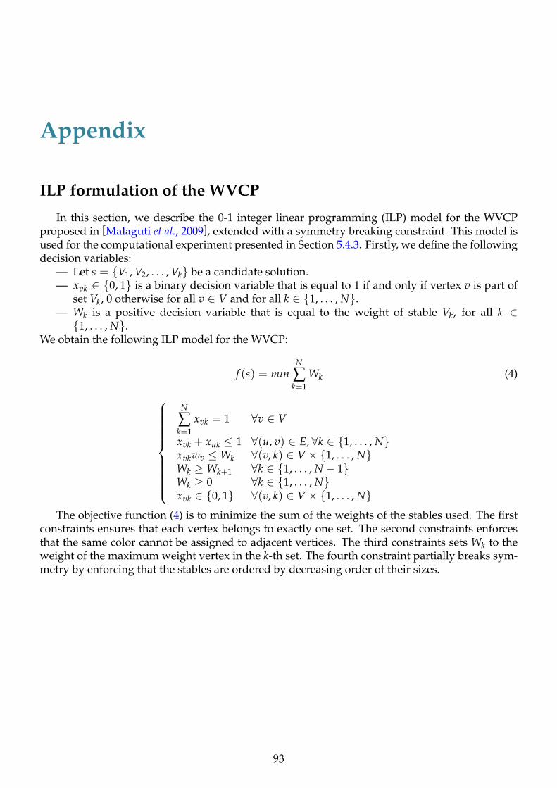
Appendix
ILP formulation of the WVCP
In this section, we describe the 0-1 integer linear programming (ILP) model for the WVCPproposed in [Malaguti et al., 2009], extended with a symmetry breaking constraint. This model isused for the computational experiment presented in Section 5.4.3. Firstly, we define the followingdecision variables:
— Let s = V1, V2, . . . , Vk be a candidate solution.— xvk ∈ 0, 1 is a binary decision variable that is equal to 1 if and only if vertex v is part of
set Vk, 0 otherwise for all v ∈ V and for all k ∈ 1, . . . , N.— Wk is a positive decision variable that is equal to the weight of stable Vk, for all k ∈1, . . . , N.
We obtain the following ILP model for the WVCP:
f (s) = minN
∑k=1
Wk (4)
N
∑k=1
xvk = 1 ∀v ∈ V
xvk + xuk ≤ 1 ∀(u, v) ∈ E, ∀k ∈ 1, . . . , Nxvkwv ≤Wk ∀(v, k) ∈ V × 1, . . . , NWk ≥Wk+1 ∀k ∈ 1, . . . , N − 1Wk ≥ 0 ∀k ∈ 1, . . . , Nxvk ∈ 0, 1 ∀(v, k) ∈ V × 1, . . . , N
The objective function (4) is to minimize the sum of the weights of the stables used. The firstconstraints ensures that each vertex belongs to exactly one set. The second constraints enforcesthat the same color cannot be assigned to adjacent vertices. The third constraints sets Wk to theweight of the maximum weight vertex in the k-th set. The fourth constraint partially breaks sym-metry by enforcing that the stables are ordered by decreasing order of their sizes.
93


List of Publications
Published/accepted journal papers1. Wen Sun, Jin-Kao Hao, and Alexandre Caminada. Iterated backtrack removal search for
finding k-vertex-critical subgraphs. Journal of Heuristics, pages 1-26, 2018.
2. Wen Sun, Jin-Kao Hao, Xiangjing Lai and Qinghua Wu. Adaptive feasible and infeasibletabu search for weighted vertex coloring. Information Sciences, 466: 203-219,2018.
Published/accepted conference papers1. Wen Sun, Jin-Kao Hao, Xiangjing Lai, Qinghua Wu. On feasible and infeasible search for
equitable graph coloring. In Proceedings of the Genetic and Evolutionary ComputationConference, pages 369-376. ACM, 2017.
95


List of Figures
1.1 A graph and its a 3-coloring solution . . . . . . . . . . . . . . . . . . . . . . . . . . 121.2 An example of equitable coloring of a graph . . . . . . . . . . . . . . . . . . . . . . 151.3 A graph, a feasible solution, an optimal solution . . . . . . . . . . . . . . . . . . . . 171.4 An example for the 4-vertex-critical subgraph. . . . . . . . . . . . . . . . . . . . . . 20
2.1 Flow chart of RMA algorithm for solving the k-GCP. . . . . . . . . . . . . . . . . . . 252.2 The classes matching procedure by a complete bipartite graph H . . . . . . . . . . 282.3 two solutions for a graph coloring and its graph matching G
′. . . . . . . . . . . . . 29
2.4 two solution for a graph coloring and its coarsened graph G′
. . . . . . . . . . . . 30
4.1 Influence of the increment/decrement value of the penalty efficient . . . . . . . . . 66
5.1 Flow chart of the iterated backtrack-based removal algorithm for finding k-VCS ina graph. . . . . . . . . . . . . . . . . . . . . . . . . . . . . . . . . . . . . . . . . . . . . 75
5.2 Removal procedure. . . . . . . . . . . . . . . . . . . . . . . . . . . . . . . . . . . . . . 775.3 Backtrack-based removal procedure. . . . . . . . . . . . . . . . . . . . . . . . . . . . 785.4 Perturbation procedure. . . . . . . . . . . . . . . . . . . . . . . . . . . . . . . . . . . 805.5 Update procedure. . . . . . . . . . . . . . . . . . . . . . . . . . . . . . . . . . . . . . 82
97


List of Tables
1.1 Integer programming formulations of graph coloring . . . . . . . . . . . . . . . . . 13
2.1 Settings of important parameters . . . . . . . . . . . . . . . . . . . . . . . . . . . . . 332.2 Comparative results of RMA with state-of-the-art algorithms MACOL and PLSCOL
on 19 easy benchmark instances. Improved upper bounds are indicated in bold. . . 352.3 Comparative results of RMA with state-of-the-art algorithms MACOL and PLSCOL
on 20 difficult benchmark instances. The best results are in bold. . . . . . . . . . . . 362.4 Assessment of different number of the parents. The better results are in bold. . . . 372.5 Assessment of different strategies. The better results are in bold. . . . . . . . . . . . 382.6 Analysis of the influence of the perturbation on the performance of the RMA algo-
rithm. The better results are in bold. . . . . . . . . . . . . . . . . . . . . . . . . . . . 38
3.1 Comparative results of FISA with state-of-the-art algorithms on the 73 benchmarkinstances. . . . . . . . . . . . . . . . . . . . . . . . . . . . . . . . . . . . . . . . . . . 50
3.2 Comparative results of the FISA algorithm with 3 different values of ϕ on the 26instances. The best results are in bold. . . . . . . . . . . . . . . . . . . . . . . . . . . 51
3.3 Analysis of the influence of the perturbation on the performance of the FISA algo-rithm. . . . . . . . . . . . . . . . . . . . . . . . . . . . . . . . . . . . . . . . . . . . . 51
4.1 Settings of important parameters . . . . . . . . . . . . . . . . . . . . . . . . . . . . . 614.2 Comparative results of AFISA with state-of-the-art algorithms on the 46 DIMACS
benchmark instances. Improved upper bounds are indicated in bold. . . . . . . . . 624.3 Comparative results of AFISA with state-of-the-art algorithms on the 35 pxx bench-
mark instances. Improved upper bounds are indicated in bold. . . . . . . . . . . . 634.4 Comparative results of AFISA with state-of-the-art algorithms on the 30 rxx bench-
mark instances. Improved upper bounds are indicated in bold. . . . . . . . . . . . 644.5 Comparative results of FISA with CPLEX on the additional set of 50 larger DI-
MACS/COLOR instances. Improved upper bounds are indicated in bold. . . . . . 644.6 Assessment of searching both feasible and infeasible solutions. The better results
are in bold. . . . . . . . . . . . . . . . . . . . . . . . . . . . . . . . . . . . . . . . . . . 674.7 Assessment of the perturbation strategy. The better results are in bold. . . . . . . . 68
5.1 Comparative results of IBR with state-of-the-art algorithm on the first category ofinstances. . . . . . . . . . . . . . . . . . . . . . . . . . . . . . . . . . . . . . . . . . . . 84
5.2 Comparative results of IBR with state-of-the-art algorithm on the second categoryof instances. . . . . . . . . . . . . . . . . . . . . . . . . . . . . . . . . . . . . . . . . . 84
5.3 Comparative results of IBR with state-of-the-art algorithm on the third category ofinstances. Improved results are indicated in bold. . . . . . . . . . . . . . . . . . . . 85
5.4 Comparative results of IBR with state-of-the-art algorithm on the fourth categoryof instances. Improved results are indicated in bold. . . . . . . . . . . . . . . . . . . 85
5.5 Comparative results of the IBR algorithm with two different backtrack strategies.Improved results are indicated in bold. . . . . . . . . . . . . . . . . . . . . . . . . . . 86
99

5.6 Analysis of the influence of the perturbation on the performance of the IBR algo-rithm. The BR algorithm is obtained by replacing the perturbation procedure of theIBR algorithm with a restart strategy. Improved results are indicated in bold. . . . 86
5.7 Influence of the backtracking procedure on the performance of the IBR algorithm.IR is obtained by disabling the backtracking procedure. Improved results are indi-cated in bold. . . . . . . . . . . . . . . . . . . . . . . . . . . . . . . . . . . . . . . . . 87
100
References
[Bahiense et al., 2014] Laura Bahiense, Yuri Frota, Thiago F. Noronha, and Celso C. Ribeiro. Abranch-and-cut algorithm for the equitable coloring problem using a formulation by represen-tatives. Discrete Applied Mathematics, 164:34–46, 2014. 16
[Barbosa et al., 2004] Valmir C. Barbosa, Carlos A.G. Assis, and Josina O. Do Nascimento. Twonovel evolutionary formulations of the graph coloring problem. Journal of Combinatorial Opti-mization, 8(1):41–63, 2004. 12, 13
[Barr et al., 1995] Richard S. Barr, Bruce L. Golden, James P. Kelly, Mauricio G.C. Resende, andWilliam R. Stewart. Designing and reporting on computational experiments with heuristicmethods. Journal of heuristics, 1(1):9–32, 1995. 62
[Benlic and Hao, 2011] Una Benlic and Jin-Kao Hao. A multilevel memetic approach for improv-ing graph k-partitions. IEEE Transactions on Evolutionary Computation, 15(5):624–642, 2011. 23,39
[Benlic and Hao, 2013] Una Benlic and Jin-Kao Hao. Breakout local search for maximum cliqueproblems. Computers & Operations Research, 40(1):192–206, 2013. 47, 59
[Bhasker and Samad, 1991] J. Bhasker and Tariq Samad. The clique-partitioning problem. Com-puters & Mathematics with Applications, 22(6):1–11, 1991. 13
[Blazewicz et al., 1997] Jacek Blazewicz, Klaus H Ecker, Erwin Pesch, Günter Schmidt, and JanWeglarz. Scheduling computer and manufacturing processes. Journal of the Operational ResearchSociety, 48(6):659–659, 1997. 15
[Blazewicz et al., 2013] Jacek Blazewicz, Klaus H. Ecker, Erwin Pesch, Günter Schmidt, and JanWeglarz. Scheduling computer and manufacturing processes. Springer Science & Business Media,2013.
[Blöchliger and Zufferey, 2008] Ivo Blöchliger and Nicolas Zufferey. A graph coloring heuristicusing partial solutions and a reactive tabu scheme. Computers & Operations Research, 35(3):960–975, 2008. 34, 35
[Bodlaender and Fomin, 2004] Hans L. Bodlaender and Fedor V. Fomin. Equitable colorings ofbounded treewidth graphs. In International Symposium on Mathematical Foundations of ComputerScience, pages 180–190. Springer, 2004. 15
[Bouhmala and Granmo, 2008] Noureddine Bouhmala and Ole-Christoffer Granmo. Solvinggraph coloring problems using learning automata. In European Conference on Evolutionary Com-putation in Combinatorial Optimization, pages 277–288. Springer, 2008. 14
[Brélaz, 1979] Daniel Brélaz. New methods to color the vertices of a graph. Communications of theACM, 22(4):251–256, 1979. 13, 33
[Burke et al., 1994] Edmund K. Burke, Elliman David, and Rupert Weare. A genetic algorithmbased university timetabling system. In Proceedings of the 2nd east-west international conferenceon computer technologies in education, volume 1, pages 35–40, 1994. 12
101

[Burke et al., 2010] Edmund K. Burke, Jakub Marecek, Andrew J. Parkes, and Hana Rudová. Asupernodal formulation of vertex colouring with applications in course timetabling. Annals ofOperations Research, 179(1):105–130, 2010. 13
[Campêlo et al., 2008] Manoel Campêlo, Victor A. Campos, and Ricardo C. Corrêa. On the asym-metric representatives formulation for the vertex coloring problem. Discrete Applied Mathemat-ics, 156(7):1097–1111, 2008. 13
[Campêlo et al., 2009] Manoel Campêlo, Victor A. Campos, and Ricardo C. Corrêa. Um algoritmode planos-de-corte para o número cromático fracionário de um grafo. Pesquisa Operacional,29(1):179–193, 2009. 13
[Caprara et al., 1999] Alberto Caprara, Matteo Fischetti, and Paolo Toth. A heuristic method forthe set covering problem. Operations Research, 47(5):730–743, 1999. 18
[Caramia and Dell Olmo, 2008] Massimiliano Caramia and Paolo Dell Olmo. Coloring graphs byiterated local search traversing feasible and infeasible solutions. Discrete Applied Mathematics,156(2):201–217, 2008. 34, 35
[Chaitin, 1982] Gregory J. Chaitin. Register allocation & spilling via graph coloring. In ACMSigplan Notices, volume 17, pages 98–105. ACM, 1982. 12
[Chakravarti, 1994] Nilotpal Chakravarti. Some results concerning post-infeasibility analysis. Eu-ropean Journal of Operational Research, 73(1):139–143, 1994.
[Chen and Hao, 2016] Yuning Chen and Jin-Kao Hao. Memetic search for the generalizedquadratic multiple knapsack problem. IEEE Transactions on Evolutionary Computation,20(6):908–923, 2016. 29, 39
[Chen et al., 1994] Bor-Liang Chen, Ko-Wei Lih, and Pou-Lin Wu. Equitable coloring and themaximum degree. European Journal of Combinatorics, 15(5):443–447, 1994. 15
[Chen et al., 2016a] Yuning Chen, Jin-Kao Hao, and Fred Glover. An evolutionary path relinkingapproach for the quadratic multiple knapsack problem. Knowledge-Based Systems, 92:23–34,2016. 52
[Chen et al., 2016b] Yuning Chen, Jin-Kao Hao, and Fred Glover. A hybrid metaheuristic ap-proach for the capacitated arc routing problem. European Journal of Operational Research,253(1):25–39, 2016. 19, 60, 90
[Chinneck and Dravnieks, 1991] John W. Chinneck and Erik W. Dravnieks. Locating minimalinfeasible constraint sets in linear programs. ORSA Journal on Computing, 3(2):157–168, 1991.72
[Chinneck, 1994] John W. Chinneck. Minos (iis): infeasibility analysis using minos. Computers &Operations Research, 21(1):1–9, 1994.
[Chinneck, 1997a] John W. Chinneck. Feasibility and viability. In Advances in Sensitivity Analysisand Parametic Programming, pages 491–531. Springer, 1997.
[Chinneck, 1997b] John W. Chinneck. Finding a useful subset of constraints for analysis in aninfeasible linear program. INFORMS Journal on Computing, 9(2):164–174, 1997. 72
[Coll et al., 2002] Pablo Coll, Javier Marenco, Isabel Méndez Díaz, and Paula Zabala. Facets of thegraph coloring polytope. Annals of Operations Research, 116(1-4):79–90, 2002. 12, 13
[Cornaz et al., 2017] Denis Cornaz, Fabio Furini, and Enrico Malaguti. Solving vertex coloringproblems as maximum weight stable set problems. Discrete Applied Mathematics, 217:151–162,2017. 18, 60, 61, 62, 63
[de Werra, 1985] Dominique de Werra. An introduction to timetabling. European journal of opera-tional research, 19(2):151–162, 1985. 12
102

[Desrosiers et al., 2008] Christian Desrosiers, Philippe Galinier, and Alain Hertz. Efficient algo-rithms for finding critical subgraphs. Discrete Applied Mathematics, 156(2):244–266, 2008. 19, 20,72, 75, 76, 81, 83, 84, 85
[Desrosiers et al., 2009] Christian Desrosiers, Philippe Galinier, Alain Hertz, and Sandrine Paroz.Using heuristics to find minimal unsatisfiable subformulas in satisfiability problems. Journal ofCombinatorial Optimization, 18(2):124–150, 2009.
[Díaz et al., 2014] Isabel Méndez Díaz, Graciela Nasini, and Daniel Severín. A tabu search heuris-tic for the equitable coloring problem. In International Symposium on Combinatorial Optimization,pages 347–358. Springer, 2014. 16, 43, 48
[Diaza et al., 2008] Isabel Méndez Diaza, Graciela Nasinib, and Daniel Severınb. A polyhedralapproach for the graph equitable coloring problem. 2008. 15
[Ding et al., 2015] Jian-Ya Ding, Shiji Song, Jatinder N.D. Gupta, Rui Zhang, Raymond Chiong,and Cheng Wu. An improved iterated greedy algorithm with a tabu-based reconstructionstrategy for the no-wait flowshop scheduling problem. Applied Soft Computing, 30:604–613,2015. 15
[Dorne and Hao, 1998] Raphaël Dorne and Jin-Kao Hao. A new genetic local search algorithmfor graph coloring. In International Conference on Parallel Problem Solving from Nature, pages745–754. Springer, 1998. 31
[Dorne and Hao, 1999] Raphaël Dorne and Jin-Kao Hao. Tabu search for graph coloring, t-colorings and set t-colorings. In Meta-heuristics, pages 77–92. Springer, 1999. 26, 76
[Edmund K. et al., 1994] Burke Edmund K., Elliman David, and Weare Rupert. A universitytimetabling system based on graph colouring and constraint manipulation. Journal of researchon computing in education, 27(1):1–18, 1994.
[Eisenberg and Faltings, 2003] Carlos Eisenberg and Boi Faltings. Using the breakout algo-rithm to identify hard and unsolvable subproblems. In Principles and Practice of ConstraintProgramming–CP 2003, pages 822–826. Springer, 2003. 20
[Elhag and Özcan, 2015] Anas Elhag and Ender Özcan. A grouping hyper-heuristic framework:Application on graph colouring. Expert Systems with Applications, 42(13):5491–5507, 2015. 14
[Fleurent and Ferland, 1996] Charles Fleurent and Jacques A. Ferland. Genetic and hybrid algo-rithms for graph coloring. Annals of Operations Research, 63(3):437–461, 1996. 14, 26
[Furini and Malaguti, 2012] Fabio Furini and Enrico Malaguti. Exact weighted vertex coloringvia branch-and-price. Discrete Optimization, 9(2):130–136, 2012. 18
[Furmanczyk and Kubale, 2004] Hanna Furmanczyk and Marek Kubale. Equitable coloring ofgraphs. Contemporary Mathematics, 352:35–54, 2004. 15, 16
[Furmanczyk and Kubale, 2005] Hanna Furmanczyk and Marek Kubale. The complexity of eq-uitable vertex coloring of graphs. Journal of Applied Computer Science, 13(2):95–106, 2005. 15
[Galinier and Hao, 1999] Philippe Galinier and Jin-Kao Hao. Hybrid evolutionary algorithms forgraph coloring. Journal of combinatorial optimization, 3(4):379–397, 1999. 14, 16, 23, 24, 25, 26, 31,34, 35, 57, 76
[Galinier and Hertz, 2006] Philippe Galinier and Alain Hertz. A survey of local search methodsfor graph coloring. Computers & Operations Research, 33(9):2547–2562, 2006. 12, 14, 19, 23, 57
[Galinier and Hertz, 2007] Philippe Galinier and Alain Hertz. Solution techniques for the largeset covering problem. Discrete Applied Mathematics, 155(3):312–326, 2007.
[Galinier et al., 2004] Philippe Galinier, Alain Hertz, and Nicolas Zufferey. An adaptive memoryalgorithm for the k-colouring problem. Groupe d’études et de recherche en analyse des décisions,HEC Montréal, 2004.
103

[Galinier et al., 2008] Philippe Galinier, Alain Hertz, and Nicolas Zufferey. An adaptive memoryalgorithm for the k-coloring problem. Discrete Applied Mathematics, 156(2):267–279, 2008. 33,34, 35
[Galinier et al., 2011] Philippe Galinier, Zied Boujbel, and Michael Coutinho Fernandes. An ef-ficient memetic algorithm for the graph partitioning problem. Annals of Operations Research,191(1):1–22, 2011. 39
[Galinier et al., 2013] Philippe Galinier, Jean-Philippe Hamiez, Jin-Kao Hao, and Daniel Porum-bel. Recent advances in graph vertex coloring. In Handbook of optimization, pages 505–528.Springer, 2013. 12, 19, 23, 33, 43
[Gamst, 1986] Andreas Gamst. Some lower bounds for a class of frequency assignment problems.IEEE transactions on vehicular technology, 35(1):8–14, 1986. 12
[Garey and Johnson, 1979] Michael R. Garey and David S. Johnson. Computers and intractability:a guide to the theory of np-completeness. 1979. San Francisco, LA: Freeman, 58, 1979. 12, 23
[Gavranovic and Finke, 2000] H. Gavranovic and G. Finke. Graph partitioning and set coveringfor the optimal design of a production system in the metal industry. IFAC Proceedings Volumes,33(17):603–608, 2000. 18
[Glover and Hao, 2011] Fred Glover and Jin-Kao Hao. The case for strategic oscillation. Annals ofOperations Research, 183(1):163–173, 2011. 17, 19, 52, 90
[Glover and Laguna, 2013] Fred Glover and Manuel Laguna. Tabu search. In Handbook of Combi-natorial Optimization, pages 3261–3362. Springer, 2013. 45
[Glover et al., 1996] Fred Glover, Mark Parker, and Jennifer Ryan. Coloring by tabu branch andbound. DIMACS Series in Discrete Mathematics and Theoretical Computer Science, 26:285–307,1996. 24, 25
[Glover et al., 2010] Fred Glover, Zhipeng Lü, and Jin-Kao Hao. Diversification-driven tabusearch for unconstrained binary quadratic problems. 4OR, 8(3):239–253, 2010. 78
[Glover, 1989] Fred Glover. Tabu search-part i. ORSA Journal on computing, 1(3):190–206, 1989. 8,57
[Glover, 1990] Fred Glover. Tabu search-part ii. ORSA Journal on computing, 2(1):4–32, 1990. 8, 57[Glover, 1997] Fred Glover. Manuel laguna: Tabu search, 1997. 54, 57[Guo et al., 2018] Jianding Guo, Laurent Moalic, Jean-Noel Martin, and Alexandre Caminada. Ex-
act graph coloring algorithms of getting partial and all best solutions. In ISAIM, 2018. 13[Gusfield, 2002] Dan Gusfield. Partition-distance: A problem and class of perfect graphs arising
in clustering. Information Processing Letters, 82(3):159–164, 2002. 32[Hale, 1980] William K. Hale. Frequency assignment: Theory and applications. Proceedings of the
IEEE, 68(12):1497–1514, 1980. 12[Hamida and Schoenauer, 2000] S. Ben Hamida and Marc Schoenauer. An adaptive algorithm for
constrained optimization problems. In International Conference on Parallel Problem Solving fromNature, pages 529–538. Springer, 2000. 58
[Hansen et al., 2009] Pierre Hansen, Martine Labbé, and David Schindl. Set covering and packingformulations of graph coloring: Algorithms and first polyhedral results. Discrete Optimization,6(2):135–147, 2009. 12, 13
[Hao and Wu, 2012] Jin-Kao Hao and Qinghua Wu. Improving the extraction and expansionmethod for large graph coloring. Discrete Applied Mathematics, 160(16-17):2397–2407, 2012. 14
[Hao, 2012] Jin-Kao Hao. Memetic algorithms in discrete optimization. In Handbook of memeticalgorithms, pages 73–94. Springer, 2012.
104

[Herrmann and Hertz, 2002] Francine Herrmann and Alain Hertz. Finding the chromatic num-ber by means of critical graphs. Journal of Experimental Algorithmics, 7:10, 2002. 19, 20, 72
[Hertz and de Werra, 1987] Alain Hertz and Dominique de Werra. Using tabu search techniquesfor graph coloring. Computing, 39(4):345–351, 1987. 14, 16, 57, 76
[Hertz et al., 2008] Alain Hertz, Matthieu Plumettaz, and Nicolas Zufferey. Variable space searchfor graph coloring. Discrete Applied Mathematics, 156(13):2551–2560, 2008. 34, 35
[Hochbaum and Landy, 1997] Dorit S. Hochbaum and Dan Landy. Scheduling semiconductorburn-in operations to minimize total flowtime. Operations Research, 45(6):874–885, 1997. 18
[Hu et al., 2011] Jun Hu, Philippe Galinier, and Alexandre Caminada. Yet another breakout in-spired infeasible subset detection in constraint satisfaction problem. In Proceedings on the Inter-national Conference on Artificial Intelligence (ICAI), page 1. The Steering Committee of The WorldCongress in Computer Science, Computer Engineering and Applied Computing (WorldComp),2011. 19
[Irani and Leung, 1996] Sandy Irani and Vitus Leung. Scheduling with conflicts, and applicationsto traffic signal control. In SODA, volume 96, pages 85–94, 1996. 15
[Jin and Hao, 2016] Yan Jin and Jin-Kao Hao. Hybrid evolutionary search for the minimum sumcoloring problem of graphs. Information Sciences, 352:15–34, 2016. 19, 57
[Johnson et al., 1989] David S. Johnson, Cecilia R. Aragon, Lyle A. McGeoch, and CatherineSchevon. Optimization by simulated annealing: an experimental evaluation; part i, graphpartitioning. Operations Research, 37(6):865–892, 1989.
[Kitagawa and Ikeda, 1988] Fumio Kitagawa and Hideto Ikeda. An existential problem of aweightcontrolled subset and its application to school timetable construction. In Annals of Dis-crete Mathematics, volume 38, pages 195–211. Elsevier, 1988. 15
[Kostochka and Nakprasit, 2005] Alexandr V. Kostochka and Kittikorn Nakprasit. On equitableδ-coloring of graphs with low average degree. Theoretical Computer Science, 349(1):82–91, 2005.15
[Kostochka, 2002] Alexandr V. Kostochka. Equitable colorings of outerplanar graphs. DiscreteMathematics, 258(1-3):373–377, 2002. 15
[Kuhn, 1955] Harold W. Kuhn. The hungarian method for the assignment problem. Naval Re-search Logistics (NRL), 2(1-2):83–97, 1955. 29
[Lai et al., 2015] Xiangjing Lai, Jin-Kao Hao, and Fred Glover. Backtracking based iterated tabusearch for equitable coloring. Engineering Applications of Artificial Intelligence, 46:269–278, 2015.16, 42, 43, 45, 46, 47, 48, 57, 89
[Lai et al., 2018] Xiangjing Lai, Jin-Kao Hao, Fred Glover, and Zhipeng Lü. A two-phase tabu-evolutionary algorithm for the 0–1 multidimensional knapsack problem. Information Sciences,436:282–301, 2018. 19
[Lee and Margot, 2007] Jon Lee and François Margot. On a binary-encoded ilp coloring formula-tion. INFORMS Journal on Computing, 19(3):406–415, 2007. 12
[Lee, 2002] Jon Lee. All-different polytopes. Journal of Combinatorial Optimization, 6(3):335–352,2002. 12, 13
[Leighton, 1979] Frank Thomson Leighton. A graph coloring algorithm for large schedulingproblems. Journal of research of the national bureau of standards, 84(6):489–506, 1979. 12, 13
[Lewis, 2015] Rhyd Lewis. A Guide to Graph Colouring. Springer, 2015. 7[Li and Huang, 2005] Chu Min Li and Wen Qi Huang. Diversification and determinism in lo-
cal search for satisfiability. In Theory and Applications of Satisfiability Testing, pages 158–172.Springer, 2005.
105

[Liffiton and Sakallah, 2005] Mark H. Liffiton and Karem A. Sakallah. On finding all minimallyunsatisfiable subformulas. In International Conference on Theory and Applications of SatisfiabilityTesting, pages 173–186. Springer, 2005.
[Lih and Wu, 1996] Ko-Wei Lih and Pou-Lin Wu. On equitable coloring of bipartite graphs. Dis-crete Mathematics, 151(1-3):155–160, 1996. 15
[Lin, 1993] Nai-Wei Lin. Approximating the chromatic polynomial of a graph. In InternationalWorkshop on Graph-Theoretic Concepts in Computer Science, pages 200–210. Springer, 1993. 13
[Lin, 2013] Chih-Hao Lin. A rough penalty genetic algorithm for constrained optimization. In-formation Sciences, 241:119–137, 2013. 19
[Lü and Hao, 2009] Zhipeng Lü and Jin-Kao Hao. A critical element-guided perturbation strat-egy for iterated local search. In Evolutionary Computation in Combinatorial Optimization, pages1–12. Springer, 2009. 78
[Lü and Hao, 2010] Zhipeng Lü and Jin-Kao Hao. A memetic algorithm for graph coloring. Eu-ropean Journal of Operational Research, 203(1):241–250, 2010. 14, 23, 25, 27, 32, 33, 34, 35
[Lucet et al., 2006] Corinne Lucet, Florence Mendes, and Aziz Moukrim. An exact method forgraph coloring. Computers & operations research, 33(8):2189–2207, 2006. 13
[Mahmoudi and Lotfi, 2015] Shadi Mahmoudi and Shahriar Lotfi. Modified cuckoo optimizationalgorithm (mcoa) to solve graph coloring problem. Applied soft computing, 33:48–64, 2015. 14
[Malaguti and Toth, 2010] Enrico Malaguti and Paolo Toth. A survey on vertex coloring prob-lems. International transactions in operational research, 17(1):1–34, 2010. 12, 19, 57
[Malaguti et al., 2008] Enrico Malaguti, Michele Monaci, and Paolo Toth. A metaheuristic ap-proach for the vertex coloring problem. INFORMS Journal on Computing, 20(2):302–316, 2008.23, 34, 35
[Malaguti et al., 2009] Enrico Malaguti, Michele Monaci, and Paolo Toth. Models and heuristicalgorithms for a weighted vertex coloring problem. Journal of Heuristics, 15(5):503–526, 2009.18, 54, 60, 61, 62, 63, 65, 93
[Malaguti et al., 2011] Enrico Malaguti, Michele Monaci, and Paolo Toth. An exact approach forthe vertex coloring problem. Discrete Optimization, 8(2):174–190, 2011. 13, 14
[Malaguti, 2009] Enrico Malaguti. The vertex coloring problem and its generalizations. PhD thesis,Springer, 2009. 18
[Martin, 2010] Jean-Noel Martin. No Free Lunch et recherche de solutions structurantes en coloration.PhD thesis, Université de Technologie de Belfort-Montbeliard, 2010. 13
[Martinez-Gavara et al., 2017] Anna Martinez-Gavara, Dario Landa-Silva, Vicente Campos, andRafael Marti. Randomized heuristics for the capacitated clustering problem. Information Sci-ences, 417:154–168, 2017. 19, 60
[Mehrotra and Trick, 1996] Anuj Mehrotra and Michael A. Trick. A column generation approachfor graph coloring. informs Journal on Computing, 8(4):344–354, 1996. 12, 13
[Méndez-Díaz and Zabala, 2006] Isabel Méndez-Díaz and Paula Zabala. A branch-and-cut algo-rithm for graph coloring. Discrete Applied Mathematics, 154(5):826–847, 2006. 12, 13
[Méndez-Díaz and Zabala, 2008] Isabel Méndez-Díaz and Paula Zabala. A cutting plane algo-rithm for graph coloring. Discrete Applied Mathematics, 156(2):159–179, 2008. 12, 13
[Méndez-Díaz et al., 2014] Isabel Méndez-Díaz, Graciela Nasini, and Daniel Severín. A polyhe-dral approach for the equitable coloring problem. Discrete Applied Mathematics, 164:413–426,2014. 16, 48, 49
106

[Méndez-Díaz et al., 2015] Isabel Méndez-Díaz, Graciela Nasini, and Daniel Severín. A dsatur-based algorithm for the equitable coloring problem. Computers & Operations Research, 57:41–50,2015. 16, 48, 49
[Meyer, 1973] Walter Meyer. Equitable coloring. The American Mathematical Monthly, 80(8):920–922, 1973. 15
[Michael and David, 1979] R. Garey Michael and S. Johnson David. Computers and intractability:a guide to the theory of np-completeness. W.H. Free. Co., San Fr, pages 90–91, 1979. 18
[Michalewicz and Schoenauer, 1996] Zbigniew Michalewicz and Marc Schoenauer. Evolutionaryalgorithms for constrained parameter optimization problems. Evolutionary computation, 4(1):1–32, 1996. 46
[Mneimneh et al., 2005] Maher Mneimneh, Inês Lynce, Zaher Andraus, João Marques-Silva, andKarem Sakallah. A branch-and-bound algorithm for extracting smallest minimal unsatisfiableformulas. In International Conference on Theory and Applications of Satisfiability Testing, pages467–474. Springer, 2005.
[Moalic and Gondran, 2015] Laurent Moalic and Alexandre Gondran. The new memetic algo-rithm head for graph coloring: An easy way for managing diversity. In European Conference onEvolutionary Computation in Combinatorial Optimization, pages 173–183. Springer, 2015. 14, 23,34, 35
[Morgenstern, 1996] Craig Morgenstern. Distributed coloration neighborhood search. DiscreteMathematics and Theoretical Computer Science, 26:335–358, 1996.
[Moscato and Cotta, 2003] Pablo Moscato and Carlos Cotta. A gentle introduction to memeticalgorithms. In Handbook of metaheuristics, pages 105–144. Springer, 2003.
[Neri et al., 2012] Ferrante Neri, Carlos Cotta, and Pablo Moscato. Handbook of memetic algorithms,volume 379. Springer, 2012.
[Nicholson, 1998] Mark Nicholson. Genetic algorithms and grouping problems, 1998. 39[Oh et al., 2004] Yoonna Oh, Maher N. Mneimneh, Zaher S. Andraus, Karem A. Sakallah, and
Igor L. Markov. Amuse: a minimally-unsatisfiable subformula extractor. In Proceedings of the41st annual Design Automation Conference, pages 518–523. ACM, 2004.
[Porumbel et al., 2010] Daniel Cosmin Porumbel, Jin-Kao Hao, and Pascale Kuntz. An evolution-ary approach with diversity guarantee and well-informed grouping recombination for graphcoloring. Computers & Operations Research, 37(10):1822–1832, 2010. 14, 23, 34, 35
[Prais and Ribeiro, 2000] Marcelo Prais and Celso C. Ribeiro. Reactive grasp: An application toa matrix decomposition problem in tdma traffic assignment. INFORMS Journal on Computing,12(3):164–176, 2000. 18, 54, 55, 60, 61, 62, 63, 65
[Rao, 2004] Michaël Rao. Coloring a graph using split decomposition. In International Workshopon Graph-Theoretic Concepts in Computer Science, pages 129–141. Springer, 2004. 13
[Read, 1968] Ronald C. Read. An introduction to chromatic polynomials. Journal of CombinatorialTheory, 4(1):52–71, 1968. 13
[Ribeiro et al., 1989] Celso Carneiro Ribeiro, Michel Minoux, and Manoel Camillo Penna. An op-timal column-generation-with-ranking algorithm for very large scale set partitioning problemsin traffic assignment. European Journal of Operational Research, 41(2):232–239, 1989. 18
[San Segundo, 2012] Pablo San Segundo. A new dsatur-based algorithm for exact vertex coloring.Computers & Operations Research, 39(7):1724–1733, 2012.
[Schaerf, 2003] D.G. Schaerf. Multi neighborhood local search with application to the coursetimetabling problem. In Proceedings of the 4th International Conference on Practice and Theoryof Automated Timetabling (PATAT-2002), 2003.
107
[Schindl, 2004] David Schindl. Some combinatorial optimization problems in graphs with appli-cations in telecommunications and tomography. 2004. 12
[Sghir et al., 2015] Ines Sghir, Jin-Kao Hao, Ines Ben Jaafar, and Khaled Ghédira. A multi-agentbased optimization method applied to the quadratic assignment problem. Expert Systems withApplications, 42(23):9252–9262, 2015. 14
[Sun et al., 2017] Wen Sun, Jin-Kao Hao, Xiangjing Lai, and Qinghua Wu. On feasible and infeasi-ble search for equitable graph coloring. In Proceedings of the Genetic and Evolutionary ComputationConference, pages 369–376. ACM, 2017. 19, 41, 57, 60
[Sun et al., 2018a] Wen Sun, Jin-Kao Hao, and Alexandre Caminada. Iterated backtrack removalsearch for finding k-vertex-critical subgraphs. Journal of Heuristics, pages 1–26, 2018. 71
[Sun et al., 2018b] Wen Sun, Jin-Kao Hao, Xiangjing Lai, and Qinghua Wu. Adaptive feasible andinfeasible tabu search for weighted vertex coloring. Information Sciences, 466:203–219, 2018. 53
[Tamiz et al., 1996] Mehrdad Tamiz, Simon J. Mardle, and Dylan F. Jones. Detecting iis in infea-sible linear programmes using techniques from goal programming. Computers & OperationsResearch, 23(2):113–119, 1996.
[Titiloye and Crispin, 2011] Olawale Titiloye and Alan Crispin. Quantum annealing of the graphcoloring problem. Discrete Optimization, 8(2):376–384, 2011. 14, 34, 35
[Titiloye and Crispin, 2012] Olawale Titiloye and Alan Crispin. Parameter tuning patterns forrandom graph coloring with quantum annealing. PloS one, 7(11):e50060, 2012. 34, 35
[Tucker, 1973] Alan Tucker. Perfect graphs and an application to optimizing municipal services.Siam Review, 15(3):585–590, 1973. 15
[Van Loon, 1981] J.N.M. Van Loon. Irreducibly inconsistent systems of linear inequalities. Euro-pean Journal of Operational Research, 8(3):283–288, 1981.
[Walshaw, 2004] Chris Walshaw. Multilevel refinement for combinatorial optimisation problems.Annals of Operations Research, 131(1-4):325–372, 2004. 23
[Wang et al., 2018] Wenyu Wang, Jin-Kao Hao, and Qinghua Wu. Tabu search with feasible andinfeasible searches for equitable coloring. Engineering Applications of Artificial Intelligence, 71:1–14, 2018. 16, 19, 57, 60
[Williams and Yan, 2001] H. Paul Williams and Hong Yan. Representations of the all_differentpredicate of constraint satisfaction in integer programming. INFORMS Journal on Computing,13(2):96–103, 2001. 12, 13
[Wu and Hao, 2013] Qinghua Wu and Jin-Kao Hao. A hybrid metaheuristic method for the max-imum diversity problem. European Journal of Operational Research, 231(2):452–464, 2013. 14
[Yan and Wang, 2014] Zhidan Yan and Wei Wang. Equitable coloring of kronecker products ofcomplete multipartite graphs and complete graphs. Discrete Applied Mathematics, 162:328–333,2014. 15
[Zhang and Malik, 2003] Lintao Zhang and Sharad Malik. Extracting small unsatisfiable coresfrom unsatisfiable boolean formula. SAT, 3, 2003.
[Zhou et al., 2014] Zhaoyang Zhou, Chu-Min Li, Chong Huang, and Ruchu Xu. An exact algo-rithm with learning for the graph coloring problem. Computers & Operations Research, 51:282–301, 2014. 13, 14, 83
[Zhou et al., 2018] Yangming Zhou, Béatrice Duval, and Jin-Kao Hao. Improving probabilitylearning based local search for graph coloring. Applied Soft Computing, 65:542–553, 2018. 14, 34,35
108

[Zufferey et al., 2008] Nicolas Zufferey, Patrick Amstutz, and Philippe Giaccari. Graph colouringapproaches for a satellite range scheduling problem. Journal of Scheduling, 11(4):263–277, 2008.12
109


Titre : Algorithmes heuristiques pour des problèmes de coloration de graphes
................... ............................ ............................................................. ............................
Mots clés : Optimisation combinatoire, Problèmes de coloration de graphes, Recherche mixte réalisable et irréalisable, Heuristiques et métaheuristiques.
Résumé : Cette thèse concerne quatre problèmes de coloration de graphes NP-difficiles, à savoir le problème de coloration (GCP), le problème de coloration équitable (ECP), le problème de coloration des sommets pondérés et le problème de sous-graphe critique (k-VCS). Ces problèmes sont largement étudiés dans la littérature, non seulement pour leur difficulté théorique, mais aussi pour leurs applications réelles dans de nombreux domaines. Étant donné qu'ils appartiennent à la classe de problèmes NP-difficiles, il est difficile de les résoudre dans le cas général de manière exacte.
Pour cette raison, cette thèse est consacrée au développement d'approches heuristiques pour aborder ces problèmes complexes. Plus précisément, nous développons un algorithme mémétique de réduction (RMA) pour la coloration des graphes, un algorithme de recherche réalisable et irréalisable (FISA) pour la coloration équitable et un réalisable et irréalisable (AFISA) pour le problème de coloration des sommets pondérés et un algorithme de suppression basé sur le retour en arrière (IBR) pour le problème k-VCS. Tous les algorithmes ont été expérimentalement évalués et comparés aux méthodes de l'état de l'art.
Title : Heuristic Algorithms for Graph Coloring Problems
.................... ............................ ............................................................. ............................
Keywords : Combinatorial optimization, Graph coloring problems, Feasible and infeasible search strategies, Heuristics and metaheuristics.
Abstract : This thesis concerns four NP-hard graph coloring problems, namely, graph coloring (GCP), equitable coloring (ECP), weighted vertex coloring (WVCP) and k-vertex-critical subgraphs (k-VCS). These problems are extensively studied in the literature not only for their theoretical intractability, but also for their real-world applications in many domains. Given that they belong to the class of NP-hard problems, it is computationally difficult to solve them exactly in the general case.
For this reason, this thesis is devoted to developing effective heuristic approaches to tackle these challenging problems. We develop a reduction memetic algorithm (RMA) for the graph coloring problem, a feasible and infeasible search algorithm (FISA) for the equitable coloring problem, an adaptive feasible and infeasible search algorithm (AFISA) for the weighted vertex coloring problem and an iterated backtrack-based removal (IBR) algorithm for the k-VCS problem. All these algorithms were experimentally evaluated and compared with state-of-the-art methods.