a comparison of environmental substrate gradients and

University of Massachusetts Amherst University of Massachusetts Amherst

ScholarWorks@UMass Amherst ScholarWorks@UMass Amherst

Masters Theses 1911 - February 2014

January 2008

A Comparison of Environmental Substrate Gradients and Calcium A Comparison of Environmental Substrate Gradients and Calcium

Selectivity in Plant Species of Calcareous Fens in Massachusetts Selectivity in Plant Species of Calcareous Fens in Massachusetts

Jamie M. Morgan University of Massachusetts Amherst

Follow this and additional works at: https://scholarworks.umass.edu/theses

Morgan, Jamie M., "A Comparison of Environmental Substrate Gradients and Calcium Selectivity in Plant Species of Calcareous Fens in Massachusetts" (2008). Masters Theses 1911 - February 2014. 123. Retrieved from https://scholarworks.umass.edu/theses/123

This thesis is brought to you for free and open access by ScholarWorks@UMass Amherst. It has been accepted for inclusion in Masters Theses 1911 - February 2014 by an authorized administrator of ScholarWorks@UMass Amherst. For more information, please contact [email protected].

https://scholarworks.umass.edu/

https://scholarworks.umass.edu/theses

https://scholarworks.umass.edu/theses?utm_source=scholarworks.umass.edu%2Ftheses%2F123&utm_medium=PDF&utm_campaign=PDFCoverPages

https://scholarworks.umass.edu/theses/123?utm_source=scholarworks.umass.edu%2Ftheses%2F123&utm_medium=PDF&utm_campaign=PDFCoverPages

mailto:[email protected]

i

i

A COMPARISON OF ENVIRONMENTAL SUBSTRATE GRADIENTS AND

CALCIUM SELECTIVITY IN PLANT SPECIES OF CALCAREOUS FENS IN

MASSACHUSETTS

A Thesis Presented

by

JAMIE MARIE MORGAN

Submitted to the Graduate School of the University of Massachusetts Amherst in partial fulfillment

of the requirements for the degree of

MASTER OF SCIENCE

May 2008

Department of Plant, Soil, and Insect Sciences

ii

© Copyright by Jamie Marie Morgan 2008

All Rights Reserved

iii


CALCIUM SELECTIVITY IN PLANT SPECIES OF CALCAREOUS FENS IN

MASSACHUSETTS

A Thesis Presented

by

JAMIE MARIE MORGAN

Approved as to style and content by: _______________________________ Peter L. M. Veneman, Chair _______________________________ Lynn Adler, Member _______________________________ Allen V. Barker, Member _______________________________ Deborah J. Picking, Member

___________________________________

Peter L. M. Veneman, Department Head Department of Plant, Soil, and Insect Sciences

iv

DEDICATION

To my parents, Karen-Marie and Arthur Morgan, and to my grandpa, Trygve Stange, for their endless encouragement and support, and for teaching me the value of hard work.

v

“Wherever the reign of nature is not disturbed by human interference, the different plant-species join together in communities, each of which has a characteristic form, and constitutes a feature in the landscape of which it is a part. These communities are distributed and grouped together in a great variety of ways, and, like the lines on a man’s face, they give a particular impress to the land where they grow. The species of which a community is composed may belong to the most widely different natural groups of plants. The reason for their living together does not lie in their being of common origin, but in the nature of the habitat. They are forced into companionship not by any affinity to one another but by the fact that their vital necessities are the same… A knowledge of the communities which exist within the realm of plants is of great importance in many ways. It throws a strong light, not only on the mutual relations of the different species which are associated by common or similar needs, but also on the connection of plant-life with local and climatic conditions and with the nature of the soil. It may fairly be said that in the various zones and regions of our earth no kind of phenomenon so thoroughly gives expression to the climate and the constitution of the soil as the presence of particular plant-communities which prevail, and, accordingly, the determination and description of such communities constitutes an important part of geography.” - Anton Kerner Von Marilaun, from The Natural History of Plants, 1895

vi

ACKNOWLEDGEMENTS

First I must thank my committee members: Dr. Deb Picking for her zestful interest in the subject matter and for the exceptional guidance she provided me in every aspect of this work; Dr. Peter Veneman for providing me with laboratory space, financial support, and a fascinating understanding of soil morphology; Dr. Allen Barker for teaching me the joy of plant nutrition; and Dr. Lynn Adler for assisting me with the arduous task of analyzing my data and for her unique approach to teaching statistics and experimental design. A special thanks to Dr. Stephen Simkins for his patience in answering my detailed questions and to Sarah Weis for so nicely and patiently assisting me with many of the analytical procedures I used for this research. I am also grateful to Steven Bodine and everyone at the UMass Soil Testing lab for assisting me with analyses and allowing me to use their instruments. Thanks to Jess Murray Toro and Angela Sirois from the Nature Conservancy in Sheffield, Massachusetts, for permitting me into their wetlands even though they are habitat for the endangered Bog Turtle and providing me with accommodations at their Berkshire field station. Thanks also to Mike Allen for assisting me in the field on his time off and for his overall companionship. Much thanks to the Society of Soil Scientists of Southern New England for their financial assistance. Finally, I would like to thank my professors at Rutgers: Dr. Roger Locandro for introducing me to “limestone species” and Dr. Colleen Hatfield for her continuous support and encouragement. Thank You!

vii

ABSTRACT


CALCIUM SELECTIVITY IN PLANT SPECIES OF CALCAREOUS FENS OF

MASSACHUSETTS

May 2008

JAMIE MARIE MORGAN, B.A., RUTGERS UNIVERSITY

M.S., UNIVERSITY OF MASSACHUSETTS AMHERST

Directed by: Dr. Deborah J. Picking

The distribution and occurrence of plant species within a given region provides

insight into the many environmental properties of that region. Although much research

has been conducted on plant communities and associated environmental properties, few

studies have been conducted on the characteristics of individual plants within those

communities. Calcareous fens are wetlands formed by the upwelling of mineral-rich

groundwater and often are associated with many unique plant communities and rare

species of flora and fauna. Although many studies have documented the vegetation

patterns and associated environmental gradients of these fens, none have isolated the

specific hydrogeochemical conditions associated with individual species, nor have any

studies attempted to document and compare the individual physiological response of

species to elevated environmental calcium levels. This research was conducted to

estimate environmental calcium requirements for rare as well as common indicator

species of calcareous fens of Massachusetts and to examine the relationship between the

accumulation of calcium in the tissues of these species to calcium availability in their

viii

environment. These factors will be important when determining required conditions for

fen restoration and will further the understanding of why these species often only occur in

calcareous fens.

Eight calcareous fen study sites at three different locations were established where

calciphiles occur in western Massachusetts. In each site, data were collected on the

vegetation patterns and associated soil chemistry, water chemistry, and hydrology. In

addition, plant tissues were collected and analyzed for calcium. Species distributions

were evaluated as to whether they increased in abundance as environmental calcium did

or whether they appeared to occur only once a specific calcium threshold was met. In

addition, the concentrations of calcium in the tissues were used to determine the extent to

which those plants accumulated calcium and how those levels related to levels of calcium

in the substrate environment and to their overall distributions.

It was found that certain calciphiles are calcium specialists, i.e. they are more

abundant when environmental calcium levels are elevated, absorb greater quantities of

calcium and those quantities correlate to the available environmental supply. These

species include Parnassia glauca, Packera aurea, Geum rivale and Carex granularis. Of

these, Geum rivale and Carex granularis, as well as Carex sterilis, did not occur below

calcium concentrations of 48 mg.L-1. However, other calciphiles are calcium generalists,

i.e. they are tolerant of elevated calcium levels but show no other relationship with

respect to growth or accumulation. These species include Carex flava, Carex hystericina,

Juncus nodosus, Solidago patula, Solidago uliginosa, and Symphyotrichum puniceum. In

addition, some wetland generalists maintain elevated calcium levels (Symplocarpus

foetidus and Mentha arvensis) whereas most others do not (Thelypteris palustris and

ix

Fragaria vesca). Of the calciphile and wetland generalist species, some appear to

increase in abundance in calcareous fens in relation to increases in accessory benefits

(Dasiphora fruticosa and Juncus brachycephalus with pH; Thelypteris palustris and

Carex flava with magnesium and possibly Equisetum fluviatile with iron). Combined,

these findings characterize the growth habits and calcium accumulation of species that

grow in calcareous fens and indicate that calciphiles have varying degrees of dependence

on calcium.

x

TABLE OF CONTENTS Page

ACKNOWLEDGEMENTS ........................................................................................... vi ABSTRACT ................................................................................................................... vii LIST OF TABLES ......................................................................................................... xiv LIST OF FIGURES ..................................................................................................... xviii CHAPTER I. INTRODUCTION ..................................................................................................... 1 Justification .............................................................................................................. 2 Hypothesis................................................................................................................ 4 Objectives ................................................................................................................ 4 Study Site Layout ..................................................................................................... 5

Hydrogeochemical Setting ................................................................................. 7 II. LITERATURE REVIEW ......................................................................................... 13 Wetland Hydrology .................................................................................................. 13 Fen Geochemistry .................................................................................................... 14 Fen Plant Communities ............................................................................................ 16 Calcium in Plants ..................................................................................................... 17 Fen Plant Nutrition ................................................................................................... 20 Calcium Uptake ....................................................................................................... 20 Calcium and Plant Ecology ...................................................................................... 22 Habitat Conservation ............................................................................................... 23 III. HYDROLOGY, GEOCHEMISTRY, AND SOILS ............................................... 26 Introduction .............................................................................................................. 26 Materials and Methods ............................................................................................. 27

Hydrologic Measurements ................................................................................. 27 Water Chemical Analysis .................................................................................. 27 Soil Analysis ...................................................................................................... 29 Data Analysis ..................................................................................................... 29

Results and Discussion ............................................................................................ 30

Hydrologic Measurements ................................................................................. 30

xi

Page

Well Data ..................................................................................................... 30 Piezometer Data ........................................................................................... 33 Redoximorphic Conditions .......................................................................... 35

Water Chemical Analyses .................................................................................. 35

pH ................................................................................................................. 35 Calcium and Magnesium ............................................................................. 36 Iron ............................................................................................................... 46 Potassium ..................................................................................................... 49 Ammonium and Orthophosphate ................................................................. 51

Soil Analysis ...................................................................................................... 53

Soil Physical Properties ............................................................................... 53 Soil Chemical Properties .............................................................................. 55

General Chemical Properties ............................................................................. 58 Hydrology – Geochemistry Relationships ......................................................... 59

Conclusions .............................................................................................................. 61 IV. PLANT COMMUNITY ANALYSIS ..................................................................... 63 Introduction .............................................................................................................. 63 Materials and Methods ............................................................................................. 64

Vegetation Survey .............................................................................................. 64 A Priori Species Selection ................................................................................. 64 Species Richness and Turnover ......................................................................... 65


Community Characterization ............................................................................. 66 Species Composition: A Priori Groupings ........................................................ 67 Species Richness and Turnover ......................................................................... 69

Conclusions .............................................................................................................. 76 V. VEGETATION AND ENVIRONMENTAL GRADIENTS ................................... 78 Introduction .............................................................................................................. 78 Materials and Methods ............................................................................................. 79

xii

Page

Data Analysis ..................................................................................................... 79 Species Distribution Patterns ............................................................................. 81


Vegetation Community Analysis ....................................................................... 81 Environmental Data Analysis ............................................................................ 89

Axis 1 ........................................................................................................... 94 Axis 2 ........................................................................................................... 97 Axis 3 ........................................................................................................... 98 Summary ...................................................................................................... 99

Determination of Gradient and Threshold Species ............................................ 100

Category 1 – Threshold Species .................................................................. 100 Category 2 – Gradient Species ..................................................................... 106 Category 3 - Generalists............................................................................... 113

New Species Categories ..................................................................................... 113 Literature Revisited ............................................................................................ 114

Conclusions .............................................................................................................. 118 VI. TISSUE ANALYSIS .............................................................................................. 120 Introduction .............................................................................................................. 120 Materials and Methods ............................................................................................. 121

Tissue Analysis .................................................................................................. 121 Data Analysis ..................................................................................................... 122


Calcium .............................................................................................................. 124

Calcium concentrations in plant tissues ....................................................... 124 Relationships of tissue calcium to environmental calcium .......................... 126 Summary ...................................................................................................... 135

Magnesium ......................................................................................................... 136 Literature Revisited ............................................................................................ 141

Conclusions .............................................................................................................. 143

xiii

Page VII. CONCLUSIONS ................................................................................................... 145 Hypotheses Revisited ............................................................................................... 145 Modes of Growth in Calcareous Fens ...................................................................... 148 Future Research ....................................................................................................... 149 APPENDICES ............................................................................................................... 152 A. STOCKBRIDGE FORMATION ............................................................................. 153 B. SITE PHOTOS ......................................................................................................... 155 C. QUALITATIVE ASSESSMENT OF REDUCED IRON ........................................ 165 D. SEASONAL VARIATION IN PH .......................................................................... 170 E. SOIL PROFILE DATA AND CHEMICAL CHARACTERISTICS ....................... 173 F. SPECIES LIST ......................................................................................................... 182 LITERATURE CITED .................................................................................................. 190

xiv

LIST OF TABLES

Table ................................................... Page

3.1. Seasonal range of water pH and mean seasonal water pH for the eight study sites and associated locations. Means with different letters are significantly different by Tukey’s Test (p=0.05). Uppercase letters represent differences among locations and lowercase letters represent differences among the eight sites ............................................................................ 36

3.2. Seasonal range of water calcium and mean seasonal water calcium for the

eight study sites and associated locations. Means with different letters are significantly different by Tukey’s Test (p=0.05). Uppercase letters represent differences among locations and lowercase letters represent differences among the eight sites ............................................................................ 41

3.3. Seasonal range of water magnesium and mean seasonal water magnesium for

the eight study sites and associated locations. Means with different letters are significantly different by Tukey’s Test (0.05). Uppercase letters represent differences among locations and lowercase letters represent differences among sites the eight sites .................................................................... 43

3.4. Seasonal range of water calcium to magnesium ratios and mean seasonal

water calcium to magnesium ratios for the eight study sites and associated locations. Means with different letters are significantly different by Tukey’s Test (p=0.05). Uppercase letters represent differences among locations and lowercase letters represent differences among the eight sites .......... 46

3.5. Seasonal range of water iron and mean seasonal water iron for the eight

study sites and associated locations. nd = iron was < detection limit of 0.02 mg.L-1. Means with different letters are significantly different by Tukey’s Test (p=0.05). Uppercase letters represent differences among locations and lowercase letters represent differences among the eight sites .......... 49

3.6. Seasonal range of water potassium and mean seasonal water potassium for

the eight study sites and associated locations. Means with different letters are significantly different by Tukey’s Test (p=0.05). Uppercase letters represent differences among locations and lowercase letters represent differences among the eight sites ............................................................................ 50

xv

Table ................................................... Page 3.7. Seasonal range of water ammonium and mean seasonal water ammonium for

the eight study sites and associated locations. nd = ammonium was < detection limit of 0.02 mg.L-1. Means with different letters are significantly different by Tukey’s Test (p=0.05). Uppercase letters represent differences among locations and lowercase letters represent differences among the eight sites ............................................................................ 52

3.8. Seasonal range of water orthophosphate and mean seasonal water

orthophosphate for the eight study sites and associated locations. nd = orthophosphate was < detection limit of 0.02 mg.L-1. Means with different letters are significantly different by Tukey’s Test (p=0.05). Uppercase letters represent differences among locations and lowercase letters represent differences among the eight sites ............................................................ 52

3.9. Soil physical and chemical properties for the eight study sites within the

three locations. Measurements are represented on a per weight basis. Each number represents a mean of three soil samples collected from three soil pits (one at each plot) at each site. Means with different letters are significantly different by Tukey’s Test (p=0.05). Uppercase letters represent differences among locations and lowercase letters represent differences among the eight sites ............................................................................ 54

3.10. Physical and chemical properties for surface soils at the eight study sites

within the three locations, expressed on a volume basis. Each number represents a mean of three soil samples collected from three soil pits (one at each plot) at each site. Means with different letters are significantly different by Tukey’s Test (p=0.05). Uppercase letters represent differences among locations and lowercase letters represent differences among the eight sites ............................................................................................... 56

4.1. A priori species category groupings. Category 1: Rare or indicator species in

fens with high calcium levels. Category 2: Dominant or characteristic species in fens with high calcium levels. Category 3: Species that are common fen species across a range of calcium levels ............................................ 68

4.2. Species richness at each study plot and cumulative for each study site ..................... 70 4.3. Species similarity matrix as measured by 1 minus the Sorensen/Bray-Curtis

distance matrix. Bold numbers indicate within-site comparisons. Values multiplied by 100 indicate the percent species shared between associated plots ......................................................................................................................... 72

xvi

Table ................................................... Page 4.4. Species similarity matrix as measured by 1 minus the Sorensen/Bray-Curtis

distance matrix comparing overall sites (58.8m2). Bold numbers indicate within-location comparisons. Values multiplied by 100 indicate the percent species shared between associated sites ..................................................... 73

5.1. Species with correlations of r2 > 0.4 to the underlying vegetation matrix. This table corresponds to Figure 5.2 ....................................................................... 85 5.2. Ordination results for environmental variables with linear correlations with r2 > 0.2 to the underlying vegetation matrix. This table corresponds to Figure 5.3 ........... 87 5.3. Environmental variables included in the main matrix of the ordination analysis with Pearson’s r for axes of correlation (corresponds to Figure 5.5) .......................................................................................................................... 92 5.4. Species correlations (r2 > 0.2) to the underlying environmental matrix (corresponds to Figure 5.6) ..................................................................................... 95 5.5. Remaining species from a priori category groupings as they correlate (r2 = < 0.2) to the environmental ordinations ..................................................................... 101 5.6. New category groupings based on ordination results ................................................. 115 5.7. Ranges and thresholds of water calcium at which gradient and threshold species occurred ...................................................................................................... 115 6.1. Mean percent calcium and percent calcium range in the tissues of the thirteen

species collected from the eight study sites. Means are presented ± standard deviation. Means with different letters are significantly different by Tukey’s Test (p=0.05). Composite samples (n) = number of plots where that species occurred. Number of sites where these samples were collected are included for reference ........................................................................ 125

6.2. Statistics for species with no correlation between tissue calcium and soil and mean water calcium in June .................................................................................... 134 6.3. Mean percent magnesium and percent magnesium range in the tissues of the

thirteen species collected from the eight study sites. Means are presented ± standard deviation. Means with different letters are significantly different by Tukey’s Test (p=0.05). Composite samples (n) = number of plots where that species occurred. Number of sites where these samples were collected are included for reference ............................................................... 137

xvii

Table ................................................... Page E.1. Soil profile descriptions for Jug End North. Soil chemical measurements are expressed on by volume (g.m-3) .............................................................................. 174 ......................................................................................... E.2. Soil profile descriptions for Jug End South. Soil chemical measurements are expressed on by volume (g.m-3) .............................................................................. 175 E.3. Soil profile descriptions for Bartholomew. Soil chemical measurements are expressed on by volume (g.m-3) .............................................................................. 176 E.4. Soil profile descriptions for Schenob Brook Central. Soil chemical measurements are expressed on by volume (g.m-3) ................................................ 177 E.5. Soil profile descriptions for Schenob Brook North. Soil chemical measurements are expressed on by volume (g.m-3) ................................................ 178 E.6. Soil profile descriptions for Schenob Brook South. Soil chemical measurements are expressed on by volume (g.m-3) ................................................ 179 E.7. Soil profile descriptions for Shmulsky Open. Soil chemical measurements are expressed on by volume (g.m-3) ........................................................................ 180 E.8. Soil profile descriptions for Shmulsky Shrub. Soil chemical measurements are expressed on by volume (g.m-3) ........................................................................ 181 F.1. Species observed in the 24 study plots. Nomenclature is derived from the

most current reports at the USDA Plants Database (USDA, 2007). A “*” in the boxes below the site codes indicates the species was found at that site. A “y” in the column titled “85” indicates it was one of the 85 species used in the vegetation ordination ............................................................................ 183

xviii

LIST OF FIGURES

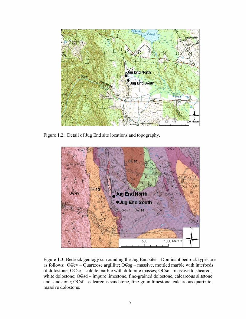
Figure ................................................... Page 1.1. Field site geographic locations with watershed and sub-drainage basin boundaries ............................................................................................................... 6 1.2. Detail of Jug End site locations and topography ........................................................ 8

1.3. Bedrock geology surrounding the Jug End sites. Dominant bedrock types are as follows: OCev – Quartzose argillite; OCsg – massive, mottled marble with interbeds of dolostone; OCse – calcite marble with dolomite masses; OCsc – massive to sheared, white dolostone; OCsd – impure limestone, fine-grained dolostone, calcareous siltstone and sandstone; OCsf – calcareous sandstone, fine-grain limestone, calcareous quartzite, massive dolostone ................................................................................................................. 8

1.4. Detail of Schenob Brook site locations and topography ............................................. 10 1.5. Bedrock geology surrounding the Schenob Brook sites. Dominant bedrock

types are as follows: Ow – Schist or phyllite, locally calcareous, micaceous or quartzose; OCsf – calcareous sandstone, fine-grain limestone, calcareous quartzite, massive dolostone; OCsd – impure limestone, fine-grained dolostone, calcareous siltstone and sandstone; OCsc – massive to sheared, white dolostone; OCsb – uniform, massive dolostone; Qcd – water-laid ice-contact deposits; Qo – outwash ........................... 10

1.6. Detail of Shmulsky site locations and topography ..................................................... 12 1.7. Bedrock geology surrounding the Shmulsky sites. Dominant bedrock types

are as follows: Owm – Schistose marble mottled by phyllitic masses; Ow – Schist or phyllite, locally calcareous, micaceous or quartzose; OCsg – massive, mottled marble with interbeds of dolostone; OCsf – calcareous sandstone, fine-grain limestone, calcareous quartzite, massive dolostone; OCsc – massive to sheared, white dolostone; OCsb – uniform, massive dolostone; Qcd – water-laid ice-contact deposits; Qo – outwash ........................... 12

3.1. Water table depth (cm) at geographic location, a) Jug End, b) Schenob

Brook, c) Shmulsky from April 30, 2006 to October 18, 2006. Each point represents a mean of three replicate measurements ................................................ 31

3.2. Vertical groundwater gradients at locations a) Jug End, b) Schenob Brook, c)

Shmulsky. Values greater than zero represent discharge conditions; values less than zero represent recharge conditions. Each bar represents one pair of piezometers at a central location in each site ..................................................... 34

xix

Figure ................................................... Page 3.3. a. Seasonal variation in water calcium (mg.L-1) at the Jug End location.

Each point represents a mean of three replicate samples. b. A comparison with seasonal water table depth .............................................................................. 37

3.4. a. Seasonal variation in water calcium (mg.L-1) at the Schenob location.


3.5. a. Seasonal variation in water calcium (mg.L-1) at the Shmulsky location.


3.6. Seasonal variation in water magnesium (mg.L-1) at a) Jug End, b) Schenob

Brook and c) Shmulsky. Each point represents a mean of three replicate samples .................................................................................................................... 42

3.7. Seasonal variation in calcium to magnesium ratios for the eight study sites.

Each point represents a mean of three replicate samples ........................................ 45 3.8. Seasonal variation in water iron (mg.L-1) at the a) Jug End, b) Schenob Brook

and c) Shmulsky locations. Each point represents a mean of three replicate samples ..................................................................................................... 47

4.1. The relationship between soil N:P (log of ratio of total nitrogen to AB-DTPA extractable phosphorus) and species richness at the 24 study plots. ....................... 75 5.1. Two-dimensional (Axis 1 and Axis 3) ordination of study plots represented

in species space. r2= 0.293 for all variables shown (Axis1: r2=0.123, Axis3: r2=0.170). Larger distances between plots represent greater dissimilarity in species composition at those plots. Symbols are coded by location (shapes), and site (colors). Refer to legend in Figure 4.1 for full clarification ............................................................................................................. 82

5.2. Joint plot of species with linear correlations (r2 > 0.4) to species space (see Table 5.1). Symbols are coded by location (shapes), and site (colors). Refer to legend in Figure 5.1 for full clarification .................................................. 84 5.3. Joint plot of environmental variables with linear correlations (r2 > 0.2) to

species space (see Table 5.2). Symbols are coded by location (shapes), and site (colors) (see Figure 5.1) ............................................................................. 86

xx

Figure ................................................... Page 5.4. Three-dimensional ordination of study plots represented in environmental

space. a) Axis 1: r2=0.531 and Axis 2: r2= 0.141, b) Axis 1: r2=0.531 and Axis 3: r2= 0.120. Cumulative r2=0.792. Larger distances between plots represent greater dissimilarity in species composition at those plots. Symbols are coded by location (shapes), and site (colors). Refer to legend in Figure 4.1 ............................................................................................................ 90

5.5. Joint plot of environmental properties with linear correlations (r2 > 0.4) to

environmental space on a) Axis 1 and Axis 2 and b) Axis 1 and Axis 3 (see Table 5.3). Symbols are coded by location (shapes), and site (colors). Refer to legend in Figure 5.4 .................................................................................. 93

5.6. Joint plot of species with linear correlations (r2 > 0.2) to environmental space

on a) Axis 1 and Axis 2 and b) Axis 1 and Axis 3 (see Table 5.4). Symbols are coded by location (shapes), and site (colors). Refer to legend in Figure 5.4 ............................................................................................................ 96

5.7. PC-ORD output representing the linear correlation between Axes 2 and 3 and mean water calcium .......................................................................................... 102 5.8. PC-ORD output for the overlay of the distribution of a) Carex granularis, b)

Carex sterilis, and c) Geum rivale along the axes (2 and 3) where water calcium is the strongest explanatory variable ......................................................... 103

5.9. Abundance of Carex granularis as compared to mean water calcium.

Statistics are based on log-transformed data; raw data are presented in the graph. Each point represents a mean for that site (n=3) ........................................ 104

5.10. Abundance of Carex sterilis as compared to mean water calcium. Statistics

are based on log-transformed data; raw data are presented in the graph. Each point represents a mean for that site (n=3)..................................................... 105

5.11. Abundance of Geum rivale as compared to mean water calcium. Statistics

are based on square root-transformed data; raw data are presented in the graph. Each point represents a mean for that site (n=3). NS = not significant ................................................................................................................ 105

5.12. PC-ORD output for the overlay of the distribution a) Parnassia glauca, b)

Carex leptalea along the axes (2 and 3) where water calcium is the strongest explanatory variable. This distribution indicates that these species increases in abundance as calcium levels increase and are thus considered gradient species ..................................................................................... 107

xxi

Figure ................................................... Page 5.13. PC-ORD output for the overlay of the distribution of Juncus

brachycephalus along Axis 1, where water pH is a strong explanatory variable .................................................................................................................... 108

5.14. Abundance of Equisetum fluviatile as compared to minimum water iron.

Statistics represent log-transformed data, raw data are presented. Each point represents a mean for that site (n=3) ............................................................. 109

5.15. Abundance of Parnassia glauca as compared to mean water calcium. Raw data are presented. Each point represents a mean for that site (n=3) ..................... 109 5.16. Abundance of Packera aurea as compared to mean water calcium. Raw

data are presented. Each point represents a mean for that site (n=3). No significant relationship occurred between abundance and calcium concentrations in water ........................................................................................... 110

5.17. Abundance of Thelypteris palustris as compared to mean water calcium.

Raw data are presented. Each point represents a mean for that site (n=3). No significant relationship occurred between abundance and mean concentrations of calcium in water ......................................................................... 110

5.18. Abundance of Carex leptalea as compared to mean water calcium. Raw

data are presented. Each point represents a mean for that site (n=3). No significant relationship occurred between abundance and mean concentrations of calcium in water ......................................................................... 111

5.19. Abundance of Dasiphora fruticosa as compared to mean water pH. Raw data are presented. Each point represents a mean for that site (n=3) ..................... 112 5.20. Abundance of Juncus brachycephalus as compared to mean water pH. Raw

data are presented. Each point represents a mean for that site (n=3). No significant relationship occurred between abundance and mean water pH ............ 112

6.1. Percent calcium in the tissues of Parnassia glauca as a function of mean

water calcium in June and soil calcium. Equations and statistics refer to the line that they are in closest proximity to ........................................................... 127

6.2. Best fit line (exponential rise, single, 2 parameter) for relationship between

percent calcium in the tissues of Parnassia glauca as a function of mean water calcium in June and soil calcium. Equations and statistics refer to the line that they are in closest proximity to ........................................................... 129

xxii

Figure ................................................... Page 6.3. Percent calcium in the tissues of Equisetum fluviatile as compared to mean


6.4. Percent calcium in the tissues of Symphyotrichum puniceum as compared to

mean water calcium in June and soil calcium. Equations and statistics refer to the line that they are in closest proximity to .............................................. 131

6.5. Percent calcium in the tissues of Packera aurea as compared to mean water

calcium in June and soil calcium. Equations and statistics refer to the line that they are in closest proximity to ........................................................................ 132

6.6. Percent calcium in the tissues of Symplocarpus foetidus as compared to mean


6.7. Percent magnesium in the tissues of Thelypteris palustris as compared to

mean water magnesium in June and soil magnesium. Equations and statistics refer to the line that they are in closest proximity to ................................ 138

6.8. Percent magnesium in the tissues of Carex flava as compared to mean water

magnesium in June and soil magnesium. Equations and statistics refer to the line that they are in closest proximity to ........................................................... 139

A.1. The Stockbridge Formation (Zen and Ratcliffe, 1971) .............................................. 154 B.1. Vegetation community at Jug End North ................................................................... 156 B.2. Vegetation community and water monitoring instruments at Jug End South ............ 157 B.3. General vegetation at of Schenob Brook Bartholomew: a) plot SBB3, b) adjacent agricultural fields ...................................................................................... 158 B.4. General view of vegetation at Schenob Brook North ................................................ 159 B.5. Unique species at Schenob Brook North: a) Pogonia ophioglossoides, b) Calopogon tuberosus, c) Spiranthes cernua ........................................................... 160 B.6. Vegetation community at Schenob Brook Central in autumn of 2006 ...................... 161

B.7. Hummock landscape at Schenob Brook South before the emergence of vegetation in March, 2006 ...................................................................................... 162

xxiii

Figure ................................................... Page B.8. Vegetation at Shmulsky Open: a) general fen view, and b) plant composition and sampling well at SO1 ....................................................................................... 163 B.9. Vegetation cover at Shmulsky Shrub, plot 1 .............................................................. 164 C.1. Reduced iron at Jug End North (JN) .......................................................................... 166

C.2. Reduced iron at Jug End South (JS) ........................................................................... 166

C.3. Reduced iron at Bartholomew (SBB) ......................................................................... 167

C.4. Reduced iron at Schenob Brook Central (SBC) ......................................................... 167

C.5. Reduced iron at Schenob Brook North (SBN) ........................................................... 168

C.6. Reduced iron at Schenob Brook South (SBS) ............................................................ 168

C.7. Reduced iron at Shmulsky Open (SO) ....................................................................... 169

C.8. Reduced iron at Shmulsky Shrub (SS) ....................................................................... 169

D.1. Seasonal variation in water pH at the two sites in the Shmulsky location ................. 171

D.2. Seasonal variation in water pH at the four sites in the Schenob Brook location .................................................................................................................... 171 D.3. Seasonal variation in water pH at the two sites in the Jug End location .................... 172

1

1

CHAPTER I

INTRODUCTION

The distribution and occurrence of plant species within a given community provides

insight into the many environmental properties of the climate to which that community is

exposed, (i.e., precipitation, temperature, humidity, wind, etc.) as well as to the soil

environment where it occurs (i.e. pH, available nutrients, water, disturbance, etc.). Plant

communities and individual species occurrences have been documented around the world

for hundreds of years, and especially in the last sixty years, numerous efforts have been

made to associate those occurrences with specific environmental properties. However,

the characteristics of individual plant species that either reflect or influence their

environmental habitat selections within those communities are less studied.

Calcareous fens are wetlands that harbor many rare plants and uncommon plant

communities, in addition to being core habitat for the federally threatened Bog Turtle

(Glyptemys muhlenbergii). These associations are due to the unique hydrogeochemical

environment caused by the upwelling of mineral-rich groundwater that has passed

through bedrock or parent material rich in calcium carbonate, relative to wetlands

underlain by other strata. The resulting root-zone contains elevated calcium levels and

elevated pH. Since these conditions, along with the limited occurrence of carbonate

bedrock in New England, are rare, so too are the associated plant communities. In

Massachusetts, calcareous fens harbor many uncommon plant species, six of which are

threatened or of special concern (MNHESP, 2004).

For many years, calcareous fens have been a topic of study for their unique chemical

properties, plant assemblages, rare fauna and overall ecological importance. These

2

studies have concluded that the unique vegetative assemblages and high occurrence of

rare and endangered species are attributable to the minerotrophic properties of the fen

wetlands, notably elevated pH and calcium concentrations (Sjörs, 1950; Vitt et al., 1975;

Slack et al., 1980; Vitt and Chee, 1990; Motzkin, 1994; Picking and Veneman, 2004).

However, no research has yet attempted to isolate the specific geochemical conditions

associated with individual species in the fens (Godwin et al., 2002). Certain calciphiles

are generalists in terms of calcium requirements, whereas others appear to occur only at

distinctly elevated calcium levels (Motzkin, 1994; Picking and Veneman, 2004). It is not

yet clear what threshold values are necessary for a given calciphile to occur. In addition,

no studies have yet attempted to document and compare the physiological response of

individual species in calcareous fens to elevated environmental calcium levels and how

this response may be associated with their distributions.

Justification

This research is an effort to determine environmental calcium requirements for rare as

well as common indicator species of calcareous fens in Massachusetts. In addition, it

seeks to examine the physiological relationship between these plant species and

environmental calcium availability by measuring the concentrations of calcium in their

tissues. The extent to which these plants selectively absorb calcium and how those levels

relate to levels of calcium in the substrate environment and to their overall distribution

patterns is also analyzed. Early on, several European researchers compared the

relationships between plant tissue calcium in species that preferred to grow on calcareous

soils to those that did not (Molisch, 1918; Iljin, 1936; Kinzel, 1963) and others have

measured nutrient accumulation in the tissues of wetland plants (Boyd and Hess, 1970;

3

Auclair, 1979). However, no studies have yet examined calcium accumulation in plant

species in calcareous fens.

Knowledge of the suspected calcium requirements of these species is important for

conservation efforts as it will allow for a means of identifying specific regions with

suitable substrates for these rare communities that then can be prioritized for preservation

or targeted for restoration. Understanding the specific limitations for these rare plant

species and communities may help to elucidate causes of population changes or local

disappearances, whether natural or anthropogenic. Although no definitive conclusions

can be made as to locations where plants are notably absent, trends in environmental

properties in these regions may provide clues as to the selectivity of the absent species.

There is also a need for a more comprehensive analysis of the geochemical properties

of some previously studied calcareous fens. Picking (2002) studied vegetation patterns in

a single calcareous sloping fen in Massachusetts by analyzing pore-water and soil

chemistry in the plant root-zone. Other researchers studying calcareous fens in North

America (Slack et al., 1980; Vitt and Chee, 1990; Motzkin, 1994) have measured surface

water chemistry that may not have been reflective of actual pore-water conditions due to

the unavoidable “degassing” of the CO2. This phenomena would have resulted in lower

calcium values and higher pH compared to measurements at below-surface depths (Schot

and Wassen, 1993). In addition, several researchers have measured the water chemistry

but neglected the chemistry of the soil (Vitt et al., 1975; Slack et al., 1980; Vitt and Chee,

1990; Motzkin, 1994; Godwin et al., 2002). Conversely, some have measured the soil

chemistry but neglected the water chemistry (Nekola, 2004; Bowles et al., 2005). To

analyze the soil environment from the perspective of a plant, it will be important to

4

monitor, as Picking did, the soil chemistry as an indicator of the reserve nutrient pool and

the pore-water chemistry (not surface water) to determine the readily available nutrients.

This study is the first of its kind to compare individual plant-tissue calcium levels to

substrate calcium levels in calcareous fens and to analyze this relationship in terms of the

distribution of plants in relation to substrate calcium. In this context, it is the first to

examine the water and soil chemical environments for multiple calcareous fens in

Massachusetts, including some fen systems that have not been studied previously.

Hypothesis

The hypothesis of this study is that calciphiles select habitats in calcareous fens that

have significantly elevated calcium levels and that this trend can be evidenced in how

those plants selectively absorb calcium into their tissues. Thus:

• Specific environmental substrate calcium levels can be measured, and for the

most selective species, a minimum threshold and maximum range can be

established.

• The most selective calciphile species (calcium specialists) that grow in calcareous

fens will have the highest calcium concentrations in their tissues, and these levels

will correspond to environmental substrate calcium levels.

• The least selective calciphiles (calcium generalists) will maintain lower tissue

calcium levels (than the specialists), and these levels are independent of

environmental substrate levels.

Objectives

1) A list of target species was compiled from previous literature reports of vegetation

in calcareous fens of Massachusetts. These species were grouped by their

5

suspected selectiveness to environmental calcium levels (generalists vs.

specialists).

2) Field locations were chosen where species from the compiled list naturally

occurred. Vegetation was surveyed in each study location, and plant tissues were

collected and analyzed for calcium accumulation for selected species.

3) Soil and soil-water samples were analyzed for calcium and other key element

concentrations and pH throughout the growing season to determine the nutritional

conditions to which the plants are exposed.

4) Hydrologic characteristics of the wetland systems were monitored throughout the

growing season and physical properties of the soils were described to be able to

identify when environmental properties other than substrate calcium levels may

be limiting or controlling plant distributions.

5) Suspected ranges and thresholds of substrate calcium were established for

selected species, and these data were compared to the levels of calcium in the

plant tissues.

Study Site Layout

Previous studies (Motzkin, 1994; Kearsley, 1999; Picking, 2002) in the Berkshire-

Taconic region of New York and Massachusetts have established that many of the

wetland communities occurring there are calcareous. The principal bedrock underlying

the surficial deposits are various forms of calcitic limestone (CaCO3) and dolomitic

limestone (CaMg(CO3)2), known as the Stockbridge Formation (Appendix A; Zen and

Hartshorn, 1966; Zen and Ratcliffe, 1971). The Nature Conservancy oversees many of

these properties and was contacted to help identify geographic locations known to contain

6

calcareous wetlands with the desired suite of plant species. Three geographic locations

were identified within the Housatonic Watershed (Figure 1.1). In March 2006, eight

research sites were established across the three geographic areas where calcareous

wetland conditions existed and vegetation was dominantly herbaceous, graminoid, or low

shrub cover. Different study sites within one geographic region were chosen by selecting

areas within the region where distinct differences were observed in the vegetative

Figure 1.1. Field site geographic locations with watershed and sub-drainage basin boundaries.

7

community and the hydrologic input, with sufficient area for sampling to occur in

triplicate. By mid-April 2006, three replicate plots were chosen in each of the selected

sites where data collection took place. The plots were set up approximately 10 m from

each other. Plots were arranged so that, when possible, they existed in a triangular

arrangement. In some instances the small size of the open fen area did not allow for this

arrangement, and thus plots were arranged so that they were linear and followed the

contour of the wetland hydrologic gradient.

Two study sites were established at location Jug End; four were established at location

Schenob Brook (including one at nearby Bartholomew); and two sites were established at

location Shmulsky (Figure 1.1). Photographs of sites are available in Appendix B.

Hydrogeochemical Setting

The Jug End geographic location (Figure 1.2) lies much farther north than the other

regions (which cluster around the Schenob Brook). It is surrounded by residential

structures to the north and west and agriculture to the south. A long, protected wetland

region lies to the east. This region occurs at the base of a hill where water seeps into the

lowland. The hill area contains 15-35% calcitic limestone outcrops and has low

permeability. The substratum of the fen complex is thin till and has some limestone

outcrops (Scanu, 1988). The hill area is comprised of calcitic marble with interbeds of

dolomitic limestone, and the bedrock underlying the fen complex is a mix of various

forms of calcitic and dolomitic limestone (Zen and Ratcliffe, 1971) (Figure 1.3). The Jug

End North site (JN), which lies in the northwestern portion of the fen, is situated at the

location where water seeps out from the hill. The other site, Jug End South (JS), lies in

the southwestern region of the fen.

8

Figure 1.2: Detail of Jug End site locations and topography.

Figure 1.3: Bedrock geology surrounding the Jug End sites. Dominant bedrock types are as follows: OCev – Quartzose argillite; OCsg – massive, mottled marble with interbeds of dolostone; OCse – calcite marble with dolomite masses; OCsc – massive to sheared, white dolostone; OCsd – impure limestone, fine-grained dolostone, calcareous siltstone and sandstone; OCsf – calcareous sandstone, fine-grain limestone, calcareous quartzite, massive dolostone.

9

9

The Schenob Brook geographic location (Figure 1.4) is just north of the confluence of

the smaller Dry Brook and Schenob Brook. Two of the sites, Schenob Brook Central

(SBC) and Schenob Brook North (SBN), occur where a long kame terrace slopes steeply

to meet with water-sorted outwash deposits (Zen and Hartshorn, 1966) in a lowland area.

At this location, water flows directly from these deposits and into the lowland, creating

the wetland fen areas and forming rivulets that separate the vegetation-bearing

hummocks. This feature is particularly pronounced at Schenob Brook Central, were the

rivulets are comprised of flowing water from the seep areas. The substrates of these two

sites are gravelly to sandy glacio-fluvial materials derived from slate, shale, sandstone,

limestone, and small amounts of granitic gneiss (Scanu, 1988). These two sites are

bordered by the protected fen complex to the south and east and are bordered by open

fields and few residential structures to the north and west. The third site, Schenob Brook

South (SBS), occurs in a similar landscape position as the other Schenob sites but

somewhat closer toward the Dry Brook-Schenob Brook floodplain region. Thus, the

substratum is comprised of silty alluvial deposits. This site is surrounded immediately by

forest and wetland, but like the other Schenob Brook sites, it has the same agricultural

and residential land use 50 m to the west. The principal bedrock surrounding these three

Schenob Brook sites is chiefly calcareous in nature, mostly that of dolomitic limestone

(Figure 1.5; Zen and Hartshorn, 1966). However, on the ridge areas, the bedrock is

comprised of schist or phyllite with small calcareous pockets.

The Bartholomew site (SBB) lies in the Schenob Brook geographic location (Figure

1.4) and is near the Dry Brook, farther downstream from the other Schenob Brook sites.

The geomorphology is similar to the Schenob sites (situated at the base of a kame terrace

10

10

Figure 1.4: Detail of Schenob Brook site locations and topography.

Figure 1.5: Bedrock geology surrounding the Schenob Brook sites. Dominant bedrock types are as follows: Ow – Schist or phyllite, locally calcareous, micaceous or quartzose; OCsf – calcareous sandstone, fine-grain limestone, calcareous quartzite, massive dolostone; OCsd – impure limestone, fine-grained dolostone, calcareous siltstone and sandstone; OCsc – massive to sheared, white dolostone; OCsb – uniform, massive dolostone; Qcd – water-laid ice-contact deposits; Qo – outwash.

11

11

where water seeps into outwash deposits; Figure 1.5), but the substratum is formed from

calcareous, loamy till and contains 10 to 35 percent coarse fragments (Scanu, 1988). As

were the Schenob sites, Bartholomew is surrounded by dolomitic limestone (Figure 1.5;

Zen and Hartshorn, 1966); however, it is situated much more closely to a pocket of

calcitic marble and limestone. The site is bordered to the east by forest and floodplain

wetlands and to the west by fields used for vegetable production.

The Shmulsky geographic region (Figure 1.6) occurs several miles downstream and

northeast of the Schenob Brook geographic location, draining into a lower reach of the

Schenob Brook watershed. Sandy glacio-fluvial deposits form the substratum (Scanu,

1988) in this lowland region that occurs slightly up gradient from the brook and down

gradient from a bedrock of schistose marble from the Walloomsac formation and

calcareous sandstone, and calcitic and dolomitic limestone from the Stockbridge

formation (Figure 1.7; Zen and Hartshorn, 1966). The region is surrounded mainly by

wet meadows, forest, and a few residential structures. The site Shmulsky Open (SO) is

an open, graminoid-herbaceous fen meadow. The other site, Shmulsky Shrub (SS), is

about 100 m north of SO and is characterized by low shrub cover in combination with

graminoid and herbaceous vegetation.

12

12

Figure 1.6: Detail of Shmulsky site locations and topography.

Figure 1.7: Bedrock geology surrounding the Shmulsky sites. Dominant bedrock types are as follows: Owm – Schistose marble mottled by phyllitic masses; Ow – Schist or phyllite, locally calcareous, micaceous or quartzose; OCsg – massive, mottled marble with interbeds of dolostone; OCsf – calcareous sandstone, fine-grain limestone, calcareous quartzite, massive dolostone; OCsc – massive to sheared, white dolostone; OCsb – uniform, massive dolostone; Qcd – water-laid ice-contact deposits; Qo – outwash.

13

CHAPTER II

LITERATURE REVIEW

Wetland Hydrology

A wetland is defined as a natural landscape characterized by saturated surface soil

and/or shallow standing water, in which unique soil morphological features develop

(gleization and organic matter accumulation) and where the vegetation is specifically

adapted to such conditions (Mitsch and Gosselink, 1993). Although all wetlands share

these characteristics, great variability exists in the mechanisms that cause water to

accumulate. At least sixteen different terms have been used to describe the many

differences among wetlands; most commonly used are swamp, marsh, bog, and fen.

Marshes are often continually inundated areas with emergent vegetation; bogs have no

significant inflow and are primarily rain fed; and swamps often are forested regions

produced by overflowing streams in low-lying areas or perched water tables (Mitsch and

Gosselink, 1993). All of these wetlands are characterized by receiving water from the

surface. By contrast, a fen is a wetland that receives water from underground sources

that originate in the underlying parent materials or bedrock (Bedford and Godwin, 2003).

Although these wetland titles at times are used interchangeably, a fen is distinctly

different in that it is a groundwater fed system.

Fens are “discharge” wetlands, indicating that the hydraulic head in the wetland is

lower than the hydraulic head underlying the surrounding landscape. Fen wetlands often

result where groundwater inflow forms a spring or seep at the base of a steep slope or

where pressurized groundwater has an outlet to the surface (artesian conditions; Brooks et

al., 1997). By contrast “recharge” wetlands like bogs, swamps, and marshes have a

14

downward hydrologic gradient that recharges the groundwater (Mitsch and Gosselink,

1993).

Fen Geochemistry

On average, the pH of wetland soils and waters tends to range from acidic to neutral as

they lack a constant supply of base cations from groundwater inputs. This condition,

combined with the nature of the vegetation in the wetland (and thus the level of

production of organic acids) maintains the pH of most wetlands between 3.5 and 6.5.

Bogs are often on the lower end of this range due to organic acid production from

sphagnum mosses (Sphagnum spp.) (Mitsch and Gosselink, 1993).

Non-fen wetland systems are called ombrotrophic (ombro meaning “rain” and trophic

meaning “nourishment”) as they rely on precipitation or surface water for their sparse

supply of nutrients. The resulting water chemistry reflects in situ chemical processes and

rain water characteristics, not the geochemistry of the watershed. However, fens are

called minerotrophic (Vitt and Chee, 1990) in that their water chemistry is related directly

to the local bedrock and parent material. Fen pH may range from 3.5 (similar to bog

environments) to 8.4 (Bedford and Godwin, 2003) depending on the mineralogy of the

substratum surrounding it.

In an attempt to qualify the differences in fen pH, terminology has been developed to

classify these characteristics. An acidic fen (pH 3.5-5.5) is called a “poor fen”; a

circumneutral fen (pH 5.5-7.4) is called a “rich fen”; and when a fen is strongly alkaline

(pH 7.5-8.4) it is called an “extreme rich fen” or a “marl fen” (Bedford and Godwin,

2003). One type of rich fen called a “calcareous fen” occurs when the hydrologic input

for the fen is supplied by water that has traveled through calcareous bedrock such as

15

calcitic and dolomitic limestone, or metamorphosed forms of either of the two. Many

studies have established the water pH range in calcareous fens to be between 6.0 and 8.1

(Slack et al., 1980; Komor, 1994; Motzkin, 1994; Picking and Veneman, 2004), and that

fens are characterized as having unusually high levels of dissolved calcium in the water

and adsorbed to the soil.

Vitt et al. (1975) concluded that dissolved calcium values greater than 5 mg.L-1 were

characteristic of rich fens; however, other studies have reported higher threshold values.

Slack et al. (1980) reported dissolved calcium to range from 18 to 37 mg.L-1, whereas

Motzkin’s (1994) rich fen values approached 65 mg.L-1. The highest values were

detected by Komor (1994) who measured values up to 128 mg.L-1 and by Picking (2002)

who reported comparable water calcium values approaching 180 mg.L-1 and soil calcium

values ranging from 2126 g.m-3 to 4907 g.m-3.

Calcareous bedrock has a limited distribution in the United States (National Atlas,

2006). It has scattered occurrences in the western United States with most notable areas

in northwestern Arizona, south-central New Mexico, and central Texas. In the Upper

Midwest it occurs significantly in Iowa, Missouri, and Wisconsin and moderately in

Michigan, Indiana, Illinois, and Ohio. Although abundant in Florida and southern

Georgia, it has scattered occurrences in the southeastern states of Kentucky and

Tennessee. In the Mid-Atlantic and New England, it only occurs in thin bands. For this

reason, calcareous fens occur infrequently and exist only as small communities,

especially in Massachusetts.

16

Fen Plant Communities

Eggers and Reed (1987) referred to plant communities associated with calcareous fens

as the rarest in North America. As may be expected, many of the plant species that occur

in these habitats are adapted specifically to the unique geochemical conditions present,

and thus the plant assemblages are unique and often harbor many rare and endangered

species. Bowles et al. (2005) reported that the vegetative communities in a 23-hectare

prairie fen in Illinois were correlated significantly with soil pH, sodium, magnesium, and

calcium concentrations. Motzkin (1994), in a study of western New England fens,

established species groupings that have been since used and validated by other

researchers (Kearsley, 1999; Picking and Veneman, 2004) to describe the vegetation.

These species groupings were related to differences in environmental properties, with

depth to the mineral soil being the most important, but also important were pH,

magnesium, and calcium in the fen waters. Vitt and Chee (1990) showed a strong

correlation between vegetative communities and fen pH, calcium, magnesium, and

electrical conductivity in their study of water and peat chemistry of fens in Alberta,

Canada. They identified distinctly different species associations between the extreme-

rich fens, moderate-rich fens, and poor fens. In addition, vegetation assemblages were

further separated by other hydrologic and geomorphologic aspects of the fens. For

example, a “calcareous seep” community occurs where calcareous groundwater seeps off

of a slope to the soil surface forming rivulets. A “lake-basin” fen community occurs

where calcareous groundwater travels through peat that has accumulated in a former lake

basin (most likely of glacial origin; Weatherbee, 1996).

17

The previous studies documented that calcareous fens have high species richness, as

do many places with rare and uncommon species. Species richness has often been

explained in terms of nutrient availability in wetlands. Bowden (1987) reported that most

freshwater wetlands are limited by nitrogen. However, several other researchers

(Richardson and Marshall, 1986; Boyer and Wheeler, 1989) proposed that phosphorus is

limited under conditions with elevated levels of calcium or aluminum (as these elements

bind phosphorus in insoluble forms). In agreement, Bedford et al. (1999) reported that

wetlands in North America often are limited by low levels of phosphorus or by a

combination of low levels of nitrogen and phosphorus (two of the primary macronutrients

required by plants). Bedford et al. (1999) reported that bogs and fens had high total N:P

ratios (>16) that were indicative of phosphorus limitation and that swamps and marshes

had lower total N:P ratios (<14) indicative of nitrogen as the limiting nutrient. They

reported that higher N:P ratios were associated with higher species richness and percent

organic matter in the surface soil. Plants that thrive under nutrient enriched conditions

are often larger in size and more vigorous in growth than those that require fewer

nutrients (Reader, 1990). Thus when conditions are more eutrophic, the nutrient-loving

species tend to dominate and species richness is lower.

Calcium in Plants

Calcium is considered a secondary macronutrient for plant survival. The fundamental

role of calcium in plants is in the strengthening of the cell walls as calcium pectates,

although calcium is also vital in cell nuclear division by providing elasticity to

microfibers, stabilizing plant membranes by bridging phosphate and carboxylate groups

in phospholipids and proteins (Marschner, 1995), and providing a counter-cation for

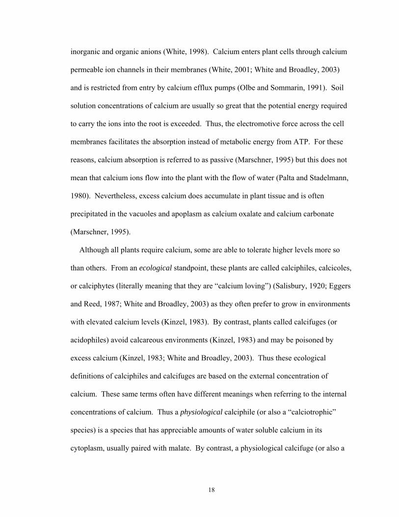
18

inorganic and organic anions (White, 1998). Calcium enters plant cells through calcium

permeable ion channels in their membranes (White, 2001; White and Broadley, 2003)

and is restricted from entry by calcium efflux pumps (Olbe and Sommarin, 1991). Soil

solution concentrations of calcium are usually so great that the potential energy required

to carry the ions into the root is exceeded. Thus, the electromotive force across the cell

membranes facilitates the absorption instead of metabolic energy from ATP. For these

reasons, calcium absorption is referred to as passive (Marschner, 1995) but this does not

mean that calcium ions flow into the plant with the flow of water (Palta and Stadelmann,

1980). Nevertheless, excess calcium does accumulate in plant tissue and is often

precipitated in the vacuoles and apoplasm as calcium oxalate and calcium carbonate

(Marschner, 1995).

Although all plants require calcium, some are able to tolerate higher levels more so

than others. From an ecological standpoint, these plants are called calciphiles, calcicoles,

or calciphytes (literally meaning that they are “calcium loving”) (Salisbury, 1920; Eggers

and Reed, 1987; White and Broadley, 2003) as they often prefer to grow in environments

with elevated calcium levels (Kinzel, 1983). By contrast, plants called calcifuges (or

acidophiles) avoid calcareous environments (Kinzel, 1983) and may be poisoned by

excess calcium (Kinzel, 1983; White and Broadley, 2003). Thus these ecological

definitions of calciphiles and calcifuges are based on the external concentration of

calcium. These same terms often have different meanings when referring to the internal

concentrations of calcium. Thus a physiological calciphile (or also a “calciotrophic”

species) is a species that has appreciable amounts of water soluble calcium in its

cytoplasm, usually paired with malate. By contrast, a physiological calcifuge (or also a

19

“calciophobic” species) is a species that contains high amounts of oxalate, which

facilitates the precipitation of calcium that enters (Kinzel, 1983).

Both physiotypes occur on calcareous soils. True calciotrophic species (physiological

calciphiles) are less common as wild plants in North America (compared to the

calciophobic species) since they mostly occur in the Crassulaceae, Brassicaeae, and

Fabaceae families. Many of the calciphiles that are also calciophobic have a greater

capacity to store calcium due to elevated levels of calcium-binding proteins in their

cytoplasm (Le Gales et al., 1980). This ability may make them better competitors under

calcareous conditions and thus receive the “calciphile” designation. By contrast, calcium

toxicity is often a result of a plants’ inability to compartmentalize the calcium or

inactivate it physiologically (i.e. producing calcium oxalate, calcium carbonate, etc.)

(Marschner, 1995) and this may result in the habitat selections of calcifuges.

Early research on calcium in plants reported that excess calcium had no toxic effect

and that toxicity symptoms were due to increased levels of associated anions e.g., Cl- and

NO3- (Gauch, 1972). However, more recent studies have concluded that excess calcium

in the cytoplasm does prevent stomatal opening (Atkinson, 1991; Ruiz et al., 1993),

photosynthetic ability (Portis et al., 1977), and water-use efficiency (Da Silva et al.,

1994). Detrimental levels of calcium may exist within a plant if its adaptations to

calcium absorption are more efficient in a non-calcareous habitat. For example, if a

plants’ absorption of calcium is adapted to calcium-poor conditions (such as is a

calcifuge) it may have an overexpression of calcium transporters that act to maximize

calcium absorption. When attempting to grow under extremely elevated calcium

conditions, it consequently accumulates more calcium than it can effectively tolerate. By

20

contrast, calciphiles are believed to have adaptations that allow them to minimize calcium

influx and maximize calcium efflux. When attempting to grow under lower calcium

levels however, those calcium restrictive mechanisms are too efficient and do not allow

enough calcium for normal growth (Lee, 1999; White and Broadley, 2003).

Fen Plant Nutrition

Although calcium and magnesium are certainly not limited in calcareous fens, the

elevated pH of these systems affects the availability of other compounds and plant

nutrients. Specifically, when pH is above 7, bicarbonate is elevated, and the availabilities

of iron, phosphate, cobalt, and boron are limited. In addition, elevated amounts of

divalent cations (i.e. calcium and magnesium ions) may inhibit the ability for plants to

absorb potassium (Ehrenberg, 1919; Lee, 1999). Thus, researchers suspect that it may be

the ability to tolerate these nutrient limitations, rather than the potential benefits or toxic

effects of excess calcium that ultimately result in the calciphile/calcifuge habitat

distinction (Kinzel, 1983). For example, studies have shown that calciphiles have special

adaptations that allow them to increase absorption of iron by 1) having the ability to

promote the reduction of ferric iron to ferrous iron, 2) lower the pH around their roots, or

3) produce chelating agents (Römheld, 1987). Calciphiles also exude low-molecular

weight organic acids that act as extractors of iron and phosphate (Tyler and Ström, 1995).

By contrast, calcifuge species have been shown to be poisoned by bicarbonate as it

inhibits the uptake of iron into the plants (Woolhouse, 1966).

Calcium Uptake

A typical angiosperm contains between 0.1% and 5% calcium on a dry weight basis

(Marschner, 1995) but certain species of algae have as high as 11% (Boyd, 1966). Dicots

21

generally have higher tissue calcium than monocots (Loneragan et al., 1968). This

difference has been attributed to higher cation exchange capacity (CEC) of the roots of

dicots (Broadley et al., 2003) and to the fact that dicots have a lower ability to regulate

the passive influx of calcium ions (Kinzel, 1983). The accumulation of calcium in plant

leaves is based on the amount of absorption of calcium by the roots and its upward

translocation through the xylem. The rates of these processes are affected by the

availability of calcium, transpiration rates (Kinzel, 1983), and by the CEC of the roots

(Broadley et al., 2003), in which higher root CEC provides increased concentrations of

calcium at the root surface (Thompson et al., 1997).

Auclair (1979) measured the macro- and micronutrient tissue concentrations of six

species occurring in an emergent marsh and compared them to the soil nutrient

concentrations. Auclair reported that calcium concentrations in the six emergent wetland

plants varied between 0.27% and 1.8%. This study imparted important knowledge of

nutrient absorption in wetland plants, but since only one marsh habitat was studied,

inference of how these plants would accumulate nutrients in different geochemical

environments is unknown. Boyd and Hess (1970) showed that the calcium percentage in

cattail (Typha latifolia L.) varied from 0.35% to 1.62% across nineteen study sites.

These results indicate that there is variability in how much calcium a single species

accumulates, yet no comparisons of plant accumulation were made to environmental

calcium levels to understand if cattail regulates the amount of calcium it absorbs when

environmental levels differ.

In a laboratory experiment, Clarkson (1965) found that certain calciphile and calcifuge

species of bent-grass (Agrostis spp. L.) had equal accumulations of calcium in their

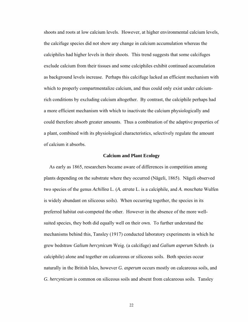
22

shoots and roots at low calcium levels. However, at higher environmental calcium levels,

the calcifuge species did not show any change in calcium accumulation whereas the

calciphiles had higher levels in their shoots. This trend suggests that some calcifuges

exclude calcium from their tissues and some calciphiles exhibit continued accumulation

as background levels increase. Perhaps this calcifuge lacked an efficient mechanism with

which to properly compartmentalize calcium, and thus could only exist under calcium-

rich conditions by excluding calcium altogether. By contrast, the calciphile perhaps had

a more efficient mechanism with which to inactivate the calcium physiologically and

could therefore absorb greater amounts. Thus a combination of the adaptive properties of

a plant, combined with its physiological characteristics, selectively regulate the amount

of calcium it absorbs.

Calcium and Plant Ecology

As early as 1865, researchers became aware of differences in competition among

plants depending on the substrate where they occurred (Nägeli, 1865). Nägeli observed

two species of the genus Achillea L. (A. atrata L. is a calciphile, and A. moschata Wulfen

is widely abundant on siliceous soils). When occurring together, the species in its

preferred habitat out-competed the other. However in the absence of the more well-

suited species, they both did equally well on their own. To further understand the

mechanisms behind this, Tansley (1917) conducted laboratory experiments in which he

grew bedstraw Galium hercynicum Weig. (a calcifuge) and Galium asperum Schreb. (a

calciphile) alone and together on calcareous or siliceous soils. Both species occur

naturally in the British Isles, however G. asperum occurs mostly on calcareous soils, and

G. hercynicum is common on siliceous soils and absent from calcareous soils. Tansley

23

noted that when grown on calcareous soils, many of the calcifuge seedlings that

germinated soon became chlorotic and died whereas the calciphiles exhibited normal

growth. The shoots of the calciphiles soon suppressed the growth of the few surviving

calcifuges. The reverse was true of the calciphiles on an acid substrate. Although it was

not determined why these plants responded as they did, Tansley concluded that calcifuges

are largely absent from calcium-enriched soils, not entirely because they are poisoned by

the calcium, but because the calciphiles are much better competitors under those

circumstances.

Subsequent researchers (Hope-Simpson, 1938; Rorison, 1960) later modified

Tansley’s findings, suggesting that soil chemistry was the primary factor governing the

abundance and growth of calciphiles and calcifuges, but that competition was of some

importance. Thus, calciphiles occupy a certain niche that is a combination of their

tolerance to potential geochemical toxicities and limitations and their competitive ability

under those conditions.

Habitat Conservation

The unique properties of calcareous fens have resulted in their receiving much

attention from scientists and conservationists. As a result, many of the properties on

which they occur are owned by various government and conservation organizations such

as The Nature Conservancy. The mission of The Nature Conservancy is “to preserve the

plants, animals and natural communities that represent the diversity of life on Earth by

protecting the lands and waters they need to survive” (www.nature.org). Active projects

associated with fen conservation from the Berkshire-Taconic chapter of The Nature

Conservancy have involved the management of non-native and invasive plants as well as

24

the application of prescribed burns. Purple loosestrife (Lythrum salicaria L.), and

common reed (Phragmites australis Trin. ex Steud.) are two common species considered

invasive in calcareous wetlands. They are given this title as they are often able to

outcompete the native species since they are not indigenous to the area and thus have

fewer adaptive pressures that limit their growth. Some varieties of common reed are

indigenous but inbreeding with more vigorous European varieties has resulted in the

current invasive nature of this species (Saltonstall, 2002). Without proper removal and

treatment, opportunities for the rare native plants will be limited.

Although not fully understood, it has been suspected that recurring fire has been a

major component in keeping calcareous wetlands open instead of eventually growing into

forested wetlands. Although some fen communities have had similar vegetation for

several thousand years, pollen records indicate that the open graminoid fen vegetation of

the Schenob Brook location has only been quite similar to the present since European

settlers arrived in the area 300 years ago (Shaw, 2003). The suppression of natural forest

fires by humans may pose a threat to some of these plant communities and thus The

Nature Conservancy is making every effort to recreate post-European settlement

conditions.

Although the aforementioned efforts are being made to protect these rare communities,

still more difficult challenges face conservationists. Studies have documented significant

changes in vegetation of naturally acidic Atlantic white cedar (Chamaecyparis thyoides

BSP.) swamps when they were subjected to nutrient loading from agriculture and

development (Ehrenfeld and Schneider, 1993; Zampella and Laidig, 1997). A similar,

opposite trend may be true for calcareous wetlands due to acidic inputs such as acid rain.

25

Studies of calcareous fens in the Netherlands have shown human usage of groundwater to

be a factor in reducing calcium levels in the wetlands (Grootjans et al., 1988). These

studies demonstrate the fragile geochemical makeup of a wetland community and show

that wetlands may be influenced by many outside sources. Determining suitable calcium

ranges for individual calciphiles will be essential to understanding precise changes in

plant communities due to associated changes in wetland hydrogeochemistry and may aid

in restoration efforts (e.g. returning peat mined fens to their original state) where a

knowledge of the precise geochemical conditions that native fen species require is

essential (Cobbaert et al, 2004).

26

CHAPTER III

HYDROLOGY, GEOCHEMISTRY, AND SOILS

Introduction

Calcareous fens are mineral-rich wetlands created by the upwelling of groundwater

through carbonate bedrock. Their occurrences are limited through a combination of

spatial factors. They must lie in an area where landscape features cause groundwater to

move to the surface and where that groundwater moves first through carbonate bedrock

to become enriched with dissolved carbonate minerals. Due to these unique conditions,

the geochemical properties of these wetlands are also unique, resulting in elevated

calcium and pH in the pore waters and soils. Due to the rare occurrence of these

conditions, especially in the northeastern United States were carbonate bedrock is quite

limited, these wetlands provide interesting study points for understanding bedrock

geochemistry as a determinant in the ion composition of surface soils.

This portion of the thesis study evaluated the hydrologic factors that exist in

calcareous fens and documented the level of calcium enrichment and pH that occurred in

eight study sites across the three geographic locations. The hydrology and geochemistry

were compared to examine the relationship between the two. Dissolved primary

macronutrients (nitrogen, phosphorus, potassium), iron, and magnesium also were

measured to provide a comprehensive understanding of the broad chemical environment

and to evaluate whether calcium was the primary defining element in site geochemistry

differences. Together, these factors help to further the understanding of the unique

geochemical properties in these wetlands and the plant communities that exist there.

27

Materials and Methods

Hydrologic Measurements

Instrument stations were installed in triplicate plots at each of the eight sites (spread

across the three geographic locations) and were installed directly up-gradient from where

vegetation was sampled later in the season. Each site was provided with a set of nested

piezometers (at depths of 100 cm and 150 cm or as far down as was possible given

substrate conditions) installed in a central location to measure the overall vertical

groundwater gradients at each site. Each sample plot included a 5-cm diameter PVC well

(screened from 0-60 cm) to measure groundwater level fluctuation and a suction

lysimeter (Soil Moisture Corporation, Goleta, Ca.; 0.1 MPa air entry value) at a depth of

30 cm to collect pore water.

According to the United States Natural Resources Conservation Service, the maximum

frost-free growing season for Great Barrington, Mass., is from April 10 to October 23

(NRCS, 2003). Due to accessibility restrictions posed by The Nature Conservancy

(related to critical breeding periods for bog turtles that live there), monitoring began in

late-April 2006 for half of the sites and did not begin until the beginning of June for the

others where conditions were more critical. Instruments were monitored biweekly until

October 18, 2006. A qualitative assessment of soil redoxomorphic conditions was

conducted at each visit using α, α-dipyridyl to identify the presence of reduced iron in

2.5-cm soil cores extracted from the top 0 to 15 cm and 15 to 30 cm, respectively.

Water Chemical Analysis

Twice monthly, after removing any passively accumulated water from the device,

fresh pore water samples were collected from the lysimeters. A vacuum was applied

28

using a hand pump, and lysimeters were allowed to fill for 2 to 3 hours before collection.

Water samples were siphoned from the lysimeters and were placed in acid-washed

polyethylene bottles, which were allowed to overflow before capping to minimize any

degassing of the samples. Samples were refrigerated for transport back to the laboratory

where the pH was measured immediately with a Hach EC-10 portable pH meter followed

by nutrient measurements. The general methodology of all water analyses is based on

standard methods detailed by Clesceri et al. (1989). One sample each month was

analyzed for orthophosphate (as a measure of phosphorus) by the Ascorbic Acid method

(4500-P.E); ammonium by Nessler’s method (4500-NH3.C); and total iron by the

Ferrover method (3500-Fe.D). These three analyses were carried out with prepackaged

reagents produced by The Hach Company (Loveland, Co., 1992) and analyzed using a

Hach DR/2000 Model Spectrophotometer (Hach, 1998). Studies have shown nitrate to be

almost non-detectable due to the anoxic nature of these systems (Picking, 2002) and for

this reason ammonium was the nitrogen species analyzed.

After these first analyses were finished, samples were acidified (with 1μL 1.0 M

HNO3 to prevent microbial growth) for refrigerated storage and later analyzed for

calcium (3500-Ca.B), magnesium (3500-Mg.B) and potassium (3500-K.B) by atomic

absorption/emission spectrophotometry. All samples were analyzed for calcium and

magnesium, however potassium was only analyzed once a month. Lanthanum was added

as an ionic suppressant for the calcium and magnesium samples and likewise cesium was

added to samples analyzed for potassium.

29

Soil Analysis

Soil samples were collected at each plot during the vegetation survey period in July

2006. Soil profile descriptions were recorded with standard terminology (Soil Survey

Staff, 1993). Samples were collected from each major horizon to a depth of 60 cm. After

taken to the laboratory, samples were air-dried and passed through a 2-mm sieve.

Samples were characterized physically and chemically, including particle size analysis

(pipette method; Gee and Bauder, 1986), bulk density (core method; Blake and Hartge,

1986), percent organic matter (loss on ignition; Dean, 1974), pH (water method; McLean,

1986), and exchangeable calcium, magnesium, and potassium (ammonium acetate

method; Thomas, 1986). Extractable phosphorus and iron (ammonium bicarbonate

diethylene triamine pentaacetic acid, AB-DTPA method; Soltanpour and Schwab, 1977)

and total nitrogen (Dumas method; Bremner and Mulvaney, 1986) also were measured

for the uppermost horizons. Early research has determined that the Dumas method

overestimates the total nitrogen in organic soils as compared to the Kjeldhal method

(Dyck and McKibbin, 1935; Bremmer and Shaw, 1958; Stewart, et al., 1963). However,

this has now been attributed to incomplete digestion of the Kjeldhal method (Miller et al.,

2007). This fact, along with increased accuracy of elemental analyzers that carry out the

Dumas method (early studies were from the mid-twentieth century) have resulted in

Dumas being the preferred method of analyzing total nitrogen (Watson and Galliher,

2001), including samples with large amounts of organic nitrogen (Miller et al., 2007).

Data Analysis

Statistical analyses were not applied to hydrologic measurements as these were

monitored to be able to view trends in saturation and vertical groundwater gradients. A

30

repeated measures analysis was conducted with statistical software (SAS Version 9.1.3,

SAS Institute, 2004) to determine if significant seasonal differences existed among the

nutrients in the water depending on the month, month by location and month by site

nested within the location. The multivariate test statistic, Wilks’ Lambda, was reported

to indicate when differences existed. This analysis also included an analysis of variance

(ANOVA) to detect significant differences in the nutrients among the different locations

and sites. A multivariate analysis of variance (MANOVA) was used to see if there were

overall differences in soil properties among the sites and locations and to see if

significant differences existed among individual soil properties (exchangeable calcium,

organic matter, etc.) among sites and locations. Tukey’s Test was applied (to be

conservative) to separate differences where they existed, as shown by the ANOVA.

Results and Discussion

Hydrologic Measurements

Well Data

Water table depth measurements indicated that the water tables in each wetland site

varied little within each geographic location but varied greatly among geographic

locations. The water table at the sites observed in the Shmulsky (Figure 3.1c) location

and the Jug End (Figure 3.1a) location appeared to have seasonal differences in that the

water table dropped below at least 10 cm from the surface during the warmer, drier,

summer months. Of these two locations, the water table dropped less at Jug End than at

Shmulsky. The water table at Jug End began to decline in mid-July and then resurfaced

in early September and never went below 40 cm in depth. By contrast, at Shmulsky the

water table began to drop in mid-June and reached a low 50 to 60 cm below the surface

31

2006

2006

wat

er ta

ble

dept

h (c

m)

-60

-50

-40

-30

-20

-10

0

10

Bartholomew (SBB)Schenob Central (SBC)Schenob North (SBN)Schenob South (SBS)

wat

er ta

ble

dept

h (c

m)

-60

-50

-40

-30

-20

-10

0

10

Jug End North (JN)Jug End South (JS)

April 3

0May

4

May 18

June

10

June

19Ju

ly 6

July

17

Augus

t 1

Augus

t 15

Sept. 7

Sept. 2

1Oct.

5

Oct. 18

wat

er ta

ble

dept

h (c

m)

-70

-60

-50

-40

-30

-20

-10

0

10

Shmulsky Open (SO)Shmulsky Shrub (SS)

a.

b.

c.

Figure 3.1. Water table depth (cm) at geographic location, a) Jug End, b) Schenob Brook, c) Shmulsky from April 30, 2006 to October 18, 2006. Each point represents a mean of three replicate measurements.

32

during the driest month of August before resurfacing in early September. The sites

observed at the Schenob Brook location all exhibited a fairly stable water table that

remained within the upper 15 cm of the surface zone for the entire growing season

(Figure 3.1b).

The hydrologic patterns at Shmulsky correspond with those found by Picking (2002)

in the last year of a three-year study at this same location. Picking observed a strong drop

in the water table beginning in June 1998 after which the water table did not rise again

until late September or early October of that year. However in 1996, a fairly steady water

table was observed near the surface. In 1997, trends were similar to the following years

except for a strong precipitation event that brought the water table almost to the surface

in August. According to the National Oceanic and Atmospheric Administration

(NOAA), precipitation amounts during the growing season of 2006 were similar to the

conditions during Picking’s research in 1997 and 1998 (NOAA, 2006), so it makes sense

that hydrologic data would be most similar in those years.

It is interesting that in times of low precipitation, the water table at Shmulsky changed

quite a bit whereas at Schenob it remained steady and at the surface all summer long.

Perhaps the time that Schenob has remained in its current vegetative state (pollen records

indicate similar vegetation for the last 2000 years and almost identical vegetation for the

last 300 years; Shaw, 2003) is related to its resilience to hydrologic perturbations. Thus

the vegetation at Shmulsky and Jug End (to a lesser degree) may be more susceptible to

climatic and anthropogenic alterations as its water source is affected easily by overall

hydrologic perturbations.

33

Piezometer Data

Wide variability was observed in the vertical groundwater gradients at the study sites.

Contrary to the water table data, trends in groundwater gradients did not appear to be

related to the geographic location in which they occurred. At the Jug End location

(Figure 3.2a), Jug End South exhibited marginal recharging conditions throughout the

entire growing season, whereas Jug End North exhibited a fairly irregular combination of

extreme recharge, discharge, and “flow-through”. Flow-through indicates that there is

neither discharge nor recharge but that water is moving laterally.

At the Schenob location (Figure 3.2b), Schenob Brook North had fairly constant

discharging conditions throughout the growing season. Schenob Brook Bartholomew

and Schenob Brook South followed similar trends in that they both exhibited a

combination of marginal recharge and discharge (except in early September when they

both underwent an extreme drawdown event). Schenob Brook Central had recharging

conditions throughout the growing season.

At the Shmulsky location (Figure 3.2c), the site Shmulsky Open exhibited discharging

water conditions for all of the growing season except for the dry hot, month of July. At

the other Shmulsky site (Shmulsky Shrub), there appeared to be weak recharging (Figure

3.2c) conditions or flow-through (except for August, where the site was strongly

recharging).

The results of the piezometric gradients indicate that even though the general

hydrologic regimes dictate the water table depth and saturation of the soils, there is

variability among sites in the same fen locations as to the direct source of the water.

Thus within the same fen area, one site may be in direct contact with groundwater where

34

it upwells but then perhaps a nearby site may receive that same water only after it has

traveled on a slope through the soil (flow-through). These distinctions are very important

in relation to how the chemical properties of the soil may differ.

Figure 3.2. Vertical groundwater gradients at locations a) Jug End, b) Schenob Brook, c) Shmulsky. Values greater than zero represent discharge conditions; values less than zero represent recharge conditions. Each bar represents one pair of piezometers at a central location in each site.

35

Redoximorphic Conditions

Qualitative reduced iron measurements were assessed by allotting degrees of reduced

iron to degrees of color change when α, α-dipyridyl was added to a soil sample. A scale

of zero to three was applied to increasing degrees of color change, which provided a

quantitative “score” for the degree of reduced iron in the soil. These data are presented in

Appendix C and will be referenced where they help assist in the understanding of

geochemical conditions.

Water Chemical Analyses

pH

Water pH changed significantly across the growing season (Appendix D) (Wilks’

Lambda = 0.0002, F5,11=11620.3, p=<0.0001); thus the variable “month” significantly

explained variation in water pH. There were no significant seasonal differences within

locations (month*location interaction: Wilks’ Lambda = 0.276, F10,22=1.99, p=0.0859) or

within sites (month*site interaction: Wilks’ Lambda =0.127, F25,42.4=1.26, p= 0.2508).

This indicates that there were overall differences in pH across the growing season, but

these seasonal differences were not a function of the locations or sites. The seasonal

mean water pH was significantly different among locations (F2,15=7.22, p =0.0064) and

among sites within locations (F5,15=11.39, p=0.0001) (Table 3.1). The pH at Shmulsky

was significantly lower than at Jug End but not significantly different from Schenob.

Schenob and Jug End were not different from each other. Overall water pH ranged from

a mean of 6.6 at Schenob Brook South to a mean of 7.3 at Schenob Brook Central.

Across the entire sampling period, these sites were consistently the lowest and highest,

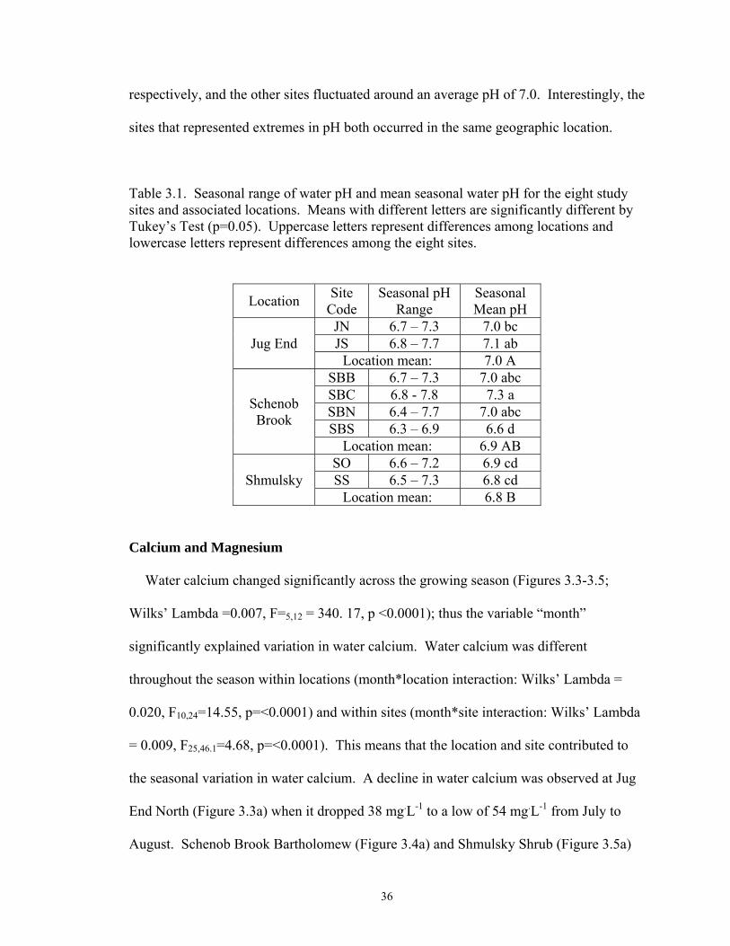
36

respectively, and the other sites fluctuated around an average pH of 7.0. Interestingly, the

sites that represented extremes in pH both occurred in the same geographic location.

Table 3.1. Seasonal range of water pH and mean seasonal water pH for the eight study sites and associated locations. Means with different letters are significantly different by Tukey’s Test (p=0.05). Uppercase letters represent differences among locations and lowercase letters represent differences among the eight sites.

Location Site Code

Seasonal pH Range

Seasonal Mean pH

Jug End JN 6.7 – 7.3 7.0 bc JS 6.8 – 7.7 7.1 ab

Location mean: 7.0 A

Schenob Brook

SBB 6.7 – 7.3 7.0 abc SBC 6.8 - 7.8 7.3 a SBN 6.4 – 7.7 7.0 abc SBS 6.3 – 6.9 6.6 d

Location mean: 6.9 AB

Shmulsky SO 6.6 – 7.2 6.9 cd SS 6.5 – 7.3 6.8 cd

Location mean: 6.8 B

Calcium and Magnesium

Water calcium changed significantly across the growing season (Figures 3.3-3.5;

Wilks’ Lambda =0.007, F=5,12 = 340. 17, p <0.0001); thus the variable “month”

significantly explained variation in water calcium. Water calcium was different

throughout the season within locations (month*location interaction: Wilks’ Lambda =

0.020, F10,24=14.55, p=<0.0001) and within sites (month*site interaction: Wilks’ Lambda

= 0.009, F25,46.1=4.68, p=<0.0001). This means that the location and site contributed to

the seasonal variation in water calcium. A decline in water calcium was observed at Jug

End North (Figure 3.3a) when it dropped 38 mg.L-1 to a low of 54 mg.L-1 from July to

August. Schenob Brook Bartholomew (Figure 3.4a) and Shmulsky Shrub (Figure 3.5a)

37

37

a. b.Jug End - Water Calcium

2006

May 4

May 18

June

10Ju

ne 19

July

6Ju

ly 17

Augus

t 1Aug

ust 1

5Sep

t. 7Sep

t. 21

Oct. 5

Oct. 18

Ca+2

(mg. L-1

)

20

40

60

80

100

120


Jug End - Water Table Depth

2006Apri

l 30

May 4

May 18

June

10Ju

ne 19

July

6Ju

ly 17

Augus

t 1Aug

ust 1

5Sep

t. 7Sep

t. 21

Oct. 5

Oct. 18

wat

er ta

ble

dept

h (c

m)

-70

-60

-50

-40

-30

-20

-10

0

10

Figure 3.3. a. Seasonal variation in water calcium (mg.L-1) at the Jug End location. Each point represents a mean of three replicate samples. b. A comparison with seasonal water table depth.

38

38

a. b.Schenob Brook - Water Calcium

2006

May 4

May 18

June

10Ju

ne 19

July

6Ju

ly 17

Augus

t 1Aug

ust 1

5Sep

t. 7Sep

t. 21

Oct. 5

Oct. 18

Ca+2

(mg. L-1

)

20

40

60

80

100

120Bartholomew (SBB)Schenob Central (SBC)Schenob North (SBN)Schenob South (SBS)

Schenob Brook - Water Table Depth

2006

April 3

0May

4May

18Ju

ne 10

June

19Ju

ly 6

July

17Aug

ust 1

Augus

t 15

Sept. 7

Sept. 2

1Oct.

5Oct.

18

wat

er ta

ble

dept

h (c

m)

-70

-60

-50

-40

-30

-20

-10

0

10

Figure 3.4. a. Seasonal variation in water calcium (mg.L-1) at the Schenob location. Each point represents a mean of three replicate samples. b. A comparison with seasonal water table depth.

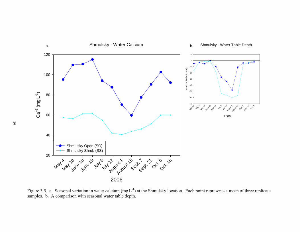
39

39

a. b. Shmulsky - Water Table Depth

2006

April 3

0May

4May

18Ju

ne 10

June

19Ju

ly 6

July

17Aug

ust 1

Augus

t 15

Sept. 7

Sept. 2

1Oct.

5

wat

er ta

ble

dept

h (c

m)

-70

-60

-50

-40

-30

-20

-10

0

10

Shmulsky - Water Calcium

2006

May 4

May 18

June

10Ju

ne 19

July

6Ju

ly 17

Augus

t 1Aug

ust 1

5Sep

t. 7Sep

t. 21

Oct. 5

Oct. 18

Ca+2

(mg. L-1

)

20

40

60

80

100

120


Figure 3.5. a. Seasonal variation in water calcium (mg.L-1) at the Shmulsky location. Each point represents a mean of three replicate samples. b. A comparison with seasonal water table depth.

40

40

were the only sites whose calcium values actually increased mid-season. The remaining

sites, Schenob Brook North and Central (Figure 3.4a) and Jug End North (Figure 3.3a)

maintained steady calcium levels throughout the growing season. The largest seasonal

change in water calcium was observed at Shmulsky Open (Figure 3.5a) where values

dropped steadily by 55 mg.L-1 to a low of 38 mg.L-1 from June to August.

The changes in calcium over the growing season corresponded to characteristics in the

water table during the same time periods (Figures 3.3b, 3.4b, 3.5b). At the locations

where the water table dropped below the depth at which water was collected (30 cm),

groundwater was no longer being sampled directly and thus calcium values were lower as

water chemistry was more reflective of unsaturated pore water equilibria instead of

groundwater conditions.

The seasonal mean water calcium was significantly different among locations

(F2,16=62.21, p =<0.0001 ) and among sites (F5,16=21.70, p=<0.0001) (Table 3.2).

Schenob Brook had calcium values significantly lower than at Jug End and Shmulsky,

which were not different from each other. In general, Shmulsky Open maintained the

highest water calcium with a mean of 92 mg.L-1, and Schenob Brook Central was

consistently the lowest with a seasonal mean of 26 mg.L-1.

41

Table 3.2. Seasonal range of water calcium and mean seasonal water calcium for the eight study sites and associated locations. Means with different letters are significantly different by Tukey’s Test (p=0.05). Uppercase letters represent differences among locations and lowercase letters represent differences among the eight sites.

Location Site Code

Seasonal Calcium (mg.L-1) Range

Seasonal Mean Calcium (mg.L-1)

Jug End

JN 37.0 – 112.5 82.1 ab JS 47.3 – 95.0 78.9 ab


Schenob Brook

SBB 42.5 – 78.5 63.2 bc SBC 16.3 – 37.8 25.7 e SBN 22.0 – 73.5 52.0 cd SBS 22.5 – 52.5 36.9 de


Shmulsky

SO 38.0 – 133.5 92.0 a SS 33.5 – 74.5 52.9 cd


Water magnesium changed significantly across the growing season (Figure 3.6)

(Wilks’ Lambda =0.164, F=5,12 12.27, p= 0.0002); thus the variable “month” significantly

explained the variation in water magnesium. Water magnesium was also significantly

different seasonally within locations (month*location interaction: Wilks’ Lambda =

0.090, F10,24 = 5.57, p=0.0003) and within sites (month*site interaction: Wilks’ Lambda =

0.067, F25,46.1 = 1.98, p=0.0222). This means that the location and site contributed to the

seasonal variation in water magnesium. Shmulsky Open exhibited the largest seasonal

change in water magnesium (Figure 3.6c) where values dropped steadily by 25 mg.L-1

from June to August. Schenob Brook sites Bartholomew and South (Figure 3.6b) and

both Jug End sites (Figure 3.6a) had water magnesium values that increased mid-season.

Of these, Bartholomew remained at the elevated level; South returned to the levels it had

in the spring, and the two Jug End sites initially returned to spring levels but then

increased back to their peak height in October. The other sites, Shmulsky Shrub,

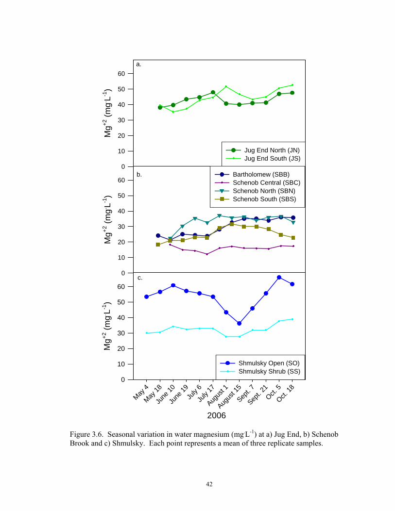
42

Mg+2

(mg. L-1

)

0

10

20

30

40

50

60


Mg+2

(mg. L-1

)

0

10

20

30

40

50

60Bartholomew (SBB)Schenob Central (SBC)Schenob North (SBN)Schenob South (SBS)

2006

May 4

May 18

June

10

June

19Ju

ly 6

July

17

Augus

t 1

Augus

t 15

Sept. 7

Sept. 2

1Oct.

5

Oct. 18

Mg+2

(mg. L-1

)

0

10

20

30

40

50

60


a.

b.

c.

Figure 3.6. Seasonal variation in water magnesium (mg.L-1) at a) Jug End, b) Schenob Brook and c) Shmulsky. Each point represents a mean of three replicate samples.

43

Schenob Brook Central, and Schenob Brook North remained at fairly constant levels

throughout the entire growing season. Seasonal changes in magnesium were similar to

those of calcium, as would be expected since the bedrock underlying many of these sites

contains dolomite. Later, this relationship will be discussed further.

The seasonal mean water magnesium was significantly different among locations

(F2,16=45.02, p =<0.0001 ) and among sites (F5,16= 11.51, p=<0.0001) (Table 3.3).

Schenob Brook had significantly lower magnesium than Jug End and Shmulsky, which

were not different from each other. In general, Shmulsky Open maintained the highest

water magnesium with a seasonal mean of 54 mg.L-1, and Schenob Central was

consistently the lowest with a seasonal mean of 16 mg.L-1.

Table 3.3. Seasonal range of water magnesium and mean seasonal water magnesium for the eight study sites and associated locations. Means with different letters are significantly different by Tukey’s Test (p=0.05). Uppercase letters represent differences among locations and lowercase letters represent differences among the eight sites.

Location Site Code

Seasonal Magnesium

(mg.L-1) Range

Seasonal Mean Magnesium

(mg.L-1)

Jug End

JN 30.0 – 60.5 42.5 ab JS 32.0 – 59.0 44.1 ab


Schenob Brook

SBB 17.5 – 42.5 29.1 c SBC 9.3 – 30.0 16.2 d SBN 14.75 – 42.0 32.7 bc SBS 15.3 – 37.5 24.8 cd


Shmulsky

SO 23.0 – 70.0 54.0 a SS 25.0 – 46.5 32.4 bc


44

Due to the nature of the bedrock surrounding the study sites (predominantly dolomitic

and lesser amounts of calcitic limestone), it is expected that the levels and fluctuations in

calcium and magnesium will correspond to each other if they are all delivered with water

that has traveled through bedrock with the same mineral composition. In fact, trends in

water magnesium across the season do closely follow those of the calcium for each site

(Figure 3.7) but with some variability in the spring months. If the groundwater traveled

mostly through dolomitic limestone, one would expect Ca:Mg to be about 1.74, the

equivalent ratio of the atomic weight of 1 mole of calcium per the atomic weight of 1

mole of magnesium. If the water traveled through calcitic limestone as well as dolomitic

limestone, then greater amounts of calcium would be present and the ratio would be

greater than 1.74.

Overall, seasonal mean significant differences were observed in the Ca:Mg ratios

among the three study locations (F2,16=3.68, p=0.0483) and among the eight study sites

(F5,16=20.92, p=<0.0001) (Table 3.4). Ratios at Jug End were significantly higher

than at Schenob and Shmulsky, which were not different from each other. In addition,

“month” was a significant causative factor affecting seasonal Ca:Mg variation (Wilks'

Lambda =0.031, F5,12=74.73, p=<0.0001) (Figure 3.7). However, these differences were

only marginally significant within locations (month*location interaction: Wilks' Lambda

=0.276, F10,24=2.16, p=0.0586) and not in any way within sites (month*site interaction:

Wilks' Lambda =0.190, F25,46.1=1.04, p= 0.4409). Schenob Brook Bartholomew had the

significantly highest Ca:Mg ratio of all of the sites at 2.12. This elevated ratio would be

expected as it is the only site that is directly down gradient from a purely calcitic

marble/limestone section of bedrock. The sites with the next highest Ca:Mg ratio

45

occurred at Jug End where the surrounding bedrock contained both dolomite and calcite.

The Shmulsky sites fell in the middle as their surrounding bedrock also contained both

dolomite and calcite. The remaining Schenob sites (Central, North and South) had the

lowest range with an average of 1.5, which would also be expected, as the bedrock

surrounding them is chiefly comprised of the mineral dolomite.

Seasonal variation in water Ca:Mg

2006

May 4

May 18

June

10

June

19Ju

ly 6

July

17

Augus

t 1

Augus

t 15

Sept. 7

Sept. 2

1Oct.

5

Oct. 18

Ca+2

:Mg+2

0.0

0.5

1.0

1.5

2.0

2.5

3.0

Jug End NorthJug End SouthBartholomewSchenob CentralSchenob NorthSchenob SouthShmulsky OpenShmulsky Shrub

Figure 3.7. Seasonal variation in calcium to magnesium ratios for the eight study sites. Each point represents a mean of three replicate samples.

46

Table 3.4. Seasonal range of water calcium to magnesium ratios and mean seasonal water calcium to magnesium ratios for the eight study sites and associated locations. Means with different letters are significantly different by Tukey’s Test (p=0.05). Uppercase letters represent differences among locations and lowercase letters represent differences among the eight sites.

Location Site Code

Seasonal Ca:Mg Range

Seasonal Mean Ca:Mg

Jug End

JN 1.41 – 2.31 1.91 ab JS 1.39 – 2.13 1.78 bc


Schenob Brook

SBB 1.96 – 2.60 2.12 a SBC 1.41 – 1.82 1.62 cd SBN 1.41 – 1.93 1.55 cd SBS 1.29 – 1.69 1.47 d


Shmulsky

SO 1.49 – 2.01 1.71 bcd SS 1.27 – 1.91 1.63 bcd

Location mean: 1.67 C

Iron

No distinct trends were observed in water iron (total iron) across the growing season

(Wilks’ Lambda =0.365 F5,9=3.13 p=0.0656). However, there were significant seasonal

differences within locations (month*location interaction: Wilks’ Lambda=0.176, F10,18

=2,49, p=0.0440) and within sites (month*site interaction: Wilks’ Lambda=0.045, F25,

34.9=1.83, p =0.0496) (Figure 3.8). Significant differences existed among the sites in June

(F5,13= 3.11, p=0.0460), and in August among the locations (F2,13 =7.12, p=0.0082) and

among the sites (F5,13=4.23, p=0.0167). Three of the sites at Schenob (Bartholomew,

North and South), and Jug End North, exhibited similar seasonal trends in that the iron

increased in July and August and then declined in the autumn months. One site at each

location, Shmulsky Shrub, Schenob Brook Central, and Jug End South, had very low iron

47

Tota

l Fe

(mg.

L-1 )

0

2

4

6

8

10

12 Bartholomew (SBB)Schenob Central (SBC)Schenob North (SBN)Schenob South (SBS)

2006

May 4

June

10Ju

ly 6

Augus

t 1

Sept. 7

Oct. 5

Tota

l Fe

(mg.

L-1 )

0

2

4

6

8

10

12 Shmulsky Open (SO)Shmulsky Shrub (SS)

Tota

l Fe

(mg.

L-1 )

0

2

4

6

8

10

12 Jug End North (JN)Jug End South (JS)

a.

b.

c.

Figure 3.8. Seasonal variation in water iron (mg.L-1) at the a) Jug End, b) Schenob Brook and c) Shmulsky locations. Each point represents a mean of three replicate samples.

48

levels with no seasonal change. Shmulsky Open exhibited the most unique seasonal

trend in comparison to the others, in that it peaked in June, declined greatly in August,

and increased again in September (but to only half of the peak it exhibited in June).

Differences in the seasonal mean water iron were not explained by location

(F2,13=0.34, p=0.7207), nor were they explained by site (F5,13=2.43, p=0.0919) (Table

3.5). At many observations, iron was undetectable. The greatest amount of iron was

measured during the irregular peak that occurred at Shmulsky Open in which it reached

22 mg.L-1 on June 10th. On average, this site also had the highest mean seasonal iron at

5.3 mg.L-1. Schenob Brook Central was consistently the lowest with a mean seasonal

value of 0.1 mg.L-1.

The variation in iron at Shmulsky Open may be explained by the disconnect from

groundwater (as indicated by hydrologic measurements) that occurred at that site after

June, as well as the loss of strong reducing conditions that occurred in the summer

months (Appendix C). Groundwater may provide a source of iron as the bedrock

surrounding the sites (Figures 1.4, 1.6 and 1.8) contains micaceous schist, a metamorphic

rock with iron-containing silicate minerals (Aldridge and Churchman, 1991). The three

sites that showed no seasonal change had lower iron values in general (Jug End South,

Schenob Brook Central, Shmulsky Shrub) and also had the most oxidizing conditions

throughout the growing season (Appendix C). It is difficult to explain the iron levels at

the remaining sites (Jug End North, Schenob Brook North, Schenob Brook Bartholomew,

Schenob Brook South), where iron was highest during the summer months and was lower

in the spring and fall. For the Schenob sites, the water table remained constant

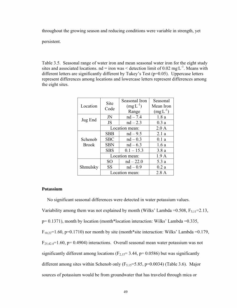
49

throughout the growing season and reducing conditions were variable in strength, yet

persistent.

Table 3.5. Seasonal range of water iron and mean seasonal water iron for the eight study sites and associated locations. nd = iron was < detection limit of 0.02 mg.L-1. Means with different letters are significantly different by Tukey’s Test (p=0.05). Uppercase letters represent differences among locations and lowercase letters represent differences among the eight sites.

Location Site Code

Seasonal Iron (mg.L-1) Range

Seasonal Mean Iron (mg.L-1)

Jug End

JN nd – 7.4 1.8 a JS nd – 2.3 0.3 a


Schenob Brook

SBB nd – 9.5 2.1 a SBC nd – 0.3 0.1 a SBN nd – 6.3 1.6 a SBS 0.1 – 15.3 3.8 a


ShmulskySO nd – 22.0 5.3 a SS nd – 0.9 0.2 a


Potassium

No significant seasonal differences were detected in water potassium values.

Variability among them was not explained by month (Wilks’ Lambda =0.508, F5,11=2.13,

p= 0.1371), month by location (month*location interaction: Wilks’ Lambda =0.335,

F10,22=1.60, p=0.1710) nor month by site (month*site interaction: Wilks’ Lambda =0.179,

F25,42.4=1.60, p= 0.4904) interactions. Overall seasonal mean water potassium was not

significantly different among locations (F2,15= 3.44, p= 0.0586) but was significantly

different among sites within Schenob only (F5,15=5.85, p=0.0034) (Table 3.6). Major

sources of potassium would be from groundwater that has traveled through mica or

50

feldspar minerals (Brady, 1999) or from fertilizer input. Thus potassium may be supplied

to the wetlands by groundwater that has traveled through the micaceous schists

surrounding the sites (Figures 1.5 and 1.7) or from adjacent agriculture. These results

may indicate that farming played a large role as Shmulsky Open and Schenob Brook

Bartholomew had the highest potassium values and were also in closest proximity to

various forms of agriculture (e.g. vegetable production, and cattle farms). Schenob

Brook Bartholomew was adjacent to vegetable fields and Shmulsky Open was adjacent to

cattle grazing areas.

Table 3.6. Seasonal range of water potassium and mean seasonal water potassium for the eight study sites and associated locations. Means with different letters are significantly different by Tukey’s Test (p=0.05). Uppercase letters represent differences among locations and lowercase letters represent differences among the eight sites.

Location Site Code

Seasonal Potassium

(mg.L-1) Range

Seasonal Mean Potassium (mg.L-1)

Jug End JN 0.4 – 2.7 0.9 bc JS 0.6 – 2.3 1.4 abc


Schenob Brook

SBB 1.5 – 3.1 2.0 a SBC 0.7 – 2.1 1.3 abc SBN 0.4 – 3.1 1.7 ab SBS 0.5 – 2.8 0.9 bc


Shmulsky SO 0.5 – 3.9 1.5 abc SS 0.3 – 1.5 0.7 c


51

Ammonium and Orthophosphate

Seasonal variability in ammonium (Wilks’ Lambda =0.322, F3,9=2.25, p= 0.0971) and

orthophosphate (Wilks’ Lambda =0.450, F5,9=2.20, p= 0.144) were not observed in this

study, nor were seasonal differences detected among sites (ammonium: Wilks’ Lambda

=0.251, F15,25.3=1.09, p= 0.4079; orthophosphate: Wilks’ Lambda =0.118, F25,34.9=1.08,

p= 0.406) or locations (ammonium: Wilks’ Lambda =0.336, F6,18=2.17, p= 0.095;

orthophosphate: Wilks’ Lambda =0.384, F10,18=1.10, p= 0.410). The average amount of

ammonium in the pore water was 0.4 mg.L-1 (expressed as ammonium, NH4+) but ranged

from undetectable levels to 3.0 mg.L-1 at Shmulsky Open (Table 3.7). Orthophosphate

was present in the pore water at an average concentration of 0.11 mg.L-1 (expressed as

phosphate, PO43-) but ranged from undetectable levels to 1.63 mg.L-1 at Schenob Brook

Bartholomew (Table 3.8). Due to the proximity of most of these sites to various forms of

agriculture it was expected that ammonium and orthophosphate levels would be elevated

from fertilizer or manure inputs. Corresponding with findings for elevated potassium,

both Shmulsky Open and Schenob Brook Bartholomew (the sites in closest proximity to

agricultural land uses) had the highest ammonium and orthophosphate of all of the sites

studied. At Shmulsky Open, the peaks in these nutrients occurred in May. This may

have coincided with spring fertilizer applications at other locations in the watershed. At

Bartholomew these peaks occurred in August (ammonium) and October (orthophosphate)

and could be related to increased nitrogen mineralization when temperatures were

warmer and/or fall fertilizer applications.

52

Table 3.7. Seasonal range of water ammonium and mean seasonal water ammonium for the eight study sites and associated locations. nd = ammonium was < detection limit of 0.02 mg.L-1. Means with different letters are significantly different by Tukey’s Test (p=0.05). Uppercase letters represent differences among locations and lowercase letters represent differences among the eight sites.

Location Site Code

Seasonal ammonium

(mg.L-1) Range

Seasonal Mean ammonium

(mg.L-1)

Jug End JN nd – 1.81 0.36 a JS nd – 0.52 0.13 a


Schenob Brook

SBB nd – 2.08 0.57 a SBC nd - 0.86 0.14 a SBN nd – 1.42 0.31 a SBS nd – 1.83 0.56 a


Shmulsky SO nd – 3.02 0.86 a SS nd – 0.50 0.17 a


Table 3.8. Seasonal range of water orthophosphate and mean seasonal water orthophosphate for the eight study sites and associated locations. nd = orthophosphate was < detection limit of 0.02 mg.L-1. Means with different letters are significantly different by Tukey’s Test (p=0.05). Uppercase letters represent differences among locations and lowercase letters represent differences among the eight sites.

Location Site Code

Seasonal orthophosphate (mg.L-1) Range

Seasonal Mean orthophosphate

(mg.L-1)

Jug End JN nd – 1.19 0.18 a JS nd – 0.50 0.12 a

Location mean: 0.15A

Schenob Brook

SBB nd – 1.63 0.17 a SBC nd – 0.96 0.09 a SBN nd – 0.20 0.04 a SBS nd – 0.30 0.08 a


Shmulsky SO nd – 1.36 0.13 a SS nd – 0.13 0.05 a


53

Soil Analysis

Detailed accounts of the physical and chemical properties of the soil at each study

plot and for each horizon to a depth of 60cm are available in Appendix E. The following

results and discussion refer to the surface soil horizons at each of the study sites unless

otherwise stated. Overall, the soil physical and chemical properties differed among sites

(Wilks' Lambda = 0.0006, F45,38.9= 3.68, p=<0.0001) and among locations (Wilks'

Lambda = 0.009, F18,16= 8.25, p=<0.0001).

Soil Physical Properties

In general, soils had mucky, organic rich surface horizons and mineral subsurface

horizons. The texture of the subsoil varied among the study sites from sand, loamy sand,

sandy loam, loam, to silt loam although the majority of the subsurface soils were

reflective of their outwash nature as being either loamy sands or sandy loams. Only at

Schenob Brook South were all soil samples silt loams. This observation was not

surprising as this was the only site comprised of alluvial deposits from the nearby

Schenob Brook.

Percent organic matter varied from 8.7% at Schenob Brook Central to 75% at Schenob

Brook North. It differed significantly among locations (F2,16=6.63, p=0.0080) and among

sites within locations (F5,16=7.75, p=0.0007) (Table 3.9). The Schenob location was

significantly higher than Jug End, but neither of them were significantly different from

Shmulsky. Considering that the water table at Schenob never dropped below 30cm, it

makes sense that organic matter accumulation would be high. Thus some portion of the

surface soils at all of the Schenob sites was saturated during the entire growing season,

allowing less decomposition of organic matter as compared to better aerated sites.

54

54

Table 3.9. Soil physical and chemical properties for the eight study sites within the three locations. Measurements are represented on a per weight basis. Each number represents a mean of three soil samples collected from three soil pits (one at each plot) at each site. Means with different letters are significantly different by Tukey’s Test (p=0.05). Uppercase letters represent differences among locations and lowercase letters represent differences among the eight sites.

Location Site pH Organic Matter

(% by wt.)

Total N (mg.kg-1)

AB-DTPA Extractable

Elements (pH 7.6) (mg.kg-1)

Exchangeable cations (NH4OAc, pH 7) (mg.kg-1)

P Fe Ca Mg K Fe

Jug End

JN 7.3 ab 14.0 bc 5646 bc 1.1 a 99.0 cd 3132 b 335.7 cd 39.6 a 0.7 a JS 7.5 a 11.1 c 4653 c 1.3 a 63.9 bd 2649 b 289.7 d 31.5 a 0.8 a

Mean 7.4 A 12.5 A 5150 A 1.5 A 81.5 A 2891 A 312.7 A 35.6 A 0.7 A

Schenob

SBB 7.0 abc 17.1 bc 7630 abc 2.0 a 137.5 bcd 3914 b 459.8 bcd 59.1 a 1.4 a SBC 6.8 abc 10.6 c 3620 c 2.1a 89.4 cd 2483 b 335.2 cd 41.9 a 2.8 a SBN 6.4 bc 51.1 a 14843 a 2.5 a 267.0 ab 7968 a 1204.1 a 90.8a 3.7 a SBS 6.1 d 35.0 ab 14323 ab 4.2 a 401.3 a 5232 a 780.9 b 216.6 a 6.8 a Mean 6.5 B 26.6 B 10104 B 2.7 B 222.3 B 4900 B 695.0 B 104.7 B 3.7 B

Shmulsky

SO 6.4 bc 26.1 abc 10513 abc 1.8 a 162.7 abc 4907 b 681.8 bc 36.4 a 1.3 a SS 6.8 abc 13.9 bc 6246 abc 1.3 a 127.1 bcd 2926 b 401.4 cd 34.8 a 1.1 a

Mean 6.6 B 20.0 AB 8380 AB 1.2 A 144.9 B 3916 AB 541.6 B 35.6 A 1.2 B

55

55

The differences in organic matter affected the method of reporting of the soil nutrients.

When represented on a per weight basis the concentration of an element in mg.kg-1 was

more representative of the amount of organic matter in the sample than the actual

concentrations per volume of soil. For this reason, the bulk density was measured for

each of the soils so that the nutrient measurements could be standardized on a volume

basis. Nutrient measurements as a function of weight are presented in Table 3.9. The

following discussion of the soil chemical properties will only refer to the nutrient

measurements that are on a volume basis which are reported in Table 3.10.

In general, bulk densities ranged from 0.34 g.cm -3 for the soils that contained large

amounts of organic matter to 0.96 g.cm-3 for those with less. Significant differences in

bulk density were detected among locations (F2,16= 10.34, p=<0.0001) and among sites

(F5,16=7.98, p=0.0009) (Table 3.10). The bulk density at Schenob was significantly lower

than at Jug End and Shmulsky, which were not different from each other.

Soil Chemical Properties

Similar trends were observed for pH, calcium, and magnesium in the soil, as were

observed in the water chemistry. Soil pH ranged from 6.1 at Schenob Brook South to 7.5

at Jug End South. Significant differences in pH were observed among locations

(F2,16=11.14, p=0.0009) and among sites within locations (F5,16=2.91, p=0.0467) (Table

3.9). The soil pH at Jug End was significantly higher than at Schenob and Shmulsky,

which were not different from each other. Significant differences in soil calcium were

observed among locations (F2,16=7.97, p=0.0256) and among sites within locations

(F5,16=10.62 p=0.0137) (Table 3.10). When grouped by location, the soil calcium at

56

56

Table 3.10. Physical and chemical properties for surface soils at the eight study sites within the three locations, expressed on a volume basis. Each number represents a mean of three soil samples collected from three soil pits (one at each plot) at each site. Means with different letters are significantly different by Tukey’s Test (p=0.05). Uppercase letters represent differences among locations and lowercase letters represent differences among the eight sites.

Location Site Bulk

Density (g.cm-3)

Organic Matter (kg.m-3)

Total N (g.m-3)

AB-DTPA Extractable Elements

(pH 7.6) (g.m-3)

Exchangeable cations (NH4OAc, pH 7) (g.m-3)

P Fe Ca Mg K Fe

Jug End

JN 0.84 a 113.2 bc 4557 ab 0.9 a 82.7 b 2528 ab 272.7 b 32.0 a 0.6 a

JS 0.84 a 95.2 c 3977 ab 1.1 a 55.8 b 2254 ab 247.6 b 27.2 a 0.7 a

Mean 0.84 A 104.2 A 4266 A 1.0 A 69.2 A 2390 A 260.1 A 29.6 A 0.6 A

Schenob

SBB 0.76 ab 125.0 bc 5559 ab 1.4 a 97.1 ab 2885 ab 336.8 ab 43.5 a 1.1 a

SBS 0.48 bc 161.0 a 6559 a 1.9 a 179.9 a 2423 ab 361.9 ab 99.1 a 3.1 a

SBC 0.71 ab 74.2 bc 2507 b 1.4 a 61.2 b 1724 b 235.8 b 28.6 a 1.9 a

SBN 0.34 c 143.0 a 4922 ab 0.8 a 89.6 b 3112 a 470.3 a 38.3 a 1.4 a

Mean 0.57 B 125.8 AB 4886 A 1.4 A 106.9 AB 2536 A 351.2 B 52.4 A 1.9 B

Shmulsky

SO 0.73 ab 188.5 ab 7576 a 1.3 a 119.0 ab 3541 a 489.3 a 26.0 a 0.9 a

SS 0.96 a 130.9 bc 5874 ab 1.2 a 120.9 ab 2744 ab 376.5 ab 32.2 a 1.1 a

Mean 0.84 A 160.0 B 7088 B 1.2 A 120.0 B 3142 B 432.9 C 29.1 A 1.0 A

57

57

Shmulsky was significantly higher than Schenob and Jug End, which were not different

from each other. Schenob Brook Central had the lowest soil calcium at 1554 g.m -3 and

Shmulsky Open had the highest at 3680.3 g.m -3. Significant differences existed in soil

magnesium among locations (F2,16=16.41, p=0.0003) and among sites (F5,16=16.47,

p=0.0015) (Table 3.10). All three locations were significantly different from each other.

Although water analyses did not show significant differences in nitrogen (as

ammonium) and iron (as total iron), significant differences were observed in total

nitrogen and in DTPA-iron in the soil. Total nitrogen was significantly different among

locations (F2,16=4.80, p=0.0132) and among sites within locations (F5,16=5.75, p=0.0234)

(Table 3.10). This same trend was also observed in % organic matter (by wt.) suggesting

that the nitrogen pool is controlled directly by the contribution from organic matter.

Total nitrogen at Shmulsky was significantly higher than at Schenob and Jug End, which

were not different from each other. Differences in exchangeable iron were only observed

among locations (F2,16= 7.14, p=0.0370) as Jug End was significantly lower than Schenob

and Shmulsky, which were not different from each other. Significant differences in

DTPA iron were observed among locations (F2,16=12.68, p=0.0334) and among sites

within locations (F5,16= 7.43, p=0.0071) (Table 3.10). Schenob was not different from

Jug End or Shmulsky, both of which were different from each other. Again, Jug End had

the lowest iron levels. This trend makes sense considering that both Schenob and

Shmulsky had significant amounts of micaceous schist (a rock with iron-containing

silicates) in the surrounding bedrock and Jug End had very little. Thus groundwater

would be more likely to carry iron to those sites where it could be stored in exchangeable

forms on soil colloids and in amorphous precipitates.

58

Soil phosphorus and potassium were not significantly different among sites but were

significantly different among locations when compared on a weight basis. These

differences then were most likely due to differences in the amount of organic matter at

those sites. Large differences were not expected for soil phosphorus as it did not differ in

the water analysis, however it was somewhat surprising to see that soil potassium values

were not different as they were in the water analysis. Although there were no significant

differences, soil potassium ranged from 22 to 99 g.m -3 and this may reflect the observed

differences in its water chemical values.

General Chemical Properties

Water chemistry at Shmulsky corresponded with those found by Picking (2002) at the

same location. Levels of water ammonium, orthophosphate, iron, and soil phosphorus

potassium, magnesium, and percent organic matter fell within the expected range. Even

similar maximum iron levels were observed in the water at Shmulsky (22 mg.L-1). It was

surprising to observe orthophosphate levels above 1 mg.L-1, (especially in soils with a pH

above 7) as this is often only associated with heavily fertilized soils (Brady, 1999). Thus

the proximity of these sites to agricultural land must result in a large input from

fertilizers.

Seasonal trends in calcium also corresponded with Picking (2002) who observed high

water calcium in April and May which then dropped to almost half of its original

concentration in the mid-summer months when the water table dropped. Maximum

calcium values corresponded to Picking’s study in 1997 where water calcium never

exceeded 120 mg.L-1 and also to research by Komor (1994) who measured values up to

128 mg.L-1. Shmulsky is an interesting site, because most research on calcareous fens has

59

determined the average range of dissolved calcium (even in what is defined as a “rich

fen”) of being much lower (only 5 to 65 mg.L-1 ). Jug End had a range of 37 to 112.5

mg.L1 calcium and sites at Schenob ranged from 16.3 to 73.5 mg.L-1. The mid-range of

calcium values at these sites were similar to those as studied by Motzkin (1994), and

Slack et al. (1980). Picking (2002) observed soil calcium values to range from 2126 g.m-3

to 4907 g.m -3 at Shmulsky, which corresponded to Shmulsky Open where calcium values

were the highest measured in the current study (3541 g.m -3; although maximum values in

this study were lower).

Overall, the strongest and most significant difference in the chemistry of the waters

and soils of the calcareous fens was due to the differences that could be associated with

calcareous groundwater inputs (i.e., calcium, magnesium, and pH). Minor differences

were observed in the primary macronutrients. The strongest significant difference in

primary macronutrients was observed in total soil nitrogen, although this difference may

be a reflection of the differences in organic matter content among the sites. Phosphorus

was never significantly different and potassium showed significant yet small differences

in the water only. Although water iron was not significantly different among sites or

locations, it showed significant seasonal differences. In the soil, differences were only

observed from the AB-DTPA iron analysis in which much more iron was chelated. This

analysis may have been able to detect those seasonal differences that alone were not

significantly different, by giving an indication to the available pool of iron.

Hydrology – Geochemistry Relationships

Calcium and magnesium did not always show similar trends, and sites with the highest

magnesium values did not necessarily also have the highest calcium values. This would

60

indicate that there are different sources of water entering the wetland locations.

Observing the Ca:Mg ratio seems to support this, as sites whose surrounding bedrock was

comprised of more calcite in relation to dolomite also had less magnesium in relation to

calcium and thus Ca:Mg ratios above 1.74. It was expected that the different locations

would have different sources of groundwater as they were geographically separated from

one another. However, without modeling the groundwater flow-paths these statements

are purely conjecture.

The site with the highest recorded calcium value and overall average highest calcium

levels (Shmulsky Open) also had the most continuous upwelling of groundwater. By

contrast, the two sites with the lowest average water calcium values (Schenob Brook sites

Central and South) were the only two sites that showed repeated recharge conditions

throughout the growing season. These findings support the notion that the major source

of calcium entering these wetlands is groundwater and that when water moving from the

substratum to the surface is substantial (i.e., when the wetland is in direct contact with the

groundwater) the surface waters will have elevated calcium levels. When a site only

receives water that flows laterally from other areas of strong upwelling or when those

flow-through sources are diluted by surface water, the calcium levels in the wetlands

appear to be much lower.

This trend was particularly evident at Shmulsky, where the water table dropped

sharply in mid-summer at both sites, but only Shmulsky Open had a significant drop in

water calcium. Shmulsky Open generally had very high calcium levels and continuous

upwelling whereas the other site, Shmulsky Shrub, had neither upwelling nor recharge

and maintained overall lower calcium levels. Thus, Shmulsky Shrub was receiving a

61

supply of calcium only after it had flowed through the soil and attained an equilibrium

with it. Thus when Shmulsky Open stopped receiving groundwater inputs, the water

calcium values dropped to the levels present at Shmulsky Shrub and most likely soil

equilibrium levels.

In general, the sites that exhibited the largest change in water calcium during the

growing season, Shmulsky Open and Jug End South, also exhibited the largest drop in

water table depth. These two changes occurred simultaneously during the warm dry

summer months from June to August when groundwater was no longer in contact with

the 30cm sampling depth. By contrast, the sites that maintained fairly constant water

tables throughout the growing season (Schenob Brook sites) also had stable water

calcium values.

Conclusions

The hydrologic properties of eight calcareous fens sites in Massachusetts were not

alike; however, the differences were attributable to calcium and magnesium enrichment

in the wetland waters and the level at which those elements varied across the growing

season. Significant differences in water and soil calcium, magnesium, and pH were

observed among study sites and among locations, as were differing trends in water table

depth and vertical groundwater gradients. Interestingly, water table depth and vertical

groundwater gradients could not be correlated to each other as it was determined that

sites were receiving water through different mechanisms (directly upwelling or lateral

flow from upwelling zones). The level of upwelling seemed to control the average water

calcium level, but the fluctuation in the water table seemed to govern how that calcium

varied across the season.

62

Although the main focus of this study, as reported in the next chapter, was to

document plant patterns and associations with soil calcium, it is important to remember

that the observed plant distribution patterns may be in response to many environmental

variables other than calcium. By establishing that the strongest environmental gradients

in these calcareous fens are those related to the calcareous bedrock geochemistry, i.e.,

calcium, magnesium, and pH, and that in fact other minor gradients do exist, i.e., nitrogen

and iron, a better understanding of the suspected gradients underlying individual species

can be achieved.

63

CHAPTER IV

PLANT COMMUNITY ANALYSIS

Introduction

Naturalists have long been interested in the unique plant communities that develop in

soils enriched with calcium (Sendtner, 1860; Contejean, 1881; Bonnier, 1894; Kerner von

Marilaun, 1895; Schrimper, 1898; and many others). Recent studies have focused on the

plant communities in calcareous fens (Vitt et al., 1975, Slack et al., 1980; Komor, 1994;

Motzkin, 1994; Bedford et al, 1999; Picking and Veneman, 2004) where elevated

calcium levels exist due to upwelling groundwater that has traveled through calcareous

bedrock. These studies have identified unique plant communities that are associated with

the geochemical properties of calcareous fens, i.e., elevated calcium and magnesium

levels, elevated pH, and low phosphorus availability relative to noncalcareous fens. No

two fens are identical with respect to these conditions and thus overall plant communities

differ among fens. Little research has yet focused on these differences at the species

level; however, literature reports indicate that some fen species occur only at significantly

elevated levels of calcium whereas others appear to occur across a wide range. Within

these occurrences, plants can be quite abundant or occur infrequently depending on their

life cycles. In addition, not all species occurring in the fens are specific to those calcium-

loving communities; common wetland plants also occur there as well.

This chapter will focus on organizing species of northeastern calcareous fens into

groups based on literature reports of their rarity and affinity for calcium. These

groupings are used in subsequent chapters to test hypotheses regarding the distribution

and physiology of calciphiles in relation to environmental calcium levels (see Chapter 1).

64

In addition, this chapter presents the findings of the vegetation survey conducted across

eight calcareous fen research sites in three locations in the Berkshire-Taconic region of

Massachusetts, including a characterization of the plant communities observed as well as

analysis of the species diversity among sites. Species richness was analyzed in terms of

the soil N:P ratio to test the hypothesis by Bedford et al. (1999) that fen ecosystems

generally have high species richness as they are limited by phosphorus.


Vegetation Survey

The vegetation survey was conducted from July 10 to 21, 2006. This timeframe was

selected to maximize potential for identifying graminoid species, many of which were

flowering during this period. Three vegetation sampling plots were established at each of

the eight field sites, and each plot was associated with a water-sampling station.

Vegetation distribution was sampled in a 2.5-m radius plot positioned at the center point.

This specific size provided a sampling area of 19.6 m2, which exceeds the minimum

sampling area that was developed using a species area curve for similar habitats (Picking,

2002). Plant species occurring within the plots were identified, and their percent cover

was estimated visually.

A Priori Species Selection

A list of species was compiled from the three most recent studies of Massachusetts

calcareous fen vegetation (Motzkin, 1994; Kearsley, 1999; Picking and Veneman, 2004)

to determine species with which to test hypotheses regarding the distribution and

physiology of calciphiles in relation to environmental calcium levels. These studies all

65

conducted vegetation surveys and measured a general substrate calcium level associated

with the fens where the plants occurred. Species were grouped based on their abundance

in relation to substrate calcium levels into one of three categories. Species placed in

Category 1 were species determined to be rare or indicator species in high-calcium fens;

Category 2 species were dominant or characteristic in high-calcium fens and Category 3

represented species common to a wide range of fen calcium levels, including common

wetland plants. Species in a priori category groupings were compared with species

actually observed at the research sites.

Species Richness and Turnover

Presence-absence data from the vegetation survey were used to calculate species

richness at each 19.6 m2 plot and collectively at each site (58.8m2). A regression analysis

was conducted (SAS Version 9.1.3, SAS Institute, 2004) to assess if the species richness

correlated with the ratio of total soil nitrogen to AB-DTPA-extractable phosphorus (see

Chapter 3 for method details). Non-normal data were log-transformed prior to analysis.

Presence-absence data from the vegetation survey also were used to calculate species

turnover by estimating the similarity between each plot and between each site.

Sørensen's distance matrix (Sørenson/Bray-Curtis distance measure calculated in PC-

ORD Ver. 5) was subtracted from 1 to calculate a similarity index (McCune and Mefford,

1999). This index provided an estimate of the number of species shared between plots

and between sites.

66


Community Characterization

One hundred thirty-three vascular plant species were observed in total of which 28

were woody, 58 were herbaceous, 7 were ferns and allies, and 40 were graminoids. A

complete species list is included in Appendix F along with species nomenclature

authorities (as they are not included in the text of this manuscript). Species observations

correspond with previous studies of calcareous fen vegetation in Western New England

(Reschke, 1990; Weatherbee and Crow, 1992; Motzkin, 1994; Kearsley, 1999; Picking,

2002). The vegetation at Shmulsky Open, Jug End North and Jug End South appear to be

similar to the “Sloping Graminoid Fen Communities” (after Weatherbee and Crow,

1992), “Calcareous Sloping Fens” (after Kearsley, 1999) or “Rich Sloping/graminoid

Fens” (after Reschke, 1990) where sedges dominate the site with a mixture of smaller

forbs and shrubs. This community type also corresponds with Motzkin’s (1994) Group

III Carex interior-C. leptalea-C. flava type. Sites Shmulsky Shrub and Schenob Brook

Bartholomew appear to be “Shrub Fen” (after Weatherbee and Crow, 1992) or “Rich

Shrub Fen” (after Reschke, 1990) communities as they are in a somewhat transitional

state where shrubs are beginning to dominate. Schenob Brook Central would be

described as a “Calcareous Seep Community” where cold calcareous water seeps to the

surface and forms small rivulets (after Weatherbee and Crow, 1992). The vegetation at

Schenob Brook North appears to be more closely related to a “Lake Basin Graminoid Fen

Community” even though this area may not have formed from a former lake. It is

characteristic of a community that has peat accumulation and elements of graminoid fens,

shrub fens, and bog vegetation (after Weatherbee and Crow, 1992). Schenob Brook

67

South is the only site that would be considered a non-rich fen. According to Reschke

(1990), this site would be called a “Medium Fen” containing many common wetland

species but still having a minerotrophic groundwater influence.

Species Composition: A Priori Groupings

Three categories of plants were established to identify species with different suspected

needs for or tolerances to calcium. All of the selected species occurred in fens with

elevated calcium levels but some species were notably absent or occurred at only low

frequencies when lower levels of calcium existed. Species placed in Category 1 included

species that were considered to be either “rare” or “indicator species” in the high-calcium

wetlands (Table 4.1). It is assumed that these species may be the most important to study

since they occur in limited amounts and usually only in highly calcareous environments.

Six species in this category are listed as endangered, threatened, or of special concern in

Massachusetts (MNHESP, 2004). Category 2 includes species that are considered

“dominant” or “characteristic” species in the high-calcium fens. Although they are not

endangered, threatened, or of special concern, these species are important because they

are abundant and provide the dominant vegetative makeup of the calcareous fens and

appear to occur only at more elevated calcium levels. Category 3 contains both calciphile

and non-calciphile species that appear to occur independent of environmental calcium

levels in calcareous fens. Two of these species (Carex granularis and Dasiphora

fruticosa) are known calciphiles (Gleason and Cronquist, 1991), and because they are

generalists as to their calcium selectivity, will provide a useful comparison to calcium

specialists (from Categories 1 and 2) with respect to calcium accumulation in tissues.

The remaining three species in this category (Symphyotrichum puniceum var. puniceum,

68

Scientific Name † Common Name Status MA+

Category 1 Carex sterilis 1, 2, 3 Carex tetanica 2, 3 Cypripedium parviflorum var. parviflorum 2 Equisetum fluviatile 1 Equisetum scirpoides 2, 3 Eriophorum gracile 2 Geum rivale 1, 3 Juncus nodosus 1 ,2 Lobelia kalmii 1, 2, 3,4 Petasites frigidus var. palmatus 2, 3 Solidago uliginosa 1, 4 Spiranthes romanzoffiana 1, 2

Dioecious sedge Rigid sedge Lesser yellow ladies slipper Water horsetail Dwarf scouringrush Slender cottongrass Water avens Knotted rush Kalm’s lobelia Arctic sweet coltsfoot Northern bog goldenrod Hooded ladies tresses

T

SC E

SC

E

E Category 2 Carex flava 1, 2, 3 Carex hystericina 1, 2, 3 Carex interior 2, 3 Carex leptalea 1, 2, 3 Juncus brachycephalus 1 Packera aurea 1 Parnassia glauca 1, 2, 3, 4 Solidago patula 1, 2, 3

Yellow sedge Bottlebrush sedge Inland sedge Bristly stalked sedge Smallhead rush Golden ragwort Fen grass of Parnassus Roundleaf goldenrod

Category 3 Carex granularis 1, 3, 4 Dasiphora fruticosa ssp. floribunda 1, 2, 3, 4 Symphyotrichum puniceum var. puniceum 1 Symplocarpus foetidus 1 Thelypteris palustris 1, 2, 3

Limestone meadow sedge Shrubby cinquefoil Purplestem aster Skunk cabbage Eastern marsh fern

Table 4.1. A priori species category groupings. Category 1: Rare or indicator species in fens with high calcium levels. Category 2: Dominant or characteristic species in fens with high calcium levels. Category 3: Species that are common fen species across a range of calcium levels. _

1 Picking and Veneman (2004) 2 Kearsley (1999) 3 Motzkin (1994) 4 Species known for growth in calcareous regions by Gleason and Cronquist (1991) † All nomenclature follows USDA (2007) + Species status derived from MNHESP (2004). E = Endangered, T= Threatened, SC=Special Concern

69

Symplocarpus foetidus, and Thelypteris palustris) are common wetland species (non-

calciphiles) that show no selectivity as to environmental calcium levels. Studying this

group will be useful in determining whether calcium tissue storage patterns are unique to

calciphiles or if non-calciphiles also show similar responses to environmental calcium

levels.

Of the 25 species in the a priori categories, 20 were observed in the study plots.

Species not observed were Cypripedium parviflorum Salisb. var parviflorum, Equisetum

scirpoides Michx., Eriophorum gracile L., Petasites frigidus (L.) Fries var. palmatus

(Ait) Cronq., and Spiranthes romanzoffiana Cham. The absence of these species is not

surprising as they represent the rarest of the species from the category as three are

endangered and one is of special concern in Massachusetts (Table 4.1). A cottongrass

similar to E. gracile, Eriophorum viridicarinatum was observed. Similarly, the orchid

relative of S. romanzoffiana, Spiranthes cernua was observed.

Species Richness and Turnover

Among each plot, species richness varied from 16 species at Jug End South (JS2) to 52

species at Shmulsky Open (SO3) (Table 4.2). Thirty species occurred at each plot on

average. Among all of the sites, Schenob Brook South had the lowest total species

richness with 37 species and Jug End North had the highest with 79 species (Table 4.2).

Picking (2002) studied some of the same wetland locations (including the Shmulsky fen)

and recorded species richness values from 55 to 80 species per 15-m2 sampling plot.

Picking's "Station 2" corresponded to a location very close to the Shmulsky Open site (D.

Picking, Pers. Comm.) and at this station, Picking observed a maximum of 68 species per

15-m2 plot. Thus, it was not surprising to see that Shmulsky Open had the highest

70

species richness of any other study plot, and when all three plots at Shmulsky Open were

combined, species, richness was almost identical to Picking's maximum value at 67

(Table 4.2). The general species richness values for the other sites compared with fen

richness values reported by Bedford et al. (1999) who observed between 26 to 78 species

per 25-m2 plot in fens of New York State.

Table 4.2. Species richness at each study plot and cumulative for each study site.

For each site, combined species richness was always greater than when viewed as

individual plots. This trend was the most extreme at Jug End North where total site

Site Plot Richness Site Total

Jug End North

JN1 32 79 JN2 34

JN3 20

Jug End South

JS1 23 39 JS2 16

JS3 27

Bartholomew SBB1 32

50 SBB2 31 SBB3 34

Schenob Central

SBC1 22 43 SBC2 28

SBC3 26

Schenob North

SBN1 29 52 SBN2 38

SBN3 33

Schenob South

SBS1 17 37 SBS2 18

SBS3 25

Shmulsky Open

SO1 34 67 SO2 42

SO3 52

Shmulsky Shrub

SS1 37 57 SS2 33

SS3 40

71

richness was more than double the maximum value observed at an individual plot (Table

4.2). This finding implies that few species are shared among those plots, which is

indicative high β-diversity and high species turnover. Similarity indices were developed

to explore this trend further. Species similarity was compared among plots (Table 4.3)

and among sites (Table 4.4). Values closer to 0 represent extreme dissimilarity and

values closer to 1 indicate identical species composition.

On average, plots shared 38.5% of the same species. This value is quite low but

makes sense considering that some plots occurred in sites that were geographically

separated and that were also determined to be different fen types. Replicate plots shared

more species with each other than with plots in other sites (Table 4.3). On average,

replicate plots within the same site shared 59% of the same species. The lowest

similarity observed within replicate plots was between Jug End North-3 and Jug End

North-2 where they shared only 44% of their species. The strongest overall similarity

was observed between two replicate plots, Schenob Brook North-3 and Schenob Brook

North-2, in which they shared 79% of their species. Much lower similarity existed when

non-replicate plots from different sites were compared. Most notably, the plots at

Schenob Brook South did not share one similar species with Schenob Brook Central-1.

This finding is interesting as these two sites occurred in the same geographic location;

however, Schenob Brook Central was characterized as a "Calcareous Seep Community"

and Schenob Brook South was characterized as a "Medium Fen". These two types of

fens have very different geochemical properties, and so it is not surprising that these two

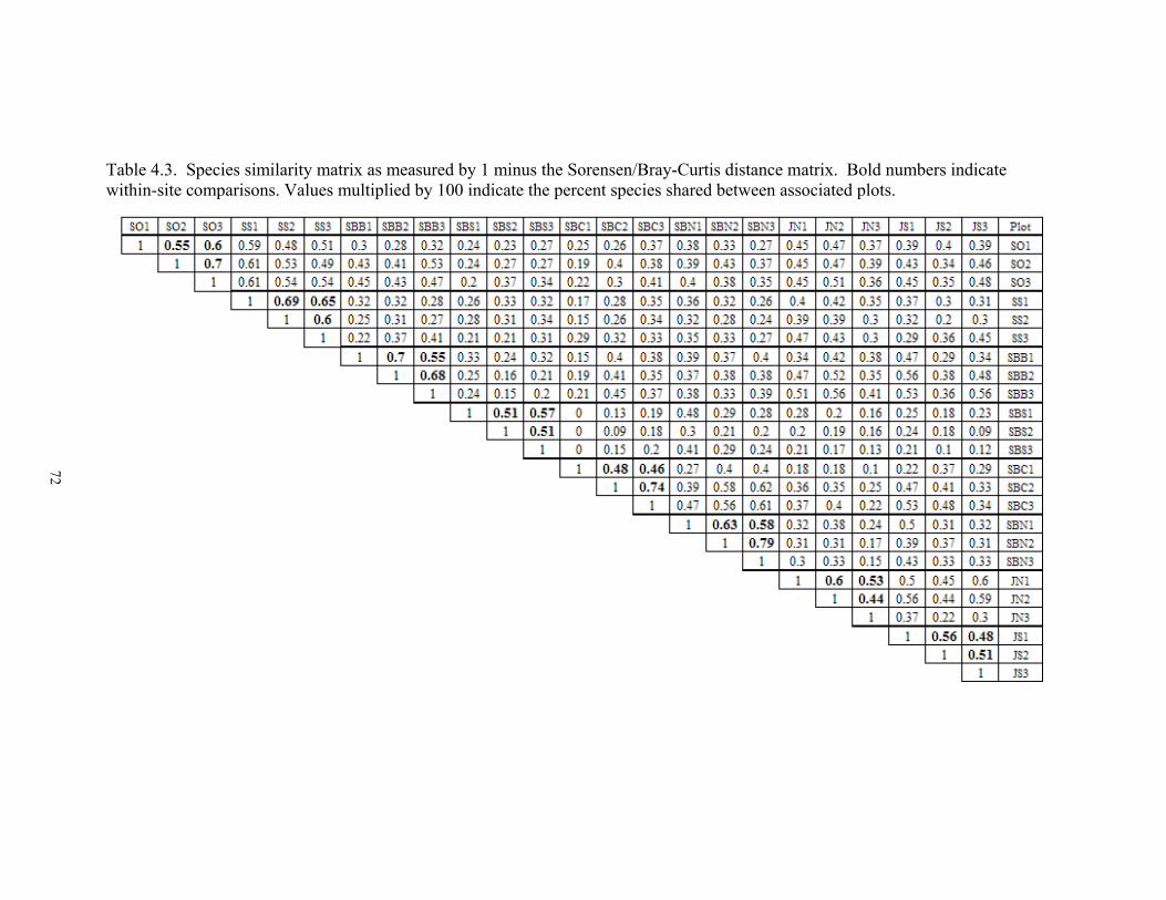
72

72

Table 4.3. Species similarity matrix as measured by 1 minus the Sorensen/Bray-Curtis distance matrix. Bold numbers indicate within-site comparisons. Values multiplied by 100 indicate the percent species shared between associated plots.

73

73

communities had very different species compositions. On average, plots had only 34%

species in common with plots that occurred at different sites.

When plots are combined and species similarity is reported on the site level, similar

trends are observed as with plots (Table 4.4) although species similarity is higher overall.

Highest similarity within geographic locations was observed at Shmulsky and at Jug End

where these sites had 69% and 73% species in common within each location,

respectively. The Schenob sites had fewer species in common. Schenob Brook Central

had only 18% of its species in common with Schenob Brook South, and this distribution

corresponded to the comparison of similarity among plots. Of the Schenob sites, the

greatest number of shared species were between Schenob Brook North and Schenob

Brook Central (60%). Even though Schenob Brook North had vegetation similar to a

"Lake Basin Fen" and Schenob Brook Central was a "Calcareous Seep", they both

occurred adjacent to each other and in similar landscape positions.

Table 4.4. Species similarity matrix as measured by 1 minus the Sorensen/Bray-Curtis distance matrix comparing overall sites (58.8m2). Bold numbers indicate within-location comparisons. Values multiplied by 100 indicate the percent species shared between associated sites.

74

The lack of similarity within sites indicates high species turnover as is associated with

multiple environmental gradients (Picking, 2002). Although rare plants are limited by

factors other than nutrient availability, (i.e. competition, unique pollination strategies,

etc.) significant differences in environmental gradients over small areas allow for more

species with different niches to establish. In Chapter 3, it was determined that there were

strong differences within and among sites. Not only were the primary fen-defining

elements (e.g. calcium, magnesium and pH) significantly different among the sites, but

also differences were observed in hydrology, groundwater upwelling, percent organic

matter, dissolved potassium, as well as DTPA soil iron and total soil nitrogen. These

differences among sites may contribute to differences in plant species composition

however, these additional findings suggest that there may also be significant

environmental differences within sites to account for the high species dissimilarity there.

High species turnover in calcareous fens also was observed by Picking (2002); however,

Picking's plot and site similarity were much greater than observed in this study. This

difference may have been because Picking's (2002) study involved comparisons within

one fen region (the Shmulsky location) whereas the current study viewed three different

geographic locations.

Bedford et al. (1999) reported species richness to be correlated to the ratio of total soil

nitrogen to total soil phosphorus. When conditions become more nutrient rich

(increasing phosphorus levels), species that thrive under nutrient-rich conditions out-

compete the smaller, less robust species (Drexler and Bedford, 2002). The opposite

occurs in phosphorus-limited environments, allowing many more specialized plants to

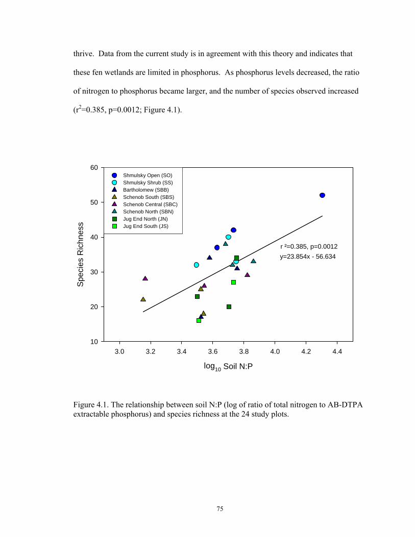
75

thrive. Data from the current study is in agreement with this theory and indicates that

these fen wetlands are limited in phosphorus. As phosphorus levels decreased, the ratio

of nitrogen to phosphorus became larger, and the number of species observed increased

(r2=0.385, p=0.0012; Figure 4.1).

log10 Soil N:P

3.0 3.2 3.4 3.6 3.8 4.0 4.2 4.4

Spec

ies

Ric

hnes

s

10

20

30

40

50

60Shmulsky Open (SO)Shmulsky Shrub (SS)Bartholomew (SBB)Schenob South (SBS)Schenob Central (SBC)Schenob North (SBN)Jug End North (JN)Jug End South (JS)

r ²=0.385, p=0.0012y=23.854x - 56.634

Figure 4.1. The relationship between soil N:P (log of ratio of total nitrogen to AB-DTPA extractable phosphorus) and species richness at the 24 study plots.

76

These results concur with what Bedford et al. (1999) observed in a study of New York

fens. It was interesting to see that this trend was the same because the current study used

a different technique for measuring soil phosphorus as compared to Bedford et al. (1999)

and other previous related studies. It did not seem ecologically meaningful to measure

total phosphorus in the soil (as Bedford did) as much of that is not readily available to

plants. Instead, the AB-DTPA extraction method was selected in this study because it is

buffered at a pH of 7.6 so that it is a realistic representation of potentially available

phosphorus in calcareous fen environments (Jones, 2001). Total nitrogen was measured

as all common forms of nitrogen (organic, nitrate, and ammonium) could be readily

available depending on mineralization and denitrification rates. Thus, absolute N:P ratios

are higher than Bedford's because measurements of extractable phosphorus are naturally

lower than total phosphorus. Even though the ratios differ, the relationships to species

richness are similar.

Conclusions

Even though study plots were established before the majority of vegetation emerged in

April, the species list generated from this study indicates that many common species of

calcareous fens were observed. Out of the total 133 species observed, 20 were of the 25

species selected in the a priori category groupings. The eight sites represented several

different types of calcareous fens as described from previous literature, with only one

being considered a non-rich fen. Species richness varied among the 19.6m2 plots from a

low of 16 species to a maximum of 52 species and corresponds to expected richness

values for vascular species of calcareous fens. Species richness was significantly higher

when plot richness was combined on the site level. Similarity matrices confirmed that on

77

average only 59% of species are in common between adjacent plots. This high species

turnover may be indicative of the multiple environmental gradients present in the sites as

determined in Chapter 3. Species richness increased log-based linearly as did the N:P in

the soil, suggesting that these wetlands are limited by phosphorus and that large, strong

nutrient-loving competitors are absent and greater numbers of smaller, less nutrient

demanding species are able to coexist.

78

CHAPTER V

VEGETATION AND ENVIRONMENTAL GRADIENTS

Introduction

The plant communities associated with calcareous fens have been described as some

of the rarest in North America (Eggers and Reed, 1987). The species that occur in them

are specifically adapted to the unique geochemical conditions, namely elevated soil and

water pH, calcium, and magnesium (Slack et al., 1980; Vitt and Chee, 1990; Komor,

1994; Motzkin, 1994; Kearsley, 1999; Picking and Veneman, 2004; Bowles et al., 2005).

Motzkin (1994), in a study of western New England fens, established species groupings

that have been since used and validated by other researchers (Kearsley, 1999; Picking and

Veneman, 2004) to describe the vegetation. These species groupings were correlated

significantly to differences in environmental properties, with depth to the mineral soil

being the most important, but also with pH, calcium, and magnesium in the fen surface

waters. Vitt and Chee (1990) reported a strong correlation between vegetation

composition and fen pH, calcium, magnesium, and electrical conductivity in their study

of water and peat chemistry in fens of Alberta, Canada. Generalizations have been made

as to the types of vegetation communities that are associated with certain levels of water

calcium and pH, although few studies have used these findings to focus on the

requirements and distributions of individual species in relation to these geochemical

factors.

In this chapter, ordination analyses are used to discern where differences in species

abundance patterns may exist in relation to site geochemical properties. By identifying

trends in environmental calcium levels and identifying where species-abundance patterns

79

correlate to these underlying calcium gradients it may be possible to determine if certain

species increase in abundance as calcium levels increase or whether species occur only

above a specific calcium threshold. For these species, calcium ranges and thresholds

were identified as to the suspected environmental calcium levels required by these plants.


Data Analysis

The Bray-Curtis (Polar) Ordination with three axes (following variance-regression

endpoints (Beals, 1984), Sørenson’s distance measure and Euclidean projection

geometry) was used to view patterns in species distributions and environmental variables

in relation to the study plots. The ordinations were carried out using multivariate

statistical software (PC-ORD Ver. 5, McCune and Mefford, 1999). A general

relativization was performed prior to these analyses to normalize the data and then a

Mantel Test (Douglas and Endler, 1982) was conducted to compare the original data

matrix to the transformed data matrix. A p=<0.05 assured that the transformed matrix

did not deviate in trends with the original data structure.

The overlay function in PC-ORD was used to assess the correlations that existed

between one set of raw variables and the underlying ordination. For the environmental

data ordination, this procedure was accomplished by setting the normalized

environmental variables as the main matrix and then using the “overlay” function to view

the raw vegetation abundance data (from a secondary matrix) as they correlated to the

underlying ordination scores. Similarly, to view the strong underlying environmental

gradients, the raw environmental data were overlaid on the main transformed

environmental matrix, and resulting axes of correlation and coefficients were recorded.

80

The same procedure was used for the vegetation ordination. Results of the correlation

were assessed visually in the form of joint plots and scatter plots with a Pearson's linear

correlation coefficient (r) calculated for each variable. The direction of the vector in the

joint plot indicates the direction of the correlation with the underlying axis to which it is

parallel. The length of the vector indicates the strength (Pearson's r) of the correlation

relationship.

The locations of the 24 study plots were chosen based on the expected vegetation that

they would contain, and thus inferential statistics cannot be applied to analyses including

them as individual points, as the analysis would be violating the assumptions that the

variables are independent of each other. Nevertheless, the 24 plots were ordinated simply

to view trends in the similarity among them in relation to their vegetative community

structure. More reliable inferences were derived from the ordination of the

environmental data, in which the plots were selected without bias with respect to their

substrate characteristics.

The environmental data set used in the ordination of the environmental properties

included 40 environmental variables organized by the 24 plots. For water chemistry data,

the mean, median, minimum, and maximum concentration for each element were

included if those elements where shown to change across the growing season (Chapter 3).

For elements with no seasonal differences, only the means were used. Soil properties

were measured only once, and thus one single representation of each soil measure was

used in the data set. For the ordination of the vegetation, species that occurred in fewer

than three plots were removed. This reporting resulted in a matrix of the abundance

81

measurements of 85 species organized by the 24 plots. These 85 species are noted in

Appendix F.

For species where the ordination indicated they were correlated to an environmental

gradient, a regression analysis (SAS Ver. 8.1.3 - SAS Institute, 2004) compared the

abundance of that species to that environmental property. Data were transformed by log

or square root for normality prior to analysis. Graphs present results for untransformed

data; however, the statistics are based on the normalized values.

Species Distribution Patterns

Species that appeared to change significantly along the axes where calcium gradients

were significant were considered gradient species, and the numerical range of water

calcium in which it occurred was noted. Species whose abundance correlated

significantly with calcium gradients (even if it was a low correlation) but occurred only at

an extreme of the ordination (where calcium was highest), were considered threshold

species. This distribution implied that these species occurred only when calcium values

reached a certain elevated level. Once a species of this threshold nature was identified,

the lowest calcium values at which the species occurred was reported.


Vegetation Community Analysis

The distribution patterns of the eighty-five species generated a matrix in which plots

were arranged in “species space” (Figure 5.1). Plots are displayed only as they were

arranged on Axis 1 and Axis 3 due to the very low significance of Axis 2 (r2=0.020).

Collectively, Axis 1 and Axis 3 explain 29.3% of the variation in species distribution

82

Figure 5.1. Two-dimensional (Axis 1 and Axis 3) ordination of study plots represented in species space. r2= 0.293 for all variables shown (Axis1: r2=0.123, Axis3: r2=0.170). Larger distances between plots represent greater dissimilarity in species composition at those plots. Symbols are coded by location (shapes), and site (colors). Refer to legend in Figure 4.1 for full clarification.

patterns. The axes represent the range of ordination scores assigned to each plot as

computed from the vegetation abundance at each of those plots. Thus plots that occurred

farthest from each other had the most dissimilar species community structure, and those

that occurred closer to one another were more similar in plant species populations. Not

surprisingly, the three plots from each study site were grouped closer to each other than

they were to plots in other sites. Likewise, the sites that occurred within the same

location were grouped closer to each other than to those from different locations.

SO1

SO2

SO3SS1

SS2

SS3

SBB1

SBB2SBB3

SBS1

SBS2

SBS3

SBC1

SBC2SBC3

SBN1

SBN2SBN3

JN1

JN2

JN3JS1

JS2

JS3

Species Space

Axis 1

Axis

3

83

Schenob Brook Bartholomew, Shmulsky Open and Schenob Brook Central appeared to

be quite similar in species community structure as they are clustered in the center of the

diagram (Figure 5.1). The Jug End sites (Jug End North and Jug End South) are

separated on Axis 3, and are on the opposite end of Axis 3 to Schenob Brook South.

Schenob Brook North and Shmulsky Shrub are separated on opposite ends of Axis 1.

These findings correspond with the Sørenson's distance matrices calculated from

presence-absence data for the plots (Chapter 4). Plots that shared very few species by

Sørenson's distance matrix were also more distant from each other in species space. In

addition, the sites that were very dissimilar by Sørenson's distance matrix, Jug End North

and Schenob Brook South, are on opposite ends of Figure 5.1. Sites that were very

similar, Shmulsky Open and Shmulsky Shrub, and Jug End North and Jug End South are

clustered nearby each other in Figure 5.1. The Bray-Curtis ordination uses Sørenson's

distance matrix to calculate its ordination scores, and so by definition, these findings are

consistent.

Individual species with linear correlations (r2 > 0.4) to the underlying axes are

presented in the joint plot in Figure 5.2 and are listed with significant axes of correlation

and Pearson’s r values in Table 5.1. Because this ordination is in "Species Space" these

strongly correlated species are largely responsible for the underlying plot distribution in

the resulting ordination. Two major, and three minor groups of species can be identified

as being responsible for the separation among the plots. Six species (Alnus serrulata,

Calopogon tuberosus, Glyceria grandis, Larix laricina, Pogonia ophioglossoides, and

Toxicodendron vernix) group on the left side of Figure 5.2 and are all negatively

correlated with Axis 1. These species were thus more common at Schenob Brook North

84

Figure 5.2. Joint plot of species with linear correlations (r2 > 0.4) to species space (see Table 5.1). Symbols are coded by location (shapes), and site (colors). Refer to legend in Figure 5.1 for full clarification.

and less abundant at Shmulsky Shrub. By contrast, Fraxinus pennsylvanica is positively

correlated with Axis 1 and has the opposite distribution to the previously discussed

group.

The second largest group includes the four species, Impatiens capensis, Poa palustris,

Polygonum sagittatum, and Rosa multiflora. These are all positively correlated with Axis

3 and were more common in Schenob Brook South and less abundant in the Jug End

sites. Opposite these species are Dasiphora fruticosa and Parnassia glauca, which are

ALNSER FRAPENLARLAR

DASFRU

ROSMUL

TOXVER

CALPUL

IMPCAP

PARGLA

POGOPH

POLSAGPOAPAL

GLYGRA

Species Space

Axis 1

Axis

3

85

Table 5.1. Species with correlations of r2 > 0.4 to the underlying vegetation matrix. This table corresponds to Figure 5.2. Species ID Code Axis Pearson’s r Alnus serrulata ALNSER 1 -.659 Calopogon tuberosus var. tuberosus CALTUB 1 -.639 Dasiphora fruticosa DASFRU 3 -.736 Fraxinus pennsylvanica FRAPEN 1 .724 Glyceria grandis GLYGRA 1 -.633 Impatiens capensis IMPCAP 3 .821 Larix laricina LARLAR 1 -.698 Parnassia glauca PARGLA 1, 3 .439, -.613 Poa palustris POAPAL 3 .715 Pogonia ophioglossoides POGOPH 1 -.688 Polygonum sagittatum POLSAG 3 .758 Rosa multiflora ROSMUL 3 .652 Toxicodendron vernix TOXVER 1 -.638

negatively correlated with Axis 3 and were more abundant in the Jug End sites.

Parnassia glauca is unique however because it is also positively correlated with Axis 1.

When the raw environmental data were overlaid on the underlying vegetation matrix

(Figure 5.3, Table 5.2), four main groups of environmental correlations were observed.

pH (water and soil), and minimum piezometric gradients were correlated negatively with

Axis 3. A second group included numerous soil measurements (percent organic matter

and soil nitrogen, phosphorus, iron, potassium and magnesium), which were positively

correlated with Axis 3. These correlations were not surprising since an increase in pH

usually results in a decrease in available iron and phosphorus. On Axis 1 a third group

was correlated negatively and included median water potassium and weeks of constant

saturation in the spring. In addition to Axis 3, a fourth trend was observed in which

minimum water calcium was positively correlated with Axis 1 in addition to being

negatively correlated to Axis 3.

Species and environmental properties that were correlated on the same axis suggest

86

Figure 5.3. Joint plot of environmental variables with linear correlations (r2 > 0.2) to species space (see Table 5.2). Symbols are coded by location (shapes), and site (colors) (see Figure 5.1). that those species were responding to those particular environmental properties. Alnus

serrulata, Calopogon tuberosus, Glyceria grandis, Larix laricina, Pogonia

ophioglossoides, and Toxicodendron vernix were all negatively correlated with Axis 1, in

which "weeks of constant saturation in the spring" was also. It is not surprising that these

species would be responding to a hydrologic gradient as all of these plants are considered

to be facultative wetland to obligate wetland species (USDA, 2007). What is more

interesting however is that many of these species are associated with “bog vegetation”

CaMinKmedian

WaterpH

SoilMg

SoilFeSoilKSoilFeDT

SoilNOM

SoilpH

SoilP

consatsp

PieMin

Species Space

Axis 1

Axis

3

87

Table 5.2. Ordination results for environmental variables with linear correlations with r2 > 0.2 to the underlying vegetation matrix. This table corresponds to Figure 5.3. Variable ID Code Axis Pearson’s r Calcium Minimum – Water CaMin 1, 3 .485, -.336 Groundwater gradients, minimum PieMin 3 -.498 Iron – Soil SoilFe 3 .618 Iron DTPA – Soil SoilFeDT 3 .758 Magnesium - Soil SoilMg 3 .475 Nitrogen - Soil SoilN 3 .658 Organic matter – % OM 1, 3 -.517, .558 pH – Soil SoilpH 3 -.617 pH – Water12 WaterpH 3 -.681 Phosphorus - Soil SoilP 3 .611 Potassium – Soil SoilK 3 .654 Potassium Median – Water Kmedian 1 -.466 Saturation – spring, Weeks of continuous consatsp 1 -.601

(Weatherbee, 1996; Mitch and Gosselink, 1993). This association would be accurate as

bog areas are continually inundated and species that occur in them are highly adapted to

such wet and potentially anoxic conditions. In addition, the area where these species

were more abundant, Schenob Brook North, (but also at Schenob Brook Central) is

similar to the “lake basin” type fen (Chapter 4) that had a large amount of organic matter

accumulation and where the water table never dropped below the surface (Chapter 3) and

where it is not uncommon for bog vegetation to be present.

Impatiens capensis, Poa palustris, Polygonum sagittatum, and Rosa multiflora were

all correlated positively with Axis 3. The same relationship was observed for the percent

organic matter and the soil chemistry. These findings imply that plots where these

species were more abundant had greater levels of these elements and also had lower pH

as pH was negatively correlated with Axis 3. Upon further inspection, it is clear that

12 Mean, median, minimum and maximum water pH all showed similar correlations to Axis 3. For simplicity, water pH is shown as one line on the joint plot and the mean water pH correlation is reported.

88

these species were not abundant across the 24 plots, but all only occurred in three or

fewer plots mainly in the Schenob Brook South fen. Schenob Brook South was the only

fen in this study that was determined to be a "medium fen", indicating that it had a lower

average pH and lower calcium levels. Thus these species are a reflection of a wetland

with weaker calcareous qualities with elevated primary nutrient levels, elevated iron and

lower pH. By contrast sites on the opposite side of Figures 5.2 and 5.3 represent species

and environmental characteristics typical of a calcareous fen. Species correlated to this

region were Dasiphora fruticosa and Parnassia glauca.

Dasiphora fruticosa was the only species to be negatively correlated with Axis 3, in

which the ordination pattern is strongly controlled by soil and water pH. This suggests

that pH may have a strong role in the abundance of this species and that it increases as pH

does. Parnassia glauca was the only species that was positively correlated to Axis 1 and

negatively correlated to Axis 3. These correlations correspond directly to only one

environmental property: minimum water calcium. Thus it appears that this species may

be dependent upon the minimum calcium value at each plot.

The ordination of the plots in species space revealed interesting relationships among

the plots and their associations with species and environmental properties. Only 29.3%

of the data were represented by the two axes. While this may appear low, separating 30%

- 50% of the “signal” from the “noise” is considered adequate when conducting

ordinations on data sets of 20 or more species (McCune and Grace, 2002).

It was anticipated that more species would be strongly associated with environmental

calcium levels (the calciphiles), yet only one species (Parnassia glauca) showed this

pattern and only one other showed a relationship with pH (Dasiphora fruticosa). Instead,

89

species significantly correlated with this underlying ordination seemed to be more

associated with hydrologic gradients or to lower pH levels. This result seems to imply

that by viewing plots in terms of species abundance, a few very strong species respond to

hydrologic gradients and the effects of calcium and pH on the vegetation patterns remain

largely unexplained. Perhaps the low level of explanation of these underlying axes is

unable to detect minor differences within plant distributions and only the larger more

obvious differences (i.e., hydrology) are teased out. To circumvent this problem, the

environmental properties were themselves ordinated to see how the vegetation compared

when it was overlaid on the environmental ordination matrix. This approach allows finer

scale differences in the environmental properties to become more apparent since the

ordination was driven by those environmental properties.

Environmental Data Analysis

The axes of the ordination for the environmental properties explain quite a bit more

variation among plots than did the vegetation ordination. The three-dimensional

ordination in environmental space explains 79% of the variation in the data set. Figure

5.4 shows the distribution of the study plots in “environmental space”.

Across all three axes, Schenob Brook North, Jug End South, Shmulsky Shrub and

Schenob Brook Bartholomew are clustered in the center of the diagram (Figure 5.4),

indicating that those sites are more similar in overall environmental properties as

compared to the more distant sites. Shmulsky Open plots 1 and 2 occur on the opposite

end of Axis 1 from where the Schenob Brook Central plots occur. Thus on Axis 1 these

plots represent extremes in environmental property differences. On Axis 2, Schenob

Brook South-3 occurs at the opposite end to Jug End North-1. Axis 3 mainly represents

90

90

a. b.

Figure 5.4. Three-dimensional ordination of study plots represented in environmental space. a) Axis 1: r2=0.531 and Axis 2: r2= 0.141, b) Axis 1: r2=0.531 and Axis 3: r2= 0.120. Cumulative r2=0.792. Larger distances between plots represent greater dissimilarity in species composition at those plots. Symbols are coded by location (shapes), and site (colors); refer to legend in Figure 4.1.

SO1

SO2SO3

SS1SS2

SS3 SBB1

SBB2

SBB3

SBS1

SBS2

SBS3

SBC1

SBC2

SBC3

SBN1

SBN2

SBN3

JN1

JN2

JN3

JS1 JS2

JS3

Environmental Space

Axis 1

Axis

2

SO1

SO2

SO3

SS1

SS2

SS3

SBB1

SBB2

SBB3

SBS1

SBS2

SBS3

SBC1

SBC2

SBC3

SBN1

SBN2

SBN3

JN1

JN2

JN3

JS1JS2

JS3

Environmental Space

Axis 1

Axis

3

91

91

the distinction of the Schenob Brook Central-1 and Schenob Brook Bartholomew-3 from

the other plots.

It is notable that larger differences exist in environmental properties among plots

within the same site than were observed by differences in vegetation. Although plots

within sites mostly group together, their distribution is farther spread than with the

vegetation ordination. Some plots (e.g. Shmulsky Open-3) stand alone far from where

the other replicate plots at that site are distributed. In addition, sites that occur within the

same geographic location are widely separated. Shmulsky Open and Shmulsky Shrub are

at opposite ends of Axis 1. This is interesting as originally it was thought that sites in the

same geographic location would have similar environmental properties. These

differences are in agreement with findings in Chapter 4 where the overall community

characterization indicated that sites within locations were different types of fen

communities. These findings are most important in that they validate the concept that the

environmental variables, to some degree, were independent of the observable vegetation

patterns (as was a previously mentioned concern with analyzing pseudoreplicates).

The significance of the explanatory variables used to generate the environmental

matrix are presented in Table 5.3. Individual environmental properties with linear

correlations (r2 > 0.4) to the underlying axes are presented in the joint plots in Figure 5.5.

Because this ordination is in "Environmental Space" these strongly correlated

environmental properties are largely responsible for the underlying plot distribution in the

resulting ordination. On Axis 1 (albeit weakly), water iron and ammonium are correlated

positively and water pH is negatively correlated. All water calcium and magnesium

measurements are correlated positively with Axis 1, and these, along with maximum

92

Table 5.3. Environmental variables included in the main matrix of the ordination analysis with Pearson’s r for axes of correlation (corresponds to Figure 5.5).

Variable ID Code Pearson’s r for Axis: 1 2 3

Ammonium Mean – Water NMean .784 Calcium – Soil CaSoil .515 -.630 Calcium Maximum – Water CaMax .411 -.707 -.416 Calcium Mean – Water CaMean .333 -.727 -.472 Calcium Median – Water CaMedian .333 -.706 -.492 Calcium Minimum – Water CaMin -.756 -.428 Groundwater gradients, maximum PieMax .603 -.410 Groundwater gradients, mean PieMean -.304 -.429 Groundwater gradients, median PieMedian .559 -.527 Groundwater gradients, minimum PieMin -.311 -.309 Iron – Soil FeSoil .716 .309 Iron DTPA – Soil FeDTPASo .423 .534 Iron Maximum – Water FeMax .904 Iron Mean – Water FeMean .912 Iron Median – Water FeMedain .897 Iron Minimum – Water FeMin .735 Magnesium – Soil MgSoil .580 -.511 Magnesium Maximum – Water MgMax .412 -.596 -.437 Magnesium Mean – Water MgMean .391 -.639 -.515 Magnesium Median – Water MgMedian .389 -.666 -.466 Magnesium Minimum – Water MgMin -.550 -.548 Nitrogen – Soil NSoil .524 .643 -.303 Organic Matter – % OM .459 .644 pH – Soil pHSoil -.390 -.520 pH Maximum – Water pHMax -.659 pH Mean – Water pHMean -.634 pH Median – Water pHMedian -.604 pH Minimum – Water pHMin -.451 -.417 Phosphorus – Soil PSoil .452 Phosphorus Mean – Water PMean -.505 Ponding, Total weeks of Totpond -.632 Ponding, Weeks of continuous ConPond -.589 Potassium – Soil KSoil .664 Potassium Maximum – Water KMax .471 Potassium Mean – Water KMean low correlation Potassium Median – Water KMedian low correlation Potassium Minimum – Water KMin low correlation Saturation – fall, Weeks of continuous Consatfall .309 -.562 Saturation – spring, Weeks of continuous Consatsp .342 -.437 Saturation, Total weeks of Totsat .300 -.571

93

93

a. b.

Figure 5.5. Joint plot of environmental properties with linear correlations (r2 > 0.4) to environmental space on a) Axis 1 and Axis 2 and b) Axis 1 and Axis 3 (see Table 5.3). Symbols are coded by location (shapes), and site (colors). Refer to legend in Figure 5.4.

CaMinCaMaxCaMeanCaMedian

MgMeanMgMedian

NmeanFeMeanFemin Femax

FeMedian

pHMaxpHMean

SoilFeSoilK

SoilNOM

Environmental Space

Axis 1

Axis

2

NmeanFeMean

Femin FemaxFeMedianpHMax

pHMean

SoilCa

SoilMg

totpondPieMedia

PieMax

Environmental Space

Axis 1

Axis

3

94

94

groundwater gradients, are negatively correlated to Axes 2 and 3. The variables strongly

and positively correlated with only Axis 2 are soil iron and soil potassium but percent

organic matter and soil nitrogen are strongly positively correlated to both Axes 1 and 2.

Total weeks of ponding is negatively correlated with Axis 3.

In summary, two major groups of environmental differences appear to separate the

plots. Plots that are distributed in either the positive direction on Axes 1 or 2 have higher

levels of water and soil iron and nitrogen and by contrast, those in the negative direction

on Axis 1 have higher water pH. Although the micaceous schist may be a significant

contributor of iron in groundwater, it appears from Figure 5.5a that exchangeable soil

iron was less where pH was greatest. This makes sense considering that elevated pH

values associated with alkalinity from upwelling groundwater would drive iron into

amorphous (non-exchangeable) precipitates. Plots that are distributed in the negative

direction of Axis 1 and 3 appear to be strongly influenced by upwelling groundwater that

has traveled through carbonate bedrock. This is evidenced by the correlation of these axes

to various hydrogeochemical factors, i.e., water pH (Axis 1 only), groundwater gradients,

total weeks of ponding and both the water (Axis 1 only) and soil calcium and magnesium.

Axis 1

Species that were correlated on the same axis as underlying environmental variables

may be responding to those particular environmental properties (Table 5.4). In the

positive direction on Axis 1, where water iron and ammonium cause separation of the

plots, species such as Thelypteris palustris, Equisetum fluviatile, Juncus effusus,

Calamagrostis canadensis, Populus tremuloides, and Sium suave (Figure 5.6) were more

abundant. Although these species may be responding to increased water iron and

95

Table 5.4. Species correlations (r2 > 0.2) to the underlying environmental matrix (corresponds to Figure 5.6).

∗ Denotes species from a priori category groupings.

Species ID Code Pearson’s r for Axis: 1 2 3

Amphicarpaea bracteata AMPBRA .617 Betula papyrifera BETPAP .617 Calamagrostis canadensis CALCAN .492 -.306 Carex granularis* CARGRA -.494 Carex stricta CARSTR .524 Coptis groenlandica COPGRO -.318 .624 Dasiphora fruticosa *∗ DASFRU -.572 -.444 Equisetum fluviatile* EQUFLU .690 -.324 Equisetum hyemale EQUHYE -.318 .624 Gallium asprellum GASASP .617 Impatiens capensis IMPCAP .655 Juncus effusus JUNEFF .419 -.462 Juniperus communis JUNCOM -.318 .624 Muhlenbergia glomerata MUHGLO -.448 Osmunda cinnimonea OSMCIN .626 Packera aurea* PACAUR -.462 Parnassia glauca* PARGLA -.742 Parthenocissus quinquefolia PARQUI .617 Poa palustris POAPAL .409 .574 Polygonum sagittatum POLSAG .538 Populus tremuloides POPTRE .498 Rubus pubescens RUBPUB .500 Sium suave SIUSUA .498 Sphagnum sp. SPHAG -.399 .614 Thelypteris palustris* THEPAL .478 -.307 Trientalis borealis TRIBOR -.318 .624 Vaccinium corymbosum VACCOR -.322 .523 Viburnum dentatum VIBDEN -.487

96

96

a. b.

Figure 5.6. Joint plot of species with linear correlations (r2 > 0.2) to environmental space on a) Axis 1 and Axis 2 and b) Axis 1 and Axis 3 (see Table 5.4). Symbols are coded by location (shapes), and site (colors). Refer to legend in Figure 5.4.

BETPAP

POPTREDASFRU

RUBPUB

VIBDEN

AMPBRA

GALASPIMPCAP

PARGLA

PARQUI POLSAG

SIUSUA

EQUFLUTHEPAL

CARGRA

JUNEFFMUHGLO

CALCAN

Environmental Space

Axis 1

Axis

2

CARSTR

POAPAL

PACAUR

POPTRE

DASFRU

VACCORCOPGRO

JUNCOM

SIUSUA

TRIBOR

EQUFLU

EQUHYEOSMCIN

THEPAL

CALCAN

SPHAG

Environmental Space

Axis 1

Axis

3

97

97

ammonium, they may also be responding to lower water pH levels, as water pH had a

negative correlation (in the opposite direction) with Axis 1. Only Dasiphora fruticosa

had a negative correlation with Axis 1, and thus appears to increase as water pH does.

Except for Equisetum fluviatile, none of the species positively correlated with Axis 1 are

established calciphiles but they are all species adapted to moist conditions, waste places,

or to both (Weatherbee, 1996). This response reflects their distribution as generalists that

are not selecting habitats with increased calcareous nature. Auclair (1979) reported that

Equisetum fluviatile had elevated concentrations of iron in its tissues. Thus the

correlation of this species to water iron may be directly related with its ability to tolerate

elevated iron levels.

Axis 2

Parnassia glauca, Packera aurea, Viburnum dentatum, Muhlenbergia glomerata, and

Carex granularis had strong negative correlations with Axis 2 where water and soil

calcium and magnesium were correlated. By contrast Carex stricta, Rubus pubescens,

Polygonum sagittatum, Betula papyrifera, Gallium asprellum, Amphicarpaea bracteata,

Parthenocissus quinquefolia, Poa palustris, and Impatiens capensis were positively

correlated with Axis 2 where percent organic matter and soil iron, nitrogen and potassium

were positively correlated. Collectively, these findings imply that the former group (with

Parnassia glauca, etc.) increases in abundance with increasing water calcium and

magnesium and is less abundant where there is more organic matter and soil iron,

nitrogen and potassium. This finding reinforces the nature of the three species, Parnassia

glauca, Packera aurea, and Carex granularis as calciphiles. Although not included in

the original category groupings, Muhlenbergia glomerata is also known to be common in

98

calcareous fens (Weatherbee and Crow, 1992). By contrast, the latter group (with Carex

stricta, etc.) increases in abundance with increasing organic matter and soil iron and

decreases where water calcium and magnesium are greater. Many species in this group

are common wetland species (USDA, 2007) and thus it was not expected for them to

occur in areas with strong calcareous influences, but it was expected that they would

occur in response to a hydrologic gradient. Their increase in response to increasing

organic matter may reflect this as organic matter accumulation is indicative of long-term

saturation.

Axis 3

Soil calcium, magnesium and groundwater gradients were strongly negatively

correlated with Axis 3 and several species appeared to respond to the opposite trend,

increasing where groundwater gradients and soil calcium and magnesium were lower.

These species included Vaccinium corymbosum, Coptis groenlandica, Juniperus

communis, Trientalis borealis, Equisetum hyemale, Osmunda cinnamomea, and

Sphagnum sp. These findings suggest that these species occurred where calcareous

inputs, e.g. soil calcium, magnesium, and groundwater input, were lower. Vaccinium

corymbosum, Trientalis borealis, and Coptis groenlandica are reported by Weatherbee

(1996) as occurring in acidic soils in Berkshire County, Mass. and sphagnum moss is a

well-known inhabitant of acidic substrates (Robichaud and Anderson, 1994).

The Schenob Brook Central and Schenob Brook South sites are distributed in the same

region on Axis 3 in the direction where these species are correlated. Schenob Brook

South was characterized by having low calcium, magnesium, pH and low upwelling of

groundwater as well as high iron levels. However, Schenob Brook Central shared those

99

same characteristics except that it had the highest water pH of any of the sites and had

hardly any iron. Because Schenob Brook Central was a "calcareous seep" it had many

rivulets that separated ~0.35-m high hummocks where the plants were growing. The soil

pH in these hummocks was much lower than the water pH (around 6.6 compared to 7.6)

and may explain this distribution. These acidophiles (acid loving plants) could also be

responding to components that were not measured in this study, such as alkalinity, which

would be lower where there was less groundwater input and where calcium and

magnesium levels were lower.

Summary

In general, the results of both the ordinations of species distributions and

environmental parameters seem to indicate that one general theme describes plant

distributions. Species seem to either be related to increases in calcareous inputs (calcium,

magnesium, pH, and groundwater upwelling) or increases in iron, which may reflect a

decrease in calcareous inputs. Six species from the a priori category groupings were

observed, in which all except Equisetum fluviatile increased in abundance in relation to

higher calcareous inputs. More variation in plots was explained by the environmental

ordination than the vegetation ordination and this may be why more species appeared to

be patterned with the underlying calcareous gradients. Calcareous properties were more

detectable when viewed as a function of environmental properties than as a function of

species compositions, which makes sense since they are environmental properties. Of the

species from the a priori category groupings, both Parnassia glauca and Dasiphora

fruticosa consistently showed relationships to calcareous gradients in both ordinations.

This may reflect a strong dependence of these species to those gradients.

100

Determination of Gradient and Threshold Species

The species that occurred in the study plots that also were selected in the a priori

category groupings were sorted based on their correlations in the ordinations. Species

were grouped by 1) whether they only occurred at the extreme range of an axis of

correlation related to calcareous groundwater inputs, 2) whether their abundance

increased gradually along an axis of correlation related to calcareous groundwater inputs,

or 3) whether neither of these patterns occurred. These three trends were the basis for the

establishment of three new categories in which species were grouped as: Category 1,

calcium threshold species; Category 2, calcium gradient species; and Category 3, calcium

generalists.

Category 1 – Threshold Species

In the determination of threshold species, species were considered regardless of the

strength of their correlations to the environmental axis. Even though these species did

not show strong linear correlations with specific axes, this was expected of a species that

occurred only at a gradient extreme. Table 5.5 presents the remaining species from the a

priori category groupings with their Pearson’s r values and axes of correlation. These

were all weakly correlated; however, several appeared to be threshold species, and two

appeared to still follow a trend indicative of a gradient species, albeit weakly. The latter

will be discussed in the next section.

Figure 5.7 represents the output in PC-ORD Ver 5.0 (McCune and Mefford, 1999) for

the correlation of mean water calcium to Axes 2 and 3. Water calcium was correlated to

both these axes, although most strongly with Axis 2. Carex granularis (Figure 5.8a),

Carex sterilis (Figure 5.8b), and Geum rivale (Figure 5.8c) appeared to mainly occur at

101

the extremes of Axes 2 and this relationship indicates that these species only occurred

once a certain environmental calcium threshold was reached.

Table 5.5. Remaining species from a priori category groupings as they correlate (r2 = < 0.2) to the environmental ordinations.

Species Pearson’s r for Axis: 1 2 3

Carex flava .245 Carex hystericina .278

Carex interior -.300

Carex leptalea+ -.285

Carex sterilis* .288 -.320

Carex tetanica .217 .390

Geum rivale* -.142

Juncus brachycephalus+ -.349 -.257

Juncus nodosus -.271 -.209

Lobelia kalmii .294

Solidago patula -.252

Solidago uliginosa -.152

Symphyotrichum puniceum .338

Symplocarpus foetidus .294 .296 3

3∗ indicates suspected threshold species. + indicates suspected gradient species.

102

SO1

SO2

SO3

SS1

SS2

SS3

SBB1

SBB2

SBB3

SBS1SBS2

SBS3

SBC1

SBC2

SBC3

SBN1

SBN2

SBN3

JN1

JN2

JN3

JS1 JS2

JS3

Environmental Space

Axis 2

Axi

s 3

0.010

0.030

0.050

0.070CaMean

Axis 2r = -.727 tau = -.628

Axis 3r = -.472 tau = -.327

0.010 0.030 0.050 0.070

Figure 5.7. PC-ORD output representing the linear correlation between Axes 2 and 3 and mean water calcium.

103

103

a. b. c.

SO1

SO2

SO3

SS1

SS2

SS3

SBB1

SBB2

SBB3

SBS1SBS2

SBS3

SBC1

SBC2SBC3

SBN1

SBN2

SBN3

JN1

JN2

JN3

JS1JS2

JS3

Environmental Space

Axis 2

Axi

s 3

0.0

0.4

0.8

CARGRA

Axis 2r = -.494 tau = -.441

Axis 3r = .167 tau = .101

0.0 0.4 0.8

SO1

SO2

SO3

SS1

SS2

SS3

SBB1

SBB2

SBB3

SBS1SBS2

SBS3

SBC1

SBC2SBC3

SBN1

SBN2

SBN3

JN1JN2

JN3

JS1JS2

JS3

Environmental Space

Axis 2

Axi

s 3

0.0

1.0

2.0

3.0

4.0CARSTE

Axis 2r = -.320 tau = -.307

Axis 3r = -.043 tau = -.007

0.0 1.0 2.0 3.0 4.0

SO1

SO2

SO3

SS1

SS2

SS3

SBB1

SBB2

SBB3

SBS1SBS2

SBS3

SBC1

SBC2SBC3

SBN1

SBN2

SBN3

JN1

JN2

JN3

JS1JS2

JS3

Environmental Space

Axis 2

Axi

s 3

0

4

8

GEURIV

Axis 2r = -.142 tau = -.111

Axis 3r = -.040 tau = -.124

0 4 8

Figure 5.8. PC-ORD output for the overlay of the distribution of a) Carex granularis, b) Carex sterilis, and c) Geum rivale along the axes (2 and 3) where water calcium is the strongest explanatory variable.

104

104

To test whether the distributions presented in Figure 5.8 were actually related to water

calcium, the abundance of those species was compared to actual mean water calcium

levels. For selected species, its percent cover was averaged at each site and compared to

the seasonal mean water calcium at that site. It is clear in Figures 5.9-5.11 that these

three species occur mainly (or solely) once a threshold calcium level had been reached.

Carex granularis (Figure 5.9) was not present until mean water calcium exceeded 50

mg.L-1 and Carex sterilis (Figure 5.10) was not present until mean water calcium

exceeded 60 mg.L-1. For Geum rivale (Figure 5.11), the relationship is not as clear, as

there were sites where calcium values were high and yet it does not occur. This response

however, may be related to other environmental properties that limit its growth. What is

notable however, is that of places where Geum rivale does occur, all exceed 50 mg.L-1

calcium.

y=0.127x + -3.757r2=0.626, p=0.019

Carex granularis

Mean Seasonal Water Calcium (mg.L-1)

20 30 40 50 60 70 80 90 100

Abu

ndan

ce (%

Cov

er)

-0.2

0.0

0.2

0.4

0.6

0.8

1.0

y= 0.0094x - 0.3247r2=0.647, p=0.010

Figure 5.9. Abundance of Carex granularis as compared to mean water calcium. Statistics are based on log-transformed data; raw data are presented in the graph. Each point represents a mean for that site (n=3).

105

y=0.127x + -3.757r2=0.626, p=0.019

Carex sterilis


20 30 40 50 60 70 80 90 100

Abun

danc

e (%

Cov

er)

-0.4

-0.2

0.0

0.2

0.4

0.6

0.8

1.0

1.2

1.4

1.6

y= 0.0155x - 0.6113r2=0.616, p=0.021

Figure 5.10. Abundance of Carex sterilis as compared to mean water calcium. Statistics are based on log-transformed data; raw data are presented in the graph. Each point represents a mean for that site (n=3).

y=0.127x + -3.757r2=0.626, p=0.019

Geum rivale


20 30 40 50 60 70 80 90 100

Abun

danc

e (%

Cov

er)

-1

0

1

2

3

4

y= 0.0298x - 1.0650r2=0.263, NS

Figure 5.11. Abundance of Geum rivale as compared to mean water calcium. Statistics are based on square root-transformed data; raw data are presented in the graph. Each point represents a mean for that site (n=3). NS = not significant.

106

Category 2 – Gradient Species

Gradient species were identified where a species’ distribution occurred linearly along

an axis where calcium was the strongest explanatory variable. Of species in Table 5.5

that also were selected in the a priori categories, these included Parnassia glauca,

Packera aurea, Dasiphora fruticosa, and Thelypteris palustris. Of these, Parnassia

glauca and Packera aurea had correlations in abundance changes associated with

elevated water calcium levels, and Dasiphora fruticosa had correlations in abundance

changes in relation to water pH. Figure 5.12 represents the output in PC-ORD of the

distribution of “gradient” species. One can clearly see in Figure 5.12a that abundance of

Parnassia glauca decreases linearly along Axis 2 and 3, as did water calcium.

Of species listed in Table 5.6 that had weaker correlations (r2 = < 0.2) to Axes 2 and 3,

Carex leptalea seemed to show an increase in abundance in relation to water calcium

levels (Figure 5.12b). In addition, Juncus brachycephalus had a weak negative

correlation with Axis 1, where water pH was significantly correlated (Figure 5.13). Even

though both of these species had weak correlations, it is clear that they increased in

abundance as did water calcium or water pH, respectively. Finally, Equisetum fluviatile

also was identified as a gradient species (with abundance patterns strongly correlated

with an underlying environmental axis), but to water iron and ammonium and not

calcareous inputs.

To validate the species-environmental correlations, the abundance of those species

were regressed against the environmental variables. The abundance of Equisetum

fluviatile did not show a significant correlation with water calcium (r2=0.073, p=0.518)

which was tested since it was reported to be a calciphile in previous literature (see

107

107

a. b.

SO1

SO2

SO3

SS1

SS2

SS3

SBB1 SBB2

SBB3

SBS1

SBS2

SBS3

SBC1

SBC2

SBC3

SBN1

SBN2

SBN3

JN1

JN2

JN3

JS1

JS2

JS3

Environmental Space

Axis 2

Axi

s 3

0

4

8

12

16PARGLA

Axis 2r = -.704 tau = -.461

Axis 3r = -.313 tau = -.263

0 4 8 12 16

SO1

SO2

SO3

SS1

SS2

SS3

SBB1 SBB2

SBB3

SBS1

SBS2

SBS3

SBC1

SBC2

SBC3

SBN1

SBN2

SBN3

JN1

JN2

JN3

JS1

JS2JS3

Environmental Space

Axis 2

Axi

s 3

0

10

20

30CARLEP

Axis 2r = -.329 tau = -.235

Axis 3r = -.014 tau = .227

0 10 20 30

Figure 5.12. PC-ORD output for the overlay of the distribution a) Parnassia glauca, b) Carex leptalea along the axes (2 and 3) where water calcium is the strongest explanatory variable. This distribution indicates that these species increases in abundance as calcium levels increase and are thus considered gradient species.

108

108

SO1

SO2SO3

SS1SS2SS3

SBB1

SBB2

SBB3

SBS1

SBS2

SBS3

SBC1

SBC2

SBC3SBN1

SBN2SBN3

JN1

JN2JN3

JS1 JS2

JS3

Environmental Space

Axis 1

Axi

s 2

0

4

8

JUNBRA

Axis 1r = -.349 tau = -.274

Axis 2r = -.257 tau = -.275

0 4 8

Figure 5.13. PC-ORD output for the overlay of the distribution of Juncus brachycephalus along Axis 1, where water pH is a strong explanatory variable. Chapter 4). As the ordination results suggest, it did show a strong relationship with water

iron. Its abundance was most strongly correlated with minimum total water iron at each

site (Figure 5.14). This finding confirms Equisetum fluviatile as a gradient species, the

abundance of which appears to be affected by iron, not calcium. Of species whose

abundance was suspected to increase along a calcium gradient, only Parnassia glauca

(Figure 5.15) had a significant linear relationship. Figure 5.15 shows clearly that this

species becomes more abundant as water calcium levels increase.

Packera aurea, Thelypteris palustris, Carex leptalea, Dasiphora fruticosa and Juncus

brachycephalus did not show significant linear correlations with water calcium when

regressed against water calcium levels. However, Packera aurea (Figure 5.16),

Thelypteris palustris (Figure 5.17) and Carex leptalea (Figure 5.18) appeared to be most

abundant when calcium levels were elevated, still qualifying them as gradient species.

109

Equisetum fluviatile

Minimum Seasonal Water Iron (mg.L-1)

0.0 0.1 0.2 0.3 0.4 0.5

Abun

danc

e (%

cov

er)

0

5

10

15

20

25

y= 48.313x - 0.72r2=0.845 p=0.0012

Figure 5.14. Abundance of Equisetum fluviatile as compared to minimum water iron. Statistics represent log-transformed data, raw data are presented. Each point represents a mean for that site (n=3).

Parnassia glauca


20 30 40 50 60 70 80 90 100

Abu

ndan

ce (%

Cov

er)

-2

0

2

4

6

8

10

12

y=0.127x - 3.757r2=0.626, p=0.019

Figure 5.15. Abundance of Parnassia glauca as compared to mean water calcium. Raw data are presented. Each point represents a mean for that site (n=3).

110

y=0.127x + -3.757r2=0.626, p=0.019

Packera aurea


20 30 40 50 60 70 80 90 100

Abun

danc

e (%

Cov

er)

-0.5

0.0

0.5

1.0

1.5

2.0

2.5

Figure 5.16. Abundance of Packera aurea as compared to mean water calcium. Raw data are presented. Each point represents a mean for that site (n=3). No significant relationship occurred between abundance and calcium concentrations in water.

y=0.127x + -3.757r2=0.626, p=0.019

Thelypteris palustris


20 30 40 50 60 70 80 90 100

Abu

ndan

ce (%

Cov

er)

0

5

10

15

20

25

30

Figure 5.17. Abundance of Thelypteris palustris as compared to mean water calcium. Raw data are presented. Each point represents a mean for that site (n=3). No significant relationship occurred between abundance and mean concentrations of calcium in water.

111

y=0.127x + -3.757r2=0.626, p=0.019

Carex leptalea


20 30 40 50 60 70 80 90 100

Abun

danc

e (%

Cov

er)

0

5

10

15

20

Figure 5.18. Abundance of Carex leptalea as compared to mean water calcium. Raw data are presented. Each point represents a mean for that site (n=3). No significant relationship occurred between abundance and mean concentrations of calcium in water.

They would not be considered true threshold species as they still did occur at lower

calcium levels, just in lower abundance. For all three of these species, there seemed to be

a pseudo-threshold above 50 mg.L-1, where their abundance markedly increased.

The abundance of Dasiphora fruticosa (r2=0.015, p=0.777) and Juncus

brachycephalus (r2=0.053, p=0.585) were not correlated significantly to mean water

calcium levels. However, abundance of Dasiphora fruticosa was correlated strongly to

the pH of the water at each site (Figure 5.19). In a similar fashion to the weakly

correlated calcium gradient species, Juncus brachycephalus was present in the largest

amounts only above a pH of 6.8 (Figure 5.20).

112

Dasiphora fruticosa

Mean Seasonal Water pH

6.6 6.7 6.8 6.9 7.0 7.1 7.2 7.3

Abu

ndan

ce (%

Cov

er)

0

10

20

30

40

50

y= 55.45x - 369.84r2=0.588 p=0.026

Figure 5.19. Abundance of Dasiphora fruticosa as compared to mean water pH. Raw data are presented. Each point represents a mean for that site (n=3).

Juncus brachycephalus

Mean Seasonal Water pH

6.0 6.2 6.4 6.6 6.8 7.0 7.2 7.4 7.6

Abu

ndan

ce (%

Cov

er)

0

2

4

6

8

10

Figure 5.20. Abundance of Juncus brachycephalus as compared to mean water pH. Raw data are presented. Each point represents a mean for that site (n=3). No significant relationship occurred between abundance and mean water pH.

113

Category 3 - Generalists

Species from the a priori groupings that had no response to any particular gradient

were Carex hystericina, Symplocarpus foetidus, Juncus nodosus, Carex tetanica, Carex

flava, Carex interior, Solidago uliginosa, Solidago patula, Symphyotrichum puniceum

and Lobelia kalmii. Of these, Carex tetanica, Carex interior and Lobelia kalmii had too

few occurrences to make a valid assessment. Perhaps life-cycle traits of these species

limit their distribution more than environmental substrate chemistry.

The assumption governing the generalists was that although there may have been a

specific required amount of calcium before they would occur, that lower limit could have

been so low that it was exceeded at every site in this study, as no sites were determined to

be "poor fens". Thus, some of these species may grow in calcareous fens because they

respond favorably to the elevated calcium; however, others may simply grow there

because they are unaffected by the unique geochemical properties of these fens that might

potentially exclude other species. The latter could be true of Symplocarpus foetidus as it

commonly occurs in all types of wetlands. The same may also be true for Thelypteris

palustris (a common wetland species) as the ordination results suggest that it increases in

abundance as does water iron.

New Species Categories

Based on the findings of this research, new category groupings were established. The

new category groupings (Table 5.6) differ from the original groupings in that species

were not arranged by their rarity, but only by how their distribution seemed to be affected

by environmental calcium and pH levels. Many of the very rare species listed in the

original categories were not observed in this study, and it seemed less important to

114

include those species as factors affecting rarity are not necessarily related to how

selective they are to calcium in their environment. Table 5.7 represents the suspected

numerical ranges and thresholds to which those species in Table 5.6 appear to be

responding.

Literature Revisited

Although it cannot be said for certain that the ranges and thresholds determined in

Table 5.7 would remain identical if similar analyses were repeated in other fen systems, it

provides the first estimate of the range and minimum level for the suspected selectivity of

environmental calcium for these individual species. These threshold values do

correspond with Motzkin’s (1994) study of calcareous fens in western New England in

which Geum rivale, Carex sterilis and Carex granularis where classified into his "Group

III” species and occurred where calcium values averaged within the range of 26 – 62

mg.L-1.

In Europe, Geum rivale occurs in mildly acidic to calcareous, wet soils (Taylor, 1997).

More detailed studies on its relation to environmental geochemistry have not been

conducted and perhaps even though it occurs in mildly acidic soils, calcium values could

have been above the established threshold. Unpublished data referenced in Taylor (1997)

suggest that Geum rivale has a low requirement of nitrogen and a high requirement of

phosphorus. This requirement seems counterintuitive to its occurrence in calcareous fen

ecosystems as they are often phosphorus limited and have readily available amounts of

nitrogen. Thus some other aspect calcareous fens (e.g. pH or calcium) may facilitate its

distribution there.

115

115

Table 5.6. New category groupings based on ordination results.

Category 1 Category 2 Category 3 Calcium Threshold

Species Calcium Gradient

Species pH Gradient Species Calcium Generalist Species

Carex granularis Carex sterilis Geum rivale

Carex leptalea Packera aurea Parnassia glauca

Dasiphora fruticosa Juncus brachycephalus

Carex flava Carex hystericina Equisetum fluviatile Juncus nodosus Solidago patula Solidago uliginosa Symphyotrichum puniceum Symplocarpus foetidus Thelypteris palustris Juncus brachycephalus Dasiphora fruticosa

No determination: Carex interior, Carex tetanica, Lobelia kalmii Table 5.7. Ranges and thresholds of water calcium at which gradient and threshold species occurred.

Gradient Species Threshold Species

Calcium Range mg.L-1 Calcium Threshold

mg.L-1 Parnassia glauca Packera aurea Carex leptalea

20-100 20-97 24-100

Carex granularis Geum rivale Carex sterilis

48 57 66

pH Juncus brachycephalus Dasiphora fruticosa

6.8 – 7.2 6.8 – 7.4

116

116

Motzkin (1994) identified a vegetation association (Group III) that included Carex

leptalea as a characteristic species in rich fens. The findings of this study agree with

Motzkin's study that Carex leptalea increases in abundance as environmental calcium

levels do, and that it is more abundant when calcium levels are higher. Motzkin (1994)

studied rich fens where surface water calcium concentrations had an average of 46 mg/L

and pH values were around 7.2. Motkin's calcium values were much lower than those

observed in the current study and may provide insight as to why the correlation of Carex

leptalea to the underlying environmental axes was weak. Perhaps this species reached a

required calcium “threshold” at a much lower level and thus the range of calcium

observed in this study exceeded the range where calcium would continue to influence its

abundance.

Picking and Veneman (2004), in their study of vegetation and environmental gradients

in a calcareous sloping fen, reported that Solidago uliginosa and Equisetum fluviatile

appeared to be indicator species in the study plot that had the highest levels of dissolved

calcium, iron and orthophosphate. Findings in the current study in relation to the

occurrence of Solidago uliginosa were inconclusive. It occurred in five of the eight study

sites, and no distinct environmental properties were correlated with its occurrence.

Interestingly though, Equisetum fluviatile did show a correlative relationship to dissolved

iron in the water. This association corresponds to the findings of Auclair (1979), who

noted this species to have the highest levels of iron (in addition to calcium) in its tissues

than any other species studied in a Scirpus-Equisetum wetland in Canada. In addition, a

recent study in the Netherlands (Lucassen et al., 2006) determined Equisetum fluviatile to

be one of the dominant species in seepage locations where dissolved calcium and iron

117

were high (calcium= 82 mg.L-1; iron= 12 mg.L-1). These levels were comparable to some

of the upper ranges of calcium and iron measured in the current study however an

important distinction exists. Some locations that had high levels of calcium (in the

current study) did not have high levels of iron, and in these locations, Equisetum fluviatile

was absent. It seemed to occur only in the locations where iron levels were elevated, and

this result leads one to conclude that the growth of Equisetum fluviatile may be in

response to dissolved iron and not calcium.

Some of the early literature reports on Dasiphora fruticosa (Elkington and Woodell,

1963) refer to its preferred substratum as wet soils made of glacial drift underlain by

limestone. The exchangeable calcium in the sites where this species occurred was

extremely variable. Although the pH of the soils where it occurred was between 5.1 and

7.0, no assessments of the water pH were made. Since this early study, many researchers

have identified Dasiphora fruticosa as a common species in all varieties of calcareous

fens. Other than being associated with “rich fens,” no specific environmental properties

have been isolated that seem to strongly dictate its distribution. This research seems to

imply that pH (instead of calcium) strongly affects its distribution. Schenob Brook

Central had the lowest calcium observed in the eight study sites (mean Ca=25.7 mg.L-1),

yet the percent cover of Dasiphora fruticosa was more abundant than at any other site.

More interesting though, this site had the highest average water pH of any of the sites

studied (mean water pH = 7.3). By contrast, at Schenob Brook South, the water calcium

was slightly higher than at Schenob Brook Central and yet with the lowest average pH

(6.6) had not a single occurrence of Dasiphora fruticosa. This site was the only one in

which this species did not occur. Perhaps, there is a threshold calcium requirement for

118

this species that was exceeded in this study and that above that threshold pH governs its

distribution. Thus, the lower pH limit for Dasiphora fruticosa may be around 6.6.

There are no studies that have established specific environmental calcium or pH

ranges for Parnassia glauca, Packera aurea and Juncus brachycephalus; however, all of

these species have been well documented as being associated with growth in rich

calcareous fens. Parnassia glauca and Packera aurea were grouped into Motzkin's

(1994) Group III vegetation category. It was surprising that other species thought to be

indicative of rich fens did not show any significance with the calcium gradients in the

ordination. These included Carex flava, Carex hystericina, Solidago patula, Juncus

nodosus, Symphyotrichum puniceum and Solidago uliginosa. Although all of these

species have shown responsiveness along calcium gradients (Reschke, 1990; Motzkin,

1994; Picking, 2002) it is possible that distributions could be affected by other factors

related to geochemistry, such as alkalinity, or that very low minimum calcium thresholds

are required for these species, which all sites in this study exceeded.

Conclusions

The ordination analysis of the vegetation abundance explained little of the variation in

the species community structure but indicated that overall, differences in vegetation

composition may be due to duration of soil saturation and calcareous groundwater inputs.

The ordination of the environmental variables explained more variation among sites in

which distinctions between calcareous inputs and water and soil iron became apparent.

Distributions of individual species were viewed in terms of those underlying gradients,

and species were regrouped into categories based on their observed distributions in

relation to environmental calcium levels. Determinations were made as to species which

119

distributions appeared to be responding to a threshold of environmental calcium, a

gradient of calcium or which appeared to be generalists with respect to calcium growth.

Although once thought to be a calciphile, findings suggest that the abundance of

Equisetum fluviatile increases with water iron. In addition, Juncus brachycephalus and

Dasiphora fruticosa appear to increase in abundance as does pH, hence, to declining

concentrations of soluble iron. Most importantly, Carex granularis, Geum rivale, and

Carex sterilis appear to occur only at elevated calcium levels, and Parnassia glauca,

Packera aurea and Carex leptalea appear to increase in abundance as calcium does.

120

CHAPTER VI

TISSUE ANALYSIS

Introduction

In agricultural systems, the lack or excess of a certain plant nutrient often can be

mitigated by crop fertilization to satisfy the requirements of a specific crop. By contrast,

variability in nutrient concentrations in natural systems (among other factors) governs the

plant species that will grow there. This effect is particularly evidenced in environments

with elevated calcium. Although calcium is required by all plants, studies have

demonstrated that the amount of calcium in different plant species varies from 0.1% to

5% (by weight) and rarely up to 10% (White and Broadley, 2003). This variability is

explained partly by species called "calciphiles" for which experiments have shown to

absorb calcium into their tissues in greater amounts as environmental calcium levels

increase (Clarkson, 1965; Lee, 1999). To date, this comparison has been carried out only

in laboratory experiments with controlled nutrient solutions and has not been applied to

calciphiles occurring in calcareous fens. Understanding the absorption of calcium in

plants occurring in these fens will help to gain knowledge of these species and the role

that calcium plays in their distributions and physiology. The previous chapters of this

thesis have shown that the distributions of some species occurring in calcareous fens

appear to be associated with underlying gradients of calcium. This chapter seeks to

analyze whether those similar trends are evidenced in the amount of calcium stored in the

tissues of those plants.

121


Tissue Analysis

After the vegetation survey was completed, herbaceous species that occurred in three

or more of the eight sites were revisited, and leaf samples were collected for tissue

analysis. Leaves of trees and shrubs (except for the calciphile Dasiphora fruticosa) were

not collected as their long-term growth may be less related to environmental calcium

levels than for herbaceous and graminoid species and also few are considered calciphiles.

The upper-most recently mature leaves (Mills and Jones, 1991) were collected during the

two-week vegetation sampling period of July 10 to 26, 2006, to ensure that calcium tissue

levels could be compared across species without confounding the expected differences in

calcium uptake across the growing season. No rare or threatened species were collected

as special regulations govern their collection; however, tissue analysis of rare species

may be an area of interest for future research. Leaves from several plants of the same

species were combined to form a composite sample at each study plot. Leaf tissues were

prepared by dry ashing, and extracts (Hamze et al., 1984) were analyzed by atomic

absorption spectrophotometry (Jones, 2001). Calcium levels in the plants' tissues were

recorded as a percent of plant dry weight.

A subset of the tissues for each species was analyzed for magnesium (following the

same procedure as for calcium) as many of the environments studied were influenced by

dolomitic limestone (CaMg(CO3)2). Knowledge of plant uptake of magnesium may

provide an indication as to where underlying magnesium gradients may influence species

distributions in addition to or instead of calcium and may elucidate the importance of

calcium in relation to other dominant cations.

122

Plant tissues were collected and analyzed for sixteen species that occurred in three of

more sites. The species analyzed included Equisetum fluviatile, Parnassia glauca,

Solidago patula, Packera aurea, Carex flava, Carex hystericina, Symplocarpus foetidus,

Dasiphora fruticosa, Thelypteris palustris, Symphyotrichum puniceum, Fragaria vesca,

Mentha arvensis, Eriophorum viridicarinatum, Carex granularis, Geum rivale and

Scirpus atrovirens. For Geum rivale, Carex granularis and Scirpus atrovirens, only a

small number of plants (n<3) were sampled. Carex granularis and Scirpus atrovirens

were documented earlier in the season when they were in bloom and by the time of tissue

collection only two plants were positively identifiable. Only one sample of Geum rivale

was collected as its low frequency made it difficult to locate when revisiting the site. For

these species only, their absolute tissue calcium values were reported; however they were

not compared to environmental levels. Should any of these species become interesting

points of study, more samples should be taken to more accurately define the average

concentration of calcium in these plants and comparisons should be made with

environmental calcium levels.

Data Analysis

A regression analysis was conducted with statistical software (SAS Version 9.1.3,

SAS Institute, 2004) to compare environmental calcium and magnesium levels to plant

tissue calcium and magnesium levels. Although the plots occurred in triplicate at

individual sites, it was assumed that the uptake of calcium into individual plants in

relation to environmental levels was independent of the physical location where it

occurred. The environmental ordination in Chapter 5 indicated that plots were largely

independent with respect to environmental properties and that wide variability in

123

environmental gradients existed within sites. Other researchers have noted that soil

chemistry can vary greatly within only a few meters (Lee, 1999), and thus if plant tissue

calcium and substrate calcium were averaged across a site, results would be less accurate

than if averaged by the smaller plots as plants are responding only to the area

immediately around them. Thus, the regression analysis compares plant tissue

concentrations at each plot to environmental levels at those plots, even though they may

be thought of as pseudoreplicates.

Plant tissue concentrations were compared against the soil calcium and magnesium as

well as the mean, median, minimum, maximum, and each monthly water calcium and

magnesium measurement. Since water calcium values did not remain constant across the

growing season at all of the sites, simply comparing the tissue concentrations to the

seasonal mean might not give a true relationship between the tissue calcium and the

environmental levels at any one time. Evaluation of tissue concentrations against

monthly water chemistry measurements was conducted to evaluate if plant tissue calcium

was reflective of environmental conditions prior to the collection of the leaves (in May

and June) or to the levels present at the time of collection in July. Data of tissue calcium

for Thelypteris palustris, Carex flava, Carex hystericina, Eriophorum viridicarinatum

were log-transformed prior to analyzing to meet the assumptions of normality. Tissue

calcium data for Parnassia glauca and Mentha arvensis were transformed by square root

as the log transformation was insufficient (Wilk-Shapiro <0.05). Data for tissue

magnesium for Solidago patula and Thelypteris palustris were log-transformed. Graphs

of these results present raw values; however, the statistics reported are for the normalized

data. ANOVA was conducted to see if uptake of calcium was significantly different

124

among species. Tukey's test (to be conservative) was used to separate these means where

appropriate.


Calcium

Calcium concentrations in plant tissues

The tissue calcium for all species was generally below 2% (Table 6.1). Monocots tend

to have lower concentrations of calcium in their tissues than dicots (Broadley et al.,

2003), so comparisons of tissue calcium were made within monocots and within dicots

and not between them. Although the concentration of calcium in the tissues of Parnassia

glauca varied widely depending on substrate levels, it had the overall highest mean

accumulation at 4.0%. It was interesting to observe that the dicot species for which

abundance appeared to be correlated to environmental calcium (as presented in Chapter

5: Parnassia glauca, Packera aurea, Geum rivale and Dasiphora fruticosa), along with

other species suspected of being calciphiles in Chapter 4 (Equisetum fluviatile and

Symphyotrichum puniceum) had higher average calcium levels in their tissues than did

the calcium generalists (as determined in Chapter 5). Tissue analyses also were

conducted on several species not mentioned in the a priori category groupings established

in Chapter 4 as they occurred in three or more sites. These were Fragaria vesca, Mentha

arvensis, and Scirpus atrovirens. Although Mentha arvensis was not considered

originally to be a calciphile, it was interesting to observe that this species had an elevated

level of calcium in its tissues with a mean of 2.4%. This value exceeds the accumulation

mean for many of the dicot calciphiles studied.

125

Table 6.1. Mean percent calcium and percent calcium range in the tissues of the thirteen species collected from the eight study sites. Means are presented ± standard deviation. Means with different letters are significantly different by Tukey’s Test (p=0.05). Composite samples (n) = number of plots where that species occurred. Number of sites where these samples were collected are included for reference.

Species % Calcium %

Calcium Range

Composite samples Sites

Parnassia glauca 4.0 ± 0.9 a 1.3 – 5.1 18 6 Mentha arvensis 2.4 ± 1.4 b 1.2 – 5.9 13 6 Symplocarpus foetidus 2.1 ± 0.5 b 1.5 – 3.2 13 8 Equisetum fluviatile 1.9 ± 0.2 bc 1.6 – 2.2 11 4 Geum rivale 1.9 1.9 1 1 Packera aurea 1.5 ± 0.3 c 1.1 – 2.0 11 6 Dasiphora fruticosa 1.3 ± 0.1 cd 1.0 – 1.6 22 7 Carex granularis 1.2 ± 0.6 cde 0.8 – 1.6 2 2 Fragaria vesca 1.0 ± 0.2 de 0.7 – 1.5 10 7 Symphyotrichum puniceum 1.0 ± 0.2 de 0.7 – 1.5 18 6 Solidago patula 0.8 ± 0.1 ef 0.6 – 1.0 12 7 Eriophorum viridicarinatum 0.8 ± 0.3 ef 0.4 – 1.5 9 5 Carex hystericina 0.8 ± 0.2 ef 0.6 – 1.3 10 6 Carex flava 0.8 ± 0.2 ef 0.6 – 1.3 16 7 Thelypteris palustris 0.6 ± 0.1 ef 0.4 – 0.8 20 8 Scirpus atrovirens 0.6 ± 0.1 ef 0.5 – 0.6 2 1

Of the monocots, Carex granularis had the highest tissue calcium value. Interestingly,

this value was so high that it even exceeded the tissue concentration of several of the

generalist dicots. This species was the only monocot that was determined to only occur

at a threshold level of environmental calcium (as determined in Chapter 5), even though

in Chapter 4 several of the other monocots were assumed to be calciphiles based on

literature. This elevated accumulation of calcium further confirms this species'

association with calcium.

126

Relationships of tissue calcium to environmental calcium

Of the thirteen species for which tissue calcium concentrations were compared to

environmental calcium, five showed a significant linear relationship (p=<0.05) between

the two variables. These species were Equisetum fluviatile, Parnassia glauca,

Symphyotrichum puniceum, Packera aurea and Symplocarpus foetidus. Of these,

Parnassia glauca, Equisetum fluviatile, and Symphyotrichum puniceum exhibited a

significant relationship (p=<0.05) between tissue calcium and water calcium only.

Symplocarpus foetidus showed a relationship between tissue calcium and soil calcium

only, while Packera aurea showed a relationship to both forms of calcium.

After exploring the correlations between tissue calcium and environmental calcium, it

was apparent that plants that were significantly correlated to mean water calcium seemed

to exhibit the strongest correlation with samples collected in the month of June. This

relationship would correspond to the month proceeding the collection of the plant leaves

in July. Although one would expect the calcium in the leaves to reflect the environmental

calcium during the time in which the leaves were sampled, this trend may be an

indication that the most recently mature leaves had spent most of their growing time

during the month proceeding their collection, i.e., in June. For this reason, the

correlations of tissue calcium will be reported as compared to the water calcium levels in

June.

Parnassia glauca had the strongest relationship between its tissue calcium and the

water calcium in June (r2=0.47 p=0.002; Figure 6.1), yet its tissue calcium did not follow

a similar trend compared to the soil calcium levels (r2=0.01, p=0.691). Interestingly,

calcium in the tissue of Parnassia glauca showed a significant linear relationship to

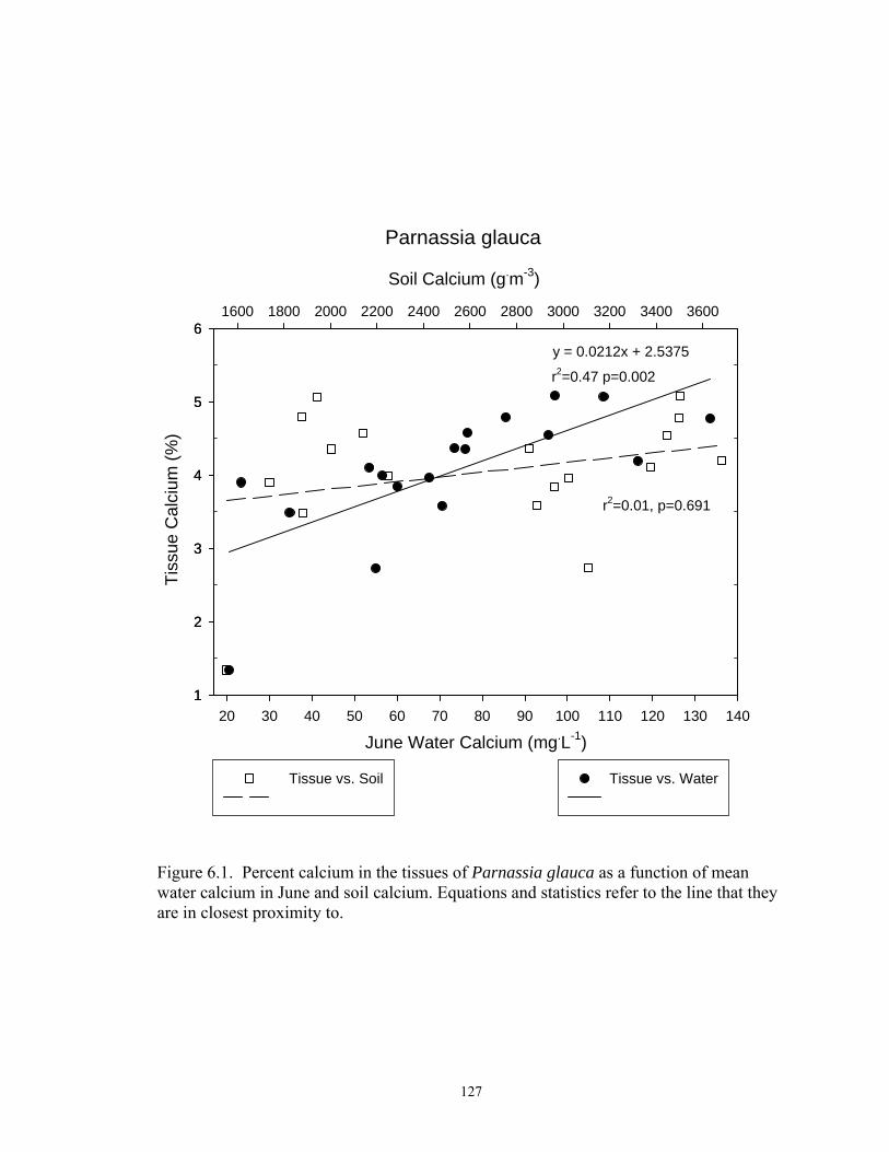
127

Parnassia glauca

Soil Calcium (g.m-3)

1600 1800 2000 2200 2400 2600 2800 3000 3200 3400 3600

1

2

3

4

5

6

Tissue vs. Soil

June Water Calcium (mg.L-1)20 30 40 50 60 70 80 90 100 110 120 130 140

Tiss

ue C

alci

um (%

)

1

2

3

4

5

6

Tissue vs. Water

y = 0.0212x + 2.5375

r2=0.47 p=0.002

r2=0.01, p=0.691

Figure 6.1. Percent calcium in the tissues of Parnassia glauca as a function of mean water calcium in June and soil calcium. Equations and statistics refer to the line that they are in closest proximity to.

128

calcium at all months when water calcium was measured, although these comparisons

may not be very meaningful. This species is the only one for which the best-fit curve was

non-linear (Figure 6.2). The tissue concentration appeared to reach an asymptote once it

reached about 4.5%. The tissue concentration increased linearly as water calcium did

until it reached a critical concentration around 80mg.L-1. At this point, there was little

change in tissue concentrations as water calcium levels continued to increase. It appears

that this species reached a "saturation" level of environmental calcium and tissue calcium

only increased very slightly as environmental levels did. This result is not surprising

considering that the actual percent of calcium in its tissues already exceeds that of most

dicots. Thus, this species does exclude calcium from its tissues; however, only after it

has accumulated more than most plants would.

129

Parnassia glauca


1600 1800 2000 2200 2400 2600 2800 3000 3200 3400 3600

1

2

3

4

5

6

Tissue vs. Soil

0 10 20 30 40 50 60 70 80 90 100 110 120 130 1401

2

3

4

5

6

Tissue vs. Water

Tiss

ue C

alci

um (%

)

June Water Calcium (mg.L-1)

y = 2.113*(1-x(-0.0558x))R2 = 0.538, p=0.0005

Figure 6.2. Best fit line (exponential rise, single, 2 parameter) for relationship between percent calcium in the tissues of Parnassia glauca as a function of mean water calcium in June and soil calcium. Equations and statistics refer to the line that they are in closest proximity to.

Calcium in the tissues of Equisetum fluviatile showed a significant correlation to the

water calcium in June (r2=0.40 p=0.036; Figure 6.3) and did not show a significant

correlation with the soil calcium (r2=0.02, p=0.700). Symphyotrichum puniceum and

Packera aurea showed significant correlations of tissue calcium to the water calcium in

months proceeding their collection in May and June. Calcium in the tissues of

130

Symphyotrichum puniceum was correlated to the water calcium in May (r2=0.23,

p=0.047; not shown) slightly less strongly than it was to June water calcium (r2=0.27,

p=0.027; Figure 6.4) and was not correlated to soil calcium (r2=0.05 p=0.393; Figure

6.4).

Equisetum fluviatile

Soil Calcium (g.m -3)

2000 2200 2400 2600 2800 3000 3200 3400 3600 3800

1.5

1.6

1.7

1.8

1.9

2.0

2.1

2.2

2.3

Tissue vs. Soil

r2=0.40 p=0.036

r2=0.02, p=0.700

y = 0.0042x + 1.5869

June Water Calcium (mg.L-1)30 40 50 60 70 80 90 100 110 120 130 140

Tiss

ue C

alci

um (%

)

1.5

1.6

1.7

1.8

1.9

2.0

2.1

2.2

2.3

Tissue vs. Water

Figure 6.3. Percent calcium in the tissues of Equisetum fluviatile as compared to mean water calcium in June and soil calcium. Equations and statistics refer to the line that they are in closest proximity to.

131

Symphyotrichum puniceum


1800 2000 2200 2400 2600 2800 3000 3200 3400 3600 3800

0.6

0.8

1.0

1.2

1.4

1.6

Tissue vs. Soil

r2=0.05 p=0.393

y = 0.0044x + 0.6856r2=0.27, p=0.027


Tiss

ue C

alci

um (%

)

0.6

0.8

1.0

1.2

1.4

1.6

Tissue vs. Water

Figure 6.4. Percent calcium in the tissues of Symphyotrichum puniceum as compared to mean water calcium in June and soil calcium. Equations and statistics refer to the line that they are in closest proximity to.

Tissue calcium of Packera aurea was correlated to the water calcium in May (r2=0.50,

p=0.016; not shown) somewhat stronger than it was in June (r2=0.41, p=0.034; Figure

6.5) and exhibited an almost identical trend in June as it did with soil calcium (r2=0.57,

p=0.007; Figure 6.5). It is interesting that Packera aurea is correlated to soil and water

calcium, as no other species showed this relationship. Perhaps this response suggests that

in sites where this species occurred, the soil and water calcium were correlated with each

132

other. This correlation would exist if Packera aurea was only found at sites that had

steady inputs of groundwater and fairly unchanging calcium levels. Upon further

inspection, no relationship was detected as this species occurred at sites where calcium

remained fairly constant (e.g., Shmulsky Shrub) and where large differences were

observed (e.g. Shmulsky Open). Thus, the relationship between the tissue calcium of this

species to both environmental calcium forms (in May, and June) remains unexplained.

Packera aurea


1600 1800 2000 2200 2400 2600 2800 3000 3200 3400 3600 3800

1.0

1.2

1.4

1.6

1.8

2.0

2.2

Tissue vs. Soil

y = 0.0003x + 0.614

r2=0.41, p=0.034y = 0.0064x + 0.9821

r2=0.57, p=0.007


Tiss

ue C

alci

um (%

)

1.0

1.2

1.4

1.6

1.8

2.0

2.2

Tissue vs. Water

Figure 6.5. Percent calcium in the tissues of Packera aurea as compared to mean water calcium in June and soil calcium. Equations and statistics refer to the line that they are in closest proximity to.

133

The calcium in the tissues of Symplocarpus foetidus was not correlated significantly

with water calcium (for June r2=0.0273 p=0.589) but showed a significant relationship to

the soil calcium (r2=0.33, p=0.040; Figure 6.6). This species is the only one that

correlates solely to the soil calcium. This correlation may be related to the fact that this

Symplocarpus foetidus


1600 1800 2000 2200 2400 2600 2800 3000 3200 3400 3600 3800

1.4

1.6

1.8

2.0

2.2

2.4

2.6

2.8

3.0

3.2

3.4

Tissue vs. Soil

r2=0.0273 p=0.589

r2=0.33, p=0.040

y = 0.0004x + 0.9062

June Water Calcium (mg.L-1)20 30 40 50 60 70 80 90 100 110 120

Tiss

ue C

alci

um (%

)

1.4

1.6

1.8

2.0

2.2

2.4

2.6

2.8

3.0

3.2

3.4

Tissue vs. Water

Figure 6.6. Percent calcium in the tissues of Symplocarpus foetidus as compared to mean water calcium in June and soil calcium. Equations and statistics refer to the line that they are in closest proximity to.

134

species has the ability to uncouple electron transport and ATP production and release

energy as heat (Solomon et al., 1996). This gives this species the ability to begin growth

early in the spring when snow is still on the ground. Even though the leaves collected for

analysis were the most recently mature leaves, this process may have resulted in their

development far earlier in the season than the other species sampled. Thus, water

measurements taken may not have been reflective of the growing conditions when the

leaves formed. The soil calcium could more accurately reflect the average pool of

available calcium released into the system and thus reflect this earlier period of uptake.

No significant correlations were observed between tissue and soil/water calcium for

Carex flava, Carex hystericina, Dasiphora fruticosa, Eriophorum viridicarinatum,

Fragaria vesca, Mentha arvensis, Solidago patula, and Thelypteris palustris (Table 6.2).

Table 6.2. Statistics for species with no correlation between tissue calcium and soil and mean water calcium in June.

Species water soil r2 p r2 p

Carex flava 0.044 0.434 0.059 0.365

Carex hystericina 0.196 0.200 0.013 0.756

Dasiphora fruticosa 0.060 0.272 0.0002 0.950

Eriophorum viridicarinatum 0.038 0.616 0.084 0.449

Fragaria vesca 0.038 0.591 0.192 0.205

Mentha arvensis 0.176 0.154 0.002 0.888

Solidago patula 0.002 0.895 0.014 0.715

Thelypteris palustris 0.004 0.793 0.049 0.350

135

Summary

Parnassia glauca, Equisetum fluviatile, Symphyotrichum puniceum, Dasiphora

fruticosa and Packera aurea are recognized as calciphiles in the literature as discussed in

Chapter 4, but of these only Parnassia glauca and Packera aurea were shown in Chapter

5 to respond in distribution and abundance to environmental calcium levels. All of these

species except Dasiphora fruticosa, do however, display a significant correlation between

levels of calcium in their tissues and calcium in the environment.

The occurrence of Equisetum fluviatile and Symphyotrichum puniceum in calcareous

fens indicates that these plants are obviously tolerant of elevated calcium levels even

though they may not need those high levels for increased growth or health. Since they

are accumulating this element, they must have a mechanism for keeping it from affecting

vital processes.

It was interesting to observe that neither Dasiphora fruticosa, Carex flava, nor Carex

hystericina showed correlations in calcium accumulation to calcium availability since

these species were originally deemed calciphiles in Chapter 4. This study, however,

showed that although these three species were present in calcareous environments, their

distribution and abundance did not change in relation to variations in environmental

calcium levels. Thus, these species may be excluding calcium actively from their tissues

beyond a certain point of accumulation. Perhaps, these plants are found once a slightly

higher level of calcium exists, as compared to 'non-calciphiles', which is why they occur

where they do. Thus, all of the sites in this study may have exceeded the minimum

calcium threshold for these species. In addition, abundance of Dasiphora fruticosa was

determined in Chapter 5 to be correlated strongly with gradients in pH, more so than

136

calcium, and thus it makes sense for this species to exclude calcium if pH affects its

distribution most.

Similar calcium-independent relationships can be concluded for the species that also

had no abundance changes in relation to calcium as determined in Chapter 5, i.e., Mentha

arvensis, Solidago patula, Eriophorum viridicarinatum, Thelypteris palustris, and

Fragaria vesca. This finding is consistent with the generalist nature of Thelypteris

palustris, but presents an interesting situation for Solidago patula and Eriophorum

viridicarinatum who appeared to be calciphiles from early literature reports. These

findings suggest that these species have a weak relationship with calcium, even though

they are found mostly in calcareous environments.

It was very curious to observe that both Mentha arvensis and Symplocarpus foetidus,

common wetland species, showed substantial levels of calcium accumulation that

correlated with water or soil calcium levels. The precipitation of calcium oxalate crystals

has been observed in species in the Lamiaceae (as is Mentha arvensis) (Kinzel, 1983) and

in Symplocarpus foetidus (Higley, 1880) and this process may relate to why these plants

can absorb large quantities of calcium. This action does not mean that these species are

calciphiles as they exist in areas without high calcium levels but suggests that their needs

for calcium are low and that they can grow in environments where calcium is elevated as

they have a successful mechanism by which to tolerate it.

Magnesium

Plants absorbed 0.1 to 0.9 % magnesium into their tissues; however, the average was

less than 0.5%. Parnassia glauca had the greatest average tissue magnesium at 0.7%

(Table 6.3). Only two species, Thelypteris palustris and Carex flava, showed significant

137

correlations between the magnesium in their tissues to the magnesium in the water or

soil. Tissue magnesium in Thelypteris palustris had a highly significant correlation to the

water magnesium in June (the month proceeding its leaf collection) (r2=0.73 p=0.007)

(Figure 6.7). Carex flava (Figure 6.8) had a significant correlation with the water

magnesium for all months proceeding and during its collection, and thus the water

magnesium for June is reported (r2=0.75 p=0.012). In addition, this species showed a

very strong correlation to the soil magnesium as well (r2=0.77, p=0.009).

Table 6.3. Mean percent magnesium and percent magnesium range in the tissues of the thirteen species collected from the eight study sites. Means are presented ± standard deviation. Means with different letters are significantly different by Tukey’s Test (p=0.05). Composite samples (n) = number of plots where that species occurred. Number of sites where these samples were collected are included for reference.

Species Code % Magnesium % Magnesium Range

Composite samples Sites

Parnassia glauca 0.7 ± 0.1 a 0.5 – 0.9 8 6

Mentha arvensis 0.6 ± 0.3 ab 0.2 – 1.2 8 6

Packera aurea 0.4 ± 0.1 abc 0.3 – 0.6 5 5

Equisetum fluviatile 0.4 ± 0.04 abc 0.4 – 0.5 5 4

Symplocarpus foetidus 0.4 ± 0.1 abcd 0.4 – 0.6 4 4

Solidago patula 0.3 ± 0.1 bcd 0.2 – 0.4 5 4

Thelypteris palustris 0.3 ± 0.1 cd 0.3 – 0.5 8 8

Dasiphora fruticosa 0.3 ± 0.03 cd 0.2 – 0.3 6 6

Carex flava 0.3 ± 0.1 cd 0.2 – 0.4 7 7

Fragaria vesca 0.3 ± 0.1 cd 0.1 – 0.5 6 6 Symphyotrichum puniceum 0.2 ± 0.1 cde 0.1 – 0.4 9 6 Carex hystericina 0.2 ± 0.1 cde 0.1 – 0.4 7 6

Eriophorum viridicarinatum 0.1 ± 0.1 de 0.1 – 0.2 7 5

Carex granularis 0.09 ± 0.1 de 0.0 - 0.18 2 2

138

Thelypteris palustris

Soil Magnesium (g.m-3)

200 250 300 350 400 450 500

0.20

0.25

0.30

0.35

0.40

0.45

0.50

Tissue vs. Soil

y = 0.004x + 0.1773

r2=0.37, p=0.110

r2=0.73 p=0.007

June Water Magnesium (mg.L-1)15 20 25 30 35 40 45 50 55 60 65 70

Tiss

ue M

agne

sium

(%)

0.20

0.25

0.30

0.35

0.40

0.45

0.50

Tissue vs. Water

Figure 6.7. Percent magnesium in the tissues of Thelypteris palustris as compared to mean water magnesium in June and soil magnesium. Equations and statistics refer to the line that they are in closest proximity to.

139

Carex flava

Soil Magnesium (g.m-3)

250 300 350 400 450 500 550

0.15

0.20

0.25

0.30

0.35

0.40

0.45

Tissue vs. Soil

y = 0.0005x + 0.0991

y = 0.0031x + 0.1853r2=0.75 p=0.012

r2=0.77, p=0.009

June Water Magnesium (mg.L-1)10 15 20 25 30 35 40 45 50 55 60 65

Tiss

ue M

agne

sium

(%)

0.15

0.20

0.25

0.30

0.35

0.40

0.45

Tissue vs. Water

Figure 6.8. Percent magnesium in the tissues of Carex flava as compared to mean water magnesium in June and soil magnesium. Equations and statistics refer to the line that they are in closest proximity to.

Carex flava and Thelypteris palustris present interesting comparisons to the species

that responded physiologically to environmental calcium. Carex flava was considered to

be a calciphile, but appeared to restrict calcium accumulation in its tissues. This response

was interesting since this species did not appear to increase in abundance in response to

environmental calcium as described in Chapter 5. This accumulation of magnesium in

140

relation to the available supply would seem to suggest that the environmental magnesium

concentration, rather than calcium, is somehow important to the growth of this species.

Perhaps this species is considered to be a calciphile because it occurs in calcium-enriched

areas, but in actuality is selecting calcareous fen habitats for the elevated magnesium

levels associated with them. This may particularly be where dolomitic limestone

dominates.

Thelypteris palustris, which was considered to be a common wetland fern, exhibited a

strong relationship to the magnesium it absorbs in relation to water magnesium levels

(Figure 6.7). This activity is particularly interesting as it did not absorb calcium in

proportion to the available calcium supply. The reasons as to why this species would

accumulate greater of amounts of magnesium into its tissues is unknown; however, the

accumulation may be associated with either a need for or tolerance to magnesium,

explaining why it is also common in calcareous fens.

Magnesium is essential for plants as it is the central atom of the chlorophyll molecule

(Walker and Weinstien, 1991) and is involved in regulation of cellular pH and ionic

balance (Marschner, 1995) among other processes. The accumulation of magnesium in

the current study was higher than the amount of magnesium generally required by plants

(0.15 - 0.35%; Marschner, 1995) and is indicative of an abundant supply (Marschner,

1995). It is interesting that Thelypteris palustris and Carex flava did not have the highest

levels of tissue magnesium in this study even as they appeared to accumulate more

magnesium as more was available. Interestingly, the other calciphiles had higher tissue

magnesium levels than these species but did not exhibit continuously enhanced

accumulation as the supply increased.

141

Since in calcareous fens, water calcium and water magnesium often are correlated

closely (Chapter 3), changes in plant distributions associated with calcium could just as

easily be related to magnesium. Although similar plant communities often occur in

nondolomitic-influenced fens, these results convey the importance of calcium to the

calciphiles. At most of the sites, calcium and magnesium absorption was competitive as

values exceeded 0.001M (Marschner, 1995). All of the species that showed significant

tissue-environmental calcium correlations did not show the same relationship to

magnesium. This finding indicates that while the calciphiles selectively allowed calcium

into their tissues, they actively excluded magnesium. Thus the magnesium supply

appears to be less important for most calciphiles as compared to the calcium supply. By

contrast, Carex flava (a calciphile) and Thelypteris palustris (a generalist), may have a

greater physiological need for magnesium, which explains their increased uptake of it (to

the exclusion of calcium) and details possible reasons that they are found in calcareous

fens.

Literature Revisited

In general, species tissue calcium fell within the expected range of 0.1% – 5.0% dry

weight (White and Broadley, 2003), and Parnassia glauca showed the highest levels and

most remarkable changes in accumulation as water concentrations increased. Monocots

had generally lower values (<1%) than dicots (>1%). The general conclusions of this

study validate the findings of Clarkson (1965), who reported that calciphiles absorb

calcium in larger amounts than non-calciphiles. It is interesting however that not all

species originally suspected to be calciphiles showed this relationship. All of the species

that showed a response to environmental calcium in their abundance did show increased

142

levels of calcium in their tissues in response to increased calcium in the environment.

However, it appears that among species for which abundance was not affected by

environmental calcium levels, some restrict its absorption and some do not.

It is difficult to compare the results of the exact concentrations of calcium and

magnesium in the plants studied with previous research since for many of these species

these data have never been reported. For Dasiphora fruticosa, however, Marosz (2004)

measured the accumulation of calcium and other elements along an experimental soil

salinity gradient. He reported that calcium values in leaves varied between 0.71 and 0.89

% dry weight in a solution that had an undisclosed amount of calcium in it. The calcium

concentration of the leaves of Dasiphora fruticosa analyzed in this study were higher (1.0

- 1.6 %). This result may indicate that in calcareous fens, the substrate calcium levels are

elevated beyond the minimum threshold required for this species. Thus, the plants may

have higher average tissue concentrations, but that accumulation is not related to

environmental levels. Another explanation for why the values were lower in Marosz’s

study could be that he studied a different variety of Dasiphora fruticosa in which its

calcium uptake differed from the native North American varieties. Marosz observed

changes in the accumulation of calcium in the tissues, but this response was related to

increased soil salinity. It was proposed that this response had to do with the changes in

osmotic potential as a result of increased sodium chloride (NaCl); however, other

research has indicated that the uptake of calcium decreases when NaCl concentrations are

high (Lynch and Lauchli, 1985) as the NaCl might inhibit calcium transport from the

external medium into the root xylem under certain circumstances.

Previous research on the calcium accumulation in Geum rivale had reported that it had

143

3.4 % calcium in its leaves (Waldren et al., 1987). Although the value measured the

current study was higher than many of the dicots (1.9%), it was not nearly as high as

observed by Waldren et al. (1987). Since this species occurred only at an elevated

calcium threshold, a very strong relationship may exist between its tissue calcium and

environmental calcium. Since only one sample was collected and analyzed for calcium,

relationships to the environment were not established, and if perhaps, this one sample

was collected where environmental levels were lower than in the current study, its tissue

level may also be lower. Waldren et al. (1987) does not report the substrate calcium

conditions for comparison.

Auclair (1979) found that Equisetum fluviatile had elevated concentrations of iron and

calcium in its tissues as compared to other elements. Calcium values measured 1.8%;

however, the water calcium and iron were not measured. This value corresponds to the

mean tissue calcium of Equisetum fluviatile measured in this study (1.9%). This high

accumulation of calcium (in addition to iron as mentioned in Chapter 5) indicates the

strong ability for this species to sequester ions in general and that this species has a

unique response to calcium and iron in the environment.

Conclusions

Although this study has not analyzed how calcium is used in plants of calcareous fens,

it has established that five species common to calcareous fens (Parnassia glauca,

Packera aurea, Symphyotrichum puniceum, Equisetum fluviatile, and Symplocarpus

foetidus) accumulate calcium in response to amounts available in their environment. It is

evident that these species grow well in calcareous environments because they are either

protected from the toxicity of excess calcium, or they actually need the calcium for

144

various aspects of their growth and development. In addition, not all plants maintain the

same levels of calcium in their tissues, and there are large differences among species.

The most important finding in relation to these trends is the confirmation that the species

that showed the strongest correlation of their tissue calcium to environmental calcium

levels are species that are associated with calcareous environments. Some of these

species showed changes in distribution and abundance with changes in environmental

calcium (Parnassia glauca, Packera aurea), and some did not (Symphyotrichum

puniceum and Equisetum fluviatile). On the contrary, most of the non-calciphiles were

restrictive in the amount of calcium they accumulated and maintained steady levels as

calcium supply increased. Species originally deemed calciphiles (based on the literature)

such as Dasiphora fruticosa, Carex hystericina, and Carex flava did not show a

significant relationship between their tissue calcium and environmental calcium levels,

and this observation may be related to the lack of relationship between environmental

calcium and their abundance as was previously determined in Chapter 5. The subsample

analysis of tissue magnesium highlighted the relationship of Carex flava and Thelypteris

palustris to environmental magnesium levels as their tissue magnesium was correlated to

the environmental magnesium levels and not to the calcium supply.

145

CHAPTER VII

CONCLUSIONS

This study has reinforced current knowledge that calcareous fens are unique and

fascinating ecosystems. Although these wetlands exhibit the quality of being enriched

with calcium, the degree to which it accumulates in plants varies widely. In addition,

processes bringing groundwater to the surface are not necessarily similar among fens in

close proximity to each other, as site geochemistry showed significant variation. As a

result, patterns of species distribution vary among and within fen ecosystems. This thesis

identified individual species for which distributions and physiological responses appear

to be linked strongly to the chemical properties of calcareous fens. However, some

original hypotheses on the relationships between specific plants and the chemical factors

were rejected: some calciphiles did not appear to show any response to environmental

calcium other than being tolerant to elevated levels. The following section will revisit the

original hypotheses and reevaluate them based on the new knowledge of plant selectivity

in calcareous fens.

Hypotheses Revisited

The original hypotheses suggested that:

1) Specific environmental substrate calcium levels can be identified and a minimum

and maximum range can be established for each calciphile as well as a threshold

of calcium that must be met for a given species to occur.

This study successfully monitored the chemical and hydrologic environment of eight

calcareous fens in the Berkshire-Taconic region of Western Massachusetts over the

course of one growing season. Sites varied greatly in their soil and water calcium levels,

146

and for some species, these differences appeared to influence their abundance. For

species that occurred only above a specific calcium threshold, that level was noted.

Likewise, for species for which abundance appeared to increase as environmental levels

did, that range was noted. Although these values may not represent all absolute

possibilities as to the geochemical environment in which these species occur, they

provide an estimate (based on 24 sampling locations) as to the environmental calcium

selectivity of these species as this had not been accomplished previously. Future research

should expand the number of study sites and focus on these particular species to try to

determine if this trend holds in general or across different climate regimes.

2) The most selective calciphile species (calcium specialists) that grow in calcareous

fens will have the highest calcium concentrations in their tissues and these levels

will correspond to environmental substrate calcium levels.

The species that appeared to be most responsive to environmental calcium levels were

Parnassia glauca, Geum rivale, Carex sterilis, Carex granularis, Carex leptalea, and

Packera aurea (the threshold and gradient species). Of these, calcium tissue

concentrations in Parnassia glauca and Packera aurea were compared to environmental

calcium levels. Both of these species showed significantly higher accumulation of

calcium as environmental levels increased indicating that these species do not selectively

exclude calcium from their tissues.

Although several non-calciphile species had calcium tissue concentrations greater than

Packera aurea, Parnassia glauca had unusually high levels, at times above 5%. Analysis

of Geum rivale and Carex granularis showed that they too had elevated calcium levels

compared to the non-calciphiles, particularly Carex granularis, which had the highest

147

concentration of the monocots. It appears that in general, plants that increase in

abundance in relation to environmental calcium levels also have high concentrations of

calcium in their tissues. In addition, these tissue levels increase as environmental levels

increase; indicating that these plants’ adaptations are extremely efficient at facilitating

growth in calcareous environments.

3) The least selective species (calcium generalists) that grow in calcareous fens will

maintain lower tissue calcium levels that will appear to be absorbed independent

of environmental substrate levels.

The calcium generalists were determined to be Carex flava, Carex hystericina,

Equisetum fluviatile, Juncus nodosus, Solidago patula, Solidago uliginosa,

Symphyotrichum puniceum, Symplocarpus foetidus, Thelypteris palustris, Dasiphora

fruticosa, and Juncus brachycephalus. Of these, tissue analyses were conducted on

Symphyotrichum puniceum, Symplocarpus foetidus, Thelypteris palustris, Dasiphora

fruticosa, Solidago patula, Carex flava, Carex hystericina, and Equisetum fluviatile.

Most of these species did not show a significant relationship between the amount of

calcium in their tissues and the environmental calcium levels; however, Symphyotrichum

puniceum, Equisetum fluviatile and Symplocarpus foetidus did. Even more fascinating is

that two of these species (Symplocarpus foetidus and Equisetum fluviatile) had the third

and fourth (respectively) highest calcium in their tissues. Therefore, it does not appear

that all generalists exclude calcium as environmental levels increase.

148

Modes of Growth in Calcareous Fens

In conclusion, there appear to be several factors that regulate a plant’s occurrence and

growth in a calcareous environment.

1) Certain plant species increase in abundance as calcium does and have elevated

levels of tissue calcium that increase as environmental levels do. These plants are

ecological calciphiles but without knowledge of the amount of water soluble calcium in

their tissues, it cannot be said whether they are also physiological calciphiles.

Nevertheless, these species have strong adaptations to dealing with large amounts of

calcium in their systems and to the other limitations associated with calcium-rich

environments. Although speculative, these plants may have a physiological need for

calcium that is satisfied when they grow in a calcareous fen. These plants can be said to

be calciphile specialists and include Parnassia glauca, Packera aurea, Geum rivale,

Carex granularis and possibly Carex leptalea.

2) Certain calciphiles do not increase in abundance relative to environmental calcium

levels and exclude calcium from their tissues. These plants are thus tolerant of elevated

calcium levels and are perhaps better competitors in those environments because they

have well-suited mechanisms to avoid the toxicity that calcium can impose and/or benefit

from non-calcium related aspects of fen geochemistry. The distribution of these species

cannot be linked directly to environmental calcium levels. Thus, plants of this sort may

have more than one physiological response to dealing with the excess calcium. It is

likely that they either A) exclude the calcium from their tissues and maintain constantly

lower levels, or they B) have an ability to absorb higher calcium levels without it

affecting physiological processes. Condition A) is represented by species, such as Carex

149

hystericina, Eriophorum viridicarinatum, and Solidago patula, which exhibited no

relationship to environmental calcium other than growing in elevated levels of it.

Condition B) is represented by Symphyotrichum puniceum, Equisetum fluviatile and

Symplocarpus foetidus, which all had higher concentrations of calcium and accumulated

calcium in greater amounts as environmental calcium levels increased. Both of these

conditions could include a third response, in which growth in a calcareous fen appears to

be associated with accessory benefits such as elevated pH or increased magnesium levels.

Species that appeared to fall into this growth regime were Dasiphora fruticosa and

Juncus brachycephalus, which appeared to respond to pH gradients and Carex flava and

Thelypteris palustris, which may have a physiological response to magnesium. For

species of this sort that are ecological calciphiles, it can be said that they are calciphile

generalists. However, while behaving as calcium generalists, Thelypteris palustris and

Symplocarpus foetidus would not be considered ecological calciphiles due to their

occurrence elsewhere.

Future Research

This project has analyzed many new and interesting aspects of plant relationships and

environmental substrate gradients in calcareous fens. However these new answers have

fueled new questions. The following section will list research that needs to be considered

in this area to strengthen the investigations presented in this thesis.

1) The current study could be expanded to determine if the same species-

environmental gradient relationships hold true for a larger geographic or climatic region.

Investigations of the responses of Juncus brachycephalus and Dasiphora fruticosa to pH

gradients are needed to verify and explain them. The response of Equisetum fluviatile to

150

an iron gradient instead of a calcium gradient needs further study. Whether Geum rivale,

Carex sterilis and Carex granularis ever occur below the calcium threshold established in

this study needs further verification as does whether Parnassia glauca and Packera aurea

continue to show distribution increases as environmental calcium increases.

2) A similar study as to this one could be repeated in which more leaf samples of

Geum rivale, Carex granularis and Carex leptalea are collected from multiple sites and

analyzed for calcium. Currently it is still not clear whether these three species absorb

calcium in proportion to environmental availability.

Overall, only subsets of the plants collected were analyzed for tissue magnesium. A

similar study should be conducted in which the tissues of a suite of species growing

across an environmental magnesium gradient are analyzed for magnesium and compared

to the environmental levels. It would be important to focus on Carex flava and

Thelypteris palustris, as they showed very strong correlations to the magnesium supply in

the current study. In addition, sites where Carex flava occurs across the country should

be compared with geologic information to see if its distribution relates to calcareous fens

that are fed by groundwater that has passed through dolomite limestone and would thus

have a significant magnesium input.

No rare species were analyzed in this study and thus it would be interesting to see if

the tissues of some of the endangered and threatened species of calcareous fens also

absorb elevated levels of calcium.

3) Although perhaps a difficult question to answer, it would be interesting to

understand what plants in calcareous fens do with the extra calcium that they absorb.

This would include an analysis of the forms of calcium that it is stored in and where it is

151

stored. If calcium in the tissues of the ecological calciphiles is soluble as calcium malate,

then these species would also be physiological calciphiles. It would be interesting to

determine which species, if any, are of this nature. In addition, it is still unclear if the

ecological calciphiles need more calcium and if so, for what purpose. For the generalists

species (and physiological calcifuges), it would be interesting to understand the dominant

forms that calcium is stored in and/or how they may exclude it.

4) All study sites shared typical characteristics of calcareous fens. They all had

elevated calcium levels, elevated pH, extended periods of saturation, and plant

communities that included many calciphiles. There were, however, large differences in

all of these characteristics among sites, even among those that were adjacent. It would be

interesting to understand the sources and reasons of this variability and provide more

detailed characterizations of the hydrogeochemical settings. This investigation would

involve tracking groundwater movement and determining the specific bedrock types to

which upwelling groundwater in each site was exposed and how known atomic ratios of

elements in the surrounding bedrock relate to those measured in the sites. It will be

important to determine the proximity of the point of delivery of groundwater to the site

and verify whether sites are supplied direct upwelling groundwater or how long that

water may have traveled through the soil as subsurface flow. In addition, it will be

important to monitor if the waters are diluted by other sources (i.e. nearby streams or

non-calcareous groundwater flow paths) and how these and other factors may influence

the pore-water geochemistry.

152

APPENDICES

153

APPENDIX A

STOCKBRIDGE FORMATION

154

Figure A.1. The Stockbridge Formation (Zen and Ratcliffe, 1971)

155

APPENDIX B

SITE PHOTOS

156

156

Figure B.1. Vegetation community at Jug End North.

157

157

Figure B.2. Vegetation community and water monitoring instruments at Jug End South.

158

158

a)

b)

Figure B.3. General vegetation at of Schenob Brook Bartholomew: a) plot SBB3, b) adjacent agricultural fields.

159

159

Figure B.4. General view of vegetation at Schenob Brook North.

160

160

a)

c)

b)

Figure B.5. Unique species at Schenob Brook North: a) Pogonia ophioglossoides, b) Calopogon tuberosus, c) Spiranthes cernua.

161

161

Figure B.6. Vegetation community at Schenob Brook Central in autumn of 2006.

162

162

Figure B.7. Hummock landscape at Schenob Brook South before the emergence of vegetation in March, 2006.

163

163

a)

b)

Figure B.8. Vegetation at Shmulsky Open: a) general fen view, and b) plant composition and sampling well at SO1.

164

164

Figure B.9. Vegetation cover at Shmulsky Shrub, plot 1.

165

165

APPENDIX C

QUALITATIVE ASSESSMENT OF REDUCED IRON

166

Figure C.1. Reduced iron at Jug End North (JN).

Figure C.2. Reduced iron at Jug End South (JS).

May 18

June

10

June

19Ju

ly 6

July

17Aug

ust 1

Augus

t 15

Sept. 7

Sept

. 21

Oct. 18

Oct. 5

Reduced Iron (Fe2+) – Jug End North

0-15

15-30

Depth (cm)

= none = low = high= medium = no data

May 18

June

10

June

19Ju

ly 6

July

17Aug

ust 1

Augus

t 15

Sept. 7

Sept

. 21

Oct. 18

Oct. 5

Reduced Iron (Fe2+) – Jug End North

0-15

15-30

Depth (cm)


May 18

June

10

June

19Ju

ly 6

July

17Aug

ust 1

Augus

t 15

Sept. 7

Sept

. 21

Oct. 18

Oct. 5

Reduced Iron (Fe2+) – Jug End South

0-15

15-30

Depth (cm)


May 18

June

10

June

19Ju

ly 6

July

17Aug

ust 1

Augus

t 15

Sept. 7

Sept

. 21

Oct. 18

Oct. 5

Reduced Iron (Fe2+) – Jug End South

0-15

15-30

Depth (cm)


167

Figure C.3. Reduced iron at Bartholomew (SBB).

Figure C.4. Reduced iron at Schenob Brook Central (SBC).

May 18

June

10

June

19Ju

ly 6

July

17Aug

ust 1

Augus

t 15

Sept. 7

Sept

. 21

Oct. 18

Oct. 5

Reduced Iron (Fe2+) - Bartholomew

0-15

15-30

Depth (cm)


May 18

June

10

June

19Ju

ly 6

July

17Aug

ust 1

Augus

t 15

Sept. 7

Sept

. 21

Oct. 18

Oct. 5

Reduced Iron (Fe2+) - Bartholomew

0-15

15-30

Depth (cm)


May 18

June

10

June

19Ju

ly 6

July

17Aug

ust 1

Augus

t 15

Sept. 7

Sept

. 21

Oct. 18

Oct. 5

Reduced Iron (Fe2+) – Schenob Brook Central

0-15

15-30

Depth (cm)


May 18

June

10

June

19Ju

ly 6

July

17Aug

ust 1

Augus

t 15

Sept. 7

Sept

. 21

Oct. 18

Oct. 5

Reduced Iron (Fe2+) – Schenob Brook Central

0-15

15-30

Depth (cm)


168

Figure C.5. Reduced iron at Schenob Brook North (SBN)

Figure C.6. Reduced iron at Schenob Brook South (SBS).

May 18

June

10

June

19Ju

ly 6

July

17Aug

ust 1

Augus

t 15

Sept. 7

Sept

. 21

Oct. 18

Oct. 5

Reduced Iron (Fe2+) – Schenob Brook North

0-15

15-30

Depth (cm)


May 18

June

10

June

19Ju

ly 6

July

17Aug

ust 1

Augus

t 15

Sept. 7

Sept

. 21

Oct. 18

Oct. 5

Reduced Iron (Fe2+) – Schenob Brook North

0-15

15-30

Depth (cm)


May 18

June

10

June

19Ju

ly 6

July

17Aug

ust 1

Augus

t 15

Sept. 7

Sept

. 21

Oct. 18

Oct. 5

Reduced Iron (Fe2+) – Schenob Brook South

0-15

15-30

Depth (cm)


May 18

June

10

June

19Ju

ly 6

July

17Aug

ust 1

Augus

t 15

Sept. 7

Sept

. 21

Oct. 18

Oct. 5

Reduced Iron (Fe2+) – Schenob Brook South

0-15

15-30

Depth (cm)


169

Figure C.7. Reduced iron at Shmulsky Open (SO)

Figure C.8. Reduced iron at Shmulsky Shrub (SS)

May 18

June

10

June

19Ju

ly 6

July

17Aug

ust 1

Augus

t 15

Sept. 7

Sept

. 21

Oct. 18

Oct. 5

Reduced Iron (Fe2+) – Shmulsky Open

0-15

15-30

Depth (cm)


May 18

June

10

June

19Ju

ly 6

July

17Aug

ust 1

Augus

t 15

Sept. 7

Sept

. 21

Oct. 18

Oct. 5

Reduced Iron (Fe2+) – Shmulsky Open

0-15

15-30

Depth (cm)


May 18

June

10

June

19Ju

ly 6

July

17Aug

ust 1

Augus

t 15

Sept. 7

Sept

. 21

Oct. 18

Oct. 5

Reduced Iron (Fe2+) – Shmulsky Shrub

0-15

15-30

Depth (cm)


May 18

June

10

June

19Ju

ly 6

July

17Aug

ust 1

Augus

t 15

Sept. 7

Sept

. 21

Oct. 18

Oct. 5

Reduced Iron (Fe2+) – Shmulsky Shrub

0-15

15-30

Depth (cm)


170

APPENDIX D

SEASONAL VARIATION IN PH

171

Shmulsky - Water pH

2006

May 4

May 18

June

10

June

19Ju

ly 6

July

17

Augus

t 1

Augus

t 15

Sept. 7

Sept. 2

1Oct.

5

Oct. 18

pH

6.4

6.6

6.8

7.0

7.2

7.4

7.6Shmulsky OpenShmulsky Shrub

Figure D.1. Seasonal variation in water pH at the two sites in the Shmulsky location. Each point represents a mean of three replicate samples.

Schenob Brook - Water pH

2006

May 4

May 18

June

10

June

19Ju

ly 6

July

17

Augus

t 1

Augus

t 15

Sept. 7

Sept. 2

1Oct.

5

Oct. 18

pH

6.4

6.6

6.8

7.0

7.2

7.4

7.6BartholomewSchenob CentralSchenob NorthSchenob South

Figure D.2. Seasonal variation in water pH at the four sites in the Schenob Brook location. Each point represents a mean of three replicate samples.

172

Jug End - Water pH

2006

May 4

May 18

June

10

June

19Ju

ly 6

July

17

Augus

t 1

Augus

t 15

Sept. 7

Sept. 2

1Oct.

5

Oct. 18

pH

6.4

6.6

6.8

7.0

7.2

7.4

7.6

Jug End NorthJug End South

Figure D.3. Seasonal variation in water pH at the two sites in the Jug End location. Each point represents a mean of three replicate samples.

173

APPENDIX E

SOIL PROFILE DATA AND CHEMICAL CHARACTERISTICS

174

174

Table E.1. Soil profile descriptions for Jug End North. Soil chemical measurements are expressed by volume (g.m-3).

Site: Jug End North Soil Taxonomic Classification: Histic Humaquept Plot: JN1

Horizon Depth (cm) Texture Color

(moist) Soil Mottling pH % OM

Ex- Ca

Ex- Mg

Ex- K

Ex- Fe

Fe- DTPA

Extr- P

Total N

A 0-31 Silt Loam 2.5Y 5/2 10YR 4/6 45% 7.3 10.5 2226 248 25 0.34 76 0.81 4320

Beut 31-40+ Loam 5Y 5/2 N1/ 1%

5Y8/4 1% 5YR6/3 1%

10YR 8/6 1%

8.2 2.4 1241 85 14 0.03

Plot: JN2 Soil Taxonomic Classification: Histic Humaquept

Horizon

Depth (cm) Texture Color


Ex- Ca

Ex- Mg

Ex- K

Ex- Fe

Fe- DTPA

Extr- P

Total N

A 0-32 Silt Loam 2.5 Y 3/1 7.1 11.0 2360 276 33 0.26 118 0.71 4020

Bg 32-50+ Sandy Loam 2.5Y 4/2 2.5Y 4/4 20%

7.5YR 5/1 1% 7.4 7.8 2299 256 26 0.07

Plot: JN3 Soil Taxonomic Classification: Histic Humaquept



Ex- Ca

Ex- Mg

Ex- K

Ex- Fe

Fe- DTPA

Extr- P

Total N

Oa 0-22 Muck 10YR 2/1 7.4 20.4 4813 483 61 1.07 104 1.70 8600 A 22-37 Loam 2.5Y 3/4 7.1 18.6 4216 482 33 0.35 106 1.13 8340

Bg 37-44+ Sandy Loam 5Y 5/2 7.4 5.9 1616 163 16 0.04

Note: Profiles could not be described to 60 cm due to gravel at and below ~40 cm depth.

175

175

Table E.2. Soil profile descriptions for Jug End South. Soil chemical measurements are expressed by volume (g.m-3). nd= not detectable.

Site: Jug End South Soil Taxonomic Classification: Oxyaquic Eutrudept

Plot: JS1


(moist) Soil

Mottling pH % OM

Ex- Ca

Ex- Mg

Ex- K

Ex- Fe

Fe- DTPA

Extr- P

Total N

A 0-28 Loam 10YR 3/1 7.2 11.3 2388 313 29 0.79 65 1.55 4910

C 28-35+ Sandy Loam 2.5Y 4/2 7.8 4.7 1366 167 18 nd

Plot: JS2 Soil Taxonomic Classification: Oxyaquic Eutrudept

Horizon


(moist) Soil

Mottling pH % OM

Ex- Ca

Ex- Mg

Ex- K

Ex- Fe

Fe- DTPA

Extr- P

Total N

A 0-21 Sandy Loam 10YR 2/2 8.2 13.0 3512 309 29 0.89 41 1.68 5430

C 21-30+ Loamy sand

7.5YR 4/1

7.5YR 5/8 10% 8.5 4.2 1393 117 12 0.15

Plot: JS3 Soil Taxonomic Classification: Oxyaquic Eutrudept


(moist) Soil

Mottling pH % OM

Ex- Ca

Ex- Mg

Ex- K

Ex- Fe

Fe- DTPA

Extr- P

Total N

A 0-13 Sandy Loam

7.5 YR 4/2 7.2 9.1 2046 247 36 0.29 86 0.67 3620

C1 13-45 Sandy Loam 2.5 Y 5/3 7.9 3.5 965 126 21 0.52

C2 45-60 Sandy Loam 2.5Y 5/3 7.5YR 5/8

5% 8.3 1.5 483 62 9 0.12

Note: Profiles could not be described to 60 cm at plots JS1 and JS2 due to gravel at and below 30 cm depth.

176

176

Table E.3. Soil profile descriptions for Bartholomew. Soil chemical measurements are expressed by volume (g.m-3). nd = not detectable.

Site: Bartholomew Soil Taxonomic Classification: Histic Humaquept

Plot: SBB1



Ex- Ca

Ex- Mg

Ex- K

Ex- Fe

Fe- DTPA

Extr- P

Total N

Oa 0-23 Muck 2.5YR 2.5/1 7.2 21.5 4887 618 67 0.94 165 3.19 9960

Bg 23-60 Sandy Loam 2.5Y 4/2 7.6 7.6 2114 257 40 0.15

Plot: SBB2 Soil Taxonomic Classification: Histic Humaquept

Horizon



Ex- Ca

Ex- Mg

Ex- K

Ex- Fe

Fe- DTPA

Extr- P

Total N

Ap 0-23 Silt Loam 2.5Y 2.5/1 6.7 17.6 3784 416 68 0.83 185 1.38 7900

Bg 23-37+ Loam 5Y 5/1 10YR 5/6 2% 7.6 3.2 1088 137 43 0.95

Plot: SBB3 Soil Taxonomic Classification: Histic Humaquept



Ex- Ca

Ex- Mg

Ex- K

Ex- Fe

Fe- DTPA

Extr- P

Total N

Ap 0-27 Loam 10YR 3/1 7.2 12.1 3072 346 42 1.46 63 1.33 5030

Bg 27-30+ Sandy Loam 2.5Y 5/2 10YR 6/4 40% 7.5 4.5 1227 149 26 nd

Note: Profiles could not be described to 60 cm at plots SBB2 and SBB3 due to a layer of schistose flags underlying the profiles at ~30 cm.

177

177

Table E.4. Soil profile descriptions for Schenob Brook Central. Soil chemical measurements are expressed by volume (g.m-3).

Site: Schenob Brook Central Soil Taxonomic Classification: Aeric Endoaquept

Plot: SBC1



Ex- Ca

Ex- Mg

Ex- K

Ex- Fe

Fe- DTPA

Extr- P

Total N

A 0-5 Loamy sand

7.5YR 2.5/1 6.6 8.7 2403 283 54 2.63 81 2.05 2910

BC 5-11 Sandy Loam 7.5YR 3/1 5YR 3/3 10% 6.8 4.8 1089 139 17 1.63

C 11-60 Loamy sand 2.5Y 3/3 7.2 2.5 696 86 14 0.16

Plot: SBC2 Soil Taxonomic Classification: Humic Endoaquept

Horizon



Ex- Ca

Ex- Mg

Ex- K

Ex- Fe

Fe- DTPA

Extr- P

Total N

A 0-8 Sandy Loam

7.5YR 2.5/1 6.5 13.8 2946 401 43 1.25 120 3.34 4900

BC 8-21 Loamy sand 10YR 2/1 6.6 6.9 1198 164 13 0.77

C 21-60 Sand mixed gravel 7.0 2.8 793 106 9 0.75

Plot: SBC3 Soil Taxonomic Classification: Oxyaquic Eutrudepts



Ex- Ca

Ex- Mg

Ex- K

Ex- Fe

Fe- DTPA

Extr- P

Total N

A 0-18 Loamy sand

7.5YR 2.5/1 7.3 9.4 2101 321 28 1.92 67 0.87 3050

Bw 18-60 Sand 2.5Y4/3 10YR 3/6 10% 8.1 0.6 566 57 6 0.26

Note: Horizon A at SBC1 is a soil sample from the hummock where vegetation was growing.

178

178

Table E.5. Soil profile descriptions for Schenob Brook North. Soil chemical measurements are expressed by volume (g.m-3).

Site: Schenob Brook North Soil Taxonomic Classification: Typic Haplosaprist

Plot: SBN1



Ex- Ca

Ex- Mg

Ex- K

Ex- Fe

Fe- DTPA

Extr- P

Total N

Oa 0-28 Muck 5YR 2.5/1 5YR 5/1 10% 5.6 32.5 7157 1082 56 1.26 202 1.72 11470

Bg 28-60 Loamy Sand 5Y 5/2 7.5YR 3/2 20%

5 PB7/1 1% 7.8 3.3 860 183 9 0.22

Plot: SBN2 Soil Taxonomic Classification: Typic Haplosaprist



Ex- Ca

Ex- Mg

Ex- K

Ex- Fe

Fe- DTPA

Extr- P

Total N

Oi 4-0 Fibric 5YR 2.5/1 6.9 45.9 8110 1230 152 2.57 332 3.42 16450

Oa 0-54 Muck 10YR 2/1 6.0 31.3 5494 853 91 0.91 11690

Bg 54-56 Sandy Loam 5Y 5/2 7.5 3.1 558 96 10 0.36

Plot: SBN3 Soil Taxonomic Classification: Typic Haplosaprist



Ex- Ca

Ex- Mg

Ex- K

Ex- Fe

Fe- DTPA

Extr- P

Total N

Oi 6-0 Fibric 5YR 2.5/1 6.6 74.9 12589 1949 240 2.65 268 2.29 16610

Oa 0-54 Muck 5YR 2.5/1 6.2 52.5 8637 1300 95 0.40

179

179

Table E.6. Soil profile descriptions for Schenob Brook South. Soil chemical measurements are expressed by volume (g.m-3). nd = not detectable.

Site: Schenob Brook South Soil Taxonomic Classification: Histic Humaquept

Plot: SBS1


(moist) Soil

Mottling pH % OM

Ex- Ca

Ex- Mg

Ex- K

Ex- Fe

Fe- DTPA

Extr- P

Total N

A1 0-12 Silt Loam 10YR 2/1 6.3 18.7 3419 521 56 1.24 162 2.16 7230

A2 12-45 Silt Loam 10YR 2/1 6.3 19.1 3330 547 80 0.82 160 2.76 7670

Cg 45-59 Silt Loam N5/ 10YR 5/6 15% 7.0 2.8 754 160 19 nd

Plot: SBS2 Soil Taxonomic Classification: Typic Haplosaprist


(moist) Soil

Mottling pH % OM

Ex- Ca

Ex- Mg

Ex- K

Ex- Fe

Fe- DTPA

Extr- P

Total N

Oa1 0-14 Muck 5YR 5/1 6.1 33.7 5386 823 79 1.18 518 4.03 14020

Oa2 14-55 Muck 5YR 5/1 5YR 4/6 5% 5.9 27.1 3839 669 57 1.58 365 1.36 10900

Cg 55-60+ Silt Loam 10Y 5/1 10YR 6/6 20% 7.0 3.7 957 437 52 0.13

Plot: SBS3 Soil Taxonomic Classification: Typic Haplosaprist


(moist) Soil

Mottling pH % OM

Ex- Ca

Ex- Mg

Ex- K

Ex- Fe

Fe- DTPA

Extr- P

Total N

Oa1 0-10 Muck 5YR 2.5/1 5.9 52.7 6892 999 515 6.95 524 6.52 21720

Oa2 10-60+ Muck 5YR 2.5/1 6.2 38.5 6067 1006 65 0.93 295 2.45 15360

180

180

Table E.7. Soil profile descriptions for Shmulsky Open. Soil chemical measurements are expressed by volume (g.m-3). nd = not detectable.

Site: Shmulsky Open Soil Taxonomic Class: Histic humaquept

Plot: SO1



Ex- Ca

Ex- Mg

Ex- K

Ex- Fe

Fe- DTPA

Extr- P Total N

Oa 0-33 Muck 5YR 2.5/1 6.4 25.5 4970 710 48 1.31 154 2.75 11010

Bg 33-47 Sand 5Y 4/2 7.5YR 5/8 5% 6.8 1.5 476 83 7 nd

Bw 47-60 Sand 2.5Y 5/4 8.3 0.9 425 56 5 0.53

Plot: SO2 Soil Taxonomic Class: Histic humaquept

Horizon



Ex- Ca

Ex- Mg

Ex- K

Ex- Fe

Fe- DTPA

Extr- P Total N

Oa 0-30 Muck 10YR 2/1 6.7 30.5 5555 812 38 0.97 166 2.25 12170

Bg 30-60+ Loamy Sand 2.5Y 4/2 10YR 5/8 5% 7.0 2.5 665 103 6 0.15

Plot: SO3 Soil Taxonomic Class: Histic humaquept



Ex- Ca

Ex- Mg

Ex- K

Ex- Fe

Fe- DTPA

Extr- P Total N

Oa 0-30 Muck 10YR 2/1 6.2 22.3 4195 523 23 0.52 168 0.42 8360

Bg 30-60+ Sand 2.5Y 5/2 2.5Y 6/6 15% 7.5 1.0 331 72 5 0.09

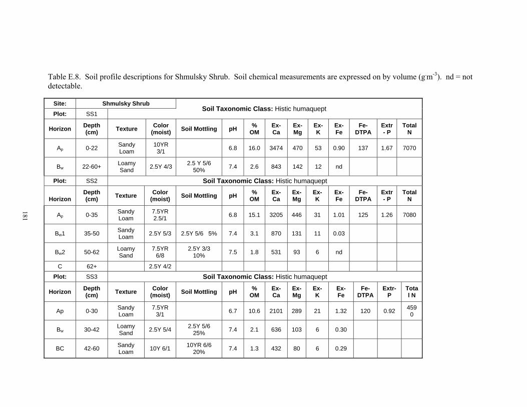
181

181

Table E.8. Soil profile descriptions for Shmulsky Shrub. Soil chemical measurements are expressed on by volume (g.m-3). nd = not detectable.

Site: Shmulsky Shrub Soil Taxonomic Class: Histic humaquept

Plot: SS1



Ex- Ca

Ex- Mg

Ex- K

Ex- Fe

Fe- DTPA

Extr- P

Total N

Ap 0-22 Sandy Loam

10YR 3/1 6.8 16.0 3474 470 53 0.90 137 1.67 7070

Bw 22-60+ Loamy Sand 2.5Y 4/3 2.5 Y 5/6

50% 7.4 2.6 843 142 12 nd

Plot: SS2 Soil Taxonomic Class: Histic humaquept



Ex- Ca

Ex- Mg

Ex- K

Ex- Fe

Fe- DTPA

Extr- P

Total N

Ap 0-35 Sandy Loam

7.5YR 2.5/1 6.8 15.1 3205 446 31 1.01 125 1.26 7080

Bw1 35-50 Sandy Loam 2.5Y 5/3 2.5Y 5/6 5% 7.4 3.1 870 131 11 0.03

Bw2 50-62 Loamy Sand

7.5YR 6/8

2.5Y 3/3 10% 7.5 1.8 531 93 6 nd

C 62+ 2.5Y 4/2

Plot: SS3 Soil Taxonomic Class: Histic humaquept



Ex- Ca

Ex- Mg

Ex- K

Ex- Fe

Fe- DTPA

Extr- P

Total N

Ap 0-30 Sandy Loam

7.5YR 3/1 6.7 10.6 2101 289 21 1.32 120 0.92 459

0

Bw 30-42 Loamy Sand 2.5Y 5/4 2.5Y 5/6

25% 7.4 2.1 636 103 6 0.30

BC 42-60 Sandy Loam 10Y 6/1 10YR 6/6

20% 7.4 1.3 432 80 6 0.29

182

182

APPENDIX F

SPECIES LIST

183

183

Table F.1. Species observed in the 24 study plots. Nomenclature is derived from the most current reports at the USDA Plants Database (USDA, 2007). A “*” in the boxes below the site codes indicates the species was found at that site. A “y” in the column titled “85” indicates it was one of the 85 species used in the vegetation ordination.

Common Name Scientific Name Species Code 85 Site Code

JN JS SBB SBC SBN SBS SO SS Red Maple Acer rubrum L. ACERUB y * * * * * * Redtop Agrostis gigantea Roth Grass4 y * * * * * * Creeping Bentgrass Agrostis stolonifera L. Grass3 y

* * * * *

Speckled Alder Alnus incana (L.) Moench ssp. rugosa (Du Roi) Clausen ALNRUG

*

Hazel Alder Alnus serrulata (Ait.) Willd. ALNSER y * * * American Hogpeanut

Amphicarpaea bracteata (L.) Fern. AMPBRA

*

Paper Birch Betula papyrifera Marsh. BETPAP * Bog Birch Betula pumila L. BETPUM * Fringed Brome Bromus ciliatus L. Grass9 * *

Bluejoint Calamagrostis canadensis (Michx.) Beauv. Grass11

* *

Tuberous Grasspink

Calopogon tuberosus (L.) B.S.P. var. tuberosus CALPUL y

* * *

Yellow Sedge Carex flava L. CARFLA y * * * * * * * Limestone Meadow Sedge Carex granularis Muhl. ex Willd. CARGRA y

* * * * *

Bottlebrush Sedge Carex hystericina Muhl. ex Willd. CARHYS y

* * * * * *

Inland Sedge Carex interior Bailey CARINT y * * * * * Hairy Sedge Carex lacustris Willd.

CARLAC y

*

184

184


JN JS SBB SBC SBN SBS SO SS Bristlystalked Sedge Carex leptalea Wahlenb. CARLEP y

* * * * * * *

Shallow Sedge Carex lurida Wahlenb. CARLUR y * * Carex sp.1 CARunk1 * Carex sp.2 CARunk2 * Dioecious Sedge Carex sterilis Willd. CARSTE y * * * * Upright Sedge Carex stricta Lam. CARSTR y * * * * Rigid Sedge Carex tetanica Schkuhr CARTET * Fox Sedge Carex vulpinoidea Michx. CARVUL y * * * * * Spotted Water Hemlock Cicuta maculata L. CICMAC

* *

Threeleaf Goldthread Coptis trifolia (L.) Salisb. COPGRO

*

Silky Dogwood Cornus amomum P. Mill. CORAMO y * * * Redosier Dogwood Cornus sericea L. CORSER y

* * * *

Shrubby Cinquefoil

Dasiphora fruticosa (L.) Rydb. ssp. floribunda (Pursh) Kartesz DASFRU y

* * * * * * *

Queen Anne's Lace Daucus carota L. DAUCAR

*

Roundleaf Sundew Drosera rotundifolia L. DROROT y

* * *

Spikerush Eleocharis R. Br. ELEOCH y * * * * * Field Horsetail Equisetum arvense L. EQUARV y * * * * * * Water Horsetail Equisetum fluviatile L. EQUFLU y * * * * * Scouringrush Horsetail Equisetum hyemale L. EQUHYE

*

Tawny Cottongrass

Eriophorum virginicum L.

ERIVIR

y * * * * * *

185

185


JN JS SBB SBC SBN SBS SO SS

Spotted Trumpetweed

Eupatoriadelphus maculatus (L.) King & H.E. Robins. EUPMAC y

* * * * * * *

Common Boneset Eupatorium perfoliatum L. EUPPER y * * * * Low Rough Aster Eurybia radula (Ait.) Nesom ASTRAD y * * * * *

Nodding Fescue Festuca subverticillata (Pers.) Alexeev Grass12

* *

Woodland Strawberry Fragaria vesca L. FRAVES y

* * * * * * *

Green Ash Fraxinus pennsylvanica Marsh. FRAPEN y * * * * * * Rough Bedstraw Galium asprellum Michx. GALASP * False Baby's Breath Galium mollugo L. GALMOL y

* * * * * *

Common Marsh Bedstraw Galium palustre L. GALPAL y

* * *

Purple Avens Geum rivale L. GEURIV y * * * American Mannagrass Glyceria grandis S. Wats Grass15 y

* *

Fowl Mannagrass Glyceria striata (Lam.) A.S. Hitchc. Grass8 y

* * * *

American Marshpennywort Hydrocotyle americana L. HYDAME y

*

Jewelweed Impatiens capensis Meerb. IMPCAP y * * Harlequin Blueflag Iris versicolor L. IRIVER y

* *

Smallhead Rush Juncus brachycephalus (Engelm.) Buch. JUNBRA y

* * * * * *

Narrowpanicle Rush

Juncus brevicaudatus (Engelm.) Fern. JUNBRE y

* * * * * *

Common Rush Juncus effusus L. JUNEFF y * * * Knotted Rush Juncus nodosus L. JUNNOD y * * * *

186

186


JN JS SBB SBC SBN SBS SO SS Juncus sp.1 JUNunk1 * * Juncus sp.2 JUNunk2 * Juncus sp.3 JUNunk3 * Common Juniper Juniperus communis L. JUNCOM * Tamarack Larix laricina (Du Roi) K. Koch LARLAR y * * * Canada Lily Lilium canadense L. LILCAN * Yellow False Pimpernell Lindernia dubia (L.) Pennell LINDUB

*

Ontario Lobelia Lobelia kalmii L. LOBKAL * * Morrow's Honeysuckle Lonicera morrowii Gray LONMOR

*

American Water Horehound

Lycopus americanus Muhl. ex W. Bart. LYCAME y

* * * * * *

Fringed Loosestrife Lysimachia ciliata L. LYSCIL y

* * *

Earth loosestrife Lysimachia terrestris (L.) B.S.P. LYSTER y * * Winged Lythrum Lythrum alatum Pursh LYTALA * Purple Loosestrife Lythrum salicaria L. LYTSAL y * *

Peppermint Mentha ×piperita L. (pro sp.) [aquatica × spicata] MENPIP

* *

Wild Mint Mentha arvensis L. MENARV y * * * * * *

Spiked Muhly Muhlenbergia glomerata (Willd.) Trin. Grass1 y

* * * * * *

Watermilfoil Myriophyllum L. MYRIO * * Sensitive Fern Onoclea sensibilis L. ONOSEN y * * * Cinnamon Fern Osmunda cinnamomea L. OSMCIN * * Royal Fern Osmunda regalis L. OSMREG * * Common Yellow Oxalis

Oxalis stricta L. OXAEUR y * * *

187

187

Common Name Scientific Name Species

Code 85 Site Code JN JS SBB SBC SBN SBS SO SS

Golden Ragwort Packera aurea (L.) A.& D. Löve PACAUR y * * * * * *

Panicgrass Panicum sp. L. Grass6 y * * * * Fen Grass of Parnassus Parnassia glauca Raf. PARGLA y

* * * * * *

Virinia Creeper Parthenocissus quinquefolia (L.) Planch. PARQUI

*

Wild Parsnip Pastinaca sativa L. PASSAT * Reed Canarygrass Phalaris arundinaea L. Grass14 * Eastern White Pine Pinus strobus L. PINSTR y

* *

Common Plantain Plantago major L. PLAMAJ * Northern Green Orchid Platanthera aquilonis Sheviak HABHYP y

* *

Fowl Bluegrass Poa palustris L. Grass13 y * Snakemouth Orchid

Pogonia ophioglossoides (L.) Ker-Gawl. POGOPH y

* * *

Arrowleaf Tearthumb Polygonum sagittatum L. POLSAG y

* * *

Quaking Aspen Populus tremuloides Michx. POPTRE * Common Cinquefoil Potentilla simplex Michx. POTSIM y

* * *

Common Selfheal Prunella vulgaris L. PRUVUL * Black Cherry Prunus serotina Ehrh. PRUSER *

Virgina Mountainmint

Pycnanthemum virginianum (L.) T. Dur. & B.D. Jackson ex B.L. Robins. & Fern. PYCVIR y

*

Tall Buttercup Ranunculus acris L. RANACR y * * * * * Bristly Buttercup Ranunculus hispidus Michx.

RANHIS y * * *

188

188

Common Name Scientific Name Species Code 85

Site Code JN JS SBB SBC SBN SBS SO SS

Alderleaf Buckthorn Rhamnus alnifolia L'Hér. RHAALN y

* * *

Multiflora Rose Rosa multiflora Thunb. ex Murr. ROSMUL y * * *

American Red Raspberry Rubus idaeus L. RUBIDA y

* *

Dwarf Red Blackberry Rubus pubescens Raf. RUBPUB y

* * * *

Sageleaf Willow Salix candida Flueggé ex Willd. SALCAN y * * * Silky Willow Salix sericea Marsh. SALSERIC y * * * * * Autumn Willow Salix serissima (Bailey) Fern. SALSERIS y * * * * Green Bulrush Scirpus atrovirens Willd. SCIATR y * * * * Rufous Bulrush Scirpus pendulus Muhl. SCIPEN * * Marsh Skullcap Scutellaria galericulata L. SCUEPI * * Strict Blue-eyed Grass Sisyrinchium montanum Greene SISMON

* *

Hemlock Waterparsnip Sium suave Walt. SIUSUA

*

Giant Goldenrod Solidago gigantea Ait. SOLGIG y * * * * * * * * Roundleaf Goldenrod Solidago patula Muhl. ex Willd. SOLPAT y

* * * * * * *

Bog Goldenrod Solidago uliginosa Nutt. SOLULI y * * * * * Sphagnum Moss Sphagnum L. SPHAG * White Meadowsweet

Spiraea alba Du Roi var. latifolia (Ait.) Dippel SPILAT y

* * * * *

Nodding Lady's Tresses Spiranthes cernua (L.) L.C. Rich. SPICER y

* * * * *

Purplestem Aster Symphyotrichum puniceum (L.) A.& D. Löve var. puniceum SYMPUN y

* * * * * *

Skunk Cabbage Symplocarpus foetidus (L.) Salisb. ex Nutt.

SYMFOE

y

* * * * * * * *

189

189


JN JS SBB SBC SBN SBS SO SS King of the Meadow Thalictrum pubescens Pursh. THAPOL y

* * *

Eastern Marsh Fern

Thelypteris palustris Schott THEPAL y

* * * * * * * *

Eastern Poison Ivy

Toxicodendron radicans (L.) Kuntze TOXRAD

* *

Poison Sumac Toxicodendron vernix (L.) Kuntze TOXVER y

* *

Virginia Marsh St. Johnswort Triadenum virginicum (L.) Raf. HYPVIR y

* * * *

Starflower Trientalis borealis Raf. TRIBOR * Broadleaf Cattail Typha latifolia L. TYPLAT y * * * * * American Elm Ulmus americana L. ULMAME * Unknown 1 UNK1 * Unknown 2 UNK2 * Unknown Graminoid10 Grass10 * * Unknown Graminoid2 Grass2 y * * * * Unknown Graminoid5 Grass5 * Unknown Graminoid7 Grass7 y * * Highbush Blueberry Vaccinium corymbosum L. VACCOR y

* * *

Southern Arrowwood Viburnum dentatum L. VIBDEN y

* *

Violet Viola Sp. L. VIOLA * Species Richness 79 39 50 43 52 36 67 57

190

190

LITERATURE CITED

Aldrige, L. P. and G. J. Churchman. 1991. The role of iron in the weathering of a climosequence of soils derived from schist. Australian journal of soil research 29:387-398. Auclair, A. D. 1979. Factors affecting tissue nutrient concentrations in a Scirpus-Equisetum wetland. Ecology 60:337-348. Atkinson, C. J. 1991. The flux and distribution of xylem sap calcium to adaxial and abaxial epidermal tissue in relation to stomatal behaviour. Journal of Experimental Botany 42:987-993. Beals, E. W. 1984. Bray-Curtis ordination: an effective strategy for analysis of multivariate ecological data. Advances in Ecological Research 4:1-55. Bedford, B. L., M. R. Walbridge, and A. Aldous. 1999. Patterns in nutrient availability and plant diversity of temperate North American wetlands. Ecology 80:2151-2169. Bedford, B. L. and K. S. Godwin. 2003. Fens of the United States: Distribution, characteristics, and scientific connection versus legal isolation. Wetlands 23:608-629. Blake, G. R. and K. H. Hartge. 1986. Bulk Density. Pages 363-382 in A. Klute, editor. Methods of Soil Analysis Part 1. Soil Science Society of America, Inc., Madison, Wisconsin, USA. Bonnier, G. 1894. Remarques sur les différences que presénte l’Ononis Natrix cultivé sur un sol calcaire on sur un sol sans calcaire (Comments on the differences presented by natrix cultivars in l'Ononis on a calcareous soil or on a soil without limestone). Bulletin of the Botanical Society of France xli. Bowden, W. B. 1987. The biogeochemistry of nitrogen in freshwater wetlands. Biogeochemistry 4:313-348. Bowles, M. L., P. D. Kelsey, and J. L. McBride. 2005. Relationships among environmental factors, vegetation zones, and species richness in a North American calcareous prairie fen. Wetlands 25:685-696. Boyd, C. E. 1966. The elemental composition of several freshwater algae. Ph.D. Dissertation, Auburn University, Auburn, Alabama, USA. Boyd, C. E. and L. W. Hess. 1970. Factors influencing shoot production and mineral nutrient levels in Typha latifolia. Ecology 51:296-300. Boyer, M. H. L. and B. D. Wheeler. 1989. Vegetation patterns in spring-fed calcareous fens: calcite precipitation and constraints on fertility. Journal of Ecology 77:597-609.

191

Brady, N. C. and R. R. Weil. 2000. The nature and properties of soils. Prentice-Hall Inc. Upper Saddle River, New Jersey, USA. Bremmer, J. M. and C. S. Mulvaney. 1986. Nitrogen-Total. Pages 595-624 in A. Klute, editor. Methods of Soil Analysis Part 2. Soil Science Society of America, Inc., Madison, Wisconsin, USA. Bremmer, J. M. and K. Shaw. 1958. Denitrification in soil. I. Methods of investigation. Journal of Agricultural Science 51:22-39. Broadley, M. R., H.C. Bowen, H.C. Cotterlii, J. P. Hammond, M. C. Meacham, A. Mead, and P. J. White. 2003. Variation in the shoot calcium content of angiosperms. Journal of Experimental Botany 54:1431-1446. Brooks, K. N., P. F. Ffolliott, H. M. Gregersen, and L. F. DeBano. 1997. Hydrology and the management of watersheds, 2nd Edition. Iowa State University Press, Ames, Iowa, USA. Clarkson, D. T. 1965. Calcium uptake by calcicole and calcifuge species in the genus Agrostis L. Journal of Ecology 53:427-435. Clesceri, L. S., A. E. Greenberg, R. R. Trussell (editors). 1989. Standard methods for the examination of water and wastewater, 20th edition. American Public Health Association, American Water Works and the Water Pollution Control Federation, Washington, D.C., USA. Cobbaert, D., L. Rochefort, and J. S. Price. 2004. Experimental restoration of a fen plant community after peat mining. Applied Vegetation Science 7:209-220. Contejean, C. 1881. Géographie botanique, influence du terrain sur la vegetation. (Geographic botany, The influence of the ground on vegetation). 8vo. Paris, France. Da Silva, D. L. R., L. P. Ruiz, C. J Atkinson, and T. A. Mansfield. 1994. Physiological disturbance caused by high rhizosphere calcium in the calcifuge, Lupinus luteus. Journal of Experimental Botany 45:585-590. Dean, W. E. 1974. Determination of carbonate and organic matter in calcareous sediments and sedimentary rocks by loss on ignition: comparison with other methods. Journal of Sedimentary Petrology 44:242-248. Douglas, M. E. & J. A. Endler. 1982. Quantitative matrix comparisons in ecological and evolutionary investigations. Journal of Theoretical Biology 99:777-795. Drexler, J. Z., and B. L. Bedford. 2002. Pathways of nutrient loading and impacts on plant diversity in a New York peatland. Wetlands 22:263-281.

192

Dyck, A. W. J and R. R. McKibbin. 1935. The non-protein nature of a fraction of soil organic nigtrogen. Canadian Journal of Research 13B:264-298. Eggers, S. D. and D. M. Reed, 1987. Wetland plants and plant communities of Minnesota and Wisconsin. US Army Corps of Engineers, St. Paul, Minnesota., USA. Ehrenberg, P. 1919. Das Kalk-Kali-Gesetz. Parey, Berlin, Germany. Ehrenfeld, J.G. and J. P. Schneider. 1993. Responses of forested wetland vegetation to perturbations of water chemistry and hydrology. Wetlands 13:122-129. Elkington T. T., and S. Woodell. 1963. Potentilla-fruticosa L. (Dasiphora fruticosa (L). Rydb.). Journal of Ecology 51: 769-781. Gauch, H.G. 1972. Inorganic Plant Nutrition. Dowden, Hutchinson & Ross, Stroudsburg, Pennsylvania, USA. Gee, G. W. and J. W. Bauder. 1986. Particle-size Analysis. Pages 383-411 in A. Klute, editor. Methods of Soil Analysis Part 1. Soil Science Society of America, Inc., Madison, Wisconsin, USA. Gleason, H. A. and A. Cronquist. 1991. Manual of vascular plants of northeastern United States and adjacent Canada, second edition. New York Botanical Garden, Bronx, New York, USA. Godwin, K.S., J.P. Shallenberger, D. J. Leopold, B. L. Bedford. 2002. Linking landscape properties to local hydrogeologic gradients and plant species occurrence in minerotrophic fens of New York State, USA: A hydrogeologic setting (HGS) framework. Wetlands 22:722-737. Grootjans, A. P., R. van Diggelen, M. J. Wassen, and W.A. Wiersinga. 1988. The effects of drainage on groundwater quality and plant species distribution in stream valley meadows. Vegetatio 75:37-48. Hach Company, 1992. DR/2000 Spectrophotometer Procedures Manual. Hach Company World Headquarters, Loveland, Colorado, USA. Hamze M, M. Nimah, and M. Zaabout. 1984. Effectiveness of six digestion procedures to evaluate the status of major elements (Ca, K, Mg, and Na) in citrus leaves. Communications in Soil Science and Plant Analysis 15:1135-1145. Higley, W. K. 1880. On the microscopic crystals contained in plants. The American Naturalist 14:720-725.

193

Hope-Simpson, J. 1938. The chalk flora of the Lower Greensand: its uses in interpreting the calciole habit. Journal of Ecology 26:218-235. Iljin, W. S. 1936. Zur Physiologie der kalkfeindlichen Pflanzen. Beihefte zum Botanischen Centralblatt 54:569-598. Jones, J. B., Jr. 2001. Laboratory guide for conducting soil tests and plant analysis. CRC Press, New York, New York, USA. Kearsley, J. B. 1999. The natural communities of Massachusetts: Palustrine section. Unpublished draft. Massachusetts Natural Heritage and Endangered Species Program, Westborough, Massachusetts, USA. Kerner von Marilaun, A. 1895. The Natural History of Plants. Blackie and Son, London, England. Kinzel, H. 1963. Zellsaftanalysen zum pflanzlichen Calcium- und Säurestoffwechsel und zum Problem der Kalk- und Silikatpflanzen. Protoplasma 57:522-555. Kinzel, H. 1983. Physiological Plant Ecology III: Responses of the chemical and biological environment. Chapter 6: Influence of Limestone, Silicates and Soil pH on Vegetation. Springer-Verlag, New York, New York, USA. Komor, S. C. 1994. Geochemistry and hydrology of a calcareous fen with the Savage Fen wetlands complex, Minnesota, USA. Geochimica et Cosmochimica Acta 58:3353-3367. Le Gales, Y., A. Lamart, and R. Heller. 1980. Fixation due calcium par des fractions macromoleculaires solubles iolees a partir de vegetaux superieurs (Calcium fixing protiens in plants). Physiologie Vegetale 18:431-441. Lee, J. A. 1999. The calcicole-calcifuge problem revisited. Advances in Botanical Research. 29:1-29 Loneragan, J. F., K. Snowball, W. J. Simmons. 1968. Response of plants to calcium concentration in solution culture. Australian Journal of Agricultural Research 19:845-857. Lucassen, E. C. H. E. T., A. J. P. Smolders, G. Boedeltje, P. J. J. van den Munckhof, J. G. M. Roelofs. 2006. Groundwater input affecting plant distribution by controlling ammonium and iron availability. Journal of Vegetation Science 17:425-43. Lynch, J. and A. Lauchli. 1985. Salt stress disturbs the calcium nutrition of barley (Hordeum vulgare L.). New Phytologist 99:345-354.

194

Marosz, A. 2004. Effect of soil salinity on nutrient uptake, growth, and decorative value of four ground cover shrubs. Journal of Plant Nutrition 27:977-989. Marschner, H. 1995. Mineral Nutrition of Higher Plants, 2nd Edition. Academic Press: New York, New York, USA. McLean, E. O. 1986. Soil pH and Lime Requriement. Pages 199-224 in A. Klute, editor. Methods of Soil Analysis Part 2. Soil Science Society of America, Inc., Madison, Wisconsin, USA. McCune, B. and J. B. Grace. 2002. Analysis of Ecological Communities. MjM Software Design, Gleneden Beach, Oregon, U.S.A. McCune, B. and M. J. Mefford. 1999. PC-ORD. Multivariate Analysis of Ecological Data. Version 5.0. MjM Software Design, Gleneden Beach, Oregon, U.S.A. Miller, E. L., A. P. Bimbo, S. M. Barlow and B. Sheridan. 2007. Repeatability and reproducibility of determination of the nitrogen content of fishmeal by the combustion (Dumas) method and comparison with the Kjeldahl method: Interlaboratory study. Journal of AOAC International 90:6-20. Mills, H. A. and J. B. Jones, Jr. 1991. Plant Analysis Handbook II. Micromacro Publishing, Athens, Georgia, USA. Mitsch, W. J. and J. G. Gosselink. 1993. Wetlands, 2nd Edition. John Wiley and Sons, Inc. New York, New York, USA. MNHESP (Massachusetts Natural Heritage and Endangered Species Program), 2004. List of Endangered, Threatened, & Special Concern Species, in Code of Massachusetts Regulations, 321 CMR 10.90. Massachusetts Division of Fisheries & Wildlife, Westborough, Massachusetts, USA. Molisch, H. 1918. Über den mikrochemischen Nachweis und die Verbreitung gelöster Oxalate im Pflanzenreiche. Flora 11:60-70. Motzkin, G. 1994. Calcareous fens of western New England and adjacent New York State. Rhodora 96:44-68. Nägeli, C. W. von, 1865. Ueber die Bedingungen des Vorkommens von Arten und Varietaten innerhalb ihres Verbreitungsbezirkes (About the conditions of the occurence of kinds and varieties within a spreading district). Sitzungsber. d. Konigl. Bayrischen Akademie. National Atlas. 2006. National Atlas of the United States. http://www.nationalatlas.gov/index.html. Last modified: May 22, 2006

195

Nekola, J. C. 2004. Vascular plant compositional gradients within and between Iowa fens. Journal of Vegetation Science 15:771-780. NOAA, National Oceanic and Atmospheric Administration. 2006. Local climatological data: Annual summary with comparative data for Albany, New York. NCDC Asheville, North Carolina. NRCS, Natural Resources Conservation Service. 2003. Climate Analysis for Wetlands by State: http://www.wcc.nrcs.usda.gov/climate/wetstate.html. Accessed 10/2006. Olbe, M. and M. Sommarin. 1991. ATP-dependent calcium transport in wheat root plasma membrane vesicles. Physiologia Plantarum 83:535-543. Palta, J. P. and E. J. Stadelmann. 1980. On simultaneous transport of water and solute through plant cell membranes: Evidence for the absence of solvent drag effect and insensitivity of the reflection coefficient. Physiologia Plantarum 50:83-91. Picking, D.J. 2002. Vegetation patterns and associated hydrogeochemical cycles in a calcareous sloping fen of southwestern Massachusetts. Ph.D. Dissertation. University of Massachusetts, Amherst, Massachusetts, USA. Picking, D. J. and P. L. M. Veneman. 2004. Vegetation patterns in a calcareous sloping fen of southwestern Massachusetts, USA. Wetlands 24:514-528. Portis, A. R., C. Ja Chon, A. Mosbach, and H. W. Heldt. 1977. Fructose- and Sedoheptulosebis-phosphatase. The sites of possible control of CO2 fixation by light dependent changes of the stromal Mg2+ concentration. Biochimica et Biophysica Acta 461:313-325. Reader, R. J. 1990. Competition constrained by low nutrient supply: an example involving Hieracium floribundum Wimm and Grab. Compositaceae. Functional Ecology 4:573-577. Reschke, C. 1990. Ecological Communities of New York State. New York Natural Heritage Program, N.Y.S. Department of Environmental Conservation, Latham, New York, USA. Richardson, C. J., and P. E. Marshall. 1986. Processes controlling movement, storage, and export of phosphorus in a fen peatland. Ecological Monographs 56:279–302. Robichaud, B. and K. H. Anderson. 1994. Plant communities of New Jersey – A study in landscape diversity. Rutgers University Press, New Brunswick, New Jersey, USA. Römheld, V. 1987. Different strategies for iron acquisition in higher plants. Physiologia Plantarum 70:231-234.

196

Rorison, I. H. 1960. Some experimental aspects of the calcicole-calcifuge problem. I. The effects of competition and mineral nutrition upon seedling growth in the field. Journal of Ecology 48:585-599. Ruiz, L.P., C. J. Atkinson, T. A. Mansfield. 1993. Calcium in the xylem and its influence on the behavior of stomata. Philosophical Transactions of the Royal Society of London B 341:67-74. Salisbury, E. J. 1920. The significance of the calcicolous habit. Journal of Ecology 8:202. Saltonstall K., 2002. Cryptic invasion by a non-native genotype of the common reed, Phragmites australis, into North America. Proceedings of the National Academy of Sciences of the United States of America 99:2445-2449 SAS Institute. 2004. SAS Version 9.1.3. SAS Institute, Cary, North Carolina, USA. Scanu, R. J., 1988. Soil Survey of Berkshire County Massachusetts. United States Department of Agriculture, Soil Conservation Service. In cooperation with Massachusetts Agricultural Experiment Station. Schot. P. P. and M. J. Wassen, 1993. Calcium concentration in wetland groundwater in relation to water sources and soil conditions in the recharge area. Journal of Hydrology 141:197-217. Sendtner. O. 1860. Die Vegetationsverhaltnisse des Baverischen Waldes. Munchen. Germany. Shaw, S. C. 2003. Do pollen assemblages in surface samples reflect community composition? A study of a Massachusetts fen. M.S. Thesis. University of Massachusetts, Amherst, Massachsetts, USA. Shrimper, A. F. W. 1898. Plant Geography upon a Physiological Basis. Engl. Ed., Oxford, 1903. Sjörs, H. 1950. On the relation between vegetation and electrolytes in North Swedish mire water. Oikos 2:242-258. Slack, N. G., D. H. Vitt, and D. G. Horton. 1980. Vegetation gradients of minerotrophically rich fens in western Alberta. Canadian Journal of Botany 58:330-350. Solomon, E. P., L. R. Berg, D. W. Martin, and C. Villee. 1996. Biology 4th Edition. Saunders college publishing, New York, New York, USA. Soil Survey Staff, 1993. Soil Survey Manual. USDA Handbook No. 18. United States Government Printing Office, Washington, D. C., USA.

197

Soltanpour, P. N. and A. P. Schwab. 1977. A new soil test for simultaneous extraction of macro- and micronutrients in alkaline soils. Communications in soil science and plant analysis. 8:195-207. Stewart, B. A., L. K. Porter, and F. E. Clark. 1963. The reliability of a micro-Dumas procedure for determining total nitrogen in soil. Soil Science Society of America Proceedings. 28:366-368. Tansley A. G. 1917. On competition between Galium Saxatile L. (G. Hercynicum Weig.) and Galium Sylvestre Poll. (G. Asperum Schreb.) on different types of soil. The Journal of Ecology 5:173-179. Taylor, K. 1997. Geum rivale L. Journal of Ecology 85:721-731. Thomas, G. W. 1986. Exchangeable Cations. Pages 159-165 in A. Klute, editor. Methods of Soil Analysis Part 2. Soil Science Society of America, Inc., Madison, Wisconsin, USA. Thompson, R., J. A. Parkinson, S. R. Band, R. E. Spencer. 1997. A comparative study of leaf nutrient concentrations in a regional herbaceous flora. New Phytologist 136:679-689. Tyler, G. and L. Ström. 1995. Differing organic acid exudation patterns explain calcifuge and acidifuge behaviour of plants. Annals of Botany 75:75-78. USDA, NRCS. 2007. The PLANTS Database (http://plants.usda.gov, 3 October 2007). National Plant Data Center, Baton Rouge, Louisianna, USA. Vitt, D. H., P. Achuff, and R. E. Andrus. 1975. The vegetation and chemical properties of patterned fens in the Swan Hills, north central Alberta. Canadian Journal of Botany 53: 2776-2795. Vitt, D. H. and W. Chee. 1990. The relationship of vegetation to surface water chemistry and peat chemistry in fens of Alberta, Canada. Vegetatio 89:87-106. Waldren, S., J. R. Etherington, and M. S. Davies. 1987. Comparative Studies of Plant Growth and Distribution in Relation to Waterlogging. XIV. Iron, Manganese, Calcium and Phosphorus Concentrations in Leaves and Roots of Geum rivale L. and G. urbanum L. Grown in Waterlogged Soil. New Phytologist 106:689-696. Walker, C. J. and J. D. Weinstien, 1991. Further characterization of the magnesium chelatase in isolated developing cucumber chloroplasts - substrate-specificity, regulation, intactness, and ATP requirements. Plant Physiology 95:1189-1196

198

Watson, M. E. and T. L. Galliher. 2001. Comparison of Dumas and Kjeldahl methods with automatic analyzers on agricultural samples under routine rapid analysis conditions. Communications in Soil Science and Plant Analysis 32:2007-2019. Weatherbee, P.B. 1996. Flora of Berkshire County Massachusetts. The Studley Press, Inc., Dalton, Massachusetts, USA. Weatherbee, P.B. and G. E. Crow. 1992. Natural plant communities of Berkshire county, Massachusetts. Rhodora 94:171-209. White, P. J. 1998. Calcium channels in the plasma membrane of root cells. Annals of Botany 81:173-183. White, P. J. 2001. The pathways of calcium movement to the xylem. Journal of Experimental Botany 52:891-899. White, P. J. and M. R. Broadley, 2003. Calcium in plants. Annals of Botany 92:487-511. Woolhouse, H. W. 1966. The effect of bicarbonate on the uptake of iron in four related grasses. New Phytologist 65:372-375. Zampella, R. A. and K. J. Laidig. 1997. Effect of watershed disturbance on Pinelands stream vegetation. Journal of the Torrey Botanical Society 124:52-66. Zen, E. and J. H. Hartshorn. 1966. Geologic map of the bashbish quadrangle, Massachusetts, Connecticut, and New York. Department of the Interior, United States Geological Survey. Washington, D.C., USA. Zen, E. and N. M. Ratcliffe. 1971. Bedrock geologic map of the Egremont quadrangle and adjacent areas, Berkshire County, Massachusetts, and Colombia County, New York. Department of the Interior, United States Geological Survey. Washington, D.C., USA.

a comparison of environmental substrate gradients and

Documents