a benchmark study of optimization search algorithms rev. 01.10 a benchmark study of optimization...

BMK-3022 Rev. 01.10

A Benchmark Study of Optimization Search Algorithms

Page | 1

N. Chase, M. Rademacher, E. Goodman Michigan State University, East Lansing, MI

R. Averill, R. Sidhu Red Cedar Technology, East Lansing, MI

Abstract. A thorough study was conducted that benchmarks the efficiency and robustness of several optimization algorithms. In particular, the hybrid adaptive method, SHERPA, in HEEDS Professional, was compared to several existing methods. These algorithms were tested on a broad set of benchmark problems, each of which emphasizes a different set of features commonly found in engineering optimization problems. It was concluded that the SHERPA algorithm is significantly more efficient and robust for these problems than the other methods in the study.

1. Introduction

Engineers in all major industries are rapidly adopting automated design optimization technology. The potential for delivering better designs in less time, compared to manual optimization approaches, makes automated design optimization very attractive from both a technical and a business standpoint. However, two primary barriers prevent engineers from realizing the true value of optimization across broad classes of problems.

First, choosing the appropriate optimization search algorithm for a given problem depends upon the type of design space that has been defined. But the characteristics of the design space are typically not known until it has been explored, which is the primary role of the search algorithm. Faced with this “chicken and egg” problem, selecting the best method to use and then tuning its parameters is a time-consuming process, largely based on trial and error. Often engineers must solve the same optimization problem multiple times in order to identify the method or settings that yield the optimal solution. This may increase the overall time to solution by several factors, which is unacceptable under any circumstances but especially when design evaluations are computationally expensive.

Consequently, the availability of an algorithm that performs well over a wide range of problems can eliminate manual tuning and yield the desired

solution within a single run, reducing manual effort and design cycle time significantly.

Second, some algorithms are not efficient enough to be used for large-scale optimization studies or those involving expensive design evaluations. If a single evaluation requires several hours to complete, and a few hundred evaluations are needed to identify an optimized solution, then weeks or even months of CPU time may be required. In this case, reducing the total number of evaluations needed to find an optimized design has a large impact on the solution time, and the difference in performance between two algorithms can translate into days or even weeks of CPU time.

The objective of this study was to compare several of the available algorithms to assess their performance relative to these two issues: effectiveness and efficiency over a wide range of problems.

1.1 Design Optimization Problem Statement

Mathematically speaking, the optimization problem of interest here may be stated as:

Minimize (or maximize):

f(x1,x2, …,xn)

such that:

gi(x1,x2,…,xn) ≤ 0, i=1,2,…,p


Page | 2

hj(x1,x2,…,xn) = 0, j=1,2,…,q

where:

f(x1,x2,…,xn) is the objective function

gi(x1,x2,…,xn) are the p inequality constraints,

hj(x1,x2,…,xn) are the q equality constraints, and

(x1,x2,…,xn) are the n design variables

The functions f, gi, and hj are responses of the system, while the design variables (x1,x2,…,xn) are the inputs. A particular design candidate k is obtained by assigning values to all of the design variables (x1,x2,…,xn)k. In general, the responses f, gi, and hj are not known analytical functions. Rather, the values of these functions can be calculated at a finite number of points, or designs, based on the strategy embedded in the optimization algorithm. The evaluation of these responses for a given design may be performed using an analysis model such as a finite element model, a CFD model, a multi-body dynamics model, or any other predictive model. The role of an optimization algorithm is to solve the above problem using as few design evaluations as possible.

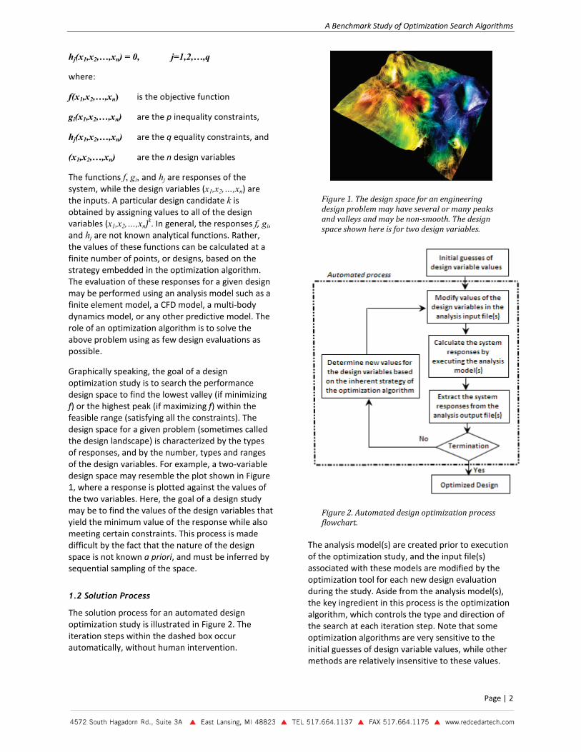
Graphically speaking, the goal of a design optimization study is to search the performance design space to find the lowest valley (if minimizing f) or the highest peak (if maximizing f) within the feasible range (satisfying all the constraints). The design space for a given problem (sometimes called the design landscape) is characterized by the types of responses, and by the number, types and ranges of the design variables. For example, a two-variable design space may resemble the plot shown in Figure 1, where a response is plotted against the values of the two variables. Here, the goal of a design study may be to find the values of the design variables that yield the minimum value of the response while also meeting certain constraints. This process is made difficult by the fact that the nature of the design space is not known a priori, and must be inferred by sequential sampling of the space.

1.2 Solution Process

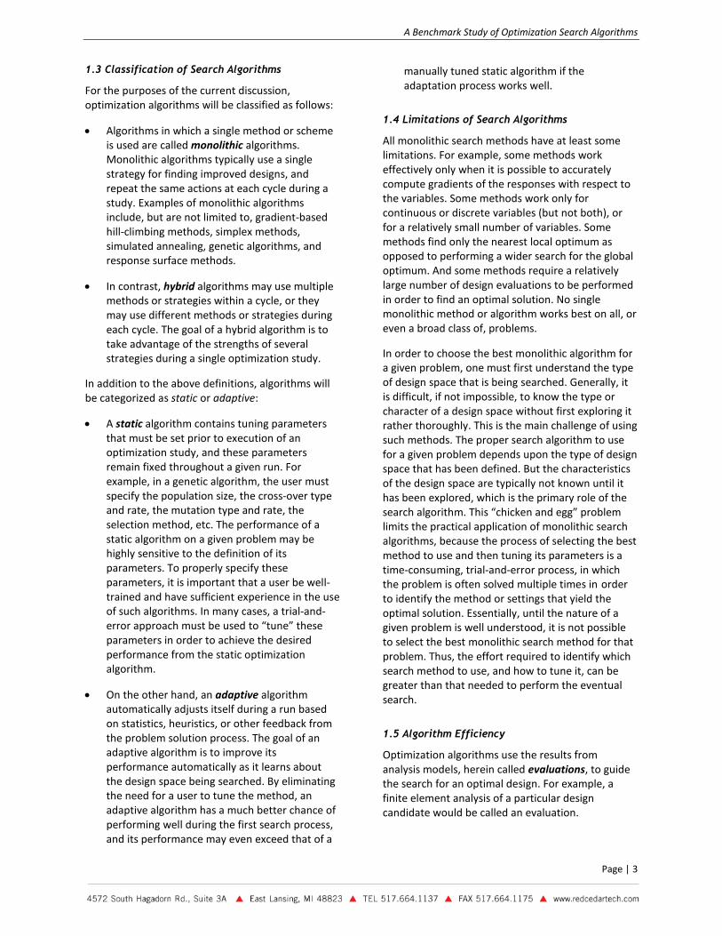
The solution process for an automated design optimization study is illustrated in Figure 2. The iteration steps within the dashed box occur automatically, without human intervention.

Figure 1. The design space for an engineering design problem may have several or many peaks and valleys and may be non-smooth. The design space shown here is for two design variables.

Figure 2. Automated design optimization process flowchart.

The analysis model(s) are created prior to execution of the optimization study, and the input file(s) associated with these models are modified by the optimization tool for each new design evaluation during the study. Aside from the analysis model(s), the key ingredient in this process is the optimization algorithm, which controls the type and direction of the search at each iteration step. Note that some optimization algorithms are very sensitive to the initial guesses of design variable values, while other methods are relatively insensitive to these values.


Page | 3

1.3 Classification of Search Algorithms

For the purposes of the current discussion, optimization algorithms will be classified as follows:

• Algorithms in which a single method or scheme is used are called monolithic algorithms. Monolithic algorithms typically use a single strategy for finding improved designs, and repeat the same actions at each cycle during a study. Examples of monolithic algorithms include, but are not limited to, gradient-based hill-climbing methods, simplex methods, simulated annealing, genetic algorithms, and response surface methods.

• In contrast, hybrid algorithms may use multiple methods or strategies within a cycle, or they may use different methods or strategies during each cycle. The goal of a hybrid algorithm is to take advantage of the strengths of several strategies during a single optimization study.

In addition to the above definitions, algorithms will be categorized as static or adaptive:

• A static algorithm contains tuning parameters that must be set prior to execution of an optimization study, and these parameters remain fixed throughout a given run. For example, in a genetic algorithm, the user must specify the population size, the cross-over type and rate, the mutation type and rate, the selection method, etc. The performance of a static algorithm on a given problem may be highly sensitive to the definition of its parameters. To properly specify these parameters, it is important that a user be well-trained and have sufficient experience in the use of such algorithms. In many cases, a trial-and-error approach must be used to “tune” these parameters in order to achieve the desired performance from the static optimization algorithm.

• On the other hand, an adaptive algorithm automatically adjusts itself during a run based on statistics, heuristics, or other feedback from the problem solution process. The goal of an adaptive algorithm is to improve its performance automatically as it learns about the design space being searched. By eliminating the need for a user to tune the method, an adaptive algorithm has a much better chance of performing well during the first search process, and its performance may even exceed that of a

manually tuned static algorithm if the adaptation process works well.

1.4 Limitations of Search Algorithms

All monolithic search methods have at least some limitations. For example, some methods work effectively only when it is possible to accurately compute gradients of the responses with respect to the variables. Some methods work only for continuous or discrete variables (but not both), or for a relatively small number of variables. Some methods find only the nearest local optimum as opposed to performing a wider search for the global optimum. And some methods require a relatively large number of design evaluations to be performed in order to find an optimal solution. No single monolithic method or algorithm works best on all, or even a broad class of, problems.

In order to choose the best monolithic algorithm for a given problem, one must first understand the type of design space that is being searched. Generally, it is difficult, if not impossible, to know the type or character of a design space without first exploring it rather thoroughly. This is the main challenge of using such methods. The proper search algorithm to use for a given problem depends upon the type of design space that has been defined. But the characteristics of the design space are typically not known until it has been explored, which is the primary role of the search algorithm. This “chicken and egg” problem limits the practical application of monolithic search algorithms, because the process of selecting the best method to use and then tuning its parameters is a time-consuming, trial-and-error process, in which the problem is often solved multiple times in order to identify the method or settings that yield the optimal solution. Essentially, until the nature of a given problem is well understood, it is not possible to select the best monolithic search method for that problem. Thus, the effort required to identify which search method to use, and how to tune it, can be greater than that needed to perform the eventual search.

1.5 Algorithm Efficiency

Optimization algorithms use the results from analysis models, herein called evaluations, to guide the search for an optimal design. For example, a finite element analysis of a particular design candidate would be called an evaluation.


Page | 4

Using fewer evaluations to find an optimized design is very important because often each evaluation can require a significant amount of CPU time. For example, a nonlinear finite element simulation may require from several hours to several days of CPU time. If a few hundred evaluations are needed to identify an optimized solution, then weeks or even months of CPU time may be required. For this reason, reducing the total number of evaluations has a large impact on the time required to find an optimized design. The difference between two algorithms can be days or even weeks of CPU time, which has a significant impact on the ability to meet deadlines.

When using automated optimization techniques, there are only three ways to reduce the overall time required to complete an optimization study:

1. Perform fewer evaluations 2. Perform shorter evaluations 3. Perform multiple evaluations

simultaneously, in parallel

Because the latter two approaches are generally independent of the search method, the focus of the current study is to identify those methods that require fewer evaluations to find an optimal solution across a wide range of problems. Therefore, herein an algorithm’s efficiency is measured in terms of the total number of evaluations required to find the optimal design or a design of a specified performance level.

1.6 Algorithm Robustness

If multiple optimization runs are performed using the same method on a given problem, the search path taken by an optimization algorithm will generally be different in each run, depending on its starting conditions. This means that the number of evaluations required to achieve a given level of design performance can be quite different from run to run. More importantly, the final results of several runs using the same algorithm may not be the same – that is, each run may fall short in some way from finding the optimal solution. These differences depend upon the starting conditions of the search, including the baseline design or initial set of designs. When comparing the performance of optimization methods in a benchmark study such as this one, multiple runs of each algorithm on each problem must be performed to more accurately assess the mean and variation of the method’s performance.

Further, the effectiveness of a search method may be very different from problem to problem. Since most algorithms are intended for a specific type of problem, wide variations in performance are commonly found for the same algorithm across several different problems.

Ideally, the performance of an optimization algorithm should be similar under all sorts of different starting conditions and on all sorts of different problems. Such an algorithm is said to be robust. This property is important for instilling confidence in the results of an algorithm, as well as for reducing the number of trial runs and the average number of evaluations in each run.

1.7 Objectives of the Current Study

In this study, the efficiency and robustness of several optimization algorithms were investigated on a set of benchmark problems. The algorithms under consideration were: SHERPA [1], Adaptive Simulated Annealing (ASA) [2], Genetic Algorithm (GA) [3], Sequential Quadratic Programming (NLPQL) [4] and a response surface method [5]. These widely used methods are available within commercial optimization software packages, as described below.

2. Overview of the Optimization Algorithms

A brief description of the methods considered in this study is presented in this section. A detailed mathematical formulation of the methods is left to the references cited.

2.1 SHERPA

SHERPA is a proprietary hybrid and adaptive search strategy available within the HEEDS Professional software code [1]. During a single parametric optimization study, SHERPA uses the elements of multiple search methods simultaneously in a unique blended manner. This approach attempts to take advantage of the best attributes of each method. Attributes from a combination of global and local search methods are used, and each participating approach contains internal tuning parameters that are modified automatically during the search according to knowledge gained about the nature of the design space.

This evolving knowledge about the design space also determines when and to what extent each approach contributes to the search. In other words, SHERPA efficiently learns about the design space and adapts


Page | 5

itself so as to effectively search many kinds of design spaces, even very complicated ones. SHERPA is a direct optimization algorithm in which all function evaluations are performed using the actual model, as opposed to using an approximate response surface model. SHERPA does not require solution gradients to exist. The only parameter that must be specified by the user is the number of allowable evaluations.

2.2 Adaptive Simulated Annealing (ASA)

Adaptive Simulated Annealing (ASA) [2] is capable of finding global optima, and it is not dependent on solution gradients. In this paper, numerical studies use an implementation of the ASA algorithm that contains 20 tunable parameters. In the current study, the following default parameter values were used:

• Num of Designs Conv Check: 5 • Convergence Epsilon: 1.0E-8 • Rel Rate of Param Annealing: 1.0 • Rel Rate of Cost Annealing: 1.0 • Rel Rate of Param Quenching: 1.0 • Rel Rate of Cost Quenching: 1.0 • Max Num of Failed Designs: 5 • Init Param Temperature: 1.0 • Reanneal Parameters: Yes • Reanneal Cost Function: Yes • Num of Des Before Reanneal: 1000 • Num of Accept Des Before Reanneal: 100 • Min Ratio of Accept Des Before Reanneal: 1.0E-6 • Rel Grad Step for Reanneal: 0.001 • Penalty Base: 0.0 • Penalty Multiplier: 1000 • Penalty Exponent: 2 • Failed Run Penalty Value: 1.0E30 • Failed Run Objective Value: 1.0E30

In addition, the parameter Max Num of Generated Designs was altered to perform the desired number of evaluations. Therefore, 19 of the 20 tunable parameters for ASA were left at their default values.

2.3 Genetic Algorithm (GA)

GA is a multi-point, evolutionary search method that performs global exploration of the design space while searching for an optimal solution [3]. It does not require the calculation of solution gradients. In this paper, numerical studies use an implementation of the multi-island GA that contains 16 tunable parameters. In the current study, the following default parameter values were used:

• Rate of Crossover: 1.0 • Rate of Mutation: 0.01 • Rate of Migration: 0.01 • Interval of Migration: 5 • Elite Size: 1 • Rel Tournament Size: 0.5 • Penalty Base: 0.0 • Penalty Multiplier: 1000 • Penalty Exponent: 2 • Max Failed Runs: 5 • Failed Run Penalty Value: 1.0E30 • Failed Run Objective Value: 1.0E30 • Default Variable Bound: 1000

The parameters Sub-Population Size and Number of Generations were altered for each run to improve the search while assuring that the desired number of evaluations was performed. The Number of Generations was maintained above 9 for the lower evaluation runs and generally was set much higher for the larger evaluation runs. Therefore, 13 of the 16 tunable parameters for GA were left at their default values, and another was held constant.

2.4 Sequential Quadratic Programming (NLPQL)

NLPQL is a single-point, gradient-based algorithm [4]. It is generally an efficient algorithm for solving local optimization problems in which the objective function and all constraints are smooth. It is often not applicable to multi-modal or non-smooth problems. In this paper, numerical studies use an implementation of NLPQL that contains 7 tunable parameters. In the current study the following default parameter values were used:

• Termination Accuracy: 1.0E-6 • Min Abs Step Size: 1.0E-4 • Max Failed Runs: 5 • Failed Run Penalty Value: 1.0E30 • Failed Run Objective Value: 1.0E30

In addition, the parameter Rel Step Size was set to 1.0E-4 (the default value was 1.0E-3) for all NLPQL runs in order to allow greater solution resolution. Also, the parameter Max Iterations was altered to perform the desired number of evaluations. Therefore, 5 of the 7 tunable parameters for NLPQL were left at their default values, and another held constant for all problems.


Page | 6

2.5 Response Surface Methods

In this approach, the design space is sampled at a number of locations using a Latin-Hypercube (LHC) sampling scheme. Based on the solution at these points, an approximate response surface is fit for each objective and constraint, and the resulting analytical surfaces are searched to find an optimal solution [5]. The effectiveness of this method depends on having a sufficient number of well-located sampling points, a response surface that accurately represents the actual design space and constraints, and an effective method for searching the approximate surfaces. In this study, a quadratic response surface based on a least-squares fit was used. For the problems considered in this study, this method was found to be very inaccurate, yielding results that were generally much poorer than those provided by other methods. For this reason, no results from the response surface method are presented herein.

2.6 Discretization of Variables

Most of the methods considered in this study can accommodate continuous as well as discrete variables. In addition, SHERPA within HEEDS allows continuous variables to be discretized by specifying a resolution for each design variable. In this way, the size of the design space (number of possible solutions) can be effectively reduced, which in some cases may lead to a more efficient solution of the problem. This approach is also an effective way to control the resolution of values assigned to design variables, since it is not useful in many engineering designs to specify a variable to greater than a few significant figures.

However, because the implementation of some of the algorithms does not allow for discretized variables, in the current study the resolution of all variables within SHERPA was set to 1,000,001 (i.e., there were 1,000,001 equally distributed values of each design variable within the specified range). This setting was used to approximate a purely continuous variable, and to ensure that SHERPA would not benefit unfairly in any way due to the resolution of the variables for this benchmark study.

3. Benchmark Results

For this study, five different problems were selected for benchmarking the performance of the optimization algorithms. Each of these standard test functions contains a particular set of features that

are representative of a real-world optimization problem that could cause difficulty in converging to the optimal solution. In the following sections, each of these functions is described and the performance of the optimization methods on these test problems is investigated.

The analysis models used in the current study are analytical functions. It is important to note that, in general, the only difference between optimizing an analytical function and a finite element model (or any other type of analysis model) is the amount of CPU time required to perform each evaluation. Because the analytical functions are very inexpensive to evaluate, they are more amenable to studies such as this one than expensive analysis models are. Moreover, the functions selected for this study have the same types of properties as do common engineering problems in virtually all fields.

For each problem in this study, multiple runs were conducted using each algorithm (with the starting designs varying over a wide range of the design space). This was done to assess the robustness of the results obtained by each algorithm, as well as to ensure that the results were not biased based upon a given set of starting designs. The solutions of these multiple runs were averaged to provide a sense of the typical performance of an algorithm. The standard deviation of these solutions is also presented here to better understand the robustness of an algorithm on a given problem. In order to make the results easier to interpret, the average solution to each problem is normalized by the known optimal solution. Hence, the normalized average solution to each problem should converge to the value 1.


Page | 7

3.1.Goldstein-Price’s Function

3.1.1 Function Description

3.1.2 Results

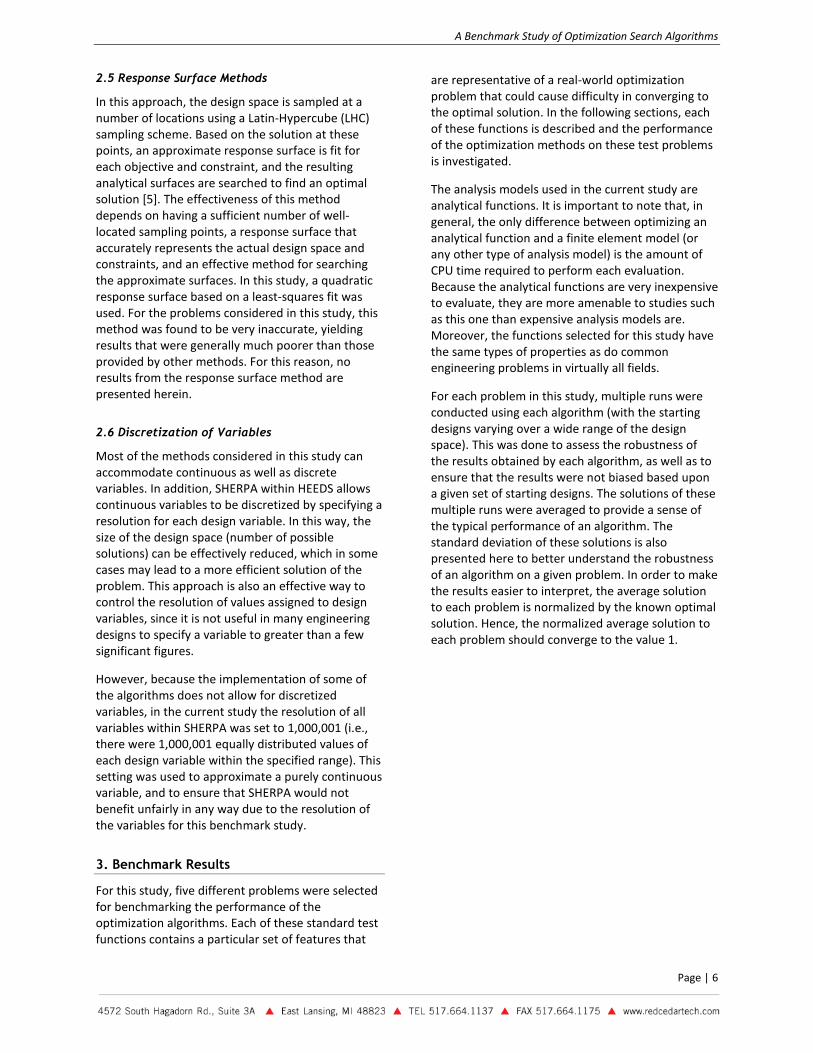
The Goldstein-Price Function has two variables and is slightly multi-modal and continuous. This function is defined as:

))273648123218(*)32(30(*))361431419(*)1(1( 22212

211

221

22212

211

221 xxxxxxxxxxxxxxxxf +−++−−+++−+−+++=

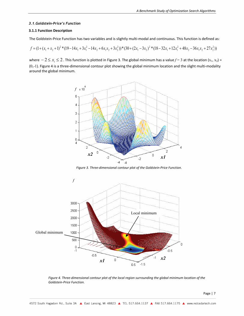
where 22 ≤≤− ix . This function is plotted in Figure 3. The global minimum has a value f = 3 at the location (x1, x2) =

(0,-1). Figure 4 is a three-dimensional contour plot showing the global minimum location and the slight multi-modality around the global minimum.

Figure 3. Three-dimensional contour plot of the Goldstein-Price Function.

Figure 4. Three-dimensional contour plot of the local region surrounding the global minimum location of the Goldstein-Price Function.

Local minimum

Global minimum

f

f

x2 x1

x2 x1


Page | 8

3.1.2 Results

This study was performed for five different values of the maximum number of evaluations: 100, 200, 500, 750 and 1000. A series of 50 runs was performed for each of the following optimization search methods: SHERPA, ASA, GA, and NLPQL.

As expected, NLPQL did not perform well on this multi-modal problem. Gradient-based methods are not able to explore more than one local minimum at a time, and they tend to get stuck in the nearest local minimum. While GA’s are very good at exploring multi-modal design spaces, they are often very inefficient at performing local search, which often slows their convergence rate considerably. Hence, the GA also did not perform well on this problem, as seen in Figure 5.

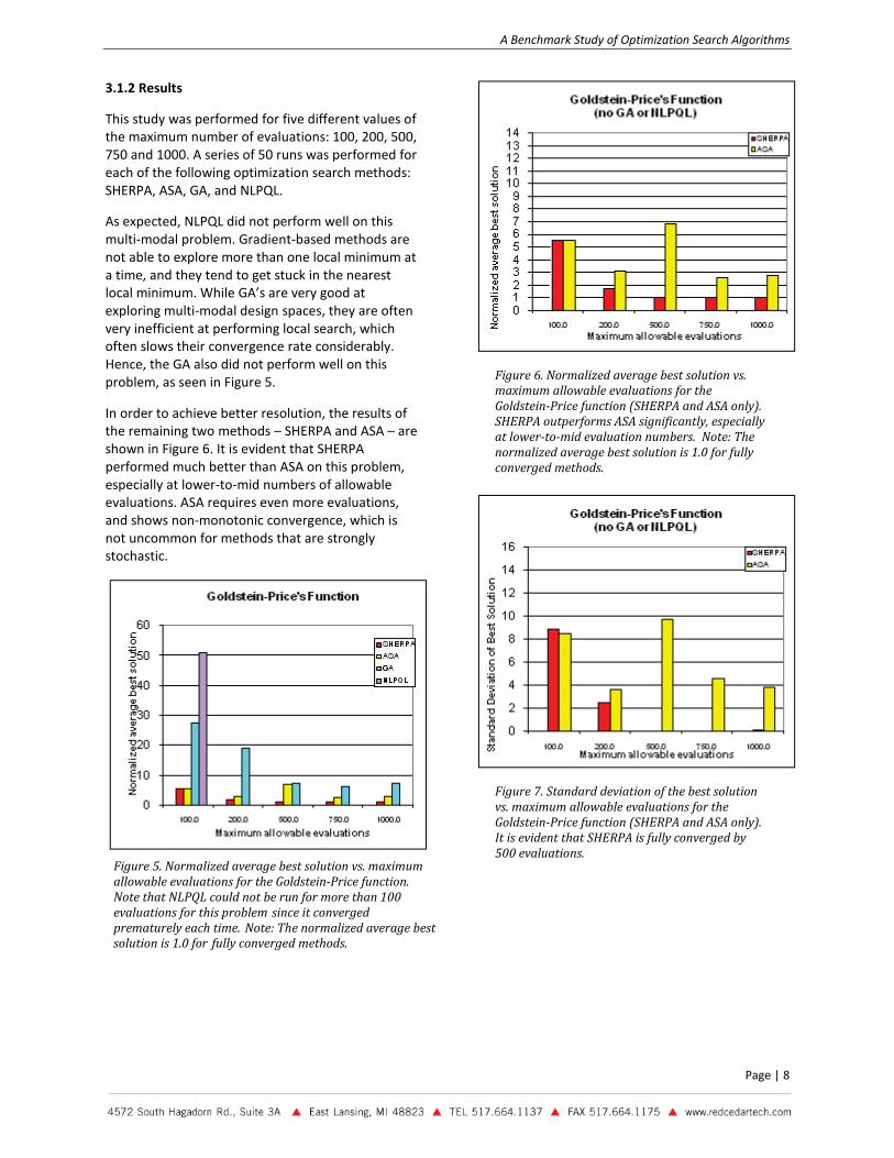
In order to achieve better resolution, the results of the remaining two methods – SHERPA and ASA – are shown in Figure 6. It is evident that SHERPA performed much better than ASA on this problem, especially at lower-to-mid numbers of allowable evaluations. ASA requires even more evaluations, and shows non-monotonic convergence, which is not uncommon for methods that are strongly stochastic.

Figure 6. Normalized average best solution vs. maximum allowable evaluations for the Goldstein-Price function (SHERPA and ASA only). SHERPA outperforms ASA significantly, especially at lower-to-mid evaluation numbers. Note: The normalized average best solution is 1.0 for fully converged methods.

Figure 7. Standard deviation of the best solution vs. maximum allowable evaluations for the Goldstein-Price function (SHERPA and ASA only). It is evident that SHERPA is fully converged by 500 evaluations.

Figure 5. Normalized average best solution vs. maximum allowable evaluations for the Goldstein-Price function. Note that NLPQL could not be run for more than 100 evaluations for this problem since it converged prematurely each time. Note: The normalized average best solution is 1.0 for fully converged methods.


Page | 9

3.2. Rosenbrock’s Valley


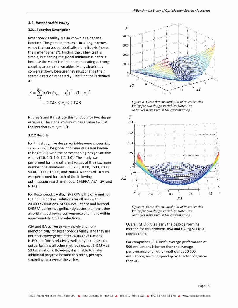
Rosenbrock’s Valley is also known as a banana function. The global optimum is in a long, narrow, valley that curves parabolically along its axis (hence the name “banana”). Finding the valley itself is simple, but finding the global minimum is difficult because the valley is non-linear, indicating a strong coupling among the variables. Many algorithms converge slowly because they must change their search direction repeatedly. This function is defined as:

21

1

221 )1()(100 i

n

iii xxxf −+−∗= ∑

−

=+

048.2048.2 ≤≤− ix

Figures 8 and 9 illustrate this function for two design variables. The global minimum has a value f = 0 at the location x1 = x2 = 1.0.

3.2.2 Results

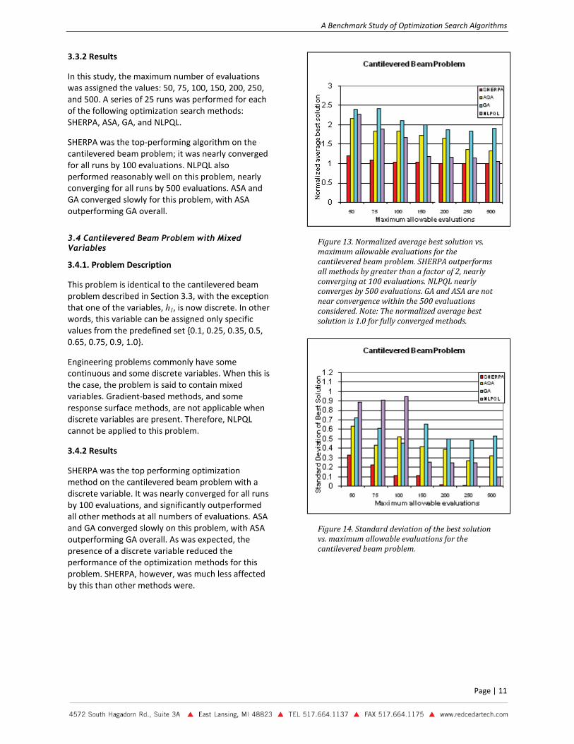
For this study, five design variables were chosen (x1, x2, x3, x4, x5). The global optimum value was known to be f = 0.0, with the corresponding design variable values (1.0, 1.0, 1.0, 1.0, 1.0). The study was performed for nine different values of the maximum number of evaluations: 500, 750, 1000, 1500, 2000, 5000, 10000, 15000, and 20000. A series of 10 runs was performed for each of the following optimization search methods: SHERPA, ASA, GA, and NLPQL.

For Rosenbrock’s Valley, SHERPA is the only method to find the optimal solutions for all runs within 20,000 evaluations. At 500 evaluations and beyond, SHERPA performs significantly better than the other algorithms, achieving convergence of all runs within approximately 1,500 evaluations.

ASA and GA converge very slowly and non-monotonically for Rosenbrock’s Valley, and they are not near convergence after 20,000 evaluations. NLPQL performs relatively well early in the search, outperforming all other methods except SHERPA at 500 evaluations. However, it is unable to make additional progress beyond this point, perhaps struggling to traverse the valley.

Figure 8. Three-dimensional plot of Rosenbrock’s Valley for two design variables. Note: Five variables were used in the current study.

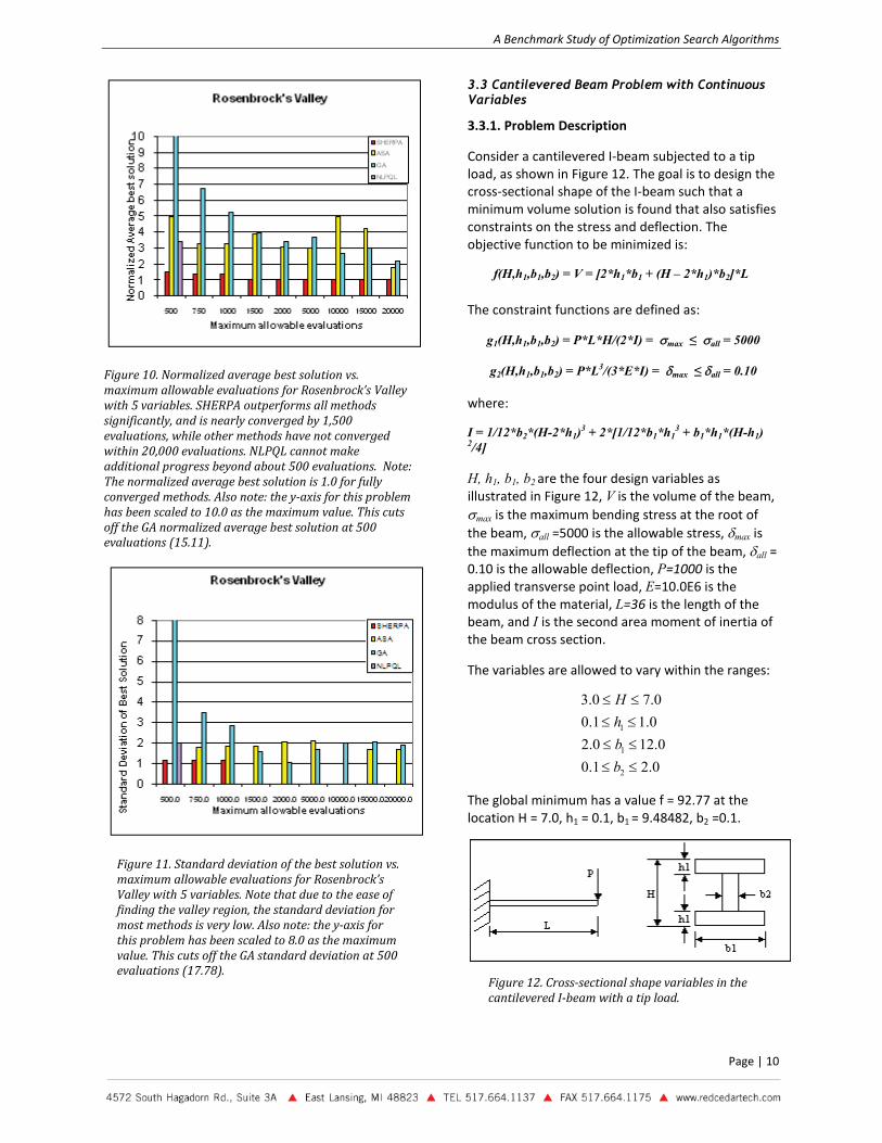
Figure 9. Three-dimensional plot of Rosenbrock’s Valley for two design variables. Note: Five variables were used in the current study.

Overall, SHERPA is clearly the best-performing method for this problem. ASA and GA lag SHERPA considerably.

For comparison, SHERPA’s average performance at 500 evaluations is better than the average performance of all other methods at 20,000 evaluations, yielding speedup by a factor of greater than 40.

x2 x1

f

x1

f

x2

x1


Page | 10

Figure 10. Normalized average best solution vs. maximum allowable evaluations for Rosenbrock’s Valley with 5 variables. SHERPA outperforms all methods significantly, and is nearly converged by 1,500 evaluations, while other methods have not converged within 20,000 evaluations. NLPQL cannot make additional progress beyond about 500 evaluations. Note: The normalized average best solution is 1.0 for fully converged methods. Also note: the y-axis for this problem has been scaled to 10.0 as the maximum value. This cuts off the GA normalized average best solution at 500 evaluations (15.11).

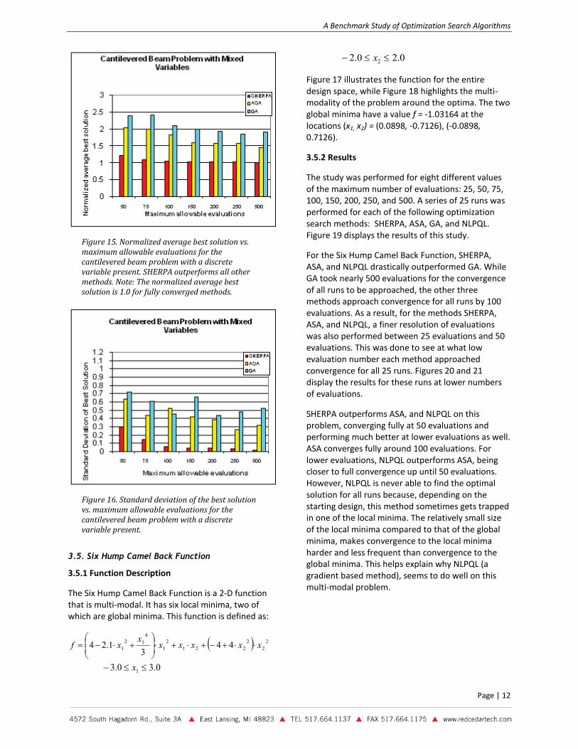
Figure 11. Standard deviation of the best solution vs. maximum allowable evaluations for Rosenbrock’s Valley with 5 variables. Note that due to the ease of finding the valley region, the standard deviation for most methods is very low. Also note: the y-axis for this problem has been scaled to 8.0 as the maximum value. This cuts off the GA standard deviation at 500 evaluations (17.78).

3.3 Cantilevered Beam Problem with Continuous Variables

3.3.1. Problem Description

Consider a cantilevered I-beam subjected to a tip load, as shown in Figure 12. The goal is to design the cross-sectional shape of the I-beam such that a minimum volume solution is found that also satisfies constraints on the stress and deflection. The objective function to be minimized is:

f(H,h1,b1,b2) = V = [2*h1*b1 + (H – 2*h1)*b2]*L

The constraint functions are defined as:

g1(H,h1,b1,b2) = P*L*H/(2*I) = σmax ≤ σall = 5000

g2(H,h1,b1,b2) = P*L3/(3*E*I) = δmax ≤ δall = 0.10

where:

I = 1/12*b2*(H-2*h1)3 + 2*[1/12*b1*h13 + b1*h1*(H-h1)

2/4] H, h1, b1, b2

are the four design variables as illustrated in Figure 12, V is the volume of the beam, σmax is the maximum bending stress at the root of the beam, σall =5000 is the allowable stress, δmax is the maximum deflection at the tip of the beam, δall = 0.10 is the allowable deflection, P=1000 is the applied transverse point load, E=10.0E6 is the modulus of the material, L=36 is the length of the beam, and I is the second area moment of inertia of the beam cross section.

The variables are allowed to vary within the ranges:

0.21.00.120.2

0.11.00.70.3

2

1

1

≤≤≤≤≤≤≤≤

bbhH

The global minimum has a value f = 92.77 at the location H = 7.0, h1 = 0.1, b1 = 9.48482, b2 =0.1.

Figure 12. Cross-sectional shape variables in the cantilevered I-beam with a tip load.


Page | 11

3.3.2 Results

In this study, the maximum number of evaluations was assigned the values: 50, 75, 100, 150, 200, 250, and 500. A series of 25 runs was performed for each of the following optimization search methods: SHERPA, ASA, GA, and NLPQL.

SHERPA was the top-performing algorithm on the cantilevered beam problem; it was nearly converged for all runs by 100 evaluations. NLPQL also performed reasonably well on this problem, nearly converging for all runs by 500 evaluations. ASA and GA converged slowly for this problem, with ASA outperforming GA overall.

3.4 Cantilevered Beam Problem with Mixed Variables

3.4.1. Problem Description

This problem is identical to the cantilevered beam problem described in Section 3.3, with the exception that one of the variables, h1, is now discrete. In other words, this variable can be assigned only specific values from the predefined set {0.1, 0.25, 0.35, 0.5, 0.65, 0.75, 0.9, 1.0}.

Engineering problems commonly have some continuous and some discrete variables. When this is the case, the problem is said to contain mixed variables. Gradient-based methods, and some response surface methods, are not applicable when discrete variables are present. Therefore, NLPQL cannot be applied to this problem.

3.4.2 Results

SHERPA was the top performing optimization method on the cantilevered beam problem with a discrete variable. It was nearly converged for all runs by 100 evaluations, and significantly outperformed all other methods at all numbers of evaluations. ASA and GA converged slowly on this problem, with ASA outperforming GA overall. As was expected, the presence of a discrete variable reduced the performance of the optimization methods for this problem. SHERPA, however, was much less affected by this than other methods were.

Figure 13. Normalized average best solution vs. maximum allowable evaluations for the cantilevered beam problem. SHERPA outperforms all methods by greater than a factor of 2, nearly converging at 100 evaluations. NLPQL nearly converges by 500 evaluations. GA and ASA are not near convergence within the 500 evaluations considered. Note: The normalized average best solution is 1.0 for fully converged methods.

Figure 14. Standard deviation of the best solution vs. maximum allowable evaluations for the cantilevered beam problem.


Page | 12

Figure 15. Normalized average best solution vs. maximum allowable evaluations for the cantilevered beam problem with a discrete variable present. SHERPA outperforms all other methods. Note: The normalized average best solution is 1.0 for fully converged methods.

Figure 16. Standard deviation of the best solution vs. maximum allowable evaluations for the cantilevered beam problem with a discrete variable present.

3.5. Six Hump Camel Back Function


The Six Hump Camel Back Function is a 2-D function that is multi-modal. It has six local minima, two of which are global minima. This function is defined as:

( ) 22

2221

21

412

1 443

1.24 xxxxxx

xf ⋅⋅+−+⋅+⋅

+⋅−=

0.30.3 1 ≤≤− x

0.20.2 2 ≤≤− x

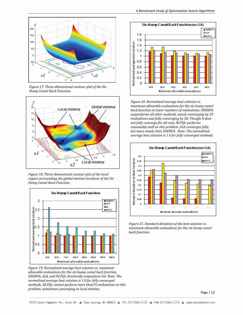
Figure 17 illustrates the function for the entire design space, while Figure 18 highlights the multi-modality of the problem around the optima. The two global minima have a value f = -1.03164 at the locations (x1, x2) = (0.0898, -0.7126), (-0.0898, 0.7126).

3.5.2 Results

The study was performed for eight different values of the maximum number of evaluations: 25, 50, 75, 100, 150, 200, 250, and 500. A series of 25 runs was performed for each of the following optimization search methods: SHERPA, ASA, GA, and NLPQL. Figure 19 displays the results of this study.

For the Six Hump Camel Back Function, SHERPA, ASA, and NLPQL drastically outperformed GA. While GA took nearly 500 evaluations for the convergence of all runs to be approached, the other three methods approach convergence for all runs by 100 evaluations. As a result, for the methods SHERPA, ASA, and NLPQL, a finer resolution of evaluations was also performed between 25 evaluations and 50 evaluations. This was done to see at what low evaluation number each method approached convergence for all 25 runs. Figures 20 and 21 display the results for these runs at lower numbers of evaluations.

SHERPA outperforms ASA, and NLPQL on this problem, converging fully at 50 evaluations and performing much better at lower evaluations as well. ASA converges fully around 100 evaluations. For lower evaluations, NLPQL outperforms ASA, being closer to full convergence up until 50 evaluations. However, NLPQL is never able to find the optimal solution for all runs because, depending on the starting design, this method sometimes gets trapped in one of the local minima. The relatively small size of the local minima compared to that of the global minima, makes convergence to the local minima harder and less frequent than convergence to the global minima. This helps explain why NLPQL (a gradient based method), seems to do well on this multi-modal problem.


Page | 13

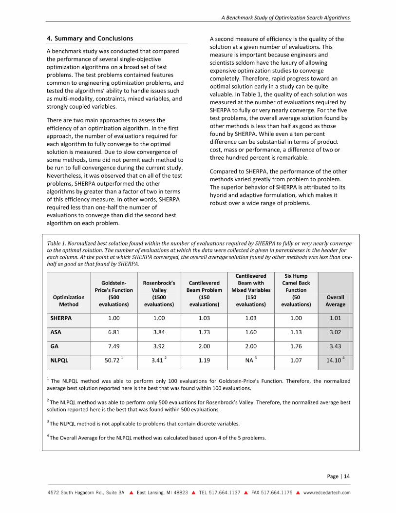
Figure 20. Normalized average best solution vs. maximum allowable evaluations for the six hump camel back function at lower numbers of evaluations. SHERPA outperforms all other methods, nearly converging by 35 evaluations and fully converging by 50. Though it does not fully converge for all runs, NLPQL performs reasonably well on this problem. ASA converges fully, but more slowly than SHERPA. Note: The normalized average best solution is 1.0 for fully converged methods.

Figure 21. Standard deviation of the best solution vs. maximum allowable evaluations for the six hump camel back function.

Figure 17. Three-dimensional contour plot of the Six Hump Camel Back Function.

Figure 19. Normalized average best solution vs. maximum allowable evaluations for the six-hump camel back function. SHERPA, ASA, and NLPQL drastically outperform GA. Note: The normalized average best solution is 1.0 for fully converged methods. NLPQL cannot perform more than75 evaluations on this problem, sometimes converging to local minima.

Figure 18. Three-dimensional contour plot of the local region surrounding the global minima locations of the Six Hump Camel Back Function.


Page | 14

4. Summary and Conclusions

A benchmark study was conducted that compared the performance of several single-objective optimization algorithms on a broad set of test problems. The test problems contained features common to engineering optimization problems, and tested the algorithms’ ability to handle issues such as multi-modality, constraints, mixed variables, and strongly coupled variables.

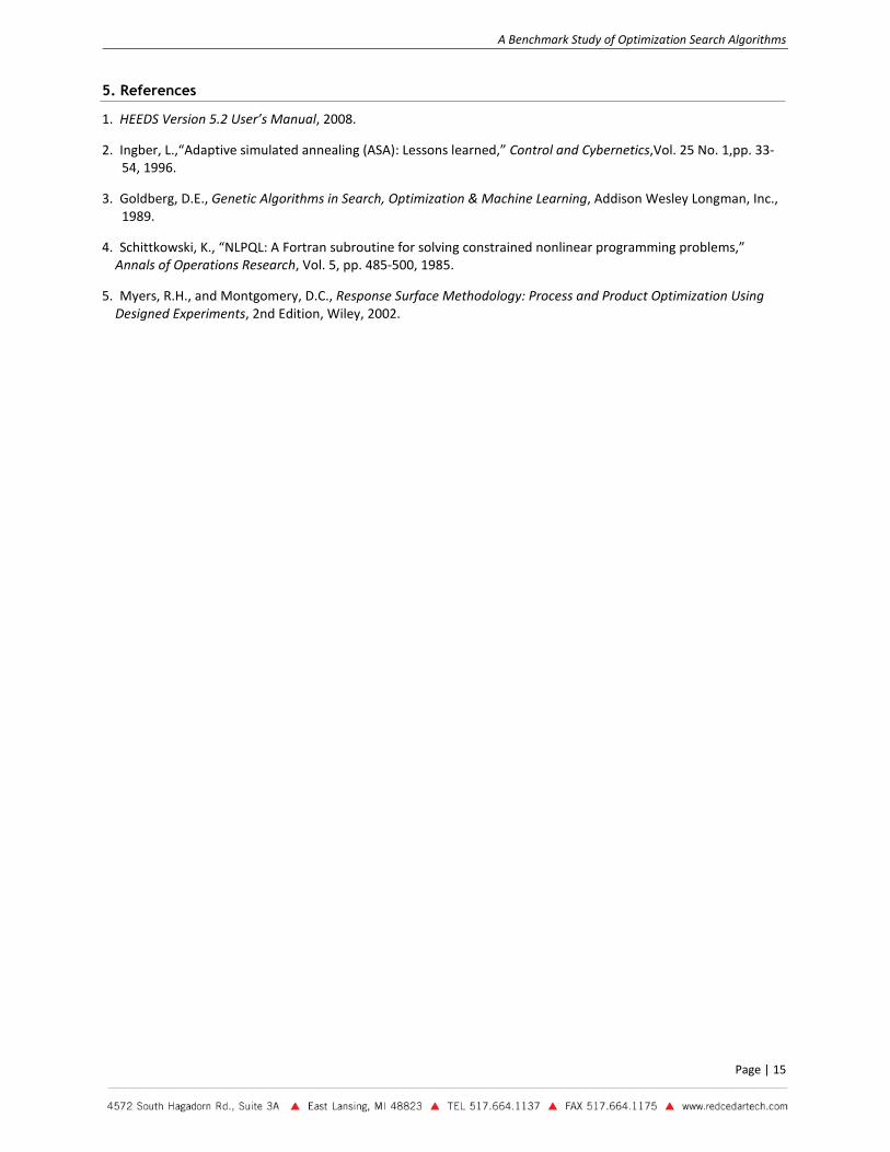
There are two main approaches to assess the efficiency of an optimization algorithm. In the first approach, the number of evaluations required for each algorithm to fully converge to the optimal solution is measured. Due to slow convergence of some methods, time did not permit each method to be run to full convergence during the current study. Nevertheless, it was observed that on all of the test problems, SHERPA outperformed the other algorithms by greater than a factor of two in terms of this efficiency measure. In other words, SHERPA required less than one-half the number of evaluations to converge than did the second best algorithm on each problem.

A second measure of efficiency is the quality of the solution at a given number of evaluations. This measure is important because engineers and scientists seldom have the luxury of allowing expensive optimization studies to converge completely. Therefore, rapid progress toward an optimal solution early in a study can be quite valuable. In Table 1, the quality of each solution was measured at the number of evaluations required by SHERPA to fully or very nearly converge. For the five test problems, the overall average solution found by other methods is less than half as good as those found by SHERPA. While even a ten percent difference can be substantial in terms of product cost, mass or performance, a difference of two or three hundred percent is remarkable.

Compared to SHERPA, the performance of the other methods varied greatly from problem to problem. The superior behavior of SHERPA is attributed to its hybrid and adaptive formulation, which makes it robust over a wide range of problems.

Optimization Method

Goldstein-Price’s Function

(500 evaluations)

Rosenbrock’s Valley (1500

evaluations)

Cantilevered Beam Problem

(150 evaluations)

Cantilevered Beam with

Mixed Variables (150

evaluations)

Six Hump Camel Back

Function (50

evaluations) Overall Average

SHERPA 1.00 1.00 1.03 1.03 1.00 1.01

ASA 6.81 3.84 1.73 1.60 1.13 3.02

GA 7.49 3.92 2.00 2.00 1.76 3.43

NLPQL 50.72 1 3.41 2 1.19 NA 3 1.07 14.10 4

1 The NLPQL method was able to perform only 100 evaluations for Goldstein-Price’s Function. Therefore, the normalized average best solution reported here is the best that was found within 100 evaluations. 2 The NLPQL method was able to perform only 500 evaluations for Rosenbrock’s Valley. Therefore, the normalized average best solution reported here is the best that was found within 500 evaluations. 3 The NLPQL method is not applicable to problems that contain discrete variables. 4 The Overall Average for the NLPQL method was calculated based upon 4 of the 5 problems.

Table 1. Normalized best solution found within the number of evaluations required by SHERPA to fully or very nearly converge to the optimal solution. The number of evaluations at which the data were collected is given in parentheses in the header for each column. At the point at which SHERPA converged, the overall average solution found by other methods was less than one-half as good as that found by SHERPA.


Page | 15

5. References

1. HEEDS Version 5.2 User’s Manual, 2008.

2. Ingber, L.,“Adaptive simulated annealing (ASA): Lessons learned,” Control and Cybernetics,Vol. 25 No. 1,pp. 33-54, 1996.

3. Goldberg, D.E., Genetic Algorithms in Search, Optimization & Machine Learning, Addison Wesley Longman, Inc., 1989.

4. Schittkowski, K., “NLPQL: A Fortran subroutine for solving constrained nonlinear programming problems,” Annals of Operations Research, Vol. 5, pp. 485-500, 1985.

5. Myers, R.H., and Montgomery, D.C., Response Surface Methodology: Process and Product Optimization Using Designed Experiments, 2nd Edition, Wiley, 2002.

http://www.ingber.com/asa96_lessons.ps.gz�

a benchmark study of optimization search algorithms rev. 01.10 a benchmark study of optimization...

Documents