a 3-approximation algorithm for the facility location problem with uniform capacities

Math. Program., Ser. A (2013) 141:527–547DOI 10.1007/s10107-012-0565-4

FULL LENGTH PAPER

A 3-approximation algorithm for the facility locationproblem with uniform capacities

Ankit Aggarwal · Anand Louis · Manisha Bansal ·Naveen Garg · Neelima Gupta · Shubham Gupta ·Surabhi Jain

Received: 28 July 2010 / Accepted: 25 April 2012 / Published online: 9 June 2012© Springer and Mathematical Optimization Society 2012

Abstract We consider the facility location problem where each facility can serve atmost U clients. We analyze a local search algorithm for this problem which uses onlythe operations of add, delete and swap and prove that any locally optimum solutionis no more than 3 times the global optimum. This improves on a result of Chudak andWilliamson who proved an approximation ratio of 3 + 2

√2 for the same algorithm.

We also provide an example which shows that any local search algorithm which usesonly these three operations cannot achieve an approximation guarantee better than 3.

Keywords Facility location · Local search · Approximation algorithms ·Uniform capacities

Work done as part of the “Approximation Algorithms” partner group of MPI-Informatik, Germany.

A. AggarwalTower Research Capital LLC, Gurgaon, India

A. LouisGeorgia Tech, Atlanta, GA, USA

M. Bansal · N. GuptaUniversity of Delhi, Delhi, India

N. Garg (B)Indian Institute of Technology Delhi, Delhi, Indiae-mail: [email protected]

S. GuptaGoogle, Mountain View, CA, USA

S. JainGoogle, London, UK

123

528 A. Aggarwal et al.

Mathematics Subject Classification (2000) 90B80 · 90C59 · 68W25 · 68W40 ·68Q25

1 Introduction

In a facility location problem we are given a set of clients C and facility locations F .Opening a facility at location i ∈ F costs fi (the facility cost). The cost of servicing aclient j by a facility i is given by ci, j (the service cost) and these costs form a metrici.e. for facilities i, i ′ and clients j, j ′, ci ′, j ′ ≤ ci ′, j + ci, j + ci, j ′ . The objective is todetermine which locations to open facilities in, so that the total cost for opening thefacilities and for serving all the clients is minimized. Note that in this setting eachclient would be served by the open facility which offers the smallest service cost.

When the number of clients that a facility can serve is bounded, we have a capac-itated facility location problem. In this paper we assume that these capacities are thesame, U , for all facilities. For this problem of uniform capacities the first approxi-mation algorithm was due to Korupolu et al. [4] who analyzed a local search algo-rithm and proved that any locally optimum solution has cost no more than 8 timesthe facility cost plus 5 times the service cost of an (global) optimum solution. In thispaper we refer to such a guarantee as a (8,5)-approximation; note that this is differ-ent from the bi-criterion guarantees for which this notation is typically used. Chudakand Williamson [3] strengthened the analysis in [4] to obtain a (6,5)-approximation.Charikar and Guha [2] gave a general technique for scaling facility costs that improvesthe approximation guarantee to 3+ 2

√2.

Given the set of open facilities, the best way of serving the clients, can be deter-mined by solving an assignment problem. Thus any solution is completely determinedby the set of open facilities. The local search procedure proposed by Korupolu et al.starts with an arbitrary set of open facilities and then updates this set, using one ofthe operations add, delete, swap, whenever that operation reduces the total costof the solution. We show that a solution which is locally optimum with respect to thissame set of operations is a (3,3)-approximation. We then show that our analysis of thislocal search algorithm is best possible by demonstrating an instance where the locallyoptimum solution is 3 times the (global) optimum solution.

When facilities have different capacities, the best result known is a (6,5)-approxi-mation by Zhang et al. [8]. The local search in this case relies on a multi-exchangeoperation, in which, loosely speaking, a subset of facilities from the current solution isexchanged with a subset not in the solution. This result improves on a (8,7)-approxi-mation by Mahdian and Pal [5] and a (9,5) approximation by Pal et al. [7].

For capacitated facility location, the only algorithms known are based on localsearch. One version of capacitated facility location arises when we are allowed tomake multiple copies of the facilities. Thus if facility i has capacity Ui and openingcost fi , then to serve k > Ui clients by facility i we need to open �k/Ui� copies ofi and incur an opening cost fi�k/Ui�. This version is usually referred to as “facil-ity location with soft capacities” and the best known algorithm for this problem is a2-approximation [6].

123

Facility location with uniform capacities 529

All earlier work for capacitated facility location (uniform or non-uniform) reroutesall clients in a swap operation from the facility which is closing to one of the facilitiesbeing opened. This however can be quite expensive and cannot lead to the tight boundsthat we achieve in this paper. We use the idea of Arya et al. [1] to reassign some cli-ents of the facility being closed in a swap operation to other facilities in our currentsolution. However, to be able to handle the capacity constraints in this reassignmentwe need to extend the notion of the mapping between clients used in [1] to a fractionalassignment. As in earlier work, we use the fact that when we have a local optimum, nooperation leads to an improvement in cost. However, we now take carefully definedlinear combinations of the inequalities capturing this local optimality. All previouswork that we are aware of seems to only use the sum of such inequalities and thereforerequires additional properties like the integrality of the assignment polytope to iden-tify suitable swaps [3]. Our approach is therefore more general and amenable to betteranalysis. The idea of doing things fractionally appears more often in our analysis.Thus, when analyzing the cost of an operation we assign clients fractionally to thefacilities and rely on the fact that such a fractional assignment cannot be better than theoptimum assignment which follows from the integrality of the assignment polytope.

In Sect. 5 we give a tight example that requires the construction of a suitable set-system. While this construction itself is quite straightforward, this is the first instancewe know of where such an idea has been applied to prove a large locality gap.

2 Preliminaries

Let C be the set of clients and F denote the facility locations. Let S (resp. O) bethe set of open facilities in our solution (resp. optimum solution). We abuse notationand use S (resp. O) to denote our solution (resp. optimum solution). Initially S is anarbitrary set of facilities which can serve all the clients. Let cost(S) denote the totalcost (facility plus service) of solution S. The three operations that make up our localsearch algorithm are

Add For s /∈ S, if cost(S + {s}) < cost(S) then S← S + {s}.Delete For s ∈ S, if cost(S − {s}) < cost(S) then S← S − {s}.Swap For s ∈ S and s′ /∈ S, if cost(S − {s} + {s′}) < cost(S) then S← S − {s} +

{s′}.S is locally optimum if none of the three operations are possible and at this point ouralgorithm stops.

We use fi , i ∈ F to denote the cost of opening a facility at location i . Let S j , O j

denote the service-cost of client j in the solutions S and O , respectively. The presenceof the add operation ensures that the total service cost of the clients in any locallyoptimum solution is at most the total cost of the optimum solution [4]. Formally,

Lemma 1 ([4]) For any locally optimum solution S,∑

j∈C S j ≤ ∑j∈C O j +∑

o∈O fo.

We reprove this Lemma in Sect. 4.Hence, most of the effort in this paper is towards bounding the facility cost of

a locally optimum solution which we show is no more than 2 times the cost of an

123


optimum solution. We prove this by identifying a suitable set of local operations anddetermine the increase in cost if these operations were to be performed. Since thesolution is locally optimum, the increase in cost due to these operations is non-neg-ative.1 This gives us a set of inequalities and a suitable linear combination of theseinequalities yields the bound on the facility cost of the locally optimum solution. Notethat the inequalities generated are only for the purpose of analysis; we do not actuallyperform those local operations since we are already at a locally optimum solution.

Combining the bounds of the service cost and the facility cost of a locally optimumsolution then gives us our main theorem.

Theorem 1 For any locally optimum solution S and an optimum solution O to thefacility location problem with uniform capacities, cost(S) ≤ 3cost(O).

To ensure that our procedure has a polynomial running time we use an idea firstproposed in [4]—a local step is performed only if the cost of the solution reduces bymore than (ε/4n)cost(S) where ε > 0 and n = |F | is the number of facility loca-tions. It is immediate that as a result of this modification the number of local searchsteps done is at most 4nε−1 log(cost(S0)/cost(O)) where S0 is the initial solution. InSect. 3 we argue the approximation guarantee of this modified local search procedureincreases to at most 3/(1− ε).

The rest of the paper is organized as follows. In Sect. 3 we bound the facility costsof the locally optimum solution assuming that the facilities in the locally optimumsolution, S are disjoint from the facilities of the optimum solution, O . Most of thenew ideas in the paper appear in this section. In Sect. 4 we extend the argument to thecase when the facilities in S and O are not disjoint. In Sect. 5 we give an example of asolution which is locally optimal with respect to the operations of add, delete,swap and has cost three times the optimum. This establishes that our analysis is tight.

3 Bounding the facility costs

Let S denote the locally optimum solution obtained. For the rest of this section weassume that the sets S and O are disjoint. This assumption allows us to add any facil-ity of O or to swap any facility in S with a facility in O without worrying about thepossibility that the facility of O included in our solution might already be part of S.

Let NS(s) denote the clients served by facility s in the solution S and NO(o) denotethe clients served by facility o in solution O . Let N o

s denote the set of clients servedby facility s in solution S and by facility o in solution O . We will associate a weight,wt : C → [0..1], with each client which satisfies the following properties.

1. For a client j ∈ C let σ( j) be the facility which serves j in solution S. Then

wt( j) ≤ min

(

1,U − |NS(σ ( j))||NS(σ ( j))|

)

.

1 In fact, we do not determine the exact increase in cost when a local operation is performed but only anupperbound on this quantity.

123


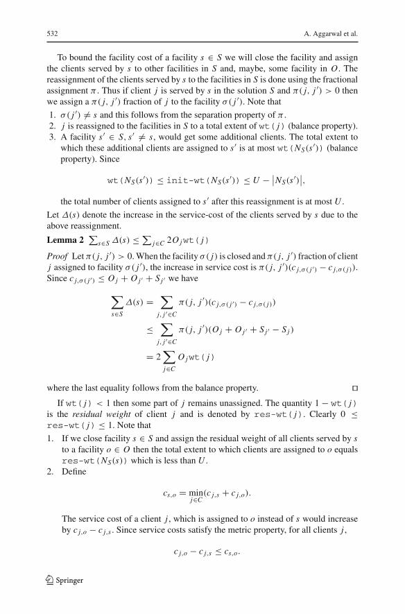
Fig. 1 Defining πo. The lower arrangement is obtained by splitting the top arrangement at the centraldotted line and swapping the two halves

Let init-wt( j) denote the quantity on the right of the above inequality. Since|NS(σ ( j))| ≤ U , we have that 0 ≤ init-wt( j) ≤ 1.

2. For all o ∈ O and s ∈ S, wt(N os ) ≤ wt(NO(o))/2. Here for X ⊆ C , wt(X)

denotes the sum of the weights of the clients in X .

To determine wt( j) so that these two properties are satisfied we start by assign-ing wt( j) = init-wt( j). However, this assignment might violate the sec-ond property. A facility s ∈ S captures a facility o ∈ O if init-wt(N o

s ) >

init-wt(NO(o))/2. Note that at most one facility in S can capture a facility o. Ifs does not capture o then for all j ∈ N o

s define wt( j) = init-wt( j). However ifs captures o then for all j ∈ N o

s define wt( j) = α · init-wt( j) where α < 1 issuch that wt(N o

s ) = wt(NO(o))/2. Note that if N os = NO(o) then α = 0.

For a facility o ∈ O we define a fractional assignment πo : NO(o)×NO(o)→ �+with the following properties.

separation πo( j, j ′) > 0 only if j and j ′ are served by different facilities in S.balance

∑j ′∈NO (o) πo( j ′, j) = ∑

j ′∈NO (o) πo( j, j ′) = wt( j) for all j ∈NO(o).

The fractional assignment πo can be obtained along the same lines as the map-ping in [1]. Associate an interval of length wt( j) for each j ∈ NO(o) and arrangethese intervals on a line segment of length wt(NO(o)) (see Fig. 1). The intervalsare ordered so that intervals corresponding to clients served by the same facility in Sappear together. Consider another arrangement of intervals obtained from the first bysplitting the line segment at the center and swapping the two halves. As a consequence,one interval might be split and be non-contiguous in the second arrangement. Super-impose these two arrangements. πo( j, j ′) is now defined as the overlap between theinterval corresponding to j in the first arrangement and the interval j ′ in the second.The second property of the weights ensures that there is no overlap between an inter-val in the first arrangement and the corresponding interval in the second arrangement.Further, it is easy to see that the mapping πo as defined here satisfies the properties ofseparation and balance.

The individual fractional assignments πo are extended to a fractional assignmentover all clients, π : C × C → �+ in the obvious way—π( j, j ′) = πo( j, j ′) ifj, j ′ ∈ NO(o) and is 0 otherwise.

123


To bound the facility cost of a facility s ∈ S we will close the facility and assignthe clients served by s to other facilities in S and, maybe, some facility in O . Thereassignment of the clients served by s to the facilities in S is done using the fractionalassignment π . Thus if client j is served by s in the solution S and π( j, j ′) > 0 thenwe assign a π( j, j ′) fraction of j to the facility σ( j ′). Note that

1. σ( j ′) �= s and this follows from the separation property of π .2. j is reassigned to the facilities in S to a total extent of wt( j) (balance property).3. A facility s′ ∈ S, s′ �= s, would get some additional clients. The total extent to

which these additional clients are assigned to s′ is at most wt(NS(s′)) (balanceproperty). Since

wt(NS(s′)) ≤ init-wt(NS(s′)) ≤ U − ∣∣NS(s′)

∣∣,

the total number of clients assigned to s′ after this reassignment is at most U .

Let Δ(s) denote the increase in the service-cost of the clients served by s due to theabove reassignment.

Lemma 2∑

s∈S Δ(s) ≤∑j∈C 2O jwt( j)

Proof Let π( j, j ′) > 0. When the facility σ( j) is closed and π( j, j ′) fraction of clientj assigned to facility σ( j ′), the increase in service cost is π( j, j ′)(c j,σ ( j ′) − c j,σ ( j)).Since c j,σ ( j ′) ≤ O j + O j ′ + S j ′ we have

∑

s∈S

Δ(s) =∑

j, j ′∈C

π( j, j ′)(c j,σ ( j ′) − c j,σ ( j))

≤∑

j, j ′∈C

π( j, j ′)(O j + O j ′ + S j ′ − S j )

= 2∑

j∈C

O jwt( j)

where the last equality follows from the balance property. �If wt( j) < 1 then some part of j remains unassigned. The quantity 1 − wt( j)

is the residual weight of client j and is denoted by res-wt( j). Clearly 0 ≤res-wt( j) ≤ 1. Note that

1. If we close facility s ∈ S and assign the residual weight of all clients served by sto a facility o ∈ O then the total extent to which clients are assigned to o equalsres-wt(NS(s)) which is less than U .

2. Define

cs,o = minj∈C

(c j,s + c j,o).

The service cost of a client j , which is assigned to o instead of s would increaseby c j,o − c j,s . Since service costs satisfy the metric property, for all clients j ,

c j,o − c j,s ≤ cs,o.

123


3. The total increase in service cost of all clients in NS(s) which are assigned (partly)to o is at most cs,ores-wt(NS(s)).

Let 〈s, o〉 denote the swapping of facilities s, o and the reassignment of clientsserved by s to facilities in S−{s}∪{o} as discussed above. Since S is locally optimumwe have

fo − fs + cs,ores-wt(NS(s))+Δ(s) ≥ 0. (1)

The above inequalities are written for every pair (s, o), s ∈ S, o ∈ O . We take a linearcombination of these inequalities with the inequality corresponding to 〈s, o〉 having aweight λs,o in the combination to get∑

s,o

λs,o fo −∑

s,o

λs,o fs +∑

s,o

λs,ocs,ores-wt(NS(s))+∑

s,o

λs,oΔ(s) ≥ 0. (2)

where

λs,o = res-wt(N os )

res-wt(NS(s))

and is 0 if res-wt(NS(s)) = 0. Let S′ be the subset of facilities in the solution S forwhich res-wt(NS(s)) = 0. A facility s ∈ S′ can be deleted from S and its clientsreassigned completely to the other facilities in S. This implies

− fs +Δ(s) ≥ 0 (3)

We write such an inequality for each s ∈ S′ and add them to inequality (2).Note that for all s ∈ S − S′,

∑o λs,o = 1. This implies that

∑

s∈S′fs +

∑

s,o

λs,o fs =∑

s

fs (4)

and∑

s∈S′Δ(s)+

∑

s,o

λs,oΔ(s) =∑

s

Δ(s) ≤∑

j∈C

2O jwt( j) (5)

However, the reason for defining λs,o as above is to ensure the following property.

Lemma 3∑

s,o λs,ocs,ores-wt(NS(s)) ≤∑j∈C res-wt( j)(O j + S j )

Proof The left hand side in the inequality is∑

s,o cs,ores-wt(N os ). Since for each

client j ∈ N os , cs,o ≤ O j + S j we have

cs,ores-wt(N os ) =

∑

j∈N os

cs,ores-wt( j)

≤∑

j∈N os

res-wt( j)(O j + S j )

which, when summed over all s and o implies the Lemma. �

123


Incorporating equations (4), (5) and Lemma 3 into inequality (2) we get

∑

s

fs ≤∑

s,o

λs,o fo +∑

j∈C

res-wt( j)(O j + S j )+∑

j∈C

2O jwt( j)

=∑

s,o

λs,o fo + 2∑

j∈C

O j +∑

j∈C

res-wt( j)(S j − O j ) (6)

We now need to bound the number of times a facility of the optimum solution may beopened.

Lemma 4 For all o ∈ O,∑

s λs,o ≤ 2.

Proof We begin with the following observations.

1. For all s, o, λs,o ≤ 1.2. Let I ⊆ S be the facilities s such that s does not capture o and |NS(s)| ≤

U/2. Let s ∈ I and j ∈ N os . Note that wt( j) = init-wt( j) = 1 and so

res-wt( j) = 0. This implies that res-wt(N os ) = 0 and so for all s ∈ I ,

λs,o = 0.

Thus we only need to show that∑

s /∈I λs,o ≤ 2. We now consider two cases.

1. o is not captured by any s ∈ S. Let s be a facility not in I which does not captureo. For j ∈ N o

s ,

res-wt( j) = 1− wt( j) = 1− init-wt( j) = 2− U

|NS(s)| .

However, for j ∈ NS(s) we have that

res-wt( j) = 1− wt( j) ≥ 1− init-wt( j) = 2− U

|NS(s)| .

Therefore

λs,o ≤∣∣N o

s

∣∣

|NS(s)|Hence

∑

s

λs,o =∑

s /∈I

λs,o ≤∑

s /∈I

∣∣N o

s

∣∣

|NS(s)| ≤∑

s /∈I

∣∣N o

s

∣∣

U/2≤ |NO(o)|

U/2≤ 2.

2. o is captured by s′ ∈ S. This implies

init-wt(N os′) ≥

∑

s �=s′init-wt(N o

s )

≥∑

s /∈I∪{s′}init-wt(N o

s )

123


=∑

s /∈I∪{s′}

∣∣N o

s

∣∣U − |NS(s)||NS(s)|

=∑

s /∈I∪{s′}

(

U

∣∣N o

s

∣∣

|NS(s)| −∣∣N o

s

∣∣

)

Since init-wt(N os′) ≤

∣∣N o

s′∣∣ rearranging we get,

∑

s /∈I∪{s′}

∣∣N o

s

∣∣

|NS(s)| ≤∑

s /∈I

∣∣N o

s

∣∣

U≤ 1.

Now

∑

s /∈I∪{s′}λs,o ≤

∑

s /∈I∪{s′}

∣∣N o

s

∣∣

|NS(s)| ≤ 1

and since λs′,o ≤ 1 we have

∑

s

λs,o =∑

s /∈I

λs,o ≤ 2.

This completes the proof. �Incorporating Lemma 4 into inequality (6) we get

∑

s

fs ≤ 2

⎛

⎝∑

o

fo +∑

j∈C

O j

⎞

⎠+∑

j∈C

res-wt( j)(S j − O j ) (7)

Note that∑

j∈C res-wt( j)(S j −O j ) is at most∑

j∈C (S j −O j ) which in turn canbe bounded by

∑o fo by considering the operation of adding facilities in the optimum

solution. This, however, would lead to a bound of 3∑

o fo+2∑

j∈C O j on the facilitycost of our solution.

The key to obtaining a sharper bound on the facility cost of our solution is theobservation that in the swap 〈s, o〉 facility o gets only res-wt(NS(s)) clients andso can accommodate an additional U − res-wt(NS(s)) clients. Since we need tobound

∑j∈C res-wt( j)(S j − O j ), we assign the clients in NO(o) to facility o

in the ratio of their residual weights. Thus client j would be assigned to an extentβs,ores-wt( j) where

βs,o = min

(

1,U − res-wt(NS(s))

res-wt(NO(o))

)

.

βs,o is defined so that o gets at most U clients. Let Δ′(s, o) denote the increase inservice cost of the clients of NO(o) due to this reassignment. Hence

123


Δ′(s, o) = βs,o

∑

j∈NO (o)

res-wt( j)(O j − S j ). (8)

The inequality (1) corresponding to the swap 〈s, o〉 would now get an additional termΔ′(s, o) on the left. Hence the term

∑s,o λs,oΔ

′(s, o) would appear on the left ininequality (2) and on the right in inequality (6).

Now

∑

s

λs,oΔ′(s, o) =

∑

s

⎛

⎝λs,oβs,o

∑

j∈NO (o)

res-wt( j)(O j − S j )

⎞

⎠

=(

∑

s

λs,oβs,o

)∑

j∈NO (o)

res-wt( j)(O j − S j ).

If∑

s λs,oβs,o > 1 then we reduce some βs,o so that the sum is exactly 1 (we will latershow that this does not affect the analysis). On the other hand if

∑s λs,oβs,o = 1−γo,

γo > 0, then we take the inequalities corresponding to the operation of adding thefacility o ∈ O

fo +∑

j∈NO (o)

res-wt( j)(O j − S j ) ≥ 0 (9)

and add these to inequality (2) with a weight γo. Hence the total increase in the lefthand side of inequality (2) is

∑

s,o

λs,oΔ′(s, o)+

∑

o

γo

⎛

⎝ fo +∑

j∈NO (o)


⎞

⎠

=∑

o

∑

j∈NO (o)

(1− γo)res-wt( j)(O j − S j )

+∑

o

γo fo +∑

o

∑

j∈NO (o)

γores-wt( j)(O j − S j )

=∑

o

∑

j∈NO (o)

res-wt( j)(O j − S j )+∑

o

γo fo

=∑

j∈C

res-wt( j)(O j − S j )+∑

o

γo fo

and so inequality (6) now becomes

∑

s

fs ≤∑

o

∑

s

λs,o fo + 2∑

j∈C

O j +∑

o

γo fo

+∑

j∈C

res-wt( j)(S j − O j )+∑

j∈C


123


=∑

o

(

γo +∑

s

λs,o

)

fo + 2∑

j∈C

O j

=∑

o

(

1+∑

s

λs,o(1− βs,o)

)

fo + 2∑

j∈C

O j

≤ 2

⎛

⎝∑

o

fo +∑

j∈C

O j

⎞

⎠

where the last inequality follows from the following Lemma.

Lemma 5∑

s λs,o(1− βs,o) ≤ 1.

Proof When∑

s λs,oβs,o > 1 we reduced some βs,o to ensure that the sum is exactly1. In this case

∑

s

λs,o(1− βs,o) =∑

s

λs,o − 1 ≤ 1,

since by Lemma 4,∑

s λs,o ≤ 2.We now assume that no βs,o was reduced. Since

res-wt(NO(o)) ≤ |NO(o)| ≤ U

we have

βs,o = min

(

1,U − res-wt(NS(s))

res-wt(NO(o))

)

≥ min

(

1, 1− res-wt(NS(s))

res-wt(NO(o))

)

= 1− res-wt(NS(s))

res-wt(NO(o))

Hence

∑

s

λs,o(1− βs,o) ≤∑

s

res-wt(N os )

res-wt(NO(o))= 1.

�

This completes the proof of the following theorem.

Theorem 2 When S ∩ O = φ, the total cost of open facilities in any locally optimumsolution is at most twice the cost of an optimum solution.

123


Recall that to ensure that the local search procedure has a polynomial running timewe modified the local search procedure so that a step was performed only when thecost of the solution decreases by at least (ε/4n)cost(S). This modification impliesthat the right hand sides of inequalities (1), (3) and (9) which are all zero shouldinstead be (−ε/4n)cost(S). Note that for every choice of s ∈ S and o ∈ O we adda λs,o multiple of inequality (1) to obtain inequality (2). Since

∑o λs,o = 1, hence∑

o,s λs,o = |S| ≤ n. We also add inequality (3) for every s ∈ S to inequality (2).Similarly, for every o ∈ O , a γo (γo ≤ 1) multiple of inequality (9) is added toinequality (2).

Putting all these modifications together gives rise to an extra term of at most(3ε/4)cost(S). This implies that the facility cost of solution S is at most 2cost(O) +(3ε/4)cost(S). Similarly, the service cost of solution S can now be bounded bycost(O)+ (ε/4)cost(S). Adding these yields

(1− ε)cost(S) ≤ 3cost(O)

which implies that S is a 3/(1− ε) approximation to the optimum solution.

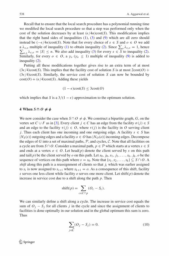
4 When S ∩ O �= φ

We now consider the case when S ∩ O �= φ. We construct a bipartite graph, G, on thevertex set C ∪ F as in [3]. Every client j ∈ C has an edge from the facility σ( j) ∈ Sand an edge to the facility τ( j) ∈ O , where τ( j) is the facility in O serving clientj . Thus each client has one incoming and one outgoing edge. A facility s ∈ S has|NS(s)| outgoing edges and a facility o ∈ O has |NO(o)| incoming edges. Decomposethe edges of G into a set of maximal paths, P , and cycles, C. Note that all facilities ona cycle are from S∩O . Consider a maximal path, p ∈ P which starts at a vertex s ∈ Sand ends at a vertex o ∈ O . Let head(p) denote the client served by s on this pathand tail(p) be the client served by o on this path. Let s0, j0, s1, j1, . . . , sk, jk, o be thesequence of vertices on this path where s = s0. Note that {s1, s2, . . . , sk} ⊆ S ∩ O . Ashift along this path is a reassignment of clients so that ji which was earlier assignedto si is now assigned to si+1 where sk+1 = o. As a consequence of this shift, facilitys serves one less client while facility o serves one more client. Let shift(p) denote theincrease in service cost due to a shift along the path p. Then

shift(p) =∑

c∈C∩p

(Oc − Sc).

We can similarly define a shift along a cycle. The increase in service cost equals thesum of O j − S j for all clients j in the cycle and since the assignment of clients tofacilities is done optimally in our solution and in the global optimum this sum is zero.Thus

∑

j∈C(O j − S j ) = 0. (10)

123


Fig. 2 An instance showing the decomposition into cycles (dotted arcs), swap paths (solid arcs) and trans-fer paths (dashed arcs). The facilities labeled so1, so2, so3 and so4 are in S ∩ O and have been duplicated.The cycle is so1, so2, so3, so1. The transfer paths are (s1, so2, so1), (s2, so2) and (s2, so3). The swappaths are s1, so1, so3, o1 and s2, so4, o1

Consider the operation of adding a facility o ∈ O . We shift along all paths whichend at o. The increase in service cost due to these shifts equals the sum of O j − S j

for all clients j on these paths and this quantity is at least − fo.∑

j∈P(O j − S j ) ≥ −

∑

o∈O

fo. (11)

Thus∑

j∈C

(O j − S j ) =∑

j∈P(O j − S j )+

∑

j∈C(O j − S j ) ≥ −

∑

o∈O

fo

which implies that the service cost of S is bounded by∑

o∈O fo +∑j∈C O j .

To bound the cost of facilities in S − O we only need the paths that start from afacility in S − O . Hence we throw away all cycles and all paths that start at a facilityin S ∩ O; this is done by removing all clients on these cycles and paths. Let P denotethe remaining paths and C the remaining clients. Every client in C either belongs toa path which ends in S ∩ O (transfer path) or to a path which ends in O − S (swappath). Let T denote the set of transfer paths and S the set of swap paths (see Fig. 2).

We now define N os to be the set of paths that start at s ∈ S and end at o ∈ O .

Further, define

NS(s) = ∪o∈O−S N os .

Note that we do not include the transfer paths in the above definition. Similarly for allo ∈ O define

NO(o) = ∪s∈S−O N os .

Just as we defined the init-wt(), wt() and res-wt() of a client, we candefine the init-wt(), wt() and res-wt() of a swap path. Thus for a path pwhich starts from s ∈ S − O we define

123


init-wt(p) = min

(

1,U − |NS(s)||NS(s)|

)

.

The notion of capture remains the same and we reduce the initial weights on the pathsto obtain their weights. Thus wt(p) ≤ init-wt(p) and for every s ∈ S ando ∈ O , wt(N o

s ) ≤ wt(NO(o))/2. For every o ∈ O − S we define a fractionalmapping πo : NO(o)× NO(o)→ �+ such that

separation πo(p, p′) > 0 only if p and p′ start at different facilities in S − O .balance

∑p′∈NO (o) πo(p′, p) = ∑

p′∈NO (o) πo(p, p′) = wt(p) for all p ∈NO(o).

This fractional mapping can be constructed in the same way as done earlier. The waywe use this fractional mapping, π , will differ slightly. When facility s is closed, wewill use π to partly reassign the clients served by s in the solution S to other facilitiesin S. If p is a path starting from s and π(p, p′) > 0, then we shift along p and theclient tail(p) is assigned to s′, where s′ is the facility from which p′ starts. This wholeoperation is done to an extent of π(p, p′). The cost of assigning client tail(p) to s′can be bounded by the sum of the service cost of tail(p) in solution O and the lengthof the path p′ where

length(p′) =∑

c∈C∩p′(Oc + Sc).

Let Δ(s) denote the total increase in service cost due to the reassignment of clientson all swap paths starting from s. Then

∑

s

Δ(s) ≤∑

s

∑

p∈NS(s)

∑

p′∈Pπ(p, p′)(shift(p)+ length(p′))

=∑

p∈Swt(p)(shift(p)+ length(p)) (12)

As a result of the above reassignment a facility s′ ∈ S − O, s′ �= s might getadditional clients whose “number” is at most wt(NS(s′)). Note that this is less thaninit-wt(NS(s′)) which is at most U − ∣

∣NS(s′)∣∣. The number of clients s′ was

serving equals∣∣NS(s′)

∣∣+ ∣

∣T (s′)∣∣ where T (s′) is the set of transfer paths starting from

s′. This implies that the total number of clients s′ would have after the reassignmentcould exceed U . To prevent this violation of our capacity constraint, we also performa shift along these transfer paths (Fig. 3).

Suppose s′ gets an additional client, say tail(p), to an extent of π(p, p′), wherep′ ∈ NS(s′). Then for all paths q ∈ T (s′), we would shift along path q to an extentπ(p, p′)/wt(NS(s′)). This ensures that

1. The total extent to which we will shift along a path q ∈ T (s′) is given by

∑

p

∑

p′∈NS(s′)

π(p, p′)wt(NS(s′))

123


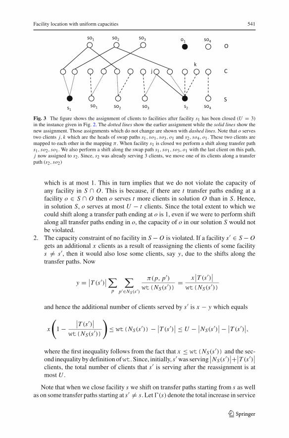
Fig. 3 The figure shows the assignment of clients to facilities after facility s1 has been closed (U = 3)in the instance given in Fig. 2. The dotted lines show the earlier assignment while the solid lines show thenew assignment. Those assignments which do not change are shown with dashed lines. Note that o servestwo clients j, k which are the heads of swap paths s1, so1, so3, o1 and s2, so4, o1. These two clients aremapped to each other in the mapping π . When facility s1 is closed we perform a shift along transfer paths1, so2, so1. We also perform a shift along the swap path s1, so1, so3, o1 with the last client on this path,j now assigned to s2. Since, s2 was already serving 3 clients, we move one of its clients along a transferpath (s2, so2)

which is at most 1. This in turn implies that we do not violate the capacity ofany facility in S ∩ O . This is because, if there are t transfer paths ending at afacility o ∈ S ∩ O then o serves t more clients in solution O than in S. Hence,in solution S, o serves at most U − t clients. Since the total extent to which wecould shift along a transfer path ending at o is 1, even if we were to perform shiftalong all transfer paths ending in o, the capacity of o in our solution S would notbe violated.

2. The capacity constraint of no facility in S− O is violated. If a facility s′ ∈ S− Ogets an additional x clients as a result of reassigning the clients of some facilitys �= s′, then it would also lose some clients, say y, due to the shifts along thetransfer paths. Now

y = ∣∣T (s′)

∣∣∑

p

∑

p′∈NS(s′)

π(p, p′)wt(NS(s′))

= x∣∣T (s′)

∣∣

wt(NS(s′))

and hence the additional number of clients served by s′ is x − y which equals

x

(

1−∣∣T (s′)

∣∣

wt(NS(s′))

)

≤ wt(NS(s′))− ∣∣T (s′)

∣∣ ≤ U − ∣

∣NS(s′)∣∣− ∣

∣T (s′)∣∣,

where the first inequality follows from the fact that x ≤ wt(NS(s′)) and the sec-ond inequality by definition ofwt. Since, initially, s′was serving

∣∣NS(s′)

∣∣+∣

∣T (s′)∣∣

clients, the total number of clients that s′ is serving after the reassignment is atmost U .

Note that when we close facility s we shift on transfer paths starting from s as wellas on some transfer paths starting at s′ �= s. Let �(s) denote the total increase in service

123


cost due to shifts on all transfer paths when facility s is closed. Consider a transferpath, q, starting from s. We would shift once along path q when we close facility s. Wewould also be shifting along q to an extent of

∑p∑

p′∈NS(s) π(p, p′)/wt(NS(s))(which is at most 1) when facilities other than s are closed. Hence,

∑

s

�(s) ≤ 2∑

q∈Tshift(q) (13)

For a swap path p, define res-wt(p) = 1 − wt(p). Let j be head(p) anddefine wt( j) = wt(p) and res-wt( j) = res-wt(p). Let p start from facilitys. When s is closed, client j is assigned to an extent wt( j) to other facilities in S.We will be assigning the remaining part of j to a facility o ∈ O − S that will beopened when s is closed. Hence the total number of clients that will be assigned too is res-wt(NS(s)) which is less than U . The increase in service cost due to thisreassignment is at most cs,ores-wt(NS(s)). As done earlier, the inequality corre-sponding to the swap 〈s, o〉 is counted to an extent λs,o in the linear combination.Since cs,o ≤ length(p) for all p ∈ N o

s , we have the following equivalent of Lemma 3

∑

s,o

λs,ocs,ores-wt(NS(s)) ≤∑

p∈Sres-wt(p)length(p). (14)

The remaining available capacity of o is utilized by assigning each client j ∈ NO(o)

to an extent βs,ores-wt( j), where βs,o is defined as before. This assignment is actu-ally done by shifting along each path, p ∈ NO(o), by an extent βs,ores-wt(p). LetΔ′(s, o) be the increase in cost due to this reassignment of clients in NO(o). Then

Δ′(s, o) ≤ βs,o

∑

p∈NO (o)

res-wt(p)shift(p).

This operation is a part of 〈s, o〉 and hence is counted to an extent λs,o in the linearcombination. Therefore the contribution of this term is

∑

s,o

λs,oΔ′(s, o) ≤

∑

o

(∑

s

λs,oβs,o

)∑

p∈NO (o)

res-wt(p)shift(p). (15)

Adding facility o ∈ O−S and shifting each path p ∈ NO(o) by an extentres-wt(p)gives us the following inequality.

fo +∑

p∈NO (o)

res-wt(p)shift(p) ≥ 0 (16)

As before, if∑

s λs,oβs,o > 1 then we reduce some βs,o so that the sum is exactly 1.Else, we add a 1−∑

s λs,oβs,o multiple of inequality (16) to inequality (15) to get

123


∑

s,o

λs,oΔ′(s, o) ≤

∑

o

γo fo +∑

o

∑

p∈NO (o)

res-wt(p)shift(p). (17)

where γo = max{0, 1−∑

s λs,oβs,o}.

The inequality corresponding to the swap 〈s, o〉 is

fo − fs + cs,ores-wt(NS(s))+Δ(s)+ �(s)+Δ′(s, o) ≥ 0,

and taking a linear combination of the inequalities corresponding to the swaps 〈s, o〉,s ∈ S − O , o ∈ O − S with weights λs,o yields

∑

s,o

λs,o fo −∑

s,o

λs,o fs +∑

s,o

λs,ocs,ores-wt(NS(s))

+∑

s,o

λs,o(Δ(s)+ �(s))+∑

s,o

λs,oΔ′(s, o) ≥ 0.

Since, for all s,∑

o λs,o = 1, we get

∑

s∈S−O

fs ≤∑

s,o

λs,o fo +∑

s,o

λs,oΔ′(s, o)

+∑

s,o

λs,ocs,ores-wt(NS(s))+∑

s

(Δ(s)+ �(s)) (18)

Putting the bounds from inequalities (12),(13),(14) and (17) into the right hand sideof inequality (18), yields

∑

s∈S−O

fs ≤∑

o∈O−S

(

γo +∑

s

λs,o

)

fo +∑

p∈Sres-wt(p)shift(p)

+∑

p∈Sres-wt(p)length(p)+

∑

p∈Swt(p)(shift(p)+ length(p))

+2∑

p∈Tshift(p)

≤ 2∑

o∈O−S

fo +∑

p∈Sres-wt(p)(shift(p)+ length(p))

+∑

p∈Swt(p)(shift(p)+ length(p))+ 2

∑

p∈Tshift(p)

= 2∑

o∈O−S

fo +∑

p∈S(shift(p)+ length(p))+ 2

∑

p∈Tshift(p)

≤ 2

⎛

⎝∑

o∈O−S

fo +∑

j∈C

O j

⎞

⎠

123


where the first inequality follows from Lemmas 5 and 4. This implies that

∑

s∈S

fs ≤ 2

⎛

⎝∑

o∈O−S

fo +∑

j∈C

O j

⎞

⎠+∑

o∈S∩O

fo ≤ 2

⎛

⎝∑

o∈O

fo +∑

j∈C

O j

⎞

⎠

which is the statement of Theorem 2 when S ∩ O �= φ.

5 A tight example

Our tight example consists of r facilities in the optimum solution O , r facilities inthe locally optimum solution S and rU clients. The facilities are F = O ∪ S. Sinceno facility can serve more than U clients, each facility in S and O serves exactly Uclients. Our instance has the property that a facility in O and a facility in S share atmost one client.

We can view our instance as a set-system—the set of facilities O is the ground setand for every facility s ∈ S we have a subset Xs of this ground set. o ∈ Xs iff thereis a client which is served by s in the solution S and by o in the solution O . Thisimmediately implies that each element of the ground set is in exactly U sets and thateach set is of size exactly U . A third property we require is that two sets have at mostone element in common.

We now show how to construct a set system with the properties mentioned above.With every o ∈ O we associate a distinct point xo = (xo

1 , xo2 , . . . xo

U ) in a U -dimen-sional space where for all i , xo

i ∈ {1, 2, 3, . . . , U }. For every choice of coordinate i ,1 ≤ i ≤ U we form UU−1 sets, each of which contains all points differing only incoordinate i . Thus the total number of sets we form is r = UU which is the same asthe number of points. Each set can be viewed as a line in U -dimensional space. Tosee that this set system satisfies all the properties note that each line contains U pointsand each point is on exactly U lines. It also follows from our construction that twodistinct lines meet in at most one point.

We now define the facility and the service costs. For a facility o ∈ O , fo = 2Uwhile for facility s ∈ S, fs = 6U − 6. For a client j ∈ N o

s , we have cs, j = 3 andco, j = 1. All other service costs are given by the metric property.

Lemma 6 For a client j and facility s ∈ S, the three smallest values that cs, j canhave are 3,5 and 11. Similarly, the three smallest values that co, j , o ∈ O can have are1,7 and 9.

Proof A client j can be served at a cost 1 by exactly one facility in O and at a cost 3by exactly one facility in S. The distance between a facility in O and a facility in S isat least 4. �

Since the service cost of each client in O is 1 and the facility cost of each facilityin O is 2U , we have cost(O) = 3UU+1. Similarly, cost(S) = (3− 2/U )3UU+1 andhence cost(S) = (3− 2/U )cost(O). We now need to prove that S is indeed a locallyoptimum solution with respect to the local search operations of add, delete and swap.

123


Adding a facility o ∈ O to the solution S, would incur an opening cost of 2U .The optimum assignment would reassign only the clients in No(O), and all these areassigned to o. The reduction in the service cost due to this is exactly 2U which is offsetby the increase in the facility cost. Hence the cost of the solution does not improve.

If we delete a facility in the solution S, the solution is no longer feasible since thetotal capacity of the facilities is now UU+1 −U and the number of clients is UU+1.

Now, consider swapping a facility s ∈ S with a facility o ∈ O . The net decreasein the facility cost is 4U − 6. To bound the increase in service costs we consider abipartite graph with the facilities S ∪ {o} and the clients C forming the two sides ofthe bipartition. Let E be the edges corresponding to the original assignment of clientsto facilities and E ′ be the edges of the new assignment. The symmetric differenceof E and E ′ is a collection of U edge-disjoint paths between s and o. Let P be thiscollection and P be one of these paths. We define the net-cost of P as the differencebetween the costs of the edges of E ′ and E in P .

Lemma 7 The two paths in P with the smallest net-cost have a total net-cost of atleast 2. All other paths in P have net-cost of at least 4.

Note that the increase in service cost as a result of the swap 〈s, o〉 equals the totalnet-cost of the paths in P . The lemma implies that the net-cost of the paths is at least4(U − 2)+ 2 which is exactly equal to the decrease in facility cost. Hence, swappingany pair of facilities s ∈ S and o ∈ O does not improve the solution.

Proof The edges of E on path P have cost 3. From Lemma 6 it follows that the edgeon path P incident to o has cost 1,7 or higher while the remaining edges of P ∩ E ′have cost 5,9 or higher. Edges on P alternate between sets E and E ′. Hence startingfrom s we can pair consecutive edges of P with the first edge of each pair from E andthe other from E ′. Note that every pair, except the last, contributes at least 2 to thenet-cost of P while the last pair contributes at least −2.

1. If the edge of P incident to o has cost 7 or higher then the last pair contributes atleast 4 to the net-cost of P and hence the net-cost of P is at least 4.

2. If any edge of P ∩ E ′ has cost 9 or higher then the corresponding pair contributesat least 6 to the net-cost. Since the last pair contributes at least−2, the net-cost ofP is at least 4.

As a consequence of the above we can assume that all edges of P ∩ E ′ have cost 5,except the edge incident to o which has cost 1. This implies that the path P correspondsto a path S1, S2, . . . Sk in our set-system where consecutive sets have a common ele-ment and S1 corresponds to facility s while Sk contains the element correspondingto o. Alternatively, in our construction of the set-system, the path P corresponds to asequence of lines where consecutive lines in the sequence intersect and the first line isthe one corresponding to facility s while the last line contains the point correspond-ing to o. Note that the paths in P are edge-disjoint but not vertex-disjoint. Hence thesequence of lines corresponding to two paths in P may have common lines but nopair of consecutive lines can be common in the two sequences. Further, the sequencesshould end in different lines.

A path P containing k sets, corresponds to a sequence of lines containing k linesand has a net-cost of 2(k − 2). Hence paths with 4 or more lines have a net-cost at

123


Fig. 4 U = 3. The figure shows the three cases corresponding to P0 having length 1, 2 and 3. P0 is thedotted path, P1 is the path with small dashes while P2 is the path with longer dashes

least 4 and so to prove the lemma we need to argue that there are at most 2 paths inP having less than 4 lines. Let P0, P1 be the two paths with the smallest lengths withP0 being the smallest.

1. If P0 has length 1 then the line corresponding to s, say ys , contains the point cor-responding to o, say xo. From our construction it follows that any other sequenceof lines which starts with ys and ends with a line containing xo which is differentfrom ys must contain at least 4 lines (including line ys). Hence path P1 has anet-cost at least 4. Thus the total net-cost of paths P0 and P1 is at least 2 (seeFig. 4).

2. If P0 has length 2 then the line ys and the point xo, have identical values forU − 2 coordinates. Let ya be the line in P0 containing xo. Once again, from ourconstruction it follows that any other sequence of lines which starts with ys andends with a line containing xo which is different from ya must contain at least3 lines. Hence P1 has length at least 3 and so the total net-cost of paths P0 andP1 is at least 2. Further the other paths of P would end with lines which are indimensions other than the last lines of P0, P1 and so the length of these paths isat least 4 (see Fig. 4).

3. If P0 has length 3 then ys and xo have identical values for U − 3 coordinates. Inthis case, the net-cost of paths P0, P1 is at least 2 and the other paths of P have atleast 4 lines (see Fig. 4).

�

6 Conclusions

While the local search algorithm for capacitated facility location is easy to specify,the analysis, even for the case of uniform capacities, can be quite involved. Ana-lyzing the more general case of non-uniform capacities would be quite a challenge.This suggests that one should explore other, non-LP, non-local-search approaches tocapacitated facility location.

References

1. Arya, V., Garg, N., Khandekar, R., Meyerson, A., Munagala, K., Pandit, V.: Local search heuristics fork-median and facility location problems. SIAM J. Comput. 33(3), 544–562 (2004)

123


2. Charikar, M., Guha, S.: Improved combinatorial algorithms for the facility location and k-median prob-lems. In: Proceedings of the 40th Annual IEEE Symposium on Foundations of Computer Science,pp. 378–388 (1999)

3. Chudak, F., Williamson, D.P.: Improved approximation algorithms for capacitated facility location prob-lems. Math. Program. 102(2), 207–222 (2005)

4. Korupolu, M.R., Plaxton, C.G., Rajaraman, R.: Analysis of a local search heuristic for facility locationproblems. J. Algorithms 37(1), 146–188 (2000)

5. Mahdian, M., Pál, M.: Universal facility location. In: Proceedings of the 11th Annual European Sym-posium on Algorithms, volume 2832 of Lecture Notes in Computer Science, pp. 409–421 (2003)

6. Mahdian, M., Ye, Y., Zhang, J.: A 2-approximation algorithm for the soft-capacitated facility loca-tion problem. In: Proceedings of the 6th International Workshop on Approximation Algorithms forCombinatorial Optimization, volume 2764 of Lecture Notes in Computer Science, pp. 129–140 (2003)

7. Pál, M., Tardos, É., Wexler, T.: Facility location with nonuniform hard capacities. In: FOCS ’01: Pro-ceedings of the 42nd IEEE symposium on Foundations of Computer Science, p. 329. IEEE ComputerSociety, Washington, DC, USA (2001)

8. Zhang, J., Chen, B., Ye, Y.: A multiexchange local search algorithm for the capacitated facility locationproblem. Math. Oper. Res. 30(2), 389–403 (2005)

123

a 3-approximation algorithm for the facility location problem with uniform capacities

Documents