Approximation Algorithms for Non-Uniform Buy-at-Bulk Network Design Problems

Mohammad R. SalavatipourDepartment of Computing Science

University of Alberta

Joint work with

C. Chekuri (Bell Labs)M.T. Hajiaghayi (CMU)G. Kortsarz (Rutgers)

2

Motivation

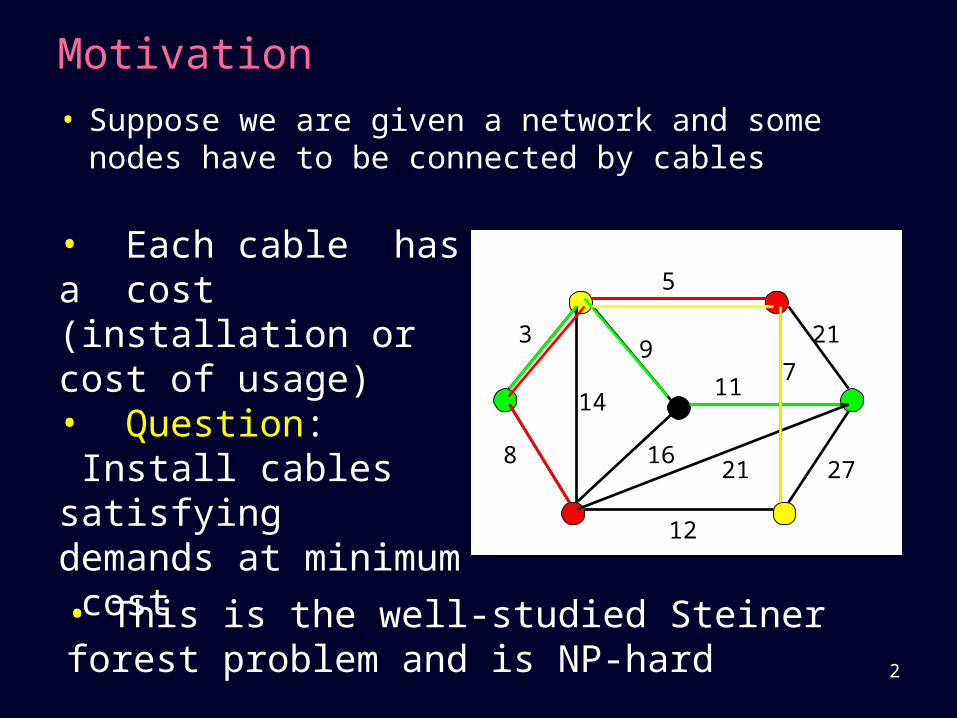
• Suppose we are given a network and some nodes have to be connected by cables

10

12

8

21

27

11

5

9

147

21

3

16

• Each cable has a cost (installation or cost of usage)• Question: Install cables satisfying demands at minimum cost

• This is the well-studied Steiner forest problem and is NP-hard

3

Motivation (cont’d)

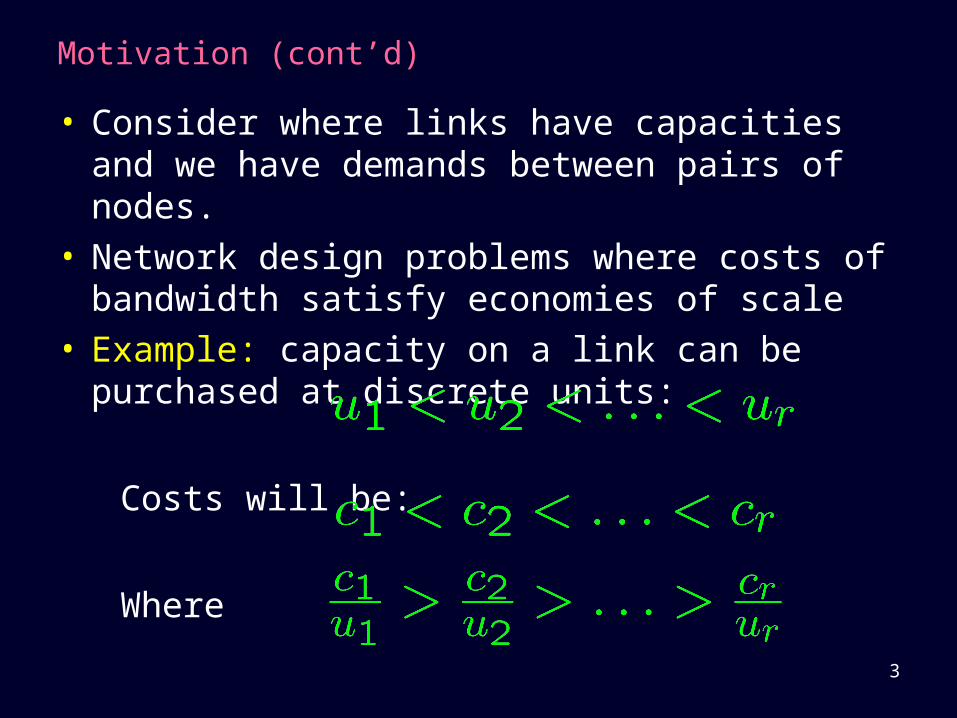
• Consider where links have capacities and we have demands between pairs of nodes.

• Network design problems where costs of bandwidth satisfy economies of scale

• Example: capacity on a link can be purchased at discrete units:

Costs will be:

Where

4

• So if you buy at bulk you save• More generally, we have a concave function

where f(b) is the minimum cost of cables with bandwidth b.

Motivation (cont’d)

bandwidth

cost

Question: Given a set of bandwidth demands between nodes, install sufficient capacities at minimum cost

5

Motivation (cont’d)

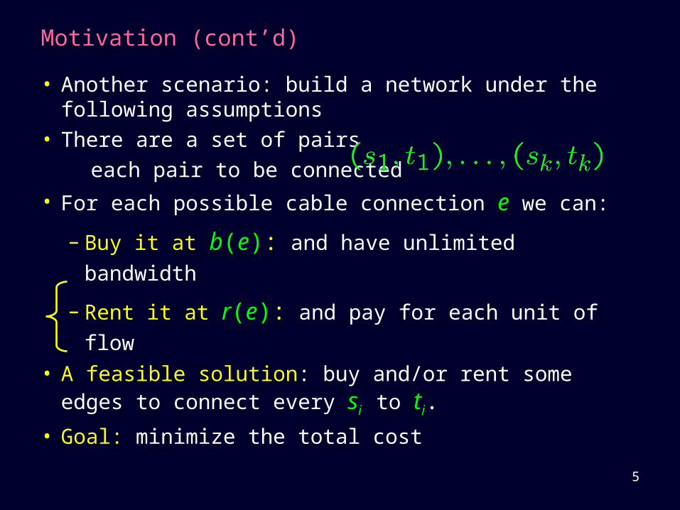
• Another scenario: build a network under the following assumptions

• There are a set of pairs

each pair to be connected

• For each possible cable connection e we can:

– Buy it at b(e): and have unlimited bandwidth

– Rent it at r(e): and pay for each unit of flow

• A feasible solution: buy and/or rent some edges to connect every si to ti.

• Goal: minimize the total cost

6

Motivation (cont’d)

10

14

3

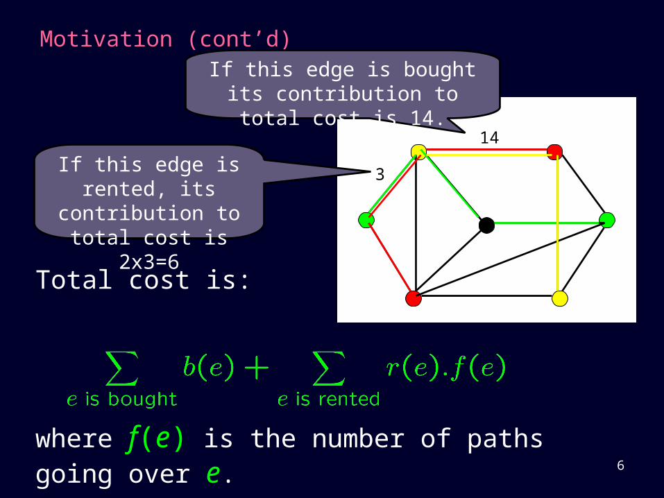
If this edge is bought its contribution to total cost is 14.

If this edge is rented, its contribution to total

cost is 2x3=6

Total cost is:

where f(e) is the number of paths going over e.

7

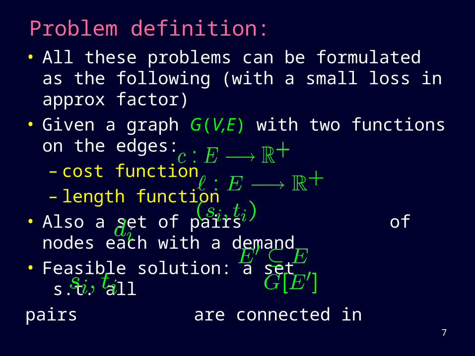
• All these problems can be formulated as the following (with a small loss in approx factor)

• Given a graph G(V,E) with two functions on the edges: – cost function– length function

• Also a set of pairs of nodes each with a demand

• Feasible solution: a set s.t. all

pairs are connected in

Problem definition:

8

Problem definition (cont’d)

• Note that the solution may have cycles

• This version of the problem is called

multi-commodity buy-at-bulk (MC-BB)

• Goal is to minimize the cost, where the cost is defined as follows

5

11

8

21

12

9

Problem definition (cont’d)

• The cost of the solution is:

where is the shortest path in • We can think of as the start-up cost and

as the per/use cost (length).

• Goal: minimize total cost.

10

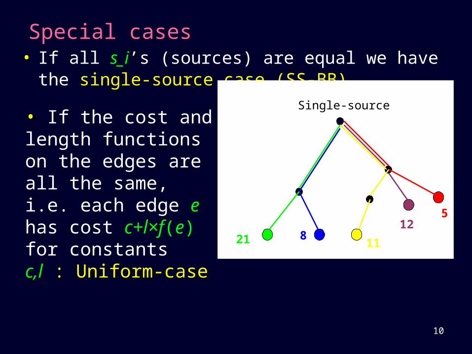
Special cases• If all s_i’s (sources) are equal we have the single-

source case (SS-BB)

• If the cost and length functions on the edges are all the same, i.e. each edge e has cost c+l×f(e) for constants c,l : Uniform-case

5

11821

12

Single-source

11

Some notation

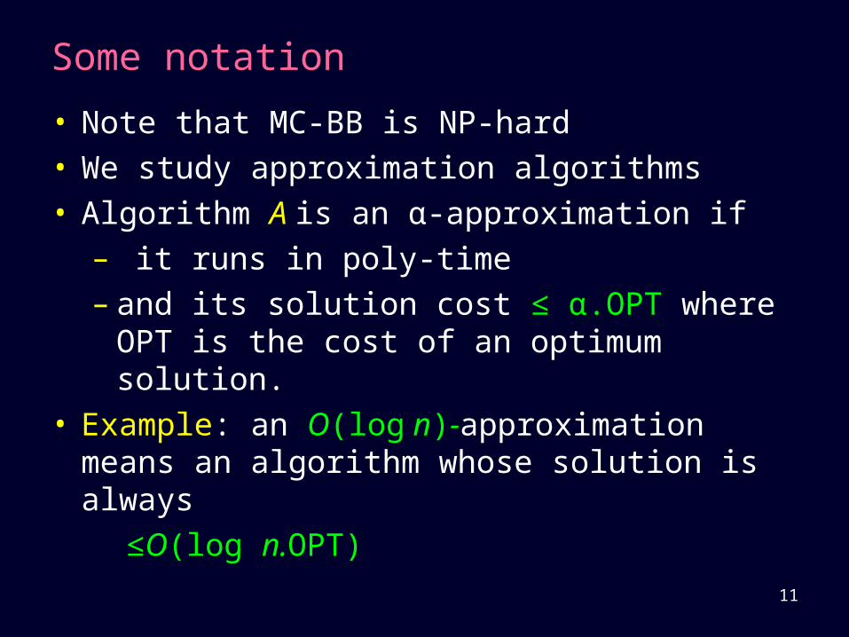
• Note that MC-BB is NP-hard • We study approximation algorithms• Algorithm A is an α-approximation if

– it runs in poly-time – and its solution cost ≤ α.OPT where OPT is the

cost of an optimum solution.• Example: an O(log n)-approximation means an

algorithm whose solution is always

≤O(log n.OPT)

12

Known results for buy-at-bulk problems• Formally introduced by [SCRS’97] • O(log n) approximation for the uniform case, i.e.

each edge e has cost c+l×f(e) for some fixed constants c, l [AA’97, Bartal’98]

• O(log n) approx for the single-sink case [MMP’00]• Hardness of ΩΩ(log log n) for the single-sink case

[CGNS’05] and ΩΩ(log1/2- n) in general [Andrews’04], unless NP ZPTIME(npolylog(n))

• Constant approx for several special cases: [AKR’91,GW’95,KM’00,KGR’02,KGPR’02,GKR’03]

• Best known factor for MC-BB [CK’05]:

13

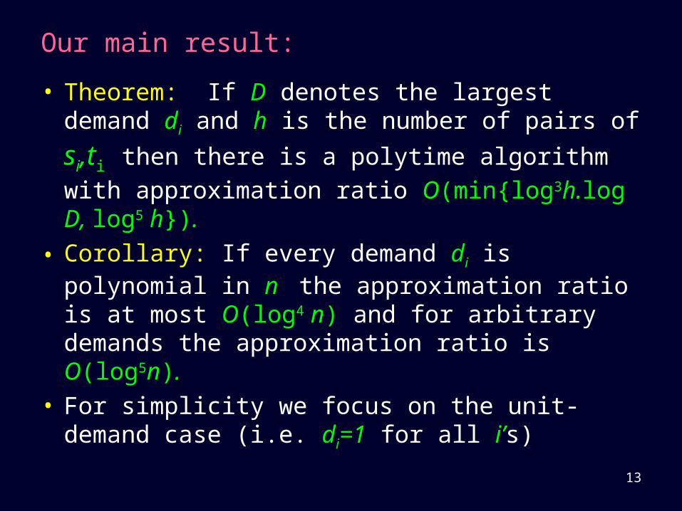
Our main result:

• Theorem: If D denotes the largest demand di

and h is the number of pairs of si,ti then there is

a polytime algorithm with approximation ratio O(min{log3h.log D, log5 h}).

• Corollary: If every demand di is polynomial in n the approximation ratio is at most O(log4 n) and for arbitrary demands the approximation ratio is O(log5n).

• For simplicity we focus on the unit-demand case (i.e. di=1 for all i’s)

14

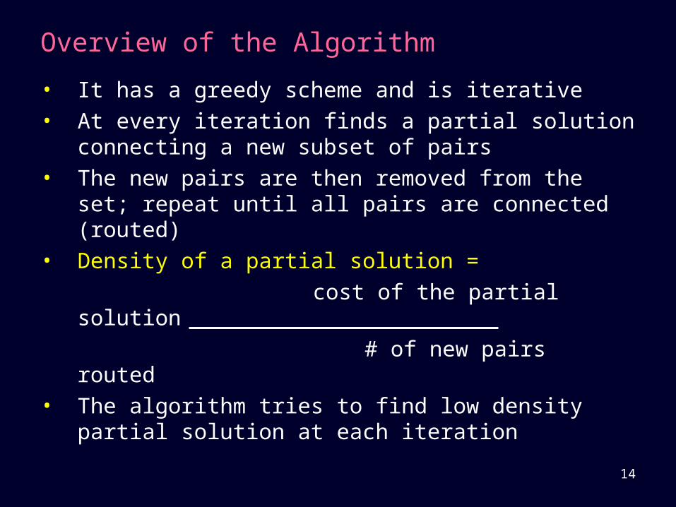
Overview of the Algorithm

• It has a greedy scheme and is iterative• At every iteration finds a partial solution

connecting a new subset of pairs• The new pairs are then removed from the set;

repeat until all pairs are connected (routed)• Density of a partial solution =

cost of the partial solution

# of new pairs routed• The algorithm tries to find low density partial

solution at each iteration

15

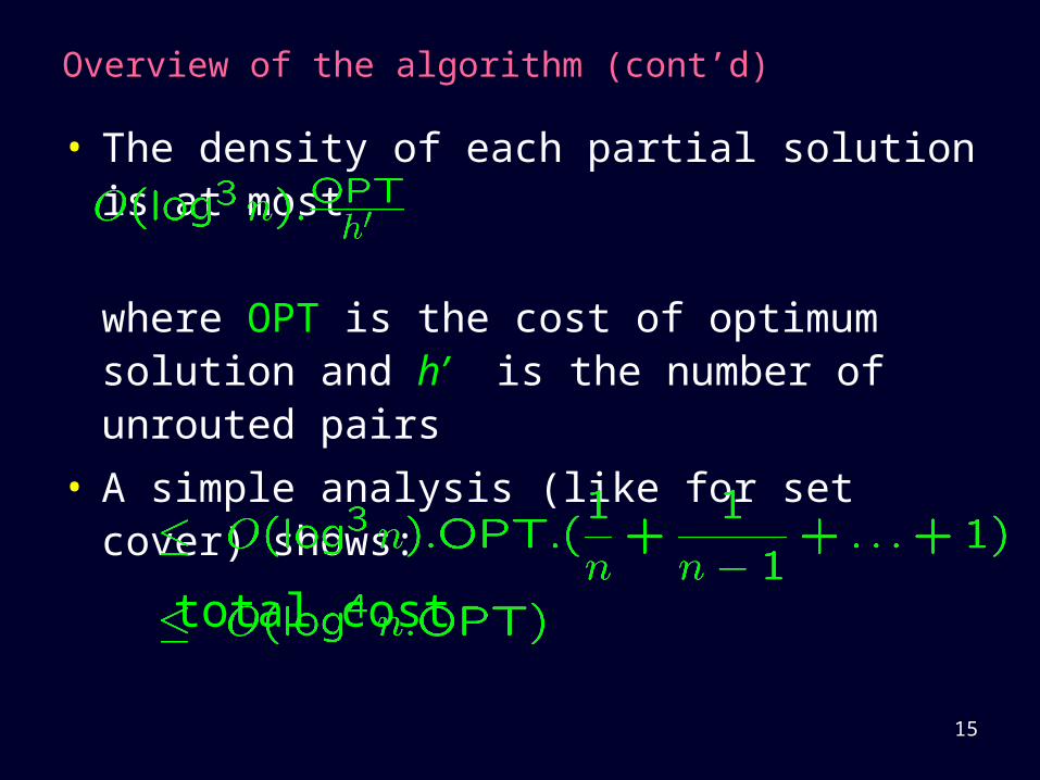
Overview of the algorithm (cont’d)

• The density of each partial solution is at most

where OPT is the cost of optimum solution and h’ is the number of unrouted pairs

• A simple analysis (like for set cover) shows:

total cost

16

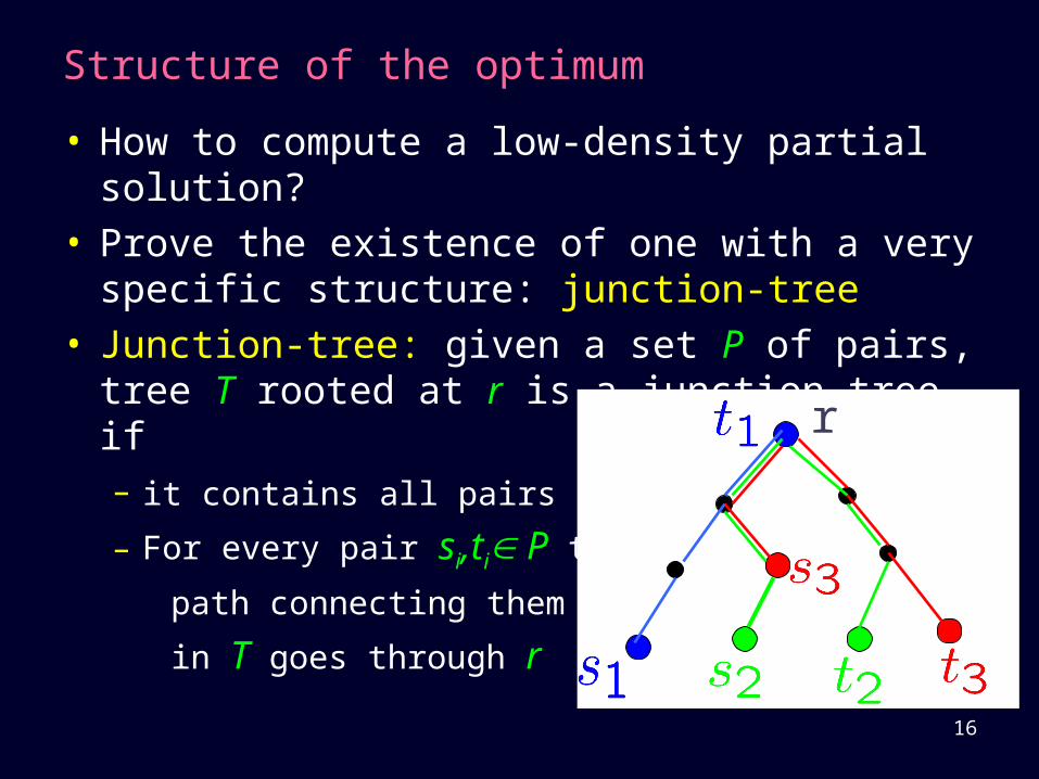
Structure of the optimum

• How to compute a low-density partial solution?• Prove the existence of one with a very specific

structure: junction-tree• Junction-tree: given a set P of pairs, tree T

rooted at r is a junction tree if – it contains all pairs of P

– For every pair si,ti P the

path connecting them

in T goes through r

r

17

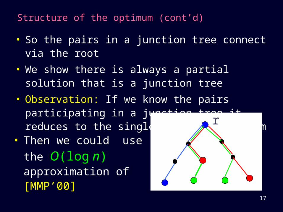
Structure of the optimum (cont’d)

• So the pairs in a junction tree connect via the root

• We show there is always a partial solution that is a junction tree

• Observation: If we know the pairs participating in a junction-tree it reduces to the single-source BB problem r

• Then we could use the

O(log n) approximation of [MMP’00]

18

Summary of the algorithm

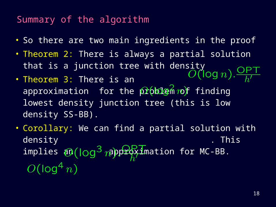
• So there are two main ingredients in the proof

• Theorem 2: There is always a partial solution that is a junction tree with density

• Theorem 3: There is an approximation for the problem of finding lowest density junction tree (this is low density SS-BB).

• Corollary: We can find a partial solution with density . This implies an

approximation for MC-BB.

19

More details of the proof of Theorem 2:

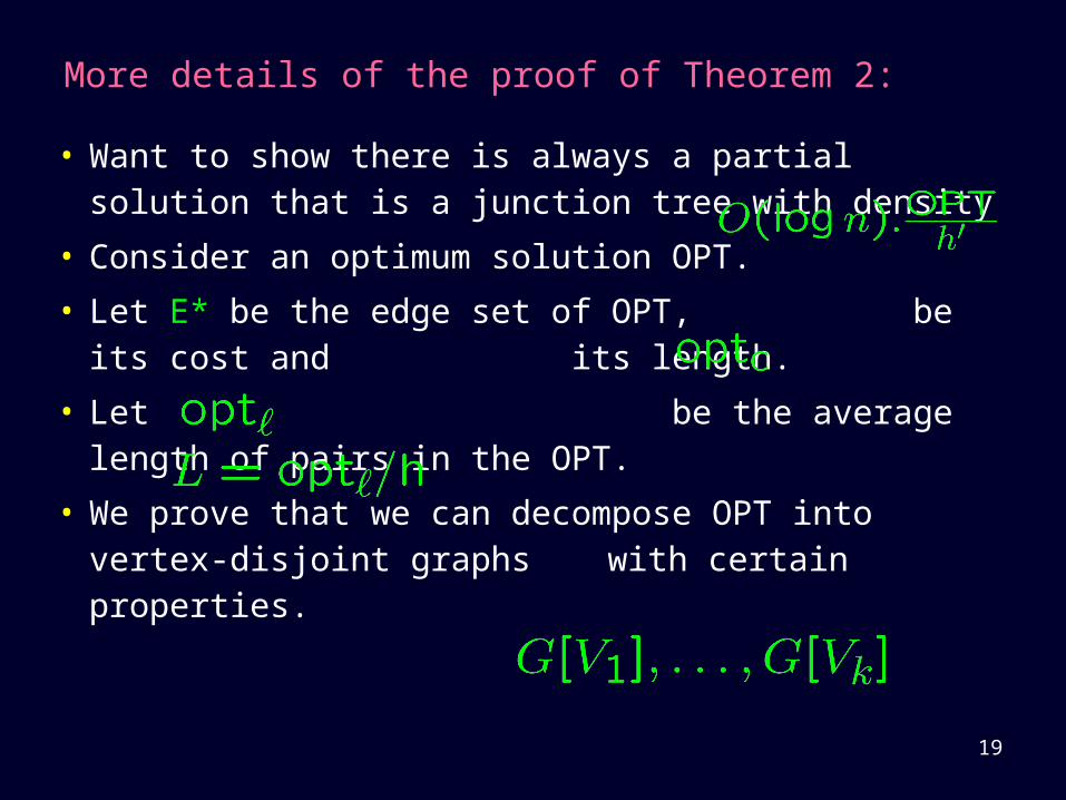
• Want to show there is always a partial solution that is a junction tree with density

• Consider an optimum solution OPT.

• Let E* be the edge set of OPT, be its cost and its length.

• Let be the average length of pairs in the OPT.

• We prove that we can decompose OPT into vertex-disjoint graphs with certain properties.

20

More details of the proof of Theorem 2:

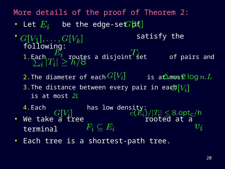
• Let be the edge-set of

• satisfy the following:

1. Each routes a disjoint set of pairs and

2. The diameter of each is at most

3. The distance between every pair in each is at most 2L

4. Each has low density:

• We take a tree rooted at a terminal

• Each tree is a shortest-path tree.

21

More details of the proof of Theorem 2:

• By diameter bound, distance of every node to in is at most

• The total cost of these trees is at most:

22

More details of the proof of Theorem 2:

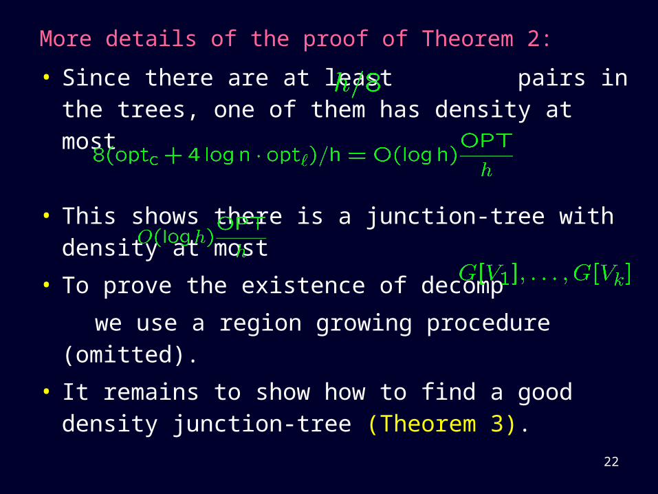
• Since there are at least pairs in the trees, one of them has density at most

• This shows there is a junction-tree with density at most

• To prove the existence of decomp

we use a region growing procedure (omitted).

• It remains to show how to find a good density junction-tree (Theorem 3).

23

Some details of the proof of Theorem 3:

• Theorem 3: There is an approximation for finding lowest density junction tree.

• This is very similar to SS-BB except that we have to find a lowest density solution.

• Here we have to connect a subset of terminals of a set to the source s with lowest density (= cost of solution / # of terminals in sol).

• Let denote the set of paths from s to ti.

• We formulate the problem as an IP and then consider the LP relaxation of the problem

24

Some details of the proof of Theorem 3:

• We solve the LP, and then based on the solution find a subset of nodes to solve the SS-BB on.

• We use the approx of [MMP,CKN] for SS-BB

• We loose another factor in the process of reduction to SS-BB (details omitted)

25

Some Remarks:

• For the polynomially bounded demand case we can find low density junction-trees using a greedy algorithm [HKS’06].

• This is the algorithm developed for a bicriteria version of the problem.

• For arbitrary demands, we use the upper bound of [DGR’05,EEST’05] (which is ) for distortion in embedding a finite metric into a probability distribution over its spanning tree.

26

Some Remarks (cont’d):

• This is why we get a factor of for approximation factor comparing to

for polynomially bounded demands.

• There is a conjectured upper bound of

for distortion in embedding a metric into a probability distribution over its spanning tree.

• If true, that would improve our approximation factor for arbitrary demands to

27

Discussion and open problems

• The results can be extended to the vertex-weighted case but requires some new ideas and some extra work [CHKS’06].

• There are still quite large gaps between upper bounds (approx alg) and lower bounds (hardness)

– For MC-BB: vs

– For SS-BB: vs

• It would be nice to upper bound the integrality gap for MC-BB.