7 multivariate time series, linear systems and...

7

MULTIVARIATE TIME SERIES,LINEAR SYSTEMS AND

KALMAN FILTERING

This chapter is devoted to the analysis of the time evolution of random vectors. Thefirst section presents the generalization to the multivariate case of the univariate timeseries models studied in the previous chapter. Modern accounts of time series anal-ysis increasingly rely on the formalism and the techniques developed for the analy-sis of general stochastic systems. Even though financial applications have remainedmostly immune to this evolution, because of its increased popularity and its tremen-dous potential, we decided to include this alternative approach in this chapter. Thetone of the chapter will have to change slightly as we discuss concepts and theorieswhich were introduced and developed in engineering fields far remote from financialapplications. The practical algorithms were developed mostly for military applica-tions. They led to many civil and technological breakthroughs. Here, we present themain features of the filtering algorithms, and we use financial examples as illustra-tions, restricting ourselves to linear systems.

7.1 MULTIVARIATE TIME SERIES

Multivariate time series need to be introduced and used when significant dependen-cies between individual time series cannot be ignored. As an illustration, we discussfurther the weather derivative market, and some of the natural issues faced by itsparticipants. An active market maker in these markets will want to hold options writ-ten on HDD’s and/or CDD’s in different locations. One good reason for that maybe the hope of taking advantage of the possible correlations between the weather(and hence the temperature) in different locations. Also large businesses with sev-eral units spread out geographically are likely to want deals structured to fit theirdiverse weather exposures, and this usually involves dealing with several locationssimultaneously. Think for example of a chain of amusement parks, or a large retailersuch as Wal-Mart or Home Depot: their weather exposures are tied to the geographiclocations of the business units, and an analysis of the aggregate weather exposurecannot be done accurately by considering the locations separately and ignoring thecorrelations. As we are about to show, the simultaneous tracking of the weather in

AZhao

Highlight

AZhao

Highlight

378 7 MULTIVARIATE TIME SERIES, LINEAR SYSTEMS & KALMAN FILTERING

several locations can be best achieved by considering multivariate time series. Wediscuss a specific example in Subsection 7.1.4 below.

The goal of this section is to review the theory of the most common models ofmultivariate time series, and to emphasize the practical steps to take in order to fitthese models to real data. Most of the Box-Jenkins theory of the ARIMA modelspresented earlier can be extended to the multivariate setting. However, as we shallsee, the practical tools become quite intricate when we venture beyond the auto-regressive models. Indeed, even though the definition of moving average processescan be generalized without change, fitting this class of models becomes even morecumbersome than in the univariate case. As a side remark we mention that R doesnot provide any tool to fit multivariate moving average models.

In terms of notation, we keep using the convention followed so far in the book:as a general rule, we use bold face characters for multivariate quantities (i.e. vectorsfor which d > 1) and regular fonts for univariate quantities (i.e scalars for whichd = 1). In particular, throughout the rest of this section, we shall use the notationX = Xtt to denote a multivariate time series. In other words, for each time stampt, Xt is a d-dimensional random vector.

7.1.1 Stationarity and Auto-Covariance Functions

Most of what was said concerning stationarity extends without any change to themultivariate case. This includes the definition and the properties of the shift operatorB, and the derivative (time differentiation) operator ∇. Remember that stationarityis crucial for the justification of the estimation of the statistics of the series by timeaverages. The structure of the auto-covariance/correlation function is slightly differ-ent in the case of multivariate time series. Indeed, for each value k of the time lag,the lag-k auto-covariance is given by a matrix γ(k) = [γij(k)]i,j defined by:

γij(k) = EX(i)t X

(j)t+k − EX(i)

t EX(j)t+k.

In other words, the quantity γij(k) gives the lag-k cross-correlation between the i-thand j-th components of X, i.e. the covariance of the scalar random variables X(i)

t

and X(j)t+k.

7.1.2 Multivariate White Noise

As in the case of univariate series, the white noise series are the building blocks ofthe time series edifice. A multivariate stationary time series W = Wtt is said tobe a white noise if it is:

• mean-zero (i.e. EWt = 0 for all t);• serially uncorrelated

– either in the strong sense, i.e. if all the Wt’s are independent of each other;– or in the weak sense, i.e. if EWtW

ts = 0 whenever s 6= t.

AZhao

Highlight

7.1 Multivariate Time Series 379

The equality specifying the fact that a white noise needs to be mean zero is anequality between vectors. If d is the dimension of the vectors Wt, then this equal-ity is equivalent to a set of d equalities between numbers, i.e. EW (i)

t = 0 fori = 1, . . . , d. As usual, we use the notation W (i)

t for the i-th component of the vec-tor Wt. On the other hand, the last equality is an equality between d×dmatrices, andwhenever s 6= t, it has to be understood as a set of d×d equalities EW (i)

t W(j)s = 0

for i, j = 1, . . . , d.This is exactly the same definition as in the scalar case in the sense that there iscomplete de-correlation in the time variable. But since the noise terms are vectors,there is also the possibility of correlation between the various components. In otherwords,

at each time t, the components of Wt can be ”correlated”.

Hence, in the case of a white noise, we have

γi,j(k) = EW (i)t W

(j)t+k = γi,jδ0(k)

where δ0(k) is the usual delta function which equals 1 when k = 0 and 0 whenk 6= 0, and γ = [γi,j ]i,j=1,...,k is a time independent variance/covariance matrix fora d-dimensional random vector. Using the jargon of electrical engineers we wouldsay that the components are white in time and possibly colored in space.

7.1.3 Multivariate AR Models

A d-dimensional time series X = Xtt is said to be an auto-regressive series oforder p if there exist d × d matrices A1, A2, . . . , Ap and a d-variate white noiseWtt such that:

Xt = A1Xt−1 +A2Xt−2 + · · ·+ApXt−p +Wt. (7.1)

As before we ignored the mean term (which would be a d-dimensional vector in thepresent situation) by assuming that all the components have already been centeredaround their respective means. Notice that the number of parameters is now pd2 +d(d + 1)/2 since we need d2 parameters for each of the p matrices A and we needd(d + 1)/2 parameters for the variance/covariance matrix ΣW of the white noise(remember that this matrix is symmetric so that we need only d(d+1)/2 coefficientsinstead of d2!). Except for the fact that the product of matrices is not commutative,AR models can be fitted in the same way as they are fitted in the univariate case,for example by solving the system of Yule-Walker linear equations obtained fromthe empirical estimates of the auto-covariance function and the consistency relationswith the definition (7.1). In fact as we are about to see, fitting auto-regressive modelswith the R function ar can be done with multivariate time series in exactly the sameway it is done with univariate series.

AZhao

Highlight

AZhao

Highlight


Fitting Multivariate AR Models in R

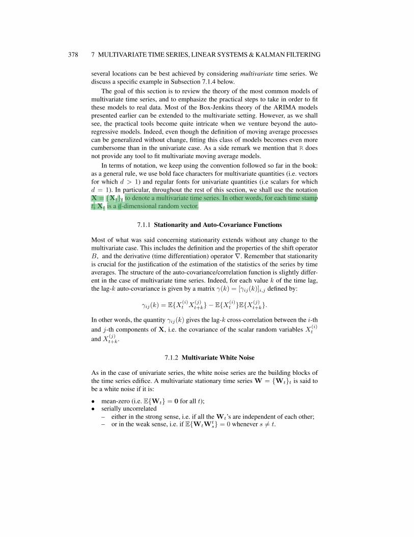
Before fitting a multivariate AR model we plot the auto-correlation function with thesame command acf as in the univariate case. In order to give an illustration, weuse the example of multivariate timeSeries object TEMPS . We shall create thistri-variate time series in Subsection 7.1.4 below.

> acf(TEMPS.ts)

The acf plot is reproduced in Figure 7.1. The output is a 3× 3 matrix of 9 plots (the

0 5 10 20 30

0.00.4

0.8

Lag

ACF

CVG

0 5 10 20 30

0.00.4

0.8

Lag

CVG & DM

0 5 10 20 30

0.00.4

0.8

Lag

CVG & PDX

-35 -25 -15 -5 0

0.00.4

0.8

Lag

ACF

DM & CVG

0 5 10 20 30

0.00.4

0.8

Lag

DM

0 5 10 20 300.0

0.40.8

Lag

DM & PDX

-35 -25 -15 -5 0

0.00.4

0.8

Lag

ACF

PDX & CVG

-35 -25 -15 -5 0

0.00.4

0.8

Lag

PDX & DM

0 5 10 20 30

0.00.4

0.8

Lag

PDX

Fig. 7.1. Auto-correlation functions of the 3-variate time series of original temperature data.

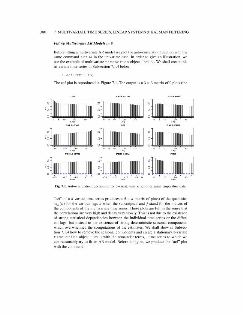
”acf” of a d-variate time series produces a d × d matrix of plots) of the quantitiesγi,j(k) for the various lags k when the subscripts i and j stand for the indices ofthe components of the multivariate time series. These plots are full in the sense thatthe correlations are very high and decay very slowly. This is not due to the existenceof strong statistical dependencies between the individual time series or the differ-ent lags, but instead to the existence of strong deterministic seasonal componentswhich overwhelmed the computations of the estimates. We shall show in Subsec-tion 7.1.4 how to remove the seasonal components and create a stationary 3-variatetimeSeries object TEMPS with the remainder terms, , time series to which wecan reasonably try to fit an AR model. Before doing so, we produce the ”acf” plotwith the command:


> acf(TEMPS)

The result is given in Figure ??.

0 5 10 20 30

0.00.4

0.8

Lag

ACF

CVG_rem

0 5 10 20 30

0.00.4

0.8

Lag

CVG_ & DM_r

0 5 10 20 30

0.00.4

0.8

Lag

CVG_ & PDX_

-35 -25 -15 -5 0

0.00.4

0.8

Lag

ACF

DM_r & CVG_

0 5 10 20 30

0.00.4

0.8

Lag

DM_rem

0 5 10 20 30

0.00.4

0.8

Lag

DM_r & PDX_

-35 -25 -15 -5 0

0.00.4

0.8

Lag

ACF

PDX_ & CVG_

-35 -25 -15 -5 0

0.00.4

0.8

Lag

PDX_ & DM_r

0 5 10 20 30

0.00.4

0.8Lag

PDX_rem

Fig. 7.2. Auto-correlation functions of the 3-variate time series of temperature remainders.

We can now fit an AR model with the command:

> TEMPS.ar <- ar(TEMPS)

The order chosen by the fitting algorithm can be printed in the same way. The orderchosen for the three city temperature remainders analyzed below is 5. The orderwas chosen because of the properties of the AIC, but as in the univariate case, thecomputation of the partial auto-correlation functions should be used to check that thechoice of the order is reasonable.

> TEMPS.ar$order[1] 5> pacf(TEMPS)

The partial auto-correlation function can be obtained with the R function pacf orwith the generic function acf provided we add the parameter type to "partial"as in acf(TEMPS,type="partial"). Figure 7.3 shows that this value is indeedreasonable.


0 5 10 15 20 25 30 35

-0.2

0.20.6

Lag

Partia

l ACF

CVG_rem

0 5 10 15 20 25 30 35

-0.2

0.20.6

Lag

CVG_ & DM_r

0 5 10 15 20 25 30 35

-0.2

0.20.6

Lag

CVG_ & PDX_

-35 -25 -15 -5 0

-0.2

0.20.6

Lag

Partia

l ACF

DM_r & CVG_

0 5 10 15 20 25 30 35-0.2

0.20.6

Lag

DM_rem

0 5 10 15 20 25 30 35

-0.2

0.20.6

Lag

DM_r & PDX_

-35 -25 -15 -5 0

-0.2

0.20.6

Lag

Partia

l ACF

PDX_ & CVG_

-35 -25 -15 -5 0

-0.2

0.20.6

Lag

PDX_ & DM_r

0 5 10 15 20 25 30 35

-0.2

0.20.6

Lag

PDX_rem

Fig. 7.3. Partial auto-correlation functions of the 3-variate time series of temperature remain-ders.

Prediction

Except for the technical complexity of the computations which now involve matri-ces instead of plain numbers, our discussion of the univariate case applies to themultivariate case considered in this section.

For example, if A1, A2, . . . , Ap and ΣW are the estimates of a d-dimensionalAR(p) model (i.e. the parameters of a model fitted to a d-variate data set), then atany instant t (by which we mean at the end of the t-th time interval, when we knowthe exact values of the outcome Xs for s ≤ t), the prediction of the next value of theseries is given by:

Xt+1 = A1Xt + A2Xt−1 + · · ·+ ApXt−p+1. (7.2)

One can similarly derive the prediction of the value of the series two steps ahead, orfor any finite number of time steps in the future.

Xt+k = A1Xt+k−1 + A2Xt+k−2 + · · ·+ ApXt+k−p (7.3)

where we ought to replace the prediction Xs by the observed value Xs wheneveravailable, i.e. when s ≤ t. As in the univariate case, when the time series is stable, thelonger the horizon of the prediction, the closer it will be to the long term average ofthe series. We shall illustrate this fact on the numerical example we consider below.

For implementation purposes, the R generic function predict can be used inthe multivariate case as well. The only difference is that for multivariate predictions,


the generic function predict does not compute estimates of the prediction errors,returning NAs for these error estimates.

Monte Carlo Simulations & Scenarios Generation

As in the univariate case, random simulation should not be confused with prediction.For the sake of the present discussion, let us assume that we have the values of thevectors Xt, Xt−1, . . ., Xt−p+1 at hand, and that we would like to generate a specificnumber, say N , of Monte Carlo scenarios for the values of Xt+1, Xt+2, . . ., Xt+M .

The correct procedure is to generate N samples of a d-dimensional white noisetime series of length M , say Wss=t+1,...,t+M , with the variance/covariance ma-trix ΣW , and then to use the parameter estimates A1, A2, . . ., Ap and the recursiveformula (7.1) giving the definition of the AR(p) model to generate samples of the ARmodel from these N samples of the white noise. In other words, for each of the Ngiven samples W(j)

t+1, . . . , W(j)t+M of the white noise, we generate the corresponding

Monte Carlo scenarios of the series by computing recursively the values X(j)t+1, . . . ,

X(j)t+M from the formula:

X(j)t+k = A1X

(j)t+k−1+A2X

(j)t+k−2+· · ·+ApX

(j)t+k−p+W

(j)t+k, k = 1, 2, . . . ,M

(7.4)for j = 1, 2, . . . , N , given the fact that, like in the prediction case, the ”hats” overthe X’s (i.e. the simulations) are not needed when the true values are available.

7.1.4 Back to Temperature Options

We come back to temperature data and temperature options to give a concrete exam-ple of the practical use of multivariate time series fitting.

Hedging Several Weather Exposures

Let us assume for the sake of illustration, that most of the summer revenues of a com-pany selling thirst quenchers come from sales in Des Moines, Portland and Cincin-nati. Clearly, an unusually cool summer in these cities would hurt the company’srevenues, so the chief risk officer decided to approach a financial institution lookingfor a solution to mitigate the possible losses linked to such a weather exposure. Onecan imagine that this financial institution offers to sell the three call options whosecharacteristics are given in Table 7.1.4.

AZhao

Highlight

AZhao

Highlight

AZhao

Highlight


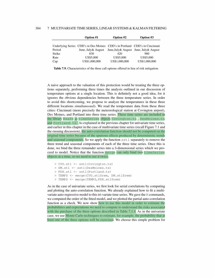
Option #1 Option #2 Option #3

Underlying Series CDD’s in Des Moines CDD’s in Portland CDD’s in CincinnatiPeriod June, July& August June,July& August June, July& AugustStrike 830 420 980Rate US$5,000 US$5,000 US$5,000Cap US$1,000,000 US$1,000,000 US$1,000,000

Table 7.9. Characteristics of the three call options offered in lieu of risk mitigation.

A naive approach to the valuation of this protection would be treating the three op-tions separately, performing three times the analysis outlined in our discussion oftemperature options at a single location. This is definitely not a good idea, for itignores the obvious dependencies between the three temperature series. In orderto avoid this shortcoming, we propose to analyze the temperatures in these threedifferent locations simultaneously. We read the temperature data from these threecities: Cincinnati (more precisely the meteorological station at Covington airport),Des Moines, and Portland into three time series. These time series are included inthe library Rsafd as timeSeries objects Covington.ts , DesMoines.tsand Portland.ts. As explained in the previous chapter for univariate time series,and earlier in this chapter in the case of multivariate time series (recall Figure 7.1 andthe ensuing discussion), the auto-correlation function should not be computed on theoriginal time series because of the spurious effects produced by deterministic trendsand seasonal components. So we apply the function sstl separately to remove thethree trend and seasonal components of each of the three time series. Once this isdone, we bind the three remainder series into a 3-dimensional series which we pro-ceed to model. Notice that the function merge can only bind two timeSeriesobjects at a time, so we need to use it twice.

> CVG.stl <- sstl(Covington.ts)> DM.stl <- sstl(DesMoines.ts)> PDX.stl <- sstl(Portland.ts)> TEMPS <- merge(CVG.stl$rem, DM.stl$rem)> TEMPS <- merge(TEMPS,PDX.stl$rem)

As in the case of univariate series, we first look for serial correlations by computingand plotting the auto-correlation function. We already explained how to fit a multi-variate auto-regressive model to this tri-variate time series. We gave the R commands,we computed the order of the fitted model, and we plotted the partial auto-correlationfunction as a check. We now show how to use this model in order to estimate theprobabilities and expectations we need to compute to understand the risks associatedwith the purchase of the three options described in Table 7.1.4. As in the univariatecase, we use Monte Carlo techniques to estimate, for example, the probability that atleast one of the three options will be exercised. We choose this simple problem for

AZhao

Highlight

AZhao

Highlight

AZhao

Highlight

AZhao

Highlight

AZhao

Highlight


the sake of illustration. Indeed, this probability is not of much practical interest. Itwould be more interesting to associate a cost/penalty/utility to each possible temper-ature scenario, and to compute the expected utility over all the possible scenarios. Inany case, this probability can be computed in the following way:

• Choose a large number of scenarios, say N = 10, 000;• Use the fitted model to generate N samples x(j)

t , x(j)t+1, . . ., x(j)

T where t corre-sponds to March 31st, 1999, and T to August 31st, 1999, j = 1, 2, . . . , N , andeach x

(j)t+s is a three dimensional vector representing the temperature remainders

in the three cities, on day t + s for the j-th scenario. Remember that accordingto the explanations given above, this is done by generating the white noise first,and then computing the x

(j)t+s inductively from formula (7.4).

• Add the mean temperatures and the seasonal components to each of the threecomponents to obtainN scenarios of the temperatures in Covington, Des Moines,and Portland starting from March 31st, 1999, and ending August 31st, 1999;

• For each single one of these N tri-variate scenarios, compute the number ofCDD’s between June 1st and August 31st in each of the three cities;

• Compute the number of times at least one of the three total numbers of CDD’s isgreater that the corresponding strike, and divide by N .

The Case of a Basket Option

Instead of purchasing three separate options, similar risk mitigation can be achievedby the purchase of a single option written on an index involving the temperatures inthe three locations. The simplest instruments available over the counter are writtenon an underlying index obtained by computing the plain average, or the sum, of theindexes used above for the three cities. In other words, we would compute the totalnumber of CDD’s in Des Moines over the summer, the total number of CDD’s inPortland over the same period, and finally the total number of CDD’s in Cincinnatiin the same way, add these three numbers, and compare this aggregate index to thestrike of the option. In other words, instead of being the sum of the three separate pay-offs, the pay-off of the option is a single function of an aggregate underlying index.Such options are called basket options. Obviously, the averages could be weighted

averages instead of plain averages, the analysis would be the same. Modeling the sep-arate underlying indexes simultaneously is a must in dealing with basket options. Itwould be unreasonable, borderline suicidal, not to include the dependencies betweenthese indexes in the model. Fortunately, the Monte Carlo analysis presented abovecan be performed in exactly the same way. For each of the N tri-variate scenariosgenerated above, one compute the numbers of CDD’s in each of the three locations,and add them up together: this is the underlying index. It is then plain to decide if theoption is exercised, or to compute the loss/utility associated to such a scenario forthe three locations, . . . and to compute probabilities of events of interest or desiredexpectations, by averaging over the scenarios.

AZhao

Highlight

AZhao

Highlight

AZhao

Highlight

AZhao

Highlight

AZhao

Highlight

AZhao

Highlight

AZhao

Highlight


7.1.5 Multivariate MA & ARIMA Models

This subsection is included for the sake of completeness only. None of the conceptsand results presented in this subsection will be used in the sequel (including theproblems).

A d-dimensional time series X = Xtt is said to be a moving average seriesof order q if there exist d × d matrices B1, B2, . . . , Bq and a d-variate white noiseWtt such that:

Xt = Wt +B1Wt−1 +B2Wt−2 + · · ·+BqWt−q

for all times t. As before we ignored the mean term (which would be a d-dimensionalvector in the present situation) by assuming that all the components have alreadybeen centered around their respective means. As in the case of a multivariate ARmodel, the number of parameters can be computed easily. This number of parametersis now qd2 + d(d + 1)/2. As in the univariate case, fitting moving average modelsis more difficult than for auto-regressive processes. It can be done by maximumlikelihood, but the computations require sophisticated recursive procedures and theyare extremely involved. This is the reason why R does not provide a function (similarto ar) to fit multivariate moving average time series.

A d-dimensional time series X = Xtt is said to be an ARMA(p,q) time seriesif there exist d× d matrices A1, A2, . . . , Ap, B1, B2, . . . , Bq , and a d-variate whitenoise Wtt such that:

Xt −A1Xt−1 −A2Xt−2 − · · · −ApXt−p = Wt +B1Wt−1 + · · ·+BqWt−q

Finally, as in the univariate case, an ARIMA(p,r,q) time series is defined as a timeseries which becomes an ARMA(p,q) after r differentiations.

Prediction and Simulation in R

Contrary to the univariate case, R does not provide any function to produce randomsamples of multivariate ARIMA time series. It does not have a function to computepredictions of future values from a general multivariate ARIMA model either. How-ever, the generic function predict can still be used with objects of class ar evenwhen the latter are multivariate.

7.1.6 Cointegration

The concept of cointegration is of crucial importance in the analysis of financialtime series. We define it in the simplest possible context: two I(1) time series. Seethe Notes & Complements at the end of the chapter for details and references.

Two unit-root time series are said to be cointegrated if there exists a linear combi-nation of its entries which is stationary. The coefficients of such a linear combinationare said to form a cointegration vector. For example, it has been argued that yields ofdifferent maturities are cointegrated.


Example

We first discuss an academic example for the purpose of illustration. Let us considertwo time series X(1)

n n=1,...,N and X(2)n n=1,...,N defined by:

X(1)n = Sn + ε(1)n and X(2)

n = Sn + ε(2)n , n = 1, . . . , N

where Sn = S0 + W1 + · · · + Wn is a random walk starting from S0 = 0 con-structed form the N(0, 1) white noise Wnn=1,...,N , and where ε(1)n n=1,...,N andε(2)n n=1,...,N are two independent N(0, .16) white noise sequences which are as-sumed to be independent of Wnn=1,...,N . Since the time series X(1)

n n=1,...,N

and X(2)n n=1,...,N are of the type random walk plus noise, they are both integrated

of order one, and in particular, non-stationary. However, the linear combination:

X(1)n −X(2)

n = ε(1)n − ε(2)n , n = 1, . . . , N

is stationary since it is a white noise with distribution N(0, .32). The random walkSnn is a common trend (though stochastic) for the series X(1)

n n and X(2)n n,

and it disappears when we compute the difference. Cointegration is the state of sev-eral time series sharing a common (non-stationary) stochastic trend, the remainderterms being stationary.

To emphasize this fact, we consider the case of two models of the same typerandom walk plus noise, but we now assume that the random walks are independent.More precisely, we assume that X(1)

n n=1,...,N and X(2)n n=1,...,N are defined by:

X(1)n = S(1)

n + ε(1)n and X(2)n = S(2)

n + ε(2)n .

for two random walks S(1)n = S

(1)0 +W

(1)1 + · · ·+W

(1)n and S(2)

n = S(2)0 +W

(2)1 +

· · · + W(2)n starting from S

(1)0 = 0 and S(2)

0 = 0 respectively, constructed fromtwo independent N(0, 1) white noise series W (1)

n n=1,...,N and W (2)n n=1,...,N

of size N = 1024, and where as before the two independent white noise sequencesε(1)n n=1,...,N and ε(2)n n=1,...,N have the N(0, .16) distribution, and are indepen-dent of W (1)

n n=1,...,N and W (2)n n=1,...,N . As before, the time series X(1)

n nand X(2)

n n are both of the type random walk plus noise, but their trends are inde-pendent, and no linear combination can cancel them. Indeed it is easy to see that allthe linear combinations of X(1)

n n and X(2)n n are of the type random walk plus

noise. Indeed:

a1X(1)n + a2X

(2)n = a1S

(1)n + a1ε

(1)n + a2S

(2)n + a2ε

(2)n

= Sn + ε

where Snn is the random walk starting from S0 = a1S(1)0 + a2S

(2)0 constructed

from the N(0, a21 + a22) white noise Wn = a1W(1)n + a2W

(2)n and εn = a1ε

(1)n +


a2ε(2)n is aN(0, .16a21+ .16a

22) white noise. So for the random walk plus noise series

X(1)n n and X(2)

n n to be cointegrated, the random walk components have to bethe same.

Problem 7.7 is devoted to the illustration of these facts on simulated samples.

7.1.6.1 Testing for Cointegration

Two times series X(1)n n and X(2)

n n, are cointegrated if neither of these seriesis stationary, and if there exists a vector a = (a1, a2) such that the time seriesa1X(1)

n + a2X(2)n n is stationary. As we already mentioned, such a vector is called

a cointegration vector.• Testing for cointegration is easy if the cointegration vector a = (a1, a2) is knownin advance. Indeed, this amounts to testing for the stationarity of the appropriate timeseries a1X(1)

n +a2X(2)n n. This can be done with a unit root test. a la Dickey-Fuller.

• In general, the cointegration vector cannot be zero, so at least one of its componentsis non-zero. Assuming that for example that a2 6= 0 for the sake of definiteness, anddividing by a2, we see that the series (a1/a2)X(1)

n +X(2)n n has to be stationary,

or equivalently (if we isolate the mean of this stationary series):

X(2)n = β0 + β1X

(1)n + εn (7.5)

for some mean-zero stationary time series εnn. Formula (7.5) says that in orderfor two time series to be cointegrated, a form of linear model with stationary errorsshould hold. But as we have seen at the beginning of Chapter 4, linear regression fortime series is a very touchy business ! Indeed, the residuals are likely to have a strongserial auto-correlation, an obvious sign of lack of indepndence, but also a sign of lackof stationarity. In such a case, one cannot use statistical inference and standard diag-nostics to assess the significance of the regression. In the particular example treatedin Chapter 4, we overcame these difficulties by considering the log-returns insteadof the raw indexes. In general, when the residuals exhibit strong serial correlations,it is recommended to replace the original time series by their first differences, and toperform the regression with these new time series.

This informal discussion is intended to stress the fact that testing for cointegra-tion is not a simple matter. The interested reader is encouraged to consult the Notes& Complements at the end of the chapter for references.

7.2 STATE SPACE MODELS: MATHEMATICAL SET UP

A state-space model is determined by two equations (or to be more precise, twosystems of equations). The first equation:

Xn+1 = Fn(Xn,Vn+1) (7.6)

7.2 State Space Models 389

describes the time evolution of the state Xn of a system. Since most of the physicalsystems of interest are complex, it is to be expected that the state will be describedby a vector Xn whose dimension d = dX may be large. The integer n labels timeand for this reason, we shall use the labels n and t interchangeably. Models are oftendefined and analyzed in continuous time, and in this case we use the variable t fortime. Most practical time series come from sampling of continuous time systems. Inthese situations we use the notation tn for these sampling times. Quite often tn is ofthe form tn = t0+n∆t for a sampling interval ∆t. But even when the sample timesare not regularly spaced, we shall still use the label n for the quantities measured,estimated, computed, . . . at time tn.

For each n ≥ 0, Fn is a vector-valued function (i.e. a function taking values inthe space Rd of d-dimensional vectors) which depends upon the (present) time n,the (current) state of the system as given by the state vector Xn, and a system noiseVn+1 which is a (possibly multivariate) random quantity. Throughout this chapterwe shall assume that the state equation (7.6) is linear in the sense that it is of theform:

Xn+1 = FnXn +Vn+1 (7.7)

for some d × d matrix Fn and a d × 1 random vector Vn+1. The system matrix Fnwill be independent of n in most applications. The random vectors Vn are assumedto be mean zero and independent, and we shall denote by ΣV their common vari-ance/covariance matrix. Moreover, the noise term Vn+1 appearing in (7.6) and (7.7)is assumed to be independent of all the Xk for k ≤ n. This is emphasized by our useof the index n+ 1 for this noise term.

Notice that, except for a change in notation, such a linear state space system withstate matrix constant over time, is nothing but a multivariate AR(1) model! Nothingvery new so far. Except for the fact which we are about to emphasize below: suchan AR(1) process may not be observed in full. This will dramatically enlarge therealm of applications for which these models can be used, and this will enhance theirusefulness.

The second equation (again, to be precise, one should say the second system ofequations) is the so-called observation equation. It is of the form:

Yn = Gn(Xn,Wn). (7.8)

It describes how, at each time n, the actual observation vector Yn depends upon thestate Xn of the system. Notice that in general, we make several simultaneous mea-surements, and that, as a consequence, the observation should be modeled as a vectorYn whose dimension dY will typically be smaller than the dimension d = dX of thestate Xn. The observation functions Gn are RdY -valued functions which dependupon the (present) time n, the (current) state of the system Xn, and an observationnoise Wn which is a (possibly multivariate) random quantity. Throughout this chap-ter we shall also assume that the observation equation (7.8) is linear in the sense thatit is of the form:

Yn = GnXn +Wn (7.9)


for some dY × dX matrix Gn and a dY × 1 random vector Wn. As for the sys-tem matrix, in most of the applications considered in this chapter, the observationmatrices Gn will not change with n, and we will denote by G their common value.The random vectors Wn modeling the observation noise are assumed to be meanzero, independent (of each other) identically distributed, and also independent of thesystem noise terms Vn. We shall denote by ΣW their common variance/covariancematrix.

The challenges of the analysis of state-space models are best stated in the follow-ing set of bullet points:

At any given time n, and for any values y1, . . . ,yn of the observations(which we view as realizations of the random vectors Y1, . . . ,Yn), findestimates for:

• The state vector Xn at the same time. This is the so-called filtering problem;• The future states of the system Xn+m form > 0. This is the so-called prediction

problem;• A past occurrence Xm of the state vector (for some time m < n). This is the

so-called smoothing problem.

Note that as usual, when we say estimate, we always worry that an estimate does nothave much value if it does not come with a companion estimate of the associatederror, and consequently of the confidence we should have in these estimates.

Remark. Linearization of Nonlinear Systems In many applications of great prac-tical interest, the observation equation is of the form

Yn = Φ(Xn) +Wn (7.10)

for some vector-valued function Φ whose i-th component Φi(x) is a nonlinear func-tion of the components of the state x. This type of observation equation (7.10) is inprinciple not amenable to the theory presented below because the function Φ is notlinear, i.e. it is not given by the product of a matrix with the vector X. The remedy isto replace this nonlinear observation equation by the approximation provided by thefirst order Taylor expansion of the function Φ:

Φ(Xn) = Φ(Xn−1) +∇Φ(Xn−1)[Xn −Xn−1] +HOT ′s,

where we encapsulated all the higher order terms of the expansion into the genericnotation HOT ′s which stands for ”Higher Order Terms”. If we are willing to ignorethe HOT ′s, which is quite reasonable when ‖Xn − Xn−1‖ is not too large, or ifwe include them in the observation noise term, then once in this form, the observa-tion equation can be regarded as a linear equation given by the observation matrix∇Φ(Xn−1). This linearization idea is at the basis of what is called the extendedKalman filter.

7.3 Factor Models as Hidden Markov Processes 391

7.3 FACTOR MODELS AS HIDDEN MARKOV PROCESSES

Before we consider the filtering and prediction problems, we pause to explain theimportant role played by the analysis of state space systems in financial economet-rics. This section provides a general discussion somewhat of an abstract nature, andit can safely be skipped by the reader only interested in the mechanics of filteringand prediction.

Factor Models

Attempts at giving a general definition of factor models are usually hiding their in-tuitive simplicity. So instead of shooting for a formal introduction, we shall considerspecific examples found in the financial arena. Let us assume that we are interestedin tracking the performance of dY financial assets whose returns over the n-th timeperiod we denote by Y1,n, Y2,n, . . ., YdY ,n. The assumption of a d-factor model isthat the dynamics of these returns are driven by d economic factors X1, X2, . . .,Xd which are also changing over time, possibly in a random manner. So we denoteby X1,n, X2,n, . . ., Xd,n the values of these factors at time n. The main feature ofa linear factor model is to assume that the individual returns Yi,n are related to thefactors Xj,n by a linear formula:

Yi,n = gi,1,nX1,n + gi,2,nX2,n + · · ·+ gi,d,nXd,n + wi,n (7.11)

for a given set of (deterministic) parameters gi,j,n and random residual terms wi,n.Grouping the dY returns Yi,n in a dY -dimensional return vector Yn, grouping the dfactors Xj,n into a d-dimensional factor vector Xn, grouping the noise terms wi,nin a dY -dimensional observation vector Wn, and finally grouping all the parame-ters gi,j,n in a dY × d matrix Gn, we rewrite the system of equations (7.11) in thevector/matrix form:

Yn = GnXn +Wn

which is exactly the form of the observation equation (7.9) of a linear state-spacemodel introduced in the previous section. In analogy with the CAPM terminology,the columns of the observation matrix Gn are called the betas of the underlyingfactors.

Assumptions of the Model

Most econometric analyses rely heavily on the notion of information: we need tokeep track at each time n of the information available at that time. For the purposesof this section, we shall denote by In the information available at time n. Typically,this information will be determined by the knowledge of the values of the returnvectors Yn, Yn−1, . . . and the factor vectors Xn, Xn−1, . . . available up to andincluding that time. In order to take advantage of this information, the properties of


the models are formulated in terms of conditional probabilities and conditional ex-pectations given this information. To be more specific, we assume that, conditionallyon the past information In−1, the quantities entering the factor model (7.11) satisfy:

• the residual terms Wn have mean zero, i.e. EWn|In−1 = 0• the variance/covariance matrix ΣW of the residual terms does not change with

time, i.e. varWn|In−1 = ΣW• the residual terms Wn and the factors Xn are uncorrelated:

EXnWtn|In−1 = 0.

It is clear that the residual terms behave like a white noise, and for this reason, it iscustomary to assume directly that they form a white noise independent of the randomsequence of the factors.

Remarks1. There is no uniqueness in the representation (7.11). In particular, one can

change the definition of the factors and still preserve the form of the representation.Indeed, if U is any invertible k × k matrix, one sees that:

Yn = GnXn +Wn = GnU−1UXn +Wn = GnXn +Wn

provided we set Gn = GnU−1 and Xn = UXn. So the returns can be explained

by the new factors given by the components of the vector Xn. Not only does thisargument show that there is no hope for any kind of uniqueness in the representation(7.11), but it also shows that one can replace the original factors by appropriate linearcombinations, and this makes it possible to make sure that the rank of the matrix Gncan be equal to the number of factors. Indeed, if that is not the case, one can alwaysreplace the original factors by a minimal set of linear combinations with the samerank.

2. The aggregation of factors by linear combinations does have advantages fromthe mathematical point of view, but it also has serious drawbacks. Indeed, some ofthe factors may be observable (this is, for example, the case if one uses interestrates, or other published economic indicators in the analysis of portfolio returns)and bundling them together with generic factors, which may not be observable, maydilute this desirable (practical) property of some of the factors.

Dynamics of the Factors

One way to prescribe the time evolution of the factors is by giving the conditionaldistribution of the factor vector Xn given its past values Xn−1, Xn−2, . . . .

A typical example is given by the ARCH prescription which we will analyzein Chapter 8. This model is especially simple in the case of a one-factor model, i.e.when d = 1. In this case, the dynamics of the factor are prescribed by the conditionaldistribution

7.4 Kalman Filtering of Linear Systems 393

Xn|Xn−1, Xn−2, . . . ∼ N(0, σ2n) with σ2

n = α0 +

p∑i=1

αiX2n−i. (7.12)

In the present chapter, we restrict ourselves to linear factor models for which thedynamics of the factors are given by an equation of the form:

Xn = FnXn−1 +Vn (7.13)

for some d× d matrix Fn (possibly changing with n) and a d-variate white noise Vwhich is assumed to be independent of the returns Y. In other words, the conditionaldistribution of Xn depends only upon its last value Xn−1, the latter providing theconditional mean FnXn−1, while the fluctuations around this mean are determinedby the distribution of the noise Vn. Given all that, we are now in the framework ofthe linear state-space models introduced in the previous section.

Remarks1. As we shall see in Section 7.6 on the state-space representation of time series,

it is always possible to accommodate more general dependence involving more of thepast values Xn−2, Xn−3, . . . in equation (7.13). Indeed, increasing the dimensionof the factor vector, one can always include these past values in the current factorvector to reduce the dependence of Xn upon Xn−1 only.

2. Factors are called exogenous when their values are dependent upon quantities(indexes, instruments, . . .) external to the system formed by the returns included inthe state vector. They are called endogenous when they can be expressed as functionsof the individual returns entering the state vector. There is a mathematical resultthat states that any linear factor model can be rewritten in such a way that all thefactors become endogenous. This anti-climatic result is limited to the linear case,and because of its counter-intuitive nature, we shall not use it.

7.4 KALMAN FILTERING OF LINEAR SYSTEMS

This section is devoted to the derivation of the recursive equations giving the opti-mal filter for linear (Gaussian) systems. They were discovered simultaneously andindependently by Kalman and Bucy in the late fifties, but strangely enough, they aremost of the time referred to as the Kalman filtering equations.

7.4.1 One-Step-Ahead Prediction

To refresh our memory, we restate the definition of the linear prediction operatororiginally introduced in Chapter 6 when we discussed partial auto-correlation func-tions. Given observations Y1, . . ., Yn up to and including n (which we should thinkof as the present time), and given a random vector Z with the same dimension asY, we denote by En(Z) the best prediction of Z by linear combinations of the Ym

for 0 ≤ m ≤ n. Since ”best prediction” is implicitly understood in the least squares


sense, En(Z) is the linear combination α1Y1 + · · · + αnYn which minimizes thequadratic error:

E‖Z− (α1Y1 + · · ·+ αnYn)‖2.

The best linear prediction En(Z) should be interpreted as the orthogonal projectionof Z onto the span of Y1, . . ., Yn. Unfortunately, in some applications, it may notbe natural to restrict the approximation to linear combinations of the Yj’s. If we liftthis restriction and allow all possible functions of the Yj’s in the approximation, thenEn(Z) happens to be the conditional expectation of Z given the knowledge of theYm for 1 ≤ m ≤ n. Notice that all the derivations below are true in both cases, i.e.whether En(Z) is interpreted as the best linear prediction or the conditional expecta-tion. In fact, when the random vectors Z and Ym for m ≤ n are jointly Gaussian (ormore generally jointly elliptically distributed), then the two definitions of En(Z) co-incide. For these reasons, we shall not insist on which actual definition of En(Z) weuse. For the sake of definiteness, we shall assume that the observations and the statevectors are jointly Gaussian and we shall understand the notationEn as a conditionalexpectation.

The strength of the theory developed in this section is based on the fact that itis possible to compute the best one-step-ahead predictions recursively. More specifi-cally, if the best prediction Xn of the unobserved state Xn (computed on the basis ofthe observations Ym for 1 ≤ m ≤ n−1) is known, the computation of the next bestguess Xn+1 requires only the knowledge of Xn and the new observation Yn. Well,this is almost true. The only little lie comes from the fact that, not only should weknow the current one-step-ahead prediction, but also its prediction quadratic error asdefined by the matrix:

Ωn = E(Xn − Xn)(Xn − Xn)t.

7.4.2 Derivation of the Recursive Filtering Equations

We now proceed to the rigorous derivation of this claim, and to the derivation of theformulae which we shall use in the practical filtering applications that we considerin this text. This derivation is based on the important concept of innovation. Theinnovation series is given by its entries In defined as:

In = Yn − En−1(Yn).

The innovation In gives the information contained in the latest observation Yn whichwas not already contained in the previous observations. The discussion which fol-lows is rather technical and the reader interested in practical applications more thantheoretical derivations can skip the next two pages of computations, and jump di-rectly to the boxed recursive update formulae.

First we remark that the innovations In are mean zero and uncorrelated (andconsequently independent in the Gaussian case). Indeed:

EIn = EYn − EEn−1(Yn) = EYn − EYn = 0


and a geometric argument (based on the properties of orthogonal projections), givesthe fact that In = Yn − En−1(Yn) is orthogonal to all linear combinations of theY1, . . . , Yn−1, and consequently orthogonal to In−1, In−2, . . . which are particularlinear combinations. In other words, except possibly for the fact that they may nothave the same variance/covariance matrix, the In form an independent (or at leastuncorrelated) sequence, and they can be viewed as a white noise of their own.

We now proceed to the computation of the variance/covariance matrices of theinnovation vectors In. Notice that En−1(Wn) = 0 since Wn is independent of thepast observations Y1, . . . , Yn−1. Consequently, applying the prediction operatorEn−1 to both sides of the observation equation we get:

En−1(Yn) = En−1(GXn) + En−1(Wn) = GEn−1(Xn) = GXn

and consequently:

In = GXn +Wn −GXn

= G(Xn − Xn) +Wn.

Wn is independent of Xn by definition, moreover, Wn is also independent of Xn

because the latter is a linear combination of Y1, . . ., Yn−1 which are all independentof Wn. Consequently, the two terms appearing in the above right hand side areindependent, and the variance/covariance matrix of In is equal to the sum of thevariance/covariance matrices of these two terms. Consequently:

ΣIn = GE(Xn − Xn)(Xn − Xn)tGt + EWnW

tn

= GΩnGt +ΣW . (7.14)

This very geometric argument also implies that the operator En which gives the bestlinear predictor as a function of Y1, . . . , Yn−1, and Yn can also be viewed as thebest linear predictor as a function of Y1, . . . , Yn−1 and In. In particular this impliesthat:

Xn+1 = En−1(Xn+1) + EXn+1|In= En−1(FXn +Vn+1) + EXn+1I

tnΣ−1In In

= F Xn + EXn+1ItnΣ−1In In, (7.15)

where we computed the conditional expectation as an orthogonal projection, andwhere we used the fact that En−1(Vn+1) = 0 since Vn+1 is independent of Y1,. . . , Yn−1, and Yn. Note that we assume that the variance/covariance matrix of theinnovation is invertible. Also, note that:

EXn+1Itn = E(FXn +Vn+1)[(Xn − Xn)

tGt +Wtn]

= EFXn(Xn − Xn)tGt

= FE(Xn − Xn)(Xn − Xn)tGt

= FΩtGt, (7.16)

where we used the facts that:


1. Vn+1 is independent of Xn, Xn and Wn;2. Wn is independent of Xn; and finally3. EXn)(Xn − Xn)

t = 0.

At this stage, it is useful to introduce the following notation.∆n = GΩnG

t +ΣWΘn = FΩnG

t (7.17)

Notice that (7.14) shows that the matrix ∆n is just the variance/covariance matrixof the innovation random vector In. The matrix Θn∆−1n which appears in several ofthe important formulae derived below is sometimes called the ”Kalman gain” matrixin the technical filtering literature. This terminology finds its origin in the fact thatusing (7.16) and (7.17), we can rewrite (7.15) as:

Xn+1 = F Xn +Θn∆−1n In. (7.18)

This formula gives a (recursive) update equation for the one-step-ahead predictions,but hidden in the correction term Θn∆

−1n It, is the error matrix Ωn. So this update

equation for the one-step-ahead prediction of the state cannot be implemented with-out being complemented with a practical procedure to compute the error Ωn. We dothat now.

Ωn+1 = E(Xn+1 − Xn+1)(Xn+1 − Xn+1)t

= EXn+1Xtn+1 − EXn+1X

tn+1 − EXn+1X

tn+1+ EXn+1X

tn+1

= EXn+1Xtn+1 − EXn+1X

tn+1

because:EXn+1X

tn+1 = EXn+1X

tn+1 = EXn+1X

tn+1.

Consequently:

Ωn+1 = E(FXn +Vn+1)(FXn +Vn+1)t

− E(F Xn +Θn∆−1n In)(F Xn +Θn∆

−1n In)

t= FEXnX

tnF t + EVn+1V

tn+1

− FEXnXtnF t +Θn∆

−1n EInItn∆−1n Θtn

= F (EXnXtn − EXnX

tnF t +ΣV +Θn∆

−1n Θtn

= FΩnFt +ΣV +Θn∆

−1n Θtn,

where we used the facts that:

1. Vn+1 is independent of Xn;2. In is independent of (or at least orthogonal to) Xn;3. the matrix ∆n is symmetric since it is a variance/covariance matrix.

For later reference, we summarize the recursion formulae in a box:


Xn+1 = F Xn +Θn∆−1n (Yn −GXn)

Ωn+1 = FΩnFt +ΣV −Θn∆−1n Θtn

Recall the definitions (7.17) for the meanings of the matrices ∆t and Θt.

[

Writing an R Function to Do Just That]Writing an R Function to Do Just That TheR function kalman from the Rsafd library computes the one-step-ahead predictionusing the above recursive formulas. Its code reads:

kalman <- function(FF,SigV,GG,SigW,Xhat,Omega,Y)Delta <- GG %*% Omega %*% t(GG) + sigWTheta <- FF %*% Omega %*% t(GG)X <- FF%*%Xhat + Theta%*%solve(Delta)%*%(Y-GG%*%Xhat)Om <- FF%*%Omega%*%t(FF) + SigV

- Theta%*%solve(Delta)%*%t(Theta)Ret <- list(xpred = X, error=Om)Ret

The following remarks should help understand the features of this R function.

1. As we already mentioned, the transpose of a matrix is obtained by the functiont, so that t(A) stands for the transpose of the matrix A.

2. The inverse of a matrix A is given by solve(A) (see the online help for theexplanation of this terminology).

3. R has a certain number of reserved symbols which cannot be used as objectnames if one does not want to mask the actual R objects. This is the case forthe symbols t, c, . . . which we already encountered, but also for F which meansFALSE. For this reason we used the notation FF for the system matrix. Similarlywe used the notation GG for the observation matrix.

4. A call to the function kalman must be of the form:

> PRED <- kalman(FF,SigV,GG,SigW,Xhat,Omega,Y)

and the R object PRED returned by the function is what is defined on the lastline of the body of the function. In the present situation, it is a list with twoelements, the one-step-ahead prediction for the next state of the system, and theestimate of the quadratic error. These elements can be extracted from the list byPRED$xpred and PRED$error respectively.

5. The above code was written with pedagogy in mind, not efficiency. It is not op-timized. In particular, the inversion of the matrix Delta, and the product of the


inverse by Theta are computed twice. This is a waste of computer resources.This code can easily be streamlined, and made more efficient, but we refrainedfrom doing so for the sake of clarity.

7.4.3 Filtering

We now show how to derive a recursive update for the filtering problem by derivingthe zero-step-ahead prediction (i.e. the simultaneous estimation of the unobservedstate) from the recursive equations giving the one-step-ahead prediction of the unob-served state. From this point on, we use the notation:

Zn|m = Em(Zn)

for the (n−m) step(s) ahead prediction of Zn given the information contained in Y1,. . ., Ym. With this notation, the one step ahead prediction analyzed in the previoussubsection can be rewritten as:

Xn+1 = Xn+1|n.

For the filtering problem, the quantity of interest is the best prediction:

Xn|n = En(Xn)

of Xn by a linear function of the observations Yn, Yn−1, . . ., Y1. As in the case ofthe one-step prediction, we cannot find recursive update formulae without involvingthe update of the error covariance matrix:

Ωn|n = E(Xn − Xn|n)(Xn − Xn|n)t.

The innovation argument used earlier gives:

En(Xn) = En−1(Xn) + EXnItnEInItn−1In

= Xn + EXn(G(Xn − Xn) +Wn)t∆−1n In

= Xn +ΩnGt∆−1n In

and computing Ωn as a function of Ωn|n we get:

Ωn = Ωn|n +ΩnGt∆−1n GΩtn.

We summarize these update formulae in a box for later references:

Xn|n = Xn +ΩnGt∆−1n (Yn −GXn)

Ωn|n = Ωn −ΩnG∆−1n GΩtn.


Remark. Later in the text, we will illustrate the use of the filtering recursions onthe example of the ”time varying beta’s” version of the CAPM model for which theobservation matrix G changes with n. A careful look at the above derivations showsthat the recursive formulae still hold as long as we replace the matrix G by its valueat time n. The above R function needs to be modified, either by passing the wholesequence Gnn of matrices as parameter to the function, or by adding the codenecessary to compute the matricesGn on the fly whenever possible. This will appearnatural in the application that we give later in the chapter.

7.4.4 More Predictions

Using the same arguments as above we can construct all sorts of predictions.

k-Steps-Ahead Prediction of the Unobserved State of the System

Let us first compute the two steps ahead prediction.

Xn+2|n = En(Xn+2) = En(FXn+1 +Vn+2)

= FEn(Xn+1)

= F Xn+1|n

with the notation of the previous subsection for the one-step-ahead prediction. Weused the fact that Vn+2 is independent of the observations Ym with m ≤ n. Theabove result shows how to compute the two-steps-ahead prediction in terms of theone-step-ahead prediction. One computes the three steps ahead prediction similarly.Indeed:

Xn+3|n = En(Xn+3) = En(FXn+2 +Vn+3)

= FEn(Xn+2)

= F Xn+2|n = F 2Xn+1|n

Obviously, the k-steps-ahead prediction is given by the formula:

Xn+k|n = F k−1Xn+1|n (7.19)

and the corresponding error

Ωn+k|n = E(Xn+k − Xn+k|n)(Xn+k − Xn+k|n)t

is given by the formula:

Ωn+k|n = F k−1Ωn+1|n(Fk−1)t.

Notice that Ωn+1|n was denoted by Ωn+1 earlier in our original derivation of theone-step ahead prediction. We summarize these results in a box for easier reference.


Xn+k|n = F k−1Xn+1|n

Ωn+k|n = F k−1Ωn+1|n(Fk−1)t.

k-Steps-Ahead Predition of the Observations

Finally, we remark that it is also possible to give formulae for the k-steps-aheadpredictions of the future observations. Indeed:

Yn+1|n = En(Yn+1) = En(GXn+1 +Wn+1)

= GEn(Xn+1)

= GXn+1|n

because Wn+1 is independent of all the Ym for m ≤ n. More generally:

Yn+k|n = GF k−1Xn+1|n (7.20)

and if we use the notation

∆(k)n = E(Yn+k − Yn+k|n)(Yn+k − Yn+k|n)

t

for its prediction quadratic error, it follows that:

∆(k)n = GF k−1Ωn+1|n(GF

k−1)t.

As before we highlight the final formulae in a box.

Yn+k|n = GF k−1Xn+1|n

∆(k)n = GF k−1Ωn+1|n(GF

k−1)t.

7.4.5 Estimation of the Parameters

The recursive filtering equations derived in this section provide optimal estimators,and as such, they can be regarded as some of the most powerful tools of data analysis.Unfortunately, their implementation requires the knowledge of the parameters of themodel. Because of physical considerations, or because we are often in control of howthe model is set up, the observation matrixG is very often known, and we shall focusthe discussion on the remaining parameters, namely, the state transition matrix F ,the variance/covariance matrices ΣV and ΣW of the system and observation noises,


and the initial estimates of the state and its error matrix. This parameter estimationproblem is extremely difficult, and it can be viewed as filtering’s Achilles heel.

Several tricks have been proposed to get around this difficulty, including the pa-rameters in the state vector being one of them. The present theory implies that thisprocedure should work very well when the parameters enter linearly (or almost lin-early) in the state and observation equations. However, despite the fact that the theoryis not completely developed in the nonlinear case, practitioners are using this trickin many practical implementations, whether or not the system is linear.

For the sake of completeness we describe the main steps of the maximum like-lihood approach to parameter estimation in this setup. This approach requires thecomputation and optimization of the likelihood function. The latter can be derivedwhen all the random quantities of the model are jointly Gaussian. This is the casewhen the white noise series Vnn and Wnn are Gaussian, and when the ini-tial value of the state is also Gaussian (and independent of both noise series). Soinstead of looking for exact values of the initial state vector and its error matrix, oneassumes that this initial state vector X0 is Gaussian, and we add its mean vectorµ0 and its variance/covariance matrix Σ0 to the list of parameters to estimate. Thecomputations of the previous subsection showed that the innovations satisfy:

In = Yn −GXn

and we also argued the fact that they are independent (recall that we are now restrict-ing ourselves to the Gaussian case), and we derived recursive formulae to computetheir variance/covariance matrices ∆n. The above equation, together with the factthat one can compute the one-step-ahead predictions Xn recursively from the data,allows us to compute the innovations from the values of the observations, and refor-mulate the likelihood problem in terms of the innovations only. This simple remarksimplifies the computations. Given all this, one can write down the joint density ofthe In’s in terms of the observations Yn = yn and the successive values of the ma-trices∆n and of the one-step-ahead predictions Xn which one computes inductivelyfrom the recursive filtering equations. Because of the special form of the multivariatenormal density, the new log-likelihood function is of the form:

−2 logLI1,...,In(Θ) = cst +n∑j=1

log det(∆j(Θ)) +

n∑j=1

Ij(Θ)∆j(Θ))−1Ij(Θ)t

where cst stands for a constant of no consequence, and where we emphasized thedependence of the innovations Ij and their variance/covariance matrices ∆j uponthe vector Θ of unknown parameters, Θ = (µ0, Σ0, F,ΣV , ΣW ). Notice that thedimension of this parameter vector may be large. Indeed its components are matricesand vectors whose dimensions can be large. In any case, this log-likelihood functionis a non-convex function of the multi-dimensional parameterΘ and its maximizationis quite difficult. Practical implementations of optimization algorithms have beenused by the practitioners in the field: Newton-Raphson, EM algorithm, . . . are amongthose, but no single method seems to be simple enough and reliable enough for us todiscuss this issue further at the level of this text.


7.5 APPLICATIONS TO LINEAR MODELS

Linear models were introduced in Chapter 4 as a convenient framework for linearregression. Their versatility made it possible to apply their theory to several specificclasses of nonlinear regression problems such as polynomial and natural spline re-gression. We now recast these linear models in the framework of partially observedstate space systems, and we take advantage of the filtering tools developed in thischapter to introduce generalized forms of linear models, and to tackle several newproblems which could not have been addressed with the tools of Chapter 4.

7.5.1 State Space Representation of Linear Models

Combining the original notation of Section 4.5 with the notation introduced in thischapter for state space models, we give a new interpretation to the multiple linearregression setup:

yn = xnβ + εn (7.21)

where εnn is a white noise in the strong sense, where xn = (x1,n, x2,n, . . . , xd,n)is a d = p+1 dimensional vector of explanatory variables, and β = (β1, β2, . . . , βd)is a d-dimensional vector of unknown parameters. Notice that we are now using thelower case n to label the observations, while we were using the lower case iwhen weintroduced the linear models in Section 4.5. The novelty of the present approach is tointerpret equation (7.21) as the observation equation of a state space system whosedynamics are very simple since they do not change over time. To be more specific,we consider a state vector Xn always equal to the vector β of parameters. Hence, thedynamical equation reads:

Xn+1 = Xn. (7.22)

In other words, the state matrix Fn does not change with n, and is always equal tothe d× d identity matrix, while the state noise is identically zero. Setting Gn = xn,equation (7.21) coincides with the observation equation (7.9) if we set Yn = ynand Wn = εn. This rewriting of a linear model as a state space model can appearartificial at times, but it makes it possible to apply the powerful tools of filteringtheory to these models. We proceed to demonstrate by example some of the fringebenefits of this reformulation.

Recursive Estimation

Recasting linear models as state space models is especially useful when we needto recompute the least squares estimates of the parameters after an observation isadded. Indeed, if we denote by βn the least squares estimate of β computed fromthe data (x1, y1), . . . , (xn, yn), then the Kalman recursive filtering equations givea very convenient way to compute the least squares estimate βn+1 as an update of

7.5 Applications to Linear Models 403

the previous estimate βn using the current observation (xn+1, yn+1). If we use thenotation Kn for the Kalman gain matrix introduced earlier, we get:

βn+1 = βn +Kn+1(yn+1 − xn+1βn), (7.23)

with the corresponding update for the estimated error variance:

Ωn+1 = [I −Kn+1xn+1]Ωn.

Recursive Residuals

Some of the most efficient tests for change in a model are based on the analysis ofthe residuals rn = yn−xnβn. Again, the recursive filtering equations derived in theprevious section make it possible to update these residuals recursively without havingto recompute them from scratch each time a new observation is made available. Therecursive standardized residuals wn are usually defined by the formula:

wn =yn − xnβn−1√

1 + xn(Xtn−1Xn−1)−1xtn

.

Unexpectedly, the recursive residuals defined in this manner form a sequence ofindependent N(0, σ2) random variables. This makes their distribution theory veryeasy. These remarkable properties were first identified and used by Brown, Durbinand Evans who derived a series of useful tests, called CUSUM tests, for the adaptivedetection of changes in a linear model. It appears that R does not have any imple-mentation of the CUSUM test. Its function cusum serves another purpose.

7.5.2 Linear Models with Time Varying Coefficients

This subsection discusses a generalization of linear models based on the idea intro-duced in the previous subsection. There, the state equation was trivial because thestate did not change with time. Since filtering theory deals with state vectors varyingwith time, it is natural in this context to consider linear models where the parametervector β can change with time. Indeed, the theory presented in this chapter allows toconsider time-varying parameters βn satisfying:

βn+1 = Fβn +Vn+1 (7.24)

for some white noise Vnn and some deterministic matrix F . Writing the corre-sponding linear model one component at a time as before, we get the same observa-tion equation as (7.21):

yn = xnβn + εn (7.25)

Notice that the update equation for βn is slightly more involved than (7.23), sincewe do not have F = I and ΣV = 0 as before.

We give a detailed implementation of this idea in the application to the CAPMdiscussed in the next subsection.


7.5.3 CAPM with Time Varying β’s

The Capital Asset Pricing Model (CAPM for short) of Lintner and Sharpe was in-troduced in Subsection 4.5.4. There we argued that, even when empirical evidencewas not significant enough to reject the zero-intercept assumption of the model, in-stability over time of the betas did not always support the model despite its economicsoundedness and its popular appeal. We now try to reconciliate CAPM with empiri-cal data by allowing the betas to vary with time. Recall that according to CAPM, weassume that, at each time t, the excess return Rj,t of the j-th asset over the risk-freerate r of lending and borrowing is given, up to an additive noise term, by a multipleof the excess return R(m)

t of the market portfolio at the same time t. In other words,the CAPM model states that:

Rj,t = βjR(m)t + εj,t (7.26)

for some white noise εj,tt specific to the j-th asset.

Time Varying Reformulation

As we mentioned in Chapter 4, there is empirical evidence that the hypotheses un-derlying CAPM theory do not always hold. And even if one is willing to accept themfor their appealing economic rationale, the estimates of the βj appear to be quite un-stable, varying with economic factors. Given that fact, we propose to generalize theCAPM model by allowing the betas to vary with time. For the sake of illustration,we choose the simplest possible model, and we assume for example that our time-varying betas follows a random walk. So switching to the notation n for time insteadof t, for each index j, we assume that:

βj,n+1 = βj,n + vj,n+1 (7.27)

for some white noise vj,nn with unknown variance σ2j . Choosing for state at time

n the vector of betas under consideration, i.e. setting Xn = βn, we can rewrite thevarious equations (7.27) in a vector form:

Xn+1 = Xn +Vn+1, (7.28)

giving the dynamics of the state. Here the state matrix F is the dX × dX identitymatrix where dX is the number of stocks. For the sake of simplicity, we shall onlyconsider this model one stock at a time, in which case dX = 1, Xn = βj,n andVn = vj,n since there is only one value for the index j, and the state matrix Fis the number one. Since the excess returns can be observed, we use (7.26) as ourobservation equation. We can do that provided we set Yn = Rj,n, in which casedY = 1, we choose Wn = εj,t for the observation noise, and the 1 × 1 matrixR

(m)t for the observation matrix Gn. Notice that the observation matrix changes

with n. As we pointed out earlier, this is not a major problem. Indeed, even thoughthe derivation of the recursive filtering equations was done with a time independent

7.5 Applications to Linear Models 405

observation matrix G, the same formulae hold when it varies with n, we just have touse the right matrix at each time step.

So, given an initial estimate for the value of β0, and given an initial estimatefor its prediction error, we can implement the recursive filtering equations derivedin this chapter to track the changes over time of the beta of each stock. Notice thatthis assumes that we know the state and observation variances σ2

v and σ2ε . Further

analysis is proposed in Problem 7.13.It is important to notice that the estimates of the betas are non-anticipative in

the sense that the estimate βn at time n depends only upon the past values of theobserved excess returns, i.e. the values of Rj,m for m ≤ n and not on the values ofRj,m for m > n.

Filtering Experiment

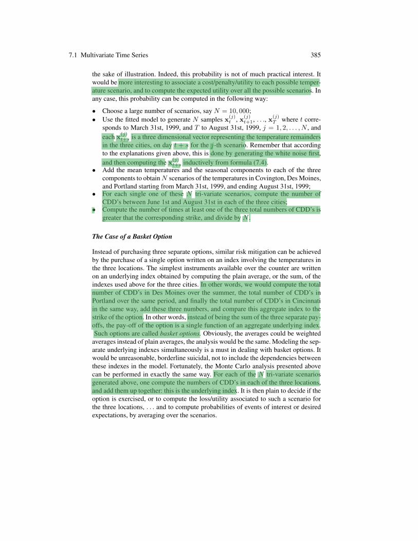
For the sake of illustration, we revisit the example of energy companies before andafter the crisis that followed Enron’s collapse. We already discussed in Subsection4.5.4, the case of American Electric Power (AEP). We now consider the weeklyexcess returns of another major electric utility, DUKE Electric Power, over the pe-riod starting 01/01/1995, and ending 12/10/2010. Our analysis of a time-dependentCAPM will shed some light on the effects of the energy crisis, and clearly exhibitfacts which are impossible to uncover in the classical time-independent setup. Thedata for AEP weekly excess returns are included in the library Rsafd and the readeris asked to perform this ”time-varying beta” analysis in Problem

Figure 7.4 shows the result of the non-anticipative estimation of the time varyingbetas by the Kalman filter. It shows that after a couple of years, the filter estimate ofbeta starts hovering below the level one, consistent with the fact that the stock was notconsidered risky before 2002. But despite the fact that DUKE was one of the very fewenergy companies to weather the crisis with little damage, its beta became greaterthan one in 2002 implying (according to the commonly admitted interpretation of thesize of the beta) that this stock became risky at that time. This phenomenon is presentfor all the companies that were affected by the energy crisis. This is illustrated forexample in Problem 7.13. For the sake of completeness, we give and comment theR code used to produce the results reproduced in Figure 7.4. We first set up theparameters of the state space model with partial observations as explained above.

GG <- seriesData(MARKET.wer.ts)NG <- length(GG)SIGMAV <- .0001; SIGMAW <- .0001YY <- seriesData(DUKE.wer.ts)NY <- length(YY)FF <- matrix(1,ncol=1,byrow=T)SigV <- matrix(SIGMAV,ncol=1)SigW <- matrix(SIGMAW,ncol=1)


0.40.6

0.81.0

1.21.4

2000 2005 2010

Time Series Plot of DUKE_BETA.ts

Fig. 7.4. Non-anticipative estimates of the DUKE time varying betas given by Kalman filteringover the period starting 01/01/1995 and ending 12/10/2010.

The computations of the one-step-ahead predictions are stored in a matrix Xhat asfollows:

Xhat <- matrix(rep(0,N),ncol=1)Xhat[1] <- .4Omega <- matrix(rep(0,N),ncol=1)Omega[1] <- .035for (n in 1:(N-1))

KALMAN <- kalman(FF=FF, SigV=SigV, GG[n], SigW=SigW,Xhat=Xhat[n], Omega=Omega[n], Y=YY[n])

Xhat[n+1] <- KALMAN$xpredOmega[n+1] <- KALMAN$error

Then the (simultaneous) values of the filter estimate of the unobserved ”beta” arecomputed, put in a timeSeries object and plotted.

DELTAn <- GG*Omega*GG + SIGMAWXhatnn <- Xhat + Omega*GG*(YY-GG*Xhat)/DELTAnOmegann <- Omega -Omega*GG*GG*Omega/DELTAnDUKE_BETA.ts <- timeSeries(positions=

seriesPositions(DUKE.wer.ts),data=Xhat)plot.timeSeries(DUKE_BETA.ts)

7.6 State Space Representation of Time Series 407

7.6 STATE SPACE REPRESENTATION OF TIME SERIES

As we already noticed, we are only considering state-space models whose dynamicsare given by a multivariate AR(1) series. Since some of the components of the statevector may remain unobserved, we can always add new components to the state vec-tor without changing the observations. This feature of the partially observed systemsmakes it possible to rewrite the equation defining an AR(p) model as an AR(1)-likeequation, simply by adding the components Xt−1, . . ., Xt−p to the value of a (newand extended) state at time t. Adding the past values to the current value of the stateenlarges the dimension, and this did not make sense when we were assuming thatthe entire state vector was observed. However, now that the observations are not nec-essarily complete, this transformation makes sense. This section takes advantage ofthis remark, but not without creating new problems. Indeed, a given set of observa-tions vectors may correspond to many state space vectors, and consequently, as inthe case of the factor models, we should be prepared to face a lack of uniqueness inthe representation of a given stochastic system as a state space system.

7.6.1 The Case of AR Series

Let us first consider the simple example of an AR(1) model. Let us assume for ex-ample that X ∼ AR(1), and more precisely that:

Xt = .5Xt−1 +Wt.

Switching to the index n, one can write:Xn+1 = .5Xn +Wn+1

Yn = Xn

This means that an AR(1) model is equivalent to a state space system describedby the one dimensional (i.e. dX = 1) state vector Xn = Xn, its dynamics beinggiven by the first of the equations above, the second equation giving the observationequation with Yn = Xn. Notice that the observations are perfect since there is nonoise term in the observation equation.

Since this example is too simple to be indicative of what is really going on, weconsider the case of an AR(2) model. Let us assume for example that:

Xt = .5Xt−1 + .2Xt−2 +Wt (7.29)

for some white noise Wt. Switching once more to the notation n for the timestamp, we rewrite this definition in the form:[

Xn+1

Xn

]=

[.5 .21 0

] [Xn

Xn−1

]+

[Wn+1

0

](7.30)


Indeed, if we look at this equality between two vectors, the equality of the first com-ponent of the left hand side with the first component of the right hand side givesback the definition (7.29) of Xn, while the equality between the second componentsis merely a consistency relation giving no extra information. Now, if for each timeindex n we define the two-dimensional (i.e. dX = 2) random vector Xn by:

Xn =

[Xn

Xn−1

](7.31)

the deterministic matrix F and the random vector Vn by:

F =

[.5 .21 0

]and Vn =

[Wn

0

],

then equation (7.30) becomes:

Xn+1 = FXn +Vn+1

which can be viewed as the equation giving the dynamics of the state X. Usingperfect observation, i.e. setting Yn = Xn, which corresponds to G = [1, 0] andWn ≡ 0, we see that we can represent our AR(2) series as a state-space model withperfect observation. We now show how this procedure can be generalized to all theAR models.

Let us now assume that Xnn is a mean-zero time series of the most generalAR(p) type given by the standard auto-regressive formula:

Xn = φ1Xn−1 + · · ·+ φpXn−p +Wn (7.32)

for some set of coefficients φ1, . . ., φp, and a white noise Wnn of unknown vari-ance. For each time stamp n we define the p-dimensional column vector Xn by:

Xn = [Xn, Xn−1, . . . , Xn−p+1]t.

There is no special reason to define Xn from its transpose, we are merely tryingto save space and make typesetting easier! Using this state vector, we see that wecan derive an observation equation of the desired form by setting Yn = Xn, G =[1, 0, . . . , 0], and Wn ≡ 0. This is again a case of perfect observation. Finally wewrite the dynamics of the state vector X in the form of definition (7.32). Adding theconsistency relations for the remaining components, this equation can be written inthe form:

Xn+1 =

Xn+1

Xn

...Xn+2−p

=

φ1 φ2 · · · φp−1 φp1 0 · · · 0 0...

......

......

0 0 · · · 1 0

Xn

Xn−1...

Xn+1−p

+

Wn+1

0...0

which can be viewed as the state equation giving the dynamics of the state vectorXn if we define the state matrix F and the state white noise Vn by:

7.6 State Space Representation of Time Series 409

F =

φ1 φ2 · · · φp−1 φp1 0 · · · 0 0...

......

......

0 0 · · · 1 0

and Vn =

Wn

0...0

.

7.6.2 The General Case of ARMA Series

We now assume that the time series Xnn satisfies:

Xn − φ1Xn−1 − · · · − φpXn−p =Wn + θ1Wn−1 + · · ·+ θqWn−q

for some white noise Wnn with unknown variance. Adding zero coefficient termsif necessary, we can assume without any loss of generality that p = q + 1. Usingthe notation introduced in the previous chapter this can be written in a condensedmanner in the form φ(B)X = Θ(B)W . LetU be an AR(p) time series with the samecoefficients as the AR - part of X , i.e. satisfying φ(B)U = W . If for example themoving average representation exists (but we shall not really need this assumptionhere) we saw that:

φ(B)U =W is equivalent to U =1

φ(B)W (7.33)

and consequently:

X =θ(B)

φ(B)W = θ(B)

1

φ(B)W = θ(B)U

which implies that:

Xn = Un + θ1Un−1 + · · ·+ θqUn−q

= [1, θ1, . . . , θq]

UnUn−1

...Un−q

which can be viewed as an observation equation if we set:

Yn = Xn, G = [1, θ1, . . . , θq], and Wn ≡ 0

and if we define the state vector Xn as the column vector with p = q+1 row entriesUn, Un−1, . . ., Un−p+1. So we have dY = 1 and dX = p = q + 1. Now that wehave the observation equation, we derive the state equation. Because of its definition(7.33), the time series U is an AR(p) series and φ(B)U =W can be rewritten in thestandard form:

Un − φ1Un−1 − · · · − φpUn−p =Wn


which is exactly the form we used in the previous subsection to rewrite the ARseries in a state-space form. So using the same procedure (recall that we arranged forp = q + 1)

Xn+1 =

Un+1

Un...

Un+2−p

=

φ1 φ2 · · · φp1 0 · · · 0...

......

0 0 · · · 1

UnUn−1

...Un+1−p

+

Wn+1

0...0

which can be viewed as the desired state equation giving the dynamics of the statevector Xn, if we define the matrix F as the p × p matrix appearing in the aboveequation, and if we define the noise vector Vn+1 as the p-dimensional column vectorwith components Wn+1, 0,. . ., 0.

Remarks1. As we already pointed out, the above representation is not unique.We gave an

algorithmic procedure which works in all cases, but one should keep in mind thatthere are many ways to define a state vector and its dynamics, while keeping thesame observations.

2. The above procedure can be implemented (modulo minor technical changesto accommodate the dimensions) in the case of multivariate time series, providing astate space representation of multivariate ARMA series.

7.6.3 Fitting ARMA Models by Maximum Likelihood

When explaining the limitations of R in fitting ARIMA models, we said that thestandard way to fit an MA(q) was to use the maximum likelihood method, but that thecomputation of the likelihood function was difficult, and that the only practical wayto do so was to use a recursive computation reminiscent of the filtering paradigm.Moreover, we also said at that time, that we suspected that this was the main reasonwhy fitting MA models was not implemented in R in the multivariate case. Now thatwe have seen the recursive Kalman filters, and that we know how to rewrite ARMAmodels in a state space form, it is time to revisit this fitting issue and shed some lighton the matter.

The only reason for not implementing the maximum likelihood estimation of anARMA model is the lack of filtering tools.

Indeed, given the order of an ARMA model, one can

• Use the algorithmic procedure presented in the previous subsection to rewrite themodel as a state space model;

• Follow the step outlined in Subsection 7.4.5 to compute the likelihood of any setof observations;

• Run our favorite optimization program to solve for the maximum of this likeli-hood function.

7.7 Example: Prediction of Quarterly Earnings 411

7.7 EXAMPLE: PREDICTION OF QUARTERLY EARNINGS

This section is devoted to a detailed discussion of a specific application of the re-cursive filters to the analysis of a financial problem. We show how to use the statespace representations and the recursive filtering equations to analyze a scalar timeseries which appears naturally as the sum of trend, seasonal and irregular compo-nents. Contrary to the strategy adopted in the case of temperature data, we do notassume that the trend and seasonal components are deterministic, and we do not startby removing them to reduce the problem to the analysis of a stationary time series.Instead, we include the trend and seasonal components in a structural model whichwe represent as a partially observed state-space model, which we predict using therecursive filtering equations.

We choose to illustrate this approach with the example of the prediction of thequarterly earnings of a public company. Figure 7.5 gives the plot of the time series of

0.10.2

0.30.4

1985 1990 1995 2000

Time Series Plot of GEqeps.ts

Fig. 7.5. Quarterly earnings per share of General Electric from March 31, 1983 to June 30,2002.

the quarterly earnings of General Electric starting March 31, 1983 and ending June30, 2002. Earnings per share used to be published yearly in 1982 and before. Thisseries is obviously non-stationary. In particular, it shows a significant upward trendand a seasonal component that cycles every four quarters, or once per year. Moreover,the scale of this seasonal component seems to fluctuate erratically, possibly gettinglarger over time. Since square root and logarithmic transformations do not seem toresolve the non-stationarity problem, we express the series directly as the sum of atrend component, a seasonal component and a white noise:


Yn = Tn + Sn + εn (7.34)

where the series Tnn models the trend, Snn models the seasonal component,and εnn is a white noise. Because the trend could be suspected to be exponential,we choose to model the trend as a time series satisfying an evolution equation of theform:

Tn+1 = φTn + ε(T )n+1 (7.35)

where ε(T )n n is a white noise independent of εnn, and where the real coefficient

φ is chosen to satisfy φ > 1. The evolution equation of Tn is the equation of anAR(1), but the assumption we make on the coefficient, namely φ > 1, guaranteesthat this AR series is not stationary. Instead of assuming that the seasonal componentis a deterministic periodic function of period 4, we assume that it is a series satisfyinga dynamical equation of the form:

Sn+1 = −Sn − Sn−1 − Sn−2 + ε(S)n+1 (7.36)

where ε(S)n n is a white noise independent of the two previous ones. The idea be-hind this choice is that at least in expectation, S should sum up to zero over a com-plete period of four quarters. All these requirements can be encapsulated inside apartially observed state-space model in the following way. First we define the statevector:

Xn = [Tn, Sn, Sn−1, Sn−2]t

so that dX = 4, and together with the obvious consistency conditions, equations(7.35) and (7.36) can be used to give the dynamics of the state via the equation:

Xn+1 =

Tn+1

Sn+1

SnSn−1

=

φ 0 0 00 −1 −1 −10 1 0 00 0 1 0

TnSnSn−1Sn−2

+

ε(T )n+1

ε(S)n+1

00

which can be viewed as the state equation giving the dynamics of the state vectorXn, if we define the matrix F as the 4 × 4 matrix appearing in the above equation,and if we define the noise vector Vn+1 as the 4-dimensional column vector withcomponents ε(T )

n+1, ε(S)n+1,0,0. Formula (7.34) used to define the model can now beused to give the observation equation for the one-dimensional observation vectorYn = yn:

Yn = [1, 1, 0, 0]

TnSnSn−1Sn−2

+ εn

which is of the desired form if we set G = [1, 1, 0, 0] and Wn = εn. The parametersof the model are the standard deviations σ, σ(T ) and σ(S) of the noise componentsintroduced above, as well as the parameter φ. The data is not very noisy, the chal-lenge lies in the fact that the time series is short for the filter to settle down and

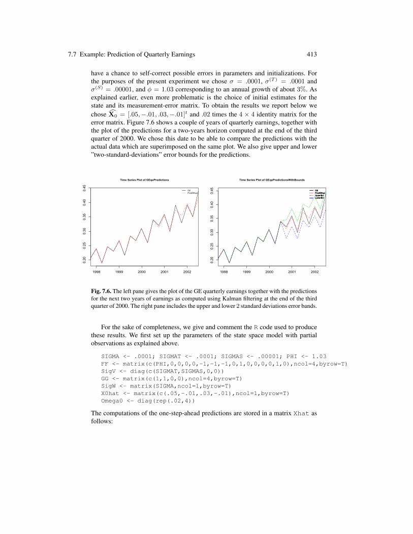
7.7 Example: Prediction of Quarterly Earnings 413

have a chance to self-correct possible errors in parameters and initializations. Forthe purposes of the present experiment we chose σ = .0001, σ(T ) = .0001 andσ(S) = .00001, and φ = 1.03 corresponding to an annual growth of about 3%. Asexplained earlier, even more problematic is the choice of initial estimates for thestate and its measurement-error matrix. To obtain the results we report below wechose X0 = [.05,−.01, .03,−.01]t and .02 times the 4 × 4 identity matrix for theerror matrix. Figure 7.6 shows a couple of years of quarterly earnings, together withthe plot of the predictions for a two-years horizon computed at the end of the thirdquarter of 2000. We chose this date to be able to compare the predictions with theactual data which are superimposed on the same plot. We also give upper and lower”two-standard-deviations” error bounds for the predictions.

0.20

0.25

0.30

0.35

0.40

0.45

1998 1999 2000 2001 2002

Time Series Plot of GEqePredictions

GEPredGEqe

0.20

0.25

0.30

0.35

0.40

0.45

1998 1999 2000 2001 2002

Time Series Plot of GEqePredictionsWithBounds

GEPredGEqeUpperBdLowerBd



Fig. 7.6. The left pane gives the plot of the GE quarterly earnings together with the predictionsfor the next two years of earnings as computed using Kalman filtering at the end of the thirdquarter of 2000. The right pane includes the upper and lower 2 standard deviations error bands.

For the sake of completeness, we give and comment the R code used to producethese results. We first set up the parameters of the state space model with partialobservations as explained above.

SIGMA <- .0001; SIGMAT <- .0001; SIGMAS <- .00001; PHI <- 1.03FF <- matrix(c(PHI,0,0,0,0,-1,-1,-1,0,1,0,0,0,0,1,0),ncol=4,byrow=T)SigV <- diag(c(SIGMAT,SIGMAS,0,0))GG <- matrix(c(1,1,0,0),ncol=4,byrow=T)SigW <- matrix(SIGMA,ncol=1,byrow=T)X0hat <- matrix(c(.05,-.01,.03,-.01),ncol=1,byrow=T)Omega0 <- diag(rep(.02,4))

The computations of the one-step-ahead predictions are stored in a matrix Xhat asfollows:


Xhat <- matrix(rep(0,284),ncol=71,byrow=T)Xhat[,1] <- X0hatOmega <- Omega0for (n in 1:70)

KALMAN <- kalman(FF=FF, SigV=SigV, GG=GG, SigW=SigW,Xhat=Xhat[,n], Omega=Omega, Y=seriesData(GEqeps.ts)[n])

Xhat[,n+1] <- KALMAN$xpredOmega <- KALMAN$error

Finally, the actual predictions of the observations, together with the upper andlower bounds, are computed and stored in the timeSeries objects GEpred.ts,GEpredUB.ts, and GEpredLB.ts respectively.

XPRED <- matrix(rep(0,36),ncol=9,byrow=T)YPRED <- rep(0,8)YVAR <- rep(0,8)XPRED[,1] <- Xhat[,71]MAT <- GGfor (I in 1:8)

YPRED[I] <- GG %*% XPRED[,I]XPRED[,I+1] <- FF %*% XPRED[,I]YVAR[I] <- MAT %*% Omega %*% t(MAT)MAT <- MAT %*% FF

The plots of Figure 7.6 were produced with the following commands.

GEpred.ts <- timeSeries(pos=seriesPositions(GEqeps.ts),data=c(seriesData(GEqeps.ts)[1:70],YPRED),units="PredGEqe")

GEpredUB.ts <- timeSeries(pos=seriesPositions(GEqeps.ts),data=c(seriesData(GEqeps.ts)[1:70],YPRED+2*sqrt(YVAR)),units="UpperBd")

GEpredLB.ts <- timeSeries(pos=seriesPositions(GEqeps.ts),data=c(seriesData(GEqeps.ts)[1:70],YPRED-2*sqrt(YVAR)),units="LowerBd")

GEqePredictions <- merge(GEqeps.ts[59:78],GEpred.ts[59:78])plot.timeSeries(GEqePredictions)

GEqePredictions <- merge(GEqePredictions,GEpredUB.ts[59:78])GEqePredictionsWithBounds <- merge(GEqePredictions,GEpredLB.ts[59:78])plot.timeSeries(GEqePredictionsWithBounds)

PROBLEMS

©E©S Problem 7.1 The purpose of this problem is to examine the various ways the componentsof a multivariate time series can be dependent. We consider the following AR(1) model for abivariate time series Xtt=0,1,···:

Problems 415

Xt = AXt−1 + Wt, t = 1, 2, · · ·

where:

X =

[X

(1)t

X(2)t

], and A =

[.2 00 .4

],

and where Wtt is a bivariate Gaussian white noise with covariance matrix

Σ =

[.2 00 1

].

1. Give a condition on the initial random variables X(1)0 and X(2)

0 which guarantees thatall the random variables X(1)

t and X(2)s are independent for the various values of t and s.

Explain why. From now on we assume that this condition is satisfied.2. Explain how one can change some of the entries of the matrix A to make sure that the timeseries X(1)

t t and X(2)t t are dependent.

3. Setting back the entries of the matrixA to their original values, explain how one can changesome of the entries of the matrix Σ to make sure that the time series X(1)

t t and X(2)t t

are dependent.4. Can you identify the differences in the statistical properties resulting from these two proce-dures? You can use simulations if you cannot quantify these differences theoretically.

The goal of problems 7.2, 7.3 and 7.5 is to quantify various risk exposures associatedwith temperature basket options similar to the one analyzed in the text. The data needed forthese problems are contained in the timeSeries objects TEMPS1.ts and TEMPS2.tsincluded in the library Rsafd.

©E Problem 7.2 This problem uses the data contained in the timeSeries object TEMPS1.ts.For each day of the period P starting from 09/06/1948 (the first row) and ending 11/08/2001(the last row) it gives the daily average temperatures recorded at the meteorological stations ofthe international airports of Reno (first column), Las Vegas (second column) and Sacramento(third column). We consider two time periods.

• Period P is the period of the measurements reported in TEMPS1.ts• Period P ′ is the period of the option for which one needs to predict the number of heating

degree days. It starts on 12/1/2001 and ends 2/28/2002 inclusive.

We consider a basket option written on the average number of heating degree days over thesethree cities. On each given day one computes the average of the three following numbers: thenumber of heating degree days in Reno, the number of heating degree days in Las Vegas, andthe number of heating degree days in Sacramento. One then computes the sum of these dailyaverages over the period P ′, and one compares this sum to the strike of the option, using thesame rules as usual to compute the pay-off of the option. The purpose of this problem is toperform a simple regression analysis of such a basket option.0. For each year in the period from 1961 to 2000 inclusive, compute the yearly index of theoption, compute the average of these yearly indexes over the last 15 years of this period, andcall this average K.

From now on we consider a European call option at the money (i.e. with strike K com-puted above), with tick α equal to US$ 5,000 per degree day, and cap US$ 1,000,000, writtenon the cumulative average number of HDD’s in Reno, Las Vegas and Sacramento from De-cember 1, 2001 to February 28, 2002.

AZhao

Highlight

AZhao

Highlight

AZhao

Pencil

AZhao

Pencil


1. Use the linear regression approach introduced in Problem 6.16 to give an estimate of theunderlying index on which the basket option is written, i.e. of the average of the three numbersof HDD in the cities of Reno, Las Vegas and Sacramento over the period P ′, and give a 95%confidence interval for this prediction.2. Answer questions 2. and 3. of Problem 6.16 in the present situation.

©E Problem 7.3 Follow the steps of the joint analysis of the daily average temperatures at the DesMoines, Portland and Cincinnati given in Subsection 7.1.4 of the text, and use the data of theperiod P to fit a trivariate model to the daily average temperatures in Reno, Las Vegas andSacramento of the timeSeries object TEMPS1.ts. Use this fitted model and follow theprescriptions given in the text to derive an estimate of the value of the average of the threenumbers of HDD’s in the cities of Reno, Las Vegas and Sacramento over the period P ′, andto provide new answers to the questions of Problem 7.2 above.

©E Problem 7.4 The goal of this problem is to quantify the risks and rewards of some hybridderivatives written on temperature and energy commodities. The data are contained in thedata set TempGasNorthGate.ts, a bivariate timeSeries object whose first columngives the daily average temperature at NorthGate and the second column, the price of themonth ahead contract of natural gas for delivery at NorthGate.1. We first study the temperature data.

1.1. For each year j ∈ J = 1980, 1981, · · · , 2007, 2008 compute the yearly indexHDD[j] as the sum of the daily HDD’s over the period P comprising the months of Januaryand February of year j. Compute the average of these yearly indexes over the last 15 years ofthis period, and call this average KT .

1.2. Decompose the time series of daily average temperatures at NorthGate into a trend, aseasonal component, and a remainder which you call TREND, SEA, and REM respectively. Fitan auto-regressive model to REM and report the order and the estimates of the coefficients. Fita distribution to the residuals.

1.3. Use N = 1000 Monte Carlo simulations to compute an approximation of the prob-ability that the cumulative number of HDDs over the period P in 2009 will exceed KT , inother words, provide a Monte Carlo approximation of the probability

PHDD[2009] > KT.

2. We now analyze the natural gas prices at NorthGate. For the sake of convenience we letG[t] denote the price of the contract of natural gas on day t. The number KG will denote theaverage daily natural gas price over the last 5 years. Compute its value.

2.1. Compute and plot the time series LR of daily log-returns of the natural gas contract.Fit an auto-regressive model to LR and report the order, the estimates of the coefficients, andfit a distribution to the residuals.

2.2. Use N = 1000 Monte Carlo simulations to compute an approximation of the expec-tation

E∑t∈P

(G[t]−KG)+,

namely the expected cumulative amount by which the daily price overshoots the level KGover the period P in 2009. The sum appearing in the expectation will be called the overshootand we will denote it by OV ER.

AZhao

Pencil

Problems 417

3. Assuming that we need to buy gas every day of the period P in 2009, and that we do notwant to pay more than KG on any given day, we enter before December 31, 2008 into acontract which guarantees the pay-off

PAY OFF [2009] = 1HDD[2009]>KT∑t∈P

(G[t]−KG)+

at the end of the period P . In other words, assuming that we purchase one unit of gas every-day, this hybrid derivative guarantees that, if at the end of the month of February 2009, thecumulative number of HDDs over the period P exceeds the strike KT , then we are paid theovershoot for all the days we had to buy gas at a price higher than the strike KG.Use N = 1000 Monte Carlo simulations and compute approximations of the probabiliy thatthe pay-off (at the end of the period P in 2009) is non zero, and the expected pay-off.4. We now assume that we will need to buy (one unit of) gas every day of period P in 2009and every day of period P in 2010 as well, and we buy an option which guarantees the pay-off PAY OFF [2009] if we decide to exercise our option at the end of February 2009, orthe pay-off PAY OFF [2010] if we decide not to exercise our option at the end of February2009. Clearly, the decision to exercise or not to exercise the option at the end of February2009 should be made at that time, i.e. on the basis of information available at that time. Also,PAY OFF [2010] is defined similarly to PAY OFF [2009], using the HDDsand the dailyprices during the period P of 2010.Generate N = 1000 Monte Carlo samples of the temperature nd the price of naturalgas at NorthGate over the period ranging from January 1, 2009 to the last day of Febru-ary 2010. For each scenario n = 1, 2, · · · , 1000, compute HDD[2009, n] the number ofHDDs over the period P in 2009, HDD[2010, n] the number of HDDs over the periodP in 2010, OV ER[2009, n] the overshoot of the gas price over the period P in 2009,and OV ER[2010, n] the overshoot over the period P in 2010, Next, compute the payoffsPAY OFF [2009, n] and PAY OFF [2010, n] using the defining formula given above.

©E Problem 7.5 This problem provides another numerical illustration of the points addressedin Problems 6.16, 7.2 and 7.3. The data needed for this problem are contained in thetimeSeries object TEMPS2.ts giving the daily average temperatures, starting from1/1/1972 (the first row) ending 12/31/2001 (the last row) at the meteorological stations ofNewark, La Guardia and Philadelphia. The data have been cleaned in the sense that all theFebruary 29th’s of the leap years of this period have been removed. For the purpose of thequestions below, we shall use two time periods.

• Period P is the period of the time stamps of the timeSeries object.• Period P ′ is the period for which you will need to predict the number of cooling degree

days (CDD’s for short). It starts on 5/1/2002 and ends 9/30/2002 inclusive.

0. For the location Newark, and for each year in the period P , compute the yearly CDD index,i.e. the total number of CDD’s between May 1, and September 30 of that year (these two daysbeing included). Bundle these yearly aggregates into a vector which we shall call INDEX.1. Using only the numerical values contained in the vector INDEX

a) Compute a prediction for the value of the yearly cumulative number of CDD’s in Newarkfor the period P ′.

b) Give a 95% confidence interval for this predictionc) Let us assume that on January 1, 2002, you buy a call option on the number of CDD’s

in Newark over the period P ′, with strike K being equal to the average of the yearly numbers


Newark La Guardia PhiladelphiaNumber of CDD’s during P ′ 1325 1355 1463.5

of CDD’s over the last 15 years, nominal pay-off rate (also called the tick) $ 5000, and cap $1000000 for a premium of $ 400000. Use the linear model so fitted to give an estimate of theprobability that you will loose money on this deal?

d) Compute your profit/loss, should the prediction you computed in part a) be perfect inthe sense that it is equal to the actual number of CDD’s which accumulated over the periodP ′.2. Use the daily data in the period P to fit a model to the average daily temperature in Newark,and use this estimated model to propose new answers to the questions a) through d) above.Compare the results for each of these questions.3. Give an estimate and a 95% confidence interval for the average of the three numbers ofCDD’s in the cities of Newark, La Guardia and Philadelphia over the period P ′,4. Let us assume that on January 1, 2002, you want to buy from me a ”basket” call option atthe money, on the average of the numbers of CDD’s in Newark, La Guardia and Philadelphiaover the period P ′, with the same tick and the same cap as above. Say how much you wouldbe willing to buy this option for, and explain why.FYI: Even though you should not use these numbers in the solutions of the questions above,you should know the actual numbers of CDD’s over the period P ′ in these three cities. Theyare reproduced in Table 7.5.

©E Problem 7.6 The data needed for this problem are contained in the timeSeries objectTEMPS3.ts. The latter gives the daily temperatures, starting from 1/1/1981 (the first row)ending 1/11/2010 (the last row) at the meteorological stations of Saint Etienne and Aix enProvence in France. The data have been cleaned in the sense that all the February 29th’s ofthe leap years of this period have been removed. For the purpose of the questions below, weshall use two time periods.

• Period P is the period of the time stamps of the timeSeries object.• Period P ′ is the period for which you will need to predict the temperature in these cities.

It starts on 1/15/2010 and ends 1/31/2010 inclusive.

0. For each of the two locations, and for each year in the period P , compute the averagetemperature over the period Jan. 15 – 31, and the number of HDDs over the same period.Bundle these yearly statistics into two separate matrices each with two columns and as manyrows as years in the period P: a matrix TEMP for the average temperature, and a matrix HDDfor the number of HDDs.1. The questions of this first part rely on linear regression.

a) Using only the numerical values contained in TEMP , fit a linear model to the yearlyaverage temperature in Saint Etienne over the period Jan. 15 – 31, compute a prediction forthe value of this variable in 2010, and give a 95% prediction interval for this prediction.

b) Using only the numerical values contained in TEMP , fit a linear model to the yearlyaverage temperature in Aix en Provence over the period Jan. 15 – 31, compute a predictionfor the value of this variable in 2010, and give a 95% prediction interval for this prediction.

c) Using only the numerical values contained in HDD , fit a linear model to the yearlynumber of HDDs in Saint Etienne over the period Jan. 15 – 31, compute a prediction for thevalue of this variable in 2010, and give a 95% prediction interval for this prediction.

Problems 419

d) Using only the numerical values contained in HDD , fit a linear model to the yearlynumber of HDDs in Aix en Provence over the period Jan. 15 – 31, compute a prediction forthe value of this variable in 2010, and give a 95% prediction interval for this prediction.2. Use the daily data originally given in TEMPS3.lts to fit a model to the daily temperaturein both locations, and use your fitted model to propose new answers to the questions a) throughd) above. Compare the results for each of these questions.

We now consider a call option option (without cap) on the sum over the period Jan. 15– 31, 2010, of the numbers of HDDs in the two cities, with strike given by the mean of thisquantity over the last 15 years, and tick 1000 EUR per HDD.3. Using ALL the models constructed above which can provide sensible answers, give esti-mates of

• The probability that the option is exercised;• The expected pay-off of the option at maturity.

4. Compute for each day of the period P, the sum of the temperature in Saint Etienne and inAix en Provence, call Y the numeric vector so obtained, and assume that instead of actuallyobserving the temperatures in the two cities separately, one has access to the value of Y only,and up to a Gaussian noise with variance 2.6 independent each day. Assuming that the modelyou fitted in question 2 above is correct, how would you go about answering the two questionsgiven in the bullet points of question 3 if the option was written on the average temperature inAix en Provence instead? Assume that the strike is given by the mean of this quantity over thelast 15 years and that the tick is 1000 EUR per HDD.

©S Problem 7.7 The purpose of this problem is to illustrate by simulation the cointegration prop-erties stated in the example given at the beginning of Subsection 7.1.61. Construct a sample Wnn=1,...,N of sizeN = 1024 from the normal distributionN(0, 1),construct the random walk Sn = S0+W1+. . .+Wn starting from S0 = 0, and construct twoindependent white noise sequences ε(1)n n=1,...,N and ε(2)n n=1,...,N from the distributionN(0, .16) which are independent of Wnn=1,...,N . Give on the same figure the plots of thegraphs of the time series X(1)

n n=1,...,N and X(2)n n=1,...,N defined by:

X(1)n = Sn + ε(1)n and X(2)

n = Sn + ε(2)n .

2. Give the plot of the linear combination of X(1)n n=1,...,N and X(2)

n n=1,...,N given bythe cointegration vector identified in the text, compare to the previous plot and explain why itconfirms cointegration.3. Construct two independent samples W (1)

n n=1,...,N and W (2)n n=1,...,N of size N =

1024 from the normal distribution N(0, 1), construct the random walks S(1)n = S

(1)0 +

W(1)1 + · · · + W

(1)n and S

(2)n = S

(2)0 + W

(2)1 + · · · + W

(2)n starting from S

(1)0 = 0

and S(2)0 = 0 respectively, and construct as before two independent white noise sequences

ε(1)n n=1,...,N and ε(2)n n=1,...,N from the distribution N(0, .16) which are independent ofW (1)

n n=1,...,N and W (2)n n=1,...,N . Give on the same figure the plots of the graphs of the

time series X(1)n n=1,...,N and X(2)

n n=1,...,N defined by:

X(1)n = S(1)

n + ε(1)n and X(2)n = S(2)

n + ε(2)n .

4. Give the plot of the same linear combination of X(1)n n=1,...,N and X(2)

n n=1,...,N asbefore, compare to the plot obtained in part 2, and explain why there is no cointegration thistime.


5. Give the scatterplot of X(2)n against X(1)

n , add the least squares regression line, test ifthe regression is significant, and give a time series plot of the residuals as well as their acf.Comment.

©S Problem 7.8 We consider the state-space model given by:Xt+1 = FXt + VtYt = GXt +Wt

where the covariance matrices of the white noises Vtt and Wtt are the identity matricesand where the other parameters are given by:

F =

.2 −.1 31 0 00 1 0

, and G =

[1 1 00 1 1

].

We assume that the values of the one step ahead estimates Xt0 of the state vector, and Ωt0 ofits covariance matrix are given by:

Xt0 =

1.2.3.45

, and Ωt0 =

1.25 1 11 1.25 11 1 1

.We also assume that the next 5 values of the observation vector Y are given by:

Yt0 =

[−.11

], Yt0+1 =

[.3

.9

], Yt0+2 =

[.47

−.8

], Yt0+3 =

[.85

−1.0

], Yt0+4 =

[.32

.9

].

For each time t = t0 + 1, t = t0 + 2, t = t0 + 3, t = t0 + 4 and t = t0 + 5, use Kalmanfiltering to compute the one step ahead estimates Xt, its prediction quadratic error Ωt, andof the next observation vector Yt|t−1, and its prediction quadratic error ∆(1)

t−1.

©S Problem 7.9 The goal of this problem is to write S-functions to simulate and visualize the timeevolution of the state and the observation of a linear state-space system of the form:

Xt+1 = FXt + Vt

Yt = GXt + Wt(7.37)

where both the state vector Xt and the observation vector Yt are of dimension 2, and whereVtt and Wtt are independent Gaussian white noises with variance/covariance matricesΣV andΣW respectively. As usual we assume that Vt and Wt are independent of Xt, Xt−1,Xt−2, . . .. We shall also visualize the performance of the forecasts derived from the Kalmanfilter theory.1. Write an S-function, say ksim, with parameters F, G, SigV, SigW, X0, Omega0, N andSEED which:

• initializes the seed of the random generator of R to SEED• uses the random number generation functions of R to create aN×2 array of type numeric

containing realizations of the N values Vt; t = 0, 1, . . . , N − 1 of the white noiseand a 2 × (N + 1) array of type numeric containing realizations of the N + 1 valuesXt; t = 0, 1, . . . , N of the state vector Xt of the linear system given by equation(7.37) starting with X0 = X0

Problems 421

• Create an (N + 1) × 2 array of type numeric containing realizations of the N + 1values Wt; t = 0, 1, . . . , N of the observation white noise and uses the values of thestate vector created above to produce an (N + 1) × 2 array of type numeric containingrealizations of theN + 1 values Yt; t = 0, 1, . . . , N of the observations Yt satisfyingthe observation equation

• assume that X0 is perfectly known at time t = 0 (this is obviously an unrealistic assump-tion but please bear with me, this is merely homework stuff) and compute for t = 1, . . . , Nthe value of Xt|t = EXt|Y≤t, Xt = EXt+1|Y≤t and Yt = EYt+1|Y≤t andreturn the list of the five Nx2 arrays of type numeric say $xt, $yt, $hxtt, $hxtand $hyt containing the values of Xt, Yt, Xt|t, Xt and Yt for t = 1, . . . , N

We use the notation Y≤t = Yt, Yt−1, . . . , Y0 for the set of all the observations prior totime t. Recall that the notation Et(X) was used for what is now denoted by Xt|t.2. Run the S command

> KTST <- ksim(F, G, SigV, SigW, X0, Omega0, N, SEED)

with:

F =

[.2 −.11 .3

], and G =

[1 10 1

],

SigV =

[.2 00 1

], SigW =

[1 00 .4

], X0 =

[1.2.45

]and Omega0 =

[1.25 00 1.25

],

and finally with N = 125 and SEED = 14.3. Write an S function, say kanim which, with the appropriate parameters taken from the listKTST obtained in the previous question, will produce the following three animations.

• plots on the same graphic window of the successive values of KTST$xt and KTST$hxtt• plots on the same graphic window of the successive values of KTST$xt and KTST$hxt• plots on the same graphic window of the successive values of KTST$yt and KTST$hyt

©T Problem 7.10 Find the state-space representation for the following time series models:1. (1− φ1B)Yt = (1− θ1B)εt2. Yt = φ1Yt−1 + εt − θ1εt−1 − θ2εt−2

where in both cases, εtt denotes a white noise.

©T Problem 7.11 Let Xtt be the AR(1) time series:

Xt = φXt−1 + Vt

and let Yt be the noisy observation:

Yt = Xt +Wt

where we assume that Vtt and Wtt are independent Gaussian white noises with vari-ances σ2

V and σ2W respectively. Give the best predictions (in the sense of the expected squared

error) for Xt+1, Yt+1 and their variances given the past observations Yt, Yt−1, . . . .

©T Problem 7.12 Derive a state space representation for the ARIMA(1,1,1) model:

(1− φB)(1−B)Xt = (1− θB)Wt

when Wtt is a N(0, σ2) white noise, and identify all the parameters of the model in termsof φ, θ, and σ2 . Recall that (1−B) merely stands for the operation of differentiation.


©E Problem 7.13 Use the data of the weekly excess returns of AEP contained in the timeSeriesobject AEP.wer.ts to produce the same results as those reported in Subsection 4.5.4 forDUKE, by following all the steps of the filtering analysis of the time varying extension of theCAPM theory described in the text. Compare the beta estimates so obtained to those given inthe text for DUKE. Use the timeSeries object MARKET.wer.ts for the weekly excessreturns of the market portfolio. These excess returns were computed from the weekly returnsof the S&P500 index.

©E Problem 7.14 The data needed for this problem are contained in the timeSeries objectsPEPqeps.ts and IBMqeps.ts giving the quarterly earnings per share of Pepsi Co. andIBM.1. Use the Pepsi data and reproduce the filtering analysis done in the text for the DUKE Energyquarterly earnings.2. The goal of this second question is to perform the same analysis for IBM.2.1. Fit a state space model and use it to predict the last two years of quarterly earnings usingonly the data up to the last quarter of 2000.2.2. Fit a state space model to the data of the quarterly earnings over the period startingwith the first quarter of 1996, and ending with the third quarter of 2000. Use this model andKalman filtering as above to predict the last two years of quarterly earnings using only thedata used to fit the model.2.3. Fit a model to the data up to the last quarter of 1990, and use it to predict the quarterlyearnings of the period 1991-1995 using only the data up to the last quarter of 1990.2.4. Comment on the performance of the prediction in each case.

NOTES & COMPLEMENTS

Despite serious technical complications, the linear theory of time series presented in the previ-ous chapter in the univariate case can be extended to multivariate time series models. A thor-ough account can be found in Hamilton’s exhaustive expose in his book [33]. Cointegrationis a concept of great theoretical significance, and it is now an integral part of most economet-ric theory textbooks. It was introduced in the seminal work [25] of Engle and Granger. Thisfundamental contribution was cited as the main reason to grant the 2003 Nobel prize to theseauthors. The interested reader can also consult Johansen’s book [41] for the general statisticaltheory of cointegrated time series. Cointegration appears in economic theories as a way toimply equilibrium relationships between economic time series. These equilibria are the resultof relaxation of the dynamics toward steady states and identifying them usually requires longspans of low frequency data, for some form of ergodicity to take effect. In financial appli-cations, cointegration appears as a way to identify arbitrage opportunities. See for exampleSection 8.6 entitled Threshold cointegration and arbitrage of Tsay’s book [74]. A completeexpose of cointegration theory would be beyond the scope of this book. Nevertheless, we men-tion that its importance is now recognized by the financial engineering community as well asthe econometric community, and new research programs have been started to understand andcontrol better pricing and risk management issues in the presence of cointegrated price series.Spread options in the energy markets, and basket options in the equity markets are two of themany examples of instruments naturally written on cointegrated price series. Our interest inthese financial products drove our attempt to introduce the concept of cointegration, even ifwe knew that we could not make justice to its importance. The recent textbooks of Chan [18],

7 multivariate time series, linear systems and...

Documents